Black Holes, Oscillating Instantons, and the Hawking-Moss transition

Abstract

Static oscillating bounces in Schwarzschild de Sitter spacetime are investigated. The oscillating bounce with many oscillations gives a super-thick bubble wall, for which the total vacuum energy increases while the mass of the black hole decreases due to the conservation of Arnowitt-Deser-Misner (ADM) mass. We show that the transition rate of such an “up-tunneling" consuming the seed black hole is higher than that of the Hawking-Moss transition. The correspondence of analyses in the static and global coordinates in the Euclidean de Sitter space is also investigated.

1 Introduction

Cosmological phase transitions involving supercooling and the formation of bubbles may have played an important role in the early universe. In the case of extreme supercooling, the phase transition involves a quantum transition of a scalar field through a potential barrier from a false vacuum state to a true vacuum state. The vacuum decay rate is conventionally described in terms of an instanton, or bounce solution, to the field equations in imaginary time coleman1977 ; callan1977 ; CDL . In an interesting recent twist, primordial black holes Gregory:2013hja ; Burda:2015isa ; Burda:2015yfa ; Burda:2016mou ; Mukaida:2017bgd ; Oshita:2019jan and horizonless compact objects Oshita:2018ptr ; Koga:2019mee have been shown to act as nucleation seeds for true vacuum bubbles, and significantly enhance the decay rate (see also early work Hiscock:1987hn ; Berezin:1987ea ; Berezin:1990qs ). There is however another type of tunnelling solution – the Hawking-Moss (HM) instanton Hawking:1981fz – that is relevant for relatively flat potentials, and the aim of this paper is to explore how seeded nucleation proceeds in this case.

We are interested in situations where gravitational effects on bubble nucleation are important. This was first investigated by Coleman and de Luccia (CDL) CDL , who looked at bounce solutions to the Einstein-scalar system with $O(4)$ symmetry. Shortly after their work, in the context of the inflationary universe, Hawking and Moss noticed that CDL bounce solutions did not exist for very flat potentials, and instead suggested an $O(5)$ symmetric bounce solution, the HM instanton, was the appropriate solution. The nucleation rate obtained this way has since been supported by quantum cosmology Hartle:1983ai and by stochastic methods Starobinsky:1986fx . The HM instanton is static, and consists of a solution purely at the top of the potential barrier. These features are shared by bounce solutions in thermal systems, and a modern interpretation of the HM instanton is that it represents a thermal fluctuation within a horizon volume at the temperature of de Sitter (dS) space Brown:2007sd .

The condition for the existence of CDL instantons can be given explicitly in terms of the scalar potential $V$ and its second derivative at the top of the potential barrier Hawking:1981fz ; Hackworth:2004xb ; Balek:2004sd ; Weinberg:2005af ; Kanno:2011vm ; Battarra:2013rba

$$\left|{d^{2}V\over d\phi^{2}}\right|>4\left({8\pi V\over 3M_{\rm Pl}^{2}}\right)$$ (1)

where $M_{\rm Pl}\equiv 1/\sqrt{G}$ is the Planck mass. This condition is relaxed when the fourth derivative $d^{4}V/d\phi^{4}$ is subdominant Demetrian:2005ag . Furthermore, close to this bound there are typically multiple solutions of an oscillatory type which oscillate back and forth between either side of the potential barrier Hackworth:2004xb ; Lavrelashvili:2006cv ; Lee:2012qv ; Lee:2014ula . Like the HM instanton, these may be regarded as thermal excitations, however, it has been suggested that the oscillatory solutions have more than one negative mode and because of this cannot represent true vacuum decay Lee:2014ula .

Seeded vacuum decay by a primordial black hole Burda:2015isa ; Burda:2015yfa ; Burda:2016mou is another case which has a close resemblance to thermally assisted quantum tunnelling, however this time at the Hawking black hole temperature. In fact, the tunnelling rate can be expressed thermodynamically using Boltzmann’s formula Gregory:2013hja ; Oshita:2016oqn ,

$$\Gamma=Ae^{\Delta{\cal S}},$$ (2)

where $A$ is the pre-factor and $\Delta{\cal S}$ is the change in black hole (BH) entropy due to the loss of mass during the tunnelling event. (The entropy can go down in a fluctuation, which is why this is an unlikely event). The BHs break some of the symmetry, so that the bounce solutions have $O(3)$ symmetry. However, the bounces that dominate the decay rate are also imaginary-time translation invariant, as we would expect from the thermal context. These bounces were investigated primarily in the context of Higgs decay in an asymptotically flat universe, however, here we examine the more general question of when seeded bounce solutions exist, and present new results on seeded HM tunnelling. We are therefore looking at the early universe in situations where the potential barrier is close to the limit in Eq. (1).

In this manuscript, we investigate oscillating bounces in the Schwarzschild de Sitter (SdS) background using static coordinates. The organization of this manuscript is as follows: Before embarking on the analysis in the static SdS background, in Sec. 2 we first investigate analytically the oscillating bounce solutions, both for a dS background as well as close to the Nariai limit Nariai:1 ; Nariai:2 , using the static SdS co-ordinates. This contrasts to the conventional analysis, such as in Hackworth:2004xb , that are performed in global dS coordinates. We carefully show that the analysis in both static and global dS patches lead to the same eigenvalue restrictions on $V^{\prime\prime}(\phi_{\rm top})/(M_{\rm Pl}^{2}V)$ (where a prime denotes the derivative with respect to $\phi$) for a probe solution, as well as the same functional form for the scalar perturbation. This is a highly nontrivial result, as the analytic continuation of the global and static patches does not coincide, and of course the coverage of the static patch in the Lorentzian section is not the full dS spacetime. Sec. 3 presents the oscillating bounce solutions in a general SdS background, obtained by solving the (non-linear) Einstein-scalar field equations with time-translation and spherical symmetry. Then we constrain the parameter region of the mass of a seed BH and $V^{\prime\prime}(\phi_{\rm top})/(M_{\rm Pl}^{2}V)$ in which the oscillating bounces exist. In Sec. 4 we discuss the HM bounce around a BH, that conserves the total energy inside the cosmological horizon, and compare its bounce configuration and Euclidean action with those of the oscillating bounce with many oscillations. Then we conclude that the higher-mode oscillating bounces may be regarded as the intermediate bounces between the fundamental bounce (no turning point for $\phi$) and the HM bounce around a BH. We conclude in the final section.

2 Oscillating Bounce in Static Patch: dS and Nariai Limits

The $O(4)$ symmetric oscillating bounce solutions were analysed close to the critical limit of (1) by Hackworth and Weinberg Hackworth:2004xb . The argument runs as follows: Any bounce solution interpolating between vacua must pass over the top of the potential, therefore, in the limit of a very thick wall we can regard the bounce as a perturbation of the solution that sits on the top of the potential ($\phi=\phi_{\rm top}$) and linearize the equations of motion around this exact dS solution. To leading order, we have the equation for the scalar field $\phi=\phi_{\rm top}+\delta\phi$:

$$\Box\delta\phi\approx V^{\prime\prime}(\phi_{\rm top})\delta\phi,$$ (3)

with the geometry corrected at order ${\cal O}(\delta\phi^{2})$. They analysed this scalar equation in the dS background, discovering that it yielded an eigenvalue equation for $\beta=3V^{\prime\prime}(\phi_{\rm top})/(8\pi GV_{\rm top})$, hence a lower bound on $\beta$ for the oscillating bounce solutions, where $V_{\rm top}\equiv V(\phi_{\rm top})$. This eigenvalue equation represents solutions for $\delta\phi$ that remain fully within the perturbative régime, however, does not mean there are no solutions for other values of $\beta$, only that these will enter the régime in which the nonlinear corrections to $V^{\prime\prime}(\phi)$ become important, as described below.

We will now present an analogous calculation for the seeded decay, however note that a BH in dS space, described by the SdS solution, is written in ‘static’ coordinates, i.e. there is no time-dependence in the metric. The analysis of Hackworth:2004xb however (and indeed the original CDL bounce) is performed in global – time dependent – dS coordinates. We must therefore first demonstrate that the unstable dS solution presents the same eigenvalue restrictions on $\beta$, although the eigenfunction solutions for $\delta\phi$ may be different in this patch, due to the different analytic continuation. We should emphasise that this is a highly nontrivial requirement, as the analytic continuation for the $O(4)$ instanton in the global patch is different to the analytic continuation for the static patch.

Lorentzian de Sitter spacetime can be represented as a hyperboloid embedding within a 5D Minkowski spacetime. For future discussion, we note the transformation between the static and global dS coordinates, denoted by $(t,r,\theta,\varphi)$ and $(T,y,\theta,\varphi)$, respectively, via the hyperboloid embedding:

$$\sin y\sinh(HT)= X^{0}=\sqrt{1-H^{2}r^{2}}\sinh(Ht),$$ (4)

$$\cos y= X^{1}=\sqrt{1-H^{2}r^{2}}\cosh(Ht),$$

$$\cosh(HT)\sin y\cos\theta= X^{2}=r\cos\theta,$$

$$\cosh(HT)\sin y\sin\theta\sin\varphi= X^{3}=r\sin\theta\sin\varphi,$$

$$\cosh(HT)\sin y\sin\theta\cos\varphi= X^{4}=r\sin\theta\cos\varphi,$$

Note that for the static coordinates, $X^{1}\geq 0$, and $X^{0}\leq X^{1}$. The static patch is therefore seen to be a strip of the hyperboloid, covering less than half of the global spacetime. The analytic continuation of the global patch as written here (which is for the convenience of the CDL instanton), $T\to iT_{E}$, while sending $X^{0}\to X_{E}^{0}$, is a rotation in the $X^{0,2-4}$ coordinates, whereas the analytic continuation of the static patch, $t\to i\tau$, corresponds to a continuation in the $\{X^{0},X^{1}\}$ plane.

2.1 Thermalons in de Sitter space

The Wick rotated static Euclidean dS solution, $t\to i\tau$ in (4), corresponding to $\phi=\phi_{\rm top}$ is

$$ds^{2}=(1-H^{2}r^{2})d\tau^{2}+\frac{dr^{2}}{(1-H^{2}r^{2})}+r^{2}\left(d\theta^{2}+\sin^{2}{\theta}d\varphi^{2}\right),$$ (5)

where

$$H^{2}=\frac{8\pi GV_{\rm top}}{3}\,.$$ (6)

We now analyse the leading order deviation from this background solution by taking a small perturbation for the scalar field, $\phi=\phi_{\rm top}+\delta\phi$, and expanding the potential around its maximum:

$$V(\phi)\approx V_{\rm top}-\frac{\beta H^{2}}{2}\delta\phi^{2}\,.$$ (7)

The perturbation equation for $\delta\phi$ (assuming no angular dependence) is then

$$(1-H^{2}r^{2})\delta\phi^{\prime\prime}+2(1-2H^{2}r^{2})\frac{\delta\phi^{\prime}}{r}+\frac{\delta\ddot{\phi}}{(1-H^{2}r^{2})}+\beta H^{2}\delta\phi=0,$$ (8)

where a dot denotes the derivative with respect to the Euclidean time $\tau$. As a first step (and mirroring the analysis in Hackworth:2004xb ) look for a static solution writing $x=Hr$ and $\delta\phi=\hat{\phi}(x)/x$. The equation for $\hat{\phi}$ then has the very familiar form of a Legendre equation

$$(1-x^{2})\hat{\phi}^{\prime\prime}-2x\hat{\phi}^{\prime}+(2+\beta)\hat{\phi}=0,$$ (9)

with solution $\hat{\phi}=P_{\nu}(x)$, where

$$\beta=(\nu-1)(\nu+2).$$ (10)

To guarantee the regularity of solutions of (9), we impose the boundary conditions: $\delta\phi^{\prime}=0$ at $r=0$, and $2H\delta\phi^{\prime}=\beta H^{2}\delta\phi$ at $r=H^{-1}$, or

$$\lim_{x\to 0}\left(\frac{\hat{\phi}(x)}{x}\right)^{\prime}=0,\qquad\hat{\phi}^{\prime}(1)=\frac{2+\beta}{2}\hat{\phi}(1).$$ (11)

The second boundary condition is automatically satisfied when $\nu$ is an integer, since $P_{\nu}^{\prime}(1)=\frac{1}{2}\nu(\nu+1)P_{\nu}(1)$. However, the first boundary condition requires that $\nu$ be an odd integer. Note that for $\nu=1$, $P_{1}(x)=x$, which simply corresponds to a constant $\delta\phi$ and $\beta=0$. This is just the statement that if the potential is flat, there is a zero mode, so we will ignore this case. Therefore, the first non-trivial bounce solution with the lowest eigenvalue is obtained for $\nu=3\ (\beta=10)$.

Now let us consider what happens when $\nu$ is not an integer. The solution for $\delta\phi$ which satisfies the boundary conditions at $x=0$ is the hypergeometric function

$$\delta\phi=\delta\phi_{S}\equiv{}_{2}F_{1}(\frac{1}{2}-\frac{1}{2}\nu,1+\frac{1}{2}\nu,\frac{3}{2},x^{2}).$$ (12)

This solution diverges at the horizon as $x\to 1$, but in the full non-linear system this simply implies that the solution leaves the small region around the top of the potential where the linearisation is valid. In the the language of Ref. Balek:2004sd , the solution undershoots when $3<\nu<4$, in other words the solution has a single turning point in the region $x<1$ when $3<\nu<4$ (see FIG. 2 in Balek:2004sd ). In Ref. Balek:2004sd , they argued that an undershoot implies that there exists a solution to the full non-linear equations. Therefore, there is at least one CDL instanton when

$$\left|\frac{d^{2}V}{d\phi^{2}}\right|_{\phi=\phi_{\rm top}}>10\left(\frac{8\pi V_{\rm top}}{3M_{\rm Pl}^{2}}\right).$$ (13)

For larger values of $\nu$, the solution oscillates in a similar way as the integer $\nu$ solutions before leaving the region where the linearised solution is valid.

Now let us compare the static patch static solution to the analysis of Hackworth:2004xb in global coordinates, where they obtain the solution

$$\delta\phi=\delta\phi_{G}\equiv C_{N}^{3/2}(\cos y),$$ (14)

where $y$ is the “radial” coordinate of the global dS four-sphere scaled by the dS curvature scale $H$, and is actually more correctly interpreted as an angular coordinate (see (4)). $C_{N}$ is a Gegenbauer polynomial, with $\beta=N(N+3)$ for integer $N$. Superficially this looks as if it gives the same results as ours, but in Hackworth:2004xb the integer $N$ corresponds to the number of oscillations of the solution around the top of the potential, so even $N$ corresponds to an oscillation from true (or false) vacuum back to true (false) vacuum, and odd $N$ gives the phase transition of false to true (or v.v.). Comparing the eigenvalues $N=\nu-1$, hence odd $\nu$ corresponds to even $N$ – i.e. no phase transition! It would seem therefore on a cursory inspection that the static patch is problematic, and not giving equivalent results; indeed, taking the lowest allowed $\nu-$value $\nu=3$ would indicate a lower bound on $\beta$ of $\beta\gtrsim 10$, or $|V^{\prime\prime}(\phi_{\rm top})|\gtrsim 10H^{2}$ as opposed to $4H^{2}$.

The resolution of this problem is readily found by returning to the original work in the thin wall limit Gregory:2013hja , where it was noted that the CDL instanton in the static patch is time dependent. Reinstating the time dependence in (8), we note that the periodicity of $\tau$, $\tau\sim\tau+2\pi/H$, implies that $\delta\phi$ must take the form $\delta\phi=e^{i\mu H\tau}\hat{\phi}(x)/x$, where $\mu$ is an integer. Substituting this into (8), one obtains the associated Legendre equation:

$$(1-x^{2})\hat{\phi}^{\prime\prime}-2x\hat{\phi}^{\prime}+\left(2+\beta-\frac{\mu^{2}}{1-x^{2}}\right)\hat{\phi}=0$$ (15)

with the same eigenvalues $\beta=(\nu-1)(\nu+2)$, and solution

$$\delta\phi=P_{\nu}^{\mu}(x)e^{i\mu H\tau}.$$ (16)

The presence of the time dependence modifies the boundary condition for $\hat{\phi}$, that now has to vanish at $x=1$ as well as at $x=0$; this is a crucially different boundary condition from (11). The former requirement is satisfied for nonzero $\mu$, and the latter for $\mu+\nu$ an odd integer. In particular, we may now include even values of $\nu$, the lowest of which yields the required bound $\beta\gtrsim 4$ or $|V^{\prime\prime}(\phi_{\rm top})|\gtrsim 4H^{2}$, that is now fully consistent with Hackworth:2004xb .

It is interesting to compare these static patch Euclidean solutions to the global patch Euclidean solutions in Hackworth:2004xb . As we noted, in the Lorentzian dS space, the static patch covers only the inside of the cosmological horizon, and less than half of the dS hyperboloid (4). Further, the analytic continuation of the global patch is a rotation affecting the embedded time and $2,3,4$-coordinates, whereas the static patch continuation is a combination of the embedding time and the remaining spatial coordinate. Performing this transformation, $T\to iT_{E}$, $X^{0}\to X^{0}_{E}$, and $t\to i\tau$, on each side of (4),

$$\sin y\sin(HT_{E})= X^{0}_{E}=\sqrt{1-H^{2}r^{2}}\sin(H\tau),$$ (17)

$$\cos y= X^{1}=\sqrt{1-H^{2}r^{2}}\cos(H\tau),$$

$$\cos(HT_{E})\sin y\cos\theta= X^{2}=r\cos\theta,$$

$$\cos(HT_{E})\sin y\sin\theta\sin\phi= X^{3}=r\sin\theta\sin\varphi,$$

$$\cos(HT_{E})\sin y\sin\theta\cos\phi= X^{4}=r\sin\theta\cos\varphi,$$

we now see that something interesting has happened. In the static patch, we typically choose the periodicity of Euclidean time to render the space regular, i.e. $\tau\sim\tau+2\pi/H$ as used above. But now this recovers the full range of the Euclidean $X^{1}$ coordinate, $X^{1}\in[-1,1]$, whereas in the Lorentzian section, $X^{1}\geq 0$. This recovery means that in fact both the ‘global’ and the ‘static’ Euclidean continuation of dS cover the full space, and have the same, $S^{4}$, topology! This is a somewhat surprising result since the Lorentzian coordinate patches are very different, as is the analytic continuation. Using (17), the coordinate transformation from the static patch to global one is obtained as

$$\sin(HT_{E})=\frac{\sqrt{1-H^{2}r^{2}}\sin H\tau}{\sqrt{\cos^{2}H\tau+H^{2}r^{2}\sin^{2}H\tau}}\;\;\;,\quad\cos y=\sqrt{1-H^{2}r^{2}}\cos H\tau.$$ (18)

Now that we see that the two different coordinate descriptions are just alternative ways of representing the same manifold, we expect that the scalar solutions presented in Hackworth:2004xb in terms of Gegenbauer polynomials will be expressible in terms of the Legendre functions we have obtained in the static patch by the completeness properties of spherical harmonics on the sphere. Explicitly, the eigenfunctions of Hackworth:2004xb are $\delta\phi=\delta\phi_{G}\equiv C_{N}^{3/2}(\cos y)$, (where the $C_{N}$ are the Gegenbauer polynomials), and, writing $x=Hr$ and $\tilde{\tau}=H\tau$, our static patch eigenfunctions are

$$\delta\phi=\delta\phi_{S}\equiv\sum_{l=\left[\frac{\nu}{2}\right]}^{\nu-1}A_{\nu}^{l}\frac{P_{\nu}^{2l-\nu+1}(x)}{x}\cos\left((2l-\nu+1)\tilde{\tau}\right)$$ (19)

where the square brackets in the lower limit stand for integer part, and $A_{\nu}^{l}$ is an constant. To give a few examples, let us compare the lowest two eigenfunctions:

$$\nu=2\;;\beta=4 \begin{cases}\delta\phi_{G}=C_{1}^{3/2}(\cos y)=3\cos y&\\ \delta\phi_{S}=A_{2}^{1}\cos\tilde{\tau}P_{2}^{1}(x)/x=-3A_{2}^{1}\sqrt{1-x^{2}}\cos\tilde{\tau},&\end{cases}$$ (20)

$$\nu=3\;;\beta=10 \begin{cases}\delta\phi_{G}=C_{2}^{3/2}(\cos y)=3(5\cos^{2}y-1)/2&\\ \delta\phi_{S}=A_{3}^{1}P_{3}^{0}(x)/x+A_{3}^{2}\cos(2\tilde{\tau})P_{3}^{2}(x)/x\\ ~{}~{}~{}~{}~{}=-A_{3}^{1}(3-5x^{2})/2+15A_{3}^{2}(1-x^{2})\cos(2\tilde{\tau}).&\end{cases}$$ (21)

Using (18), we see immediately that $\delta\phi_{G}=\delta\phi_{S}$ for $A^{1}_{2}=-1$, in (20), corresponding to the solution

$$\delta\phi\propto\sqrt{1-x^{2}}e^{i\tilde{\tau}},$$ (22)

depicted in FIG. 1. Setting $A_{3}^{1}=-6A_{3}^{2}=-3/2$ in (21), one obtains $\delta\phi_{S}=3(5\cos^{2}y-1)/2$ for $\beta=10$, and both $\delta\phi_{S}$ and $\delta\phi_{G}$ give an oscillating bounce with false$\to$true$\to$false (or v.v.) as is shown in FIG. 2. Thus, the analysis in the static and global patches are explicitly consistent, at least at the level of the eigenvalue analysis of the perturbation of the scalar field. It would be interesting to consider what might happen beyond the linear level, as the thin wall CDL instanton has a different periodicity of Euclidean time, and a conical deficit at the cosmological horizon.

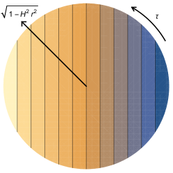
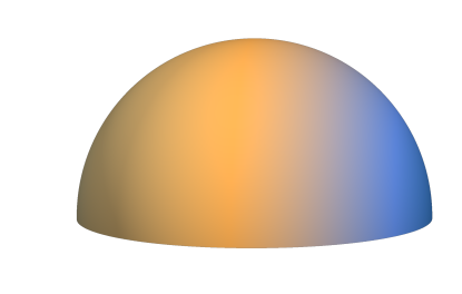
Figure 1: The lowest lying eigenfunction ($\beta=4$), shown both as a projection onto the plane, and also with the hemispherical geometry of the $\tau-r$ $(\tilde{\tau}-x)$ section that makes a stronger link to the global analytic continuation (although here the radius of the suppressed $S^{2}$ is actually zero on the equator!)

Figure 2: The first harmonic eigenfunction ($\beta=10$). On the left and in the middle are the two eigenfunctions, $P_{3}^{0}(x)/x$ and $P_{3}^{2}(x)$cos$(2\tilde{\tau})$. On the right is the combination of the two eigenfunctions that represents the transformed Gegenbauer solution from Hackworth:2004xb .

Finally, we briefly mention the physical interpretations for $\delta\phi_{S}$ and $\delta\phi_{G}$. According to the arguments in Gomberoff:2005je ; Brown:2007sd ; Masoumi:2012yy ; Ai:2018rnh , a static solution in the static patch may be regarded as a thermal transition (thermalon), although the solution in the global patch that is no longer “static” has the interpretation of a quantum tunneling event. Based on this discussion, we would argue that the static patch $\delta\phi_{S}$ may describe a thermal transition inside the cosmological horizon. (Extension to SdS space is provided in Sec. 3.) In addition, a thermal system is an ensemble state of energy and a thermalon would be suppressed by the Boltzmann factor $e^{-\Delta F/T}$, where $\Delta F$ is the change of free energy and $T$ is a temperature. In our situation, the internal energy vanishes due to the Hamiltonian constraint and $\Delta F=-T\Delta{\cal S}$, which leads to the entropic Boltzmann factor (2). This picture is based on an excitation transition and a metastability of initial state, that is guaranteed by the existence of one and only one negative mode, may be not necessary. Indeed, it was shown that a bounce solution with $N$ oscillations has $N$ negative modes in dS background Lavrelashvili:2006cv ; Battarra:2012vu . We do not have any conclusive argument regarding the role of the negative modes in thermal transition and it is an interesting open question.

2.2 Thermalons near the Nariai limit

Having verified that the static patch analysis in Euclidean dS, which may be viewed as the $M\to 0$ limit of SdS, gives equivalent results to the global $O(4)$ analysis, we now present another limit in which we can analytically explore bounce solutions: the Nariai limit Nariai:1 ; Nariai:2 . The SdS spacetime has two horizons: the BH and the cosmological event horizons, whose radii are denoted by $r_{h}$ and $r_{c}$ respectively, that translate into two bolts at each end of the Euclidean section. As the mass of the BH is increased, these two horizons move towards each other, until at $GMH=1/\sqrt{27}$, the horizons merge at $r_{h}=r_{c}=1/\sqrt{3}H$. This is the Nariai limit. Near this limit, the $\tau-r$ metric functions can be approximated by quadratic functions, allowing once again a simple perturbation equation for the scalar field with analytic solutions for some eigenvalues. This time however, we do not expect to have time dependent solutions for our scalar field, as the preferred instantons for large BHs are static (at least in the thin wall case) Gregory:2013hja .

First, we write down the metric near the Nariai limit:

$$ds^{2}=3H^{2}(r_{\epsilon}^{2}-\bar{r}^{2})d\tau^{2}+\frac{d\bar{r}^{2}}{3H^{2}(r_{\epsilon}^{2}-\bar{r}^{2})}+R^{2}d\Omega^{2},$$ (23)

where $r_{\epsilon}\equiv(r_{c}-r_{h})/2$, $R\equiv(\sqrt{3}H)^{-1}$, and $\bar{r}\equiv r-R$. Changing the scale of coordinates as before, $x=\bar{r}/\epsilon$ and $\tilde{\tau}=H\tau$, we finally obtain

$$ds^{2}=3r_{\epsilon}^{2}(1-x^{2})d\tilde{\tau}^{2}+\frac{dx^{2}}{3H^{2}(1-x^{2})}+R^{2}d\Omega^{2},$$ (24)

for which the equation of motion of a massless scalar field is

$$(1-x^{2})\delta\phi^{\prime\prime}-2x\delta\phi^{\prime}+\frac{\beta}{3}\delta\phi\approx 0.$$ (25)

Thus, once again, the perturbation equation for the scalar reduces to a Legendre equation, although this time without any transformation on $\delta\phi$. Note also that now the equation is valid in the range $x\in[-1,1]$, as the range of the $\bar{r}$ coordinate is $[-\epsilon,\epsilon]$. The solution is

$$\delta\phi=P_{\nu}(x),$$ (26)

where $\beta=3\nu(\nu+1)$, and the boundary condition at each horizon is simply that

$$\delta\phi^{\prime}(\pm 1)=\pm\frac{\beta}{6}\delta\phi(\pm 1)=\pm\frac{\nu(\nu+1)}{2}\delta\phi(\pm 1),$$ (27)

which are satisfied for all $\nu$. The lowest eigenfunction with $\nu=1$, corresponds to a solution interpolating between $T\to F$ from the black hole to the cosmological horizon. This solution has $\beta=6$, and we label it as a fundamental mode, or $k=1$.

Let us now consider what happens to this fundamental mode as we move away from the Nariai limit. Naturally, the analytic approximation above becomes less valid, as the cubic nature of the Newtonian potential comes into play. Qualitatively however, we expect that there will still exist a fundamental solution interpolating from ‘$T$’ at $r_{h}$ to ‘$F$’ near $r_{c}$. As we gradually switch off the mass, what remains will be a solution interpolating from ‘$T$’ at $r=0$ to ‘$F$’ at $r_{c}=1/H$; this however is none other than the solution $P_{3}^{0}(x)/x$ illustrated on the left in FIG. 2. In other words, our fundamental mode has continued to the first harmonic in the static patch, moreover, the value of $\beta$ has increased from $\beta_{N}=6$ to $\beta_{dS}=10$. We will therefore be looking for confirmation of this drift of $\beta$ with $M$ in the full numerical calculation.

3 Oscillating bounce in general SdS space

In this section, we will numerically investigate oscillating bounce solutions in the general SdS background. We solve the full Einstein-scalar equations, thus taking account of the gravitational backreaction of the bounce on the background spacetime. We will show that the mass of a seed BH, $M_{+}$, and the curvature of the potential at the top of the barrier, $\beta$, determine the maximum number of possible oscillations of the bounce. An oscillating bounce with a large number of oscillations has a super-thick bubble wall, which can be regarded as an up tunneling, such as the HM transition, around a BH. An interpretation of the oscillating bounce around a BH will be discussed in the next section in more detail.

3.1 Methodology

For simplicity, we use the following effective potential throughout the manuscript

$$V(\phi)=\beta H^{2}\left(-\frac{1}{2}\phi^{2}-\frac{g}{3v}\phi^{3}+\frac{1}{4v^{2}}\phi^{4}\right)+V_{\rm top},$$ (28)

where $H^{2}=(8\pi G/3)V_{\rm top}$ and $\beta=|V^{\prime\prime}(\phi_{\rm top})|/H^{2}$. The potential is constructed so that it’s local maximum, $V_{\rm top}$ is at $\phi=0$ and the true and false vacuum states are at $\phi=\phi_{T}\equiv\frac{v}{2}(g+\sqrt{4+g^{2}})$ and $\phi=\phi_{F}\equiv-\frac{v}{2}(\sqrt{4+g^{2}}-g)$, respectively. We take $V_{\rm top}=10^{-4}M_{\text{Pl}}^{4}$, $\beta\leq 250$, $g=1/\sqrt{8}$, and $v=0.01M_{\text{Pl}}$ throughout the manuscript (FIG. 3).

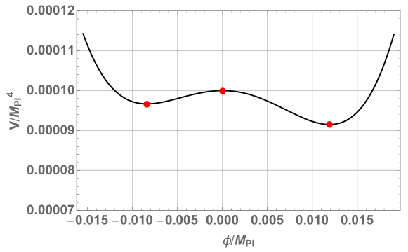
Figure 3: Plot of the effective potential $V(\phi)$ with $V_{\rm top}=10^{-4}M_{\text{Pl}}^{4}$, $\beta=250$, $g=1/\sqrt{8}$, and $v=0.01M_{\text{Pl}}$. Red points show the false vacuum, true vacuum, and the top of barrier.

We consider a phase transition from a uniform configuration of the scalar field $\phi=\phi_{F}$ with a seed BH of mass $M_{+}$ to a spherical and inhomogeneous configuration. In the background of a BH, $O(4)$ symmetry is broken to $O(3)\times U(1)$, and in the following we investigate oscillating bounces preserving this symmetry.

To construct a static bounce around a BH, we assume a spherically symmetric geometry whose generic (Euclidean) metric has the form of

$$ds^{2}=f(r)e^{2\delta(r)}d\tau^{2}+\frac{dr^{2}}{f(r)}+r^{2}(d\theta^{2}+\sin^{2}{\theta}d\varphi^{2}),$$ (29)

where the metric function $f(r)$ is defined as

$$f=1-\frac{2G\mu(r)}{r}.$$ (30)

We have to numerically solve the Einstein and scalar equations simultaneously in order to determine the functions $\mu(r)$, $\delta(r)$ and $\phi(r)$:

$$f\phi^{\prime\prime}+f^{\prime}\phi^{\prime}+\frac{2}{r}f\phi^{\prime}+\delta^{\prime}f\phi^{\prime}-V_{\phi}=0,$$ (31)

$$\mu^{\prime}=4\pi r^{2}\left(\frac{1}{2}f\phi^{\prime}{}^{2}+V\right),$$ (32)

$$\delta^{\prime}=4\pi Gr\phi^{\prime}{}^{2},$$ (33)

where a prime denotes the derivative with respective to $r$. Note that we can eliminate $\delta^{\prime}$ from (31) using (33), meaning that we solve first for $\phi$ and $\mu$, then recover $\delta$ from (33). In the following calculation we use the tortoise coordinate $r^{\ast}$ instead of $r$ since the behavior of the scalar field near a horizon is clearer in this coordinate:

$$dr^{\ast}\equiv\frac{dr}{f(r)}.$$ (34)

Using the tortoise coordinate, (31) and (32) reduce to

$$\frac{d^{2}\phi}{dr^{\ast}{}^{2}}+f(r)\frac{2}{r}\frac{d\phi}{dr^{\ast}}+4\pi Gf^{-1}(r)r\left(\frac{d\phi}{dr^{\ast}}\right)^{3}-f(r)V_{\phi}=0,$$ (35)

$$\frac{d\mu}{dr^{\ast}}=4\pi r^{2}\left(\frac{1}{2}\left(\frac{d\phi}{dr^{\ast}}\right)^{2}+f(r)V\right).$$ (36)

In order for the third term in (35) to be regular at the BH horizon and at the cosmological horizon ($r^{\ast}\to\pm\infty$), we have to impose boundary conditions:

$$\frac{d\phi}{dr^{\ast}}\to 0\ \text{for}\ r^{\ast}\to\pm\infty.$$ (37)

We additionally impose

$$\lim_{r^{\ast}\to-\infty}\mu(r^{\ast}) =\mu_{-},$$ (38)

$$\displaystyle\lim_{r^{\ast}\to\infty}\phi(r^{\ast}) =\phi_{F},$$ (39)

where $\mu_{-}$ is a constant to be determined freely. Note that $\mu_{-}$ is not the “mass” of the remnant BH per se, as it includes the contribution from the cosmological constant to the potential $f$. The metric function in the vicinity of the horizon is matched with that of the SdS metric using the boundary condition (37), which leads to

$$f(r_{h})=1-\frac{2GM_{-}}{r_{h}}-\frac{8\pi G}{3}V(\phi_{h})r_{h}^{2}=1-\frac{2G\mu_{-}}{r_{h}}\ \text{for}\ r^{\ast}\to-\infty,$$ (40)

$$\longrightarrow\mu_{-}=M_{-}+\frac{4\pi}{3}r_{h}^{3}V(\phi_{h}),$$ (41)

where $r_{h}$ denotes the radius of the remnant BH horizon and $\displaystyle\phi_{h}\equiv\lim_{r^{\ast}\to-\infty}\phi$.

On the other hand, one can obtain the total ‘mass’ function inside the cosmological horizon as

$$\mu_{+}\equiv\lim_{r^{\ast}\to\infty}\mu(r^{\ast}).$$ (42)

As before, this is a combination of black hole and cosmological constant terms:

$$\mu_{+}=M_{+}+\frac{4\pi}{3}r_{c}^{3}V(\phi_{F}).$$ (43)

For our solutions, we require that $\mu_{+}$ is the same before and after the phase transition, giving a one-to-one correspondence between $M_{-}$ and $M_{+}$ for a given number of oscillations $k$.

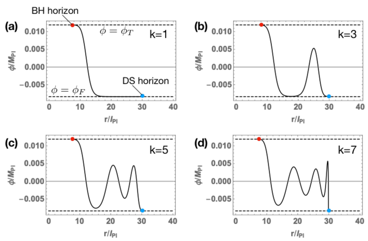
Figure 4: Bounce solutions for $k=1,3,5,$ and $7$ with $\beta=250$ and $(G^{3}V_{\text{top}})^{1/2}\mu_{-}=0.04$. Red and Blue points denote the BH and cosmological horizons, respectively.

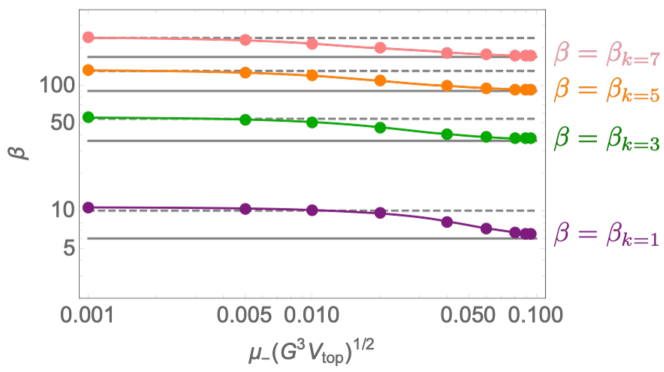
Figure 5: Plot of $\beta_{k=1,3,5,7}$ above which there exist the oscillating bounces with $k$ oscillations. Solid and dashed gray lines show the values of $\beta_{k}$ analytically obtained in the Nariai and dS limits, respectively. Both are well consistent with the numerical results.

Using a shooting method, we numerically calculated the bounce solutions, finding oscillating solutions in which $\phi$ crosses the top of the potential barrier $k$-times ($k\geq 1$) (FIG. 4). Tuning the value of $\phi_{h}$, we can obtain solutions with $k=1$, $3$, $5$, and $7$ in the case of $\beta=|V^{\prime\prime}(\phi_{\rm top})|/H^{2}=250$. It is interesting to consider the reason why $\phi$ can have such an oscillatory behavior. To construct a bounce solution, we have to solve the field equation (35), which can be thought of as classical motion of a particle in the inverted potential via the usual Coleman interpretation. The field $\phi$ starts to roll down from $\phi\simeq\phi_{T}$ at $r=r_{h}$ aiming for $\phi=\phi_{F}$. If the field does not have “enough energy” to reach $\phi_{F}$ in the intermediate region ($r_{h}<r<r_{c}$) it will oscillate, however, as the cosmological horizon is approached, the potential slope becomes very shallow due to $f(r)\to 0$ in the vicinity of $r\simeq r_{c}$, thus allowing $\phi\to\phi_{F}$ in the vicinity of the cosmological horizon $r^{\ast}\to+\infty$.

3.2 Results

We show the dependence of the maximum number of $k$ on $\beta$ and $\mu_{-}$ in FIG. 5. When the curvature at the top of the potential, $\beta$, is much smaller than unity, the only allowed solution is the HM bounce, and oscillating and monotone bounces are not allowed. The oscillating bounce with $k$-times crossing is allowed for $\beta\geq\beta_{k}$ as is shown in FIG. 5. The HM bounce always allowed in principle, but the bounce solutions with $k=1,3,5...$ are limited by $\beta\geq\beta_{k}$. The numerically obtained $\beta_{k}$ is pleasingly consistent with the analytically obtained lower bounds $\beta_{k}\geq 2k(2k+3)$ (gray dashed lines in FIG. 5) and $\beta_{k}\geq 3k(k+1)$ (gray solid lines in FIG. 5) in the dS limit and Nariai limit, respectively. We also compared the analytic solutions obtained by the background geometries, (12) and (26), and the numerical solutions. Then we confirmed that numerical solutions are in good agreement with the analytic solutions expressed by the Legendre equation (see FIG. 7 and FIG. 7 for the dS and Nariai limit, respectively). We should note that we relaxed the boundary condition (39) in the numerical results shown in FIG. 7 and 7.

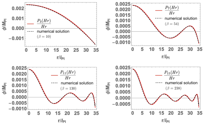
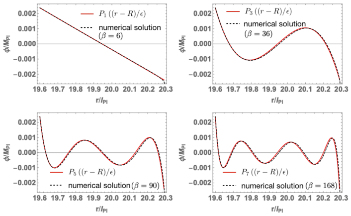
Figure 6: Comparison between the numerically obtined oscillating bounce solutions (black dashed) and analytic solutions in the dS limit (red solid).

Figure 7: Comparison between the numerically obtined oscillating bounce solutions (black dashed) and analytic solutions in the Nariai limit (red solid).

We also investigate the change of BH mass before and after the phase transition for $k=1,3,5$, and $7$ (FIG. 8). Since the oscillating bounce with a higher value of $k$ gives a thicker bubble wall, a larger amount of BH mass is consumed to balance the increment of the total vacuum energy inside the cosmological horizon. However, there is not enough “room” to oscillate and to excite the vacuum energy in the Nariai limit, and so the change of the BH mass is suppressed in the limit.

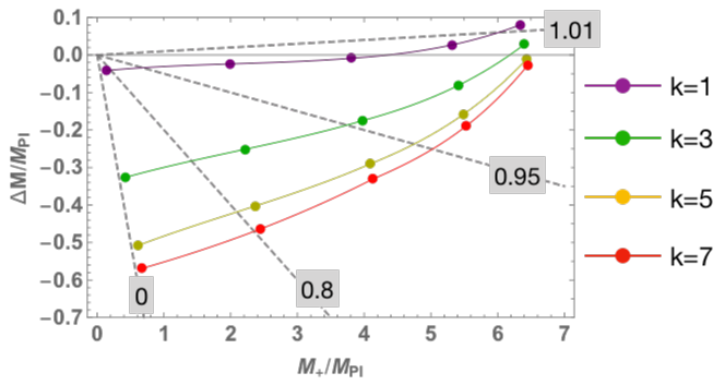
Figure 8: Plot of the mass change $\Delta M=M_{-}-M_{+}$ with $\beta=250$ due to the phase transition. Gray dashed lines show $M_{-}/M_{+}=0,0.8,0.95,$ and $1.01$. The Nariai limit is at $M_{+}\simeq 6.7M_{\text{Pl}}$ in our setup.

4 Hawking-Moss and Oscillating bounces around a BH

The most important similarity between the oscillating bounce and HM bounce is the up-tunneling of matter fields since the oscillating bounce with a large $k$ has a very thick bubble wall dominated by the energy density at the top of the barrier (see FIG. 9). The main difference is that the pure HM instanton represents a jump in the global geometry due to the transition to the top of the potential, which in turn results in a different cosmological horizon area. Once there is a BH however, it is now possible for the HM bounce to have the same cosmological horizon geometry. In this section, we show that the transition rate of oscillating bounces is in good agreement with that of this type of HM bounce around a BH. In Sec. 4.1 we discuss the HM bounce around a BH with fixed horizon geometry (hereafter referred to as the fixed black hole Hawking-Moss (BHHM) bounce) and then we compare the oscillating bounce and BHHM bounce in Sec. 4.2.

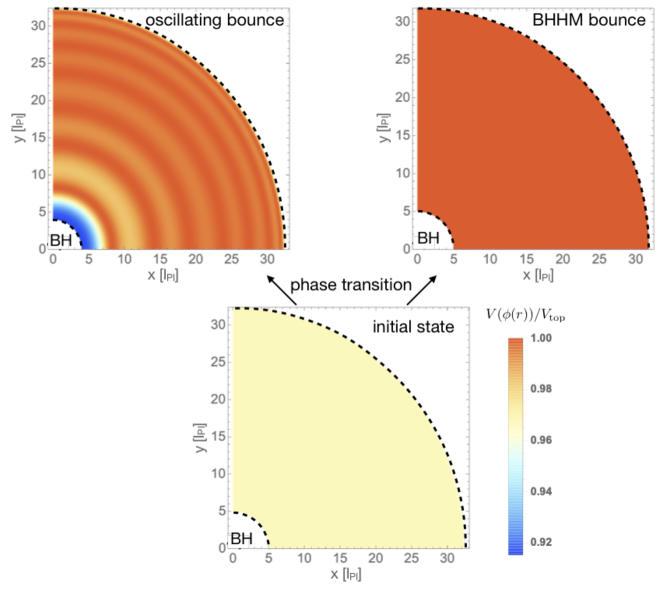
Figure 9: The vacuum energy density profiles (color shows the value of $V(\phi(r))/V_{\text{top}}$) of the oscillating bounce ($k=7$), BHHM bounce, and the initial state. Dashed lines denote the BH and cosmological horizons. We set $\beta=250$ and $\mu_{-}(G^{3}V_{\rm top})^{1/2}=0.02$.

4.1 HM bounce in the presence of a BH

The HM bounce is a thermal transition of homogeneous dS space. Since a thermal state is an ensemble state of energy, up-tunneling is possible and its transition rate is suppressed by the Boltzmann factor. The HM bounce is very similar to this thermal transition and its decay rate can be also approximated by the Boltzmann factor

$$\Gamma\sim e^{-3/(8G^{2}V_{\rm min})+3/(8G^{2}V_{\rm top})}\simeq e^{-\Delta M_{\rm v}/T_{\rm ds}},$$ (44)

where $V_{\rm min}$ and $V_{\rm top}$ denote the vacuum energy densities at a local minimum and top of potential, respectively, $\Delta M_{\rm v}\approx(4\pi/3)(V_{\rm top}-V_{\rm min})/H^{3}$ is notionally the mass-energy inside the cosmological horizon, and $T_{\rm ds}\approx H/2\pi$ is the mean de Sitter temperature (assuming $V_{\rm min}\simeq V_{\rm top}$).

Eq. (44) means that the HM transition is suppressed by the increment of the total mass of vacuum energy, and this feature is very important when extending it to up-tunneling with a BH. This increment consists of both the BH and vacuum energy, and so the up-tunneling rate should be suppressed by the increment of the total mass of both the BH and vacuum energy. If so, the up-tunneling rate may be enhanced when the decrement of the BH mass almost cancels out the increment of the vacuum energy. Recall, the fixed BHHM transition has an up-tunneling of vacuum energy while the total energy inside the cosmological horizon is conserved, i.e. the cosmological radii before and after the BHHM transition match:

$$1-\frac{2GM_{+}}{r_{c}}-\frac{8\pi GV_{\rm min}}{3}r_{c}^{2}=0,$$ (45)

$$1-\frac{2GM_{-}}{r_{c}}-\frac{8\pi GV_{\rm top}}{3}r_{c}^{2}=0.$$ (46)

Then one can obtain the following relations

$$M_{+}+\frac{4\pi}{3}r_{c}^{3}V_{\rm min}=M_{-}+\frac{4\pi}{3}r_{c}^{3}V_{\rm top},$$ (47)

$$\Delta M_{\rm bh}\equiv M_{-}-M_{+}=\frac{4\pi}{3}r_{c}^{3}(V_{\rm top}-V_{\rm min})\equiv-\Delta M_{\rm v},$$ (48)

where $r_{c}$ is the cosmological radius. Hence the mass of a remnant BH is uniquely determined given the values of $V_{\rm top}$, $V_{\rm min}$, and $M_{+}$. One can also read that the total mass is conserved from (48).

The decay rate of the BHHM bounce is obtained from the difference of the Bekenstein-Hawking entropy between the initial and final SdS vacua Gregory:2013hja ; Oshita:2016oqn . The radii of the BH and cosmological horizons before and after the transition are given by

$$r_{h\pm}=\frac{2}{\sqrt{3}H_{\pm}}\cos{\left(\frac{\pi+\cos^{-1}(3\sqrt{3}GM_{\pm}H_{\pm})}{3}\right)},$$ (49)

$$r_{c\pm}=\frac{2}{\sqrt{3}H_{\pm}}\cos{\left(\frac{\pi-\cos^{-1}(3\sqrt{3}GM_{\pm}H_{\pm})}{3}\right)},$$ (50)

respectively, where the suffix of $+$ ($-$) denotes the quantities before (after) the BHHM transition and $r_{c+}=r_{c-}$ is satisfied. When $GM_{\pm}H_{\pm}\ll 1$, one can expand (49) as

$$r_{h\pm} \simeq 2GM_{\pm}+8GM_{\pm}(GM_{\pm}H_{\pm})^{2},$$ (51)

and the difference between the BH horizon area before and after the BHHM transition, $\Delta A$, is approximately given by

$$\Delta A=4\pi(r_{h-}^{2}-r_{h+}^{2})\simeq 16\pi G^{2}(M_{-}^{2}-M_{+}^{2}),$$ (52)

and the change of the Bekenstein-Hawking entropy is

$$\Delta S=\frac{\Delta A}{4G}\simeq 4\pi G(M_{-}^{2}-M_{+}^{2})=\frac{\Delta M_{\rm bh}}{T_{\rm av}}=-\frac{\Delta M_{\rm v}}{T_{\rm av}},$$ (53)

where $T_{\rm av}\equiv 1/(8\pi GM_{\rm av})$, $M_{\rm av}\equiv(M_{+}+M_{-})/2$, and we used (48) in the last equality. Finally, we obtain the decay rate of the BHHM bounce as

$$\Gamma\sim e^{\Delta S}\simeq e^{\Delta M_{\rm bh}/T_{\rm av}}=e^{-\Delta M_{\rm v}/T_{\rm av}}\ \ \text{for}\ \ GM_{\pm}H_{\pm}\ll 1.$$ (54)

Note that the BHHM transition consumes some of the mass of seed BH, therefore there is a threshold of seed mass below which there is no BHHM instanton. This is precisely analogous to the critical seed mass in CDL black hole seeded decay Gregory:2013hja , which is the lowest possible black hole seed that has a static decay instanton.

The lowest seed mass (hereafter referred to as the critical mass), below which the seed BH cannot catalyze the HM transition, can be obtained as follows. Expanding (50) with respect to $GM_{\pm}H_{\pm}$, one obtains

$$r_{\rm c\pm}\simeq\frac{1}{H_{\pm}}(1-GM_{\pm}H_{\pm}),$$ (55)

and requiring the energy conservation, i.e., $r_{\rm c+}=r_{\rm c-}$, one can obtain the following relation

$$\frac{1}{H_{+}}\left(1-GM_{+}H_{+}+{\cal O}((GM_{+}H_{+})^{2})\right)=\frac{1}{H_{-}}\left(1-GM_{-}H_{-}+{\cal O}((GM_{-}H_{-})^{2})\right).$$ (56)

Then the positivity of the remnant mass $(M_{-}\geq 0)$ gives the critical mass of $M_{+}$

$$M_{+}\geq\frac{1}{GH_{+}}-\frac{1}{GH_{-}}\equiv M_{\rm c}\ \ \text{for}\ \ GM_{\pm}H_{\pm}\ll 1.$$ (57)

At the critical mass $M_{+}=M_{\rm c}$, the exponent of the decay rate is simply given by the Bekenstein-Hawking entropy of the seed BH $\Gamma\sim e^{-A/4G}$, where $A$ is the horizon area of the seed BH. In the next subsection, we come back to the oscillating bounce and we show some supporting evidences that the oscillating bounce with many oscillations corresponds to the BHHM bounce.

4.2 Comparison between the oscillating bounce and BHHM bounce

Let us calculate the vacuum decay rate of the oscillating bounce and compare it with that of the fixed BHHM bounce. Since the oscillating bounce is a static solution, its on-shell Euclidean action is minus the Bekenstein-Hawking entropy. Therefore, the exponent of the transition rate is given by the entropy change before and after the phase transition $\Delta{\cal S}$. We numerically calculate $\Delta{\cal S}$ for the oscillating bounce of $k=7$. We find out that the vacuum decay rate for the oscillating bounce is in good agreement with that of the BHHM bounce (FIG. 10), and in the low mass limit ($GM_{+}H_{+}\ll 1$) it is consistent with the Boltzmann factor $e^{\Delta M_{\rm bh}/T_{\rm av}}$. It is also found out that the decay rate of the HM bounce with a BH is highest at the critical mass, for which $\Delta{\cal S}=-A(M_{\rm c})/4G$. Therefore, one can conclude that a smaller seed BH, but larger than the critical mass given in (57), more strongly enhances the HM transition rate, and oscillating bounces with many oscillations is almost identical to the BHHM bounce from the point of view of the vacuum energy density profile (FIG. 9) and of the decay rate (see a red and gray lines in FIG. 10).

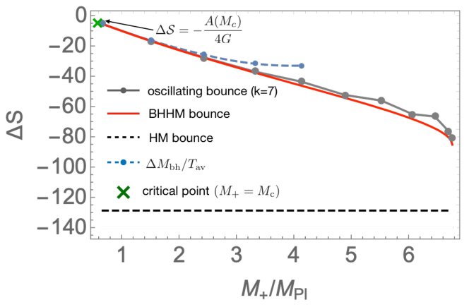
Figure 10: Plot of the entropy change for the oscillating bounce with $k=7$ (grey), BHHM bounce (red) and HM bounce (black dashed), and $\Delta M_{\rm bh}/T_{\rm av}$ (blue). The critical point ($M_{+}=M_{c}\simeq 0.59M_{\rm Pl}$) is marked with the green cross and the Nariai limit is at $M_{+}\simeq 6.7M_{\text{Pl}}$ in our setup. We set $\beta=250$.

5 Conclusion

We investigated the oscillating bounce solutions in the SdS background by using the static patch. We first considered the linearlized equation of motion of the scalar field around the top of the potential and demonstrated that the oscillating bounces in the dS background in both the global and static patches have the same eigenvalue restrictions on $\beta$. This is highly non-trivial since the Wick rotation in the global patch essentially differs from that in the static one. We also analytically obtained the oscillating bounce in the Nariai limit. To extend the bounce solutions to the general SdS case and to take into account the backreaction on spacetime and the non-linear terms in the equation of motion of $\phi$, we numerically solved the Einstein equation and the equation of motion in the spherical and static case. Then we found out that the minimum value of $\beta$ allowing the existence of oscillating bounce with $k$ oscillations at the top of barrier, $\beta_{k}$, is restricted in the range $3k(k+1)\lesssim\beta_{k}\lesssim 2k(2k+3)$, where the lower and upper bounds on $\beta_{k}$ are associated with the Nariai and dS limits, respectively. We also checked the analytic bounce solutions in the dS and Nariai limit are consistent with the numerical solutions.

Since the oscillating bounce with many oscillations has its thick wall, it is natural to expect that such an oscillating bounce may be regarded as an intermediate bounce between the BHHM and static monotone ($k=1$) bounces around a BH. To check this, we estimated the action for the BHHM bounce and found out that it is consistent with the action of an oscillating bounce with many oscillations (comparison with $k=7$ is shown in FIG. 10). Remarkably, the BHHM transition rate is much higher than the HM transition rate without BH (black dashed line in FIG. 10). Note that the BH mass should be smaller than the Nariai mass and larger than the critical mass given in (57). Therefore, we can conclude that a BH in the range of $1/G(H_{+}^{-1}-H_{-}^{-1})<M_{+}<(\sqrt{27}GH_{-})^{-1}$ would catalyze the HM transition, and this effect is significant for small BHs close to the critical limit $M_{+}\gtrsim M_{c}$.

The fact that there is a critical mass, below which the fixed BHHM instantons do not exist is reminiscent of the situation with BH bounces Gregory:2013hja , where there is critical mass below which static BH bounce solutions do not exist. In that case, the mass gap was completed by having CDL-type instantons with no remnant mass. We plan to explore a wider class of instantons beyond the fixed BHHM instantons considered here in the context of the oscillating bounce solutions.

- (1) S. Coleman, Fate of the false vacuum: Semiclassical theory, Phys.Rev. D15 (1977) 2929–2936.
- (2) C. G. Callan and S. Coleman, Fate of the false vacuum II: First quantum corrections, Phys.Rev. D16 (1977) 1762–1768.
- (3) S. Coleman and F. De Luccia, Gravitational effects on and of vacuum decay, Phys.Rev. D21 (1980) 3305–3315.
- (4) R. Gregory, I. G. Moss and B. Withers, Black holes as bubble nucleation sites, JHEP 1403 (2014) 081, [arXiv:1401.0017 [hep-th]].
- (5) P. Burda, R. Gregory and I. Moss, Gravity and the stability of the Higgs vacuum, Phys. Rev. Lett. 115, 071303 (2015) [arXiv:1501.024937 [hep-th]].
- (6) P. Burda, R. Gregory and I. Moss, Vacuum metastability with black holes, JHEP 1508, 114 (2015) [arXiv:1503.07331 [hep-th]].
- (7) P. Burda, R. Gregory and I. Moss, The fate of the Higgs vacuum, JHEP 1606, 025 (2016) [arXiv:1601.02152 [hep-th]].
- (8) K. Mukaida and M. Yamada, False Vacuum Decay Catalyzed by Black Holes, Phys. Rev. D 96 (2017) no.10, 103514 [arXiv:1706.04523 [hep-th]].
- (9) N. Oshita, K. Ueda and M. Yamaguchi, Vacuum decays around spinning black holes, JHEP 2001, 015 (2020) [arXiv:1909.01378 [hep-th]].
- (10) I. Koga, S. Kuroyanagi and Y. Ookouchi, Instability of Higgs Vacuum via String Cloud Phys. Lett. B 800 (2020) 135093 [arXiv:1910.02435 [hep-th]].
- (11) N. Oshita, M. Yamada and M. Yamaguchi, Compact objects as the catalysts for vacuum decays, Phys. Lett. B 791 (2019) 149 [arXiv:1808.01382 [gr-qc]].
- (12) W. A. Hiscock, Can black holes nucleate vacuum phase transitions?, Phys.Rev. D35 (1987) 1161–1170.
- (13) V. Berezin, V. Kuzmin, and I. Tkachev, O(3) invariant tunneling in general relativity, Phys.Lett. B207 (1988) 397.
- (14) V. A. Berezin, V. A. Kuzmin and I. I. Tkachev, Black holes initiate false vacuum decay, Phys. Rev. D 43, 3112 (1991).
- (15) S. W. Hawking and I. G. Moss, Supercooled Phase Transitions in the Very Early Universe, Phys. Lett. 110B, 35 (1982) [Adv. Ser. Astrophys. Cosmol. 3, 154 (1987)].
- (16) J. B. Hartle and S. W. Hawking, Wave Function of the Universe Phys. Rev. D 28 (1983) 2960 [Adv. Ser. Astrophys. Cosmol. 3 (1987) 174]
- (17) A. A. Starobinsky, Stochastic De Sitter (inflationary) Stage In The Early Universe Lect. Notes Phys. 246 (1986) 107.
- (18) A. R. Brown and E. J. Weinberg, Thermal derivation of the Coleman-De Luccia tunneling prescription, Phys.Rev. D76 (2007) 064003, [arXiv:0706.1573 [hep-th]].
- (19) J. C. Hackworth and E. J. Weinberg, Oscillating bounce solutions and vacuum tunneling in de Sitter spacetime, Phys. Rev. D 71, 044014 (2005) [hep-th/0410142].
- (20) E. J. Weinberg, New bounce solutions and vacuum tunneling in de Sitter spacetime, AIP Conf. Proc. 805, no. 1, 259 (2005) [hep-th/0512332].
- (21) V. Balek and M. Demetrian, Euclidean action for vacuum decay in a de Sitter universe, Phys. Rev. D 71, 023512 (2005) [gr-qc/0409001].
- (22) L. Battarra, G. Lavrelashvili and J. L. Lehners, Zoology of instanton solutions in flat potential barriers, Phys. Rev. D 88, 104012 (2013) [arXiv:1307.7954 [hep-th]].
- (23) S. Kanno and J. Soda, Exact Coleman-de Luccia Instantons, Int. J. Mod. Phys. D 21, 1250040 (2012) [arXiv:1111.0720 [hep-th]].
- (24) M. Demetrian, False vacuum decay with gravity in a critical case, Int. J. Theor. Phys. 46, 652 (2007) [gr-qc/0504133].
- (25) S. Stopyra, Standard Model Vacuum Decay with Gravity, Ph. D. thesis.
- (26) A. Rajantie and S. Stopyra, Standard Model vacuum decay with gravity, Phys. Rev. D 95 (2017) no.2, 025008 [arXiv:1606.00849 [hep-th]].
- (27) A. Joti, A. Katsis, D. Loupas, A. Salvio, A. Strumia, N. Tetradis and A. Urbano, (Higgs) vacuum decay during inflation, JHEP 1707 (2017) 058 [arXiv:1706.00792 [hep-th]].
- (28) G. Lavrelashvili, The Number of negative modes of the oscillating bounces, Phys. Rev. D 73, 083513 (2006) [gr-qc/0602039].
- (29) B. H. Lee, W. Lee and D. h. Yeom, Oscillating instantons as homogeneous tunneling channels, Int. J. Mod. Phys. A 28, 1350082 (2013) [arXiv:1206.7040 [hep-th]].
- (30) B. H. Lee, W. Lee, D. Ro and D. h. Yeom, Oscillating Fubini instantons in curved space, Phys. Rev. D 91 (2015) no.12, 124044 [arXiv:1409.3935 [hep-th]].
- (31) N. Oshita and J. Yokoyama, Entropic interpretation of the Hawking–Moss bounce, PTEP 2016, no. 5, 053E02 (2016) [arXiv:1603.06671 [hep-th]].
- (32) I. G. Moss, Black Hole Bubbles, Phys. Rev. D 32 (1985) 1333.
- (33) A. Flachi and T. Tanaka, Chiral Phase Transitions around Black Holes, Phys. Rev. D 84 (2011) 061503 [arXiv:1106.3991 [hep-th]].
- (34) N. Oshita and J. Yokoyama, Phys. Lett. B 785 (2018) 197 [arXiv:1601.03929 [gr-qc]].
- (35) H. Nariai, On a new cosmological solution of Einstein’s field equations of gravitation, Sci. Rep. Tohoku Univ. Ser. 1, (1951). Gen. Rel. Grav., 31, 963-971 (1999).
- (36) H. Nariai, On some static solutions of Einstein’s gravitational field equations in a spherically symmetric case, Sci. Rep. Tohoku Univ. Eighth Ser., (1950). Gen. Rel. Grav., 31, 951-961 (1999).
- (37) A. Gomberoff, M. Henneaux and C. Teitelboim, Decay of the cosmological constant: Equivalence of quantum tunneling and thermal activation in two spacetime dimensions, Phys. Rev. D 71, 063509 (2005) [hep-th/0501152].
- (38) A. Masoumi and E. J. Weinberg, Bounces with O(3) x O(2) symmetry, Phys. Rev. D 86, 104029 (2012) [arXiv:1207.3717 [hep-th]].
- (39) W. Y. Ai, Correspondence between Thermal and Quantum Vacuum Transitions around Horizons, JHEP 1903, 164 (2019) [arXiv:1812.06962 [hep-th]].
- (40) L. Battarra, G. Lavrelashvili and J. L. Lehners, Negative Modes of Oscillating Instantons, Phys. Rev. D 86 (2012), 124001 [arXiv:1208.2182 [hep-th]].