Cosmological models with asymmetric quantum bounces

Abstract

In quantum cosmology, one has to select a specific wave function solution of the quantum state equations under consideration in order to obtain concrete results. The simplest choices have been already explored, in different frameworks, yielding, in many cases, quantum bounces. As there is no consensually established boundary condition proposal in quantum cosmology, we investigate the consequences of enlarging known sets of initial wave functions of the universe, in the specific framework of the Wheeler-DeWitt equation interpreted along the lines of the de Broglie-Bohm quantum theory, on the possible quantum bounce solutions which emerge from them. In particular, we show that many asymmetric quantum bounces are obtained, which may incorporate non-trivial back-reaction mechanisms, as quantum particle production around the bounce, in the quantum background itself. In particular, the old hypothesis that our expanding universe might have arisen from quantum fluctuations of a fundamental quantum flat space-time is recovered, within a different and yet unexplored perspective.

I Introduction

According to the Penrose-Hawking singularity theorems in General Relativity penrose-hawking , the universe has a beginning described by a singularity in space-time, which is outside the scope of the theory and, hence, cannot be investigated. This led to the idea that, in this extreme domain, characterized by very high energy densities and curvature, General Relativity must undergo modifications, which may be due to quantum gravitational effects. Therefore, it is necessary to formulate a quantum theory of gravity to describe the domain previously held as a singularity.

Quantum Mechanics, on the other hand, is understood as a fundamental theory able to describe any physical system, including the whole universe. However, the Copenhagen interpretation cannot be applied to cosmology. The reason is that, in order to solve the measurement problem, this interpretation postulates that the wave function collapses when an observer performs a measurement on the system. Thus an external classical domain is required to perform the collapse of the wave function.

There are some proposals to circumvent this conceptual problem, the most famous being the Many-Worlds interpretation many-worlds , the spontaneous collapse approach spontaneous-collapse , and the de Broglie-Bohm quantum theory Bohm:1951xw ; Bohm:1951xx . We will adopt this last one, a deterministic interpretation in which real trajectories in the configuration space exist. The probabilistic character of Quantum Mechanics is due to the existence of hidden variables (initial field configurations), and arises statistically. In this theory, the collapse of the wave function is effective: the system occupies one of the branches of the wave function, and the others remain empty and incommunicable to each other. Therefore, an external observer is no longer needed, and we achieve the conceptual coherence necessary to apply this approach to cosmology.

The quantum cosmological models that arise from this approach enable the avoidance of the initial singularity, giving rise to a bounce Pinto-Neto:2013toa ; PintoNeto:2004uf , or even multiple bounces Peter:2016kan ; Bacalhau:2017qnu , which are preceded by a contraction of the scale factor and followed by an expanding phase.

In this paper, we consider generalizations of the quantum cosmological models found in Refs Pinto-Neto:2013toa ; PintoNeto:2004uf arising from the Wheeler-DeWitt quantization of the background, which are symmetric around the bounce, obtained from enlarged prescriptions for the initial wave function. Our aim is to obtain asymmetric bounces, capable to describe non-linear back-reactions coming from particle production around the bounce, which can alter the background evolution in the expanding phase. Indeed, taking into account generalizations of the initial Gaussian wave functions considered in Refs Pinto-Neto:2013toa ; PintoNeto:2004uf , we were able to obtain a variety of asymmetric quantum bounce trajectories in different contexts, with quite interesting properties, as it will be discussed in the sequel.

The paper is divided as follows: in the next section we present the mini-superspace model in which the de Broglie-Bohm quantization will be implemented, and the standard symmetric quantum bouncing trajectories obtained from initial Gaussian wave functions centered at the origin, and without phase velocity. The unique free parameter (besides the initial values of the trajectories), is the standard deviation of the Gaussian. In section III, we enlarge the set of initial wave functions by considering initial Gaussians, also centered at the origin, with phase velocity, hence adding a new parameter to the system. It is shown that unitary evolution of such initial wave functions continue to yield symmetric quantum bounces. As unitary evolution is not a mandatory requirement for mini-superspace wave functions in the de Broglie-Bohm theory, we gave up with unitarity, obtaining, in this way, asymmetric quantum bounces. In section IV, we enlarge once more the class of initial wave functions by taking superpositions with two more free parameters than the standard deviation of the Gaussian, obtaining asymmetric quantum bounces with unitarity preserved. In the Conclusion, we comment on our results, and discuss future developments.

II De Broglie-Bohm quantization of the mini-superspace Friedmann model

For a flat, homogeneous and isotropic universe filled with a perfect fluid with equation of state $P=\omega\rho$, where $P$ is the pressure, $\rho$ is the energy density and $\omega$ is the equation of state parameter, the ADM Arnowitt:1962hi and the Schutz Schutz:1970my formalisms lead to the following Hamiltonian

$$H=\frac{L_{p}^{2}}{V}NH_{0},$$ (1)

with

$$H_{0}\equiv\frac{P_{T}}{a^{3\omega}}-\frac{P_{a}^{2}}{4a},$$ (2)

where $L_{p}$ is the Planck length, $V$ is the volume of the co-moving homogeneous 3-dimensional hyper-surface, which we are supposing to be compact, $a$ is the scale factor of the universe, $T$ is the parameter related to the degree of freedom of the fluid, which plays the role of time, $P_{a}$ and $P_{T}$ are their respective canonically conjugated momenta, and $N$ is the lapse function. We are using natural units, $\hbar=c=1$, hence all canonical variables above are dimensionless, and the Hamiltonian has dimensions of energy $=1/$length, as it should be. The constant $L_{p}/V$ will be absorbed in the definition of time later on, yielding a dimensionless cosmic time. The Friedmann equations can be readily obtained from the Hamiltonian

$$H=NH_{0},$$ (3)

where N is the lapse function of the ADM formalism. Applying the Dirac quantization procedure for constrained systems, where the wave function is annihilated by the the constraint operator, $\hat{H_{0}}\Psi=0$, and taking into account a particular choice of the factor ordering Halliwell , which leads to a Schrödinger equation with a covariant Laplacian under redefinitions of $a$, we arrive at the following Wheeler-DeWitt equation:

$$i\frac{\partial}{\partial T}\Psi(a,T)=\frac{a^{(3\omega-1)/2}}{4}\frac{\partial}{\partial a}\left[a^{(3\omega-1)/2}\frac{\partial}{\partial a}\right]\Psi(a,T).$$ (4)

Performing the variable transformation given by

$$\chi=\frac{2}{3(1-\omega)}a^{3(1-\omega)/2},$$ (5)

we obtain

$$i\frac{\partial\Psi(\chi,T)}{\partial T}=\frac{1}{4}\frac{\partial^{2}\Psi(\chi,T)}{\partial\chi^{2}},$$ (6)

which can be identified as a Schödinger equation for a free particle of mass $m=2$ in one dimension with the opposite sign of the time derivative term. The solutions of Eq. (6) are the wave functions of the universe. With the choice $N=a^{3\omega}$ for the lapse function, the parameter $T$ relates to the dimensionless cosmic time $t=(L_{p}^{2}/V)t_{c}$ through $dt=a^{3\omega}dT$, where $t_{c}$ is the usual cosmic time, with dimension of length.

Once the scale factor $a$ and, consequently, the variable $\chi$ must assume positive values, we are dealing with a Schrödinger equation for a particle with negative kinetic energy in the half axis Gitman . In order to obtain unitary solutions and, as a consequence, a consistent probabilistic interpretation, it is necessary to perform a self-adjoint extension, that is, to consider the perfectly reflecting boundaries, which are given by the following condition:

$$\left(\Psi^{*}\frac{\partial\Psi}{\partial\chi}-\Psi\frac{\partial\Psi^{*}}{\partial\chi}\right)\Biggr{|}_{\chi=0}=0.$$ (7)

Note, however, that the de Broglie-Bohm quantum theory is a dynamical fundamental theory, where probabilities arise in a secondary step, as in Classical Mechanics. And indeed, a probabilistic interpretation of the wave function of the Universe may not make sense, since there is only one universe in this approach. A probabilistic interpretation is required only for subsystems in the Universe, where we can perform measurements. In this situation, one can use the so called conditional wave functions for subsystems, in which the Wheeler-DeWitt equation reduces to an unitary Schrödinger form, and a probabilistic interpretation where the Born rule is valid can be recovered, which is called quantum equilibrium, see Ref. Falciano:2008nk for details. Of course this opens the possibility that during this process violations of standard quantum mechanics might occur. Unfortunately, almost all systems in Nature have evolved to the quantum equilibrium phase, where the probability distribution is described by $\rho$, see Refs. Val1 ; Val2 for detailed investigations about this process, and possible exceptions. Concluding, in what follows, we will not require unitary evolution as necessary feature of the mini-superspace wave function.

Writing the wave function as $\Psi=Re^{iS}$, and substituting into Eq. (4), we obtain two real equations,

$$\frac{\partial\rho}{\partial T}-\frac{\partial}{\partial a}\left[\frac{a^{(3\omega-1)}}{2}\frac{\partial S}{\partial a}\rho\right]=0$$ (8)

$$\frac{\partial S}{\partial T}-\frac{a^{(3\omega-1)}}{4}\left(\frac{\partial S}{\partial a}\right)^{2}$$

$$+\frac{a^{(3\omega-1)/2}}{4R}\frac{\partial}{\partial a}\left[a^{(3\omega-1)/2}\frac{\partial R}{\partial a}\right]=0,$$ (9)

where $\rho(a,T)=a^{(1-3\omega)/2}|\Psi|^{2}$.

The key feature of the de Broglie-Bohm quantum theory is to assume that positions in configuration space (in our case $a$) have objective reality, independently of any observation, and satisfy the so called guidance equation

$$\dot{a}=-\frac{a^{(3\omega-1)}}{2}\frac{\partial S}{\partial a},$$ (10)

or

$$\frac{d\chi}{dT}=-\frac{1}{2}\frac{\partial S}{\partial\chi}.$$ (11)

With Eq. (10), one can interpret Eq. (8) as a continuity equation for the distribution $\rho$, and Eq. (II) as a generalized Hamilton-Jacobi equation supplemented by the so called quantum potential,

$$Q\equiv-\frac{a^{(3\omega-1)/2}}{4R}\frac{\partial}{\partial a}\left[a^{(3\omega-1)/2}\frac{\partial R}{\partial a}\right].$$ (12)

If one wants to recover the physical dimensions of Eqs. (8) and (II), one can easily verify that Planck constant $\hbar$ re-appears only multiplying the quantum potential, $Q\rightarrow\hbar^{2}Q$. Hence $Q$ brings the quantum effects to the dynamics. Once the total energy given by Eq. (II) includes also the quantum potential $Q$, the trajectory given by Eq. (10) will not be the same as the classical one, unless $Q$ is negligible with respect to the other terms. This effect is responsible for the emergence of the quantum bounce, avoiding the standard classical initial singularity.

Let us consider an initial wave function of the universe given by

$$\Psi_{0}(\chi)=\left(\frac{8}{\pi\sigma^{2}}\right)^{\frac{1}{4}}\exp\left(-\frac{\chi^{2}}{\sigma^{2}}\right),$$ (13)

which satisfies the boundary condition (7). In order to obtain an unitary evolution, we must apply the correspondent propagator to the Wheeler-DeWitt equation (6) considering the boundary condition (7). It means that we must sum two propagators of a Schrödinger equation with negative kinetic energy, one to $\chi_{0}$ and another to $-\chi_{0}$. We then obtain

$$G(\chi,\chi_{0},T) = \sqrt{-\frac{i}{\pi T}}\exp\left[-\frac{i(\chi-\chi_{0})^{2}}{T}\right]$$ (14)

$$+ \sqrt{-\frac{i}{\pi T}}\exp\left[-\frac{i(\chi+\chi_{0})^{2}}{T}\right].$$

The propagator (14) is not the most general one that satisfies the boundary condition (7). One could, for instance, change the relative sign to minus in order to obtain $G(\chi=0)=0$. However, this propagator leads to a trivial solution for the propagated wave function of the universe. Thus, in practice, the propagator that results in a non-trivial solution satisfies a more restrictive boundary condition, which is given by the von Neumann condition $\partial_{\chi}G|_{\chi=0}=0$. Superpositions of the propagators with relative signs plus and minus with a phase difference of $\pm\pi/2$ are also allowed. However, the only difference in the propagated wave function is a factor that does not modify the Bohmian trajectories.

Applying (14) to the initial wave function (13), we arrive at the wave function for all times

$$\Psi(\chi,T)=\left[\frac{8\sigma^{2}}{\pi(\sigma^{4}+T^{2})}\right]^{\frac{1}{4}}\exp\left[-\frac{\sigma^{2}\chi^{2}}{\sigma^{4}+T^{2}}\right]$$

$$\times\exp\left[-i\left(\frac{T\chi^{2}}{\sigma^{4}+T^{2}}+\frac{1}{2}\arctan\left(\frac{\sigma^{2}}{T}\right)-\frac{\pi}{4}\right)\right],$$ (15)

which also satisfies Eq. (7). Using the phase $S$ of the above wave function, we are able to obtain the trajectory of the parameter $\chi$ through Eq. (11). It reads

$$\chi(T)=\chi_{b}\left[1+\left(\frac{T}{\sigma^{2}}\right)^{2}\right]^{\frac{1}{2}},$$ (16)

where $\chi_{b}$ is the value of $\chi$ at the bounce, which occurs at $T=0$. One can re-obtain the classical solution by taking a Gaussian infinitely peaked. In order to do that, one should consider the differential equation with initial condition $\chi_{0}=\chi(T_{0})$, which leads to the solution

$$\chi(T)=\chi_{0}\frac{\sqrt{T^{2}+\sigma^{4}}}{\sqrt{T_{0}^{2}+\sigma^{4}}}.$$ (17)

Then, by making $\sigma^{2}\rightarrow 0$, the classical cosmology given by $\chi(T)=\chi_{0}T/T_{0}$ is obtained.

In terms of the scale factor $a$ one gets,

$$a(T)=a_{b}\left[1+\left(\frac{T}{\sigma^{2}}\right)^{2}\right]^{\frac{1}{3(1-\omega)}},$$ (18)

where $a_{b}$ and $\chi_{b}$ are related also through Eq. (5). Eq. (18) describes a symmetric bounce, which is plotted in figure 1. It tends to the classical solution for large values of $T$.

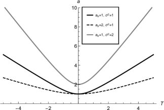
Figure 1: $a$ vs $T$ for $\omega=\frac{1}{3}$.

A good model for the perfect hydrodynamical fluid in the early universe, where all particles are highly relativistic, is a radiation fluid with $w=1/3$, which will be considered from now on. Note that, in this case, $T=\eta$, the conformal time (remember the relation of $T$ with cosmic time $t$, $dt=a^{3w}dT$).

It is convenient to express the bounce solution in terms of cosmological quantities, which is achieved by relating the parameters of the wave function to observables. With this purpose, we will follow the same procedure developed in Celani2017 . We first obtain the Hubble function, given by $H=\frac{\dot{a}}{a}$, where dot denotes the derivative with respect to the physical cosmic time. We then take an expansion of the Hubble function squared for large times $T$, which reads

$$H^{2}=\frac{a_{b}^{2}}{a^{4}\sigma^{4}}=H_{0}^{2}\Omega_{r0}\frac{a_{0}^{4}}{a^{4}},$$ (19)

where in the last equality we used the classical Friedmann equation, yielding

$$\Omega_{r0}=\frac{a_{b}^{2}}{a_{0}^{4}H_{0}^{2}\sigma^{4}},$$ (20)

where $\Omega_{r0}=\rho_{r0}/\rho_{c0}$ is the dimensionless density parameter for radiation today. The subscript ₀ in all quantities indicates their current values. The quantities $\rho_{r0}$ and $\rho_{c0}=3H_{0}^{2}/8\pi G$ are, respectively, the current energy density of radiation and the current critical density.

Performing the following transformation of variables

$$x_{b} = \frac{a_{0}}{a_{b}}$$ (21)

$$\overline{\sigma} = \sigma\sqrt{a_{0}H_{0}},$$ (22)

we obtain

$$\overline{\sigma}^{2}=\frac{1}{x_{b}\sqrt{\Omega_{r0}}}.$$ (23)

In its turn, the curvature scale at the bounce is given by

$$L_{b}=\frac{1}{\sqrt{R}}\bigg{.}\bigg{|}_{T=0}=\frac{\overline{\sigma}^{2}}{\sqrt{6}x_{b}H_{0}}=\frac{1}{x_{b}^{2}H_{0}\sqrt{6\Omega_{r0}}},$$ (24)

where $R$ is the Ricci scalar.

To ensure that the Wheeler-DeWitt equation is a valid approximation for a more fundamental theory of quantum gravity Kiefer , we must require that the bounce scale is larger than the Planck scale, that is $L_{b}>L_{p}$. Taking $H_{0}\approx 70\ km\times s^{-1}\times Mpc^{-1}$, $\Omega_{r0}\approx 10^{-4}$ and given that $L_{p}/R_{H0}\approx 1.25\times 10^{-61}$, where $R_{H0}=1/H_{0}$ is the Hubble radius today, we obtain the upper bound for $x_{b}$

$$x_{b}<1.8\times 10^{31}.$$ (25)

The lower limit can be obtained by requiring that the bounce occurs at energy scales much larger than the nucleosynthesis energy scale, i.e. $T_{BBN}=10$ MeV. Using the CMB temperature equal to $T_{\gamma 0}=2.7\ K$ in Mev, and the linear relation between the temperature and the scale factor

$$\frac{T_{\gamma 0}}{T_{BBN}}=\frac{a_{BBN}}{a_{0}}=x_{BBN}^{-1},$$ (26)

we obtain

$$x_{b}\gg 10^{11}.$$ (27)

III Generalized symmetric bounces and non-unitary asymmetric bounces

III.1 Generalized symmetric quantum bounces

Although the simplicity of the previous symmetric bounce, it represents a fine-tuning in the theory, since the contraction phase is restricted to be the same as the expansion reversed in time. For this reason, we aim to obtain cosmological models with asymmetric trajectories for the scale factor $a$.

Our initial proposal to obtain asymmetric solutions was to include a factor of the form $\exp(ip\chi)$ in the initial wave function, which represents a velocity for the Gaussian proposed in Eq. (13). Thus we have

$$\Psi_{0}(\chi)=\left(\frac{8}{\pi\sigma^{2}}\right)^{\frac{1}{4}}\exp\left(-\frac{\chi^{2}}{\sigma^{2}}+ip\chi\right).$$ (28)

Note that this initial wave function does not satisfy the boundary condition (7), which means that unitarity is not satisfied at $T=0$. However, implementing a convolution between this initial wave function and a propagator that satisfies condition (7), we are, in practice, dealing with the projection of $\Psi_{0}$ onto the subspace of square-integrable functions on the $\chi$ half-line satisfying the von Neumann boundary condition. As a result, the propagated wave function that results from this convolution is going to satisfy (7).

Propagating this initial wave function (28) with the propagator (14) from $0$ to $+\infty$, that is, performing a unitary evolution, we obtain the following wave function for all times:

$$\Psi(\chi,T) = (2\pi\sigma^{2})^{-\frac{1}{4}}\biggl{(}-1+\frac{iT}{\sigma^{2}}\biggl{)}^{-\frac{1}{2}}$$ (29)

$$\times \biggl{[}\phi(\chi,T)+\phi(-\chi,T)\biggr{]},$$

where

$$\phi(\chi,T) \equiv \exp\biggl{[}-\frac{\sigma^{2}\chi^{2}}{T^{2}+\sigma^{4}}-\frac{T(p^{2}T\sigma^{2}-4p\sigma^{2}\chi)}{4(T^{2}+\sigma^{4})}$$ (30)

$$+ i\biggl{(}-\frac{T\chi^{2}}{T^{2}+\sigma^{4}}+\frac{\sigma^{2}(p^{2}T\sigma^{2}-4p\sigma^{2}\chi)}{4(T^{2}+\sigma^{4})}\biggr{)}\biggr{]}$$

$$\times \biggl{(}1-\operatorname{Erf}\left[\epsilon(\chi,T)\right]\biggr{)}$$

and

$$\epsilon(\chi,T)\equiv\biggl{(}\frac{pT}{2}+\chi\biggr{)}\biggl{[}iT\biggl{(}-1+\frac{iT}{\sigma^{2}}\biggr{)}\biggr{]}^{-\frac{1}{2}}.$$ (31)

The wave function (29) satisfies the boundary condition (7). Thus, as mentioned before, the non-unitarity at the point $T=0$ for the initial wave function (28) does not spoil the unitarity after the convolution with the propagator (14).

We can see from Eq. (29) that the wave function was propagated equally to $\chi$ and to $-\chi$. Thus terms and arguments that are linear in $\chi$ are symmetrized with respect to $\chi=0$ by the unitary evolution with the propagator (14).

In order to exemplify a Bohmian trajectory for the scale factor $a$ related to an unitary wave function with factors of the form $\exp(ip\chi)$, we are going to consider only the terms

$$\overline{\Psi}(\chi,T) = (2\pi\sigma^{2})^{-\frac{1}{4}}\biggl{(}-1+\frac{iT}{\sigma^{2}}\biggl{)}^{-\frac{1}{2}}$$ (32)

$$\times \biggl{[}\overline{\phi}(\chi,T)+\overline{\phi}(-\chi,T)\biggr{]},$$

where

$$\overline{\phi}(\chi,T) \equiv \exp\biggl{[}-\frac{\sigma^{2}\chi^{2}}{T^{2}+\sigma^{4}}-\frac{T(p^{2}T\sigma^{2}-4p\sigma^{2}\chi)}{4(T^{2}+\sigma^{4})}$$ (33)

$$+ i\biggl{(}-\frac{T\chi^{2}}{T^{2}+\sigma^{4}}+\frac{\sigma^{2}(p^{2}T\sigma^{2}-4p\sigma^{2}\chi)}{4(T^{2}+\sigma^{4})}\biggr{)}\biggr{]},$$

which also constitutes a unitary solution of the Wheeler-DeWitt equation (6). The choice to disregard the Gauss’s error functions is for the sake of simplicity.

Inserting the global phase $\overline{S}$ of the wave function (32) into Eq. (11), it is possible to obtain a differential equation for the parameter $\chi$. It reads

$$\frac{d\chi}{dT}=\frac{2T\chi\cos\biggl{(}\frac{2p\sigma^{4}\chi}{T^{2}+\sigma^{4}}\biggr{)}+2T\chi\cosh\biggl{(}\frac{2pT\sigma^{2}\chi}{T^{2}+\sigma^{4}}\biggr{)}+pT\sigma^{2}\sin\biggl{(}\frac{2p\sigma^{4}\chi}{T^{2}+\sigma^{4}}\biggr{)}+p\sigma^{4}\sinh\biggl{(}\frac{2pT\sigma^{2}\chi}{T^{2}+\sigma^{4}}\biggr{)}}{2(T^{2}+\sigma^{4})\biggl{[}\cos\biggl{(}\frac{2p\sigma^{4}\chi}{T^{2}+\sigma^{4}}\biggr{)}+\cosh\biggl{(}\frac{2pT\sigma^{2}\chi}{T^{2}+\sigma^{4}}\biggr{)}\biggr{]}}.$$ (34)

Using Eq. (5) in Eq. (34) and solving it numerically with initial condition $a_{i}=a(T_{i})$, we obtain the trajectory of the scale factor $a(T)$, which is plotted in figure 2.

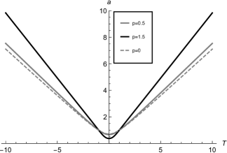
Figure 2: $a$ vs $T$ for $\sigma=1.0$, $a_{i}=1.0$, $T_{i}=1.0$, $\omega=\frac{1}{3}$.

The result is a symmetric bounce, regardless of the value of the parameter $p$ related to the asymmetry. It happens when the unitary evolution for factors of the form $\exp(ip\chi)$ is maintained. As explained before, once these factors are linear in $\chi$ inside the exponential, they are going to be propagated equally to $\chi$ and to $-\chi$, resulting in a symmetrization of the propagated wave function and, as a consequence, of the trajectory of the scale factor $a$.

Note that different symmetric bounces can be obtained in other approaches to quantum cosmology. For instance, in Refs Gryb1 ; Gryb2 , a relational quantization method was implemented, where unitarity is a necessary requirement in order to obtain a consistent probabilistic interpretation, and bouncing models were also found. On the other hand, our work relies on a deterministic interpretation of quantum mechanics, where probabilities are not fundamental, allowing to explore the consequences of wave functions of the Universe which are not restricted to evolve satisfying unitarity requirements.

III.2 Non-unitary asymmetric quantum bounces

An alternative to this hindrance is to give up unitarity, which is allowed according to the discussion previously made. In practise, it means to disconsider the boundary condition (7). The correspondent propagator is then only the first term of the propagator (14), given by

$$G^{NU}(\chi,\chi_{0},T)=\sqrt{-\frac{i}{\pi T}}\exp\left[-\frac{i(\chi-\chi_{0})^{2}}{T}\right],$$ (35)

where $NU$ stands for non-unitary. Applying the propagator (35) to the initial wave function (28) without the normalization factor from $-\infty$ to $+\infty$, we obtain the following wave function for all times:

$$\Psi(\chi,T)=\biggl{(}-1+\frac{iT}{\sigma^{2}}\biggr{)}^{-\frac{1}{2}}\exp\left(\frac{\frac{ip^{2}T}{4}+ip\chi-\frac{\chi^{2}}{\sigma^{2}}}{1-\frac{iT}{\sigma^{2}}}\right).$$ (36)

We take the integration from $-\infty$ to $\infty$ in Eq. (35) in order to avoid terms containing Gauss error functions that arise if the integration is performed from $0$ to $\infty$. In the end we must check that the restriction $\chi>0$ is still staisfied.

Writing Eq. (36) as $\Psi(\chi,T)=R(\chi,T)e^{iS(\chi,T)}$, we obtain

$$\Psi(\chi,T)=\biggr{(}-1+\frac{iT}{\sigma^{2}}\biggl{)}^{-\frac{1}{2}}\overline{\phi}(-\chi,T),$$ (37)

where $\overline{\phi}(\chi,T)$ is given by Eq. (33) (the first factor in the above equation does not depend on $\chi$, hence it does not affect the calculation of the Bohmian trajectories). Then, by inserting $S$ into Eq. (11), it is possible to obtain the trajectory in terms of $\chi$. It reads

$$\chi(T)=\chi_{b}\biggl{[}1+\left(\frac{T}{\sigma^{2}}\right)^{2}+\left(\frac{p}{2\chi_{b}}\right)^{2}(T^{2}+\sigma^{4})\biggr{]}^{\frac{1}{2}}-\frac{pT}{2},$$ (38)

where $\chi_{b}=\chi(T_{b})$ is the value of the variable $\chi$ at the moment of the bounce $T_{b}=\frac{p\sigma^{4}}{2\chi_{b}}$, which is not equal to zero as in the symmetric case. In terms of the scale factor, the trajectory reads

$$a(T) = \Biggl{\{}\Biggr{.}-\frac{3p(1-\omega)}{4}T+a_{b}^{\frac{3(1-\omega)}{2}}\Biggl{[}1+\left(\frac{T}{\sigma^{2}}\right)^{2}$$ (39)

$$+ \left(\frac{3p(1-\omega)}{4}\right)^{2}\frac{(T^{2}+\sigma^{4})}{a_{b}^{3(1-\omega)}}\Biggr{]}^{\frac{1}{2}}\Biggl{.}\Biggr{\}}^{\frac{2}{3(1-\omega)}},$$

where $a_{b}$ relates to $\chi_{b}$ through Eq. (5). The trajectory (39) is shown in figure 3 for $w=1/3$, where it is evidenced that the value of the parameter $p$ is directly related to the intensity of the asymmetry.

Note that Eq. (39) does not admit a singularity or negative values for $a(T)$, since we always have

$$\frac{3p(1-\omega)}{4}T<a_{b}^{\frac{3(1-\omega)}{2}}$$

$$\times\Biggl{[}1+\left(\frac{T}{\sigma^{2}}\right)^{2}+\left(\frac{3p(1-\omega)}{4}\right)^{2}\frac{(T^{2}+\sigma^{4})}{a_{b}^{3(1-\omega)}}\Biggr{]}^{\frac{1}{2}}.$$ (40)

This ensures that the restrictions $\chi>0$ and $a>0$ are satisfied, although we have disregarded the boundary condition (7) and propagated the wave function from $-\infty$ to $\infty$. A bounce solution is naturally obtained, without the need to impose restrictions to recover the positivity of the scale factor.

For $p=0$ we re-obtain the symmetric bounce (18), which makes explicit the relation between the asymmetry and the factor $\exp(ip\chi)$.

As in the symmetric case, the classical solution arises for large values of $T$.

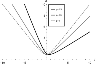
Figure 3: $a$ vs $T$ for $\sigma=1.0$, $a_{b}=1.0$, $\omega=\frac{1}{3}$.

In order to obtain a slope in the contracting phase lower than the slope in the expanding phase, one has to take $p<0$, or, equivalently, to change the factor from $\exp(ip\chi)$ to $\exp(-ip\chi)$ in the initial wave function (28) keeping $p>0$. This case is particularly interesting, once the contraction phase may consist of an almost Minkowski universe. Applying the same procedure to obtain the Bohmian trajectory, we obtain $a$, which is plotted in figure 4.

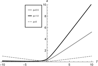
Figure 4: $a$ vs $T$ for $\sigma=1.0$, $a_{b}=0.1$, $\omega=\frac{1}{3}$.

Just as we did for the symmetric case, let us express the wave function parameters in terms of cosmological quantities for the case $w=1/3$. Defining the parameters

$$x_{b} = \frac{a_{0}}{a_{b}}$$ (41)

$$\overline{\sigma} = \sigma\sqrt{a_{0}H_{0}}$$ (42)

$$\overline{p} = \frac{p}{a_{0}^{2}H_{0}}$$ (43)

$$\overline{\eta} = \frac{\eta}{\sigma^{2}}$$ (44)

$$y^{2} = \frac{x_{b}\overline{p}{\overline{\sigma}}^{2}}{2},$$ (45)

one can write

$$a=a_{b}\biggl{(}\pm y^{2}\overline{\eta}+\sqrt{1+y^{4}}\sqrt{1+{\overline{\eta}}^{2}}\biggr{)},$$ (46)

where the $\pm$ signs correspond to wave function phases $\exp(\mp ip\chi)$, with $p\geq 0$. In the limit $|\overline{\eta}|>>1$, we get for the Hubble function,

$$H^{2}=\frac{\biggl{(}\pm y^{2}+\sqrt{1+y^{4}}\biggr{)}^{2}a_{b}^{2}H_{0}^{2}a_{0}^{2}}{{\overline{\sigma}}^{4}a^{4}}=H_{0}^{2}\Omega_{r0}\frac{a_{0}^{4}}{a^{4}},$$ (47)

in the expanding phase, and

$$H^{2}=\frac{\biggl{(}\mp y^{2}+\sqrt{1+y^{4}}\biggr{)}^{2}a_{b}^{2}H_{0}^{2}a_{0}^{2}}{{\overline{\sigma}}^{4}a^{4}}=H_{0}^{2}\Omega_{rc}\frac{a_{0}^{4}}{a^{4}},$$ (48)

in the contracting phase, where $\Omega_{rc}$ is the radiation energy density when the Universe has $H=H_{0}$ in the contracting phase divided by the critical density $\rho_{c}$. These equations imply that

$$\Omega_{r0}=\frac{\left(\pm y^{2}+\sqrt{1+y^{4}}\right)^{2}}{{\overline{\sigma}}^{4}x_{b}^{4}},$$ (49)

$$\overline{\sigma}^{2}=\left[x_{b}^{2}\Omega_{r0}\biggl{(}1\mp\frac{\overline{p}}{\sqrt{\Omega_{r0}}}\biggr{)}\right]^{-1/2},$$ (50)

and

$$\Omega_{rc}=\Omega_{r0}\biggl{(}1\mp\frac{\overline{p}}{\sqrt{\Omega_{r0}}}\biggr{)}^{2}.$$ (51)

Note that the $+$ sign in Eq. (46) implies, from Eq. (50), that $0\leq\overline{p}<\sqrt{\Omega_{r0}}$. From Eq. (51), one can see that $\Omega_{rc}\leq\Omega_{r0}$, and in the limit $\overline{p}\to\sqrt{\Omega_{r0}}$ one has $\Omega_{rc}\to 0$. Hence, the contracting universe can be made arbitrarily flat, and the radiation fluid is created around the quantum phase, during the bounce.

In the $-$ sign case in Eq. (46), there is no constraint in $\overline{p}$, $0\leq\overline{p}<\infty$, and $\Omega_{rc}\geq\Omega_{r0}$.

In this asymmetric case, the maximum curvature does not occur at the bounce, ${\overline{\eta}}_{\rm bounce}\mp y^{2}$, but at the conformal time ${\overline{\eta}}_{\rm max}\mp\sqrt{\frac{\sqrt{1+y^{4}}-1}{2}}$. Hence, the minimum curvature scale reads

$$L_{\rm min} = \frac{1}{\sqrt{R}}\bigg{.}\bigg{|}_{{\overline{\eta}}_{\rm max}}$$ (52)

$$= \frac{R_{H0}\left(1+\sqrt{1\mp\frac{\overline{p}}{\sqrt{\Omega_{r0}}}}\right)^{3}}{8\sqrt{3\Omega_{r0}}x_{b}^{2}\left(1\mp\frac{\overline{p}}{\sqrt{\Omega_{r0}}}\right)^{2}\sqrt{\left(2\mp\frac{\overline{p}}{\sqrt{\Omega_{r0}}}\right)}}.$$

Note that Eqs. (50, 52) reduce to their correspondents in the symmetric case Eqs. (23, 24) for $\overline{p}=0$.

As in the symmetric case, we require that the bounce scale is larger than the Planck scale, that is $L_{\rm min}>L_{p}$, and smaller then the curvature scale at nucleosynthesis. Hence, we demand

$$10^{-58}<<\frac{L_{\rm min}}{R_{H0}}<10^{-20}.$$ (53)

Note that, in the asymmetric case, there is no direct relation between $x_{b}$ and $L_{\rm min}$ due to the presence of $\overline{p}$ in Eq. (52). Hence, neither $x_{b}$ nor $\overline{p}$ have independent physical significance, just when combined to give $L_{\rm min}$. That is why, in this case, the condition must be put in terms of (53).

IV Unitary asymmetric quantum bounces

Another alternative to obtain asymmetric solutions is to perform superpositions of Gaussian wave functions multiplied by factors of the form $\exp[i(p\chi)^{2}]$. Once the term inside the exponential is not linear in $\chi$, it is possible to generate asymmetry maintaining unitarity. Note that the asymmetry is achieved only when we perform superpositions. A single Gaussian in this format would lead to a symmetric bounce.

Considering the following superposition for the initial wave function

$$\Psi_{0}(\chi) = C\biggl{[}\exp\left(-\frac{\chi^{2}}{\sigma^{2}}+ip_{1}^{2}\chi^{2}\right)$$ (54)

$$+ \exp\left(-\frac{\chi^{2}}{\sigma^{2}}-ip_{2}^{2}\chi^{2}\right)\biggr{]},$$

where

$$C = \frac{\sqrt{2}}{\pi^{\frac{1}{4}}}\biggl{\{}\left[-i(p_{1}^{2}+p_{2}^{2})+\frac{2}{\sigma^{2}}\right]^{-\frac{1}{2}}$$ (55)

$$+ \left[i(p_{1}^{2}+p_{2}^{2})+\frac{2}{\sigma^{2}}\right]^{-\frac{1}{2}}+\sqrt{2}\sigma\biggr{\}}^{-1/2},$$

and applying the unitary propagator (14), we obtain a wave function for all times given by

$$\Psi(\chi,T)=\frac{C\exp\left(-i\frac{\chi^{2}}{T}\right)\biggl{\{}\exp\left[\frac{i\chi^{2}}{T-iT^{2}(\frac{1}{\sigma^{2}}+ip_{2}^{2})}\right]\biggr{(}-ip_{1}^{2}+\frac{i}{T}+\frac{1}{\sigma^{2}}\biggl{)}^{\frac{1}{2}}+\exp\left[\frac{i\chi^{2}}{T-iT^{2}(\frac{1}{\sigma^{2}}-ip_{1}^{2})}\right]\biggl{(}ip_{2}^{2}+\frac{i}{T}+\frac{1}{\sigma^{2}}\biggr{)}^{\frac{1}{2}}\biggr{\}}}{\left[iT\left(-ip_{1}^{2}+\frac{i}{T}+\frac{1}{\sigma^{2}}\right)\left(ip_{2}^{2}+\frac{i}{T}+\frac{1}{\sigma^{2}}\right)\right]^{\frac{1}{2}}}.$$ (56)

Note that both Eq. (54) and Eq. (56) satisfy the boundary condition (7). Thus this case is unitary for all times.

Defining

$$\gamma_{i}=(-1)^{i}p_{i}^{2}+\frac{1}{T},\quad\beta_{i}=\gamma_{i}^{2}+\frac{1}{\sigma^{4}},$$ (57)

$$\alpha = \frac{\gamma_{1}}{\beta_{1}}\frac{\chi^{2}}{T^{2}}-\frac{\gamma_{2}}{\beta_{2}}\frac{\chi^{2}}{T^{2}}-\frac{1}{2}\arctan\left(\gamma_{1}\sigma^{2}\right)$$ (58)

$$+ \frac{1}{2}\arctan\left(\gamma_{2}\sigma^{2}\right)$$

and writing Eq. (56) as $\Psi(\chi,T)=R(\chi,T)e^{iS(\chi,T)}$, we can insert the phase $S$ into Eq. (11) to obtain the differential equation for the parameter $\chi$, given by

$$\frac{d\chi}{dT} = -\biggl{\{}\biggr{.}\exp\left(-\frac{2\chi^{2}}{\sigma^{2}\beta_{1}T^{2}}\right)\left(-T+\frac{\gamma_{1}}{\beta_{1}}\right)2\beta_{2}^{\frac{1}{2}}\frac{\chi}{T^{2}}+\exp\left[-\left(\frac{1}{\beta_{1}T^{2}}+\frac{1}{\beta_{2}T^{2}}\right)\frac{\chi^{2}}{\sigma^{2}}\right]\left(\beta_{1}\beta_{2}\right)^{\frac{1}{4}}\left[\frac{2\cos(\alpha)\chi}{T^{2}}\left(-2T+\frac{\gamma_{1}}{\beta_{1}}+\frac{\gamma_{2}}{\beta_{2}}\right)+\frac{2\sin(\alpha)\chi}{\sigma^{2}\beta_{2}T^{2}}\right]$$ (59)

$$+ \exp\left[-\frac{2\chi^{2}}{\sigma^{2}\beta_{2}T^{2}}\right]\left[-\frac{2\beta_{1}^{\frac{1}{2}}\left(\beta_{2}-\frac{\gamma_{2}}{T}\right)\chi}{\beta_{2}T}-\exp\left[-\left(\frac{1}{\beta_{1}T^{2}}-\frac{1}{\beta_{2}T^{2}}\right)\frac{\chi^{2}}{\sigma^{2}}\right]\frac{2\beta_{2}^{\frac{1}{4}}\sin(\alpha)\chi}{\sigma^{2}\beta_{1}^{\frac{3}{4}}T^{2}}\right]\biggl{.}\biggr{\}}$$

$$\times \biggl{\{}\biggr{.}2\exp\left(-\frac{2\chi^{2}}{\sigma^{2}\beta_{2}T^{2}}\right)\beta_{1}^{\frac{1}{2}}+2\exp\left(-\frac{2\chi^{2}}{\sigma^{2}\beta_{1}T^{2}}\right)\beta_{2}^{\frac{1}{2}}+4\exp\left[-\left(\frac{1}{\beta_{1}T^{2}}+\frac{1}{\beta_{2}T^{2}}\right)\frac{\chi^{2}}{\sigma^{2}}\right](\beta_{1}\beta_{2})^{\frac{1}{4}}\cos(\alpha)\biggl{.}\biggr{\}}^{-1}.$$

For $p_{1}=0$ and $p_{2}=0$, i.e. $\gamma_{1}=\gamma_{2}=1/T$ and $\beta_{1}=\beta_{2}=1/T^{2}+1/\sigma^{4}$, we obtain

$$\frac{d\chi}{dT}=\frac{T\chi}{T^{2}+\sigma^{4}},$$ (60)

which can be solved analytically and results in the trajectory (16) obtained before for the symmetric case.

Solving Eq. (59) numerically with initial condition $a_{i}=a(T_{i})$, we obtain the trajectory for the parameter $\chi$ and then, using Eq. (5), for the scale factor $a$. The result is plotted in figure 5. Note that symmetric bounces are also obtained if $p_{1}=p_{2}$.

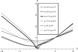
Figure 5: $a$ vs $T$ for $\sigma=1.0$, $a_{i}=1.0$, $T_{i}=1.0$ $\omega=\frac{1}{3}$.

The numerical solution of Eq. (59) also encompasses multiple bounces for certain values of the parameters $\sigma$, $p_{1}$ and $p_{2}$ and of the initial values $a_{i}$ and $T_{i}$. See figure 6.

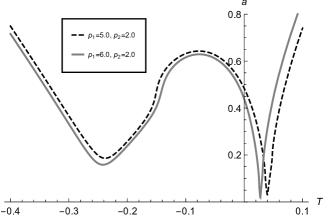
Figure 6: $a$ vs $T$ for $\sigma=1.5$, $a_{i}=5.0$, $T_{i}=1.0$, $\omega=\frac{1}{3}$.

As we did for the other bounce solutions, we express the wave function parameters in terms of cosmological quantities. Expanding the square of the correspondent Hubble function for large times $T$, we obtain

$$H^{2}=\frac{a_{i}^{2}}{a^{4}(T_{i}^{2}+\sigma^{4})}.$$ (61)

Identifying the dimensionless density parameter for radiation today $\Omega_{r0}=\rho_{r0}/\rho_{c0}$ as the coefficient of $(a_{0}/a)^{4}$, we obtain

$$\Omega_{r0}=\frac{a_{i}^{2}}{a_{0}^{4}H_{0}^{2}(T_{i}^{2}+\sigma^{4})}.$$ (62)

In order to rewrite Eq. (62) in terms of $a_{b}$ and $T_{b}$, we expand Eq. (59) for $T/\sigma^{2}\ll 1$ to the first order and for $p_{1}\sigma\ll 1$ and $p_{2}\sigma\ll 1$ to the second order. Under these conditions, i.e. near the bounce and with small parameters related to asymmetry, we obtain a solution with a single bounce, where it is possible to relate $T_{b}$, $p_{1}$ and $p_{2}$ by making $da/dT=0$. Disregarding also terms containing $p_{1}^{2}p_{2}^{2}$, we obtain

$$T_{b}=\frac{(p_{1}^{2}-p_{2}^{2})\sigma^{4}}{2}.$$ (63)

Performing the following transformation of variables

$$x_{b} = \frac{a_{0}}{a_{b}}$$ (64)

$$\overline{\sigma} = \sigma\sqrt{a_{0}H_{0}}$$ (65)

$$\overline{p}_{1}^{2} = \frac{p_{1}^{2}}{a_{0}H_{0}}$$ (66)

$$\overline{p}_{2}^{2} = \frac{p_{2}^{2}}{a_{0}H_{0}},$$ (67)

we obtain

$$\overline{\sigma}^{2}=\sqrt{\frac{2}{x_{b}^{2}\Omega_{r0}+\sqrt{x_{b}^{2}\Omega_{r0}[(\overline{p}_{1}^{2}-\overline{p}_{2}^{2})^{2}+x_{b}^{2}\Omega_{r0}]}}}.$$ (68)

Note that Eqs. (61, 62, 68) reduce to their correspondents in the symmetric case Eqs. (19, 20, 23) for $\overline{p}_{1}=\overline{p}_{2}=0$, which implies $T_{i}=T_{b}=0$.

For this particular case, i.e. $T/\sigma^{2}\ll 1$ to first order and for $p_{1}\sigma\ll 1$ and $p_{2}\sigma\ll 1$ to second order, the curvature scale at the bounce $L_{b}$ assumes the same form of the symmetric case given by Eq. (24), but with $\overline{\sigma}^{2}$ given by (68).

We now go back to the general case given by Eq. (59) and verify for which values of the parameters the bounce scale is larger than the Planck scale and smaller than the nucleosynthesis scale. We find $L_{b}$ numerically for some non-multiple asymmetric bounces, and we obtain the correspondent bounce energy $E_{b}=L_{b}^{-1/2}$ for each case. The results are shown in table 1.

$p_{1}\sigma$	$p_{2}\sigma$	$L_{b}$ (s)	$E_{b}$ (MeV)
$2.5$	$1.0$	$3.59934\times 10^{-3}$	$16.66820$
$3.5$	$1.0$	$5.95604\times 10^{-4}$	$40.97522$
$4.5$	$1.0$	$1.61263\times 10^{-4}$	$78.74681$
$5.5$	$1.0$	$5.75934\times 10^{-5}$	$131.76909$
$6.5$	$1.0$	$1.19055\times 10^{-5}$	$201.63933$
$7.5$	$1.0$	$4.78629\times 10^{-5}$	$289.81846$
$8.5$	$1.0$	$6.32385\times 10^{-6}$	$397.65741$
$9.5$	$1.0$	$3.60849\times 10^{-6}$	$526.42560$
$10.5$	$1.0$	$2.17979\times 10^{-6}$	$677.31783$
$1.0$	$2.5$	$5.64555\times 10^{-3}$	$13.30904$
$1.0$	$3.5$	$1.00531\times 10^{-3}$	$31.53917$
$1.0$	$4.5$	$2.75388\times 10^{-4}$	$60.25975$
$1.0$	$5.5$	$9.80995\times 10^{-5}$	$100.96402$

Table 1: $L_{b}$ and $E_{b}$ for $\sigma=1.0,a_{i}=1.0,T_{i}=1.0,\omega=\frac{1}{3}$.

Once $L_{p}\approx 5\times 10^{-44}\ s$, we see that $L_{b}>>L_{p}$ for all bounces considered. As mentioned before, this means that the validity of the Wheeler-DeWitt equation as an approximation to a more fundamental theory of gravity is well established. Beyond that, the bounce must occur at energy scales much larger than the nucleosynthesis scale, i.e. $10$MeV, which is not achieved by all cases considered. Indeed, as one can see from table I, the energy scale of such bounces are not much bigger than the nucleosynthesis energy scale, but they are many orders of magnitude smaller than the Planck energy scale. Hence, the physically relevant consistency check of such bouncing models is the upper limit of $L_{b}$, not its lower limit, which makes the distinction between $L_{b}$ and $L_{\rm min}$ irrelevant.

The cases $p_{1}\sigma\geqslant 10.9$, $p_{2}\sigma=1.0$ and $p_{1}\sigma=1.0$, $p_{2}\sigma\geqslant 5.8$ represent multiple bounces. Multiple bounces are also encountered in quantum reduced loop cosmology, in a scenario called emergent bounce LQC . It describes a series of bounces with successive increasing amplitudes. In our work, the multiple bounces do not necessarily present this behaviour. The solutions we found also allow for more than one bounce, but with similar amplitudes, before being launched to the expanding phase.

V Conclusion

We have obtained generalizations of the quantum bounce solutions obtained in Refs Pinto-Neto:2013toa ; PintoNeto:2004uf which are asymmetric with respect to the bounce, and even possessing multiple bounces. These solutions may be used to take into account significant back-reaction due to quantum particle production around the bounce, see Refs. Celani2017 ; Scardua2018 . As an example, in future work we will investigate baryogenesis in those asymmetric bounces.

One particular class of interesting solutions is the one exhibited in figure 4. It describes expanding cosmological solutions arising from an almost flat space-time. As discussed in Section III, the energy density at contraction can be made arbitrarily small, depending on the new quantum parameter $p$, related to the phase velocity of the initial wave function of the universe. The emerging picture is of an arbitrarily flat and almost empty space-time, which is launched through a bounce into the standard Friedmann expanding phase, containing the usual hot and dense radiation field. This fact open new windows to an old speculation, that our Universe arose from quantum fluctuations of a fundamental quantum vacuum. The de Broglie-Bohm theory allows a different regard to this hypothesis and the concrete possibility to extend this particular mini-superspace model by incorporating quantum cosmological perturbations to the system and quantitatively study their observational effects. This is also subject for future work.

- (1) S. W. Hawking and R. Penrose 1970 Royal Society 314 1519
- (2) H. Everett 1957 Rev. Mod. Phys. 29 454
- (3) G.C. Ghirardi, A. Rimini and T. Weber 1986 Phys. Rev. D 34 470; G.C. Ghirardi, P. Pearle and A. Rimini 1990 Phys. Rev. A 42 78
- (4) D. Bohm 1952 Phys. Rev. 85 166
- (5) D. Bohm 1952 Phys. Rev. 85 180
- (6) N. Pinto-Neto and J. C. Fabris 2013 Class. Quant. Grav. 30 143001
- (7) P. Peter and N. Pinto-Neto 2008 Phys. Rev. D 78 063506
- (8) P. Peter and S. D. P. Vitenti 2016 Mod. Phys. Lett. A 31 21 1640006
- (9) A. P. Bacalhau, P. Peter and S. D. P. Vitenti 2017 Phys. Rev. D 96 2 023517
- (10) R. L. Arnowitt, S. Deser and C. W. Misner 2008 Gen. Rel. Grav. 40 1997
- (11) B. F. Schutz 1970 Phys. Rev. D 2 2762
- (12) J. J. Halliwell 1988 Phys. Rev. D 38 2468
- (13) D. M. Gitman, I. V. Tyutin and B. L. Voronov 2012 Self-adjoint Extensions in Quantum Mechanics (Birkhäuser Basel, Boston).
- (14) D. Dürr, S. Goldstein and N. Zanghì 2004 Journal of Statistical Physics 116 959
- (15) F. T. Falciano and N. Pinto-Neto 2009 Phys. Rev. D 79 023507
- (16) C. Kiefer 2009 Gen. Rel. Grav. 41 877-90
- (17) E. Abraham, S. Colin and A. Valentini 2014 J. Phys. A: Math. Theor. 47 395306
- (18) S. D. P. Vitenti, P. Peter and A. Valentini 2019 Phys. Rev. D 100 043506
- (19) S. Gryb and K. P. Y. Thébault 2018 Phys. Lett. B 784 324
- (20) S. Gryb and K. P. Y. Thébault 2019 Class. Quant. Grav. 36 035009, 035010
- (21) E. Alesci, A. Barrau, G. Botta, K. Martineau and G. Stagno 2018 Phys. Rev. D 98 106022
- (22) D. C. F. Celani, N. Pinto-Neto and S. D. P. Vitenti 2017 Phys. Rev. D 95 24700029
- (23) A. Scardua, L. F. Guimarães and N. Pinto-Neto and G. S. Vicente 2018 Phys. Rev. D 98 083505
- (24) S. Gryb and K. P. Y. Thébault 2018 Phys. Lett. B 784 324
- (25) S. Gryb and K. P. Y. Thébault 2019 Class. Quant. Grav. 36 035009
- (26) E. Alesci, A. Barrau, G. Botta, K. Martineau and G. Stagno 2018 Phys. Rev. D 98 106022