Postural Stability in Human Running with Step-down Perturbations
An Experimental and Numerical Study

Abstract

Postural stability is one of the most crucial elements in bipedal locomotion. Bipeds are dynamically unstable and need to maintain their trunk upright against the rotations induced by the ground reaction forces (GRFs), especially when running. Gait studies report that the GRF vectors focus around a virtual point above the center of mass ($\mathrm{VP_{\color[rgb]{0.1294,0.4000,0.6745}{A}}}$), while the trunk moves forward in pitch axis during the stance phase of human running. However, a recent simulation study suggests that a virtual point below the center of mass ($\mathrm{VP_{\color[rgb]{0.6980,0.0941,0.1686}{B}}}$) might be present in human running, since a $\mathrm{VP_{\color[rgb]{0.1294,0.4000,0.6745}{A}}}$ yields backward trunk rotation during the stance phase. In this work, we perform a gait analysis to investigate the existence and location of the VP in human running at $5\text{\,}\mathrm{m}\text{\,}{\mathrm{s}}^{-1}$, and support our findings numerically using the spring-loaded inverted pendulum model with a trunk (TSLIP). We extend our analysis to include perturbations in terrain height (visible and camouflaged), and investigate the response of the VP mechanism to step-down perturbations both experimentally and numerically. Our experimental results show that the human running gait displays a $\mathrm{VP_{\color[rgb]{0.6980,0.0941,0.1686}{B}}}$ of $\approx\scalebox{0.65}[1.0]{$-$}30\text{\,}\mathrm{cm}$ and a forward trunk motion during the stance phase. The camouflaged step-down perturbations affect the location of the $\mathrm{VP_{\color[rgb]{0.6980,0.0941,0.1686}{B}}}$. Our simulation results suggest that the $\mathrm{VP_{\color[rgb]{0.6980,0.0941,0.1686}{B}}}$ is able to encounter the step-down perturbations and bring the system back to its initial equilibrium state.

1 Introduction

Bipedal locomotion in humans poses challenges for stabilizing the upright body due to the under-actuation of the trunk and the hybrid dynamics of the bipedal structure.

Human gait studies investigate the underlying mechanisms to achieve and maintain the postural stability in symmetrical gaits such as walking and running. One major observation states that the ground reaction forces (GRFs) intersect near a virtual point (VP) above the center of mass (CoM) [maus2010upright]. Subsequent gait studies report that the VP is $15\scalebox{0.65}[1.0]{$-$}50\text{\,}\mathrm{cm}$ above the CoM ($\mathrm{VP_{\color[rgb]{0.1294,0.4000,0.6745}{A}}}$) in sagittal plane for level walking [gruben2012force, maus2010upright, muller2017force, Sharbafi_2015a, vielemeyer2019ground]. Among those, only a single study reports a limited set of level walking trials with a VP below the CoM ($\mathrm{VP_{\color[rgb]{0.6980,0.0941,0.1686}{B}}}$) [maus2010upright]. The $\mathrm{VP_{\color[rgb]{0.1294,0.4000,0.6745}{A}}}$ strategy is also observed when coping with the step-down perturbations in human walking, even when walking down a camouflaged curb [vielemeyer2019ground]. A similar behavior is observed for the avians, where a $\mathrm{VP_{\color[rgb]{0.1294,0.4000,0.6745}{A}}}$ of $5\text{\,}\mathrm{cm}$ is reported for level walking, grounded running, and running of the quail [andrada2014trunk, blickhan2015positioning]. Unlike in the studies with healthy subjects, it is reported that humans with Parkinson’s disease display a $\mathrm{VP_{\color[rgb]{0.6980,0.0941,0.1686}{B}}}$ when walking [Scholl_2018]. In addition, a $\mathrm{VP_{\color[rgb]{0.6980,0.0941,0.1686}{B}}}$ was identified in the frontal plane for human level walking [Firouzi_2019]. The existing literature for human running report a $\mathrm{VP_{\color[rgb]{0.1294,0.4000,0.6745}{A}}}$ [blickhan2015positioning, Maus_1982]. However, these experiments are limited to a small subset of subjects and trials, hence are not conclusive.

The observation of the GRFs intersecting at a virtual point suggests that there is potentially a control mechanism to regulate the whole body angular momentum [maus2008stable, maus2010upright, Hinrichs_1987]. Based on this premise, the behavior of a VP based postural mechanism would depend of the location and adjustment of the VP. It also raises the question whether the VP position depends on the gait type, locomotor task (e.g., control intent) and terrain conditions.

The spring-mass model (SLIP) is extensively used in gait analysis due to its capability to reproduce the key features of bipedal locomotion. The SLIP model is able to reproduce the CoM dynamics observed in human walking [geyer2006compliant] and running [blickhan1989spring, McMahon_1990, Mueller_2016]. This model can be extended with a rigid body (TSLIP) to incorporate the inertial effects of an under-actuated trunk, where the trunk is stabilized through a torque applied at the hip [Maus_1982, maus2008stable, maus2010upright].

Based on the experimental observations, the VP is proposed as a control method to determine the hip torque in the TSLIP model to achieve postural stability [maus2008stable]. The VP as a control mechanism in TSLIP model is implemented for human walking [Lee_2017_I, Maufroy_2011, Sharbafi_2015a, Vu_2017_III, Vu_2017_II], hopping [Sharbafi_2012, Sharbafi_2013], running [maus2008stable, drama2019human, VanBommel_2011], and avian gaits [andrada2014trunk, drama2019bird]. It is also implemented and tested on the ATRIAS robot for a walking gait [Peekema_2015]. Yet the currently deployed robotic studies are limited to a small set of gait properties (e.g., forward speed) and simple level terrain conditions.

In the simulation model, the selection of the VP position influences the energetics of the system by distributing the work performed by the leg and the hip [drama2019human, drama2019bird]. A $\mathrm{VP_{\color[rgb]{0.6980,0.0941,0.1686}{B}}}$ in the human TSLIP model reduces the leg loading at the cost of increased peak hip torques for steady-state gaits. A $\mathrm{VP_{\color[rgb]{0.1294,0.4000,0.6745}{A}}}$ yields lower duty factors and hence higher peak vertical GRF magnitudes, whereas a $\mathrm{VP_{\color[rgb]{0.6980,0.0941,0.1686}{B}}}$ yields larger peak horizontal GRF magnitudes. Consequently, a $\mathrm{VP_{\color[rgb]{0.1294,0.4000,0.6745}{A}}}$ can be used to reduce the kinetic energy fluctuations of the CoM, and a $\mathrm{VP_{\color[rgb]{0.6980,0.0941,0.1686}{B}}}$ to reduce the potential energy fluctuations.

In human gait, the trunk moves forward during the single stance phase of walking and running, which is reversed by a backward trunk motion in double stance phase of walking [thorstensson1984trunk] and flight phase of running [Maus_1982, thorstensson1984trunk]. In TSLIP model simulations of human running, the trunk moves forward during the stance phase if a $\mathrm{VP_{\color[rgb]{0.6980,0.0941,0.1686}{B}}}$ is used, whereas it moves backward for a $\mathrm{VP_{\color[rgb]{0.1294,0.4000,0.6745}{A}}}$ [drama2019bird, drama2019human, maus2008stable, sharbafi2014stable].

One potential reason for the differences between the human and the model may be that the TSLIP model does not distinguish between the trunk and whole body dynamics. In human walking, the trunk pitching motion is reported to be $180\text{\,}\mathrm{\SIUnitSymbolDegree}$ out-of-phase with the whole body [gruben2012force]. A $\mathrm{VP_{\color[rgb]{0.1294,0.4000,0.6745}{A}}}$ in the TSLIP model predicts the whole body dynamics with backward rotation, and it follows that the trunk rotation is in the opposite direction (i.e., forward). The phase relation between the trunk and whole body rotation has not been published for human running, to our knowledge. However, we can indirectly deduce this relation from the pitch angular momentum patterns. In human running, the pitch angular momentum of the trunk and the whole body are inphase, and they both become negative during stance phase (i.e., clockwise rotation of the runner) [Hinrichs_1987]. The negative angular momentum indicates that the GRFs should pass below the CoM. Therefore, a $\mathrm{VP_{\color[rgb]{0.6980,0.0941,0.1686}{B}}}$ in the TSLIP model is able to predict the whole body dynamics with forward rotation, and the trunk rotation is in the same direction (i.e., forward).

The VP can also be used to maneuver, when the VP target is placed out of the trunk axis [maus2008stable, Sharbafi_2013]. A simulation study proposes to shift the VP position horizontally as a mechanism to handle stairs and slopes [Kenwright_2011]. The gait analyses provide insights into the responses of GRFs to changes in terrain. In human running, step-down perturbations increase the magnitude of the peak vertical GRF. The increase gets even higher if the drop is camouflaged [muller2012leg]. However, there is no formalism to describe how the VP position relates to the increase in GRFs in handing varying terrain conditions.

In the first part of our work, we perform an experimental analysis to acquire trunk motion patterns and ground reaction force characteristics during human running. Our gait analysis involves human level running, and running over visible and camouflaged step-down perturbations of $\scalebox{0.65}[1.0]{$-$}10\text{\,}\mathrm{cm}$. We expect to observe a net forward trunk pitch motion during the stance phase of running based on the observation in [thorstensson1984trunk], and estimate a $\mathrm{VP_{\color[rgb]{0.6980,0.0941,0.1686}{B}}}$ from the GRF data based on the hypothesis in [drama2019human].

In the second part, we perform a simulation analysis using the TSLIP model with the gait parameters estimated from our experiments. We generate an initial set of gaits that match to the experimental setup, and extend our analysis to larger set of step-down perturbations up to $\scalebox{0.65}[1.0]{$-$}40\text{\,}\mathrm{cm}$, which is close to the maximum achievable perturbation magnitude in avians [BirnJeffery_2014]. We investigate whether a $\mathrm{VP_{\color[rgb]{0.6980,0.0941,0.1686}{B}}}$ controller is able to stabilize the gait against the step-down perturbations, and if so, how does it contribute to the energy flow in counteracting the perturbation.

2 Methods

2.1 Experimental Methods

In this section, we describe the experimental setup and measurement methods. In our experiments, ten physically active volunteers (9 male, 1 female, mean $\pm$ s.d., age: $24.1\pm 3.4$ years, mass: $73.8\pm 7.3\text{\,}\mathrm{kg}$, height: $179.9\pm 7.6\text{\,}\mathrm{cm}$) are instructed to run over a $17\text{\,}\mathrm{m}$ track. The running track has two consecutive force plates in its center, where the first plate is fixed at ground-level, and the second one is height adjustable. We designed three sets of experiments, where the subjects were asked to run at their self-selected velocity ($4.9\pm 0.5\text{\,}\mathrm{m}\text{\,}{\mathrm{s}}^{-1}$, table 1). In the first experiment, the subjects were asked to run on a track with an even ground (V0). In the second experiment, the second force plate was lowered $\scalebox{0.65}[1.0]{$-$}10\text{\,}\mathrm{cm}$, which was visible to the subjects (V10). In the third experiment, the second force plate was lowered $\scalebox{0.65}[1.0]{$-$}10\text{\,}\mathrm{cm}$, and an opaque sheet was added on top of the plate on ground level to camouflage the drop. A wooden block was randomly placed between the second force plate and the opaque sheet during the course of the experiment without subject’s knowledge. In other words, the subjects were not aware whether the step would be on the ground level (C0), or would be a step-down drop (C10). The step corresponding onto the first force plate is referred to as step -1, and the step to the second force plate as step 0.

Figure 1: Experimental setup. The first force plate is on the ground level, whereas the second force plate is height adjustable (step 0). The camouflaged setting for the second force plate is shown on right for elevations of $0\text{\,}\mathrm{cm}$ (C0, blue) and $-10\text{\,}\mathrm{cm}$ (C10, red). The placement of the motion capture markers is given on left, where the markers are denoted the letters A-G. The trunk angle is shown with $\gamma$ and is positive in the counterclockwise direction.

All trials were recorded with eight cameras by a 3D motion capture system working with infrared light. In sum twelve spherical reflective joint markers (19 mm diameter) were placed on the tip of the fifth toe [A], malleolus lateralis [B], epicondylus lateralis femoris [C], trochanter major [D], and acromion [E] on both sides of the body as well as on L5 [F] and C7 [G] processus spinosus (see figure 1). The CoM was determined with a body segment parameter method according to winter2009biomechanics. The trunk angle $\gamma$ was calculated from the line joining C7 to L5 with respect to the vertical [muller2014kinetic].

Further information concerning the participants, and the technical details of the measurement equipment (i.e., force plates, cameras) can be found in muller2012leg and partly in ernst2014vertical.

The method for analyzing the gait data and estimating a potential VP is analogous to the gait analysis carried out for the human walking in [vielemeyer2019ground]. Here, we denote the intersection point of the GRF vectors as a VP without implications for this point being above or below the CoM. To compute the VP, we use the instantaneous GRF vectors, which have an origin at the center of pressure (CoP) and are expressed in a CoM-centered coordinate frame that aligns with the gravity vector in vertical axis [muller2017force]. The CoP is calculated from the kinetic data using the method described in winter2009biomechanics. Then, the VP is estimated as the point, which minimizes the sum of the squared distances between the GRF vectors and itself. For the camouflaged setting with a wooden block placed on the force plate (C0), we can not calculate the CoP accurately. Thus, the VP is not estimated for C0 case.

The human gait data involves impact forces at the leg touch-down, which introduces an additional behavior in the GRF pattern [muller2012leg, gunther2003dealing, vanderLinden2009hitting]. In order to see the influence of the impact on VP, we are presenting our recorded data in two ways. First calculation involves the full GRF data from leg touch-down to take-off ($100\text{\,}\mathrm{\char 37\relax}$ dataset), whereas the second calculation involves the GRF data starting from $10\text{\,}\mathrm{\char 37\relax}$ of the stance to the leg take-off ($90\text{\,}\mathrm{\char 37\relax}$ dataset).

In theory of VP, all of the GRF vectors start from the CoP and point to a single virtual point. However, the human gait data differs from this theoretical case, as the human is more complex. To evaluate the amount of agreement between the theoretical VP based forces and experimentally measured GRFs, we use a measure called the coefficient of determination ($R^{2}$) similar to herr2008angular:

$$R^{2}\;=\;\left(1\;-\;\frac{{{\sum\limits}}_{i=1}^{N_{trial}}{{\sum}}\limits_{j=1}^{N_{\%}}\left(\theta^{ij}_{exp}-\theta^{ij}_{theo}\right)^{2}}{{{\sum}}\limits_{i=1}^{N_{trial}}{{\sum}}\limits_{j=1}^{N_{\%}}\left(\theta^{ij}_{exp}-\overline{\theta}_{exp}\right)^{2}}\right)\times 100\%,$$ (1)

The ($\theta_{exp}$, $\theta_{theo}$) are the experimental GRF and theoretical force vector angles, $N_{trial}$ is the number of trials, and $N_{\%}=100$ is the measurement time. Here, $\overline{\theta}_{exp}$ is the mean of the experimental GRF angles over all trials and measurement times. The number of trials is equal to 30 for visible conditions (15 for V0 and 15 for V10) and 20 for the camouflaged conditions (12 for C0 and 8 for C10).

Note that $R^{2}=$100\text{\,}\mathrm{\char 37\relax}$$ if there is a perfect fit for the experimental GRF and the theoretical force vector angles. The value of $R^{2}$ aproaches zero as the estimation of the model is equal to the use of ${\theta}_{exp}$ as an estimator [herr2008angular].

We also compute the horizontal and vertical impulses $\vec{p}$ for two intervals (braking and propulsion) by integrating the GRFs over time. The braking interval went from touch-down to mid-stance (zero-crossing of the horizontal GRFs) and the propulsion interval mid-stance onward. We report the values for brake-propulsion intervals individually in Section 3.1. To enable the comparison among subjects, we normalize the impulses to each subject’s body weight ($\mathrm{BW}$), leg length ($l$, the distance between lateral malleolus and trochanter major of the leg in contact with the ground) and standard gravity ($g$) in accordance with [hof1996scaling] as,

$$\vec{p}_{normalized}\;=\;\frac{\vec{p}}{\mathrm{BW}\cdot\sqrt{l/g}}.$$ (2)

Because of the inaccuracy in calculating the CoP, we did not analyze the C0 statistically. For all other experimental settings (V0, V10, and C10), we used repeated measures ANOVA ($p<0.05$) with post hoc analysis (Šidák correction) to test the statistical significance of the estimated VP position, the impulses and additional gait properties. In order to verify whether the VP is above or below the CoM ($\mathrm{VP_{\color[rgb]{0.1294,0.4000,0.6745}{A}}}$ or $\mathrm{VP_{\color[rgb]{0.6980,0.0941,0.1686}{B}}}$), we performed a one-sample t-test compared with zero, separately for each condition with Šidák correction.

2.2 Simulation Methods

In this section, we describe the TSLIP model that we use to analyze how the VP reacts to the step-down perturbations in human running. The TSLIP model consists of a trunk with mass $m$ and moment of inertia $J$, which is attached to a massless leg of length $l$ and a massless point foot $F$ (see figure 2a). The leg is passively compliant with a parallel spring-damper mechanism, whereas the hip is actuated with a torque ${\tau}_{H}$. The dynamics of the system is hybrid, which involves a flight phase that has ballistic motion, followed by a stance phase that reflects the dynamics of the spring-damper-hip mechanism. The phases switch when the foot becomes in contact with the ground at touch-down, and when the leg extends to its rest length $l_{0}$ at take-off.

The equations of motion for the CoM state $(x_{C},z_{C},\theta_{C})$ during the stance phase can be written as in equation 3, where the linear leg spring force $F_{sp}\mkern 1.5mu{=}\mkern 1.5muk\,(l\scalebox{0.65}[1.0]{$-$}l_{0})$ and bilinear leg damping force $F_{dp}\mkern 1.5mu{=}\mkern 1.5muc\,\dot{l}\,(l\scalebox{0.65}[1.0]{$-$}l_{0})$ generate the axial component of the GRF in foot frame $\prescript{}{F}{\mathbf{F}}_{a}\mkern 1.5mu{=}\mkern 1.5mu\left(F_{sp}\scalebox{0.65}[1.0]{$-$}F_{dp}\right){\left[\scalebox{0.65}[1.0]{$-$}\cos\theta_{L}\;\sin\theta_{L}\right]}^{\mathsf{T}}$. Here, $k$ refers to the spring stiffness and $c$ to the damping coefficient.  The hip torque ${\tau}_{H}$ creates the tangential component of the GRF $\prescript{}{F}{\mathbf{F}}_{t}\mkern 1.5mu{=}\mkern 1.5mu\left(\mathchoice{\raisebox{-3.5251pt}{\leavevmode\resizebox{9.27118pt}{12.0pt}{\hbox{\raisebox{4.42888pt}{$\displaystyle\frac{\scalebox{0.65}[1.0]{$-$}\tau_{H}}{l_{L}}$}}}}}{\raisebox{-3.52238pt}{\leavevmode\resizebox{9.30598pt}{12.0pt}{\hbox{\raisebox{3.11388pt}{$\textstyle\frac{\scalebox{0.65}[1.0]{$-$}\tau_{H}}{l_{L}}$}}}}}{\raisebox{-3.47357pt}{\leavevmode\resizebox{9.93369pt}{12.0pt}{\hbox{\raisebox{2.41943pt}{$\scriptstyle\frac{\scalebox{0.65}[1.0]{$-$}\tau_{H}}{l_{L}}$}}}}}{\raisebox{-3.47357pt}{\leavevmode\resizebox{9.93369pt}{12.0pt}{\hbox{\raisebox{2.41943pt}{$\scriptscriptstyle\frac{\scalebox{0.65}[1.0]{$-$}\tau_{H}}{l_{L}}$}}}}}\right){\left[\sin\theta_{L}\;\scalebox{0.65}[1.0]{$-$}\cos\theta_{L}\right]}^{\mathsf{T}},$ (see figure 2d).

$$m\begin{bmatrix}\ddot{x}_{C}\\ \ddot{z}_{C}\end{bmatrix} \mkern 1.5mu{=}\mkern 1.5mu\prescript{}{F}{\mathbf{F}}_{a}+\prescript{}{F}{\mathbf{F}}_{t}+g,$$ (3)

$$\vspace{0.5cm}J\,\ddot{\theta}_{C} \mkern 1.5mu{=}\mkern 1.5mu\scalebox{0.65}[1.0]{$-$}{\mathbf{r}}_{FC}\mkern 1.5mu{\times}\mkern 1.5mu(\prescript{}{F}{\mathbf{F}}_{a}+\prescript{}{F}{\mathbf{F}}_{t}).$$

Figure 2: a) TSLIP model that shows the forward (anterior) and backward (posterior) trunk motion. b) Vector notations used in equations of motion. c) The parameter space for the VP is divided into two regions: the virtual points above the center of mass ($\mathrm{VP_{\color[rgb]{0.1294,0.4000,0.6745}{A}}}$) and below ($\mathrm{VP_{\color[rgb]{0.6980,0.0941,0.1686}{B}}}$). $\mathrm{VP_{\color[rgb]{0.1294,0.4000,0.6745}{A}}}$ causes backward and $\mathrm{VP_{\color[rgb]{0.6980,0.0941,0.1686}{B}}}$ causes forward trunk rotation during the stance phase. Each subspace is divided further with respect to the leg axis, where the sign of the hip torque changes. d) For $\mathrm{VP_{\color[rgb]{0.6980,0.0941,0.1686}{B}}}$, the points above the leg axis yield a negative and points below ($\mathrm{VP_{\color[rgb]{0.3017,0.0004,0.0026}{BL}}}$) yield positive hip torque at touch-down. The VP is described with the radius ($r_{VP}$) and angle ($\theta_{VP}$) that is expressed in CoM centered world coordinate frame. Here presented human running experiments reveal that the VP is $\scalebox{0.65}[1.0]{$-$}30\text{\,}\mathrm{cm}$ below the CoM (see Section 3.1). This corresponds to the $\mathrm{VP_{\color[rgb]{0.3017,0.0004,0.0026}{BL}}}$ region with -$180\text{\,}\mathrm{\SIUnitSymbolDegree}$ VP angle in our simulation.

The leg and the hip maintain the energy balance of the system. The hip increases the system energy to propel the body forward, whereas the leg damper removes an equivalent energy in return. We determine $\tau_{H}$, such that the GRF points to a virtual point (VP), which is characterized by the radius $r_{VP}$ (i.e., distance between the hip and CoM) and angle $\theta_{VP}$, as shown in figure 2d ( ). The hip torque as a function of the VP is written as,

$$\tau_{H} =\tau_{VP}=\prescript{}{F}{\mathbf{F}}_{a}\times\left[\frac{\mathbf{r}_{FV}\times\mathbf{r}_{FH}}{\mathbf{r}_{FV}\cdot\mathbf{r}_{FH}}\right]\times l,$$ (4)

$$\vspace{0.5cm}\mathbf{r}_{FV} =\mathbf{r}_{FC}+r_{VP}\begin{bmatrix}[r]\scalebox{0.65}[1.0]{$-$}\sin\left(\theta_{C}+\theta_{VP}\right)\\ \cos\left(\theta_{C}+\theta_{VP}\right)\end{bmatrix}.$$

We utilize two linear controllers: one for the leg angle at touch-down $\theta_{L}^{TD}$, and other for the VP angle $\theta_{VP}$, both of which are executed at the beginning of the step at apex, as shown in figure LABEL:fig:Flowchart. The leg angle is regulated as,

with $\Delta\dot{x}|_{\text{-}1}^{i}$ being the difference in apex velocity $\dot{x}$ between time steps -$1$ and $i$. The VP angle is defined with respect to a CoM-centered, stationary coordinate frame that is aligned with the global vertical axis, if the VP is set below the CoM (see figures 2b, 2d) [drama2019bird]. It is adjusted based on the difference between the desired mean body angle $\theta_{C}^{Des}$, and the mean body angle observed in the last step $\Delta\theta_{C}$ as,

$$\theta_{VP}\ |_{i}=\theta_{VP}\ |_{i-1}+k_{vp}\left(\theta_{C}^{Des}\scalebox{0.65}[1.0]{$-$}\Delta\theta_{C}\right).$$ (6)

The model parameters are selected to match a $80\text{\,}\mathrm{kg}$ human with $1\text{\,}\mathrm{m}$ leg length (see table LABEL:tab:ModelPrm for details). The damping coefficient is set to $c\mkern 1.5mu{=}\mkern 1.5mu$$680\text{\,}\mathrm{kN}\text{\,}\mathrm{s}\text{\,}{\mathrm{m}}^{-1}$ to match the trunk angular excursion of $4.5\text{\,}\mathrm{\SIUnitSymbolDegree}$ reported in [Heitcamp_2012, Schache_1999, thorstensson1984trunk]. The forward speed and VP radius are set to $5\text{\,}\mathrm{m}\text{\,}{\mathrm{s}}^{-1}$ and $\scalebox{0.65}[1.0]{$-$}30\text{\,}\mathrm{cm}$ respectively, to match our estimated gait data in table 1. A VP radius of $\scalebox{0.65}[1.0]{$-$}30\text{\,}\mathrm{cm}$ becomes below the leg axis at leg touch-down with the model parameters we chose. Since the position of VP relative to the leg axis affects the sign of the hip torque, the $\mathrm{VP_{\color[rgb]{0.6980,0.0941,0.1686}{B}}}$ region is separated into two and the points below the leg axis are called $\mathrm{VP_{\color[rgb]{0.3017,0.0004,0.0026}{BL}}}$ (figure 2c- 2d), in accordance with [drama2019human].

First, we generate a base gait for level running using the framework in [drama2019human], which corresponds to the V0 in our human running experiments. Then, we introduce step-down perturbations of $\Delta z\mkern 1.5mu{=}\mkern 1.5mu$[$\scalebox{0.65}[1.0]{$-$}10,\scalebox{0.65}[1.0]{$-$}20,\scalebox{0.65}[1.0]{$-$}30,\scalebox{0.65}[1.0]{$-$}40\text{\,}\mathrm{cm}$] in step 0. The $\scalebox{0.65}[1.0]{$-$}10\text{\,}\mathrm{cm}$ drop corresponds to the V10 and C10 of the human running experiments. In the simulations, the VP controller is blind to the changes in step 0, since the controller update happens only at the apex of each step. The postural correction starts at step 1. In other words, we see the natural response of the system at step 0, and counteracting response of the VP controller starting from step 1. In contrast, there might already be a postural control during the step 0 in the experiments.

The step-down perturbation increases the total energy of the system. The added energy can be either dissipated e.g., via the hip torque or leg damper, or converted to other forms of energy e.g., change in speed or hopping height. In the latter case, we need to update the desired forward speed in the leg angle control (equation 5) until all excess energy is converted to kinetic energy.

We implemented the TSLIP model in Matlab using variable step solver ode113 with a relative and absolute integrator error tolerance of $1\times 10^{\scalebox{0.65}[1.0]{$-$}12}$.

3 Results

3.1 Experimental Results

The results and statistical values of the experiments are listed in table 1 and illustrated in figures 4 to 5, and connected with simulation results, in figures 6 to 11. Additionally, significant mean differences will be highlighted in the following.

[] []

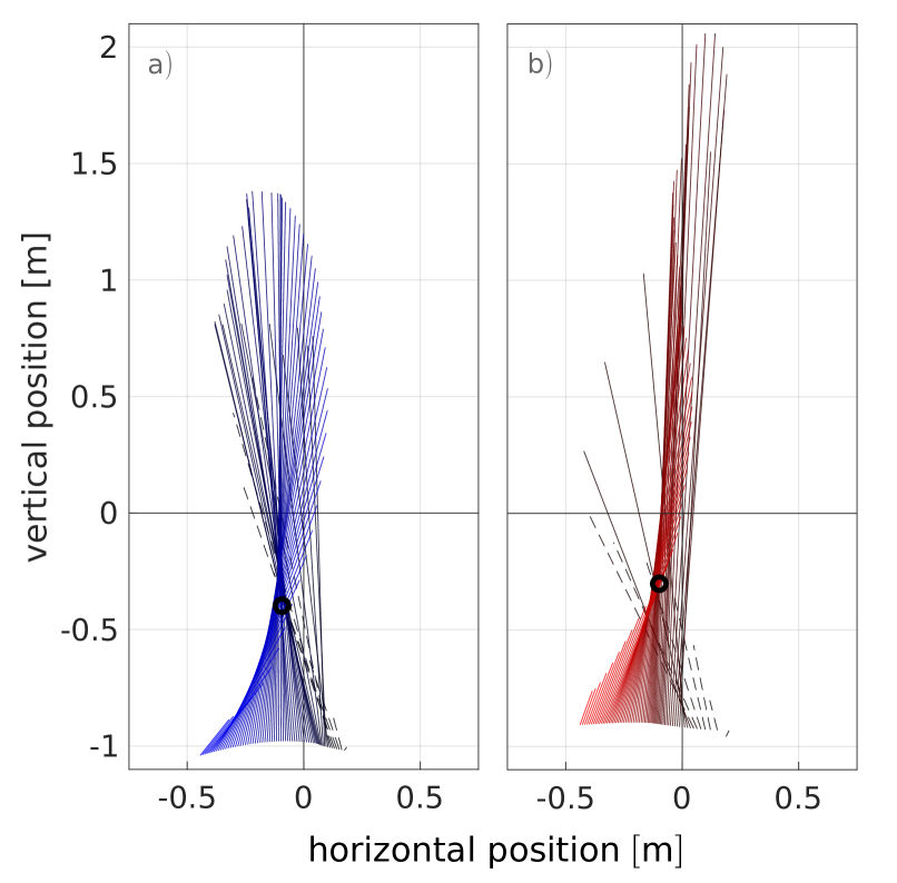
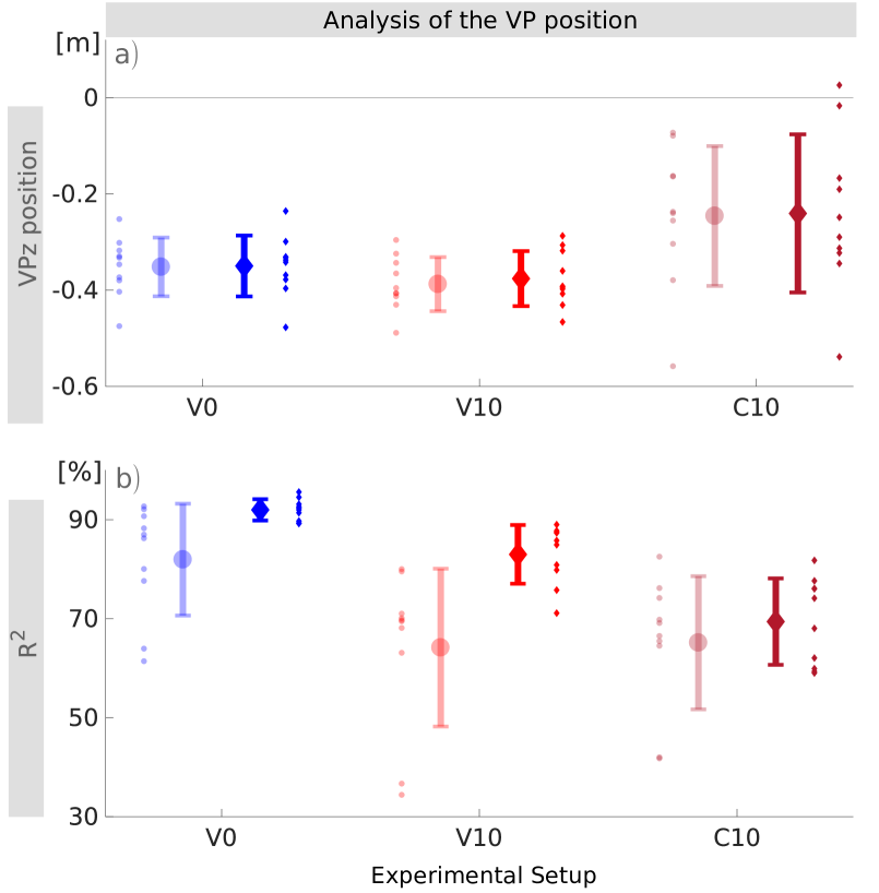
Figure 3: Examples of the ground reaction force vectors (GRFs) and the estimated virtual point (VP) for step 0 of V0 (a) and C10 (b) conditions of the human running experiments. The GRFs and VP are plotted with respect to a CoM-centered, stationary coordinate frame. Lines show the GRFs at different measurement times, originating at the CoP. The 90% dataset consists only of GRF data plotted as solid lines, the 100% dataset includes the entire stance phase GRF data. The black circle indicates the calculated VP for the $90\text{\,}\mathrm{\char 37\relax}$ dataset. a) V0: Visible level running, black to blue, b) C10: Running with a camouflaged drop of $-10\text{\,}\mathrm{cm}$, black to red. For each condition, the trial with the spread around the VP nearest to the 50^th percentile of all subjects was chosen.

Figure 4: Mean$\pm$s.d. of the vertical virtual point position VPz (a), and $R^{2}$ values (b) between subjects (N=10) for each ground condition (V0, V10 and C10) for step 0. a) Each small dot is the median over all trials of one condition for one subject. b) $R^{2}$ represents the ratio of the angle between measured and ideal forces and their variance. Each small dot represents one subject. Transparent circle: $100\text{\,}\mathrm{\char 37\relax}$ dataset, non-transparent diamond: $90\text{\,}\mathrm{\char 37\relax}$ dataset.

In figure 4, exemplary illustrations of the VP for single trials (V0 and C10) of different subjects at step 0 are shown. Here, the GRF vectors are plotted in a CoM-centered coordinate frame were the vertical axis is parallel to gravity. The VP is calculated as the point which minimizes the sum of squared perpendicular distances to the GRFs for each measurement time point. To avoid biases caused by the impact peak, the VP was additionally calculated for only $90\text{\,}\mathrm{\char 37\relax}$ of the dataset. That means that the GRFs of the first $10\text{\,}\mathrm{\char 37\relax}$ of the stance phase (dashed lines) were neglected in this VP calculation (figure 4). Hence, the VP was computed for $90\text{\,}\mathrm{\char 37\relax}$ and $100\text{\,}\mathrm{\char 37\relax}$ dataset and the results for both VP are given in this section.

The VP was in step -1 (pre-perturbed) and step 0 (perturbed) below the CoM (p<0.001) and between $\scalebox{0.65}[1.0]{$-$}38.8$ $\pm$ $5.6\text{\,}\mathrm{cm}$ and $\scalebox{0.65}[1.0]{$-$}24.0$ $\pm$ $16.4\text{\,}\mathrm{cm}$ (figure 4a). For step -1, there were no differences between the ground conditions in the vertical VP position VPz ($-31.0\text{\,}\mathrm{cm}$) and the $R^{2}$ ($88.7\text{\,}\mathrm{\char 37\relax}$; table 1). However, the horizontal VP position VPx was $5.5\text{\,}\mathrm{cm}$ (V10) and $5.7\text{\,}\mathrm{cm}$ (C10) more posterior in the drop conditions than in the level condition (p<0.001). At step 0, VPx was $4.4\text{\,}\mathrm{cm}$ more posterior in C10 compared to V0 (p<0.028) and for the 100% dataset $0.8\text{\,}\mathrm{cm}$ more posterior in V10 than in V0 (p=0.038; table 1). There were only differences in VPz for the 100% dataset, it was $3.6\text{\,}\mathrm{cm}$ lower in V10 compared to V0 (p=0.029). $R^{2}$ has the largest value for V0 (92.0 $\pm$ 2.1%; 90% dataset) and the smallest one for C10 (64.1 $\pm$ 8.7%; 100% dataset, figure 4b).

Table 1: Statistical analysis of VP, $R^{2}$, impulse and gait properties. V0, visible level running; V10 visible drop of $-10\text{\,}\mathrm{cm}$; C10, camouflaged drop of $-10\text{\,}\mathrm{cm}$; VP, horizontal (x) and vertical (z) positions of the virtual point relative to the center of mass for the 90% and the 100% dataset; $R^{2}$, coefficient of determination of the angles between measured ground reaction forces and forces through center of pressure and VP; $\vec{p}_{\mathrm{brake}}$, braking impulse and $\vec{p}_{\mathrm{prop}}$, propulsion impulse in the x- and z-direction. Data are means $\pm$ s.d. across all included subjects (N=10; exception: duty factor is only calculated for 9 subjects) for step -1 (pre-perturbed contact) and step 0 (perturbed contact). Post hoc analysis with Šidák correction revealed significant differences between ground conditions: differences from V0 and V10 are indicated with ’a’ and ’b’, respectively $(P<0.05)$.

		V0		V10		C10		p-value	F-Value/$\eta^{2}$
Step -1	VP variables
	$\mathrm{VPx_{100\%}}$ [$\centi\text{\,}\mathrm{]}$	-2.9$\pm$	2.9	-8.5$\pm$	3.5a	-8.6$\pm$	3.1a	0.000	224.38/0.01
	$\mathrm{VPx_{90\%}}$ [$\centi\text{\,}\mathrm{]}$	-3.4$\pm$	2.8	-8.7$\pm$	3.4a	-9.1$\pm$	3.2a	0.000	146.41/0.01
	$\mathrm{VPz_{100\%}}$ [$\centi\text{\,}\mathrm{]}$	-31.5$\pm$	4.9	-31.3$\pm$	5.0	-31.7$\pm$	6.6	0.965	0.04/0.00
	$\mathrm{VPz_{90\%}}$ [$\centi\text{\,}\mathrm{]}$	-30.8$\pm$	5.8	-30.7$\pm$	5.2	-31.5$\pm$	6.5	0.997	0.23/0.00
	$R_{\mathrm{100\%}}^{2}$ [$\text{\,}\!$]	76.0$\pm$	14.6	79.0$\pm$	12.1	77.3$\pm$	13.2	0.424	0.90/0.00
	$R_{\mathrm{90\%}}^{2}$ [$\text{\,}\!$]	88.1$\pm$	3.4	89.4$\pm$	3.4	88.5$\pm$	3.1	0.411	1.45/0.00
	Impulse
	$\vec{p}_{\mathrm{brake,x}}$	-0.05$\pm$	0.02	-0.05$\pm$	0.02	-0.04$\pm$	0.02	0.162	2.02/0.00
	$\vec{p}_{\mathrm{brake,z}}$	0.53$\pm$	0.11	0.47$\pm$	0.10	0.49$\pm$	0.06	0.051	3.53/0.01
	$\vec{p}_{\mathrm{prop,x}}$	0.11$\pm$	0.01	0.12$\pm$	0.02	0.11$\pm$	0.01	0.078	2.94/0.00
	$\vec{p}_{\mathrm{prop,z}}$	0.56$\pm$	0.02	0.57$\pm$	0.04	0.55$\pm$	0.04	0.421	0.91/0.00
Step 0	VP variables
	$\mathrm{VPx_{100\%}}$ [$\centi\text{\,}\mathrm{]}$	-2.8$\pm$	4.5	-4.0$\pm$	4.6a	-7.1$\pm$	5.1a	0.014	7.95/0.01
	$\mathrm{VPx_{90\%}}$ [$\centi\text{\,}\mathrm{]}$	-2.6$\pm$	4.6	-4.3$\pm$	4.7	-7.0$\pm$	5.0a	0.018	7.17/0.01
	$\mathrm{VPz_{100\%}}$ [$\centi\text{\,}\mathrm{]}$	-35.2$\pm$	6.1	-38.8$\pm$	5.6a	-24.6$\pm$	14.5	0.047	5.17/0.10
	$\mathrm{VPz_{90\%}}$ [$\centi\text{\,}\mathrm{]}$	-35.0$\pm$	6.3	-37.6$\pm$	5.7	-24.0$\pm$	16.4	0.074	4.04/0.10
	$R_{\mathrm{100\%}}^{2}$ [$\text{\,}\!$]	81.9$\pm$	11.3	64.1$\pm$	15.9a	65.1$\pm$	13.4	0.021	6.87/0.17
	$R_{\mathrm{90\%}}^{2}$ [$\text{\,}\!$]	92.0$\pm$	2.1	83.0$\pm$	5.9a	69.4$\pm$	8.7a,b	0.000	70.13/0.13
	Impulse
	$\vec{p}_{\mathrm{brake,x}}$	-0.10$\pm$	0.02	-0.11$\pm$	0.03	-0.04$\pm$	0.02a,b	0.000	40.27/0.01
	$\vec{p}_{\mathrm{brake,z}}$	0.69$\pm$	0.08	0.83$\pm$	0.12a	0.63$\pm$	0.12b	0.000	20.92/0.10
	$\vec{p}_{\mathrm{prop,x}}$	0.09$\pm$	0.02	0.09$\pm$	0.01	0.06$\pm$	0.01a,b	0.000	14.26/0.00
	$\vec{p}_{\mathrm{prop,z}}$	0.46$\pm$	0.08	0.48$\pm$	0.05	0.45$\pm$	0.06	0.309	1.19/0.01
	Gait properties
	velocity [$\text{\,}\mathrm{m}\text{\,}{\mathrm{s}}^{-1}$]	4.9$\pm$	0.5	4.9$\pm$	0.5	5.1$\pm$	0.4	0.148	2.13/0.11
	stance time [$\text{\,}\mathrm{]}$	0.18$\pm$	0.02	0.17$\pm$	0.02a	0.14$\pm$	0.01a,b	0.000	62.67/0.00
	duty factor [$\text{\,}\!$]	26.7$\pm$	2.0	24.8$\pm$	1.6a	22.4$\pm$	1.5a,b	0.008	37.20/0.01

There were no significant differences between the ground conditions in the impulses of step -1 (table 1). For step 0, figure 5 suggests that the vertical GRFs are higher in the step conditions compared to V0, especially for the braking phase. The vertical braking impulse was higher in V10 than in V0 (p=0.008) and in C10 (p<0.001). We observe $2.9\text{\,}\mathrm{BW}$ peak vertical GRFs in V0, which yield to a vertical braking impulse of 0.69. In V10, the peak vertical GRFs were at $3.4\text{\,}\mathrm{BW}$ with a braking impulse of 0.83. In C10, the peak was the highest with $3.9\text{\,}\mathrm{BW}$, but here, the peak is overlapping with the impact peak and therefore not comparable with that of the visible ground conditions (figure 5). Because of the shorter stance time in C10 (table 1), the braking impulse of 0.63 does not differ from the value of V0 despite the high impact peak. The vertical propulsion impulse of step 0 does not differ significantly between the ground conditions. The amounts of the horizontal braking and propulsion impulses were lower in C10 than in the visible conditions (p$\leq$0.004). The sum of the horizontal braking and propulsion impulses of step 0 is in all ground conditions around zero. That means that there is no forward acceleration or deceleration.

The vertical CoM position relative to the CoP at the touch-down of step 0 is $3.5\text{\,}\mathrm{cm}$ higher in the drop conditions compared to V0 (p<0.001) with $104.9\pm 5.2\text{\,}\mathrm{cm}$ and $1\text{\,}\mathrm{cm}$ higher in C10 than in V10 (p=0.019).

The forward running velocity measured at step 0 does not vary between the experiments V0, V10 and C10, and is within the range of $5.0\pm 0.5\text{\,}\mathrm{m}\text{\,}{\mathrm{s}}^{-1}$. Despite the constant velocity, the stance time and the duty factor of step 0 show a variation for between these experiments. The stance time gets shorter (p=0.029) and the duty factor lower (p<0.001) when running down the visible drop and even shorter and lower when the drop is camouflaged (p<0.006).

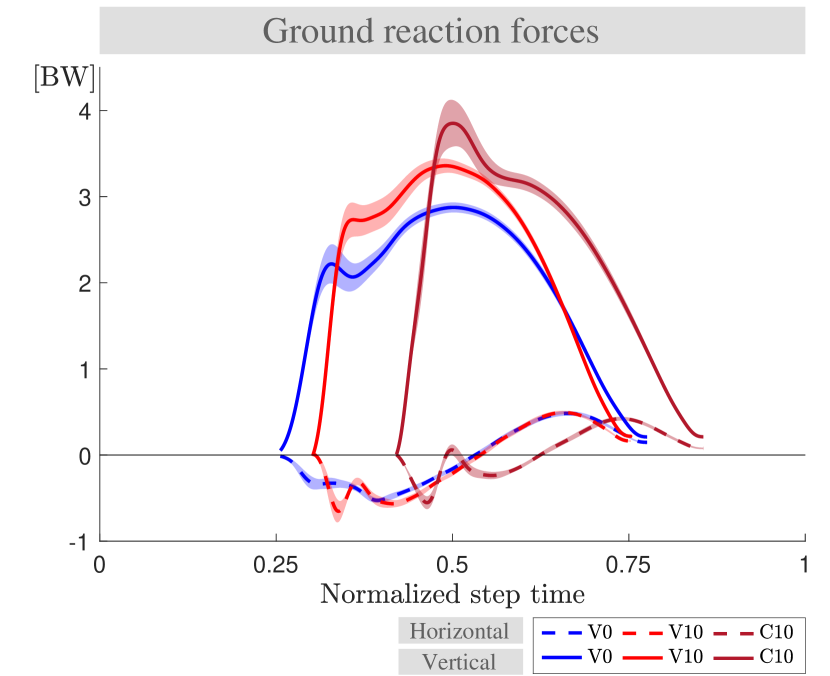
Figure 5: The ground reaction forces (GRFs) of step 0 for human running experiments V0 (blue), V10 (red), and C10 (brown). The GRF are normalized to body weight of the subjects (N=10) . The mean values of the vertical and horizontal GRF are plotted with solid and dashed lines, respectively. The $\pm$ standard error is shown with the shaded area. For the C10 condition, the vertical GRF peak coincides with the peak caused by the impact peak forces. The duty factor of the V0 condition is $26.7\pm 2.0\text{\,}\mathrm{\char 37\relax}$, whereas it is $24.8\pm 1.6\text{\,}\mathrm{\char 37\relax}$ for the V10 condition and $22.4\pm 1.5\text{\,}\mathrm{\char 37\relax}$ for the C10 condition.

3.2 Simulation Results

In this section, we present our simulation results and our analysis on how VP reacts to step-down perturbations. The simulation gaits are generated for $5\text{\,}\mathrm{m}\text{\,}{\mathrm{s}}^{-1}$ running with a VP target $\scalebox{0.65}[1.0]{$-$}30\text{\,}\mathrm{cm}$ below the CoM ($\mathrm{VP_{\color[rgb]{0.3017,0.0004,0.0026}{BL}}}$), which correspond to the estimated values of our experiments in Section 3.1.

The temporal properties of the base gait for the level running are given in table 2, where the duty factor is calculated as $26.2\text{\,}\mathrm{\char 37\relax}$ with a stance phase duration of $0.16\text{\,}\mathrm{s}$. The CoM trajectory of the base gait is shown in figure 3$a_{0}$ and its respective GRF vectors are plotted with respect to a hip centered stationary coordinate frame in figure 3$b_{0}$.

Table 2: Gait properties of the simulated trajectories. In the presence of step-down perturbations, the $\mathrm{VP_{\color[rgb]{0.3017,0.0004,0.0026}{BL}}}$ method is able to bring the system back to its initial equilibrium state. Therefore, the gait properties are the same for the even ground and perturbed terrain, after reaching to the steady state condition

.

Property Unit Value Property Unit Value Duty factor [$\%$] 26.2 VP angle [$\mathrm{\SIUnitSymbolDegree}$] -180 Stance time [s] 0.16 Trunk angular excursion [$\mathrm{\SIUnitSymbolDegree}$] 4.45 Forward speed [$\mathrm{m}\text{\,}{\mathrm{s}}^{-1}$] 5 Leg angle at touch-down [$\mathrm{\SIUnitSymbolDegree}$] 66

The base gait is subjected to step-down perturbations of $\Delta z\mkern 1.5mu{=}\mkern 1.5mu$[$\scalebox{0.65}[1.0]{$-$}10,\scalebox{0.65}[1.0]{$-$}20,\scalebox{0.65}[1.0]{$-$}30,\scalebox{0.65}[1.0]{$-$}40\text{\,}\mathrm{cm}$] at step 0. The VP controller updates on step-to-step basis, therefore it is informed about the deviation from the base gait at the beginning of step 1. In step 1, the VP controller shifts the $\mathrm{VP_{\color[rgb]{0.3017,0.0004,0.0026}{BL}}}$ to the left as seen with marker in figure 3$c_{1}$- 3$c_{4}$. The leftward $\mathrm{VP_{\color[rgb]{0.3017,0.0004,0.0026}{BL}}}$ shift leads to a more pronounced forward trunk motion at step 1, as can be seen in the absence of a counterclockwise rotation towards the leg take-off, i.e., the GRF vectors are not colored teal towards leg take-off in figure 3$b_{1}$- 3$b_{4}$, in contrast to figure 3$b_{0}$. We see that the $\mathrm{VP_{\color[rgb]{0.3017,0.0004,0.0026}{BL}}}$ is able to counteract the step-down perturbations in the following steps by using only local controllers for the VP angle (equation 6) and the leg angle (equation 5), as shown in figure 3$a_{1}$- 3$a_{4}$. As we increase the magnitude of the step-down perturbations, we decrease the coefficients $k_{\dot{x}},k_{\dot{x}_{0}}$ in the leg angle control, so that the speed correction is slower and the postural control is prioritized (see LABEL:sec:app:simTSLIPparameters). The generated gaits are able to converge to the initial equilibrium state (i.e., the initial energy level) within 15 steps after the step-down perturbation at step 0.

Figure 6: The energy levels for the leg spring (a), leg damper (b) and hip actuator (c) for $\scalebox{0.65}[1.0]{$-$}10\text{\,}\mathrm{cm}$ step-down perturbation. The step-down perturbation at step 0 increases the energy of the system, which causes an increase in leg deflection and a larger fluctuation in spring energy (a, ). The leg damper dissipates more energy and the hip actuator injects more energy than during its equilibrium condition (b-c, ). Starting with step 1, the VP begins to react to the energy change and the hip actuator starts to remove energy from the system (c, ). In the following steps ( ) the hip regulates the energy until the system reaches to the initial equilibrium state ( ). Extended plots for the step-down height of $\Delta z\mkern 1.5mu{=}\mkern 1.5mu$[$\scalebox{0.65}[1.0]{$-$}20,\scalebox{0.65}[1.0]{$-$}30,\scalebox{0.65}[1.0]{$-$}40\text{\,}\mathrm{cm}$] can be found in LABEL:sec:app:simLegHipEnergies.

Figure 7: The analysis begins with a base gait $a_{0}$ based on the human running experiment V0, which has a VP target of $-30\text{\,}\mathrm{cm}$ with a forward speed of $5\text{\,}\mathrm{m}\text{\,}{\mathrm{s}}^{-1}$. This base gait is then subjected to step-down perturbations of $\Delta z\mkern 1.5mu{=}\mkern 1.5mu$[$\scalebox{0.65}[1.0]{$-$}10,\scalebox{0.65}[1.0]{$-$}20,\scalebox{0.65}[1.0]{$-$}30,\scalebox{0.65}[1.0]{$-$}40\text{\,}\mathrm{cm}$] at step 0. The $\scalebox{0.65}[1.0]{$-$}10\text{\,}\mathrm{cm}$ perturbation corresponds to V10 - C10 of the human running experiments. The model state at touch-down, mid-stance and take-off instances of steps -1 to 6 are drawn in $a_{0}\scalebox{0.65}[1.0]{$-$}a_{4}$ to display the changes in the trunk angle. At the perturbation step, the VP position shifts downward with respect to a hip centered stationary coordinate frame ( in $c_{1}\scalebox{0.65}[1.0]{$-$}c_{4}$). $\mathrm{VP_{\color[rgb]{0.3017,0.0004,0.0026}{BL}}}$ counteracts to the perturbation at step 1 with a left shift, which depletes the energy added by the stepping down ( in $c_{1}\scalebox{0.65}[1.0]{$-$}c_{4}$). The GRF vectors of step 1 causes a forward trunk lean of 5 to $10\text{\,}\mathrm{\SIUnitSymbolDegree}$, which is shown in $b_{1}\scalebox{0.65}[1.0]{$-$}b_{4}$. In the following steps, VP position is regulated to achieve the energy balance ( ), and gaits ultimately reach to the equilibrium state ( markers in figure $c_{1}\scalebox{0.65}[1.0]{$-$}c_{4}$).

3.2.1 Energy regulation

In order to assess the response of the VP controller, we plot the VP position with respect to a hip centered non-rotating coordinate frame that is aligned with the global vertical axis, as it can be seen in figure 3$c_{1}$- 3$c_{4}$. For a $\mathrm{VP_{\color[rgb]{0.3017,0.0004,0.0026}{BL}}}$ target, a left shift in VP position indicates an increase in the negative hip work.

The step-down perturbation at step 0 increases the total energy of the system by the amount of potential energy introduced by the perturbation, which depends on the step-down height. The position of the VP with respect to the hip shifts downward by $0.5\scalebox{0.65}[1.0]{$-$}1.9\text{\,}\mathrm{cm}$ depending on the drop height (see circle markers  in figure 3$c_{1}$- 3$c_{4}$). Consequently, the net hip work remains positive and its magnitude increases by $0.7\text{ to }1.7$ fold (see solid lines  in figures 6c and LABEL:fig:Energy_dt_Dzc). The leg deflection increases by $0.95\text{ to }3$ fold, whose value is linearly proportional to the leg spring energy as $E_{SP}\mkern 1.5mu{=}\mkern 1.5mu\frac{1}{2}\,k\,\Delta l_{L}^{2}$ (see solid lines  in figures 6a and LABEL:fig:Energy_dt_Dza). The leg damper dissipates $1.5\text{ to }6$ fold more energy compared to its equilibrium condition (see solid lines  in figures 6b and LABEL:fig:Energy_dt_Dzb).

The reactive response of the VP starts at step 1, where the target VP is shifted to left by $1.2\scalebox{0.65}[1.0]{$-$}2.8\text{\,}\mathrm{cm}$ and down by $0.6\scalebox{0.65}[1.0]{$-$}2.9\text{\,}\mathrm{cm}$ depending on the drop height (see cross markers  in figure 3c). The left shift in VP causes a $1.4\text{ to }3.8$ fold increase in the negative hip work, and the net hip work becomes negative (see dashed lines  in figures 6c and LABEL:fig:Energy_dt_Dzc). In other words, the hip actuator starts to remove energy from the system. As a result, the trunk leans more forward during the stance phase (see yellow colored GRF vectors in figure 3b). The leg deflects $0.7\text{ to }2.3$ fold larger than its equilibrium value, and the leg damper removes between $1\text{ and }4.1$ fold more energy. However, the increase in leg deflection and damper energy in step 1 are lower in magnitude compared to the increase in step 0. In step 1, we see the $\mathrm{VP_{\color[rgb]{0.3017,0.0004,0.0026}{BL}}}$’s capability to remove the energy introduced by the step-down perturbation.

In the steps following step 1, the target VP position is continued to be adjusted with respect to the changes in the trunk angle at apices, as expressed in equation 6 and shown with markers in figure 3c. The VP position gradually returns to its initial value, and the gait ultimately converges to its initial equilibrium, see coinciding markers ,  in figure 3c. During this transition, the energy interplay between the hip and leg successfully removes the energy added to the system, as shown in figure 6$b$- 6$c$ and in figure LABEL:fig:Energy_dt_Dzb- LABEL:fig:Energy_dt_Dzc for larger step-down perturbation magnitudes.

3.2.2 GRF analysis

Figure 8: Numerical simulation results: The ground reaction forces (a,c) and the corresponding net impulses (b,d) for -$10\text{\,}\mathrm{cm}$ step-down perturbation. The GRFs are normalized to body weights ($\mathrm{BW}$), whereas the impulses are normalized to their ${\mathrm{BW}{\mathop{\sqrt{\sfrac{l}{g}}}}}$ values. The effect of the $\mathrm{VP_{\color[rgb]{0.3017,0.0004,0.0026}{BL}}}$ control can be seen in the horizontal GRF and impulse. $\mathrm{VP_{\color[rgb]{0.3017,0.0004,0.0026}{BL}}}$ alters the net horizontal impulse, and causes either net horizontal acceleration or deceleration after the step-down perturbation. Consequently, the excess energy introduced by the perturbation is removed from the system. The vertical GRF and impulse increase with the perturbation and decrease gradually to its equilibrium value approximately within 15 steps. Extended plots for the step-down height of $\Delta z\mkern 1.5mu{=}\mkern 1.5mu$[$\scalebox{0.65}[1.0]{$-$}20,\scalebox{0.65}[1.0]{$-$}30,\scalebox{0.65}[1.0]{$-$}40\text{\,}\mathrm{cm}$] can be found in LABEL:sec:app:simGRF.

The energy increment due to the step-down perturbation and the energy regulation of the $\mathrm{VP_{\color[rgb]{0.3017,0.0004,0.0026}{BL}}}$ control scheme can also be seen in the GRF and impulse profiles.

The peak vertical GRF magnitude of the equilibrium state is $3\text{\,}\mathrm{BW}$. It increases to $4.2\scalebox{0.65}[1.0]{$-$}6.1\text{\,}\mathrm{BW}$ at step 0 with the step-down (figures 8c and LABEL:fig:GRFya). The peak magnitude decreases gradually to its initial value in the following steps, indicating that the VP is able to bring the system back to its equilibrium. In a similar manner, the normalized vertical impulse increases from $1$ to $1.4\scalebox{0.65}[1.0]{$-$}2.2$ at step 0 ( ) and decreases to $1$ in approximately 15 steps.

The peak horizontal GRF magnitude of the equilibrium state amounts to $0.6\text{\,}\mathrm{BW}$. It increases to $0.9\scalebox{0.65}[1.0]{$-$}1.4\text{\,}\mathrm{BW}$ at step 0 (figures 8a and LABEL:fig:GRFxa). The sine shape of the horizontal GRF and its peak magnitude depend on the change in VP position. Therefore, the horizontal GRF impulse provides more information. The net horizontal GRF impulse is zero at the equilibrium state (see in figures 8b and LABEL:fig:GRFxb). It becomes positive at the step-down perturbation ( ), leading to a net horizontal acceleration of the CoM. In step 1, the $\mathrm{VP_{\color[rgb]{0.3017,0.0004,0.0026}{BL}}}$ is adjusted with respect to the change in the state and causes the impulse to decelerate the body ( ). In the following steps, the VP adjustment yields successive net accelerations and decelerations ( ) until the system returns to its equilibrium state ( ).

4 Discussion

In this study, we performed an experimental and numerical analysis regarding the force direction patterns during human level running, and running onto a visible or camouflaged step-down. Our experimental results show that humans tend to generate a VP below the CoM ($\mathrm{VP_{\color[rgb]{0.6980,0.0941,0.1686}{B}}}$) for all terrain conditions. Our simulations support this experimental observations, and show that the $\mathrm{VP_{\color[rgb]{0.6980,0.0941,0.1686}{B}}}$ as a controller can cope with step-down perturbations up to 0.4 times the leg length. In this section, we will address the VP location in connection with the gait type, and will discuss how our experimental results compare to our simulation results for the running gait.

4.1 VP quality and location in human gait

In the first part, we discuss the validity of a virtual point estimated from the GRF measurements of the human running. We only consider step 0 of the $90\text{\,}\mathrm{\char 37\relax}$ dataset, since the $100\text{\,}\mathrm{\char 37\relax}$ dataset is biased by the additional effects of the impact forces and has low $R^{2}$ values [blickhan2015positioning]. In the second part, we discuss how the VP position is correlated to the gait type.

To determine the quality of the virtual point estimation, we used the coefficient of determination $R^{2}$. In our experiments, the $R^{2}$ values for level running are high, where $R^{2}\!\approx\,$$92\text{\,}\mathrm{\char 37\relax}$ (see V0 in figure 4b). The values of the $R^{2}$ get significantly lower for the visible drop condition, where $R^{2}\!\approx\,$$83\text{\,}\mathrm{\char 37\relax}$ (see V10 in figure 4b). On the other hand, the $R^{2}$ of the camouflaged drop conditions are even lower than for the visible drop conditions, where $R^{2}\!\approx\,$$69\text{\,}\mathrm{\char 37\relax}$ (see C10 in figure 4b). An $R^{2}$ value of $\approx\,$$70\text{\,}\mathrm{\char 37\relax}$ is regarded as "reasonably well" in the literature [herr2008angular, p.475]. Based on the high $R^{2}$ values, we conclude that the measured GRFs intersect near a point for the visible and camouflaged terrain conditions. We can also confirm that this point is below the CoM ($\mathrm{VP_{\color[rgb]{0.6980,0.0941,0.1686}{B}}}$), as the mean value of the estimated points is $\scalebox{0.65}[1.0]{$-$}32.2\text{\,}\mathrm{cm}$ and is significantly below the CoM.

We find a difference in the estimated VP position between the human walking and our recorded data of human running. The literature reports a VP above the CoM ($\mathrm{VP_{\color[rgb]{0.1294,0.4000,0.6745}{A}}}$) for human walking gait [gruben2012force, maus2010upright, muller2017force, vielemeyer2019ground], some of which report a $\mathrm{VP_{\color[rgb]{0.1294,0.4000,0.6745}{A}}}$ in human running as well [Maus_1982, blickhan2015positioning]. In contrast, our experiments show a $\mathrm{VP_{\color[rgb]{0.6980,0.0941,0.1686}{B}}}$ for human level running at $5\text{\,}\mathrm{m}\text{\,}{\mathrm{s}}^{-1}$ and running over a visible or camouflaged step-down perturbation. Our experimental setup and methodology are identical to [vielemeyer2019ground], which reports results from human walking. Thus, we can directly compare the $R^{2}$ values for both walking and running. The $R^{2}$ value of the level running is 6 percentage points lower than the $R^{2}$ reported in [vielemeyer2019ground] for level walking. The $R^{2}$ value for V10 running is 15 percentage points lower than V10 walking, whereas the $R^{2}$ for C10 running is up to 25 percentage points lower compared to C10 walking. In sum, we report that the spread of the $R^{2}$ is generally higher in human running at $5\text{\,}\mathrm{m}\text{\,}{\mathrm{s}}^{-1}$, compared to human walking.

4.2 Experiments vs. model

In this section, we discuss how well the TSLIP simulation model predicts the CoM dynamics, trunk angle trajectories, GRFs and energetics of human running. A direct comparison between the human experiments and simulations is possible for the level running. The V0 condition of the human experiments corresponds to step -1 of the simulations (also to the base gait). Overall, we observe a good match between experiments and simulations for the level running (see figures 6 to 11). On the other hand, a direct comparison for the gaits with perturbed step is not feasible due to the reasons given in Section 4.3 in detail. Here, we present perturbed gait data to show the extent of the similarities and differences between the V10 and C10 conditions of the experiments and step 0 and 1 of the simulations.

Concerning the CoM dynamics, the predicted CoM height correlates closely with the actual CoM height in level running, both of which fluctuate between $1.05\scalebox{0.65}[1.0]{$-$}1.00\text{\,}\mathrm{m}$ with $5\text{\,}\mathrm{cm}$ vertical displacement (figure 6$a_{1}$- 6$a_{2}$). The vertical displacement of the CoM is larger for the perturbed step, where the CoM height alternates between $1.0\scalebox{0.65}[1.0]{$-$}0.9\text{\,}\mathrm{m}$ in the experiments (figure 6$a_{3}$) and $1.05\scalebox{0.65}[1.0]{$-$}0.85\text{\,}\mathrm{m}$ in the simulations (figure 6$a_{4}$). The differences can be attributed to the visibility of the drop. Human runners visually perceiving changes in ground level and lowered their CoM by about 25% of the possible drop height for the camouflaged contact [ernst2019humans]. The mean forward velocity at leg touch-down is $5.2\text{\,}\mathrm{m}\text{\,}{\mathrm{s}}^{-1}$ in the experiments (figure 6$b_{1}$). In the simulations, the leg angle controller adjusts the forward speed at apex to a desired value. We set the desired speed to $5\text{\,}\mathrm{m}\text{\,}{\mathrm{s}}^{-1}$ (figure 6$b_{2}$), which is the mean forward velocity of the step estimated from the experiments. For level running, both the experiments and simulations show a $0.2\text{\,}\mathrm{m}\text{\,}{\mathrm{s}}^{-1}$ decrease in forward velocity between the leg touch-down and mid-stance phases (figure 6$b_{1}$- 6$b_{2}$). As for the perturbed running, human experimental running shows a drop in forward speed of $4.5\text{\,}\mathrm{\char 37\relax}$ for V10, and $0.1\text{\,}\mathrm{\char 37\relax}$ for the C10 condition (see figure 6$b_{3}$). Namely, there is no significant change in forward velocity during the stance phase for the C10 condition. The simulation shows a drop in forward speed of $9.5\text{\,}\mathrm{\char 37\relax}$ for step 0, and $11.1\text{\,}\mathrm{\char 37\relax}$ in step 1 (see figure 6$b_{4}$).

The trunk angle is the least well predicted state, since the S-shape of the simulated trunk angle is not recognizable in the human running data (see figure 6$c_{1}$- 6$c_{2}$). One of the reasons may be the simplification of the model. The flight phase of a TSLIP model is simplified as a ballistic motion, which leads to a constant angular velocity of the trunk. The human body on the other hand is composed of multiple segments, and intra-segment interactions lead to more complex trunk motion during flight phase. In addition, there is a large variance in the trunk angle trajectories between different subjects and trials, in particular for the C10 condition. Consequently, the mean trunk angle profiles do not provide much information about the trunk motion pattern, especially for the perturbed step for C10. Therefore, we can not clarify to what extend the VP position is utilized for regulating the trunk motion in humans. However, a trend of trunk moving forward is visible in both simulation and experiments. The mean trunk angular excursion at step 0 of the experiments is $1.8\text{\,}\mathrm{\SIUnitSymbolDegree}$ for V0, $5.5\text{\,}\mathrm{\SIUnitSymbolDegree}$ for V10, and $1.9\text{\,}\mathrm{\SIUnitSymbolDegree}$ for the C10 condition (figure 6$c_{1}$- 6$c_{3}$). The S-shaped pattern of the trunk motion becomes more perceivable in the experiments with a visible perturbed step (figure 6$c_{3}$). In the simulations, the trunk angular excursion is set to $4.5\text{\,}\mathrm{\SIUnitSymbolDegree}$ for level running based on [Heitcamp_2012, Schache_1999, thorstensson1984trunk]. The magnitude of the trunk rotation at the perturbation step is higher in simulations, and amounts to $7.8\text{\,}\mathrm{\SIUnitSymbolDegree}$ at step 0 and $8.6\text{\,}\mathrm{\SIUnitSymbolDegree}$ at step 1 (figure 6$c_{2}$- 6$c_{4}$).

Figure 9: The CoM height (a), horizontal CoM velocity (b) and trunk angle (c) for the step 0 of the experiments V0, V10 and C10 are shown on left, and the steps -1, 0 and 1 of the simulation are shown on right column. The TSLIP model is able to predict the CoM height and forward speed. Its prediction capability is reduced for the trunk motion, as the flight phase involves ballistic motion and the trunk angular velocity is constrained to be constant.

There is a good agreement between the simulation-predicted and the recorded GRFs for level running. The peak horizontal and vertical GRFs amount to $0.5\text{\,}\mathrm{BW}$ and $3\text{\,}\mathrm{BW}$ respectively, in both experiments and simulations (see figures 5, 8a, 8d, and LABEL:fig:GRFexpsim). As for the step-down perturbation, the simulation model is able to predict the peak vertical GRF, but the prediction becomes less accurate for the peak horizontal GRF. The peak vertical GRF of the $\scalebox{0.65}[1.0]{$-$}10\text{\,}\mathrm{cm}$ step-down perturbation case is $3.5\text{\,}\mathrm{BW}$ for the V10 condition and $4\text{\,}\mathrm{BW}$ for the C10 condition, whereas it is $4\text{\,}\mathrm{BW}$ for the simulation. In the C10 condition, the vertical GRF peak occurs at the foot impact and its peak is shifted in time, to the left. The numerical simulation leads to over-simplified horizontal GRF profiles, in the step-down condition. The human experiments show an impact peak. The experiments have a peak horizontal GRF magnitude of $0.5\text{\,}\mathrm{BW}$, which remains the same for all perturbation conditions. In contrast, the peak horizontal GRF increases up to $1\text{\,}\mathrm{BW}$ in simulations.

In level running the GRF impulses of the experiments and the simulation are a good match (see table 1, figures LABEL:fig:GRFxb and LABEL:fig:GRFyb). The normalized horizontal impulses for both braking and propulsion intervals are the same at $0.1$, while the normalized net vertical impulse in experiments are $15\text{\,}\mathrm{\char 37\relax}$ higher than in simulation. For the step-down conditions, the simulation predicts higher normalized net vertical impulse values of $1.46$ at step 0 and $1.36$ at step 1, as opposed to $1.31$ for the V10 condition and $1.18$ for C10 condition in experiments. The change in the horizontal impulses during the step-down differs significantly between the simulation and experiments. The V10 condition shows no significant change in the horizontal impulses, while in the C10 condition they decrease to $0.04$ for breaking and $0.06$ for propulsion. In contrast, the simulations show an increase in the horizontal impulses (figure LABEL:fig:GRFxb). In particular for a step-down perturbation of $\scalebox{0.65}[1.0]{$-$}10\text{\,}\mathrm{cm}$, the normalized braking impulse increases to $0.15$ at step 0 and $0.18$ at step 1, whereas for propulsion it increases to $0.15$ and $0.12$.

The different behavior we observe in horizontal impulses at step-down for the experiment and simulations may be due to different leg angles at touch-down. We expect that a steeper leg angle of attack at touch-down would decrease the horizontal and increase the vertical braking impulse. However, we observe with $66\text{\,}\mathrm{\SIUnitSymbolDegree}$ a $9\text{\,}\mathrm{\SIUnitSymbolDegree}$ steeper angle of attack in the simulations for level running than it was reported for V0 for the same experiments [muller2012leg]. Nevertheless, no corresponding changes in the braking impulses could be observed. On the other hand, in the perturbed condition the angle of attack is with $66\text{\,}\mathrm{\SIUnitSymbolDegree}$ nearly the same in the simulation and C10, but here the braking impulses differ. Therefore, we conclude that additional factors have to be involved in the explanation of the different impulses between simulation and experiments and further investigations are needed. The simulation could potentially be improved by implementing a swing-leg retraction as observed in humans [Seyfarth_2003, Blum_2010, muller2012leg].

In terms of the CoM energies, there is a good match between the kinetic energies of the experiments and simulation for the unperturbed step (V0 and step $\scalebox{0.65}[1.0]{$-$}1$ in figure 10a- 10b). The simulated energies of the perturbed step are closer to the experiments with visible perturbations (V10 and steps 0 and 1 in figure 10c- 10d). Human experiments show a drop in kinetic energy of $9\text{\,}\mathrm{\char 37\relax}$ for V10, $3\text{\,}\mathrm{\char 37\relax}$ for C10. The simulation shows a drop in kinetic energy of about $25\text{\,}\mathrm{\char 37\relax}$ for step 0 and step 1. The C10 condition shows a higher mean kinetic energy compared to visible perturbations and there is no obvious decrease of energy in the stance phase (figure 10c) .

Figure 10: Kinetic energy of the CoM for the human running experiments (left) and simulated model (right). The TSLIP model is able to predict the kinetic energies for the unperturbed and visible perturbed step well. The simulation yields larger energy fluctuations during the stance phase compared to experiments. Experiments with camouflaged perturbation (C10) yield higher mean kinetic energy compared to the ones with visible perturbations (V10).

Figure 11: Potential energy of the CoM for the human running experiments (left) and simulated model (right). Overall, the TSLIP model predicts the CoM height and its related potential energy well.

The potential energy estimate of the simulations lies in the upper boundary of the experiments for the unperturbed step (V0 and step -1 in figure 10a- 10b). The experiments with visible and camouflaged perturbations, as well as the TSLIP model, result in similar potential energy curves (figure 10c- 10d).

4.3 Limitations of this study

The human experiments and the numerical simulations differ in several points, and conclusions from a direct comparison must be evaluated carefully. We discuss details for our choice of human experimental and numerical simulation conditions in this section.

First of all, there is a difference in terrain structure. After passing step 0, the human subjects face a different terrain structure type, compared to the TSLIP simulation model. The experimental setup is constructed as a pothole: a step-down followed by a step-up. However, an identical step-up in the numerical simulation would require an additional set of controllers to adjust the TSLIP model’s leg angle and push off energy. Hence for the sake of simplicity, the TSLIP model continues running on the lower level and without a step-up. After the step-down perturbation, the simulated TSLIP requires several steps to recover. An experimental setup for an equivalent human experiment would require a large number of force plates, which were not available here.

In the V10 condition, the subjects have a visual feedback and hence the prior knowledge of the upcoming perturbation. This additional information might affect the chosen control strategy. In particular, since there is a step-up in the human experiments, subjects might account for this upcoming challenge prior to the actual perturbation.

In the C10 condition, some subjects might prioritize safety in the case of a sudden and expected drop, and employ additional reactive strategies [muller2015preparing]. In contrast, the simulations with a VP controller can not react to changes during the step-down and only consider the changes of the previous step when planning for the next.

Furthermore, in the human experiments we can not set a step-down higher than $\scalebox{0.65}[1.0]{$-$}10\text{\,}\mathrm{cm}$ due to safety reasons, especially in the camouflaged setting. Instead, we can evaluate these situations in numerical simulations and test whether a hypothesized control mechanism can cope with higher perturbations. However, one has to keep in mind that the TSLIP model that we utilize in our analysis is simplified. Its single-body assumption considers neither intra-segment interactions, nor leg dynamics from impacts and leg swing. Finally, our locomotion controller applied does not mimic specific human neural locomotion control or sensory feedback strategy.

5 Conclusion

In this work, we investigate the existence and position of a virtual point (VP) in human running gait, and analyzed the implications of the observed VP location to postural stability and energetics with the help of a numerical simulation.

In addition to level running, we also inquired into the change of VP position when stepping down on a $\scalebox{0.65}[1.0]{$-$}10\text{\,}\mathrm{cm}$ visible or camouflaged drop. Our novel results are two-fold: First, the ground reaction forces focus around a point that is $\scalebox{0.65}[1.0]{$-$}30\text{\,}\mathrm{cm}$ below the center of mass (CoM) for the human running at $5\text{\,}\mathrm{m}\text{\,}{\mathrm{s}}^{-1}$. The VP position does not change significantly when stepping down a visible or camouflaged drop of $\scalebox{0.65}[1.0]{$-$}10\text{\,}\mathrm{cm}$. Second, the TSLIP model simulations show that a VP target below the center of mass ($\mathrm{VP_{\color[rgb]{0.6980,0.0941,0.1686}{B}}}$) is able to stabilize the body against step-down perturbations without any need to alter the state or model parameters.

6 Acknowledgement

The authors thank the International Max Planck Research School for Intelligent Systems (IMPRS-IS) for supporting Özge Drama. This work was partially made thanks to a Max Planck Group Leader grant awarded to A. Badri-Spröwitz by the Max Planck Society. We also thank Martin Götze and Michael Ernst for supporting the experiments. The human running project was supported by the German Research Foundation (Bl 236/21 to Reinhard Blickhan and MU 2970/4-1 to Roy Müller).

7 Data availability

Kinetic and kinematic data of the human running experiments are available from the figshare repository: https://figshare.com/s/f52bb001615718f5de80