NUT charge in linearized infinite derivative gravity

Abstract

We study the gravitational field of the NUT-like source in the linearized (ghost-free) infinite derivative gravity. Such a source is equivalent to the spinning semi-infinite cosmic string with no tension. In general relativity, the linearized (massless) Taub–NUT solution has a curvature singularity as well as a topological defect corresponding to distributional curvature on one half of the symmetry axis called the Misner string. We find the NUT-charged spacetime in the linearized infinite derivative gravity. We show that it is free from curvature singularities as well as Misner strings. We also discuss an asymptotic limit along the symmetry axis that leads to the spacetime of a spinning cosmic string of infinite length.

I Introduction

General relativity is a very successful theory of gravity at the scales of our solar system Will (2014). However, the theory is incomplete in the ultraviolet regime, i.e., for very short distances and time intervals. It contains black-hole and cosmological singularities and fails to be perturbatively renormalizable at the quantum level. It is well known that if quadratic terms in the curvature are added to the Einstein–Hilbert action Stelle (1978), the resulting gravitational theory is renormalizable Stelle (1977). Inclusion of further higher-order and higher-derivative terms leads to super-renormalizable models of quantum gravity Asorey et al. (1997). In addition, the gravitational potential becomes regular Modesto et al. (2015); Giacchini and de Paula Netto (2019). Unfortunately, these theories suffer from the presence of ghost degree of freedom in the physical spectrum.

The (ghost-free) infinite derivative gravity theories provide an interesting solution to this problem. Their action involves non-local terms containing form-factors with infinitely many derivatives (similar to those which appear frequently in effective descriptions of the string field theory Witten (1986) or the $p$-adic string theory Freund and Olson (1987); Freund and Witten (1987); Brekke et al. (1988); Frampton and Okada (1988)). A proper choice of the form-factors ensures that no additional degrees of freedom appear in these theories (see, e.g., Biswas et al. (2012a, 2013, 2014); Modesto (2012, 2013), or Tomboulis (1997), for a model proposed earlier). Furthermore, the quantum aspects and the renormalizability of the infinite derivative gravity theories was discussed in Tomboulis (1997); Modesto and Rachwal (2014); Talaganis et al. (2015); Tomboulis (2015); Modesto et al. (2018); Buoninfante et al. (2019). Considering that the quantum fluctuations appear at much larger scales than the scale of non-locality of these theories, the metric can be treated as classical. The studies from this classical point of view show that the infinite derivative gravity may actually resolve the cosmological, black-hole, and other gravitational singularities Biswas et al. (2006); Koshelev et al. (2018a); Sravan Kumar and Modesto (2018); Biswas et al. (2010, 2012b); Koshelev et al. (2019); Biswas et al. (2012a); Frolov and Zelnikov (2016); Frolov et al. (2015); Frolov (2015); Edholm et al. (2016); Buoninfante et al. (2018a); Koshelev et al. (2018b); Buoninfante et al. (2018b, c, d); Boos et al. (2018); Boos (2020); Boos et al. (2020).

In particular, it was shown that the non-locality admits a bouncing cosmological universe Biswas et al. (2006), inflationary solution Koshelev et al. (2018a); Sravan Kumar and Modesto (2018), while the Kasner-type solution with the anisotropic collapse is not permitted Koshelev et al. (2019). The bouncing solution turns out to be free from perturbative instabilities Biswas et al. (2010, 2012b). In the context of black-hole singularities, it was argued that the Schwarzschild-type metric cannot be a vacuum solution of the infinite derivative gravity Buoninfante et al. (2018b); Koshelev et al. (2018b). It is well known that the ${1/r}$ behavior of the gravitational potential of the point-like source is regularized in the linear theory Biswas et al. (2012a); Edholm et al. (2016) because the delta source is effectively smeared by the non-local operator. As a result, the curvature of the metric is finite everywhere Buoninfante et al. (2018a). A similar feature remains true for electrically charged sources Buoninfante et al. (2018c), rotating ring-type sources Buoninfante et al. (2018d), and other extended objects associated with topological defects such as the p-branes, cosmic strings, and gyratons Boos et al. (2018); Boos (2020); Boos et al. (2020). It was also demonstrated that there exists a mass gap for mini-black-hole production by a spherical gravitational collapse Frolov et al. (2015); Frolov (2015) and head-on collision of ultrarelativistic particles Frolov and Zelnikov (2016), so the theory never develops a singularity at the linear level. Let us also note that the results in the linearized theory are actually more significant in the infinite derivative gravity than in the general relativity because the non-localities tend to weaken the gravitational interaction at short distances.

The Taub–NUT spacetime Taub (1951); Newman et al. (1963) is arguably one of the most puzzling solutions of general relativity. It carries the NUT charge, which is a gravitational analog to the magnetic monopole Dowker and Roche (1967). The metric is endowed with a very peculiar type of singularity on the symmetry axis (similar to Dirac’s string Dirac (1931)), called the Misner string, that is surrounded by a region with closed timelike curves. There exist two prominent proposals for the interpretation of this geometry. In Misner’s interpretation Misner (1963), the string is rendered unobservable by assuming the periodicity in time. This approach not only leads to the existence of closed timelike curves in the whole spacetime, but it also causes severe issues with an analytic extension of the spacetime. In an alternative approach suggested by Bonnor Bonnor (1969) (see also Sackfield (1971); Bonnor (1992); Griffiths and Podolsky (2009); Kolář and Krtouš (2019)), the periodicity in time is abandoned, and the Misner string is treated as a topological defect caused by a linear material source of angular momentum. In recent years, the Taub–NUT spacetime with Bonnor’s interpretation has received increasing interest because the significant obstructions to consider this solution unphysical have been removed. Specifically, it was shown that the Misner string is fully transparent for geodesics (which makes the spacetime geodesically complete) and there is no violation of causality for timelike and null geodesics Clément et al. (2015). Another evidence supporting its possible physical significance is the recent construction of the consistent black-hole thermodynamics with NUT charge Hennigar et al. (2019); Bordo et al. (2019). The Taub–NUT metric was also studied in the context of the Kerr–Schild double copy Luna et al. (2015), where it was mapped to a dyon whose electric and magnetic charges copy to mass and NUT charge.

The aim of this paper is to extend the class of linearized solutions Biswas et al. (2012a); Buoninfante et al. (2018c, d); Boos et al. (2018); Boos (2020) by finding an analytic solution describing the gravitation field of the NUT charge. Following the Bonnor’s interpretation, we view the (massless) Taub–NUT solution in the linearized regime for small NUT charge as the spacetime of a spinning semi-infinite cosmic string. We show that the distributional source is smeared by the non-locality. The resulting solution is regular everywhere. In the local limit and far from the source, we recover the solution of general relativity. Exploring the asymptotic limit of the metric along the symmetry axis, we obtain the non-local solution for spinning cosmic string of infinite length.

The paper is organized as follows: In Sec. II we review the ghost-free infinite derivative gravity and some properties of the linearized Taub–NUT solution. The main results of the paper are in Sec. III, where we find the NUT-charged solution, compute its curvature, and examine the asymptotic region along the symmetry axis. We conclude the paper with a brief discussion of our results in Sec. IV.

II Preliminaries

II.1 Infinite derivative gravity

The most general four-dimensional (parity-invariant and torsionless) gravity action that is quadratic in curvature can be written in the form Biswas et al. (2012a, 2016, 2017)

$$\mathcal{S}_{\textrm{QG}} =\frac{1}{16\pi}\int_{M}\!\!\sqrt{-\mathfrak{g}}\Big{[}R+\frac{1}{2}\big{(}RF_{1}(\Box)R$$ (1)

$$\mathrel{\phantom{=}}+R_{\mu\nu}F_{2}(\Box)R^{\mu\nu}+R_{\mu\nu\kappa\lambda}F_{3}(\Box)R^{\mu\nu\kappa\lambda}\big{)}\Big{]}\;,$$

where the form-factors $F_{i}(\Box)$ are given by the analytic functions of d’Alembertian ${\Box=\nabla_{\mu}\nabla^{\mu}}$. In what follows, we focus on the lowest order expansion of this action around Minkowski background ${\eta_{\mu\nu}=\mathrm{diag}(-1,1,1,1)}$ in Cartesian coordinates ${(t,x,y,z)}$,

$$g_{\mu\nu}=\eta_{\mu\nu}+h_{\mu\nu}\;,\quad|h_{\mu\nu}|\ll 1\;.$$ (2)

Note, that we can freely set ${F_{3}(\Box)=0}$ because all the second order perturbations in $h_{\mu\nu}$ can be absorbed in terms involving $F_{1}(\Box)$ and $F_{2}(\Box)$ (see, e.g., Frolov and Zelnikov (2016)). Let us further assume that

$$1-F_{1}(\Box)\Box=1+\frac{1}{2}F_{2}(\Box)\Box=e^{-\Box/M_{\textrm{s}}^{2}}\;.$$ (3)

This choice leads to a particular simple example of the infinite derivative gravity Biswas et al. (2012a),

$$\mathcal{S}_{\textrm{IDG}}=\frac{1}{16\pi}\int_{M}\!\!\sqrt{-\mathfrak{g}}\Big{[}R+G_{\mu\nu}\frac{e^{-\Box/M_{\textrm{s}}^{2}}-1}{\Box}R^{\mu\nu}\Big{]}\;.$$ (4)

The non-local exponential operator guarantees that this theory is ghost-free and has the same number of perturbative degrees of freedom as the general relativity. Indeed, the propagator of the infinite derivative gravity in the Fourier space,

$$\Pi_{\textrm{IDG}}(k)=\frac{\Pi_{\textrm{GR}}(k)}{e^{k^{2}/M_{\mathrm{s}}^{2}}}\;,$$ (5)

has the same poles as the propagator of the general relativity ${\Pi_{\textrm{GR}}(k)}$ since the exponential function is an entire function with no zeros in the complex plane. Therefore, the only propagating degree of freedom is the massless spin-2 graviton corresponding to the pole ${k^{2}=0}$. The action (4) reduces to the Einstein–Hilbert action of the general relativity in the local limit ${M_{s}\to\infty}$. The equation of motion of the infinite derivative gravity to the first order in metric perturbation ${h_{\mu\nu}}$ is

$$e^{-\Box/M_{\textrm{s}}^{2}}[ \Box h_{\mu\nu}+\eta_{\mu\nu}\partial_{\rho}\partial_{\sigma}h^{\rho\sigma}+\partial_{\mu}\partial_{\nu}h$$ (6)

$$-\partial_{\sigma}(\partial_{\nu}h_{\mu}^{\sigma}+\partial_{\mu}h_{\nu}^{\sigma})-\eta_{\mu\nu}\Box h]=-16\pi T_{\mu\nu}\;,$$

where $T_{\mu\nu}$ is the stress-energy tensor. Imposing the harmonic gauge condition,

$$\partial_{\mu}h_{\nu}^{\mu}=\frac{1}{2}\partial_{\nu}h\;,$$ (7)

the field equations (6) take the form

$$e^{-\Box/M_{\textrm{s}}^{2}}\Box h_{\mu\nu}=-16\pi T_{\mu\nu}\;.$$ (8)

It differs from the linearized general relativity by the additional non-local form-factor ${e^{-\Box/M_{\textrm{s}}^{2}}}$, which disappears in the local limit ${M_{\textrm{s}}\to\infty}$.

II.2 Taub–NUT spacetime

Let us consider the metric of the (massless) Taub–NUT spacetime Taub (1951); Newman et al. (1963) (see also Griffiths and Podolsky (2009) and references therein),

$$\boldsymbol{g} =-\frac{r^{2}-N^{2}}{r^{2}+N^{2}}\big{(}\boldsymbol{\mathrm{d}}t+2N(C+\cos\vartheta)\,\boldsymbol{\mathrm{d}}\varphi\big{)}^{2}$$ (9)

$$\mathrel{\phantom{=}}+\frac{r^{2}+N^{2}}{r^{2}-N^{2}}\,\boldsymbol{\mathrm{d}}r^{2}+(r^{2}+N^{2})(\boldsymbol{\mathrm{d}}\vartheta^{2}+\sin^{2}\vartheta\,\boldsymbol{\mathrm{d}}\varphi^{2})\;,$$

where $N$ is the NUT charge. The parameter $C$ characterizes the location of the Misner string describing a topological defect resembling the spinning semi-infinite cosmic string. The choice ${C=1}$, considered in this paper, corresponds to the Misner string located at the top semi-axis ${\vartheta=0}$. The bottom part of the axis ${\vartheta=\pi}$ is regular for this choice. Because of this topological defect, the spacetime cannot be asymptotically flat. The analytically extended geometry has two horizons ${r=\pm|N|}$. Apart from the Misner string the non-linear Taub–NUT geometry has no scalar curvature singularity.

However, we are more interested in the linearized version of the Taub–NUT spacetime. If we rewrite (9) with ${C=1}$ in the Cartesian coordinates ${(t,x,y,z)}$,

$$x =r\sin\vartheta\,\cos\varphi\;,$$ (10)

$$y =r\sin\vartheta\,\sin\varphi\;,$$

$$z =r\cos\vartheta\;,$$

and expand it to the first order in the NUT charge $N$, we obtain (2) with

$$h_{tx}=\frac{2Ny}{\rho^{2}}\bigg{(}1+\frac{z}{r}\bigg{)}\;,\quad h_{ty}=-\frac{2Nx}{\rho^{2}}\bigg{(}1+\frac{z}{r}\bigg{)}\;,$$ (11)

where we employ the short notation ${\rho^{2}=x^{2}+y^{2}}$ and ${r^{2}=x^{2}+y^{2}+z^{2}}$. The linearized metric (11) describes a spacetime with a small NUT charge. It has a scalar curvature singularity at the origin ${r=0}$ and distributional curvature at the symmetry axis for ${z>0}$ due to the presence of the Misner string. Following the Bonnor’s interpretation, one can show (see, e.g., Argurio and Dehouck (2010)) that this geometry can be generated by the stress-energy tensor

$$T_{tx}=-\frac{N}{2}\delta(x)\delta^{\prime}(y)\theta(z)\;,\quad T_{ty}=\frac{N}{2}\delta^{\prime}(x)\delta(y)\theta(z)\;,$$ (12)

which corresponds to the semi-infinite spinning cosmic string with no tension. To show this, we consider the Minkowski spacetime in cylindrical coordinates ${(\tau,\rho,\varphi,z)}$,

$$\boldsymbol{g}=-\boldsymbol{\mathrm{d}}\tau^{2}+\boldsymbol{\mathrm{d}}\rho^{2}+\rho^{2}\boldsymbol{\mathrm{d}}\varphi^{2}+\boldsymbol{\mathrm{d}}z^{2}\;,$$ (13)

where we assume that the points ${(\tau,\rho,\varphi=0,z)}$ are identified with ${(\tau+8\pi J,\rho,\varphi=2\pi,z)}$. This identification can be reformulated by introducing the smooth temporal coordinate

$$t=\tau-4J\varphi\;.$$ (14)

The above construction gives rise to the spinning cosmic string spacetime Deser et al. (1984); Mazur (1986) of infinite length, angular momentum $J$, and zero tension,

$$\boldsymbol{g}=-(\boldsymbol{\mathrm{d}}t+4J\boldsymbol{\mathrm{d}}\varphi)^{2}+\boldsymbol{\mathrm{d}}\rho^{2}+\rho^{2}\boldsymbol{\mathrm{d}}\varphi^{2}+\boldsymbol{\mathrm{d}}z^{2}\;.$$ (15)

This spacetime is locally flat everywhere except for the axis of symmetry. It differs from the Minkowski spacetime is in the presence of the topological defect at the symmetry axis, which changes the global properties of the geometry. (For instance, the spacetime admits closed time-like curves in the region ${\rho<2|J|}$, where the Killing vector ${\boldsymbol{\partial}_{\varphi}}$ is timelike.) Let us write the metric (15) in the Cartesian coordinates,

$$x=\rho\cos\varphi\;,\quad y=\rho\sin\varphi\;.$$ (16)

and expand it to the first order in angular momentum $J$. The resulting linearized metric (2) takes the form

$$h_{tx}=\frac{4Jy}{\rho^{2}}\;,\quad h_{ty}=-\frac{4Jx}{\rho^{2}}\;,$$ (17)

which can be generated by the stress-energy tensor

$$T_{tx}=-\frac{J}{2}\delta(x)\delta^{\prime}(y)\;,\quad T_{ty}=\frac{J}{2}\delta^{\prime}(x)\delta(y)\;.$$ (18)

Comparing (12) with (18), we see that the source for the weakly NUT-charged Taub–NUT spacetime is equivalent to the source of the slowly spinning semi-infinite string with angular momentum ${N}$ localized on the top semi-axis, ${z>0}$. It is also not surprising that (17) can be obtained directly from (11) by taking the asymptotic limit ${z\to\infty}$.

Finally, it is worth noting that the Taub–NUT spacetime and the spinning cosmic string spacetime are also related at the full non-linear level. Particularly, taking the limit ${N\to 0}$, ${NC=2J=\textrm{const.}}$, of (9), we obtain exactly (15). In what follows, we focus solely on the linearized metrics.

III NUT-charged source in infinite derivative gravity

III.1 Metric

In order to solve the linearized infinite derivative gravity equations (8) we use the following ansatz:

$$\boldsymbol{g} ={-}\boldsymbol{\mathrm{d}}t^{2}{+}\boldsymbol{\mathrm{d}}x^{2}{+}\boldsymbol{\mathrm{d}}y^{2}{+}\boldsymbol{\mathrm{d}}z^{2}{+}X\boldsymbol{\mathrm{d}}t\boldsymbol{\vee}\boldsymbol{\mathrm{d}}x{+}Y\boldsymbol{\mathrm{d}}t\boldsymbol{\vee}\boldsymbol{\mathrm{d}}y\;,$$ (19)

where ${X=X(x,y,z)}$ and ${Y=Y(x,y,z)}$. Furthermore, the functions $X$ and $Y$ are subject to the harmonic gauge (7),

$$\partial_{x}X+\partial_{y}Y=0\;.$$ (20)

Using this ansatz, the field equations (8) reduce to

$$e^{-\Delta/M_{\textrm{s}}^{2}}\Delta X =8\pi N\delta(x)\delta^{\prime}(y)\theta(z)\;,$$ (21)

$$e^{-\Delta/M_{\textrm{s}}^{2}}\Delta Y =-8\pi N\delta^{\prime}(x)\delta(y)\theta(z)\;,$$

where we denote the three-dimensional Laplacian by ${\Delta\equiv\partial_{x}^{2}+\partial_{y}^{2}+\partial_{z}^{2}}$. We can get rid of the non-local exponential operator by going to the Fourier space ${(k_{x},k_{y},k_{z})}$,

$$e^{(k_{x}^{2}+k_{y}^{2}+k_{z}^{2})/M_{\textrm{s}}^{2}}\mathcal{F}[\Delta X] =\frac{2\sqrt{2}Nk_{y}}{\sqrt{\pi}}\bigg{[}\textrm{p.v.}\frac{1}{k_{z}}+i\pi\delta(k_{z})\bigg{]}\;,$$ (22)

$$e^{(k_{x}^{2}+k_{y}^{2}+k_{z}^{2})/M_{\textrm{s}}^{2}}\mathcal{F}[\Delta Y] =-\frac{2\sqrt{2}Nk_{x}}{\sqrt{\pi}}\bigg{[}\textrm{p.v.}\frac{1}{k_{z}}+i\pi\delta(k_{z})\bigg{]}\;\!.$$

If we now divide both sides of these two equations by $e^{(k_{x}^{2}+k_{y}^{2}+k_{z}^{2})/M_{\textrm{s}}^{2}}$ and take the inverse Fourier transform, we arrive at the Poisson equations

$$\Delta X =-\frac{NM_{\textrm{s}}^{4}y}{2}\big{(}1+\operatorname{erf}(M_{\textrm{s}}z/2)\big{)}e^{-M_{\textrm{s}}^{2}\rho^{2}/4}\;,$$ (23)

$$\Delta Y =\frac{NM_{\textrm{s}}^{4}x}{2}\big{(}1+\operatorname{erf}(M_{\textrm{s}}z/2)\big{)}e^{-M_{\textrm{s}}^{2}\rho^{2}/4}\;.$$

Considering the axial symmetry of the problem, we can assume that the solution takes the form

$$X(x,y,z) =\frac{y}{\rho^{2}}V(\rho^{2}/4,z)\;,$$ (24)

$$Y(x,y,z) =-\frac{x}{\rho^{2}}V(\rho^{2}/4,z)\;,$$

which automatically satisfy the condition (20). The particular choice of the radial dependence allows us to rewrite the two 3-dimensional Poisson equations as one 2-dimensional partial differential equation (of Keldysh type Otway (2012)) for function ${V=V(v,z)}$ of variables ${v=\rho^{2}/4}$ and $z$,

$$(v\partial_{v}^{2}+\partial_{z}^{2})V=-2NM_{\textrm{s}}^{4}\big{(}1+\operatorname{erf}(M_{\textrm{s}}z/2)\big{)}ve^{-M_{\textrm{s}}^{2}v}\;.$$ (25)

We can reduce the degree of the derivative in $v$ by taking the Laplace transform in variable $v$,

$$(s^{2}\partial_{s}+2s-\partial_{z}^{2})\mathcal{L}[V](s;z)=\frac{2M_{\mathrm{s}}^{4}N}{(s{+}M_{\mathrm{s}}^{2})^{2}}\big{(}1{+}\operatorname{erf}(M_{\mathrm{s}}z/2)\big{)}\;,$$ (26)

where we set the boundary condition at the symmetry axis ${V(0,z)=0}$, because we are interested in solutions for which $X$ and $Y$ are finite. Employing the substitution

$$U(t,z)=\frac{1}{t^{2}}\mathcal{L}[V]\Big{(}{-}\frac{1}{t};z\Big{)}\;,$$ (27)

it is simple to show that (26) can be cast in the form of the heat equation

$$(\partial_{t}-\partial_{z}^{2})U=\frac{2M_{\mathrm{s}}^{4}N}{(M_{\mathrm{s}}^{2}t-1)^{2}}\big{(}1+\operatorname{erf}(M_{\mathrm{s}}z/2)\big{)}\equiv\Phi\;.$$ (28)

We solve this equation by the method of Green’s function ${G(t,z;\tilde{t},\tilde{z})}$, which satisfies

$$(\partial_{t}-\partial_{z}^{2})G(t,z;\tilde{t},\tilde{z})=\delta(t-\tilde{t})\delta(z-\tilde{z})\;.$$ (29)

The function satisfying this equation is given by the expression

$$G(t,z;\tilde{t},\tilde{z})=\frac{e^{-(z-\tilde{z})^{2}/4(t-\tilde{t})}}{\sqrt{4\pi(t-\tilde{t})}}\theta(t-\tilde{t})\;,$$ (30)

which is commonly referred to as the heat kernel. The solution of the inhomogeneous equation (28) is then given by the right-hand side $\Phi$ with the heat kernel,

$$U(t,z)=\int_{\mathbb{R}^{2}}\!\!\!d\tilde{t}d\tilde{z}\,G(t,z;\tilde{t},\tilde{z})\Phi(\tilde{t},\tilde{z})\;,$$ (31)

or explicitly,

$$U(t,z)=\frac{4M_{\mathrm{s}}^{3}N}{\sqrt{\pi}}\int_{0}^{\infty}\!\!\!dp\!\int_{\mathbb{R}}\!\!\!dq\frac{\big{(}1{+}\operatorname{erf}(q)\big{)}e^{-(q/M_{\mathrm{s}}p-z/2p)^{2}}}{(1+M_{\mathrm{s}}^{2}(p^{2}-t))^{2}}\;,$$ (32)

where we used substitutions ${p=\sqrt{t-\tilde{t}}}$ and ${q=M_{\mathrm{s}}\tilde{z}/2}$. The inner integral can be found with the help of the identity Ng and Geller (1969)

$$\int_{\mathbb{R}}\!\!dq\,\operatorname{erf}(q)\,e^{-(aq+b)^{2}}=-\frac{\sqrt{\pi}}{a}\operatorname{erf}\Big{(}\frac{b}{\sqrt{1+a^{2}}}\Big{)}$$ (33)

and the standard formula for the integral of the Gaussian function, ${\int_{\mathbb{R}}\!dq\,e^{-(aq+b)^{2}}{=}\sqrt{\pi}/a}$. We arrive at the integral

$$U(t,z)=4M_{\mathrm{s}}^{4}N\int_{0}^{\infty}\!\!\!dp\,\frac{p\Big{[}1+\operatorname{erf}\Big{(}\frac{M_{\mathrm{s}}z}{2\sqrt{1+M_{\mathrm{s}}^{2}p^{2}}}\Big{)}\Big{]}}{\big{(}1+M_{\mathrm{s}}^{2}(p^{2}-t)\big{)}^{2}}\;.$$ (34)

It turns out that it is much easier to first calculate the simple inverse Laplace transform of ${U(-1/s,z)/s^{2}}$ and then deal with the integration in $p$. Interchanging the integration in $p$ with the integration in the Laplace variable $s$, we can write $V(v,z)$ as follows:

$$V(v,z)=4M_{\mathrm{s}}^{4}Nv\!\!\int_{0}^{\infty}\!\!\!\!\!dp\,\frac{p\Big{[}1{+}\operatorname{erf}\!\Big{(}\frac{M_{\mathrm{s}}z}{2\sqrt{1{+}M_{\mathrm{s}}^{2}p^{2}}}\Big{)}\Big{]}e^{-\frac{M_{\mathrm{s}}^{2}v}{1{+}M_{\mathrm{s}}^{2}p^{2}}}}{\big{(}1+M_{\mathrm{s}}^{2}p^{2}\big{)}^{2}}\;\!.$$ (35)

This integral may look intimidating at first, but it can be found in a few simple steps. After returning to the standard radial variables ${\rho=2\sqrt{v}}$ and ${r}$, we obtain a very compact result,

$$V=2N\Big{[}1+\frac{z}{r}\operatorname{erf}(M_{\textrm{s}}r/2)-\big{(}1{+}\operatorname{erf}(M_{\mathrm{s}}z/2)\big{)}e^{-M_{\textrm{s}}^{2}\rho^{2}/4}\Big{]}\;.$$ (36)

Far from the axis the geometry approaches the linearized Taub–NUT solution of the general relativity (11) because

$$V\approx 2N\Big{(}1+\frac{z}{r}\Big{)}\equiv V_{\textrm{loc}}\;,\quad\rho\gg 1/M_{\textrm{s}}\;.$$ (37)

The Taub–NUT spacetime is also reproduced in the local limit ${M_{\textrm{s}}\to\infty}$,

$$\lim_{M_{\textrm{s}}\to\infty}V=V_{\textrm{loc}}\;,\quad\rho>0\;.$$ (38)

The functions ${X}$ and ${Y}$,

$$X=\frac{y}{\rho^{2}}V\;,\quad Y=-\frac{x}{\rho^{2}}V\;,$$ (39)

are finite everywhere unlike the corresponding ${X_{\textrm{loc}}}$ and ${Y_{\textrm{loc}}}$ which diverge at ${\rho=0}$, for ${z\geq 0}$ since

$$\lim_{\rho\to 0}V/\rho=0\;,\quad\lim_{\rho\to 0}V_{\textrm{loc}}/\rho=\infty\;.$$ (40)

(The expressions ${x/\rho=\cos{\varphi}}$ and ${y/\rho=\sin{\varphi}}$ are finite and non-zero for general ${\varphi}$.) This already hints that there is no Misner string present in the non-local case. The contour plots of the function ${V/\rho N}$ are shown in Fig. 1.

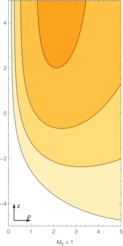
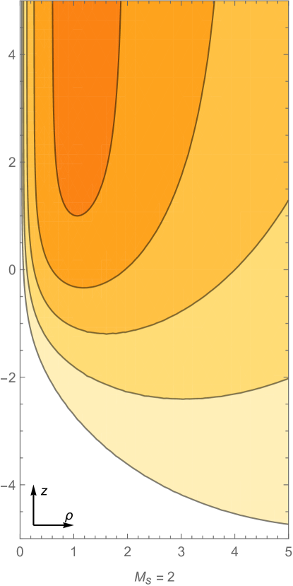
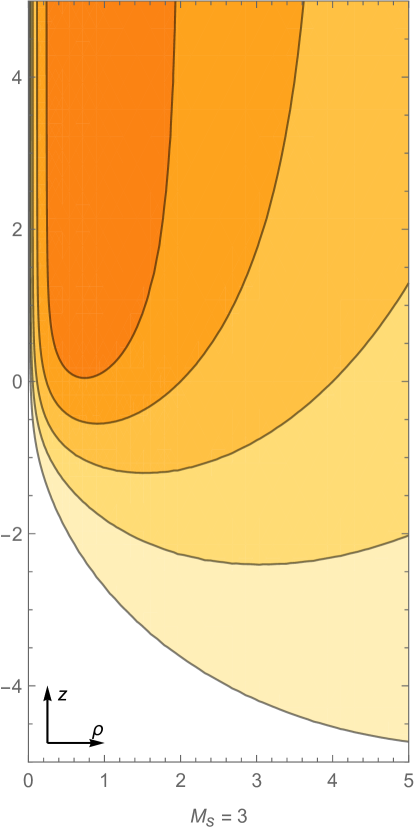
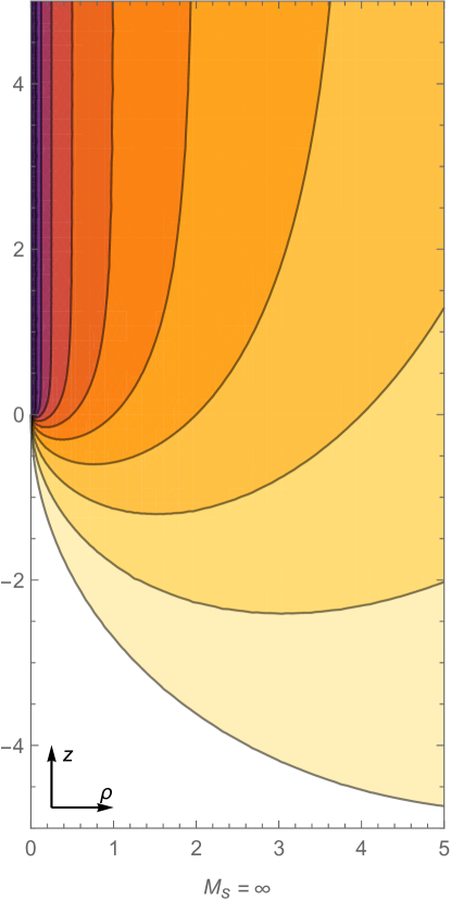
Figure 1: The metric function of the NUT-charged spacetime in the infinite derivative gravity. We plot the contours of ${V/\rho N}$ for different values of the non-local scale $M_{\textrm{s}}$. The function is finite everywhere for finite values of $M_{\textrm{s}}$, but diverges toward the top semi-axis (the Misner string) in the local limit, ${M_{\textrm{s}}=\infty}$.

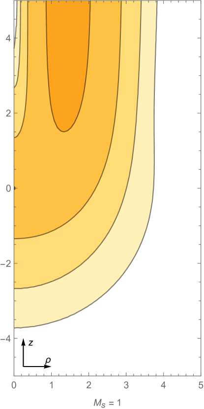
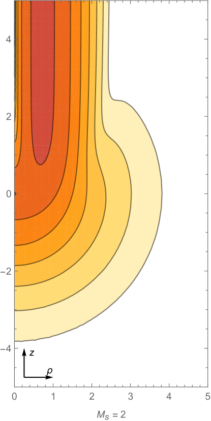
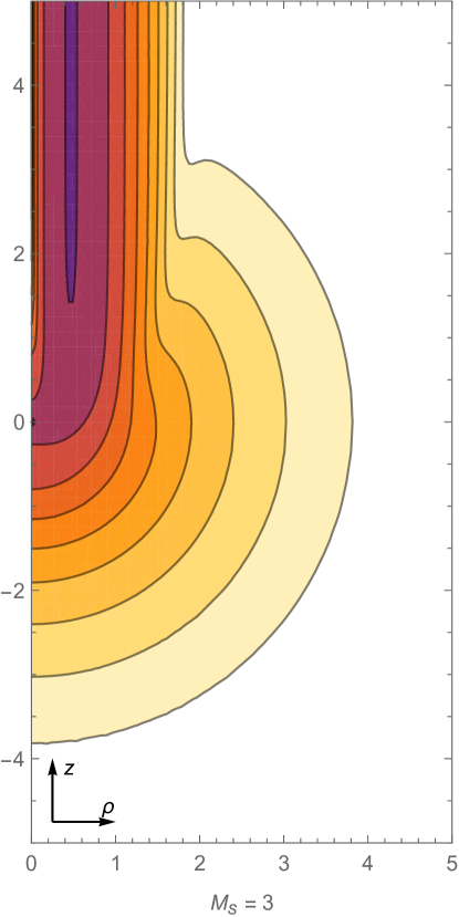
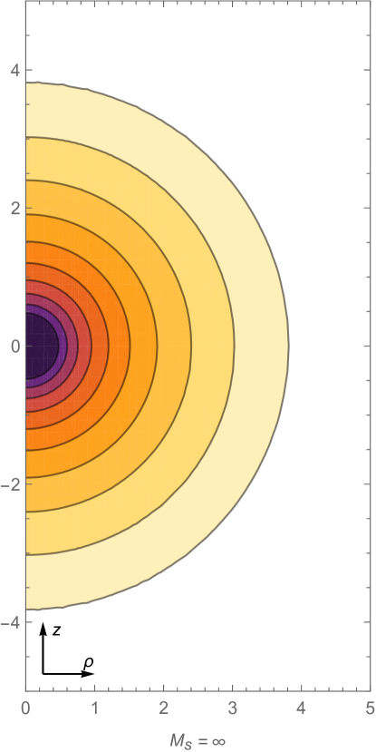
Figure 2: The Kretschmann scalar of the NUT-charged spacetime in the infinite derivative gravity. We plot the contours of $\sqrt{-K}/|N|$ for different values of the non-local scale $M_{\textrm{s}}$. The Kretschmann scalar is finite everywhere for finite $M_{\textrm{s}}$. With the increasing value of $M_{\textrm{s}}$, the curvature accumulates along the top semi-axis and gives rise to distributional curvature (the Misner string) in the local limit, ${M_{\textrm{s}}=\infty}$, for which the Kretschmann scalar also diverges at the origin.

III.2 Curvature

To the first order in metric perturbation ${h_{\mu\nu}}$, the Riemann tensor, the Ricci tensor, and the Ricci scalar in the harmonic gauge (7) read

$$\begin{gathered}R_{\mu\nu\rho\sigma}=\partial_{\nu}\partial_{[\rho}h_{\sigma]\mu}-\partial_{\mu}\partial_{[\rho}h_{\sigma]\nu}\;,\\ \ R_{\mu\nu}=-\frac{1}{2}\Box h_{\mu\nu}\;,\quad R=-\frac{1}{2}\Box h\;.\end{gathered}$$ (41)

Using the metric ansatz (19) together with (20), we find the non-trivial component expressed in terms of metric functions $X$ and $Y$:

$$\begin{gathered}\begin{aligned} R_{txxy}&=\frac{1}{2}\partial^{2}Y\;,&\quad R_{tyyx}&=\frac{1}{2}\partial^{2}X\;,\\ R_{txxz}&=-\frac{1}{2}\partial_{x}\partial_{z}X\;,&\quad R_{tyyz}&=-\frac{1}{2}\partial_{y}\partial_{z}Y\;,\\ R_{txyz}&=-\frac{1}{2}\partial_{x}\partial_{z}Y\;,&\quad R_{tyxz}&=-\frac{1}{2}\partial_{y}\partial_{z}X\;,\\ R_{tzxz}&=-\frac{1}{2}\partial_{z}^{2}X\;,&\quad R_{tzyz}&=-\frac{1}{2}\partial_{z}^{2}Y\;,\end{aligned}\\ R_{tzxy}=\frac{1}{2}(-\partial_{y}\partial_{z}X+\partial_{x}\partial_{z}Y)\;,\\ R_{tx}=-\frac{1}{2}\Delta X\;,\quad R_{ty}=-\frac{1}{2}\Delta Y\;,\quad R=0\;,\end{gathered}$$ (42)

where we introduced the two-dimensional Laplacian operator ${\partial^{2}\equiv\partial_{x}^{2}+\partial_{y}^{2}}$.

Note that all the components of the Riemann tensor (including all combinations of covariant and contravariant indices) are finite everywhere. This already implies that there is no curvature singularity or topological defect such as the Misner string in the spacetime. Nevertheless, to get simple invariant information about the curvature, we also compute the Kretschmann scalar ${K=R_{\mu\nu\rho\sigma}R^{\mu\nu\rho\sigma}}$ to the lowest order in metric perturbations. We express it in terms of the function $V$ by means of (24),

$$K =-2\Big{[}(\partial^{2}X)^{2}+(\partial^{2}Y)^{2}+(\partial_{z}^{2}X)^{2}+(\partial_{z}^{2}Y)^{2}$$ (43)

$$\mathrel{\phantom{=}}+(\partial_{x}\partial_{z}X)^{2}+(\partial_{y}\partial_{z}Y)^{2}+(\partial_{y}\partial_{z}X)^{2}+(\partial_{x}\partial_{z}Y)^{2}$$

$$\mathrel{\phantom{=}}+(\partial_{y}\partial_{z}X+\partial_{x}\partial_{z}Y)^{2}\Big{]}$$

$$=-\frac{1}{4v^{2}}\big{[}2v^{3}(\partial_{v}^{2}V)^{2}+3v^{2}(\partial_{v}\partial_{z}V)^{2}+2v(\partial_{z}^{2}V)^{2}$$

$$\mathrel{\phantom{=}}+(v\partial_{v}\partial_{z}V-\partial_{z}V)^{2}\big{]}\;,$$

where we can observe that ${K\leq 0}$. Inserting (36) in (43), we obtain

$$K =-\frac{2N^{2}}{\pi\,r^{6}z^{2}}\Big{[}M_{\textrm{s}}^{6}\rho^{2}r^{4}\big{(}r^{2}\beta(\tfrac{M_{\textrm{s}}z}{2})^{2}{-}2\rho^{2}\beta(\tfrac{M_{\textrm{s}}z}{2}){+}r^{2}\big{)}$$ (44)

$$\mathrel{\phantom{=}}+12z^{2}\alpha(\tfrac{M_{\textrm{s}}r}{2})\big{(}2\alpha(\tfrac{M_{\textrm{s}}r}{2}){-}M_{\textrm{s}}^{3}\rho^{2}r\beta(\tfrac{M_{\textrm{s}}z}{2})\big{)}\Big{]}e^{-M_{\textrm{s}}^{2}r^{2}/2}\;,$$

where $\alpha$ and $\beta$ are functions defined by

$$\alpha(w) =\sqrt{\pi}\operatorname{erf}(w)e^{w^{2}}-2w\;,$$ (45)

$$\beta(w) =\sqrt{\pi}\big{(}1+\operatorname{erf}(w)\big{)}we^{w^{2}}+1\;.$$

Examining the limits ${r\to 0}$ and ${z\to 0}$, one can verify that the Kretschmann scalar is also finite everywhere.

It is interesting to investigate the local limit of the Kretschmann scalar. Outside the axis of symmetry we see that it reduces to the Kretschmann scalar of the Taub–NUT spacetime,

$$\lim_{M_{\textrm{s}}\to\infty}K=K_{\textrm{loc}}=-\frac{48N^{2}}{r^{3}}\;,\quad\rho>0\;,$$ (46)

which diverges toward the origin ${r=0}$. Note that this is a feature of the linearized Taub–NUT only. The Kretschmann scalar is depicted in the contour plots in Fig. 2. Inspecting the graphs for increasing values of the non-local scale ${M_{\textrm{s}}}$, we see that the curvature really accumulates around the top axis. This can be viewed as a process in which the Misner string corresponding to distributional curvature arises in the local limit.

III.3 Asymptotic regions: ${z\to\pm\infty}$

Let us explore asymptotic limits of the spacetime for large positive and negatives values of coordinate $z$, which correspond to the far region around the top and the bottom semi-axes, respectively. In these asymptotic regions, the function $V$ becomes independent of $z$, and it can be simply approximated by its limits,

$$\lim_{z\to\pm\infty}V=\begin{cases}4N\big{(}1-e^{-M_{\textrm{s}}^{2}\rho^{2}/4}\big{)}\equiv\overline{V}\;,\\ 0\;.\end{cases}$$ (47)

The geometry approaches Minkowski spacetime in the bottom part and the spacetime of the spinning cosmic string of an infinite length in the top section. The latter is generated by the infinite linear source (18) with angular momentum ${J=N}$, which was recently found in Boos (2020). The asymptotic geometry given by ${\overline{V}}$ approaches the solution of the local theory (17) with ${J=N}$ far from the axis because

$$\overline{V}\approx 4N\equiv\overline{V}_{\textrm{loc}}\;,\quad\rho\gg 1/M_{\textrm{s}}\;.$$ (48)

Naturally, $\overline{V}$ reduces to this solution in the local limit ${M_{\textrm{s}}\to\infty}$ as well,

$$\lim_{M_{\textrm{s}}\to\infty}\overline{V}=\overline{V}_{\textrm{loc}}\;,\quad\rho>0\;.$$ (49)

As before, the functions ${\bar{X}}$ and ${\bar{Y}}$ are finite everywhere in contrast to ${\bar{X}_{\textrm{loc}}}$ and ${\bar{Y}_{\textrm{loc}}}$. The function ${\overline{V}/\rho N}$ is visualized in Fig. 3.

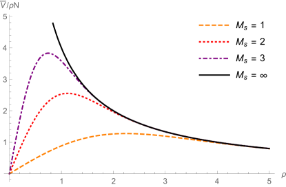
Figure 3: The metric function of the spinning cosmic string spacetime in the infinite derivative gravity. We plot the function ${\overline{V}/\rho N}$ for different values of non-local scale $M_{\textrm{s}}$. The function is finite everywhere for finite values of ${M_{\textrm{s}}}$, but diverges toward ${\rho=0}$ in the local limit, ${M_{\textrm{s}}=\infty}$.

The Kretschmann scalar can be obtained by ignoring the terms with $\partial_{z}$ in (43),

$$\overline{K} =-2\big{[}(\partial^{2}\overline{X})^{2}+(\partial^{2}\overline{Y})^{2}\big{]}=-\frac{v}{2}(\partial_{v}^{2}\overline{V})^{2}$$ (50)

$$=-2M_{\textrm{s}}^{8}N^{2}\rho^{2}e^{-M_{\textrm{s}}^{2}\rho^{2}/2}\;.$$

As expected, it vanishes everywhere outside the axis in the local limit

$$\lim_{M_{\textrm{s}}\to\infty}\overline{K}=\overline{K}_{\textrm{loc}}=0\;,\quad\rho>0\;,$$ (51)

because the spacetime of the spinning cosmic string is locally flat for ${\rho>0}$. This analysis again confirms that the curvature really accumulates along the axis in the local limit as one can also see from the graphs of the Kretschmann scalar in Fig. 4.

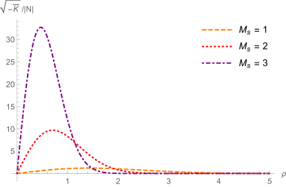
Figure 4: The Kretschmann scalar of the spinning cosmic string spacetime in the infinite derivative gravity. We plot $\sqrt{-\overline{K}}/|N|$ for different values of non-local scale $M_{\textrm{s}}$. The Kretschman scalar is finite everywhere for finite ${M_{\textrm{s}}}$. With the increasing value of ${M_{\textrm{s}}}$, the curvature accumulates at ${\rho=0}$ as described in (52).

Finally, it is worth to mention that if we approximate the Dirac delta function by the Gaussian function ${\delta(x)\approx e^{-x^{2}/\epsilon^{2}}/\sqrt{\pi}\epsilon}$, ${0<\epsilon\ll 1}$, then the field equations imply

$$\sqrt{-\overline{K}_{\textrm{loc}}} =\sqrt{2\big{[}(\partial^{2}\overline{X}_{\textrm{loc}})^{2}{+}(\partial^{2}\overline{Y}_{\textrm{loc}})^{2}\big{]}}$$ (52)

$$\approx 2^{9/2}|N|\epsilon^{-4}\rho e^{-\rho^{2}/\epsilon^{2}}$$

$$\approx-8\sqrt{2}\pi|N|\,\partial_{\rho}\big{(}\delta(x)\delta(y)\big{)}\;,\quad 0<\epsilon\ll 1\;.$$

Comparing (52) with (50), we can see that ${\epsilon=2/M_{\textrm{s}}}$, for ${M_{\textrm{s}}\gg 1}$. This very sloppy calculation indicates how distributional curvature arises in the local limit.

IV Conclusions

The Taub–NUT spacetime has recently regained significant attention as several presumed unphysical properties have been disproved. In this paper, we studied NUT charge in the context of linearized infinite derivative gravity. We found an analytic solution which is regular everywhere due to the presence of the non-local form-factor, which effectively smears the distributional source. Our analysis of the Riemann tensor and Kretschmann scalar shows the absence of curvature singularities as well as topological defects such as the Misner string. The obtained geometry reduces to the linearized Taub–NUT spacetime far from the source and in the local limit. We also investigated the asymptotic limit along the axis, which gives rise to the non-local version of the spinning infinite string spacetime. Our results extend the set of papers on the linearized solutions by the NUT-charged solution.

A natural next step is to investigate further properties of the NUT charge in infinite derivative gravity. An example is the presence of the closed timelike curves and the existence of the horizons. Unfortunately, these problems are challenging since a full non-linear approach is required. Our knowledge of the exact solutions in this theory is still very sparse, but there are already many hints that might help us make progress in this direction.

Nevertheless, even at the level of linearized theory, there are still many interesting solutions of the general relativity that might have their counterparts in the infinite derivative gravity. As mentioned in the introduction, the linearized solutions in the non-local theories may actually play more important role than in the local theories.

Our discussion of the presence of singularities is based on the linearized theory. However, it is expected that even the full non-linear theory does not admit singular solutions. The field equations of the full theory involve non-local form-factors acting on the curvature tensors. These operators typically smear the distribution curvature and produce smooth functions. It is anticipated that this mechanism could prevent vacuum solutions (with distributional stress-energy tensor) of local theories with polynomial form-factors to be vacuum solutions of non-local theories. Unfortunately, satisfactory proofs of such statements are still lacking even for very simple examples of singular spacetimes. Nevertheless, the absence of singularities is already partially hinted by the existence of bouncing cosmological solutions Biswas et al. (2006) and approximate spherically symmetric solutions that are valid in the region where non-locality is important Buoninfante et al. (2018b).

References

- Will (2014) Clifford M. Will, “The Confrontation between General Relativity and Experiment,” Living Rev. Rel. 17, 4 (2014), arXiv:1403.7377 [gr-qc] .
- Stelle (1978) K. S. Stelle, “Classical Gravity with Higher Derivatives,” Gen. Rel. Grav. 9, 353–371 (1978).
- Stelle (1977) K.S. Stelle, “Renormalization of Higher Derivative Quantum Gravity,” Phys. Rev. D 16, 953–969 (1977).
- Asorey et al. (1997) M. Asorey, J.L. Lopez, and I.L. Shapiro, “Some remarks on high derivative quantum gravity,” Int. J. Mod. Phys. A 12, 5711–5734 (1997), arXiv:hep-th/9610006 .
- Modesto et al. (2015) Leonardo Modesto, Tibério de Paula Netto, and Ilya L. Shapiro, “On Newtonian singularities in higher derivative gravity models,” JHEP 04, 098 (2015), arXiv:1412.0740 [hep-th] .
- Giacchini and de Paula Netto (2019) Breno L. Giacchini and Tibério de Paula Netto, “Effective delta sources and regularity in higher-derivative and ghost-free gravity,” JCAP 1907, 013 (2019), arXiv:1809.05907 [gr-qc] .
- Witten (1986) Edward Witten, “Noncommutative Geometry and String Field Theory,” Nucl. Phys. B268, 253–294 (1986).
- Freund and Olson (1987) Peter G. O. Freund and Mark Olson, “Nonarchimedean strings,” Phys. Lett. B199, 186–190 (1987).
- Freund and Witten (1987) Peter G.O. Freund and Edward Witten, “Adelic string amplitudes,” Phys. Lett. B 199, 191 (1987).
- Brekke et al. (1988) Lee Brekke, Peter G. O. Freund, Mark Olson, and Edward Witten, “Nonarchimedean String Dynamics,” Nucl. Phys. B302, 365–402 (1988).
- Frampton and Okada (1988) Paul H. Frampton and Yasuhiro Okada, “Effective Scalar Field Theory of adic String,” Phys. Rev. D37, 3077–3079 (1988).
- Biswas et al. (2012a) Tirthabir Biswas, Erik Gerwick, Tomi Koivisto, and Anupam Mazumdar, “Towards singularity and ghost free theories of gravity,” Phys. Rev. Lett. 108, 031101 (2012a), arXiv:1110.5249 [gr-qc] .
- Biswas et al. (2013) Tirthabir Biswas, Tomi Koivisto, and Anupam Mazumdar, “Nonlocal theories of gravity: the flat space propagator,” in Proceedings, Barcelona Postgrad Encounters on Fundamental Physics (2013) pp. 13–24, arXiv:1302.0532 [gr-qc] .
- Biswas et al. (2014) Tirthabir Biswas, Aindriú Conroy, Alexey S. Koshelev, and Anupam Mazumdar, “Generalized ghost-free quadratic curvature gravity,” Class. Quant. Grav. 31, 015022 (2014), [Erratum: Class. Quant. Grav.31,159501(2014)], arXiv:1308.2319 [hep-th] .
- Modesto (2012) Leonardo Modesto, “Super-renormalizable Quantum Gravity,” Phys. Rev. D86, 044005 (2012), arXiv:1107.2403 [hep-th] .
- Modesto (2013) Leonardo Modesto, “Super-renormalizable Multidimensional Quantum Gravity,” Astron. Rev. 8, 4–33 (2013), arXiv:1202.3151 [hep-th] .
- Tomboulis (1997) E. T. Tomboulis, “Superrenormalizable gauge and gravitational theories,” (1997), arXiv:hep-th/9702146 [hep-th] .
- Modesto and Rachwal (2014) Leonardo Modesto and Leslaw Rachwal, “Super-renormalizable and finite gravitational theories,” Nucl. Phys. B889, 228–248 (2014), arXiv:1407.8036 [hep-th] .
- Talaganis et al. (2015) Spyridon Talaganis, Tirthabir Biswas, and Anupam Mazumdar, “Towards understanding the ultraviolet behavior of quantum loops in infinite-derivative theories of gravity,” Class. Quant. Grav. 32, 215017 (2015), arXiv:1412.3467 [hep-th] .
- Tomboulis (2015) E.T. Tomboulis, “Renormalization and unitarity in higher derivative and nonlocal gravity theories,” Mod. Phys. Lett. A 30, 1540005 (2015).
- Modesto et al. (2018) Leonardo Modesto, Lesł aw Rachwał, and Ilya L. Shapiro, “Renormalization group in super-renormalizable quantum gravity,” Eur. Phys. J. C 78, 555 (2018), arXiv:1704.03988 [hep-th] .
- Buoninfante et al. (2019) Luca Buoninfante, Gaetano Lambiase, and Anupam Mazumdar, “Ghost-free infinite derivative quantum field theory,” Nucl. Phys. B 944, 114646 (2019), arXiv:1805.03559 [hep-th] .
- Biswas et al. (2006) Tirthabir Biswas, Anupam Mazumdar, and Warren Siegel, “Bouncing universes in string-inspired gravity,” JCAP 0603, 009 (2006), arXiv:hep-th/0508194 [hep-th] .
- Koshelev et al. (2018a) Alexey S. Koshelev, K. Sravan Kumar, and Alexei A. Starobinsky, “ inflation to probe non-perturbative quantum gravity,” JHEP 03, 071 (2018a), arXiv:1711.08864 [hep-th] .
- Sravan Kumar and Modesto (2018) K. Sravan Kumar and Leonardo Modesto, “Non-local Starobinsky inflation in the light of future CMB,” (2018), arXiv:1810.02345 [hep-th] .
- Biswas et al. (2010) Tirthabir Biswas, Tomi Koivisto, and Anupam Mazumdar, “Towards a resolution of the cosmological singularity in non-local higher derivative theories of gravity,” JCAP 1011, 008 (2010), arXiv:1005.0590 [hep-th] .
- Biswas et al. (2012b) Tirthabir Biswas, Alexey S. Koshelev, Anupam Mazumdar, and Sergey Yu. Vernov, “Stable bounce and inflation in non-local higher derivative cosmology,” JCAP 1208, 024 (2012b), arXiv:1206.6374 [astro-ph.CO] .
- Koshelev et al. (2019) Alexey S. Koshelev, João Marto, and Anupam Mazumdar, “Towards resolution of anisotropic cosmological singularity in infinite derivative gravity,” JCAP 1902, 020 (2019), arXiv:1803.07072 [gr-qc] .
- Frolov and Zelnikov (2016) Valeri P. Frolov and Andrei Zelnikov, “Head-on collision of ultrarelativistic particles in ghost-free theories of gravity,” Phys. Rev. D93, 064048 (2016), arXiv:1509.03336 [hep-th] .
- Frolov et al. (2015) Valeri P. Frolov, Andrei Zelnikov, and Tibério de Paula Netto, “Spherical collapse of small masses in the ghost-free gravity,” JHEP 06, 107 (2015), arXiv:1504.00412 [hep-th] .
- Frolov (2015) Valeri P. Frolov, “Mass-gap for black hole formation in higher derivative and ghost free gravity,” Phys. Rev. Lett. 115, 051102 (2015), arXiv:1505.00492 [hep-th] .
- Edholm et al. (2016) James Edholm, Alexey S. Koshelev, and Anupam Mazumdar, “Behavior of the Newtonian potential for ghost-free gravity and singularity-free gravity,” Phys. Rev. D94, 104033 (2016), arXiv:1604.01989 [gr-qc] .
- Buoninfante et al. (2018a) Luca Buoninfante, Alexey S. Koshelev, Gaetano Lambiase, and Anupam Mazumdar, “Classical properties of non-local, ghost- and singularity-free gravity,” JCAP 1809, 034 (2018a), arXiv:1802.00399 [gr-qc] .
- Koshelev et al. (2018b) Alexey S. Koshelev, João Marto, and Anupam Mazumdar, “Schwarzschild -singularity is not permissible in ghost free quadratic curvature infinite derivative gravity,” Phys. Rev. D98, 064023 (2018b), arXiv:1803.00309 [gr-qc] .
- Buoninfante et al. (2018b) Luca Buoninfante, Alexey S. Koshelev, Gaetano Lambiase, João Marto, and Anupam Mazumdar, “Conformally-flat, non-singular static metric in infinite derivative gravity,” JCAP 1806, 014 (2018b), arXiv:1804.08195 [gr-qc] .
- Buoninfante et al. (2018c) Luca Buoninfante, Gerhard Harmsen, Shubham Maheshwari, and Anupam Mazumdar, “Nonsingular metric for an electrically charged point-source in ghost-free infinite derivative gravity,” Phys. Rev. D98, 084009 (2018c), arXiv:1804.09624 [gr-qc] .
- Buoninfante et al. (2018d) Luca Buoninfante, Alan S. Cornell, Gerhard Harmsen, Alexey S. Koshelev, Gaetano Lambiase, João Marto, and Anupam Mazumdar, “Towards nonsingular rotating compact object in ghost-free infinite derivative gravity,” Phys. Rev. D98, 084041 (2018d), arXiv:1807.08896 [gr-qc] .
- Boos et al. (2018) Jens Boos, Valeri P. Frolov, and Andrei Zelnikov, “Gravitational field of static p -branes in linearized ghost-free gravity,” Phys. Rev. D97, 084021 (2018), arXiv:1802.09573 [gr-qc] .
- Boos (2020) Jens Boos, “Angle deficit & non-local gravitoelectromagnetism around a slowly spinning cosmic string,” (2020), arXiv:2003.13847 [gr-qc] .
- Boos et al. (2020) Jens Boos, Jose Pinedo Soto, and Valeri P. Frolov, “Ultrarelativistic spinning objects (gyratons) in non-local ghost-free gravity,” (2020), arXiv:2004.07420 [gr-qc] .
- Taub (1951) A.H. Taub, “Empty space-times admitting a three parameter group of motions,” Annals Math. 53, 472–490 (1951).
- Newman et al. (1963) E. Newman, L. Tamburino, and T. Unti, “Empty space generalization of the Schwarzschild metric,” J. Math. Phys. 4, 915 (1963).
- Dowker and Roche (1967) J.S. Dowker and J.A. Roche, “The Gravitational analogues of magnetic monopoles,” Proc. Phys. Soc. 92, 1–8 (1967).
- Dirac (1931) Paul Adrien Maurice Dirac, “Quantised singularities in the electromagnetic field,,” Proc. Roy. Soc. Lond. A A133, 60–72 (1931).
- Misner (1963) Charles W. Misner, “The Flatter regions of Newman, Unti and Tamburino’s generalized Schwarzschild space,” J. Math. Phys. 4, 924–938 (1963).
- Bonnor (1969) W. B. Bonnor, “A new interpretation of the NUT metric in general relativity,” Mathematical Proceedings of the Cambridge Philosophical Society 66, 145–151 (1969).
- Sackfield (1971) A. Sackfield, “Physical interpretation of n.u.t. metric,” Mathematical Proceedings of the Cambridge Philosophical Society 70, 89–94 (1971).
- Bonnor (1992) W. B. Bonnor, “Physical interpretation of vacuum solutions of einstein’s equations. part i. time-independent solutions,” General Relativity and Gravitation 24, 551–574 (1992).
- Griffiths and Podolsky (2009) Jerry B. Griffiths and Jiri Podolsky, Exact Space-Times in Einstein’s General Relativity, Cambridge Monographs on Mathematical Physics (Cambridge University Press, Cambridge, 2009).
- Kolář and Krtouš (2019) Ivan Kolář and Pavel Krtouš, “Symmetry axes of Kerr-NUT-(A)dS spacetimes,” Phys. Rev. D 100, 064014 (2019), arXiv:1905.06585 [gr-qc] .
- Clément et al. (2015) Gérard Clément, Dmitri Gal’tsov, and Mourad Guenouche, “Rehabilitating space-times with NUTs,” Phys. Lett. B 750, 591–594 (2015), arXiv:1508.07622 [hep-th] .
- Gera and Sengupta (2019) Suvikranth Gera and Sandipan Sengupta, “Taming Dirac Strings and Timelike Loops in Vacuum Gravity,” Phys. Rev. D 99, 124038 (2019), arXiv:1902.07748 [gr-qc] .
- Hennigar et al. (2019) Robie A. Hennigar, David Kubizňák, and Robert B. Mann, “Thermodynamics of Lorentzian Taub-NUT spacetimes,” Phys. Rev. D 100, 064055 (2019), arXiv:1903.08668 [hep-th] .
- Bordo et al. (2019) Alvaro Ballon Bordo, Finnian Gray, Robie A. Hennigar, and David Kubizňák, “Misner Gravitational Charges and Variable String Strengths,” Class. Quant. Grav. 36, 194001 (2019), arXiv:1905.03785 [hep-th] .
- Luna et al. (2015) Andrés Luna, Ricardo Monteiro, Donal O’Connell, and Chris D. White, “The classical double copy for Taub–NUT spacetime,” Phys. Lett. B 750, 272–277 (2015), arXiv:1507.01869 [hep-th] .
- Biswas et al. (2016) Tirthabir Biswas, Alexey S. Koshelev, and Anupam Mazumdar, “Gravitational theories with stable (anti-)de Sitter backgrounds,” Fundam. Theor. Phys. 183, 97–114 (2016), arXiv:1602.08475 [hep-th] .
- Biswas et al. (2017) Tirthabir Biswas, Alexey S. Koshelev, and Anupam Mazumdar, “Consistent higher derivative gravitational theories with stable de Sitter and anti–de Sitter backgrounds,” Phys. Rev. D95, 043533 (2017), arXiv:1606.01250 [gr-qc] .
- Argurio and Dehouck (2010) Riccardo Argurio and Francois Dehouck, “Gravitational duality and rotating solutions,” Phys. Rev. D 81, 064010 (2010), arXiv:0909.0542 [hep-th] .
- Deser et al. (1984) Stanley Deser, R. Jackiw, and Gerard ’t Hooft, “Three-Dimensional Einstein Gravity: Dynamics of Flat Space,” Annals Phys. 152, 220 (1984).
- Mazur (1986) P.O. Mazur, “Spinning Cosmic Strings and Quantization of Energy,” Phys. Rev. Lett. 57, 929–932 (1986).
- Jensen and Soleng (1992) B. Jensen and H.H. Soleng, “General relativistic model of a spinning cosmic string,” Phys. Rev. D 45, 3528–3533 (1992).
- Galtsov and Letelier (1993) D.V. Galtsov and P.S. Letelier, “Spinning strings and cosmic dislocations,” Phys. Rev. D 47, 4273–4276 (1993).
- Tod (1994) K P Tod, “Conical singularities and torsion,” Classical and Quantum Gravity 11, 1331–1339 (1994).
- Puntigam and Soleng (1997) Roland A. Puntigam and Harald H. Soleng, “Volterra distortions, spinning strings, and cosmic defects,” Class. Quant. Grav. 14, 1129–1149 (1997), arXiv:gr-qc/9604057 .
- Vilenkin and Shellard (2000) A. Vilenkin and E.P. S. Shellard, Cosmic Strings and Other Topological Defects (Cambridge University Press, 2000).
- Otway (2012) Thomas H. Otway, The Dirichlet Problem for Elliptic-Hyperbolic Equations of Keldysh Type (Springer Berlin Heidelberg, 2012).
- Ng and Geller (1969) Edward W. Ng and Murray Geller, “A table of integrals of the error functions,” Journal of Research of the National Bureau of Standards, Section B: Mathematical Sciences 73B, 1 (1969).