Simulation and optimal control of the Williams-Otto process using Pyomo

Abstract

We illustrate the advantages the high-level open-source software package Pyomo has in rapidly setting up and solving dynamic simulation and optimization problems. In order to do so, we use the example of the Williams-Otto process. We show how to simulate the process dynamics using the collocation method and the IPOPT solver provided by Pyomo. We also discuss waste minimization and yield maximization as two examplary process optimization problems. And finally, we present and compare two approaches to setpoint tracking: one based on proportional-integral feedback control and one based on optimal open-loop control.

Index terms: dynamic simulation and optimization, control, optimal control, setpoint tracking, Williams-Otto process, Pyomo

1 Introduction

Virtualization permeates many aspects of chemical engineering nowadays. Computer models allow process optimization without the costs associated with experiments. And conversely, parameter estimation and machine learning methods allow experimental data to be fed back into computer models, increasing their reliability.

Chemical process models can be static (steady-state) or dynamic. Capturing the dynamic aspect becomes increasingly important if the process is supposed to adapt to external changes, such as fluctuations in supply, demand or energy cost. A prominent example of a method based on a dynamic model of the process is model-predictive control [1], [16], [18]. In case its underlying dynamic model is accurate enough, model-predictive control has the potential for smoother and thus more efficient adaptations compared to simple feedback loops like proportional-integral-derivative controllers. In spite of these drawbacks, proportional-integral-derivative controllers are still dominant in the process industries due to their simplicity [31] – but in recent years, with the advent of faster and faster optimization solvers (Table 2 and 3 of [3]), linear and nonlinear model-predictive control has found more and more industrial applications as well [16]. In particular, model-predictive control will probably be used more systematically in online optimization [17], which could replace the standard industrial real-time optimization solutions based on static process models that are currently offered by many vendors and used by the process industry.

A dynamic model can be the basis for a process optimization (optimal control) or data fitting task (parameter estimation). In either case, we obtain a so-called dynamic optimization problem [6]

$$\min J(\bm{x},\bm{u},\bm{p})$$ (1.1)

$$\bm{f}(\dot{\bm{x}}(t),\bm{x}(t),\bm{u}(t),\bm{p},t)=0\qquad(t\in[0,t_{f}])$$ (1.2)

$$\bm{g}(\bm{x}(t),\bm{u}(t),\bm{p},t)\leq 0\qquad(t\in[0,t_{f}]).$$ (1.3)

where we distinguish between state trajectories $\bm{x}$, control profiles $\bm{u}$ to be optimized, and time-independent finite-dimensional parameters $\bm{p}$ to be optimized. Sometimes, the final time $t_{f}$ is an optimization variable as well, in which case it has to be added to the goal function $J$’s list of arguments, but we will not consider that in the present paper. In chemical engineering applications, the control profiles $\bm{u}$ can be the temperature profile in a reactor or the reflux ratio profile in a batch distillation column [5], [14]. And the time-independent parameters $\bm{p}$ will typically be model parameters – like reaction rates [30] or equlibrium model parameters [10] – or design parameters – like reactor length, diameter, inlet temperature and composition in reactor design, for instance. In the simplest case, the inequality constraints (1.3) just take the form of box constraints

$$\underline{\bm{x}}\leq\bm{x}(t)\leq\overline{\bm{x}},\qquad\underline{\bm{u}}\leq\bm{u}(t)\leq\overline{\bm{u}},\qquad\underline{\bm{p}}\leq\bm{p}\leq\overline{\bm{p}}\qquad(t\in[0,t_{f}])$$ (1.4)

with appropriate lower and upper bounds for the state and control variables $\bm{x},\bm{u}$ and the parameters $\bm{p}$. (As usual, for vectorial quantities, the above inequalities are to be understood componentwise.) Clearly, inequality constraints of the form (1.3) also comprise equality constraints – in the case of box constraints (1.4), for instance, one just has to choose identical lower and upper bounds. In many cases, the differential-algebraic constraints (1.2) can be separated into an ordinary differential equation for the states and additional algebraic equations, so that the optimal control problem (1.1)-(1.3) then takes the simpler form

$$\min J(\bm{x},\bm{u},\bm{p})$$ (1.5)

$$\dot{\bm{x}}(t)=\bm{f}(\bm{x}(t),\bm{u}(t),\bm{p},t)\qquad(t\in[0,t_{f}])$$ (1.6)

$$\bm{g}(\bm{x}(t),\bm{u}(t),\bm{p},t)\leq 0\qquad(t\in[0,t_{f}]).$$ (1.7)

Approaches to solve dynamic optimization problems as above can be distinguished according to how strongly the procedure of solving the differential equation is intertwined with the procedure of improving the goal function value. There is a whole spectrum of different approaches ranging from methods with weakly intertwined to methods with strongly intertwined solution and optimization procedures. Also, in recent years, a number of sophisticated software tools to solve dynamic optimization problems have emerged like Pyomo [21], [24], ACADO [22] and CasADi [3], for instance. See, for instance, [6] (Section 8.6) for a compact overview over the spectrum of solution approaches for dynamic optimization problems.

At the weakly intertwined end of the spectrum lies the so-called sequential approach. In this approach, a single step in the controls $\bm{u}$ and parameters $\bm{p}$ towards improvement of the objective function (for example in the direction of steepest descent) alternates with a complete solution of the differential equation, for example using a Runge-Kutta method.

At the strongly intertwined end of the spectrum lies the so-called simultaneous approach and, in particular, the collocation method used in Pyomo [21], [24]. In this approach, both states and controls are discretized simultaneously. The differential equation is then transformed into a system of equations by use of orthogonal collocation. The algebraic constraints are also transformed to a finite equation system. After this transformation, the discretized states and their derivatives, the discretized controls and the finite-dimensional parameters are all treated as optimization parameters within one large nonlinear optimization problem.

Somewhere in the middle between these two ends of the spectrum lies the multiple shooting [8], [15] approach used in ACADO [22]. In that approach, the time horizon $[0,t_{f}]$ of the states is partitioned. Similarly to the sequential approach, a single step towards improvement of the objective alternates with solving the differential equations for all partition intervals. However, the so-called matching conditions, which enforce continuity of the states from one partition interval to the next, are part of the optimization problem. This is achieved by treating the initial values for each partition interval as additional optimization parameters. Therefore, similarly to the collocation approach, the solution of the differential equation over the whole time horizon is obtained alongside the improvement of the objective, and only at convergence the solution $(\bm{x}^{*},\bm{u}^{*},\bm{p}^{*})$ is guaranteed to globally solve the differential equation.

2 Pyomo

Pyomo [20], [21], [24] was originally developed by researchers in the Center for Computing Research at Sandia National Laboratories and is a COIN-OR project. The software can be used to solve dynamic optimization problems as formulated in (1.1)-(1.2). In particular, with the pyomo.dae module it is possible to solve optimal control problems with differential-algebraic or even partial differential-algebraic equations (DAE or PDAE) as constraints [24].

Pyomo is based on Python, a popular high-level programming language. Aside from a small number of Pyomo-specific commands, no specific modelling language has to be learnt to start using it. The user defines the dynamic optimization problem in its original form (1.1)-(1.2) using constructs provided by Pyomo. For example, the time domain $[0,t_{f}]$ is introduced as a continuous set, and the states and their derivatives are identified as such by specific commands. Pyomo features automatic differentiation, so the user does not have to specify functions to return the derivatives of the objective function $J$ nor of the constraints $\bm{f}$ and $\bm{g}$.

Additionally, Pyomo provides two automatic discretization transformations: orthogonal collocation and finite differences. See [24], [21] or the Pyomo website for algorithmic details. Both transformations take a user-defined continuous model and discretize it automatically, that is, transform the dynamic optimization problem into a standard non-linear program composed of algebraic functions and equations. In particular, no manual discretziations are necessary, which removes many potential sources of errors.

Finally, the discretized optimization model is handed to the IPOPT solver included in Pyomo. IPOPT is a powerful state-of-the-art interior-point solver [34], [32], [33]. It should be noticed that the discretization transformation leads to a largely sparse algebraic system. Pyomo ensures that IPOPT makes use of this property when solving the discretized problem.

3 Simulation of the Williams-Otto process

3.1 Williams-Otto process

In this section, we introduce the process on which we illustrate the simulation framework from Section 2, namely the Williams-Otto process. The Williams-Otto process is an exemplary chemical process which comprises several common process units from chemical engineering and is therefore extensively studied in the literature [35], [23], [19], [13], [7].

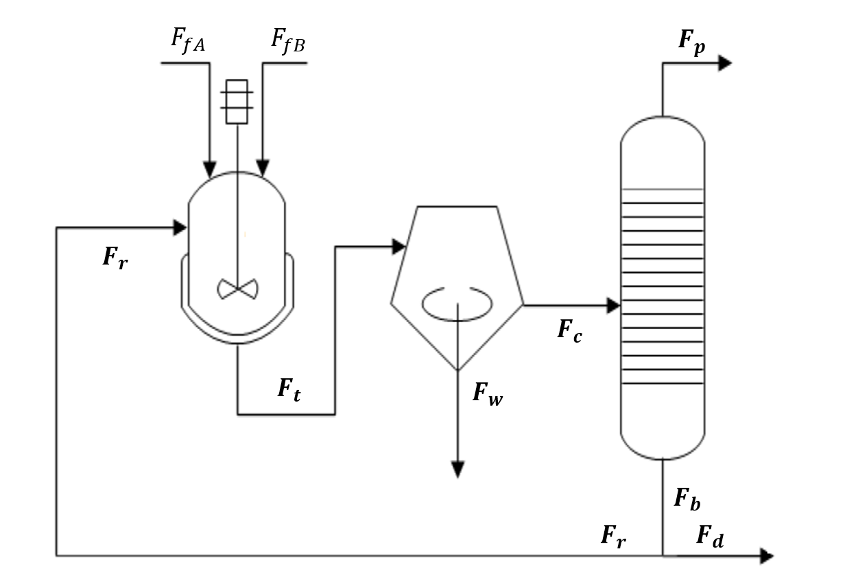
Figure 1: Williams-Otto process flowsheet (adapted from [13])

It consists of four subsystems: a continuously stirred tank reactor, a decanter (centrifuge), a distillation column (separator) and a splitter. See Figure 1 for a schematic flowsheet of the process. Two substances $A$ and $B$ are fed into the reactor (with mass streams $F_{fA}$ and $F_{fB}$ respectively), where they interact according to the following reaction system:

$$A+B\longrightarrow C$$ (3.1)

$$C+B\longrightarrow P+E$$ (3.2)

$$P+C\longrightarrow G$$ (3.3)

A compound mass stream $\bm{F}_{t}=(F_{tA},F_{tB},F_{tC},F_{tP},F_{tE},F_{tG})$ of total amount $\mu:=F_{tA}+\dotsb+F_{tG}$ then leaves the reactor. In the decanter, the waste product $G$ is removed from the process through a waste stream

$$F_{wG}=F_{tG}.$$ (3.4)

In the distillation column, part of the desired product $P$ is distilled with a fixed efficiency, namely

$$F_{pP}=F_{cP}-0.1F_{cE}=F_{tP}-0.1F_{tE}$$ (3.5)

where $\bm{F}_{c}$ is the input stream to the distillation column. The bottom stream $\bm{F}_{b}$ of the distillation column is partly withdrawn at a ratio $\eta$ (stream $\bm{F}_{d}$) and partly recycled back to the reactor at the ratio $1-\eta$ (stream $\bm{F}_{r}$). In total, there are five controls: the feed streams $F_{fA}$ and $F_{fB}$, the reactor temperature $T$, the total mass stream $\mu$ leaving the reactor, and the split fraction $\eta$. Also, there are six substances $A,B,C,P,E,G$ that interact in the reactor, and their masses inside the reactor are denoted by $m_{A},\dots,m_{G}$.

Applying the rules of reaction kinetics and using component mass balances around each of the four subsystems, one can derive the following system of ordinary differential equations for the masses $m_{A},\dots,m_{G}$ of the species in the reactor:

$$\dot{m}_{A} =F_{fA}+((1-\eta)\mu-\mu)\frac{m_{A}}{m}-k_{1}(T)\frac{m_{A}m_{B}}{V}$$ (3.6)

$$\dot{m}_{B} =F_{fB}+((1-\eta)\mu-\mu)\frac{m_{B}}{m}-k_{1}(T)\frac{m_{A}m_{B}}{V}-k_{2}(T)\frac{m_{B}m_{C}}{V}$$ (3.7)

$$\dot{m}_{C} =((1-\eta)\mu-\mu)\frac{m_{C}}{m}+2k_{1}(T)\frac{m_{A}m_{B}}{V}-2k_{2}(T)\frac{m_{B}m_{C}}{V}-k_{3}(T)\frac{m_{C}m_{P}}{V}$$ (3.8)

$$\dot{m}_{E} =((1-\eta)\mu-\mu)\frac{m_{E}}{m}+2k_{2}(T)\frac{m_{B}m_{C}}{V}$$ (3.9)

$$\dot{m}_{P} =0.1(1-\eta)\mu\frac{m_{E}}{m}-\mu\frac{m_{P}}{m}+k_{2}(T)\frac{m_{B}m_{C}}{V}-0.5k_{3}(T)\frac{m_{C}m_{P}}{V}$$ (3.10)

$$\dot{m}_{G} =-\mu\frac{m_{G}}{m}+1.5k_{3}(T)\frac{m_{C}m_{P}}{V},$$ (3.11)

In these equations, $m:=m_{A}+\dotsb+m_{G}$ and $V:=m_{A}/\rho_{A}^{0}+\dotsb+m_{G}/\rho_{G}^{0}$ denote the total mass and the total volume of the mixture in the reactor, respectively, with equal pure-substance densities $\rho_{A}^{0},\dots,\rho_{G}^{0}=50\,\mathrm{lb/ft^{3}}$ (Appendix I of [35]). Also, the reaction rates $k_{i}$ are given by

$$k_{i}(T)=\frac{a_{i}}{\rho}\,\mathrm{exp}(-b_{i}/T)\qquad(i\in\{1,2,3\})$$ (3.12)

where $a_{i}$, $b_{i}$, $\rho$ are the constants from [7] (Section 8.2.1):

$$a_{1}:=5.9755\cdot 10^{9}\,\mathrm{h}^{-1},\quad a_{2}:=2.5962\cdot 10^{12}\,\mathrm{h}^{-1},\quad a_{3}:=9.6283\cdot 10^{15}\,\mathrm{h}^{-1},$$ (3.13)

$$\rho:=50\,\mathrm{lb}/\mathrm{ft}^{3},\quad b_{1}:=12000\,\mathrm{{}^{\circ}R},\quad b_{2}:=15000\,\mathrm{{}^{\circ}R},\quad b_{3}:=20000\,\mathrm{{}^{\circ}R}$$ (3.14)

It is through these reaction rates that the reactor temperature $T$ – which is one of our controls – influences the process. In the entire paper, we adopt the common unit conventions from the Williams-Otto literature [35], [13], [7], that is, masses are measured in $\mathrm{klb}$, time is measured in $\mathrm{h}$, mass flows are measured in $\mathrm{klb/h}$, and temperatures are measured in ${}^{\circ}\mathrm{R}$ (degrees Réaumur).

We will often refer to (3.6)-(3.11) as the Williams-Otto equations in what follows. In view of the bilinear mass terms in the numerators and the total mass and total volume terms in the denominators on the right-hand sides of (3.6)-(3.11), the Williams-Otto equations are clearly nonlinear. With the abbreviations

$$\bm{x}(t):=(m_{A}(t),m_{B}(t),m_{C}(t),m_{E}(t),m_{P}(t),m_{G}(t)),$$ (3.15)

$$\bm{u}(t):=(F_{fA}(t),F_{fB}(t),T(t),\mu(t),\eta(t))$$ (3.16)

for the state and control variables, the Williams-Otto equations assume the standard form

$$\dot{\bm{x}}(t)=\bm{f}(\bm{x}(t),\bm{u}(t))$$ (3.17)

of a nonlinear time-invariant finite-dimensional control system. It can be shown that for every given initial state $\bm{x_{0}}$ and every given (bounded) control profile $\bm{u}$, the corresponding initial value problem

$$\dot{\bm{x}}(t)=\bm{f}(\bm{x}(t),\bm{u}(t))\qquad\text{and}\qquad\bm{x}(0)=\bm{x_{0}}$$ (3.18)

has a unique (local) solution in the sense of Carathéodory. See [28] (Lemma 2.6.2) or [11] (Section 3.2), for instance. All streams of the Williams-Otto process – except for the feed streams, of course – can be directly calculated from the solution of (3.6)-(3.11) and the tank outlet stream $\mu$: for example,

$$F_{tA}=\mu\frac{m_{A}}{m},\quad\dots\quad F_{tG}=\mu\frac{m_{G}}{m}.$$ (3.19)

3.2 Simulation examples

As has been pointed out in Section 2, implementing the Williams-Otto equations in Pyomo is fairly easy and convenient. In this subsection, we present two very simple simulation examples for the Williams-Otto process performed in Pyomo. In both examples, we start from the initial state $\bm{x_{0}}:=(10,1,0,0,0,0)$ and we impose a piecewise constant control input $\bm{u}$ with just one jump (step change) at the time $t^{*}:=100$, that is,

$$\bm{u}(t)=\bm{u}^{*}\quad(t\leq t^{*})\qquad\text{and}\qquad\bm{u}(t)=\bm{u}^{**}\quad(t>t^{*}).$$

Also, the initial part $\bm{u}^{*}$ of the control is the same in both examples, namely

$$F_{fA}^{*}:=10,\quad F_{fB}^{*}:=20,\quad T^{*}:=580,\quad\mu^{*}:=129.5,\quad\eta:=0.2.$$ (3.20)

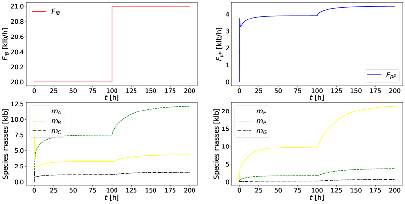
Figure 2: Step change in $F_{fB}$, response of $F_{pP}$ (top row), and resulting state trajectories (bottom row)

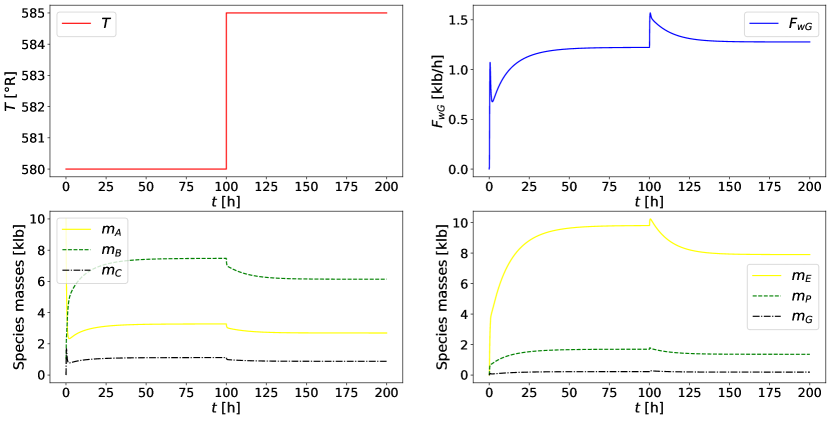
Figure 3: Step change in $T$, response of $F_{wG}$ (top row), and resulting state trajectories (bottom row)

In the first example (Figure 2), the step change is in the control variable $F_{fB}$, namely from $F_{fB}^{*}=20$ to $F_{fB}^{**}:=21$. And in the second example (Figure 3), the step change is in the $T$-profile, from $T^{*}=580$ to $T^{**}:=585$. It takes just about $1$ CPU second and $7$ IPOPT iterations to perform the above simulation examples (chosen number of finite elements and number of collocation points per finite element: $1500$ and $3$, respectively). We see that before and long after the jump, the state trajectories become flat (Figure 2 and 3 (bottom row)). In other words, at those times, the Williams-Otto process is in steady-state operation.

4 Setpoint tracking by means of proportional-integral control

An important task in process engineering is setpoint tracking, that is, to steer a process from a steady state to another steady state in such a way that a chosen process quantity of interest – the so-called setpoint quantity – asymptotically approaches a user-specified setpoint. In our Williams-Otto example, typical setpoint quantities are the product stream $F_{pP}$ from the head of the distillation column and the waste stream $F_{wG}$ from the bottom of the decanter.

A standard approach to perform setpoint tracking is to use proportional-integral controllers. Such a controller – just like any other controller – is based on an appropriately designed feedback relation between the setpoint quantity $y$ in question and an appropriate corresponding control quantity $u$. In formulas, the feedback relation of a proportional-integral controller looks as follows:

$$u(t)=u^{bias}+K^{prop}(y^{sp}-y(t))+K^{int}\int_{t^{*}}^{t}(y^{sp}-y(\tau))\,\mathrm{d}\tau$$ (4.1)

for $t>t^{*}$, that is, $t^{*}$ is the time where the feedback loop between setpoint and control quantity is activated. We immediately see from this formula that the control action $u(t)$ is the larger, the larger the current and the cumulated deviation

$$y^{sp}-y(t),\qquad\int_{t^{*}}^{t}(y^{sp}-y(\tau))\,\mathrm{d}\tau$$ (4.2)

of our setpoint quantity $y$ from the user-specified setpoint $y^{sp}$ are. (We tacitly used here the fact that the parameters $K^{prop}$ and $K^{int}$ have the same sign, see Section 4.1 below.) In other words, the farther our setpoint quantity is away from the desired setpoint, the more actively our controller works to push the setpoint quantity towards its setpoint. We also see from the above formula (4.1) that as soon as the setpoint $y^{sp}$ has been reached sufficiently well, the control action $u$ does not change appreciably anymore. While in this case the proportional term in (4.1) is equal to zero, the integral term in (4.1) is equal to a generally nonzero constant. It is this nonzeroness that enables a proportional-integral controller to steer a process from a steady state $(\bm{x}^{*},\bm{u}^{*})$ to a different steady state $(\bm{x}^{**},\bm{u}^{**})$ with $\bm{u}^{**}\neq\bm{u}^{*}$.

Commonly, the parameters $u^{bias}$, $K^{prop}$, $K^{int}$ of a proportional-integral controller are called the control bias, the proportional and the integral controller gain, respectively. Also, any pair $(u,y)$ of a control and a setpoint quantity related by the proportional-integral feedback relation (4.1) is called a control channel. Although proportional-integral controllers are particularly well-suited for linear processes, they can also be used to perform small setpoint changes (around a fixed operation point) in nonlinear processes like the Williams-Otto process. In fact, we use proportional-integral controllers for the control channels

$$(\mu,m),\qquad(F_{fA},F_{tP}),\qquad(F_{fB},F_{pP}),\qquad(T,F_{wG})$$ (4.3)

of the Williams-Otto process. Similar control channels are proposed in [13]. It is relatively easy to implement the proportional-integral controllers corresponding to the control channels (4.3) in Pyomo. All one has to do is to complement the Williams-Otto equations (3.6)-(3.11) by the respective feedback relations

$$\mu(t) =\mu^{bias}+K^{prop}_{1}(m^{sp}-m(t))+K^{int}_{1}\int_{t^{*}_{1}}^{t}(m^{sp}-m(\tau))\,\mathrm{d}\tau$$ (4.4)

$$F_{fA}(t) =F_{fA}^{bias}+K^{prop}_{2}(F_{tP}^{sp}-F_{tP}(t))+K^{int}_{2}\int_{t^{*}_{2}}^{t}(F_{tP}^{sp}-F_{tP}(\tau))\,\mathrm{d}\tau$$ (4.5)

$$F_{fB}(t) =F_{fB}^{bias}+K^{prop}_{3}(F_{pP}^{sp}-F_{pP}(t))+K^{int}_{3}\int_{t^{*}_{3}}^{t}(F_{pP}^{sp}-F_{pP}(\tau))\,\mathrm{d}\tau$$ (4.6)

$$T(t) =T^{bias}+K^{prop}_{4}(F_{wG}^{sp}-F_{wG}(t))+K^{int}_{4}\int_{t^{*}_{4}}^{t}(F_{wG}^{sp}-F_{wG}(\tau))\,\mathrm{d}\tau$$ (4.7)

for $t$ larger than the respective channel’s activation time $t_{i}^{*}$. In view of (3.4), (3.5) and (3.19), the streams $F_{tP}$, $F_{pP}$ and $F_{wG}$ explicitly depend on the tank outlet stream $\mu$. And therefore the controllers (4.5)-(4.7), when used in conjunction with (4.4), implicitly also contain the feedback relation (4.4).

4.1 Controller tuning

In order to obtain a controller with a good tracking performance, it is essential to carefully choose the controller parameters $u^{bias},K^{prop},K^{int}$ [25]. In this subsection, we explain how this parameter tuning is done. As a first step, one has to choose a design level of operation, that is, a typical steady state $(\bm{x}^{*},\bm{u}^{*})$ around which one wishes to operate the considered process. As our design level of operation we choose the steady state $(\bm{x}^{*},\bm{u}^{*})$ from Section 3.2, that is,

$$\bm{x}^{*}:=(3.27,7.47,1.12,9.81,1.69,0.22)$$ (4.8)

and $\bm{u}^{*}$ is given by (3.20). Accordingly, we then choose the bias terms as

$$\mu^{bias}:=\mu^{*}=129.5,\quad F_{fA}^{bias}:=F_{fA}^{*}=10,\quad F_{fB}^{bias}:=F_{fB}^{*}=20,\quad T^{bias}:=T^{*}=580$$

to guarantee bumpless control. In order to determine the controller gains $K_{i}^{prop}$, $K_{i}^{int}$ we perform step tests for our four control channels. A step test means that, starting from our design level of operation, we abruptly step up or down the control quantity from $u^{*}$ to a new value $u^{**}$ (just like we did in Section 3.2). We then observe how our setpoint quantity responds to the step in $u$ and wait until the process settles to a final steady state $(\bm{x}^{**},\bm{u}^{**})$ (or at least until the setpoint quantity of interest does not change anymore).

In the case of the control channels $(\mu,m),(F_{fA},F_{tP}),(F_{fB},F_{pP})$, the step response is of first order with deadtime $0$ (Figure 2). Accordingly, we can use the Skogestad rules of internal model control [26], [27]

$$K^{prop}:=\frac{1}{K^{proc}}\qquad\text{and}\qquad K^{int}:=\frac{t^{proc}}{K^{proc}}$$ (4.9)

(in the version of moderate tuning). In these relations, $K^{proc}$ is the process static gain of the considered control channel, which relates the total eventual change $\Delta y$ in the setpoint quantity to the percentage jump $\Delta_{rel}u$ in the control quantity. Also, $t^{proc}$ is the process time constant of the considered control channel, which is defined as the timespan it takes for the setpoint quantity to perform $63{\%}$ of its total change $\Delta y$. In short,

$$K^{proc}:=\Delta y/\Delta_{rel}u\qquad\text{and}\qquad y(t^{*}+t^{proc})=y^{*}+0.63\cdot\Delta y,$$

where $\Delta y:=y^{**}-y^{*}=y(t_{f})-y(t^{*})$ and $\Delta_{rel}u:=(u^{**}-u^{*})/(\overline{u}-\underline{u})=(u(t_{f})-u(t^{*}))/(\overline{u}-\underline{u})$ with $\underline{u},\overline{u}$ being typical lower and upper bounds for $u$. We thus find

$$K_{1}^{prop}=-0.002,\quad K_{1}^{int}=-40.659,\quad K_{2}^{prop}=0.053,\quad K_{2}^{int}=1.504,$$

$$K_{3}^{prop}=0.069,\quad K_{3}^{int}=1.282$$

In the case of the control channel $(T,F_{wG})$, the step response is not of first order (Figure 3). Accordingly, we cannot apply the Skogestad rules but instead have to tune the controller gains by hand. We found the following values to yield a good tracking performance:

$$K_{4}^{prop}=0.143,\quad K_{4}^{int}=0.1$$

4.2 Simulation examples

In this subsection, we present two setpoint tracking examples for the Williams-Otto process: one with the control channel $(F_{fB},F_{pP})$ and one with the control channel $(T,F_{wG})$. In both examples, we initialize the process as in the examples from Section 3.2. And then at time $t^{*}=100$, we switch on our proportional-integral controller (4.6) or (4.7) with some exemplary setpoint value $F_{pP}^{sp}$ or $F_{wG}$, respectively. See Figure 4 and 5 with the setpoints depicted in orange. Since proportional-integral controllers are linear, they generally exhibit good tracking performance only for small setpoint changes around the chosen design level of operation. We can also use several of our controllers (4.4)-(4.7) simultaneously. When doing so, however, we are not as free anymore in the choice of setpoints as we were in the case of a single control channel: for example, not every pair $(F_{pP}^{sp},F_{wG}^{sp})$ of setpoints for $F_{pP}$ and $F_{wG}$ can be reached by using (4.6) and (4.7) simultaneously.

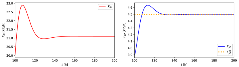
Figure 4: Setpoint tracking for $F_{pP}$ by proportional-integral control

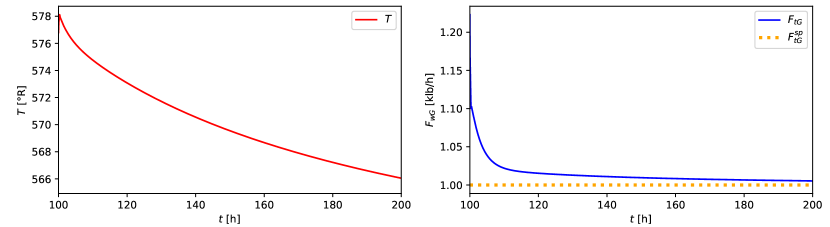
Figure 5: Setpoint tracking for $F_{wG}$ by proportional-integral control

5 Sample optimal control problems

Apart from setpoint tracking, another important task in process engineering is optimal control, that is, to optimize certain quality measures of a process by choosing optimally shaped control profiles. In our Williams-Otto example, typical quality measures are the total amount of waste and the total amount of product accumulated over the whole process duration. In general, the optimal control problems considered here read as follows:

$$\text{minimize or maximize }J(\bm{x},\bm{u})$$ (5.1)

($J$ being the desired process quality measure) subject to constraints of the form

$$\dot{\bm{x}}(t)=\bm{f}(\bm{x}(t),\bm{u}(t))\qquad(t\in[0,t_{f}])\qquad\text{and}\qquad\bm{x}(0)=\bm{x_{0}}$$ (5.2)

$$\bm{g}(\bm{x}(t),\bm{u}(t))\leq 0\qquad(t\in[0,t_{f}])$$ (5.3)

(differential-equation constraints and inequality constraints). It is easy to implement such optimal control problems in Pyomo. All one has to do is to complement the process equations (5.2) by the following specifications: one has to

• specify the goal function $J$ one wishes to minimize or maximize

• specify which control variables should be the free optimization variables and which shape the corresponding control profiles should have (general spline, piecewise constant, or constant)

• specify inequality constraints of the form (5.3) on the control and state variables, like box constraints on the controls or path constraints on state or output trajectories, for instance.

5.1 Waste minimization

In this subsection, we briefly discuss the waste minimization problem, that is, the goal function $J$ to be minimized is given by

$$J(\bm{x},\bm{u}):=\int_{0}^{t_{f}}F_{wG}(\tau)\,\mathrm{d}\tau,$$ (5.4)

where the waste stream $F_{wG}$ depends on $(\bm{x},\bm{u})$ according to (3.4) and (3.19) and where as total process time we choose $t_{f}=100$. As our free optimization variables we choose the feed stream $F_{fB}$ (profile type: piecewise constant) and the reactor temperature $T$ (profile type: general spline), as initial state $\bm{x_{0}}$ we choose the steady state (4.8), and as constraints we choose the following box constraints

$$F_{fA}=10,\quad 0\leq F_{fB}\leq 56,\quad 200\leq T\leq 800,\quad\mu=129.5,\quad\eta=0.2$$

After $257$ iterations and $16.7$ CPU seconds, the IPOPT solver then finds the control profiles from Figure 6 (top row) to be optimal (chosen number of finite elements and collocation points per finite element: $200$ and $3$, respectively). With these control profiles, the value of our total waste goal function is basically $0$ but, on the other hand, the total yield of our desired product is very small as well (Figure 6 (bottom row)). We therefore consider an appropriate yield maximization problem next.

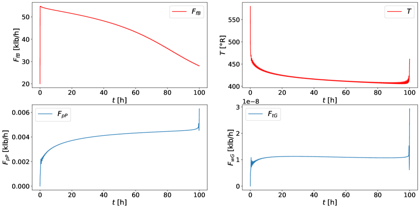
Figure 6: Control profiles minimizing the total waste (top row), and resulting stream profiles (bottom row)

5.2 Yield maximization

In this subsection, we discuss the yield maximization problem under a waste constraint, that is, the goal function $J$ to be maximized is given by

$$J(\bm{x},\bm{u}):=\int_{0}^{t_{f}}F_{pP}(\tau)\,\mathrm{d}\tau,$$ (5.5)

where the product stream $F_{pP}$ depends on $(\bm{x},\bm{u})$ according to (3.5) and (3.19) and where as total process time we choose $t_{f}=100$. As our free optimization variables we choose the feed stream $F_{fB}$ (profile type: general spline) and the reactor temperature $T$ (profile type: general spline), as initial state $\bm{x_{0}}$ we choose the steady state (4.8), and as constraints we choose the following box constraints

$$F_{fA}=10,\quad 0\leq F_{fB}\leq 56,\quad 200\leq T\leq 800,\quad\mu=129.5,\quad\eta=0.2$$

and, additionally, the following path constraint on the waste stream:

$$F_{wG}(t)\leq 1\qquad(t\in[0,t_{f}]).$$ (5.6)

After $1048$ iterations and $75.2$ CPU seconds, the IPOPT solver then finds the control profiles from Figure 7 (top row) to be optimal (chosen number of finite elements and collocation points per finite element: $200$ and $3$, respectively). With these control profiles, our yield goal function takes the value $611.3$. We see that the optimal $F_{fB}$-profile is bang-bang [11], [28] for a long period of time, that is, switching between the lower and upper bound for $F_{fB}$. Such a bang-bang behavior is not very popular in industrial practice as it can lead to an accelerated wear of the actuators. It is possible to reduce the bang-bang behavior of $F_{fB}$, without substantially decreasing the achieved yield value,

• by adding an appropriate upper-bound constraint on the integrated $F_{fB}$-control action $\int_{0}^{t_{f}}F_{fB}(\tau)\,\mathrm{d}\tau$ (hard constraint)

• or by adding the integrated $F_{fB}$-control action $\int_{0}^{t_{f}}F_{fB}(\tau)\,\mathrm{d}\tau$ with an appropriate weight to the original goal function (5.5) (soft constraint).

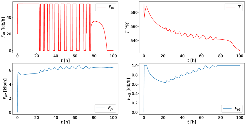
Figure 7: Control profiles maximizing the total yield under the waste constraint (5.6) (top row), and resulting stream profiles (bottom row)

We do not go into detail here because we achieved an even better bang-bang suppression (and, at the same time, even better total yield and total waste values) by the combined optimization approach presented next.

5.3 Combined waste and yield optimization

While in the previous two subsections we optimized waste and yield separately, we now want to optimize these conflicting quality measures simultaneously. In order to do so, we maximize the goal function $J$ given by

$$J(\bm{x},\bm{u}):=\alpha\int_{0}^{t_{f}}F_{pP}(\tau)\,\mathrm{d}\tau-\beta\int_{0}^{t_{f}}F_{wG}(\tau)\,\mathrm{d}\tau$$ (5.7)

with appropriately chosen weights $\alpha,\beta>0$. We choose the same final time $t_{f}$, the same initial state $\bm{x_{0}}$, and the same free optimization variables and constraints as in Section 5.1. Choosing equal weights $\alpha=1$ and $\beta=1$, we then find the control profiles from Figure 8 (top row) to be optimal after $388$ IPOPT iterations and $22.9$ CPU seconds (chosen number of finite elements and collocation points per finite element: $200$ and $3$, respectively). With these optimal control profiles, the yield is almost as large as in Section 5.2 (namely $608.3$ compared to $611.3$) while the total amount of waste is significantly smaller than in Section 5.2 (namely $56.5$ compared to $86.3$). A nice extra feature is that the strongly oscillatory bang-bang behavior in the optimal $F_{fB}$-profile from Section 5.2 is drastically reduced here.

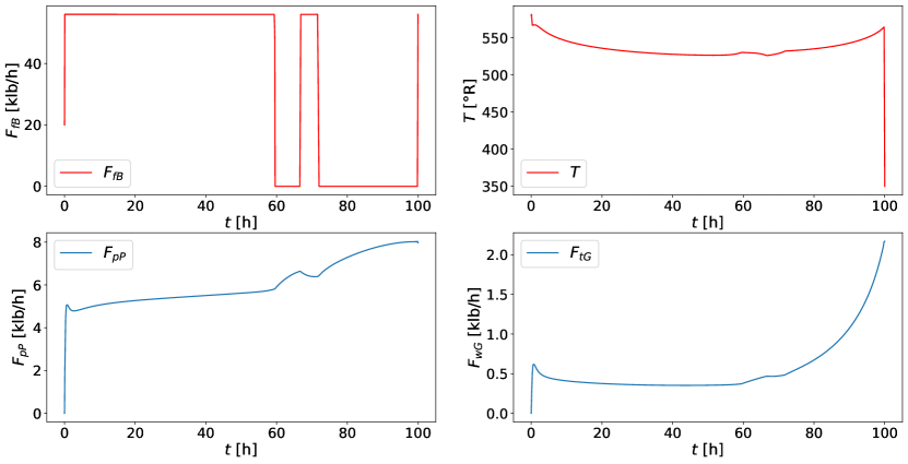
Figure 8: Control profiles maximizing the weighted sum (5.7) of total yield and total waste (top row), and resulting stream profiles (bottom row)

5.4 Setpoint tracking by means of optimal control

In the previous section, we discussed the standard approach to setpoint tracking based on feedback control, namely proportional-integral control. In this subsection, we present an alternative approach which is based on optimal control. In that approach, we formulate the setpoint tracking problem – which, recall, is about steering a process quantity $y$ to a steady-state setpoint $y^{sp}$ – as an optimal control problem (5.1)-(5.3) where the goal function $J$ is given by

$$J(\bm{x},\bm{u}):=\int_{t^{*}}^{t_{f}}(y(\tau)-y^{sp})^{2}\,\mathrm{d}\tau+\alpha\dot{\bm{x}}(t_{f})^{2}$$ (5.8)

and to be minimized. In this expression, $t^{*}$ is the time instant at which the user wants to start the setpoint tracking and $\alpha>0$ is a weight parameter. (As usual, the process should be in a steady state at this time $t^{*}$.) Clearly, by minimizing the first part of the goal function (5.8) we ensure that our setpoint quantity $y$ approaches its setpoint $y^{sp}$ as well and as quickly as possible, while by minimizing the second part of (5.8) we ensure that the process eventually is as close to a steady state as possible.

We apply this optimization-based approach of setpoint tracking to the same two examples as in the feedback-based approach before (Section 4.2), that is, as setpoint quantities we choose $F_{pP}$ and $F_{wG}$, respectively, and as corresponding optimal control variables we choose, respectively, $F_{fB}$ and $T$. Also, we choose the same time $t^{*}$ and the same initial state $\bm{x_{0}}$ and initial control profile $\bm{u}|_{[0,t^{*}]}\equiv\bm{u}^{*}$ as in Section 4.2. And finally, we choose $t_{f}=200$ and $\alpha=1$. Comparing the results (Figures 9 and 10) with our results from the feedback-based approach (Figures 4 and 5), we see that with the optimization-based approach the setpoints are reached much more quickly, namely within less than $10\%$ ($F_{pP}$ case) or $3\%$ ($F_{wG}$ case) of the time needed in the feedback-based approach.

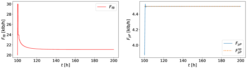
Figure 9: Setpoint tracking for $F_{pP}$ by optimal control

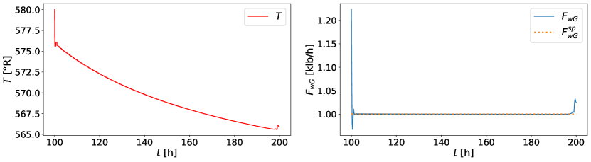
Figure 10: Setpoint tracking for $F_{wG}$ by optimal control

Additionally, the above optimization-based approach works just as well for tracking two setpoint quantities simultaneously, like $F_{pP}$ and $F_{wG}$ (instead of just a single one). In order to do so, one just has to use the vectorial setpoint quantity $\bm{y}:=(F_{pP},F_{wG})$ in (5.8) and minimize the resulting goal function w.r.t. the vectorial control quantity $(F_{fB},T)$. As has been remarked above (Section 4.2), the feedback-based approach, by contrast, has its limitations when applied to several control channels simultaneously.

6 Summary and discussion

In this paper, we dealt with the simulation and optimization of a prototypical process from chemical engenieering, the Williams-Otto process, using Pyomo, a powerful and versatile dynamic simulation and optimization software package based on Python. We discussed two typical optimal control problems for the Williams-Otto process, namely waste minimization and yield maximization. In order to set up and solve such optimal control problems in Pyomo, one basically only has to complement the dynamic process equations by the appropriate goal function and constraints. As one would expect, waste minimization and yield maximization are conflicting goals and we briefly discussed the combined optimization of these conflicting goals by a weighted-sum approach. In view of the non-convexity of the problem, it would be natural to further investigate this multicriteria optimization problem, however (Pareto front approximation and navigation  [29], [9], [12], for instance). A first study in that direction, for the reactor subsystem of the Williams-Otto process, is undertaken in [23]. Aside from process optimization, we also discussed two approaches to the setpoint tracking problem:

• one standard approach which is based on feedback control, more precisely, on proportional-integral control, and

• one approach that is based on optimal control.

We saw that with the optimization-based approach, setpoints are typically reached more quickly and more reliably. In order to perform setpoint tracking in Pyomo by means of proportional-integral control, one basically only has to complement the dynamic process equations by the appropriate feedback relations. It would be natural and interesting to further investigate setpoint tracking using yet another approach, namely model-predictive control [1], [18], [16], [3] which combines the feedback- and optimization-based approaches from above. Just like the two approaches disscussed above, a model-predictive control scheme for the Williams-Otto process could be implemented in a quite straightforward manner with Pyomo. (See [2] for a discussion of model-predictive control for the reactor subsystem of the Williams-Otto process.)

7 Conclusion

In this paper, we illustrated the advantages that a high-level software package (Pyomo) can provide for the chemical engineer. We paradigmatically solved a number of increasingly complex dynamic simulation and optimization problems based on the Williams-Otto process. We performed waste and yield optimization. Additionally, we contrasted the use of proportional-integral controllers with an open-loop optimization approach for setpoint tracking.

References

- [1] F. Allgöwer, A. Zheng (editors): Nonlinear model-predictive control. Birkhäuser (2000)
- [2] R. Amrit: Optimizing process economics in model-predictive control. Ph.D. thesis, University of Wisconsin, Madison (2011)
- [3] J.A.E. Andersson, J. Gillis, G. Horn, J.B. Rawlings, M. Diehl: CasADi: a software framework for nonlinear optimization and optimal control. Math. Prog. Comp. 11 (2019), 1–36
- [4] F. Assassa, W. Marquardt: Dynamic optimization using adaptive direct multiple shooting. Comp. Chem. Eng. 60 (2014), 242-259
- [5] T. Bhatia, L. T. Biegler: Dynamic optimization in the design and scheduling of multiproduct batch plants. Ind. Eng. Chem. Res. 35 (1996), 2234
- [6] L.T. Biegler: Nonlinear programming. Concepts, algorithms, and applications to chemical processes. MOS-SIAM Series on Optimization (2010)
- [7] L.T. Biegler, I.E. Grossmann, A.W. Westerberg: Systematic methods of chemical process design. Prentice Hall (1997)
- [8] H.G. Bock, K.J. Plitt: A multiple shooting algorithm for direct solution of optimal control problems. IFAC Proceedings Volumes 17 (1984), 1603-1608
- [9] M. Bortz, J. Burger, N. Asprion, S. Blagov, R. Böttcher, U. Nowak, A. Scheithauer, R. Welke, K.-H. Küfer, H. Hasse: Multi-criteria optimization in chemical process design and decision support by navigation on Pareto sets. Comp. Chem. Eng. 60 (2014), 354-363
- [10] M. Bortz, R. Heese, A. Scherrer, T. Gerlach, T. Runowski: Estimating mixture properties from batch distillation using semi-rigorous and rigorous models. In A.A. Kiss, E. Zondervan, R. Lakerveld, L. Özkan (editors): Proceedings of the 29th European Symposium on Computer Aided Process Engineering. Elsevier (2019)
- [11] A. Bressan, B. Piccoli: Introduction to the mathematical theory of control. AIMS Series on Applied Mathematics (2007)
- [12] J. Burger, N. Asprion, S. Blagov, R. Böttcher, U. Nowak, M. Bortz, R. Welke, K.-H. Küfer, H. Hasse: Multi-objective optimization and decision support in process engineering – Implementation and application. Chem. Ing. Techn. 86 (2014), 1065-1072
- [13] A. Oliveira Cardoso, W.H. Kwong: Williams-Otto plant control based on production planning associated to coordinated decentralized optimization and plantwide control techniques. J. Chem. Chem. Eng. 10 (2016), 77-89
- [14] A. Cervantes, L.T. Biegler: Large-scale DAE optimization using simultaneous nonlinear programming formulations. AIChE J. 44 (1998), 1038
- [15] M. Diehl, H.G. Bock, H. Diedam, P.-B. Wieber: Fast direct multiple shooting algorithms for optimal robot control. In: Fast motions in biomechanics and robotics, Lecture Notes in Control and Information Sciences 340 (2006), 65-93
- [16] R. Findeisen, F. Allgöwer, L.T. Biegler (editors): Assessment and future directions of nonlinear model predictive control. Springer (2007)
- [17] M. Grötschel, S. Krumke, J. Rambau (editors): Online optimization of large systems. Springer (2001)
- [18] L. Grüne, J. Pannek: Nonlinear model predictive control. Theory and algorithms. 2nd edition, Springer (2017)
- [19] R. Hannemann-Tamas, W. Marquardt: How to verify optimal controls computed by direct shooting methods? – A tutorial. J. Proc. Contr. 22 (2012), 494-507
- [20] W.E. Hart, J.-P. Watson, D.L. Woodruff: Pyomo: modeling and solving mathematical programs in Python. Math. Program. Comp. 3 (2011), 219-260
- [21] W.E. Hart, C.D. Laird, J.-P. Watson, D.L. Woodruff, G.A. Hackebeil, B.L. Nicholson, J.D. Siirola: Pyomo – Optimization modeling in Python. 2nd edition, Springer (2017)
- [22] B. Houska, H.J. Ferreau, M. Diehl: ACADO toolkit – An open-source framework for automatic control and dynamic optimization. Optim. Control Appl. Meth. 32 (2011), 298–312
- [23] F. Logist, M. Vallerio, B. Houska, M. Diehl, J. Van Impe: Multi-objective optimal control of chemical processes using ACADO toolkit. Comp. Chem. Eng. 37 (2012), 191-199
- [24] B.L. Nicholson, J.D. Siirola, J.-P. Watson, V.M. Zavala, L.T. Biegler: pyomo.dae: a modeling and automatic discretization framework for optimization with differential and algebraic equations. Math. Progr. Comp. 10 (2018), 187–223
- [25] A. O’Dwyer: An overview of tuning rules for the PI and PID continuous-time control of time-delayed single-input, single-output (SISO) processes. In R. Vilanova, A. Visioli: PID control in the third millennium, Springer (2012)
- [26] S. Skogestad: Tuning for smooth PID control with acceptable disturbance rejection. Ind. Eng. Chem. Res. 45 (2006), 7817–7822
- [27] S. Skogestad, C. Grimholt: The SIMC method for smooth PID controller tuning. In R. Vilanova, A. Visioli: PID control in the third millennium, Springer (2012)
- [28] E.D. Sontag: Mathematical control theory. Deterministic finite-dimensional systems. 2nd edition, Springer (1998)
- [29] K. Teichert: A hyperboxing Pareto approximation method applied to radiofrequency ablation treatment planning. Ph.D. thesis, Technical University of Kaiserslautern (2014)
- [30] I.-B. Tjoa, L.T. Biegler: Simultaneous solution and optimization strategies for parameter estimation of differential-algebraic equation systems. Ind. Eng. Chem. Res. 30 (1991), 376–385
- [31] R. Vilanova, A. Visioli: PID control in the third millennium. Springer (2012)
- [32] A. Wächter, L.T. Biegler: Line Search Filter Methods for Nonlinear Programming: Motivation and Global Convergence. SIAM J. Optim. 16 (2005), 1–31
- [33] A. Wächter, L.T. Biegler: Line Search Filter Methods for Nonlinear Programming: Local Convergence. SIAM J. Optim. 16 (2005), 32-48
- [34] A. Wächter, L.T. Biegler: On the implementation of an interior-point filter line-search algorithm for large-scale nonlinear programming. Math. Progr. 106 (2006), 25–57
- [35] T. Williams, R. Otto: A generalized chemical processing model for the investigation of computer control. AIEE Trans. 79 (1960), 458-473