Inference by Stochastic Optimization:
A Free-Lunch Bootstrap

Abstract

Assessing sampling uncertainty in extremum estimation can be challenging when the asymptotic variance is not analytically tractable. Bootstrap inference offers a feasible solution but can be computationally costly especially when the model is complex. This paper uses iterates of a specially designed stochastic optimization algorithm as draws from which both point estimates and bootstrap standard errors can be computed in a single run. The draws are generated by the gradient and Hessian computed from batches of data that are resampled at each iteration. We show that these draws yield consistent estimates and asymptotically valid frequentist inference for a large class of regular problems. The algorithm provides accurate standard errors in simulation examples and empirical applications at low computational costs. The draws from the algorithm also provide a convenient way to detect data irregularities.

JEL Classification: C2, C3

Keywords: Stochastic gradient descent, Newton-Raphson, Simulation-Based Estimation.

1 Introduction

Many questions of economic interest can be expressed as non-linear functions of unknown parameters $\theta$ that need to be estimated from a sample of data of size $n$. The typical econometric routine is to first obtain a consistent estimate $\hat{\theta}_{n}$ of the true value $\theta^{0}$ by minimizing an objective function $Q_{n}(\theta)$, after which its sampling uncertainty is assessed. Though gradient-free optimizers provide point estimates, its asymptotic variance is often analytically intractable. One remedy is to use bootstrap standard errors, but this requires solving the minimization problem each time the data is resampled, and for complex models, this is no simple task. There is a long-standing interest in finding ‘short-cuts’ that can relieve the computation burden without sacrificing too much accuracy. Examples include Davidson and MacKinnon (1999), Andrews (2002), Kline and Santos (2012), Armstrong et al. (2014) and more recently Honoré and Hu (2017). These methods provide standard errors by taking a converged estimate $\hat{\theta}_{n}$ as given. As such, estimation always precedes inference.

This paper proposes a resampling scheme that will deliver both the point estimates of $\theta$ and its standard errors within the same optimization framework. Since the standard errors are obtained as a by-product of point estimation, we refer to the procedure as a ‘free-lunch bootstrap’. The free-lunch is made possible by a specially designed stochastic optimization algorithm that resamples batches of data of size $m\leq n$. Given an initial guess $\theta_{0}$, one updates $\theta_{b}$ for $b\geq 0$ to $\theta_{b+1}$ using the gradient, the inverse Hessian as conditioning matrix, and a suitably chosen learning rate. We first show that the average over $B$ draws of $\theta_{b}$ is equivalent to the mode $\hat{\theta}_{n}$ obtained by classical optimization up to order $\frac{1}{m}$. We then show that the distribution of $\sqrt{m}(\theta_{b}-\hat{\theta}_{n})$ conditional on the original sample of data is first-order equivalent to that of $\sqrt{n}(\hat{\theta}_{n}-\theta^{0})$ upon rescaling, making it a bootstrap distribution. Because the conditioning matrix is the inverse Hessian, the procedure is a resampled Newton-Raphson (rnr) algorithm. For other conditioning matrices, the draws from resampling still produce a consistent estimate but cannot be used for inference.

The main appeal of the proposed methodology is its simplicity. If the optimization problem can be solved by our stochastic optimizer, inference can be made immediately without further computations. Natural applications include two-step estimation when the parameters in the two steps are functionally dependent in a complicated way, as well as minimum distance estimation that compares the empirical moments with the model moments expressed as a function of the parameters. When such a mapping cannot be expressed in closed-form, simulation estimation makes progress by using Monte-Carlo methods to approximate the binding function, but computing standard errors of the simulation-based estimates remains a daunting task. Our algorithm provides an automated solution to compute standard errors and removes simulation noise, resulting in more accurate estimates. The algorithm also provides a convenient way to compute clustered standard errors and model diagnostics.

As compared to other stochastic optimization algorithms, we use a learning rate that is fixed rather than vanishing, and though a small $m$ is desirable from a pure computation perspective, valid inference necessitates that $m$ cannot be too small. As compared to conventional bootstrap methods, the simultaneous nature of estimation and inference means that a preliminary $\hat{\theta}_{n}$ is not needed for resampling. Though $\theta_{b}$ is a Markov chain, no prior distribution is required, nor are Bayesian computation tools employed. In simulated examples and applications, our bootstrap standard errors match up well with the asymptotic and bootstrap analogs, but at significantly lower computational costs.

The plan of the paper is as follows. Section 2 begins with a review of classical and stochastic optimization. The proposed free-lunch algorithm is presented in Section 3 and its relation to other resampling procedures is explained. The properties of the draws from the algorithm are derived in Section 4. Simulated and empirical examples are presented in Section 5. Section 6 extends the main results to simulation-based estimation. Appendix A provides derivations of the main results. An on-line supplement provides the r code to implement one of the applications considered, additional results with details for replications, as well as an analytical example for Section 6.

2 Review of the Related Literature

Consider minimization of the objective function $Q_{n}(\theta)$ with respect to $\theta$ whose true value is $\theta^{0}$. The sample gradient and Hessian of $Q_{n}(\theta)$ are defined respectively by

$$G_{n}(\theta) = \nabla Q_{n}(\theta;x)=\frac{1}{n}\sum_{i=1}^{n}\nabla Q_{n}(\theta;x_{i})$$

$$H_{n}(\theta) = \nabla^{2}Q_{n}(\theta;x)=\frac{1}{n}\sum_{i=1}^{n}\nabla^{2}Q_{n}(\theta;x_{i}).$$

The necessary conditions for a local minimum are $\|G_{n}(\hat{\theta}_{n})\|=0$ and $H_{n}(\hat{\theta}_{n})$ positive semi-definite. The sufficient conditions are $\|G_{n}(\hat{\theta}_{n})\|=0$ and $H_{n}(\hat{\theta}_{n})$ positive definite. To find the optimal solution, a generic rule for updating from the current estimate $\theta_{k}$ is

$$\theta_{k+1}=\theta_{k}-\gamma_{k}Z_{n}(\theta_{k})$$

where $\gamma_{k}$ is the step size and $Z_{n}=\frac{\partial\theta_{k+1}}{\partial\gamma_{k}}$ is the direction of change.

Gradient based methods specify $Z_{n}(\theta_{k})=P_{n}(\theta_{k})G_{n}(\theta_{k})$ where $P_{n}(\theta_{n})$ is a conditioning matrix. The updating rule then becomes

$$\theta_{k+1} \equiv \theta_{k}-\gamma_{k}P_{n}(\theta_{k})G_{n}(\theta_{k}).$$ (1)

The method of gradient descent (gd) (also known as steepest descent) sets $P_{n}=I_{d}$. Since gd does not involve the Hessian, it is a first order method and is less costly. Convergence of $\hat{\theta}_{k}$ to the minimizer $\hat{\theta}_{n}$ is linear under certain conditions, but the rate depends on $I_{d}-\gamma H_{n}(\theta_{k})$ being in the restricted region of $(-1,1)$, and can be slow when the ratio of the maximum to the minimum eigenvalue of $H_{n}$ is large. The Newton-Raphson algorithm puts $P_{n}=H_{n}(\theta_{k})^{-1}$. It is a second-order method since it involves the Hessian matrix. When $\gamma_{k}=1$, the algorithm converges quadratically if $Q_{n}$ satisfies certain conditions. A drawback of Newton’s algorithm is that it requires computation of the inverse of the Hessian. When strong convexity fails, the Hessian could be non-positive definite for $\theta$ away from the minimum. In such cases, it is not uncommon to replace the Hessian by $H_{n}(\theta_{k})+c\cdot I_{d}$ for some $c>0$, or specify $P_{n}=(H_{n}(\theta_{k})^{\prime}H_{n}(\theta_{k}))^{1/2}$ to restore positive definiteness around saddle-points, see Nocedal and Wright (2006, Chapter 3.4). Quasi-Newton methods bypass direct computation of the Hessian or its inverse, but analytical convergence results are more difficult to obtain. We focus our theoretical analysis on gradient descent and Newton-Raphson based algorithms but will consider quasi-Newton methods in some simulations.

2.1 Stochastic Optimization

Stochastic optimization finds the optima in noisy observations using carefully designed recursive algorithms. The idea can be traced to the theory of stochastic approximation when the goal is to minimize some function $Q(\theta)$ with gradient $G(\theta)$, which is equivalent to the root-finding problem $G(\theta)=0$ whose the true value is $\theta^{0}$. A classical optimizer would perform $\theta_{k+1}=\theta_{k}-\gamma_{k}G(\theta_{k})$. Robbins and Monro (1951) considers the situation when we only observe $G(\theta_{k})+e_{k}$ with $\mathbb{E}(e_{k})=0$ and suggests to update according to

$$\theta_{k+1}=\theta_{k}-\gamma_{k}(G(\theta_{k})+e_{k}).$$

Robbins and Monro (1951) proved that $\theta_{k}\smash{\mathop{\longrightarrow}\limits^{as}}\theta^{0}$ for $G$ non-decreasing with step size sequence $\gamma_{k}\geq 0$ satisfying

$$\text{(i)}\quad\sum_{k=1}^{\infty}\gamma_{k}=+\infty,\quad\quad\text{(ii)}\quad\sum_{k=1}^{\infty}\gamma_{k}^{2}<+\infty.$$ (2)

The first condition ensures that all possible solutions will be reached with high probability regardless of the starting value, while the second ensures convergence to the true value. Building on the Robbins-Monro algorithm, the Kiefer-Wolfowitz algorithm uses a finite difference approximation $G(\theta_{k})\approx G_{n}(\theta_{k})=\frac{1}{2\epsilon_{k}}\bigg{[}Q_{n}(\theta_{k}+\epsilon_{k})-Q_{n}(\theta_{k}-\epsilon_{k})\bigg{]}$. This is often recognized as the first implementation of stochastic gradient descent. Kiefer and Wolfowitz (1952) proves convergence of $\theta_{k}$ to the maxiumum likelihood estimate $\hat{\theta}_{n}$ assuming that the likelihood $Q_{n}$ is convex, $\epsilon_{k}$ goes to zero, and that the two conditions stated in (2) hold.

Modern stochastic gradient descent updates according to

$$\theta_{k+1} = \theta_{k}-\gamma_{k}G_{m}(\theta_{k})$$

where $G_{m}(\theta_{k})=\frac{1}{m}\sum_{i=1}^{m}G(\theta_{k};x_{i})$ is an estimate of $G(\theta)$. It can be seen as Monte-Carlo based since the $m$ observations used to compute $G_{m}(\theta_{k})$ are usually chosen from $\{1,\dots,n\}$ randomly. Though $m=1$ is computationally inexpensive and is a popular choice, a small $\gamma_{k}$ is often needed to compensate for the higher variation. A common rule is to choose $\gamma_{k}=\gamma k^{-\delta}$, where $\delta\in(1/2,1]$ and $\gamma>0$ are the choice parameters. Depending on $\delta$, convergence as measured by $\mathbb{E}(\|\theta_{k}-\theta^{0}\|^{2})$ can occur at a $1/k$ rate or slower. To reduce sensitivity to the tuning parameters, Ruppert (1988) and Polyak and Juditsky (1992) propose to accelerate convergence using what is now known as Polyak-Ruppert averaging: $\overline{\theta}_{k}=\frac{1}{k}\sum_{i=1}^{k}\theta_{i}$. Importantly, $\overline{\theta}_{k}$ converges at the fastest $1/k$ rate for all choices of $\delta\in(1/2,1]$. Moulines and Bach (2011) shows that the improvements hold even for a finite number of iterations $k$. We will return to Polyak-Ruppert averaging below.

Stochastic optimization presents an interesting alternative to classical optimization as it approximates the gradient on minibatches of the original data. This is particularly helpful in large scale learning problems such Lasso, support-vector machines and K-means clustering when non-linear optimization can be challenging. Improvements to sgd with $P_{m}=I_{d}$ include momentum (Polyak, 1964) and accelerated gradient (Nesterov, 1983) methods. Besides its computational appeal, stochastic optimization can improve upon its classical counterpart in non-convex settings.

A variation of sgd, known as Stochastic gradient Langevin dynamics (sgld) incorporates Langevin dynamics into a Bayesian sampler. As will be discussed further below, the update is based on the gradient of the posterior distribution. Of note now is that sgld has two types of noises: an injected noise, and the stochastic gradient noise based on $m\ll n$ observations. They play different roles in the algorithm. In the early phase of sgld, the stochastic gradient dominates and the algorithm performs optimization. In the second phase, the injected noise dominates and the algorithm behaves like a posterior sampler. The algorithm seamlessly switches from one phase to another for an appropriate choice of the learning rate.

Unlike classical optimization, stochastic Newton-Raphson with the inverse Hessian $H_{m}(\theta)$ as conditioning matrix is not popular because the Hessian is often noisy and near singular for $m$ small, rendering the algorithm unstable. We will show that using a variation of stochastic Newton-Raphson with larger batches of data can produce draws that not only provide an accurate estimate of $\theta^{0}$ but also yields frequentist assessment of sampling uncertainty. It thus integrates numerical optimization with statistical inference. In contrast, other conditioning matrices will yield consistent estimates but would not provide valid inference in our setup.

3 Extremum Estimation and Inference by Resampling

Consider extremum estimation of parameters $\theta\in\Theta\subset\mathbb{R}^{d}$ from data $x=(x_{1},\ldots,x_{n})$. Let $\theta^{0}$ be the minimizer of a twice differentiable population objective function $Q(\theta)$ whose sample analog is $Q_{n}(\theta)\equiv Q_{n}(\theta;x)$. The sample extremum estimator is

$$\hat{\theta}_{n}=\text{argmin}_{\theta\in\Theta}Q_{n}(\theta).$$

For likelihood estimation, $Q_{n}(\theta)=-\sum_{i=1}^{n}\ell_{i}(\theta)$ where $\ell_{i}$ is the likelihood of $\theta$ at observation $x_{i}$. For least squares estimation, $Q_{n}(\theta)$ is the sum of squared residuals $\sum_{i=1}^{n}e_{i}^{2}(\theta)$. For GMM estimate with positive weighting matrix $W_{n}$, $Q_{n}(\theta)=\overline{g}_{n}(\theta)^{\prime}W_{n}\overline{g}_{n}(\theta)$ where $\mathbb{E}[g_{i}(\theta^{0})]=0$. Under regularity conditions stated in Theorem 2.1 of Newey and McFadden (1994) $\hat{\theta}_{n}$ is consistent for $\theta^{0}$. If, in addition, the assumptions in Theorem 3.1 of Newey and McFadden (1994) hold, then $\hat{\theta}_{n}$ is also $\sqrt{n}$-asymptotically normal:

$$\sqrt{n}(\mathbb{V}^{0})^{-1/2}(\hat{\theta}_{n}-\theta^{0})\smash{\mathop{\longrightarrow}\limits^{d}}N(0,I_{d})$$

where $\mathbb{V}^{0}=[H(\theta^{0})]^{-1}\text{var}(\sqrt{n}G_{n}(\theta^{0}))[H(\theta^{0})]^{-1}$. Finite sample inference is typically based on an estimate of $\mathbb{V}^{0}$ which can be analytically intractable or costly to compute on the full sample. It is not uncommon to resort to bootstrap inference. We consider the $m$ out of $n$ bootstrap with $m\to\infty,m/n\to c\in[0,1]$ and samples $(x_{1}^{(b)},\dots,x_{m}^{(b)})$ with replacement from the data $(x_{1},\dots,x_{n})$ for $b=1,\dots,B$ and solve $B$ minimization problems:

$$\hat{\theta}_{m}^{(b)}=\text{argmin}_{\theta\in\Theta}Q_{m}^{(b)}(\theta),$$

where the resampled objective $Q_{m}^{(b)}(\theta)=Q_{m}^{(b)}(\theta,x^{(b)})$ is computed over the sample $x^{(b)}$.

Let $\mathbb{E}^{\star}$ and $\text{var}^{\star}$ denote the bootstrap expectation and variance which are taken conditional on the sample data $(x_{1},\dots,x_{n})$, and $\overset{d^{\star}}{\to}$ denotes the convergence in distribution conditional on the data. Since we only consider correctly specified regular estimators, the desired convergence is to a Gaussian limit. The $m$ out of $n$ bootstrap can allow for different sampling schemes. Assuming that the resampling scheme is chosen to reflect the dependence structure of the data, it holds in a variety of settings that

$$\sqrt{m}(\mathbb{V}_{m})^{-1/2}\left(\hat{\theta}_{m}^{(b)}-\hat{\theta}_{n}\right)\overset{d^{\star}}{\to}\mathcal{N}\left(0,I_{d}\right),$$

where $\mathbb{V}_{m}=[H_{n}(\hat{\theta}_{n})]^{-1}\text{var}^{\star}(\sqrt{m}G_{m}^{(b)}(\hat{\theta}_{n}))[H_{n}(\hat{\theta}_{n})]^{-1}$ depends on the inverse Hessian as well as the variance of the resampled score. The result implies that the resampled distribution of $\hat{\theta}_{m}^{(b)}$ can be used to approximate the sampling distribution of $\hat{\theta}_{n}$.

An $m$ out of $n$ bootstrap with $m<n$ uses smaller samples and performs as well as a $n$ out of $n$ bootstrap in simulations while requiring similar or weaker conditions, (Bickel et al., 2012). Nonetheless, it still makes multiple calls to a classical optimizer. As will be seen below, our proposed algorithm only requires one call to the optimizer.

We propose the following two algorithms and use ‘$b$’ to index the iterates of the algorithm. In this notation, $G_{m}^{(b+1)}(\theta_{b})$ is the gradient computed on the $(b+1)$-th batch of resampled data of size $m$ and evaluated at $\theta_{b}$, the parameter value in the previous draw, and $H_{m}^{(b+1)}(\theta_{b})$ is similarly defined.

Algorithm 1 Estimation by Resampling

Input: (a) an initial guess $\theta_{0}$, (b) a bootstrap sample size $B$ and a burn-in period burn, (c) a batch size $m\leq n$, (d) a fixed learning rate $\gamma\in(0,1]$, (e) a conditioning matrix $P_{b}$

Burn-in and Resample:

for $b=1,\dots,\textsc{burn}+B$ do

     Resample the $(b+1)$-th batch of data of size $m$

     Update $P_{b}$ and $G_{b}=G_{m}^{(b+1)}(\theta_{b})$.

     Update $\theta_{b+1}=\theta_{b}-\gamma P_{b}G_{b},$

end for

Discard the first burn draws, re-index $\theta_{\text{burn}+b}$ to $\theta_{b}$ for $b=1,\ldots B$.

Let $\overline{\theta}_{\textsc{re}}=\frac{1}{B}\sum_{b=1}^{B}\theta_{b}$.

Algorithm 2 The Free-Lunch Bootstrap

Implement Algorithm 1 with $P_{b}=H_{b}^{-1}$.

Let $\overline{\theta}_{r\textsc{nr}}=\frac{1}{B}\sum_{b=1}^{B}\theta_{b}$ and define $\widehat{\text{var}}(\theta_{b})=\frac{1}{B}\sum_{b=1}^{B}(\theta_{b}-\overline{\theta}_{r\textsc{nr}})(\theta_{b}-\overline{\theta}_{r\textsc{nr}})^{\prime}.$

Output: $\overline{\theta}_{r\textsc{nr}}$ and $V_{r\textsc{nr}}=\frac{m}{\phi(\gamma)}\widehat{\text{var}}(\theta_{b})$, where $\phi(\gamma)=\frac{\gamma^{2}}{1-(1-\gamma)^{2}}$.

Algorithm 1 produces an estimate $\overline{\theta}_{\textsc{re}}$ by resampling, hence the acronym re. It works for any conditioning matrix $P_{b}$ satisfying assumptions to be made precise in Theorem 1. Algorithm 2 produces draws using the inverse Hessian as $P_{b}$ as in Newton-Raphson, hence the acronym rnr. The free-lunch aspect relates to the fact that we get both an estimate $\overline{\theta}_{r\textsc{nr}}$ and its standard error in one run. The bootstrap aspect comes from the fact that under the assumptions of Theorem 2, $\sqrt{m}(\theta_{b}-\hat{\theta}_{n})$ has the same asymptotic distribution as $\sqrt{n}(\hat{\theta}_{n}-\theta^{0})$ after an adjustment of $\frac{m}{\phi(\gamma)}$. The quantity $V_{r\textsc{nr}}$ is an estimate of the sandwich variance that is computationally costly for classical estimation. A Wald test for $H_{0}:\theta=\theta^{\dagger}$ can be constructed as

$$\text{wald}=n(\overline{\theta}_{r\textsc{nr}}-\theta^{\dagger})^{\prime}V_{r\textsc{nr}}^{-1}(\overline{\theta}_{r\textsc{nr}}-\theta^{\dagger})$$

which has an asymptotic Chi-squared distribution under the null hypothesis. A 95% level bootstrap confidence interval can also be constructed after adjusting for $\frac{m}{n}$ and $\phi(\gamma)$ by taking the (0.025,0.975) quantiles of $\big{\{}\overline{\theta}_{r\textsc{nr}}+\sqrt{\frac{m}{n\phi(\gamma)}}(\theta_{b}-\overline{\theta}_{r\textsc{nr}})\big{\}}_{b\geq 1}$.

Algorithms 1 and 2 have three features that distinguish them from existing gradient-based stochastic optimizers. First, $\gamma\in(0,1]$ does not change with $b$. Fixing $\gamma$ rather than letting $\gamma_{b}\rightarrow 0$ potentially permits faster convergence. Second, we sample $m$ out of $n$ observations with $m/n\rightarrow c\in[0,1]$ and $\sqrt{n}/m\to 0$. This precludes the popular choice in stochastic optimization of $m=1$, but admits $m=n$. We thus accept a higher computation cost to accommodate inference. Third, compared to sgd  Algorithm 2 uses the inverse Hessian as conditioning matrix.

3.1 The Linear Regression Model

This subsection uses the linear regression model to gain intuition of the Free-Lunch bootstrap. The model is $y_{i}=x_{i}^{\prime}\theta+e_{i}$. Let $\hat{e}_{n}=y_{n}-X_{n}\hat{\theta}_{n}$ be the $n\times 1$ vector of least squares residuals evaluated at the solution $\hat{\theta}_{n}$. $X_{n}$ denote the $n\times K$ matrix of regressors. The linear model is of interest because the objective function is quadratic and the quantities required for updating are analytically tractable. The gradient and Hessian of the full sample objective function $Q_{n}(\theta)=(y_{n}-X_{n}\theta)^{\prime}(y_{n}-X_{n}\theta)/(2n)$ are $G_{n}(\theta)=-X_{n}^{\prime}(y_{n}-X_{n}\theta)/n$ and $H_{n}(\theta)=X_{n}^{\prime}X_{n}/n$. The updates for this linear model evolve as

$$\theta_{k+1} = \theta_{k}+\gamma P_{k}X_{n}^{\prime}(y_{n}-X_{n}\theta_{k})/n$$

$$= \theta_{k}+\gamma P_{k}X_{n}^{\prime}\bigg{(}X_{n}(\hat{\theta}_{n}-\theta_{k})+\hat{e}_{n}\bigg{)}/n.$$

Convergence of $\theta_{k}$ for a given conditioning matrix $P_{k}$ can be studied by subtracting $\hat{\theta}_{n}$ from both sides of the updating equation and re-arranging terms (see Appendix A.1 for details). Table 1 summarizes convergence of gd, nr, sgd, rgd  and rnr. snr  is not considered because $X_{m}^{\prime}X_{m}/m$ is singular for $m=1$ so $\theta_{b}$ is not well defined. The left panel of the table gives the updating rule in closed form and the right panel expresses the deviation of the draws from $\hat{\theta}_{n}$ as the sum of a deterministic and a stochastic component.

Table 1: OLS: updating rules and convergence

Method	Conditioning	Update:	Convergence: $\theta_{k+1}-\hat{\theta}_{n}$=
	Matrix $P_{k}$	$\theta_{k+1}-\theta_{k}=$	deterministic	+	stochastic
gd	$I_{d}$	$-\gamma_{k}G_{k}$	$(I_{d}-\gamma H_{n})(\theta_{k}-\hat{\theta}_{n})$
sgd	$I_{d}$	$-\gamma_{b}G_{b}$	$(I_{d}-\gamma_{b}H_{b})(\theta_{b}-\hat{\theta}_{n})$	$-$	$\gamma_{b}G_{b}(\hat{\theta}_{n})$
rgd	$I_{d}$	$-\gamma G_{b}$	$(I_{d}-\gamma H_{b})(\theta_{b}-\hat{\theta}_{n})$	$+$	$\gamma H_{b}(\hat{\theta}_{m}^{(b+1)}-\hat{\theta}_{n})$
nr	$H_{k}^{-1}$	$-\gamma H_{k}^{-1}G_{k}$	$(1-\gamma)(\theta_{k}-\hat{\theta}_{n})$
rnr	$H_{b}^{-1}$	$-\gamma H_{b}^{-1}G_{b}$	$(1-\gamma)(\theta_{b}-\hat{\theta}_{n})$	$+$	$\gamma(\hat{\theta}_{m}^{(b+1)}-\hat{\theta}_{n})$

Note: $G_{k}=G_{n}^{(k+1)}(\theta_{k})$, $G_{b}=G_{m}^{(b+1)}(\theta_{b})$, $H_{k}=H_{n}^{(k+1)}(\theta_{k})$, $H_{b}=H_{m}^{(b+1)}(\theta_{b})$.

As seen from Table 1, gd updates do not depend on the Hessian but convergence does, while for nr  the opposite is true. Convergence of nr  can be achieved after one iteration if $\gamma=1$. In sgd, rgd  and rnr, batch resampling adds a stochastic component to the updates and convergence is no longer deterministic. The deviations for sgd  and rgd  $\theta_{b+1}-\hat{\theta}_{n}$ follow a VAR(1) process with varying and fixed coefficient matrices $I_{d}-\gamma_{b}H_{b}$ and $I_{d}-\gamma H_{b}$, respectively. In contrast, the rnr draws have an AR(1) representation with a fixed coefficient $(1-\gamma)$ that is dimension-free and independent of the Hessian. Note that rgd  and rnr  keep $\gamma$ fixed and rely on averaging over $b$ for convergence.

Our main result pertains to rnr  so it is useful to have a deeper understanding of how it works. Unlike stochastic optimizers which require $\gamma_{b}$ vanishing, the learning rate $\gamma$ used to generate the rnr  draws is constant. The draws evolve according to

$$\theta_{b+1}-\hat{\theta}_{n}=(1-\gamma)(\theta_{b}-\hat{\theta}_{n})+\gamma(\hat{\theta}^{(b+1)}_{m}-\hat{\theta}_{n})$$ (3)

where $\hat{\theta}_{m}^{(b+1)}=(X_{m}^{(b+1)\prime}X_{m}^{(b+1)})^{-1}X_{m}^{(b+1)\prime}y_{m}^{(b+1)}$ is obtained by classical optimization using the $(b+1)$-th bootstrap sample $(y_{i}^{(b+1)},x_{i}^{(b+1)})_{i=1,\dots,m}$. Being a bootstrap estimate, it holds under regularity conditions that the distribution of $\sqrt{m}(\hat{\theta}_{m}^{(b+1)}-\hat{\theta}_{n})$ conditional on the data approximates the sampling distribution of $\sqrt{n}(\hat{\theta}_{n}-\theta^{0})\smash{\mathop{\longrightarrow}\limits^{d}}N(0,\mathbb{V}^{0})$.

Clearly when $\gamma=1$, (3) implies $\theta_{b}=\hat{\theta}_{m}^{(b)}$, meaning that each rnr  draw equals the bootstrap estimate $\hat{\theta}_{m}^{(b)}$. We want to show that the draws are still bootstrap estimates when $\gamma\in(0,1)$. For such $\gamma$, $\theta_{b+1}-\hat{\theta}_{n}$ is an AR(1) process where for each $b$, the innovations $\gamma(\hat{\theta}_{m}^{(b+1)}-\hat{\theta}_{n})$ are iid conditional on the original sample. Iterating the AR(1) formula backwards to the initial value $\theta_{0}$, we can decompose the draws $\theta_{b+1}$ into two terms:

$$\theta_{b+1}-\hat{\theta}_{n}=\underbrace{\vphantom{\gamma\sum_{j=0}^{b}(1-\gamma)^{j}(\hat{\theta}_{m}^{(b+1-j)}-\hat{\theta}_{n})}(1-\gamma)^{b+1}(\theta_{0}-\hat{\theta}_{n})}_{\text{initialization bias}}+\underbrace{\gamma\sum_{j=0}^{b}(1-\gamma)^{j}(\hat{\theta}_{m}^{(b+1-j)}-\hat{\theta}_{n})}_{\text{resampling noise}},$$ (4)

where $\{\hat{\theta}_{m}^{(b+1-j)}\}_{j\geq 0}$ are the bootstrap estimates in the previous iterations. The constant learning rate is crucial in achieving this representation.

To show that our estimator $\overline{\theta}_{r\textsc{nr}}$ is $\sqrt{n}$-consistent for $\hat{\theta}_{n}$, i.e. $\overline{\theta}_{r\textsc{nr}}=\hat{\theta}_{n}+o_{p^{\star}}(\frac{1}{\sqrt{n}})$, we need to evaluate the average of the two terms in (4) over $b$. The initialization bias in (4) is due to taking an arbitrary starting value $\theta_{0}$ and is identical to the optimization error in classical Newton-Raphson. For $\gamma\in(0,1]$, $\frac{1}{B}\sum_{b=1}^{B}(1-\gamma)^{b+1}=O(\frac{1}{B})$ because $\{(1-\gamma)^{b}\}_{b\geq 1}$ is a summable geometric series. Another bias term of order $O(\frac{1}{m})$ arises when $\mathbb{E}^{\star}(\hat{\theta}_{m}^{(b)}-\hat{\theta}_{n})=O(\frac{1}{m})$. Since $\hat{\theta}_{n}$ is fixed as $b$ varies, we now have $\mathbb{E}^{\star}(\overline{\theta}_{r\textsc{nr}})=\hat{\theta}_{n}+O(\frac{1}{B})+O(\frac{1}{m}).$ Thus $\mathbb{E}^{\star}(\overline{\theta}_{r\textsc{nr}})=\hat{\theta}_{n}+o(\frac{1}{\sqrt{n}})$ as required, assuming $\frac{\sqrt{n}}{\text{min}(m,B)}\rightarrow 0$. Turning to the variance, first note that by virtue of bootstrapping, $\{\hat{\theta}_{m}^{(b+1-j)}-\hat{\theta}_{n}\}_{j\geq 0}$ constitutes a sequence of conditionally iid errors each with variance that is $O(\frac{1}{m})$. Since $\{(1-\gamma)^{b}\}_{b\geq 1}$ is summable, the variance in $\overline{\theta}_{r\textsc{nr}}$ due to resampling is $O(\frac{1}{mB})$. This becomes $o(\frac{1}{n})$ when $\frac{n}{mB}\rightarrow 0$, a sufficient condition being $\frac{\sqrt{n}}{\text{min}(m,B)}\to 0$, which is also required for the bias to be negligible. We have thus shown that $\overline{\theta}_{r\textsc{nr}}=\hat{\theta}_{n}+o_{p^{\star}}(\frac{1}{\sqrt{n}})$ for $\frac{\sqrt{n}}{\text{min}(m,B)}\to 0$, which is a simplified version of Theorem 1 below. Though the result has the flavor of Polyak-Ruppert averaging in stochastic optimization, $\gamma$ is fixed here and $m$ increases with $n$.

To show bootstrap validity of rnr, we need to establish that, conditional on the sample of data, the distribution of $\sqrt{m}(\theta_{b+1}-\hat{\theta}_{n})$ is asympotically equal, up to a constant scaling factor, to that of $\sqrt{m}(\hat{\theta}_{m}^{(b+1)}-\hat{\theta}_{n})$. This requires that the initialization bias in each $\theta_{b}$ is $o(\frac{1}{\sqrt{m}})$, which holds when $\frac{\log(m)}{b}\to 0$. From (4), $\sqrt{m}(\theta_{b+1}-\hat{\theta}_{n})$ has variance $\gamma^{2}\mathbb{V}_{m}$ conditional on $\theta_{b}$ and unconditional variance

$$\text{var}\bigg{(}\sqrt{m}(\theta_{b+1}-\hat{\theta}_{n})\bigg{)}=\frac{\gamma^{2}+O([1-\gamma]^{b+2})}{1-[1-\gamma]^{2}}\mathbb{V}_{m}\approx\phi(\gamma)\mathbb{V}_{m}$$

where $\phi(\gamma)=\frac{\gamma^{2}}{1-[1-\gamma]^{2}}$, and $\mathbb{V}_{m}=\text{var}(\sqrt{m}(\hat{\theta}^{(b+1)}_{m}-\hat{\theta}_{n}))$ is the bootstrap estimate of the sandwich variance $\mathbb{V}^{0}$ defined above. This establishes that the variance of $\theta_{b}$ is proportional to that of the bootstrap estimate. As shown in Gonçalves and White (2005), $\mathbb{V}_{m}$ is consistent for $\mathbb{V}^{0}$ under certain moment conditions. This implies that, up to the scaling factor $\phi(\gamma)$, the co-variance of $\theta_{b}$ is also consistent for $\mathbb{V}^{0}$. Combined with asympotic normality of each $\sqrt{m}(\hat{\theta}_{m}^{(b+1)}-\hat{\theta}_{n})$ for each $b$ and additional conditions to be made precise in Theorem 2, we have

$$\bigg{(}\phi(\gamma)\mathbb{V}_{m}\bigg{)}^{-1/2}\sqrt{m}\left(\theta_{b+1}-\hat{\theta}_{n}\right)\overset{d^{\star}}{\to}\mathcal{N}\left(0,I_{d}\right).$$

But asymptotic theory gives the distribution of $\sqrt{n}(\hat{\theta}_{n}-\theta^{0})$ with sample size $n$, not $m$. An adjustment for $\phi(\gamma)$ and $m$ is needed. Let $\mathbb{V}_{r\textsc{nr}}=\frac{m}{\phi(\gamma)}\text{var}^{\star}(\theta_{b})=\mathbb{V}_{m}+o(1)$. For appropriate choice of $m$ and $\gamma$, $\mathbb{V}_{r\textsc{nr}}^{-1/2}\sqrt{n}(\overline{\theta}_{r\textsc{nr}}-\theta^{0})\overset{d^{\star}}{\to}\mathcal{N}(0,I_{d})$ and Algorithm 2 proposes a plug-in estimate of $\mathbb{V}_{r\textsc{nr}}$.

4 Properties of the Draws $\theta_{b}$

This section studies the properties of draws $\theta_{b}$ produced by Algorithms 1 and 2 for non-linear models. The proofs are more involved for two reasons. First, an arbitrary $\gamma\in(0,1]$ may not lead to convergence even for classical optimizers. Second, whereas in quadratic problems the draws $\theta_{b}$ have a tractable AR(1) representation, for non-quadratic objectives the draws $\theta_{b}$ follow a non-linear process which is more difficult to study. Hence we need to first show, under strong convexity conditions, that there exist fixed values of $\gamma\in(0,1]$ such that optimization of $Q_{n}(\theta)$ has a globally convergent solution. We then show, using the idea of coupling, for appropriate choices of $m$ and $B$ that $\theta_{b+1}$ can be made very close to a linear AR(1) sequence $\theta_{b+1}^{\star}$ that is constructed as if the objective were quadratic. This allow us to establish consistency of $\overline{\theta}_{\textsc{re}}$ for $\hat{\theta}_{n}$ in Theorem 1 for a large class of $P_{b}$, and a distribution result in Theorem 2 that validates inference for a particular choice of $P_{b}$.

4.1 Convergence of $\theta_{k}$ to $\hat{\theta}_{n}$ from Classical Updating

Econometric theory typically studies the conditions under which $\hat{\theta}_{n}$ is consistent for $\theta^{0}$, taking as given that a numerical optimizer exists to produce a convergent solution $\hat{\theta}_{n}$. From Newey and McFadden (1994), the regularity conditions for consistent estimation of $\theta$ are continuity of $Q(\theta)$ and uniform convergence of $Q_{n}(\theta)$ to $Q(\theta)$. Asymptotic normality further requires smoothness of $Q_{n}(\theta)$, $\theta^{0}$ being in the interior of the support, and non-singularity of $H(\theta^{0})$. But classical Newton-type algorithms may only converge to a local minimum and a global convergent solution is guaranteed only when the objective function is strongly convex on the parameter space $\Theta$. For gradient-based optimizers to deliver such a solution, the following provides the required conditions.

Assumption 1.

$Q_{n}$ is twice continuously differentiable on $\Theta$, a convex and compact subset of $\mathbb{R}^{d}$. There exists a constant $C_{1}<+\infty$ such that for all $\theta\in\Theta$:

• $0<\underline{\lambda}_{H}\leq\lambda_{\text{min}}(H_{n}(\theta))\leq\lambda_{\text{max}}(H_{n}(\theta))\leq\overline{\lambda}_{H}<+\infty$,

• $\|H_{n}(\theta)-H_{n}(\hat{\theta}_{n})\|_{2}\leq C_{1}\|\theta-\hat{\theta}_{n}\|_{2}$,

• $0<\underline{\lambda}_{P}\leq\lambda_{\text{min}}(P_{k})\leq\lambda_{\text{max}}(P_{k})\leq\overline{\lambda}_{P}<+\infty.$

Condition i. implies strong convexity of $Q_{n}$ on $\Theta$. Condition ii. imposes Lipschitz continuity of the Hessian. Assumption 1 implies the following two inequalities which are known as the Polyak-Łojasiewicz inequalities:

$$\langle\theta-\hat{\theta}_{n},G_{n}(\hat{\theta}_{n})\rangle =(\theta-\hat{\theta}_{n})^{\prime}H_{n}(\tilde{\theta}_{n})(\theta-\hat{\theta}_{n})\geq\underline{\lambda}_{H}\|\theta-\hat{\theta}_{n}\|_{2}^{2},$$ (5)

$$\|G_{n}(\hat{\theta}_{n})\|_{2}^{2} =(\theta-\hat{\theta}_{n})^{\prime}H_{n}(\tilde{\theta}_{n})^{2}(\theta-\hat{\theta}_{n})\leq\overline{\lambda}_{H}^{2}\|\theta-\hat{\theta}_{n}\|^{2}_{2},$$ (6)

where $\tilde{\theta}_{n}$ is an intermediate value between $\theta$ and $\hat{\theta}_{n}$. Inequality (5), due to Łojasiewicz (1963) and Polyak (1963), follows from the positive definiteness of $H_{n}(\tilde{\theta}_{n})$. Together, (5) and (6) ensure that $\hat{\theta}_{n}$ is a unique (or global) minimizer of $Q_{n}$.

Assumption 1 also implies that there exists $\gamma$ such that gradient based optimization is globally convergent. To see why, consider

$$\|\theta_{k+1}-\hat{\theta}_{n}\|_{2}^{2} =\|\theta_{k}-\hat{\theta}_{n}-\gamma P_{k}G_{k}\|_{2}^{2}$$

$$=\|\theta_{k}-\hat{\theta}_{n}\|_{2}^{2}-2\gamma\langle\theta_{k}-\hat{\theta}_{n},P_{k}G_{k}\rangle+\gamma^{2}\|P_{k}G_{k}\|_{2}^{2}$$

$$\leq\underbrace{\left(1-2\gamma\underline{\lambda}_{P}\underline{\lambda}_{H}+\gamma^{2}[\overline{\lambda}_{P}\overline{\lambda}_{H}]^{2}\right)}_{=A(\gamma)}\|\theta_{k}-\hat{\theta}_{n}\|_{2}^{2},$$

where the last inequality is implied by Assumption 1 i. and iii. Since a contraction occurs if $A(\gamma)\in[0,1)$, global convergence follows. Now at $\gamma=0$, $A(0)=1$ and $\partial_{\gamma}A(0)<0$, so by continuity and local monotonicity of $A(\cdot)$, there exists a nonempty subinterval of the form $(0,\tilde{\gamma}]$ with $\tilde{\gamma}\in(0,1]$ such that $A(\gamma)\in[0,1)$ for all $\gamma\in(0,\tilde{\gamma}]$. This establishes existence of an interval of values for $\gamma$ close to zero such that the gradient-based optimizer is globally convergent. But depending on $\underline{\lambda}_{P}\underline{\lambda}_{H}$ and $\overline{\lambda}_{P}\overline{\lambda}_{H}$, there may exist larger values of $\gamma\in(0,1]$ with $A(1)\geq 1$ that could frustrate convergence. The following Lemma shows that $\sqrt{A(\gamma)}$ is the global convergence rate of $\theta_{k}$ to $\hat{\theta}_{n}$.

Lemma 1.

Suppose Assumption 1 holds, then there exists $\gamma\in(0,1]$ such that $A(\gamma)\in[0,1)$. Let $\overline{\gamma}$ be such that $A(\gamma)=(1-\overline{\gamma})^{2}$, then $\|\theta_{k}-\hat{\theta}_{n}\|_{2}\leq(1-\overline{\gamma})^{k}\|\theta_{0}-\hat{\theta}_{n}\|_{2}\to 0,\text{ as }k\to\infty.$

Proof of Lemma 1: As discussed above, there exists $\gamma$ such that $A(\gamma)\in[0,1)$. For such $\gamma$, let $\overline{\gamma}(\underline{\lambda}_{P},\underline{\lambda}_{H},\overline{\lambda}_{K},\overline{\lambda}_{H})\in(0,1]$ independent of $k$ be such that: $A(\gamma)=(1-\overline{\gamma})^{2}\in[0,1)$. It follows that

$$\|\theta_{k+1}-\hat{\theta}_{n}\|_{2} \leq\sqrt{A(\gamma)}\|\theta_{k}-\hat{\theta}_{n}\|_{2}$$

$$\leq(1-\overline{\gamma})\|\theta_{k}-\hat{\theta}_{n}\|_{2}$$

$$\leq(1-\overline{\gamma})^{k}\|\theta_{0}-\hat{\theta}_{n}\|_{2}\rightarrow 0,\quad\text{as }k\rightarrow\infty.\qed$$

In general, a larger value of $\overline{\gamma}$ would result in faster convergence of $\|\theta_{k}-\hat{\theta}_{n}\|_{2}$ to zero. The choice of $\gamma$ and the implied $\overline{\gamma}$ in Lemma 1 are typically data-dependent, but further insights can be gained in two special cases. For gd, the largest globally convergent $\gamma$ is $\underline{\lambda}_{H}/\overline{\lambda}_{H}^{2}$. In ill-conditionned problems when this ratio is small, convergence will be slow since $(1-\overline{\gamma})^{2}=(1-[\underline{\lambda}_{H}/\overline{\lambda}_{H}]^{2})$ will be large. For nr  when $P(\theta)=H(\theta)^{-1}$, we can use $\overline{\lambda}_{PH}\leq\overline{\lambda}_{P}\overline{\lambda}_{H}$ and $\underline{\lambda}_{PH}\geq\underline{\lambda}_{P}\underline{\lambda}_{H}$ to obtain a tighter bound. The globally convergent $\gamma$ that minimizes $1-2\gamma\underline{\lambda}_{PH}+\gamma^{2}\overline{\lambda}^{2}_{PH}$ is then $\gamma=\underline{\lambda}_{PH}/[\overline{\lambda}_{PH}]^{2}$ which is strictly less than $1$ for non-quadratic objectives. Since the $(1-\overline{\gamma})^{2}=(1-[\underline{\lambda}_{PH}/\overline{\lambda}_{PH}]^{2})$ associated with nr  is typically smaller than for gd, nr  will converge faster.

4.2 Consistency of $\overline{\theta}_{\textsc{re}}$

Resampling is usually used for inference, but Algorithm 1 uses resampling for estimation. Unlike classical optimizers, the resampled gradient is noisy. As a consequence, the draws $(\theta_{b})_{b\geq 1}$ constructed by Algorithm 1 no longer converge deterministically. The following conditions will be imposed on the resampled objective $Q_{m}^{(b)}$.

Assumption 2.

Suppose that $m/n\to c\in[0,1]$ as both $m$ and $n\to+\infty$ and there exists positive and finite constants $C_{2},C_{3},C_{3}^{\prime},C_{4}$ such that for all $\theta\in\Theta$, the resampled gradient $G_{m}^{(b)}(\theta)$ and Hessian $H_{m}^{(b)}(\theta)$ satisfy the following for all $b\geq 1$ and $\theta\in\Theta$:

• $\|G_{m}^{(b)}(\theta)-G_{m}^{(b)}(\hat{\theta}_{n})-H_{m}^{(b)}(\hat{\theta}_{n})(\theta-\hat{\theta}_{n})\|_{2}\leq C_{2}\|\theta-\hat{\theta}_{n}\|_{2}^{2}$,

• $0<\underline{\lambda}_{H}\leq\lambda_{\text{min}}(H_{m}^{(b)}(\theta))\leq\lambda_{\text{max}}(H_{m}^{(b)}(\theta))\leq\overline{\lambda}_{H}<+\infty$,

• $\left[\mathbb{E}^{\star}\left(\sup_{\theta\in\Theta}\|G_{m}^{(b)}(\theta)-G_{n}(\theta)\|_{2}^{2}\right)\right]^{1/2}\leq\frac{C_{3}}{\sqrt{m}}$,

• $\|\mathbb{E}^{\star}\left(G_{m}^{(b)}(\hat{\theta}_{n})\right)\|_{2}\leq\frac{C_{3}^{\prime}}{m}$,

• $\left[\mathbb{E}^{\star}\left(\sup_{\theta\in\Theta}\|H_{m}^{(b)}(\theta)-H_{n}(\theta)\|_{2}^{2}\right)\right]^{1/2}\leq\frac{C_{4}}{\sqrt{m}}$,

• $0<\underline{\lambda}_{P}\leq\lambda_{\text{min}}(P_{b})\leq\lambda_{\text{max}}(P_{b})\leq\overline{\lambda}_{P}<+\infty$.

Assumption 2 i. bounds the remainder term in the Taylor expansion of each resampled gradient around the sample minimizer $\hat{\theta}_{n}$. Assumption 2 ii. implies that each resampled objective is also strongly convex. Conditions iii.-v. are tightness condition on the resampled gradient and Hessian empirical process. It implies uniform convergence over $\Theta$ at a $\sqrt{m}$-rate. Condition iv. is satisfied with $C_{3}^{\prime}=0$ for MLE and NLS estimators because $G_{n}$ is a sample mean. For over-identified GMM, $\overline{g}_{n}(\hat{\theta}_{n})\neq 0$ and the gradient $G_{n}(\hat{\theta}_{n})=2\partial_{\theta}\overline{g}_{n}(\hat{\theta}_{n})^{\prime}W_{n}\overline{g}_{n}(\hat{\theta}_{n})$ is not a sample mean. Condition iv. requires correct specification in GMM so that $\|\overline{g}_{n}(\hat{\theta}_{n})\|_{2}$ goes to zero sufficiently fast as $n\to\infty$.

The following lemma shows that $\theta_{b}$ will converge in probability to and stays within a $\frac{1}{\sqrt{m}}$ neighborhood of $\hat{\theta}_{n}$ as $b$ increases.

Lemma 2.

Under Assumptions 1-2 and given $\gamma\in(0,1]$ such that $(1-\overline{\gamma})^{2}=A(\gamma)\in[0,1)$, as defined in Lemma 1, there exists a constant $C_{5}=C_{5}(C_{3},\overline{\lambda}_{P},\gamma)$ such that

$$\left[\mathbb{E}^{\star}\left(\|\theta_{b+1}-\hat{\theta}_{n}\|_{2}^{2}\right)\right]^{1/2} \leq (1-\overline{\gamma})^{b+1}\bigg{[}\mathbb{E}^{\star}(\|\theta_{0}-\hat{\theta}_{n}\|_{2}^{2})\bigg{]}^{1/2}+\frac{C_{5}}{\overline{\gamma}\sqrt{m}}.$$

Proof of Lemma 2: For any $\theta\in\Theta$, let $\mathbb{G}_{b}(\theta)=\sqrt{m}\left(G_{m}^{(b+1)}(\theta)-G_{n}(\theta)\right)$. By construction of $\theta_{b}$, we have $\theta_{b+1}-\hat{\theta}_{n}=\theta_{b}-\hat{\theta}_{n}-\gamma P_{b}G_{b}$. It follows that

$$\theta_{b+1}-\hat{\theta}_{n} = \theta_{b}-\hat{\theta}_{n}-\gamma P_{b}G_{n}(\theta_{b})+\frac{\gamma}{\sqrt{m}}\mathbb{G}_{b}(\theta_{b}).$$

Taking the $\|\cdot\|_{2}$ norm on both sides, applying the triangular inequality and using arguments analogous to Lemma 1, we have for $\gamma\in(0,1]$ small enough such that the same $A(\gamma)\in[0,1)$:

$$\|\theta_{b+1}-\hat{\theta}_{n}\|_{2} \leq \|\theta_{b}-\hat{\theta}_{n}-\gamma P_{b}G_{n}(\theta_{b})\|_{2}+\frac{\gamma\overline{\lambda}_{P}}{\sqrt{m}}\left(\sup_{\theta\in\Theta}\|\mathbb{G}_{b}(\theta)\|_{2}\right)$$

$$\leq (1-\overline{\gamma})\|\theta_{b}-\hat{\theta}_{n}\|_{2}+\frac{\gamma\overline{\lambda}_{P}}{\sqrt{m}}\left(\sup_{\theta\in\Theta}\|\mathbb{G}_{b}(\theta)\|_{2}\right).$$

Taking expectations on both sides:

$$\left[\mathbb{E}^{\star}\left(\|\theta_{b+1}-\hat{\theta}_{n}\|_{2}^{2}\right)\right]^{1/2} \leq (1-\overline{\gamma})\left[\mathbb{E}^{\star}\left(\|\theta_{b}-\hat{\theta}_{n}\|_{2}^{2}\right)\right]^{1/2}+\frac{\gamma\overline{\lambda}_{P}C_{3}}{\sqrt{m}}.$$

The desired result is then obtained with $C_{5}=\gamma\overline{\lambda}_{P}C_{3}$.∎

Lemma 2 shows stochastic convergence of $\theta_{b}$ to $\hat{\theta}_{n}$. To study the properties of our estimator $\overline{\theta}_{\textsc{re}}$, we will use a concept known as coupling. A coupling between two distributions $\mu$ and $\nu$ on an (unrestricted) common probability space is a pair of random variables $X$ and $Y$ such that $X\sim\nu$ and $Y\sim\mu$, and are equal, on average, up to Wasserstein distance of order $p\geq 1$. Precisely, the Wasserstein-Fréchet-Kantorovich coupling distance between two distributions $\nu$ and $\mu$ is defined as: $W_{p}(\nu,\mu)^{p}=\inf_{(X,Y),X\sim\nu,Y\sim\mu}\mathbb{E}(\|X-Y\|^{p}),p\geq 1.$

Of interest here is the coupling between $\theta_{b}$ and $\theta_{b}^{\star}$, where $\theta_{b}^{\star}$ is a linearized sequence of $\theta_{b}$ defined below. They have different marginal distributions because one is a linear and the other is a non-linear process. Nonetheless, they live on the same probability space because they rely on the same source of randomness originating from the resampled objective $Q_{m}^{(b)}$. Hence if we can show that $\|\theta_{b}-\theta_{b}^{\star}\|$ is small in probability, then we can work with the distribution of $\theta_{b}^{\star}$ which is more tractable.

Precisely, we are interested in a linearized sequence defined as

$$\theta_{b+1}^{\star}-\hat{\theta}_{n}=\Psi(\hat{\theta}_{n})(\theta_{b}^{\star}-\hat{\theta}_{n})-\gamma\overline{P}_{m}G_{m}^{(b+1)}(\hat{\theta}_{n}),$$ (7)

where $\Psi(\hat{\theta}_{n})=I_{d}-\gamma\overline{P}_{m}H_{n}(\hat{\theta}_{n})$ and $\overline{P}_{m}=I_{d}$ for rgd and $\overline{P}_{m}=[H_{n}]^{-1}$ for rnr. We saw earlier from (3) in the linear regression model that $\Psi(\hat{\theta}_{n})=(1-\gamma)I_{d}$ for rnr. We now provide conditions on $P_{b}$ for the draws produced in Algorithm 1 to be close to those defined in (7) in non-quadratic settings.

Assumption 3.

Define $d^{2}_{0,n}=\mathbb{E}^{\star}(\|\theta_{0}-\hat{\theta}_{n}\|_{2}^{2})$ and let $\overline{P}_{m}$ be a symmetric positive definite matrix such that for $\Psi(\hat{\theta}_{n})=I_{d}-\gamma\overline{P}_{m}H_{n}(\hat{\theta})$,

• $0\leq\lambda_{\text{max}}(\Psi(\hat{\theta}_{n})\Psi(\hat{\theta}_{n})^{\prime})<1$,

• $\left[\mathbb{E}^{\star}\left(\|I_{d}-P_{b}\overline{P}_{m}^{-1}\|_{2}^{2}\right)\right]^{1/2}\leq C_{6}\left(\rho^{b}d_{0,n}+\frac{1}{\sqrt{m}}\right)$, for some $\rho\in[0,1)$ and some $C_{6}>0$.

Assumption 3 ii. is needed to ensure that the resampled conditioning matrix $P_{b}$ converges to $\overline{P}_{m}$ used in (7) and Assumption 3 i. ensures stability of the linearized process (7). These assumptions allow us to study $\theta_{b+1}^{\star}-\hat{\theta}_{n}$ as a VAR process with parameters that depend on the Hessian, the conditioning matrix and the learning rate as in the OLS example.

For rgd  with $P_{b}=\overline{P}_{m}=I_{d}$, Condition ii. holds automatically, while Condition i. requires $\gamma<2/\overline{\lambda}_{H}$. For rnr  with $\overline{P}_{m}=[H_{n}(\hat{\theta}_{n})]^{-1}$, it will be shown in Theorem 2 that Conditions i.-ii. hold for any $\gamma\in(0,1]$ such that $A(\gamma)\in[0,1)$ under the assumptions of Lemmas 1, 2. This implies that $\theta_{b}^{\star}$ constructed in (7) for rnr  is an AR(1) process with autoregressive coefficient $1-\gamma$ as in the OLS case. Now define

$$\overline{\rho}=\text{max}\left[\sqrt{\lambda_{\text{max}}(\Psi_{m}(\hat{\theta}_{n})\Psi_{m}(\hat{\theta}_{n})^{\prime})},1-\overline{\gamma},\rho\right]<1.$$ (8)

The autoregressive structure of $\theta_{b}^{\star}-\hat{\theta}_{n}$ and $\theta_{b}-\hat{\theta}_{n}$ together with the assumed convergence of $P_{b}$ to $\overline{P}_{m}$ lead to the following result on the coupling distance between $\theta_{b}$ and $\theta_{b}^{\star}$.

Lemma 3.

Suppose that Lemmas 1 and 2 hold, and there exists a matrix $\overline{P}_{m}>0$ satisfying Assumption 3. Let $\overline{\rho}$ be defined as in (8). Then $\theta_{b}^{\star}$ defined in (7) satisfies:

$$\mathbb{E}^{\star}\left(\|\theta_{b}-\theta_{b}^{\star}\|_{2}\right)\leq C_{7}\left(\frac{1}{m}+\overline{\rho}^{b}[d_{0,n}+d_{0,n}^{2}]\right).$$

The statement holds for any conditioning matrix $P_{b}$ evaluated on the subsamples satisfying Assumption 3. Since $\sum_{b=1}^{B}\overline{\rho}^{b}\leq\frac{1}{1-\overline{\rho}}$, Lemma 3 implies

$$\mathbb{E}^{\star}\bigg{(}\|\overline{\theta}_{\textsc{re}}-\overline{\theta}^{\star}_{\textsc{re}}\|_{2}\bigg{)}\leq\frac{C_{7}}{1-\overline{\rho}}\bigg{(}\frac{1}{m}+\frac{d_{0,n}+d_{0,n}^{2}}{B}\bigg{)}.$$ (9)

The result is useful because it implies that our estimator $\overline{\theta}_{\textsc{re}}$ equals $\overline{\theta}_{\textsc{re}}^{\star}=\frac{1}{B}\sum_{b=1}^{B}\theta_{b}^{\star}$ up to vanishing terms. By the triangular inequality:

$$\mathbb{E}^{\star}\left(\|\overline{\theta}_{\textsc{re}}-\hat{\theta}_{n}\|_{2}\right) \leq\mathbb{E}^{\star}\left(\|\overline{\theta}_{\textsc{re}}-\overline{\theta}_{\textsc{re}}^{\star}\|_{2}\right)+\mathbb{E}^{\star}\left(\|\overline{\theta}_{\textsc{re}}^{\star}-\hat{\theta}_{n}\|_{2}\right).$$ (10)

The first term can be bounded by Lemma 3 as discussed above, and $\mathbb{E}^{\star}(\theta_{b}^{\star})=\hat{\theta}_{n}$ by construction of $\theta_{b}^{\star}$ in (7). Furthermore, Assumption 3 i. implies that the difference $\overline{\theta}_{\textsc{re}}^{\star}-\hat{\theta}_{n}$ is a $O_{p^{\star}}(\frac{1}{\sqrt{mB}})$ since $\theta_{b}^{\star}$ is asymptotically ergodic and its innovations have variance of order $\frac{1}{m}$.

Theorem 1.

Let $\theta^{0}$ be the population minimizer, $\hat{\theta}_{n}$ be the estimate obtained by a classical optimizer, and $\{\theta_{b}\}$ be generated by Algorithm 1. Suppose that $\{\sqrt{m}\overline{P}_{m}G_{m}^{(b)}(\hat{\theta}_{n})\}_{b\geq 1}$ are iid with finite and bounded variance-covariance matrix. Under the conditions of Lemma 3,

$$\mathbb{E}^{\star}\left(\|\overline{\theta}_{\textsc{re}}-\hat{\theta}_{n}\|_{2}\right)\leq C_{8}\left(\frac{1}{m}+\frac{d_{0,n}+d_{0,n}^{2}}{B}+\frac{1}{\sqrt{mB}}\right),$$

where $C_{8}$ depends on the constants and the largest eigenvalue of $\text{var}^{\star}(\overline{P}_{m}G_{m}^{(b)}(\hat{\theta}_{n}))$. Furthermore, suppose that $\frac{\sqrt{n}}{\text{min}(B,m)}\to 0$ and $d_{0,n}=O(1)$ then:

$$\sqrt{n}\left(\overline{\theta}_{\textsc{re}}-\theta^{0}\right)=\sqrt{n}\left(\hat{\theta}_{n}-\theta^{0}\right)+o_{p^{\star}}(1).$$

Theorem 1 says that the average of draws $\overline{\theta}_{\textsc{re}}$ is a consistent estimate of $\hat{\theta}_{n}$ for any choice of conditioning satisfying Assumption 3. The inverse Hessian (rnr) and the identity matrix (rgd) are examples of such conditioning matrices $P_{b}$.

4.3 Asymptotic Validity of rnr  for Frequentist Inference

Theorem 1 is valid for $P_{b}$ satisfying the assumptions of the analysis. This subsection specializes to rnr  produced by Algorithm 2 which uses the inverse Hessian as conditioning matrix. There are two reasons for this choice. First, it implies a faster decline in the initialization bias compared to e.g. $\overline{P}_{m}=I_{d}$ used in gradient descent. Second, such a conditioning matrix has a limit $\overline{P}_{m}=[H_{n}(\hat{\theta}_{n})]^{-1}$. For $\overline{P}_{m}\neq[H_{n}(\hat{\theta}_{n})]^{-1}$ the dynamics are approximated by a VAR(1) instead of a simple AR(1). While the variance of the AR(1) is proportional to the desired $\mathbb{V}_{m}$, up to a simple adjustment, this is generally not the case for the VAR(1).

Once Assumption 3 is granted with $\overline{P}_{m}=[H_{n}(\hat{\theta}_{n})]^{-1}$, the general idea of deriving the limiting distribution of the rnr  draws is to ensure the increasing sum $\theta_{b}^{\star}=\hat{\theta}_{n}-\gamma\sum_{j=0}^{b-1}(1-\gamma)^{j}H_{n}(\hat{\theta}_{n})^{-1}G_{m}^{(b-j)}(\hat{\theta}_{n})$ preserves the convergence of each resampled $G_{m}^{(b-j)}(\hat{\theta}_{n})$. The autoregressive nature of $\theta_{b}$ makes the argument somewhat different from the standard setting where each resampled minimizer $\hat{\theta}_{m}^{(b)}$ can usually be expressed as a function of a single $G_{m}^{(b)}(\hat{\theta}_{n})$ plus negligible terms. In such cases, distributional statements about $\hat{\theta}_{m}^{(b)}$ follow from the convergence of each resampled $G_{m}^{(b)}$. Here, the increasing sum $\theta_{b}^{\star}$ depends on the entire history of the independently resampled $\{G_{m}^{(b-j)}(\hat{\theta}_{n})\}_{j=0,\dots,b-1}$ for which we need to prove convergence.

Assumption 4.

Let $\overline{P}_{m}$ in Theorem 1 be $[H_{n}(\hat{\theta}_{n})]^{-1}$. Suppose that $\{\sqrt{m}\overline{P}_{m}G_{m}^{(b)}(\hat{\theta}_{n})\}_{b\geq 1}$ has a non-singular variance-covariance matrix denoted $\mathbb{V}_{m}$. For some $\beta\in(0,1/2]$ and $\|r_{m}(\tau)\|\leq C_{\psi}\|\tau\|^{\alpha}$ with $\alpha>0$, it holds that for $\mathbf{i}^{2}=-1$:

$$\mathbb{E}^{\star}\left(\exp\left[\sqrt{m}\mathbf{i}\tau^{\prime}(\mathbb{V}_{m})^{-1/2}[H_{n}(\hat{\theta}_{n})]^{-1}G_{m}^{(b)}(\hat{\theta}_{n})\right]\right)=\exp\left(-\frac{\|\tau\|_{2}^{2}}{2}\right)\cdot\left(1+\frac{r_{m}(\tau)}{m^{\beta}}\right).$$

Assumption 4 requires non-degeneracy of the variance-covariance matrix which is required for Central Limit Theorems (White, 2000, Theorem 5.3). Assumption 4 provides higher-order conditions to ensure that the bootstrap converges in distribution at a sufficiently fast rate. It can be understood as requiring the resampled data to have an Edgeworth expansion, the first term being the characteristic function of the standard normal distribution. This occurs with $\beta=1/2$, $\alpha=1$ for averages of iid data with finite third moment (Lahiri, 2013, Chapters 6.2-6.3). By Assumption 4, the error in the Gaussian approximation of $\sqrt{n}[H_{n}(\hat{\theta}_{n})]^{-1}G_{m}^{(b)}(\hat{\theta}_{n})$ depends on $\alpha$ through $r_{m}(\tau)$ and on $\beta$ through the inflation factor $1+\frac{r_{m}(\tau)}{m^{\beta}}$. These two parameters are of significance because the error in the asymptotic approximation for $\theta_{b}^{\star}$ inherits the error in $\sqrt{n}[H_{n}(\hat{\theta}_{n})]^{-1}G_{m}^{(b)}$. The following theorem takes as given the validity of bootstrap standard errors, i.e. $\sqrt{m}(\mathbb{V}_{m})^{-1/2}\Big{(}\hat{\theta}_{n}-\theta^{0}\Big{)}\overset{d}{\to}\mathcal{N}\left(0,I_{d}\right)$.

Theorem 2.

Let $\{\theta_{b}\}$ be generated by Algorithm 2 and suppose that the conditions of Lemmas 1, 2 hold then Assumption 3 holds with $\overline{P}_{m}=[H_{n}(\hat{\theta}_{n})]^{-1}$. Furthermore, suppose Assumption 4 holds and let $\phi(\gamma)=\frac{\gamma^{2}}{1-(1-\gamma)^{2}}$, then as $m,b\to+\infty$ with $\log(m)/b\to 0$,

$$(\phi(\gamma)\mathbb{V}_{m})^{-1/2}\sqrt{m}\left(\theta_{b}-\hat{\theta}_{n}\right)\overset{d^{\star}}{\to}\mathcal{N}\left(0,I_{d}\right).$$

The thrust of the Theorem is that $[H_{n}(\hat{\theta}_{n})]^{-1}G_{m}^{(b)}(\hat{\theta}_{n})$ is approximately normal when properly standardized by $(\mathbb{V}_{m})^{-1/2}$ and scaled by $\sqrt{m}$. The summation in the AR(1) representation (4) preserves this property under the stated assumption but inflates the variance by a factor $\phi(\gamma)$ which needs to be adjusted. As pointed out above, the error in the Gaussian approximation of $\theta_{b}^{\star}$ is of the same order as $\sqrt{n}[H_{n}(\hat{\theta}_{n})]^{-1}G_{m}^{(b)}(\hat{\theta}_{n})$, which depends on $\alpha,\beta$ according to Assumption 4. But $r_{m}(\tau)$ is inflated by a factor of $\frac{(2-\gamma)^{\alpha}}{1-[1-\gamma]^{\alpha}}$ which is $1$ when $\gamma=1$ and goes to infinity as $\gamma\to 0$. The Gaussian approximation is better for larger $\gamma$.

An implication of Theorems 1 and 2 is that

$$\mathbb{V}_{r\textsc{nr}}^{-1/2}\sqrt{n}\left(\overline{\theta}_{r\textsc{nr}}-\theta^{0}\right)=\mathbb{V}_{r\textsc{nr}}^{-1/2}\sqrt{n}\left(\hat{\theta}_{n}-\theta^{0}\right)+o_{p^{\star}}(1)\overset{d}{\to}\mathcal{N}\left(0,I_{d}\right),$$

where $\mathbb{V}_{r\textsc{nr}}=\frac{m}{\phi(\gamma)}\text{var}^{\star}(\theta_{b}-\hat{\theta}_{n})$, and a plug-in estimator $V_{r\textsc{nr}}$ is defined in Algorithm 2. This implies that standard errors and quantiles computed from the draws $\theta_{b}$, after adjusting for $m$ and $\phi(\gamma)$, can be used to make asymptotically valid inference. Confidence intervals can be constructed to test linear and non-linear hypotheses.

Theorem 2 specializes to rnr  where $P_{b}=[H_{m}^{(b+1)}(\theta_{b})]^{-1}$. Because the AR(1) representation in (7) does not hold for rgd, simple adjustments cannot be designed that would allow rgd  to provide valid inference. Furthermore, when $\gamma\in(0,1]$ is small enough such that rgd  converges, it is not uncommon that $\lambda_{\text{max}}(\Psi(\hat{\theta}_{n})\Psi(\hat{\theta}_{n})^{\prime})\simeq 1$ because of ill-conditioning, and when $\theta_{b}$ is very persistent, a much larger $B$ will be required.

Given the Markov chain nature of our $\theta_{b}$, convergence of the chain can be diagnosed using the standard tools from the MCMC literature such as convergence diagnostics considered in Gelman and Rubin (1992); Brooks and Gelman (1998). As seen from (7), the draws $\theta_{b}$ approximately follow $d$ univariate AR(1) processes with the same persistence parameter $(1-\gamma)$ which is user-chosen. This can be used to gauge the quality of our large sample approximation in the data for a given pair $(\gamma,m)$. We will illustrate this feature below.

It is noteworthy that while the appeal of stochastic optimization is the savings from using $m\ll n$, our rnr  requires $m$ not to be too small. This can be seen as the cost of valid inference. Nonetheless, several additional shortcuts could improve the numerical performance of rnr. Our algorithm can be modified so that the Hessian is updated every few iterations rather than at each iteration. The draws would still be valid since the assumptions of Theorem 2 would still hold. The Hessian could also be approximated using quasi-Newton methods which only requires computing gradients. However, as shown in Dennis and Moré (1977), Nocedal and Wright (2006), the analytical properties of the Hessian approximated by bfgs can only be guaranteed under strong conditions for quadratic objectives. Ren-Pu and Powell (1983) show that the bfgs estimate $P_{k}$ may not converge to the Hessian even for quadratic objectives. Theoretical guarantees can be given for less popular but more tractable methods such as Broyden’s method or the Symmetric Rank-1 (SR1) update (Conn et al., 1991). These, unfortunately, tend to be less stable than bfgs even in classical optimization. Though an extension of Theorems 1 and 2 to quasi-Newton updating is left to future work, the results based on a resampled bfgs procedure are promising, as will be seen below.

4.4 Relation to other Bootstrap and Quasi-Bayes Methods

Our algorithm is related to several other fast bootstrap methods. As discussed in the introduction, solving the minimization problem $B$ times can be computationally challenging or infeasible. Some shortcuts have been proposed to generate bootstrap draws for inference at a lower cost. Davidson and MacKinnon (1999) (hereafter dmk) proposes a $n$ out of $n$ approximate bootstrap that replaces non-linear estimation on each batch of re-sampled data by a small number of Newton steps using $\hat{\theta}_{n}$ as starting value. In our notation, they perform Newton-Raphson updating $\theta^{(b)}_{\textsc{dmk},j+1}=\theta^{(b)}_{\textsc{dmk},j}-[H_{n}^{(b)}(\theta^{(b)}_{\textsc{dmk},j})]^{-1}G_{n}^{(b)}(\theta^{(b)}_{\textsc{dmk},j})$ with $\theta^{(b)}_{\textsc{dmk},0}=\hat{\theta}_{n}$ and $j=0,\dots,k-1$ times for each $b=1,\ldots,B$ and report the draws $\theta^{(b)}_{\textsc{dmk},k}$. Armstrong et al. (2014) extends this approach for two-step estimation with a finite dimensional or nonparametric first-step estimator. Kline and Santos (2012) (hereafter, ks) suggests a score bootstrap that uses random weights to perturb the score while holding the Hessian at the sample estimate. If the random weights are $\{\omega^{(b)}_{i}\}$ with $\mathbb{E}[\omega_{i}]=0,\mathbb{E}[\omega_{i}^{2}]=1$, then the distribution $[H_{n}(\hat{\theta}_{n})]^{-1}\frac{1}{\sqrt{n}}\sum_{i=1}^{n}\omega^{(b)}_{i}G_{i}(\hat{\theta}_{n};y_{i},x_{i})$ conditional on the data is used to approximate that of $\sqrt{n}(\hat{\theta}_{n}-\theta^{0})$. The appeal is that the Hessian only needs to be computed once. Honoré and Hu (2017) proposes an approach where the resampled objective is minimized only in a scalar direction for a class of models.

The methods above all rely on a preliminary converged estimate, $\hat{\theta}_{n}$ and hence estimation precedes inference. We compute $\overline{\theta}_{r\textsc{nr}}$ and an estimate of its sampling uncertainty in the same loop, so no further computation is needed once $\overline{\theta}_{r\textsc{nr}}$ is available. Under our assumptions, the initialization bias will vanish. The practical implication is that for $B$ large enough, the initial values of rnr can be far away from the global minimum $\hat{\theta}_{n}$, and the algorithm will not be sensitive to the usual stopping criteria used in optimization to find $\hat{\theta}_{n}$.

Liang and Su (2019) suggests a ‘moment-adjusted’ algorithm (masgrad) that, in our notation, updates according to $\gamma_{b}\to 0$ with $P_{b}=\text{var}(\sqrt{n}G_{n}(\theta))^{-1/2}$, which is the asymptotic variance-covariance matrix of the sample gradient. In practice, they recommend to evaluate this quantity using the full sample. Under the information matrix equality, we have $\mathbb{E}[(G_{n}(\theta_{b})G_{n}(\theta_{b})^{\prime}]=\mathbb{E}[H(\theta_{b})]$ so that the difference amounts to using $H(\theta_{b})^{-1/2}$ instead of $H(\theta_{b})^{-1}$. While such a conditioning matrix would result in consistent estimates, it would not provide asymptotically valid bootstrap draws, which requires $P_{b}=H(\theta_{b})^{-1}$ and $\gamma$ fixed as shown in our Theorem 2.

The sgld algorithm proposed in Welling and Teh (2011) updates according to

$$\theta_{b+1}=\theta_{b}+\frac{\gamma_{b+1}}{2}\bigg{(}\nabla\log p(\theta_{b})+\frac{n}{m}\sum_{i=1}^{m}\nabla\log p(x^{(b)}_{i}|\theta_{b})\bigg{)}+v_{b+1}$$ (11)

where $v_{b}\sim N(0,\gamma_{b}I_{d})$ is an injected noise, $\gamma_{b}$ satisfies (2) and $p(\theta_{b})$ is the prior distribution evaluated at $\theta_{b}$ while $\log p(x^{(b)}_{i}|\theta_{b})$ is the log-likelihood of a resampled observation $x^{(b)}_{i}$ evalutated a $\theta_{b}$. The update is thus based on the gradient of the log posterior distribution. Like sgld draws, the draws of our free-lunch bootstrap involve two phases: optimization and sampling. First, in the optimization phase, the shape of the objective function dominates the resampling noise until $\theta_{b}$ attains a neighborhood of $\hat{\theta}_{n}$. Then, in the sampling the resampling phase, the noise dominates and rnr  draws have bootstrap properties. Compared to sgld, the noise is not injected exogenously and our $\gamma$ is fixed. Welling and Teh (2011) shows that with carefully chosen step size $\gamma_{b}$ and noise variance $\sigma^{2}_{v}$, sgld draws can be used for Bayesian inference. Our free-lunch algorithm does not involve any prior and the goal is frequentist inference, as in the Laplace-type inference proposed in Chernozhukov and Hong (2003) (hereafter CH).

Like CH, our goal is also to simplify the estimation of complex models. CH tackles non-smooth and non-convex objective functions by combining a prior with a transformation of the objective function. In principle, we can also handle non-convex objective functions through regularization, but smoothness is an assumption we need to maintain. CH relies on a Laplace approximation to validate the theory while we use the idea of coupling. By nature of the Metropolis-Hastings algorithm, not all CH draws are accepted and the Markov chain is better described as a threshold autoregressive process. All our draws are accepted and they constitute a nonlinear but smooth autoregressive process. Valid quasi-Bayes inference requires the optimal weighting matrix $W_{n}=\text{var}(\sqrt{n}(\overline{g}_{n}(\hat{\theta}_{n}))$ which needs to be estimated. Continuously updating $W_{n}(\theta)$ can result in local optima so that the MCMC chain can take significantly more time to converge. Whether or not convexification is required, our approach does not require a specific weighting matrix.

In terms of tuning parameters, CH requires as input the proposal distribution in the Metropolis-Hastings algorithm and the associated hyper-parameters. Our tuning parameters are confined to the fixed learning rate $\gamma$ and the resampling size $m$, which do not depend on the dimension of $\theta$. The complexity of the problem also affects the two algorithms in different ways. As seen from Lemma 1, nr  converges at a dimension-free linear rate of $(1-\overline{\gamma})$, whereas MCMC converges more slowly as the dimension of $\theta$ increases. For instance, the number of iterations needed for the random walk Metropolis-Hastings to converge increases quadratically with the condition number of the Hessian of the log-density and linearly in the dimension $d$ of $\theta$. To alleviate this issue, several samplers exploit gradient information (Roberts and Tweedie, 1996; Girolami and Calderhead, 2011; Neal, 2011; Welling and Teh, 2011). While these methods improve upon random walk Metropolis-Hastings, ill-conditioning can still render slow convergence. Scaling the proposal using Hessian information can reduce the effect of ill-conditioning but requires a preliminary estimate. See Dwivedi et al. (2019), Table 1, for an overview of mixing times in Metropolis-Hastings algorithms.

5 Examples

This section illustrates the properties of the rnr  draws using simulated data and data used in published work. Throughout, we use a burn-in period of $\textsc{burn}=1+\text{round}(\log(0.01)/\log(1-\gamma))$ so that the bias is approximately less than 1% of the initialization error $\|\theta_{0}-\hat{\theta}_{n}\|$. Additional implentation details are given in Appendix C. The set of $\gamma$ values satisfying the conditions for Lemma 1 are data dependent, but in all simulated and empirical examples, $\gamma\in[0.1,0.3]$ performed well.

5.1 Simulated Examples

Example 1: OLS

We simulate data from the linear model with intercept $\beta_{0}=1$, slope $\beta_{1}=1$, $x_{i}\sim\mathcal{E}(2)$, $e_{i}\sim t(6)$, $n=200$. We set $B=1000$ plus burn-in draws. Homoskedastic standard errors with a degree of freedom adjustment are computed. Table 2 reports estimates and standard errors for one simulated sample. We consider three values of batch size $m=200,50,10$ and for each batch size, three values of the learning rate $\gamma$. The results are denoted rnr_γ for $\gamma=1,0.1$, and $0.01$. The smaller the $\gamma$, the more persistent are the draws. Thus $\gamma=0.01$ is a case of extreme persistence, and as seen from the analysis of the linear model, the variance of the draws are larger the smaller $\gamma$ is.

Table 2: OLS: Estimates and Standard Errors for $\beta_{1}$

	Estimates				Standard Errors
m	ols	$r\textsc{nr}_{1}$	$r\textsc{nr}_{0.1}$	$r\textsc{nr}_{0.01}$	ase	boot	$r\textsc{nr}_{1}$	$r\textsc{nr}_{0.1}$	$r\textsc{nr}_{0.01}$
200	1.230	1.236	1.234	1.234	0.180	0.159	0.164	0.155	0.193
50	-	1.251	1.241	1.262	-	0.184	0.179	0.187	0.161
10	-	1.288	1.258	1.296	-	0.255	0.270	0.254	0.205

Remark: Results reported for one simulated sample of size $n=200$.

The OLS estimator takes the value $\hat{\beta}_{1}=1.230$ for this simulated sample. We see from Table 2 that the rnr  estimate is very close to OLS when $m=200$ ($=n$) and the choice of $\gamma$ makes little difference. Theorem 1 suggests that the estimation error should be of order $\frac{1}{\sqrt{m}}$. The large bias associated with a $m$ small is most visible at $m=10$, which is less than $\sqrt{n}$. The difference between the OLS and rnr  estimates is nearly a third of a standard error for $\gamma=1$. The $m$ out of $n$ Bootstrap and rnr  standard errors are also less accurate with $m=10$.

Example 2: MA(1)

Consider the estimation of a MA(1) model by non-linear least squares (nlls). The data is generated as $y_{t}=\mu+e_{t}+\psi e_{t-1}$. We set $\mu=0,\psi=0.8$, $n=500$ and $B=2,000$. In this example, $Q_{n}(\theta)=\sum_{t=1}^{n}e_{t}(\theta)^{2}$ where $e_{t}(\theta)$ are the nlls filtered residuals computed as described in Appendix C. In estimation, the gradient and Hessian are computed analytically. For the standard bootstrap, we implement a state-space resampling algorithm described in Appendix C. For rnr, we initialize at $\theta_{0}=(0,0)$ with a learning rate set to $\gamma=0.6,0.1$ and $0.01$, noting that $\gamma=1$ was too large to get stable results in this example.

Table 3: MA(1): Estimates of $\psi$ and Standard Errors

	Estimates				Standard Errors
$m$	nlls	$r\textsc{nr}_{0.6}$	$r\textsc{nr}_{0.1}$	$r\textsc{nr}_{0.01}$	ase	boot	dmk	$r\textsc{nr}_{0.6}$	$r\textsc{nr}_{0.1}$	$r\textsc{nr}_{0.01}$
500	0.816	0.825	0.822	0.820	0.026	0.027	0.023	0.025	0.029	0.113
250	-	0.819	0.819	0.814	-	0.028	-	0.034	0.034	0.081
50	-	0.805	0.786	0.780	-	0.035	-	0.042	0.040	0.050

Remark: Results reported for one simulated sample of size $n=500$.

In this synthetic data, the nlls estimator is $\hat{\psi}=0.816$. Table 3 shows that when $m=n$, rnr  produces a $\overline{\theta}_{r\textsc{nr}}$ that is very close to the full sample nlls estimate for all three values of $\gamma$. As in the OLS example above, the bias and standard errors are larger when $m$ is smaller, as suggested by Theorem 1. The rnr  standard errors are very similar to those obtained by the $m$ out of $n$ bootstrap for all values of $m$. The standard errors are quite poor for $\gamma=0.01$, most likely because of the strong persistence of the draws.

5.2 Empirical Examples

This subsection considers three examples, the first concerns probit estimation of labor force participation, the second is covariance structure estimation of earnings dynamics, and the third is structural estimation of a BLP model.

Application 1: Labor Force Participation

The probit model is of interest because the objective function is strictly convex. To illustrate, we estimate the model for female labor force participation considered in Mroz (1987). The data consist of $n=753$ observations assumed iid. We set $B=1000$ and $\gamma=0.3$. Three values of $m$ are considered: $m=n$, $200$, $100$. Appendix B provides r code for replicating rnr  in this example. There are 8 parameters in this exercise and to conserve space, we only report 4 to get a flavor of the results. Table C1 in the on-line Appendix reports all coefficients. As seen from Table 4, the rnr  estimates are close to the MLE ones. Furthermore, the rnr  standard errors are close to the bootstrap standard errors. Table 4 also shows results for resampled bfgs which is labeled rqn. Evidently, the rqn estimates are similar to rnr; but is much faster to compute because the Hessian is not computed directly.

Table 4: Labor Force Participation: Estimates and Standard Errors

	Estimates
	mle				rnrn	rnr200	rnr100	rqnn	rqn200	rqn100
nwifeinc	-0.012	-	-	-	-0.012	-0.013	-0.014	-0.012	-0.011	-0.012
educ	0.131	-	-	-	0.132	0.138	0.143	0.131	0.129	0.129
exper	0.123	-	-	-	0.123	0.124	0.123	0.123	0.124	0.125
exper2	-0.002	-	-	-	-0.002	-0.002	-0.002	-0.002	-0.002	-0.002
	Standard Errors
	ase	boot	dmk	ks	rnrn	rnr200	rnr100	rqnn	rqn200	rqn100
nwifeinc	0.005	0.005	0.005	0.005	0.005	0.006	0.005	0.005	0.005	0.005
educ	0.025	0.026	0.026	0.025	0.025	0.027	0.028	0.027	0.025	0.025
exper	0.019	0.020	0.019	0.019	0.019	0.020	0.021	0.019	0.018	0.017
exper2	0.001	0.001	0.001	0.001	0.001	0.001	0.001	0.001	0.001	0.001

Panel (a) of Figure 1 illustrates the behavior of the draws produced by rnr. The dashed red line corresponds to the MLE estimate $\hat{\theta}_{n}$. The black line corresponds to rnr  draws based on resampling the data with replacement. The blue line shows iterates from classical nr  with the same $\gamma=0.3$. The top left panel shows the first $20$ draws in the convergence phase when the classical nr  and the proposed rnr  should behave similarly. While in this example, rnr  converges after $5$ draws, nr requires $10$ to $15$ iterations to achieve convergence. The top right panel plots the next $200$ draws. Since convergence is achieved after 5 draws, these draws are in the re-sampling phase. Evidently, the transition between the convergence and the resampling phase of rnr  is seamless. The AR(1) coefficient on $\theta_{b,educ}$ based on the converged draws (after discarding the first five) is estimated to be $0.673$ with a standard error $0.016$, which is not significantly different from $0.7=1-\gamma$ predicted by Lemma 3.

Panel (b) of Figure 1 uses the Mroz (1987) data to further illustrate Lemma 3. We compare the rnr  draws with two AR(1) sequences generated according to coupling theory in (7), ie. $\theta_{b+1}^{\star}=\hat{\theta}_{n}+(1-\gamma)(\theta_{b}^{\star}-\hat{\theta}_{n})-\gamma H_{n}^{-1}G_{m}^{(b+1)}(\hat{\theta}_{n})$ with $\theta^{\star}_{0}=\theta_{0}$. For $m=n$ shown in the left panel, the coupling result is very accurate after the short initial convergence phase as the two series are nearly indistinguishable. The right panel shows that coupling distance is noticeably greater when $m=100$.

Panel (c) of Figure 1 illustrates Theorem 2 by comparing the asymptotic Gaussian distribution with the bootstrap, rnr, dmk  and ks  distributions for the education coefficient with $m=n$ and $\gamma=0.3$. The distribution of the rnr  draws is rescaled using the simple adjustment: $\overline{\theta}_{r\textsc{nr}}+\sqrt{\frac{m}{n\phi(\gamma)}}(\theta_{b}-\overline{\theta}_{r\textsc{nr}})$ after discarding a burn-in period of $10$ draws. The rnr  distribution approximates the bootstrap distribution quite well.

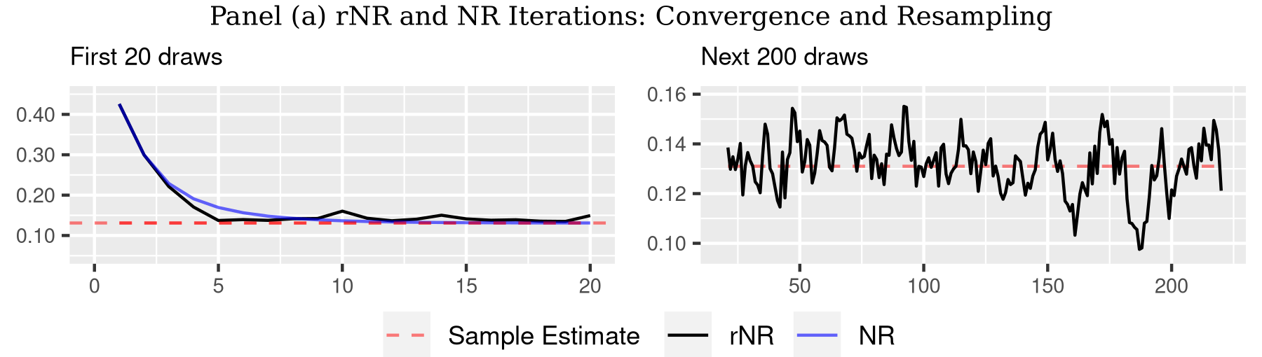
Figure 1: Labor force participation: draws for $\theta_{\text{educ}}$

Application 2: Earnings Dynamics

Moffitt and Zhang (2018) estimates earnings volatility using a subsample of $3508$ males in the Panel Study of Income Dynamics (PSID) dataset between 1970 and 2014 for a total of $36403$ observations. Let $y_{iat}$ denote an individual’s earnings $i$ in age group $a$ (between 24 and 54) at time $t$. Earnings are assumed to be the sum of a permanent $\mu_{ia}$ and a transitory $\nu_{iat}$ component:

$$y_{iat}=\alpha_{t}\mu_{ia}+\beta_{t}\nu_{ia},\quad\mu_{ia}=\mu_{i0}+\sum_{s=1}^{a}\omega_{is},\quad\nu_{ia}=\varepsilon_{ia}+\sum_{s=1}^{a}\psi_{a,a-s}\varepsilon_{is}\text{, for }a\geq 2.$$

In Moffitt and Zhang (2018), the variances are modeled via 11 parameters and estimated by a sequential quadratic programming algorithm (SQP). The Hessian in their example has both positive and negative eigenvalues, suggesting that the solution could be a saddle point. To abstract from identification issues, we estimate $\theta=(\nu_{0},\delta_{0},\gamma_{0},\gamma_{1})$ and fix the remaining 7 parameters. We specify the conditioning matrix as $P_{b}=(H_{b}^{\prime}H_{b})^{-1/2}$ to ensure positive definiteness. Algorithm 2 converges using the starting values $\theta_{0}=(0.054,-10.257,-4.355,0.012)$ as in the original paper, with $m=n$, $\gamma=0.2$ $B=2000$, and resampling at the age-cohort level. We also consider re-weighting instead of resampling which is denoted as rnr_w. Though our theory does not cover resampled quasi-Newton methods, we also use an implementation of bfgs that sets $P_{b}=(H_{b,\textsc{bfgs}}^{\prime}H_{b,\textsc{bfgs}})^{-1/2}$, where $H_{b,\textsc{bfgs}}$ is the bfgs approximation of the Hessian matrix, and report the results as rqn.

Table 5 shows that the rnr, rnr_w and rqn estimates are very close to $\hat{\theta}_{n}$ obtained by SQP. The rnr_w  standard errors are larger than the rnr  ones, which are in turn larger than the bootstrap ones, but the differences are not enough to change the conclusion that all four parameters are statistically different from zero. However, bootstrap inference of $\hat{\theta}_{n}$ is time-consuming, requiring 5h48m to produce 2000 draws, even after the original Matlab code was ported to r and C++ using Rcpp to get a greater than $10$ times speedup in computation time. In contrast, rnr  produces estimates and standard errors in 1h4m, and the rqn in 38m. The time needed for dmk  to produce standard errors is comparable to rnr, while rqn is more comparable to ks. However, both have an overhead of having to first obtain $\hat{\theta}_{n}$, which entails minimization of the objective function by SQP.

Table 5: Earnings Volatility: Estimates and Standard Errors

	Estimates					Standard Errors
	$\hat{\theta}_{n}$	rnr	rnrw	rqn	rqnw	boot	dmk	ks	rnr	rnrw	rqn	rqnw
$\nu_{0}$	0.109	0.109	0.109	0.109	0.109	0.002	0.002	0.002	0.002	0.002	0.002	0.002
$\delta_{0}$	-5.768	-5.779	-5.779	-5.767	-5.766	0.050	0.062	0.049	0.063	0.060	0.051	0.049
$\gamma_{0}$	-1.839	-1.819	-1.819	-1.841	-1.842	0.083	0.101	0.079	0.094	0.091	0.089	0.082
$\gamma_{1}$	0.010	0.011	0.011	0.010	0.010	0.010	0.012	0.010	0.011	0.012	0.011	0.011
					time	5h48m	1h4m	13m	1h4m	1h4m	38m	38m

In addition to providing standard errors, an additional by-product of Algorithm 2 is that the draws can be used for model diagnostics. Gentzkow et al. (2017) provides statistics to assess the sensitivity of the parameter estimates to assumptions of the model, taking the data as given. Our algorithm takes the model assumptions as given, but takes advantage of resampling to shed light on the sensitivity of the estimates to features of the data themselves. As pointed out in Chatterjee et al. (1986), influential observations could be outliers, or could be points of high leverage. If no such observations exist, removing them in the resampled data should not significantly affect the Markov chain. If their presence is influential, we should witness a ‘break’ in the draws.

With this motivation in mind, we examine whether the parameter estimates of the earnings model are sensitive to data of a particular age group.

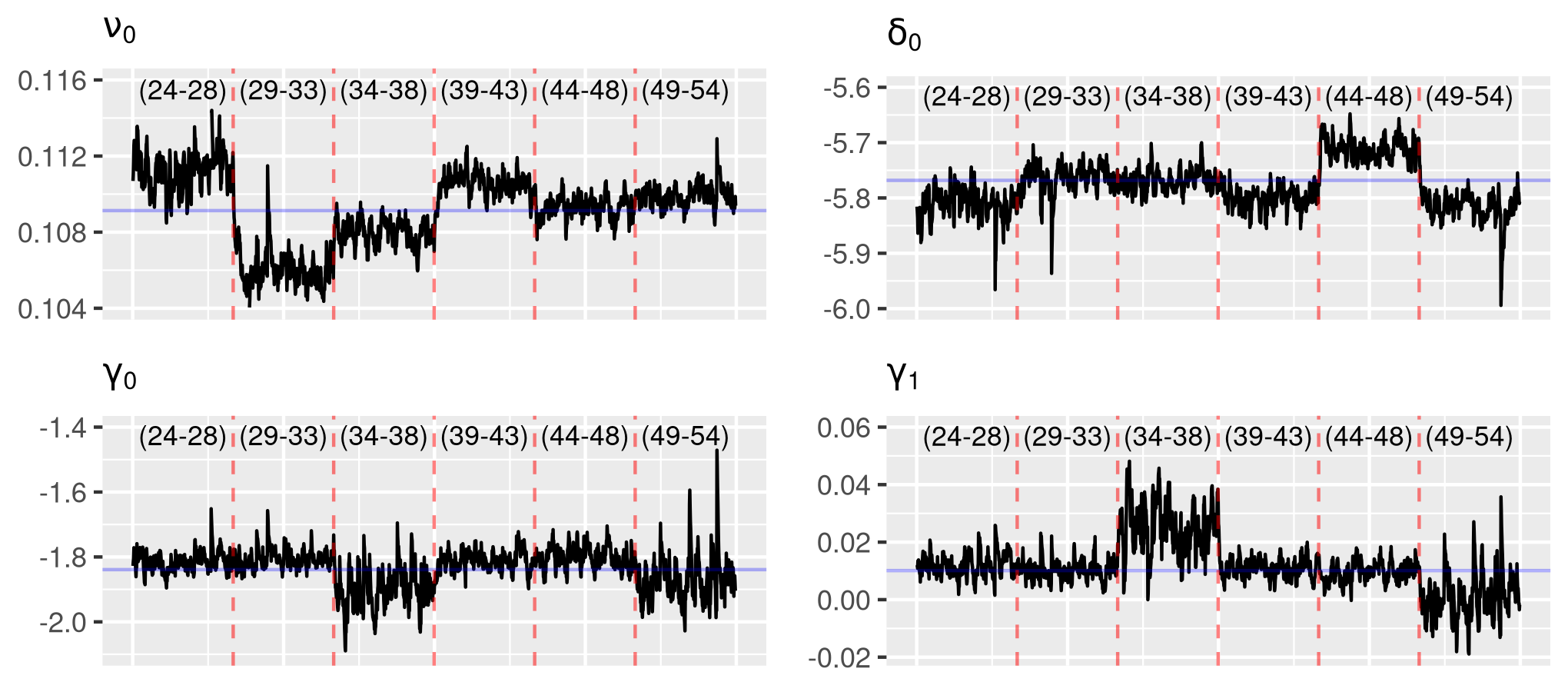
Figure 2: Earnings Volatility: Sensitivity to Age Groups

Legend: solid blue: full sample estimate; black line: rnr  draws excluding the age group indicated above in parenthesis; red dashed line: change in excluded age group

Figure 2 presents results for estimation based on resampled data that exclude one age group at a time. The parameter that is least sensitive to age-groups appears to be $\gamma_{1}$. The parameter $\nu_{0}$ tends to be lower when the age group (29-33) is excluded, while $\gamma_{0}$ is higher when the age group (44-48) is excluded. The parameter most sensitive to age is $\gamma_{0}$, which is evidently smaller in absolute magnitude when the younger age groups are excluded. For example, it is -1.2 when the youngest age group is dropped, but is around -2.0 when the oldest age group is excluded.

Application 3: Demand for Cereal

We evaluate the rnr  algorithm on the BLP model of Berry et al. (1995) using the cereal data generated in Nevo (2000). The sample consists of market shares for $24$ cereal products across $94$ markets for a total of $2256$ market/product observations. This example is of interest because bootstrapping the BLP model is demanding. We use the BLPestimatoR R package which builds on C++ functions to evaluate the GMM objective and analytical gradient. The data consists of market shares for 24 products in 94 markets. In the BLP framework, parameters on terms that enter linearly can projected out by 2SLS. Of the remaining parameters that need to be estimated, we drop some interaction terms from the original paper that may be difficult to identify. This allows us to focus on coefficients that enter the moment conditions non-linearly since the BLP procedure requires a fixed-point inversion for these, making the moment conditions costly to evaluate. The parameter dimension including market fixed effects is $d=33$. To control for possible correlations in the unobservables at the market level, we compute cluster-robust standard errors. See Appendix C for details

The data consists of market shares $s_{gj}$ in market $g\in\{1,\dots,94\}$ for product $j\in\{1,\dots,24\}$ with characteristic matrix $X_{gj}$. To resample at the market level, for each $b=1,\dots,B$ we draw markets $g^{(b)}_{1},\dots,g_{94}^{(b)}$ from $\{1,\dots,94\}$ with replacement and take the associated shares and characteristics $\{s_{g^{(b)}j},X_{g^{(b)}j}\}_{j=1,\dots,24}$ as observations within each market. Since the number of clusers is relatively small, we only consider $m=n$. We set $\gamma=0.2$ and a burn-in period of $10$ draws. Additional values of $\gamma$ are considered in Table C2. Both rnr  and rqn deliver estimates similar to those obtained from classical optimization and the standard errors are similar to the bootstrap ones. However, there is a significant difference. To generate $B=1000$ draws the standard bootstrap requires 4h45m while the rnr  runs in 1h04m which is almost 5x faster. The rqn estimate only requires 13m, which is about 20x faster than the bootstrap. While dmk  is similar to rnr, a preliminary estimate of $\theta$ is needed. Estimation of the AR(1) coefficient for the rnr  draws associated with the parameters reported in Table 6 finds that the estimates range from $0.78$ to $0.82$ with 95% confidence levels that always include the value of $(1-\gamma)=0.8$ predicted by theory.

For this example we also consider the CH quasi-Bayesian estimator implemented using a random walk Metropolis-Hastings MCMC algorithm. The prior for each of the $33$ parameters is a $\mathcal{N}(0,100)$ distribution, and the inverse of the clustered variance-covariance matrix of the moments evaluated at $\hat{\theta}_{n}$ is used as the optimal weighting matrix $W_{n}$. The Markov chain is initialized at $\theta_{0}=\hat{\theta}_{n}$, the proposal in the random walk step is scaled by $0.2H_{n}(\hat{\theta}_{n})^{-1/2}/\sqrt{n}$ which yields an acceptance rate of $0.335$. Though we generate a large number of draws ($B=50000$), the Markov chain is strongly persistent and the effective sample size as defined in Gelman et al. (2013) is typically less than $100$. The CH estimates are further away from $\hat{\theta}_{n}$ than the rnr  estimates, and the standard errors are also smaller than the $m$ out of $n$ bootstrap and the rnr  or the dmk.

Table 6: Demand for Cereal: Estimates and Standard Errors (Random Coefficients)

		Estimates				Standard Errors
		$\hat{\theta}_{n}$	ch	rnr	rqn	ch	boot	dmk	rnr	rqn
stdev	const.	0.284	-0.016	0.263	0.277	0.130	0.129	0.127	0.123	0.105
	price	2.032	2.364	2.188	1.917	0.738	1.198	1.026	0.975	0.880
	sugar	-0.008	-0.013	-0.006	-0.006	0.011	0.017	0.012	0.012	0.010
	mushy	-0.077	-0.248	-0.055	-0.042	0.132	0.177	0.168	0.166	0.154
income	const.	3.581	4.414	3.464	3.702	0.453	0.666	0.738	0.714	0.636
	price	0.467	-3.255	1.335	-0.295	2.449	3.829	4.275	4.040	3.603
	sugar	-0.172	-0.195	-0.171	-0.174	0.021	0.028	0.028	0.027	0.025
	mushy	0.690	0.888	0.647	0.702	0.203	0.345	0.346	0.339	0.312
					time	1h50m	4h45m	1h4m	1h8m	13m

6 Implications for Simulation-Based Estimation

Simulation-based estimation is routinely used to analyze structural models associated with analytically intractable likelihoods. Estimators in this class include the simulated method of moments, indirect inference and efficient method of moments, and following Forneron and Ng (2016), we will generically refer to them as simulated minimum distance (smd) estimators. We now show that rnr will still provide valid inference. This is useful because computing standard errors for the smd estimates is not always straightforward.

The minimum-distance (md) estimator minimizes the distance between a sample auxiliary statistic $\hat{\psi}_{n}=\hat{\psi}_{n}(\theta^{0})$ and it’s expected value $\psi(\theta)$ and is defined as

$$\hat{\theta}_{n,\textsc{md}}=\text{argmin}_{\theta}\|\overline{g}_{n}(\theta)\|^{2}_{W_{n}},\quad\overline{g}_{n}(\theta)=\hat{\psi}_{n}-\psi(\theta)\quad$$

where $W_{n}$ is a weighting matrix. In cases when the binding function $\psi(\cdot)$ that maps $\theta$ to the auxiliary statistic is tractable, Algorithm 2 provides a convenient way to compute standard errors for $\hat{\theta}_{n,\textsc{md}}$. When $\psi(\theta)$ is not tractable, smd simulates data $y_{i,s}(\theta)$ for given $\theta$ using iid errors $e_{i,s}$ and estimates $\psi(\theta)$ by $\hat{\psi}_{n,S}(\theta)=\frac{1}{S}\sum_{s=1}^{S}\psi_{n,s}(y_{n,s}(\theta))$. The estimator is

$$\hat{\theta}_{n,\textsc{smd}}=\text{argmin}_{\theta}\|\overline{g}_{n,S}(\theta)\|^{2}_{W_{n}}\quad\overline{g}_{n,S}(\theta)=\hat{\psi}_{n}-\hat{\psi}_{n,S}(\theta)\quad$$

To motivate our simulation based rnr, consider the exactly identified case when it holds that $\hat{\psi}_{n}-\psi(\hat{\theta}_{n,\textsc{md}})=0$. Note that while the vector of auxiliary statistics $\hat{\psi}_{m}^{(b)}$ computed using resampled data satisfies $\mathbb{E}^{\star}(\hat{\psi}_{m}^{(b)})=\hat{\psi}_{n}$, the statistics $\hat{\psi}_{m,S}^{(b)}(\theta)$ computed by smd  satisfies $\mathbb{E}^{\star}[\hat{\psi}_{m,S}^{(b)}(\theta)]=\psi(\theta)$, for all $\theta$. The two results together imply that $\mathbb{E}^{\star}[\hat{\psi}_{m}^{(b)}-\hat{\psi}_{m,S}^{(b)}(\theta)]$ when evaluated at $\theta=\hat{\theta}_{n,\textsc{md}}$ is $\hat{\psi}_{n}-\psi(\hat{\theta}_{n,\textsc{md}})$ which takes the value of zero as in md  estimation. This suggests a simulation based resampled objective function defined as:

$$Q_{m,S}^{(b)}(\theta)=\|\hat{\psi}_{m}^{(b)}-\hat{\psi}^{(b)}_{m,S}(\theta)\|^{2}_{W_{n}},\quad\overline{g}_{m,S}(\theta)=\hat{\psi}_{m}^{(b)}-\hat{\psi}_{m,S}^{(b)}(\theta)\quad$$

will have the same minimizer as the infeasible md, at least to a first-order. Let the draws be generated according $\theta_{b+1,S}=\theta_{b,S}-\gamma P_{b+1,S}G_{m,S}^{(b)}(\theta_{b})$ with gradient

$$G_{m,S}^{(b)}(\theta_{b,S})=-2\partial_{\theta^{\prime}}\hat{\psi}_{m,S}^{(b)}(\theta_{b,S})W_{n}(\hat{\psi}_{m}^{(b)}-\hat{\psi}_{m,S}^{(b)}(\theta)).$$ (12)

By Theorem 1, the mean $\overline{\theta}_{r\textsc{nr},S}$ is consistent for $\hat{\theta}_{n,\textsc{md}}$. By implication, $\theta_{\textsc{re},S}$ will also be more efficient than $\hat{\theta}_{n,\textsc{smd}}$, which we will verify in simulations below. To analyze $\overline{\theta}_{\textsc{re},S}$, we need the following:

Assumption 2.iii^′.

Suppose there exists finite constants $C_{7},C_{8}$ such that for any $S\geq 1$

• $\left[\mathbb{E}^{\star}\left(\|\hat{\psi}_{m}^{(b)}-\hat{\psi}_{n}\|_{2}^{4}\right)\right]^{1/4}\leq\frac{C_{7}}{\sqrt{m}}$; $\left[\mathbb{E}^{\star}\left(\sup_{\theta\in\Theta}\|\hat{\psi}_{m,S}^{(b)}(\theta)-\psi(\theta)\|_{2}^{4}\right)\right]^{1/4}\leq\frac{C_{7}}{\sqrt{mS}}$

• $\left[\mathbb{E}^{\star}\left(\|\partial_{\theta}\hat{\psi}_{m,S}^{(b)}(\hat{\theta}_{n})-\partial_{\theta}\psi(\hat{\theta}_{n})\|_{2}^{4}\right)\right]^{1/4}\leq\frac{C_{8}}{\sqrt{mS}}$.

Assumption 2.iii’ implies Assumption 2.iii where $G_{n}(\theta)$ is the gradient of md  by taking the difference $G_{m,S}^{(b)}(\theta)-G_{n}(\theta)$ and using the Cauchy-Schwarz inequality.

It remains to construct the variance of $\overline{\theta}_{r\textsc{nr},S}$. The foregoing analysis would suggest that valid inference would follow after the variance adjustment defined in Algorithm 2. However, this is not the case. Intuitively, the estimator $\overline{\theta}_{r\textsc{nr},S}$ is consistent for $\hat{\theta}_{n,\textsc{md}}$ whose variance $\mathbb{V}^{0}$ does not involve simulation noise. But the quantity $V_{r\textsc{nr}}$ defined in Algorithm 2 presumes the presence of simulation noise in the estimate $\overline{\theta}_{r\textsc{nr},S}$ and will give standard errors that will, in general, be too large. The are many ways to overcome this problem, and most involve running a second chain of draws in parallel with the one used to compute the estimator. For example, taking the difference of two chains with the same simulated samples would work as the simulation noise will offset.

Our preferred approach is to use a second chain that directly estimates the variance of $\overline{\theta}_{r\textsc{nr},S}$. As in the first chain, this second chain is generated as $\theta^{2}_{b+1,S}=(1-\gamma)\theta^{2}_{b,S}-\gamma P_{b+1,S}\tilde{G}_{m,S}^{(b)}(\theta_{b,S}^{2})$ as defined in (7), but the gradient is

$$\tilde{G}^{(b)}_{m,S}(\theta^{1}_{b,S})=-2\partial_{\theta^{\prime}}\hat{\psi}_{m,S}^{(b)}(\theta^{1}_{b,S})W_{n}(\hat{\psi}_{m}^{(b)}-\hat{\psi}_{n}).$$ (13)

Compared to the first chain defined by (12), the second chain replaces the simulated auxiliary statistics $\hat{\psi}_{m,S}^{(b)}(\hat{\theta}_{n})$ by the sample estimates $\hat{\psi}_{n}$ which is already computed. As all other quantities involved in computing (13) are taken from (12), the computation overhead of generating $\theta^{2}_{b,S}$ is thus negligible.

Proposition 1.

Suppose that the Assumptions for $Q_{n}$ and $Q^{(b)}_{m,S}$ in Theorems 1 and 2 hold, with Assumption 2.iii replaced by 2.iii’. Let $\hat{\theta}_{n,\textsc{md}}$ be the infeasible minimum-distance estimator. Let $\{\theta^{1}_{b,S}\}$ be a chain generated with $G^{(b)}_{m,S}$ defined as in (12), and $\{\theta^{2}_{b,S}\}$ be generated using $\tilde{G}_{m,S}^{(b)}$ defined as in (13). Let $\overline{\theta}_{r\textsc{nr},S}=\frac{1}{B}\sum_{b=1}^{B}\theta_{b,S}^{1}$, $P_{b+1,S}=[H_{m,S}^{(b+1)}(\theta^{1}_{b,S})]^{-1}$, and define $\mathbb{V}_{r\textsc{nr},S}=\frac{m}{\phi(\gamma)}\text{var}^{\star}(\theta_{b,S}^{2})$. Then for any $S\geq 1$ fixed,

• $\sqrt{n}\left(\overline{\theta}_{r\textsc{nr},S}-\theta^{0}\right)=\sqrt{n}\left(\hat{\theta}_{n,\textsc{md}}-\theta^{0}\right)+o_{p^{\star}}(1)$.

• As $m,b\to+\infty$ with $\log(m)/b\to 0$:

  $$\mathbb{V}_{r\textsc{nr},S}^{-1/2}\sqrt{n}\left(\overline{\theta}_{r\textsc{nr},S}-\theta^{0}\right)\overset{d^{\star}}{\to}\mathcal{N}\left(0,I_{d}\right),$$

Forneron and Ng (2016, 2018) shows that a weighted average of smd estimates with independent simulation draws constitutes a posterior mean which is asymptotically equivalent to the infeasible md estimator. This requires solving the optimization problem as many times (ie. $S>1$). Part i. of the proposition shows that this type of statistical efficiency can be achieved by rnr  in a single run, ie($S=1$). Resampling by rnr  involves taking draws from the joint distribution $F_{n}\times F_{\text{shocks}}$ to produce $\hat{\psi}^{(b)}_{m,S}(\theta)$, which is an estimate of population mapping $\psi(\theta)$. In practice, the simulation and resampling noise in $\hat{\psi}^{(b)}_{m,S}(\theta)$ and $\hat{\psi}_{m}^{(b)}$ are averaged out so that the variance of $\overline{\theta}_{r\textsc{nr},S}$ does not depend on $S$ asymptotically. This contrasts with the smd estimator $\hat{\theta}_{n,\textsc{smd}}$ which has vanishing simulation noise only when $S\rightarrow\infty$ as $n\to\infty$.

Part ii of the Proposition involves a second sequence $\theta^{2}_{b,S}$ which, as noted above, is used to compute the variance of the estimator. To understand its underpinnings, recall that the sandwich variance for $\hat{\theta}_{n,\textsc{md}}$ has a meat component that is the variance of the score $-2\partial_{\theta^{\prime}}\psi(\hat{\theta}_{n,\textsc{md}})W_{n}(\hat{\psi}_{n}-\psi(\hat{\theta}_{n,\textsc{md}}))$. If $\psi$ were tractable, a bootstrap draw of this score would be $-2\partial_{\theta^{\prime}}\psi(\hat{\theta}_{n,\textsc{md}})W_{n}(\hat{\psi}_{m}^{(b)}-\psi(\hat{\theta}_{n,\textsc{md}}))$. But this is approximately $-2\partial_{\theta^{\prime}}\hat{\psi}_{m,S}^{(b)}(\theta_{b,S}^{1})W_{n}(\hat{\psi}_{m}^{(b)}-\hat{\psi}_{n})$ which is precisely the gradient (13) used to generate $\theta_{b,S}^{2}$. Hence it provides a correct approximation of the variance of the scores. Though two chains are needed in the case of simulation estimation, it only needs $S=1$. These arguments are further illustrated using a simple example in Appendix D.

Example 3: Dynamic Panel

Consider the dynamic panel regression:

$$y_{it}=\alpha_{i}+\rho y_{it-1}+x_{it}^{\prime}\beta+\sigma_{e}e_{it},$$

with $\rho=0.6,\beta=1,\sigma_{e}=1$, $x_{it}\sim\mathcal{N}(0,1),e\sim\mathcal{N}(0,1)$, $n=1000$ and $T=5$. Let $A=I_{T}-1_{T}1_{T}^{\prime}/T$, a matrix which computes the time de-meaned $y_{it}-\overline{y}_{i}$. The Least-Squares Dummy Variable (LSDV) estimator is obtained by regressing $Ay_{2:T}$ on $Ay_{1:T-1}$ and $Ax_{2:T}$. The estimator is inconsistent for fixed $T$ as $n\to\infty$.

The LSDV estimator is inconsistent when $n\to\infty$ and $T$ is fixed. Gouriéroux et al. (2010) shows that indirect inference, which has an automatic bias correction property, is consistent for fixed $T$. The idea is to match the sample LSDV estimator $\hat{\psi}_{n}=\hat{\theta}_{n,LSDV}$ with a simulated $\hat{\psi}_{n,S}(\theta)=\hat{\theta}^{sim}_{n,LSDV}(\theta)$ using $S\geq 1$ simulated samples.

To generate rnr  draws, we resample $(y_{i1},\dots,y_{iT},x_{i1},\dots,x_{iT})_{i=1,\dots,m}$ with replacement over $i$ for given $m$ and compute $\hat{\psi}_{m}^{(b)}=\hat{\theta}_{m,LSDV}^{(b)}$, our resampled moments. Using the new simulation draws $e^{(b+1)}_{it}$ at each $b$, we simulate $S\geq 1$ panels: $y^{(b+1)}_{it,s}=\rho y_{it-1,s}+x_{it,s}^{(b+1)\prime}\beta+\sigma_{e}e^{(b+1)}_{it,s}$, for $t=1,\dots,T$ and $i=1,\dots,m$ and compute the simulated moments $\hat{\psi}_{m,S}^{(b)}=\tilde{\theta}_{m,LSDV}^{(b)}(\theta_{b})$. An addional moment is needed to estimate $\sigma_{e}$; we use the standard deviation of the OLS residuals in the LSVD regression. The gradient and Hessian are computed using finite differences. We illustrate with $m=n,100,50$ for $n=1000$.

Table 7: Dynamic Panel: Estimates of $\rho$ and Standard Errors

		Estimates				Standard Errors
$S$	$m$	ind	rnr0.3	rnr0.1	rnr0.01	ase	boot	dmk	rnr0.3	rnr0.1	rnr0.01
	$200$	0.619	0.589	0.592	0.590	0.045	0.049	0.050	0.034	0.034	0.025
1	$100$	-	0.589	0.588	0.586	-	0.048	-	0.036	0.039	0.037
	$50$	-	0.580	0.588	0.581	-	0.050	-	0.037	0.037	0.024
	$200$	0.584	0.591	0.589	0.589	0.035	0.036	0.036	0.035	0.036	0.032
10	$100$	-	0.589	0.591	0.587	-	0.034	-	0.034	0.037	0.030
	$50$	-	0.586	0.589	0.587	-	0.035	-	0.038	0.031	0.032

Remark: Results reported for one simulated sample of size $n=200,T=5$.

The LSDV estimate is 0.329 which is significantly downward biased. However, the indirect inference (ind) estimator corrects the bias as shown in Gouriéroux et al. (2010). The estimate of $0.619$ in Table 7 for $S=1$ bears this out. The rnr  estimates are closer to $\theta^{0}$ than ind for $m=n$, $100$ and is similar for $m=50$. The ind estimates with $S=10$ are very close to the rnr  estimates obtained over all $\gamma,m$ and $S$ including $S=1$. This implies that rnr  achieves the efficiency of ind with large $S$ using just $S=1$. The standard errors are smaller than other methods except for $S=10$. Results for $S=2,5$ are reported in Table D1.

We close the analysis with two remarks about the examples. As noted earlier, an ill-conditioned Hessian can render slow convergence of gradient-based optimizers. The values of $\frac{\lambda_{\text{min}}(H_{n})}{\lambda_{\text{max}}(H_{n})}$ evaluated at $\theta=\hat{\theta}_{n}$, are $10^{-7},8\cdot 10^{-4}$ and $7\cdot 10^{-6}$ for the probit, earnings dynamics, and BLP examples, respectively. Classical gd should be slow in converging in these cases, and the applications bear this out. Second, to reinforce the main result that Algorithm 2 provides valid inference, we evaluate the coverage of rnr  in all of the simulated examples considered. As seen from Table 8, rnr  delivers a 5% size in almost all cases. Details are given in Appendix C of the online supplement.

Table 8: Size of Confidence Intervals Across Methods and Examples

		ase	boot	dmk	ks	rnr	boot	rnr
OLS			$m=n=200$				$m=50$
	$\beta_{0}$	0.044	0.043	0.043	0.041	0.049	0.040	0.047
	$\beta_{1}$	0.045	0.056	0.056	0.070	0.069	0.043	0.048
MA(1)			$m=n=500$				$m=250$
	$\mu$	0.291	0.048	0.294	-	0.183	0.051	0.169
	$\psi$	0.066	0.047	0.067	-	0.064	0.035	0.044
			$m=n=1000$				$m=100$
Dynamic	$\rho$	0.055	0.047	0.044	-	0.050	0.052	0.040
Panel	$\beta$	0.055	0.054	0.051	-	0.057	0.051	0.049
($S=1$)	$\sigma$	0.060	0.053	0.046	-	0.057	0.052	0.059
			$m=n=1000$				$m=100$
Dynamic	$\rho$	0.051	0.054	0.055	-	0.053	0.059	0.053
Panel	$\beta$	0.040	0.046	0.046	-	0.049	0.045	0.049
($S=2$)	$\sigma$	0.065	0.056	0.053	-	0.056	0.056	0.056
			$m=n=1000$				$m=100$
Dynamic	$\rho$	0.052	0.054	0.053	-	0.048	0.051	0.050
Panel	$\beta$	0.040	0.047	0.042	-	0.036	0.043	0.038
($S=5$)	$\sigma$	0.065	0.058	0.056	-	0.064	0.061	0.061

Results based on $1000$ replications with $B=1000,\gamma=0.1$; burn=45.

7 Conclusion

In this paper, we design two algorithms to produce draws that, upon averaging, is asymptotically equivalent to the full-sample estimate produced by a classical optimizer. By using the inverse Hessian as conditioning matrix, the draws of Algorithm 2 immediately provide valid standard errors for inference, hence a free lunch. In problems that require $S$ simulations to approximate the binding function, our algorithm achieves the level of efficiency of smd with a large $S$, but at the cost of $S=1$. Numerical evaluations show that Algorithm 2 produces accurate estimates and standard errors but runs significantly faster than the conventional bootstrap and most of the ‘short-cut’ methods.

Appendix A

A.1 Derivations for the Least-Squares Example

In this example, $y_{n}=X_{n}\hat{\theta}_{n}+\hat{e}_{n}$, $Q_{n}(\theta)=\frac{1}{2n}(y_{n}-X_{n}\theta)^{\prime}(y_{n}-X_{n}\theta)$, $H_{n}=X_{n}^{\prime}X_{n}/n,G_{n}=-X_{n}^{\prime}\hat{e}_{n}/n$, and $Q_{m}^{(b)}(\theta)=\frac{1}{2m}(y_{m}^{(b)}-X_{m}^{(b)}\theta)^{\prime}(y_{m}^{(b)}-X_{m}^{(b)}\theta)$, $H_{b}=H^{(b+1)}_{m}(\theta_{b})=X^{(b+1)^{\prime}}_{m}X^{(b+1)}_{m}/m$. $G_{b}(\theta)=-X_{m}^{(b+1)^{\prime}}[y_{m}^{(b+1)}-X_{m}^{(b+1)}\theta]/m$. Let $\hat{\theta}_{m}^{(b+1)}=(X_{m}^{(b+1)\prime}X_{m}^{(b+1)})^{-1}X_{m}^{(b+1)\prime}y_{m}^{(b+1)}$ be the $m$ out of $n$ bootstrap estimate. Orthogonality of least squares residuals will be used repeatedly.

Gradient Descent

$\theta_{k+1}=\theta_{k}-\gamma\left[-X_{n}^{\prime}(y_{n}-X_{n}\theta_{k})/n\right]$. Subtract $\hat{\theta}_{n}$ on both sides and note that $y_{n}=X_{n}\hat{\theta}_{n}+\hat{e}_{n}$ (full sample estimates), then:

$$\theta_{k+1}-\hat{\theta}_{n} =\theta_{k}-\hat{\theta}_{n}-\gamma\left[-X_{n}^{\prime}(X_{n}\hat{\theta}_{n}+\hat{e}_{n}-X_{n}\theta_{k})/n\right]$$

$$=\theta_{k}-\hat{\theta}_{n}-(\gamma H_{n})(\theta_{k}-\hat{\theta}_{n})+\gamma X_{n}^{\prime}\hat{e}_{n}/n=(I-\gamma H_{n})(\theta_{b}-\hat{\theta}_{n})\quad\text{since }X_{n}^{\prime}\hat{e}_{n}=0.$$

Newton-Raphson

$\theta_{k+1}=\theta_{k}-\gamma\left[H_{n}\right]^{-1}\left[-X_{n}^{\prime}(y_{n}-X_{n}\theta_{k})/n\right].$ Subtract $\hat{\theta}_{n}$ on both sides:

$$\theta_{k+1}-\hat{\theta}_{n} =\theta_{k}-\hat{\theta}_{n}-\gamma H_{n}^{-1}\left[-[X_{n}^{\prime}X_{n}/n][\hat{\theta}_{n}-\theta_{k}]+X_{n}^{\prime}\hat{e}_{n}/n\right]=(1-\gamma)(\theta_{k}-\hat{\theta}_{n})\quad\text{since }X_{n}^{\prime}\hat{e}_{n}=0.$$

Stochastic Gradient Descent

$\theta_{b+1}=\theta_{b}-\gamma_{b}\left[-X_{m}^{(b)\prime}(y_{m}^{(b)}-X_{m}^{(b)}\theta_{b})/m\right]$. Thus

$$\theta_{b+1}-\hat{\theta}_{n} =\theta_{b}-\hat{\theta}_{n}-\gamma_{b}\left[-X_{m}^{(b+1)\prime}(y_{m}^{(b+1)}-X_{m}^{(b+1)}\hat{\theta}_{n}-X_{m}^{(b+1)}[\theta_{b}-\hat{\theta}_{n}])/m\right]$$

$$=(I-\gamma_{b}H_{b})(\theta_{b}-\hat{\theta}_{n})+\gamma_{b}X_{m}^{(b+1)\prime}(y_{m}^{(b+1)}-X_{m}^{(b+1)}\hat{\theta}_{n})/m$$

$$=(I-\gamma_{b}H_{b})(\theta_{b}-\hat{\theta}_{n})-\gamma_{b}G_{b}(\hat{\theta}_{n})\quad\text{since }X_{m}^{(b+1)^{\prime}}\hat{e}_{m}^{(b+1)}=0.$$

Resampled Gradient Descent

$\theta_{b+1}=\theta_{b}-\gamma\left[-X_{m}^{(b+1)\prime}(y_{m}^{(b+1)}-X_{m}^{(b+1)}\theta_{b})/m\right]$. Subtract $\hat{\theta}_{n}$ on both sides and note that $y_{m}^{(b+1)}=X_{m}^{(b+1)}\hat{\theta}_{m}^{(b+1)}+\hat{e}_{m}^{(b+1)}$ (bootstrap estimates). Then

$$\theta_{b+1}-\hat{\theta}_{n} =\theta_{b}-\hat{\theta}_{n}-\gamma\left[-X_{m}^{(b+1)\prime}(X_{m}^{(b+1)}[\hat{\theta}_{m}^{(b+1)}-\hat{\theta}_{n}]+\hat{e}_{m}^{(b+1)}-X_{m}^{(b+1)}[\theta_{b}-\hat{\theta}_{n}])/m\right]$$

$$=\theta_{b}-\hat{\theta}_{n}-(\gamma H_{b})(\theta_{b}-\hat{\theta}_{n})+\gamma H_{b}(\hat{\theta}_{m}^{(b)}-\hat{\theta}_{n})$$

$$=(I-\gamma H_{b})(\theta_{b}-\hat{\theta}_{n})+\gamma H_{b}(\hat{\theta}_{m}^{(b+1)}-\hat{\theta}_{n})\quad\text{since }X_{m}^{(b+1)^{\prime}}\hat{e}_{m}^{(b+1)}=0.$$

Resampled Newton-Raphson

$\theta_{b+1}=\theta_{b}-\gamma[H_{b}]^{-1}\left[-X_{m}^{(b+1)\prime}(y_{m}^{(b+1)}-X_{m}^{(b+1)}\theta_{b})/m\right]$. Then

$$\theta_{b+1}-\hat{\theta}_{n} =\theta_{b}-\hat{\theta}_{n}-\gamma[H_{b}]^{-1}\left[-X_{m}^{(b+1)\prime}(X_{m}^{(b+1)}[\hat{\theta}_{m}^{(b+1)}-\hat{\theta}_{n}]+\hat{e}_{m}^{(b+1)}-X_{m}^{(b+1)}[\theta_{b}-\hat{\theta}_{n}])/m\right]$$

$$=(1-\gamma)(\theta_{b}-\hat{\theta}_{n})+\gamma(\hat{\theta}_{m}^{(b+1)}-\hat{\theta}_{n})\quad\text{since }X_{m}^{(b+1)\prime}\hat{e}_{m}^{(b+1)}=0.$$

A.2 Proof of Lemma 3:

Note first that by construction,

$$\gamma \left(P_{b}G_{m}^{(b+1)}(\theta_{b})-\overline{P}_{m}G_{m}^{(b+1)}(\hat{\theta}_{n})\right)=\gamma\overline{P}_{m}H_{n}(\hat{\theta}_{n})[\theta_{b}-\hat{\theta}_{n}]$$

$$\quad+\gamma\overline{P}_{m}\left(G_{m}^{(b+1)}(\theta_{b})-G_{m}^{(b+1)}(\hat{\theta}_{n})-H_{n}(\hat{\theta}_{n})[\theta_{b}-\hat{\theta}_{n}]\right)$$ (A.1)

$$\quad+\gamma\left(P_{b}-\overline{P}_{m}\right)\left(G_{m}^{(b+1)}(\theta_{b})-G_{m}^{(b+1)}(\hat{\theta}_{n})\right).$$ (A.2)

From the definition of $\theta_{b}$ and $\theta_{b}^{\star}$, the difference can be expressed as:

$$\theta_{b+1}-\theta_{b+1}^{\star} =\left(\theta_{b}-\gamma P_{b}G_{m}^{(b+1)}(\theta_{b})\right)-\left(\hat{\theta}_{n}+\Psi(\hat{\theta}_{n})(\theta_{b}^{\star}-\hat{\theta}_{n})-\gamma\overline{P}_{m}G_{m}^{(b+1)}(\hat{\theta}_{n})\right)$$

$$=\Psi(\hat{\theta}_{n})(\theta_{b}-\theta_{b}^{\star})+(I_{d}-\Psi(\hat{\theta}_{n}))(\theta_{b}-\hat{\theta}_{n})-\gamma\left(P_{b}G_{m}^{(b+1)}(\theta_{b})-\overline{P}_{m}G_{m}^{(b+1)}(\hat{\theta}_{n})\right)$$

$$=\Psi(\hat{\theta}_{n})(\theta_{b}-\theta_{b}^{\star})+\gamma\overline{P}_{m}H_{n}(\hat{\theta}_{n})[\theta_{b}-\hat{\theta}_{n}]-\gamma\left(P_{b}G_{m}^{(b+1)}(\theta_{b})-\overline{P}_{m}G_{m}^{(b+1)}(\hat{\theta}_{n})\right)$$

$$=\Psi(\hat{\theta}_{n})(\theta_{b}-\theta_{b}^{\star})-(\ref{eq:d3})-(\ref{eq:d4})$$

where the third equality follows from the fact that $I_{d}-\Psi(\hat{\theta}_{n})=\gamma\overline{P}_{m}H_{n}(\hat{\theta}_{n})$. By Assumption 2 i. and vi. as well as Lemma 2,

$$\mathbb{E}^{\star}(\|(\ref{eq:d3})\|_{2}) \leq\gamma\overline{\lambda}_{P}C_{2}\mathbb{E}^{\star}(\|\theta_{b}-\hat{\theta}_{n}\|_{2}^{2})$$

$$\leq 3\gamma\overline{\lambda}_{P}C_{2}\left((1-\overline{\gamma})^{2b+2}d_{0,n}^{2}+\frac{C_{5}^{2}}{\overline{\gamma}^{2}m}\right).$$

By Assumptions 2 ii., 3 ii., Lemma 2, mean-value theorem, and Cauchy-Schwarz inequality,

$$\mathbb{E}^{\star}\left(\|(\ref{eq:d4})\|_{2}\right) \leq\gamma\left[\mathbb{E}^{\star}\left(\|P_{b}-\overline{P_{m}}\|_{2}^{2}\right)\right]^{1/2}\left[\mathbb{E}^{\star}\left(\|H_{m}^{(b+1)}(\tilde{\theta}_{b})(\theta_{b}-\hat{\theta}_{n})\|_{2}^{2}\right)\right]^{1/2}$$

$$\leq\gamma\overline{\lambda}_{H}C_{6}\left(\overline{\rho}^{b}d_{0,n}+\frac{1}{\sqrt{m}}\right)\left((1-\overline{\gamma})^{b+1}d_{0,n}+\frac{C_{5}}{\overline{\gamma}\sqrt{m}}\right),$$

where $\tilde{\theta}_{b}$ is some intermediate value between $\theta_{b}$ and $\hat{\theta}_{n}$, and an upper bound defined in terms of $\overline{\rho}$ to simplify notation.

The two bounds leads to the following recursion on the coupling distance:

$$\mathbb{E}^{\star}\left(\|\theta_{b+1}-\theta_{b+1}^{\star}\|_{2}\right) \leq\overline{\rho}\mathbb{E}^{\star}\left(\|\theta_{b}-\theta_{b}^{\star}\|_{2}\right)+\mathbb{E}^{\star}(\|(\ref{eq:d3})\|_{2})+\mathbb{E}^{\star}(\|(\ref{eq:d4})\|_{2})$$

$$\leq\overline{\rho}\mathbb{E}^{\star}\left(\|\theta_{b}-\theta_{b}^{\star}\|_{2}\right)+C_{6}^{+}(\overline{\rho}^{b}[d_{0,n}+d_{0,n}^{2}]+\frac{1}{m})$$

$$\leq\frac{C_{6}^{+}}{1-\overline{\rho}}\left(\overline{\rho}^{b}[d_{0,n}+d_{0,n}^{2}]+\frac{1}{m}\right),$$

where $C_{6}^{+}$ is a constant which depends on the terms used to bound (A.1) and (A.2). Recall that $\theta_{0}=\theta_{0}^{\star}$ so that the coupling distance is zero for $b=0$. Putting $C_{7}=C_{6}^{+}/(1-\overline{\rho})$ proves the desired result.∎

A.3 Proof of Theorem 1

To bound $\mathbb{E}^{\star}\left(\|\overline{\theta}_{\textsc{re}}^{\star}-\hat{\theta}_{n}\|_{2}\right)$, we use the recursive representation of (7) and take the average:

$$\overline{\theta}_{\textsc{re}}^{\star}-\hat{\theta}_{n} =\frac{1}{B}\sum_{b=1}^{B}\Psi(\hat{\theta}_{n})^{b}(\theta_{0}-\hat{\theta}_{n})-\gamma\frac{1}{B}\sum_{b=1}^{B}\sum_{j=0}^{b-1}\Psi(\hat{\theta}_{n})^{j}\overline{P}_{m}\mathbb{E}^{\star}\left(G_{m}^{(b-j)}(\hat{\theta}_{n})\right)$$

$$-\gamma\frac{1}{B}\sum_{b=1}^{B}\sum_{j=0}^{b-1}\Psi(\hat{\theta}_{n})^{j}\overline{P}_{m}\underbrace{\left[G_{m}^{(b-j)}(\hat{\theta}_{n})-\mathbb{E}^{\star}\left(G_{m}^{(b-j)}(\hat{\theta}_{n})\right)\right]}_{\Delta_{m}^{(b-j)}(\hat{\theta}_{n})}.$$

Assumption 3 i. implies that $\|\Psi(\hat{\theta}_{n})^{b}(\theta_{0}-\hat{\theta}_{n})\|_{2}\leq\overline{\rho}^{b}\|\theta_{0}-\hat{\theta}_{n}\|_{2}$, so the first term is less than $\frac{d_{0,n}}{(1-\overline{\rho})B}$ in expectation. Consider now the second term. By Assumption 2 iv, $\|\Psi(\hat{\theta}_{n})^{j}\overline{P}_{m}\mathbb{E}^{\star}\left(G_{m}^{(b-j)}(\hat{\theta}_{n})\right)\|_{2}\leq\overline{\rho}^{j}\overline{\lambda}_{P}\frac{C_{3}^{\prime}}{\sqrt{m}}$ so the second term is less than $\frac{\overline{\lambda}_{P}C_{3}^{\prime}}{(1-\overline{\rho})\sqrt{m}}$. For the third term and with $\Delta_{m}^{(b-j)}(\hat{\theta}_{n})$ defined above, we have by conditional independence,

$$\bigg{[}\mathbb{E}^{\star}\left(\|\frac{1}{B}\sum_{b=1}^{B}\sum_{j=0}^{b-1}\Psi(\hat{\theta}_{n})^{j}\overline{P}_{m}\Delta_{m}^{(b-j)}(\hat{\theta}_{n})\|_{2}^{2}\right)\bigg{]}^{1/2} =\bigg{[}\mathbb{E}^{\star}\left(\|\frac{1}{B}\sum_{b=1}^{B}\sum_{j=0}^{B-b+1}\Psi(\hat{\theta}_{n})^{j}\overline{P}_{m}\Delta_{m}^{(b)}(\hat{\theta}_{n})\|_{2}^{2}\right)\bigg{]}^{1/2}$$

$$=\frac{1}{\sqrt{mB}}\bigg{[}\frac{1}{B}\sum_{b=1}^{B}\mathbb{E}^{\star}\left(\|\sum_{j=0}^{B-b+1}\Psi(\hat{\theta}_{n})^{j}\sqrt{m}\overline{P}_{m}\Delta_{m}^{(b)}(\hat{\theta}_{n})\|_{2}^{2}\right)\bigg{]}^{1/2}$$

$$\leq\frac{\overline{\lambda}_{P}}{(1-\overline{\rho})\sqrt{mB}}\bigg{[}\left(\sup_{1\leq b\leq B}\mathbb{E}^{\star}\|\sqrt{m}\Delta_{m}^{(b)}(\hat{\theta}_{n})\|_{2}^{2}\right)\bigg{]}^{1/2}$$

$$\leq\frac{\gamma\overline{\lambda}_{P}[C_{3}+C_{3}^{\prime}]}{(1-\overline{\rho})\sqrt{mB}}$$

where the first inequality follows from the average being less than the $\sup$, combined with $\|\Psi(\hat{\theta}_{n})^{j}\overline{P}_{m}\Delta_{m}^{(b)}(\hat{\theta}_{n})\|\leq\overline{\rho}^{j}\overline{\lambda}_{P}\|\Delta_{m}^{(b)}(\hat{\theta}_{n})\|$ which is summable over $j\geq 0$. The last inequality uses Assumption 2 iii-iv. Recall that Lemma 3 implies (9) which states that $\mathbb{E}^{\star}\bigg{(}\|\overline{\theta}_{\textsc{re}}-\overline{\theta}^{\star}_{\textsc{re}}\|_{2}\bigg{)}\leq\frac{C_{7}}{1-\overline{\rho}}\bigg{(}\frac{1}{m}+\frac{d_{0,n}+d_{0,n}^{2}}{B}\bigg{)}$. Now putting everything together, we have:

$$\mathbb{E}^{\star}\left(\|\overline{\theta}_{\textsc{re}}-\hat{\theta}_{n}\|_{2}\right) \leq\mathbb{E}^{*}\bigg{(}\|\overline{\theta}_{\textsc{re}}-\overline{\theta}_{\textsc{re}}^{*}\|_{2}\bigg{)}+\mathbb{E}^{*}\bigg{(}\overline{\theta}_{\textsc{re}}^{*}-\hat{\theta}_{n}\|_{2}\bigg{)}$$

$$\leq C_{8}\left(\frac{1}{m}+\frac{d_{0,n}+d_{0,n}^{2}}{B}+\frac{1}{\sqrt{mB}}\right),$$

which is a $o(\frac{1}{\sqrt{n}})$ when $\frac{\sqrt{n}}{\text{min}(m,B)}\to 0$ and $d_{0,n}=O(1)$.∎

A.4 Proof of Theorem 2

The property that $\overline{P}_{m}=[H_{n}(\hat{\theta}_{n})]^{-1}$ when $P_{b}=[H_{m}^{(b+1)}(\theta_{b})]^{-1}$ is crucial for what is to follow, and it is useful to understand why. Under Assumption 2 vi.,

$$\left[\mathbb{E}^{\star}\left(\|I_{d}-P_{b}H_{n}(\hat{\theta}_{n})\|_{2}^{2}\right)\right]^{1/2}\leq\frac{1}{\underline{\lambda}_{P}}\left[\mathbb{E}^{\star}\left(\|P_{b}^{-1}-H_{n}(\hat{\theta}_{n})\|_{2}^{2}\right)\right]^{1/2}.$$

Given that $P_{b}=[H_{m}^{(b+1)}(\theta_{b})]^{-1}$, an application of the triangular inequality, Assumption 1 ii. and 2 v. together with Lemma 2 give

$$\left[\mathbb{E}^{\star}\left(\|P_{b}^{-1}-H_{n}(\hat{\theta}_{n})\|_{2}^{2}\right)\right]^{1/2} =\left[\mathbb{E}^{\star}\left(\|H_{m}^{(b)}(\theta_{b})-H_{n}(\hat{\theta}_{n})\|_{2}^{2}\right)\right]^{1/2}$$

$$\leq\left[\mathbb{E}^{\star}\left(\|H_{n}(\theta_{b})-H_{n}(\hat{\theta}_{n})\|_{2}^{2}\right)\right]^{1/2}+\left[\mathbb{E}^{\star}\left(\|H_{m}^{(b+1)}(\theta_{b})-H_{n}(\theta_{b})\|_{2}^{2}\right)\right]^{1/2}$$

$$\leq C_{1}\left[\mathbb{E}^{\star}\left(\|\theta_{b}-\hat{\theta}_{n}\|_{2}^{2}\right)\right]^{1/2}+\left[\mathbb{E}^{\star}\left(\sup_{\theta\in\Theta}\|H_{m}^{(b+1)}(\theta)-H_{n}(\theta)\|_{2}^{2}\right)\right]^{1/2}$$

$$\leq(1-\overline{\gamma})^{b}C_{1}d_{0,n}+\left(\frac{C_{1}C_{5}}{\overline{\gamma}}+C_{4}\right)\frac{1}{\sqrt{m}}.$$

This implies that Assumption 3 ii. holds with $C_{6}=\text{max}(C_{1},\frac{C_{1}C_{5}}{\overline{\gamma}}+C_{4})$ and $\overline{P}_{m}=[H_{n}(\hat{\theta}_{n})]^{-1}$. Assumption 3 i. automatically holds since we now have $\Psi(\hat{\theta}_{n})=(1-\gamma)I_{d}$ which has all its eigenvalues in $[0,1)$ for any $\gamma\in(0,1]$.

To prove Theorem 2, we first substitute $\theta_{b}$ for the linear process $\theta_{b}^{\star}$ using:

$$\frac{\sqrt{m}}{\sqrt{\phi(\gamma)}}(\mathbb{V}^{m})^{-1/2}(\theta_{b}-\hat{\theta}_{n})=\frac{\sqrt{m}}{\sqrt{\phi(\gamma)}}(\mathbb{V}^{m})^{-1/2}(\theta_{b}-\theta_{b}^{\star})+\frac{\sqrt{m}}{\sqrt{\phi(\gamma)}}(\mathbb{V}^{m})^{-1/2}(\theta_{b}^{\star}-\hat{\theta}_{n}).$$

By Lemma 3, $\frac{\sqrt{m}}{\sqrt{\phi(\gamma)}}(\mathbb{V}^{m})^{-1/2}(\theta_{b}-\theta_{b}^{\star})=o_{p^{\star}}(1)$ when $\log(m)/b\to 0$ since it implies $\sqrt{m}\overline{\gamma}^{b}=\exp(b[\frac{\log(m)}{2b}+\log(\overline{\gamma})])\to 0$.

For rnr  we have $\overline{P}_{m}=H_{n}(\hat{\theta}_{n})^{-1}$ so that $\Psi(\hat{\theta}_{n})=(1-\gamma)I_{d}$. Using the recursion (7), we have:

$$\frac{\sqrt{m}}{\sqrt{\phi(\gamma)}}(\mathbb{V}^{m})^{-1/2}(\theta_{b}^{\star}-\hat{\theta}_{n}) =\frac{\sqrt{m}}{\sqrt{\phi(\gamma)}}(\mathbb{V}^{m})^{-1/2}(1-\gamma)^{b}(\theta_{0}-\hat{\theta}_{n})$$

$$\quad-\gamma\sum_{j=0}^{b-1}(1-\gamma)^{j}\frac{\sqrt{m}}{\sqrt{\phi(\gamma)}}(\mathbb{V}^{m})^{-1/2}[H_{n}(\hat{\theta}_{n})]^{-1}G_{m}^{(b-j)}(\hat{\theta}_{n}).$$

Since the $[H_{n}(\hat{\theta}_{n})]^{-1}G_{m}^{(b-j)}(\hat{\theta}_{n})$ are independent (conditional on the data) and identically distributed, we have by a convolution argument:

$$\mathbb{E}^{\star}\left(\exp(\mathbf{i}\tau^{\prime}\sqrt{m}\gamma\sum_{j=0}^{b-1}(1-\gamma)^{j}\frac{\sqrt{m}}{\sqrt{\phi(\gamma)}}(\mathbb{V}^{m})^{-1/2}[H_{n}(\hat{\theta}_{n})]^{-1}G_{m}^{(b-j)}(\hat{\theta}_{n}))\right)$$

$$=\prod_{j=0}^{b-1}\mathbb{E}^{\star}\left(\exp(\mathbf{i}\tau^{\prime}\sqrt{m}\gamma(1-\gamma)^{j}\frac{\sqrt{m}}{\sqrt{\phi(\gamma)}}(\mathbb{V}^{m})^{-1/2}[H_{n}(\hat{\theta}_{n})]^{-1}G_{m}^{(b-j)}(\hat{\theta}_{n}))\right)$$

$$=\prod_{j=0}^{b-1}\left[\exp\left(-\frac{\|\tau\|_{2}^{2}}{2}\frac{\gamma^{2}(1-\gamma)^{2j}}{\phi(\gamma)}\right)\left(1+\frac{r_{m}(\gamma(1-\gamma)^{j}\tau/\phi(\gamma))}{m^{\beta}}\right)\right]$$

$$=\underbrace{\vphantom{\prod_{j=0}^{b-1}\left[\left(1+\frac{r_{m}(\gamma(1-\gamma)^{j}\tau/\phi(\gamma))}{m^{\beta}}\right)\right]}\exp\left(-\frac{\|\tau\|_{2}^{2}}{2}\frac{\gamma^{2}[1-(1-\gamma)^{2b}]}{[1-(1-\gamma)^{2}]\phi(\gamma)}\right)}_{=\exp(-\|\tau\|_{2}^{2}/2)(1+o(1))}\underbrace{\prod_{j=0}^{b-1}\left[\left(1+\frac{r_{m}(\gamma(1-\gamma)^{j}\tau/\phi(\gamma))}{m^{\beta}}\right)\right]}_{(I)}.$$

To show that the last product is convergent under the stated assumptions, take logs and use the inequality $\frac{x}{1+x}\leq\log(1+x)\leq x$ for $x>-1$. Then

$$\log\left(\|I\|\right) =\sum_{j=0}^{b-1}\log\left(1+\frac{|r_{m}(\gamma(1-\gamma)^{j}\tau/\phi(\gamma))|}{m^{\beta}}\right)\leq\sum_{j=0}^{b-1}\frac{|r_{m}(\gamma(1-\gamma)^{j}\tau/\phi(\gamma))|}{m^{\beta}}$$

$$\leq\sum_{j=0}^{b-1}\frac{\|\gamma\tau/\phi(\gamma)\|^{\alpha}(1-\gamma)^{\alpha j}}{m^{\beta}}\leq\frac{\|\gamma\tau/\phi(\gamma)\|^{\alpha}}{[1-(1-\gamma)^{\alpha}]m^{\beta}}.$$

Note that $\frac{\gamma}{\phi(\gamma)}=2-\gamma\geq 1$ for $\gamma\in(0,1]$. Putting everything together we have:

$$\mathbb{E}^{\star}\left(\exp(\mathbf{i}\tau^{\prime}\frac{\sqrt{m}}{\sqrt{\phi(\gamma)}}(\mathbb{V}^{m})^{-1/2}(\theta_{b}-\hat{\theta}_{n})\right)=\exp\left(-\frac{\|\tau\|_{2}^{2}}{2}\right)\left(1+O\left(\frac{\|\tau\|^{\alpha}}{m^{\beta}}\frac{(2-\gamma)^{\alpha}}{[1-(1-\gamma)^{\alpha}]}\right)\right),$$

which implies the desired convergence in distribution.∎

Appendix B Implementing rNR in R

To illustrate how the rnr  is implemented in a real-data setting, we provide some detailed commented r code below which estimates a probit model on the Mroz (1987) data.

⬇

set.seed(123) # set the seed

library(numDeriv) # compute numerical derivaties using finite differences, alternative: library(pracma) is usually faster

library(foreign) # to load the data set in Stata dta format

data = read.dta(’mroz.dta’) # read the mroz data

y = data$inlf # outcome variable

X = cbind(data$nwifeinc,data$educ,data$exper, # regressors

data$exper^2,data$age,data$kidslt6,data$kidsge6,1)

colnames(X) = c(’nwifeinc’,’educ’,’exper’,’exper2’, # labels

’age’,’kidslt6’,’kidsge6’,’constant’)

n = 753 # sample size

index0 = 1:n # indices for the sample data

loglik <- function(coef,index=index0) {

# compute the log-likelihood for the Probit model on the observations indexed by index (default 1:n, the original sample) at theta = coef

score = X[index,]%*%coef # compute the z-scores

ll = y[index]*log( pnorm(score) ) +

(1-y[index])*log( 1-pnorm(score) )

return( sum( ll ) )

}

d_loglik <- function(coef,index=index0) {

# compute the gradient of the log-likelihood for the Probit model on the observations indexed by index (default 1:n, the original sample) at theta = coef

# In this example, the gradient is analytically tractable, it could be evaluated by finite differences by using the following:

# d_loglik <- function(coef,index=index0) { return(jacobian(loglik,coef,index=index)) }

yy = y[index] # keep observations indexed by index

XX = X[index,] # keep observations indexed by index

score = XX%*%coef # compute the z-score

dll = 0 # initialize the gradient

for (i in 1:length(index)) {

dll = dll +

(yy[i]*XX[i,]*dnorm(score[i])/pnorm(score[i]) -

(1-yy[i])*XX[i,]*dnorm(score[i])/(1-pnorm(score[i])))

}

return(dll)

}

rNR <- function(coef0, learn = 0.1, iter = 500, m = n) {

# generate ’B = iter’ rNR draws with learning rate ’gamma = learn’ with m out of n resampling

coefs = matrix(NA,iter,length(coef0)) # matrix where draws will be stored

coefs[1,] = coef0 # initialize the first-draw

for (i in 2:iter) {

index = sample(1:n,m,replace=TRUE) # sample m out of n observations with replacement

G = d_loglik(coefs[i-1,],index=index) # compute the resampled gradient G using analytical derivatives. Alternative using finite differences:

# G = jacobian(loglik,coefs[i-1,],index=index)

H = hessian(loglik,coefs[i-1,],index=index) # compute the resampled hessian H using finite differences; we could also compute the jacobian of the gradient d_loglik

coefs[i,] = coefs[i-1,] - learn*solve(H,G) # update

}

colnames(coefs) = colnames(X) # label the coefficients

return( list(coefs = coefs) ) # return draws

}

# estimates and standard errors (source: Introductory Econometrics, A Modern Approach 2nd Edition, Wooldridge)

coef = c(-0.012,0.131,0.123,-0.0019,-0.053,-0.868,0.036,0.270)

ses = c( 0.005,0.025,0.019, 0.0006, 0.008, 0.119,0.043,0.509)

iter_rNR = 2e3 # number of rNR draws

learn = 0.3 # learning rate

coef0 = coef*3.25 # starting value

m1 = 753 # m = n

m2 = 200 # m = 200

m3 = 100 # m = 100

# adjustments to get valid standard errors

adj_rnr1 = sqrt(m1/n)*sqrt( (1-(1-learn)^2)/learn^2 )

adj_rnr2 = sqrt(m2/n)*sqrt( (1-(1-learn)^2)/learn^2 )

adj_rnr3 = sqrt(m3/n)*sqrt( (1-(1-learn)^2)/learn^2 )

b1 = 1 + round(log(0.01)/log(1-learn)) # burn-in sample size

# generate rNR draws

out_rNR1 = rNR(coef0,learn,b1 + iter_rNR, m1)

out_rNR2 = rNR(coef0,learn,b1 + iter_rNR, m2)

out_rNR3 = rNR(coef0,learn,b1 + iter_rNR, m3)

# format output

estimates =

rbind( coef,

apply(out_rNR1$coef[b1:(iter_rNR+b1),],2,mean),

apply(out_rNR2$coef[b1:(iter_rNR+b1),],2,mean),

apply(out_rNR3$coef[b1:(iter_rNR+b1),],2,mean))

std_errs =

rbind( ses,

apply(out_rNR1$coef[b1:(iter_rNR+b1),],2,sd)*adj_rnr1,

apply(out_rNR2$coef[b1:(iter_rNR+b1),],2,sd)*adj_rnr2,

apply(out_rNR3$coef[b1:(iter_rNR+b1),],2,sd)*adj_rnr3)

estimates = as.data.frame(estimates)

colnames(estimates) = colnames(X)

rownames(estimates) = c(’MLE’,’rNRn’,’rNR200’,’rNR100’)

std_errs = as.data.frame(std_errs)

colnames(std_errs) = colnames(X)

rownames(std_errs) = c(’ase’,’rNRn’,’rNR200’,’rNR100’)

# print results

print(round( cbind( t(estimates), t(std_errs) ), digits = 3 ))

# output printed below:

# MLE rNRn rNR200 rNR100 ase rNRn rNR200 rNR100

#nwifeinc -0.012 -0.012 -0.013 -0.014 0.005 0.005 0.005 0.005

#educ 0.131 0.132 0.136 0.140 0.025 0.026 0.026 0.028

#exper 0.123 0.123 0.123 0.125 0.019 0.019 0.020 0.021

#exper2 -0.002 -0.002 -0.002 -0.002 0.001 0.001 0.001 0.001

#age -0.053 -0.053 -0.054 -0.055 0.008 0.008 0.009 0.009

#kidslt6 -0.868 -0.872 -0.895 -0.917 0.119 0.121 0.121 0.126

#kidsge6 0.036 0.038 0.040 0.038 0.043 0.045 0.047 0.049

#constant 0.270 0.272 0.282 0.276 0.509 0.506 0.505 0.535

Appendix C Additional Empirical and Simulation Results

C.1 Simulated Examples

Example 2: MA(1)

The following provides additional details on computing the estimates found in Table 3. The data generating process is $y_{t}=\mu+e_{t}+\psi e_{t-1}$ where $e_{t}\sim\mathcal{N}(0,1)$ iid. For a given $\theta=(\mu,\psi)$, the filtered residuals are computed as $e_{t}(\theta)=y_{t}-\mu-\psi e_{t-1}(\theta)$ initialized with $e_{0}=0$. The nlls objective is then $Q_{n}(\theta)=\sum_{t=1}^{n}e_{t}(\theta)^{2}$. To find the gradient of $Q_{n}$ we compute the jacobian and the Hessian of $x_{t}(\theta)=\mu+\psi e_{t-1}(\theta)$ which are given by:

$$\nabla x_{t}(\theta)=\begin{pmatrix}1\\ \psi\frac{de_{t-1}(\theta)}{d\psi}+e_{t-1}(\theta).\end{pmatrix},\quad\nabla^{2}x_{t}(\theta)=\left(\begin{array}[]{cc}0&0\\ 0&\frac{de_{t-1}(\theta)}{d\psi}\end{array}\right).$$

The gradient of $Q_{n}$ is $G_{n}(\theta)=2\sum_{t=1}^{n}e_{t}(\hat{\theta}_{n})\nabla x_{t}(\hat{\theta}_{n})=0$. Similarly, the Hessian is $H_{n}(\theta)=2\sum_{t=1}^{n}[e_{t}(\hat{\theta}_{n})\nabla^{2}x_{t}(\hat{\theta}_{n})+\nabla x_{t}(\hat{\theta}_{n})\nabla^{\prime}x_{t}(\hat{\theta}_{n})]$. The objective is minimized using Newton-Raphson iterations based on the analytical $G_{n},H_{n}$. The asymptotic standard errors are computed from the inverse Hessian, based on the information matrix equality.

For the standard bootstrap, we implement a resampling scheme desgined for State-Space models described in Stoffer and Wall (2004). Given a converged estimate $\hat{\theta}_{n}$, compute the filtered $e_{t}(\hat{\theta}_{n})$. The resampled data is then generated as $y_{t}^{(b)}=\hat{\mu}_{n}+e^{(b)}_{t}(\hat{\theta}_{n})+\hat{\psi}_{n}e^{(b)}_{t-1}(\hat{\theta}_{n})$ where $e^{(b)}_{t}(\hat{\theta}_{n})$ are iid draws with replacement taken from $\{\hat{e}_{t}(\hat{\theta}_{n})\}_{t=1,\dots,n}$. The resampled nlls objective $Q_{n}^{(b)}(\theta)$ is then computed and minimized as described above. This procedure is very time-consuming and is implemented in C++ using Rcpp to reduce computation time. Other methods described below are implemented using only r.

To implement dmk, given a converged estimate $\hat{\theta}_{n}$, filtered residuals $e_{t}(\hat{\theta}_{n})$ and their derivates, we sample indices $t_{1,b},\dots,t_{n,b}$ with replacement from $\{1,\dots,n\}$ for each $b$ and compute the resampled gradient and Hessian as $G_{n}^{(b)}=2\sum_{j=1}^{n}e_{t_{j,b}}(\hat{\theta}_{n})\nabla x_{t_{j,b}}(\hat{\theta}_{n})$ and $H_{n}^{(b)}=2\sum_{j=1}^{n}[e_{t_{j,b}}(\hat{\theta}_{n})\nabla^{2}x_{t_{j,b}}(\hat{\theta}_{n})+\nabla x_{t_{j,b}}(\hat{\theta}_{n})\nabla^{\prime}x_{t_{j,b}}(\hat{\theta}_{n})]$. We then generate the draws using one nr  iteration $\theta_{\textsc{dmk}}^{(b)}=\hat{\theta}_{n}-[H_{n}^{(b)}(\hat{\theta}_{n})]^{-1}G_{n}^{(b)}(\hat{\theta}_{n})$.

To implement rnr  with $m\leq n$, sample a block of $m$ observations $(y_{1}^{(b)},\dots,y_{m}^{(b)})=(y_{t},y_{t+1},\dots,y_{t+m})$ with $1\leq t\leq n-m+1$ and compute the filtered residuals $e^{(b)}_{t}(\theta_{b-1})=y_{t}^{(b)}-\mu_{b-1}-\psi_{b-1}e^{(b)}_{t-1}(\theta_{b-1})$ for $t=1,\dots,m$ where $(\mu_{b-1},\psi_{b-1})=\theta_{b-1}$ is the previous rnr  draw. As above, the filtered residuals are initialized at $e_{0}=0$ and the rnr  draws are initialized at $\theta_{0}=(0,0)$. Similarly to our implementation of dmk, we then we sample indices $t_{1,b},\dots,t_{m,b}$ with replacement from $\{1,\dots,m\}$ and compute the resampled gradient and Hessian $G_{m}^{(b)},H_{m}^{(b)}$, the updating equation gives the draws $\theta_{b}=\theta_{b-1}-\gamma[H_{m}^{(b)}(\theta_{b-1})]^{-1}G_{m}^{(b)}(\theta_{b-1})$.

Size of Confidence Intervals in the Simulated Examples

The table below presents the size of confidence intervals over $1000$ replications in the simulated examples of Section 5. Frequentist confidence intervals (ase) are computed using $\hat{\theta}_{n}\pm 1.96\text{se}(\hat{\theta}_{n})$. Bootstrap confidence intervals for the standard bootstrap (boot), dmk  and ks  are computed by taking the $2.5$ and $97.5\%$ percentiles of the draws $\theta^{(b)}$ except for the dynamic panel as discussed below. For rnr, the confidence intervals are computed by taking the $2.5$ and $97.5\%$ percentiles of $\overline{\theta}_{\textsc{re}}+\sqrt{\frac{m}{n\phi(\gamma)}}(\theta_{b}-\overline{\theta}_{\textsc{re}})$ where $\phi(\gamma)=\frac{\gamma^{2}}{1-(1-\gamma)^{2}}$.

For the dynamic panel, the standard bootstrap (boot), dmk  and ks  draws are adjusted so that confidence intervals are computed by taking the $2.5$ and $97.5\%$ percentiles of $\hat{\theta}_{n,\textsc{smd}}+(\theta^{(b)}-\overline{\theta}_{B})$, where $\overline{\theta}_{B}$ is the average bootstrap draw. Without this recentering the confidence intervals display significant size distortion, see Appendix D for a discussion of this recentering. For rnr, we take the $2.5$ and $97.5\%$ percentiles of $\overline{\theta}_{\textsc{re},S}+\sqrt{\frac{m}{n\phi(\gamma)}}\theta_{b,S}^{2}$ where $\overline{\theta}_{\textsc{re},S}=\frac{1}{B}\sum_{b=1}^{B}\theta^{1}_{b,S}$ after discarding the burn-in draws.

C.2 Empirical Examples

Application 1: Labor Force Participation

The table below presents the estimates and standard errors for all methods and coefficients in the Mroz (1987) application.

Table C1: Labor Force Participation: Estimates and Standard Errors

	Estimates
	mle				rnrn	rnr200	rnr100	rqnn	rqn200	rqn100
nwifeinc	-0.012	-	-	-	-0.012	-0.013	-0.014	-0.012	-0.011	-0.012
educ	0.131	-	-	-	0.132	0.138	0.143	0.131	0.129	0.129
exper	0.123	-	-	-	0.123	0.124	0.123	0.123	0.124	0.125
exper2	-0.002	-	-	-	-0.002	-0.002	-0.002	-0.002	-0.002	-0.002
age	-0.053	-	-	-	-0.053	-0.053	-0.055	-0.052	-0.052	-0.052
kidslt6	-0.868	-	-	-	-0.874	-0.892	-0.902	-0.864	-0.855	-0.844
kidsge6	0.036	-	-	-	0.037	0.038	0.041	0.036	0.035	0.032
const.	0.270	-	-	-	0.271	0.216	0.234	0.248	0.256	0.249
	Standard Errors
	ase	boot	dmk	ks	rnrn	rnr200	rnr100	rqnn	rqn200	rqn100
nwifeinc	0.005	0.005	0.005	0.005	0.005	0.006	0.005	0.005	0.005	0.005
educ	0.025	0.026	0.026	0.025	0.025	0.027	0.028	0.027	0.025	0.025
exper	0.019	0.020	0.019	0.019	0.019	0.020	0.021	0.019	0.018	0.017
exper2	0.001	0.001	0.001	0.001	0.001	0.001	0.001	0.001	0.001	0.001
age	0.008	0.009	0.008	0.008	0.009	0.008	0.009	0.009	0.008	0.008
kidslt6	0.119	0.120	0.118	0.118	0.120	0.119	0.129	0.117	0.113	0.117
kidsge6	0.043	0.046	0.045	0.045	0.045	0.048	0.047	0.044	0.042	0.045
const.	0.509	0.512	0.507	0.505	0.494	0.535	0.544	0.544	0.494	0.506

We also implemented rgd  in this application to evaluate its feasibility in a real-data setting. We found that rgd  requires a burn-in greater than $1000$ draws to converge and the high persistence of the draws results in a very small effective sample size while the rnr  converges quickly ($\leq 20$ draws) and has good mixing properties. This is mainly due to the ill-conditioning of the problem since $\frac{\lambda_{\text{min}}(H_{n})}{\lambda_{\text{max}}(H_{n})}$ evaluated at $\theta=\hat{\theta}_{n}$ is $10^{-7}$ which implies a very slow convergence for gd  sgd  and rgd.

Application 2: Earnings Dynamics

During the initial convergence phase some adjustments to the rnr  updating equations were required to handle the non-convexity of the objective in the Moffitt and Zhang (2018) application. For rnr  and rqn, draws such that the sample objective $Q_{n}$ increases $6$-folds or more are discarded, i.e. we only keep $\theta_{b}$ if $Q_{n}(\theta_{b})\leq 6Q_{n}(\theta_{b-1})$. This never occurs for rnr  and rnr_w. It occurred twice for rqn and four times for rqn_w but only in the burn-in sample with $\textsc{burn}=50$. When a draw is discarded, the bfgs approximation of the Hessian is reset to the Hessian computed using finite differences. These adjustments ensured that rqn converged from the original starting values. For rnr_w, we reweight the observations using exponential $\mathcal{E}(1)$ draws. For ks, the score is reweighted using draws from the Rademacher distribution. Results presented in Table 5 were computed using $4$ cluster nodes with an eight-core 2.6 GHz Intel Xeon E5-2650v2 processor.

Application 3: Demand for Cereal

To side-step possible identification issues, we omit the income${}^{2}*$price interaction as well as the child$*$price and age-related coefficients. The results are broadly similar when the child$*$price coefficient is included.

The r package BLPestimatoR does not offer a bootstrap option. The ‘parametric’ bootstrap implemented in the Python pyBLP package of Conlon and Gortmaker (2019) draws from the asymptotic distribution, making Gaussian draws centered at $\hat{\theta}_{n}$ with a sandwich variance-covariance matrix. BLPestimatoR, implements estimation taking as input a dataset, initial values and a model specification. To implement the standard bootstrap using this package, we simply update the data by resampling at the market level and use the built-in functions to re-estimate using as initial value the sample estimate $\hat{\theta}_{n}$. For dmk, rnr  and rqn the data is updated as described above, then built-in functions provide analytical gradient estimates. The Hessian is computed for dmk  and rnr  using finite differences.

Table C2 replicates the rnr  estimates and standard errors from Section 5 with different learning rates $\gamma=0.1,0.3,0.6$. The results are similar using $\gamma\in[0.1,0.3]$ while $\gamma=0.6$ is less stable and results in large standard errors for the income$*$price interaction coefficient.

Table C2: Demand for Cereal: Estimates and Standard Errors for $\gamma=0.1,0.3,0.6$

		Estimates				Standard Errors
		$\hat{\theta}_{n}$	rnr0.1	rnr0.3	rnr0.6	boot	rnr0.1	rnr0.3	rnr0.6
stdev	const.	0.284	0.264	0.266	0.260	0.129	0.126	0.127	0.176
	price	2.032	2.191	2.183	2.162	1.198	0.930	1.013	1.689
	sugar	-0.008	-0.006	-0.006	-0.005	0.017	0.011	0.011	0.017
	mushy	-0.077	-0.057	-0.056	-0.057	0.177	0.151	0.163	0.233
income	const.	3.581	3.475	3.463	3.459	0.666	0.721	0.747	1.451
	price	0.467	1.235	1.360	1.255	3.829	3.744	4.187	16.458
	sugar	-0.172	-0.170	-0.170	-0.166	0.028	0.029	0.028	0.135
	mushy	0.690	0.643	0.634	0.535	0.345	0.353	0.355	1.582

Results presented in Table 5 were computed using $4$ cluster nodes with a fourteen-core 2.4 GHz Intel Xeon E5-2680v4 processor. The CH estimates were computed on a different batch job and were assigned at runtime to an eight-core 2.6 GHz Intel Xeon E5-2670 processor.

Appendix D SMD Estimation

Table D1: Dynamic Panel: Estimates of $\rho$ and Standard Errors

		Estimates				Standard Errors
$S$	$m$	ind	rnr0.3	rnr0.1	rnr0.01	ase	boot	dmk	rnr0.3	rnr0.1	rnr0.01
	$200$	0.619	0.589	0.592	0.590	0.045	0.049	0.050	0.034	0.034	0.025
1	$100$	-	0.589	0.588	0.586	-	0.048	-	0.036	0.039	0.037
	$50$	-	0.580	0.588	0.581	-	0.050	-	0.037	0.037	0.024
	$200$	0.604	0.587	0.589	0.588	0.041	0.042	0.041	0.036	0.034	0.024
2	$100$	-	0.588	0.587	0.589	-	0.041	-	0.033	0.036	0.037
	$50$	-	0.588	0.592	0.581	-	0.041	-	0.037	0.038	0.038
	$200$	0.578	0.589	0.590	0.590	0.037	0.038	0.037	0.033	0.035	0.034
5	$100$	-	0.591	0.589	0.588	-	0.038	-	0.036	0.038	0.037
	$50$	-	0.583	0.581	0.581	-	0.038	-	0.037	0.035	0.029
	$200$	0.584	0.591	0.589	0.589	0.035	0.036	0.036	0.035	0.036	0.032
10	$100$	-	0.589	0.591	0.587	-	0.034	-	0.034	0.037	0.030
	$50$	-	0.586	0.589	0.587	-	0.035	-	0.038	0.031	0.032

Remark: Results reported for one simulated sample of size $n=200,T=5$.

SMD Estimation of a Sample Mean

To illustrate Proposition 1, consider the simple model $y_{i}\sim\mathcal{N}(\theta^{0},1)$. The md estimator of $\theta^{0}$ is $\hat{\theta}_{\textsc{md}}=\overline{y}_{n}\equiv\hat{\psi}_{n}$. For any given $\theta$, let $y_{i}^{s}(\theta)=\theta+e_{i}^{s}$ where $e_{i}^{s}\sim\mathcal{N}(0,1)$. The smd estimator is the $\theta$ that equates $\psi(\theta,y_{S})=\overline{y}_{n,S}(\theta)$ to $\hat{\psi}_{n}$, and is found to be $\hat{\theta}_{\textsc{smd}}=\hat{\theta}_{\textsc{md}}-\overline{e}_{n,S}$. The rnr  resamples and simulates the binding function to give

$$\theta^{1}_{b+1,S}-\hat{\theta}_{n,\textsc{md}}=(1-\gamma)(\theta^{1}_{b,S}-\hat{\theta}_{n,\textsc{md}})+\gamma(\hat{\theta}_{m,\textsc{md}}^{(b)}-\hat{\theta}_{n,\textsc{md}}-\overline{e}_{m,S}^{(b)}).$$

Note that resampling alone gives $\theta_{b+1}-\hat{\theta}_{n,\textsc{md}}=(1-\gamma)(\theta_{b}-\hat{\theta}_{n,\textsc{md}})+\gamma(\hat{\theta}_{m,\textsc{md}}^{(b)}-\hat{\theta}_{n,\textsc{md}})$. Taking conditional expectations, we have $\mathbb{E}^{\star}(\theta^{1}_{b+1,S})=\hat{\theta}_{n,\textsc{md}}+(1-\gamma)^{b+1}(\theta_{0}-\hat{\theta}_{n,\textsc{md}})$ so that $\mathbb{E}^{\star}(\overline{\theta}_{\textsc{re},S})=\hat{\theta}_{n,\textsc{md}}+O(\frac{1}{B})$, as in the OLS example. Furthermore, $\text{var}^{\star}(\overline{\theta}_{\textsc{re},S})=O(\frac{1}{mB}+\frac{1}{mSB})$ where the first term is due to resampling ($\hat{\theta}_{m}^{(b)}-\hat{\theta}_{n,\textsc{md}}$) and the second is due to simulation noise ($\overline{e}_{m,S}^{(b)}$). Hence for this example, $\overline{\theta}_{\textsc{re}}=\hat{\theta}_{n,\textsc{md}}+O_{p^{\star}}(\frac{1}{B}+\frac{1}{\sqrt{mB}}+\frac{1}{\sqrt{mSB}})$, showing that by averaging over both the resampling and simulation noise, $\overline{\theta}_{\textsc{re},S}$ is first-order equivalent to $\hat{\theta}_{n,\textsc{md}}$ if $\frac{\sqrt{n}}{\text{min}(m,B)}\to 0$ for any $S\geq 1$.

Part ii. of the Proposition involves a second sequence $\theta^{2}_{b,S}$ because the variance of the rnr  draws are comprised of two quantities: $\text{var}^{\star}(\hat{\theta}_{m}^{(b)})$ and $\text{var}^{\star}(e_{m,S}^{(b)})$. But $\frac{m}{\phi(\gamma)}\text{var}^{\star}(\theta_{b})=m\text{var}^{\star}(\hat{\theta}_{m}^{(b)})+m\text{var}^{\star}(e_{m,S}^{(b)})>m\text{var}^{\star}(\hat{\theta}_{m}^{(b)})$, and as a consequence $\text{var}^{*}(\hat{\theta}_{m}^{(b)})$ is larger than the actual sampling uncertainty of $\overline{\theta}_{\textsc{re},S}$. Running the second chain in parallel using the same resampled statistic $\{\overline{y}_{m}^{(b)}\}_{b=1,\dots,B}$ produces the AR(1) draws $\{\theta_{b,S}^{2}\}$. We can rewrite these draws as:

$$\theta^{2}_{b+1,S}=(1-\gamma)\theta^{2}_{b,S}+\gamma(\hat{\theta}^{(b)}_{m,\textsc{md}}-\hat{\theta}_{n,\textsc{md}}).$$

This is an AR(1) process that targets the infeasible sampling distribution based on the intractable md objective function. From the OLS example, we know that $\text{var}^{\star}(\theta^{2}_{b,S})=\frac{\gamma^{2}+o(1)}{1-[1-\gamma]^{2}}\text{var}^{\star}(\hat{\theta}^{(b)}_{m,\textsc{md}})$ which is proportional to the desired variance. Hence, $\mathbb{V}_{\textsc{re},S}=\frac{m}{\phi(\gamma)}\text{var}^{\star}(\theta_{b}^{2})=m\text{var}^{\star}(\hat{\theta}_{m,\textsc{md}}^{(b)})$ yields valid standard errors for $\overline{\theta}_{\textsc{re},S}$.

Note also that the smd bootstrap draws $\hat{\theta}^{(b)}_{m,\textsc{smd}}=\hat{\theta}^{(b)}_{m,\textsc{md}}-\overline{e}_{m,S}^{b}$ are centered around $\hat{\theta}_{n,\textsc{md}}$ instead of $\hat{\theta}_{n,\textsc{smd}}$ because the simulation noise $\overline{e}_{m,S}^{b}$ averages out. Since $\mathbb{E}^{\star}(\hat{\theta}^{(b)}_{m,\textsc{smd}})=\hat{\theta}_{n,\textsc{md}}$, the bootstrap confidence interval must be re-centered around $\hat{\theta}_{n,\textsc{smd}}$ to have correct size. In contrast with rnr, the variance does not need to be adjusted. In the numerical examples below, the draws were re-centered around $\hat{\theta}_{n,\textsc{smd}}$. A numerical illustration of this example is given below.

Example 4: Sample Mean

To illustrate that the rnr  draws achieve the same efficiency as an smd estimators with $S=\infty$ at a lower computation cost of $S=1$, we simulate $y_{i}\sim\mathcal{N}(\theta,1)$ with $\theta=1$, $n=1000$. Table D2 illustrates the variance properties of $r\textsc{nr}\,$ relative to indirect inference and the size of confidence intervals derived from the quantiles of the draws $\theta^{2}_{b,S}$. With $m=200<n=1000$, the variance of $r\textsc{nr}$  is comparable to the method of moments (which has no simulation noise) and indirect inference with $S=20$ simulated samples of $n=1000$ observations. The size of $m$ out of $n$ bootstrap confidence intervals are reported in the last line of the table for each estimator. Size for rnr  is again comparable to the method of moments and indirect inference.

Table D2: Mean Estimaton: standard deviation and size

	mm	rnr	ind1	ind5	ind10	ind20
std	0.031	0.032	0.047	0.035	0.033	0.032
size	0.059	0.056	0.059	0.059	0.044	0.050

Legend: $n=1000$; rnr  $\gamma=0.3,m=200,B=1000$;
ind_S: indirect inference with $S=1,5,10,20$. $1000$ replications.

References

- Andrews (2002) Andrews, D. W. K. (2002): “Higher-Order Improvements of a Computationally Attractive k-Step Bootstrap for Extremum Estimators,” Econometrica, 70:1, 119–162.
- Armstrong et al. (2014) Armstrong, T. B., M. Bertanha, and H. Hong (2014): “A fast resample method for parametric and semiparametric models,” Journal of Econometrics, 179, 128–133.
- Berry et al. (1995) Berry, S., J. Levinsohn, and A. Pakes (1995): “Automobile Prices in Market Equilibrium,” Econometrica, 63, 841.
- Bickel et al. (2012) Bickel, P. J., F. Götze, and W. R. van Zwet (2012): “Resampling fewer than n observations: gains, losses, and remedies for losses,” in Selected works of Willem van Zwet, Springer, 267–297.
- Boyd and Vanderberghe (2004) Boyd, S. and L. Vanderberghe (2004): Convex Optimization, New York, NY, USA: Cambridge University press.
- Brooks and Gelman (1998) Brooks, S. P. and A. Gelman (1998): “General Methods for Monitoring Convergence of Iterative Simulations,” Journal of Computational and Graphical Statistics, 7, 434–455.
- Cameron et al. (2011) Cameron, A. C., J. B. Gelbach, and D. L. Miller (2011): “Robust inference with multiway clustering,” Journal of Business & Economic Statistics, 29, 238–249.
- Chatterjee et al. (1986) Chatterjee, S., A. S. Hadi, et al. (1986): “Influential observations, high leverage points, and outliers in linear regression,” Statistical science, 1, 379–393.
- Chen et al. (2003) Chen, X., O. Linton, and I. Van Keilegom (2003): “Estimation of Semiparametric Models when the Criterion Function Is Not Smooth,” Econometrica, 71, 1591–1608.
- Chernozhukov and Hong (2003) Chernozhukov, V. and H. Hong (2003): “An MCMC Approach to Classical Estimation,” Journal of Econometrics, 115:2, 293–346.
- Conlon and Gortmaker (2019) Conlon, C. and J. Gortmaker (2019): “Best practices for differentiated products demand estimation with pyblp,” Unpublished Manuscript.
- Conn et al. (1991) Conn, A. R., N. I. M. Gould, and P. L. Toint (1991): “Convergence of quasi-Newton matrices generated by the symmetric rank one update,” Mathematical Programming, 50, 177–195.
- Davidson and MacKinnon (1999) Davidson, R. and J. G. MacKinnon (1999): “Bootstrap Testing in Nonlinear Models,” International Economic Review, 40, 487–508.
- Dennis and Moré (1977) Dennis, Jr, J. E. and J. J. Moré (1977): “Quasi-Newton methods, motivation and theory,” SIAM review, 19, 46–89.
- Dwivedi et al. (2019) Dwivedi, R., Y. Chen, M. J. Wainwright, and B. Yu (2019): “Log-concave sampling: Metropolis-Hastings algorithms are fast,” Journal of Machine Learning Research, 20, 1–42.
- Forneron and Ng (2016) Forneron, J.-J. and S. Ng (2016): “A Likelihood Free Reverse Sampler of the Posterior Distribution,” G.~Gonzalez-Rivera, R.~C. Hill and T.-H. Lee (eds), Advances in Econometrics, Essays in Honor of Aman Ullah, 36, 389–415.
- Forneron and Ng (2018) ——— (2018): “The ABC of simulation estimation with auxiliary statistics,” Journal of econometrics, 205, 112–139.
- Ge et al. (2015) Ge, R., F. Huang, C. Jin, and Y. Yuan (2015): “Escaping from saddle points—online stochastic gradient for tensor decomposition,” in Conference on Learning Theory, 797–842.
- Gelman et al. (2013) Gelman, A., J. B. Carlin, H. S. Stern, D. B. Dunson, A. Vehtari, and D. B. Rubin (2013): Bayesian data analysis, CRC press.
- Gelman and Rubin (1992) Gelman, A. and D. B. Rubin (1992): “Inference from Iterative Simulation Using Multiple Sequences,” Statist. Sci., 7, 457–472.
- Gentzkow et al. (2017) Gentzkow, M., J. M. Shapiro, and I. Andrews (2017): “Measuring the Sensitivity of Parameter Estimates to Estimation Moments,” The Quarterly Journal of Economics, 132, 1553–1592.
- Girolami and Calderhead (2011) Girolami, M. and B. Calderhead (2011): “Riemann manifold langevin and hamiltonian monte carlo methods,” Journal of the Royal Statistical Society: Series B (Statistical Methodology), 73, 123–214.
- Gonçalves and White (2005) Gonçalves, S. and H. White (2005): “Bootstrap standard error estimates for linear regression,” Journal of the American Statistical Association, 100, 970–979.
- Goodfellow et al. (2016) Goodfellow, I., Y. Bengio, and A. Courville (2016): “Deep Learning,” MIT Press.
- Gouriéroux et al. (2010) Gouriéroux, C., P. C. Phillips, and J. Yu (2010): “Indirect inference for dynamic panel models,” Journal of Econometrics, 157, 68–77.
- Hahn (1996) Hahn, J. (1996): “A note on bootstrapping generalized method of moments estimators,” Econometric Theory, 12, 187–197.
- Honoré and Hu (2017) Honoré, B. E. and L. Hu (2017): “Poor (Wo)man’s Bootstrap,” Econometrica, 85, 1277–1301.
- Jin et al. (2017) Jin, C., R. Ge, P. Netrapalli, S. M. Kakade, and M. I. Jordan (2017): “How to escape saddle points efficiently,” in Proceedings of the 34th International Conference on Machine Learning-Volume 70, JMLR. org, 1724–1732.
- Kiefer and Wolfowitz (1952) Kiefer, J. and J. Wolfowitz (1952): “Stochastic estimation of the maximum of a regression function,” The Annals of Mathematical Statistics, 23, 462–466.
- Kline and Santos (2012) Kline, P. and A. Santos (2012): “A Score Based Approach to Wild Bootstrap Inference,” Journal of Econometric Methods, 1.
- Kosorok (2007) Kosorok, M. R. (2007): Introduction to empirical processes and semiparametric inference, Springer Science & Business Media.
- Lahiri (2013) Lahiri, S. N. (2013): Resampling methods for dependent data, Springer Science & Business Media.
- Liang and Su (2019) Liang, T. and W. Su (2019): “Statistical Inference for the Population Landscape via Moment-Adjusted Stochastic Gradients,” Journal of the Royal Statistical Society, Series B, 81-Part 2, 431–456.
- Łojasiewicz (1963) Łojasiewicz, S. (1963): “A topological property of real analytic subsets,” Coll. du CNRS, Les équations aux dérivées partielles, 117, 87–89.
- Moffitt and Zhang (2018) Moffitt, R. and S. Zhang (2018): “Income Volatility and the PSID: Past Research and New Results,” AEA Papers and Proceedings, 108, 277–80.
- Moulines and Bach (2011) Moulines, E. and F. R. Bach (2011): “Non-asymptotic analysis of stochastic approximation algorithms for machine learning,” in Advances in Neural Information Processing Systems, 451–459.
- Mroz (1987) Mroz, T. (1987): “The Sensitivity of an Empirical Model of Married Women’s Hours of Work to Economic and Statistical Assumptions,” Econometrica, 55, 765–99.
- Neal (2011) Neal, R. (2011): “MCMC using Hamiltonian dynamics,” Handbook of markov chain monte carlo, 2, 2.
- Nesterov (1983) Nesterov, Y. (1983): “A method for unconstrained convex minimization problem with the rate of convergence o(1/k2),” Doklady ANSSSR, 543– 547.
- Nesterov (2018) ——— (2018): Lectures on convex optimization, vol. 137, Springer.
- Nevo (2000) Nevo, A. (2000): “A practitioner’s guide to estimation of random-coefficients logit models of demand,” Journal of economics & management strategy, 9, 513–548.
- Newey and McFadden (1994) Newey, W. and D. McFadden (1994): “Large Sample Estimation and Hypothesis Testing,” in Handbook of Econometrics, North Holland, vol. 36:4, 2111–2234.
- Nocedal and Wright (2006) Nocedal, J. and S. Wright (2006): Numerical Optimzation, Springer, second ed.
- Polyak (1963) Polyak, B. T. (1963): “Gradient methods for minimizing functionals,” Zhurnal Vychislitel’noi Matematiki i Matematicheskoi Fiziki, 3, 643–653.
- Polyak (1964) ——— (1964): “Some Methods for Speeding Up the Convergence of Iteration Methods,” User Compuational Mathematics and Mathematical Physics, 4:1, 1–17.
- Polyak and Juditsky (1992) Polyak, B. T. and A. B. Juditsky (1992): “Acceleration of stochastic approximation by averaging,” SIAM Journal on Control and Optimization, 30, 838–855.
- Ren-Pu and Powell (1983) Ren-Pu, G. and M. J. Powell (1983): “The convergence of variable metric matrices in unconstrained optimization,” Mathematical programming, 27, 123.
- Robbins and Monro (1951) Robbins, H. and S. Monro (1951): “A Stochastic Approximation Method,” The Annals of Mathematical Statistics, 22, 400–407.
- Roberts and Tweedie (1996) Roberts, G. and R. Tweedie (1996): “Exponential convergence of Langevin distributions and their discrete approximations,” Bernoulli, 2, 341–363.
- Roodman et al. (2019) Roodman, D., M. Ø. Nielsen, J. G. MacKinnon, and M. D. Webb (2019): “Fast and wild: Bootstrap inference in Stata using boottest,” The Stata Journal, 19, 4–60.
- Ruppert (1988) Ruppert, D. (1988): “Efficient estimators from a slowly convergent Robbins-Monro procedure,” School of Oper. Res. and Ind. Eng., Cornell Univ., Ithaca, NY, Tech. Rep, 781.
- Stoffer and Wall (2004) Stoffer, D. S. and K. D. Wall (2004): “Resampling in state space models,” State Space and Unobserved Component Models Theory and Applications, 227, 258.
- van der Vaart and Wellner (1996) van der Vaart, A. W. and J. A. Wellner (1996): Weak Convergence and Empirical Processes, Springer Series in Statistics, New York, NY: Springer New York.
- Welling and Teh (2011) Welling, M. and Y. W. Teh (2011): “Bayesian Learning via Stochastic Gradient Langevin Dynamics,” Proceedings of the 28th International Conference on Machine Learning, 681–688.
- White (2000) White, H. (2000): Asymptotic theory for econometricians, Academic press.
- Wolpert and Macready (1997) Wolpert, D. H. and W. G. Macready (1997): “No Free Lunch Theorems for Optimization,” IEEE Transactions on Evolutionary Computation, 1:1, 67–82.