Two-Level Lattice Neural Network Architectures
for Control of Nonlinear Systems

Abstract

In this paper, we consider the problem of automatically designing a Rectified Linear Unit (ReLU) Neural Network (NN) architecture (number of layers and number of neurons per layer) with the guarantee that it is sufficiently parametrized to control a nonlinear system. Whereas current state-of-the-art techniques are based on hand-picked architectures or heuristic-based search to find such NN architectures, our approach exploits a given model of the system to design an architecture; as a result, we provide a guarantee that the resulting NN architecture is sufficient to implement a controller that satisfies an achievable specification. Our approach exploits two basic ideas. First, we assume that the system can be controlled by a Lipschitz-continuous state-feedback controller that is unknown but whose Lipschitz constant is upper-bounded by a known constant; then using this assumption, we bound the number of affine functions needed to construct a Continuous Piecewise Affine (CPWA) function that can approximate the unknown Lipschitz-continuous controller. Second, we utilize the authors’ recent results on the Two-Level Lattice (TLL) NN architecture, a novel NN architecture that was shown to be parameterized directly by the number of affine functions that comprise the CPWA function it realizes. We also evaluate our method by designing a NN architecture to control an inverted pendulum.

I Introduction

Multilayer Neural Networks (NN) have shown tremendous success in realizing feedback controllers that can achieve several complex control tasks [1]. Nevertheless, the current state-of-the-art practices for designing these deep NN-based controllers are based on heuristics and hand-picked hyper-parameters (e.g., number of layers, number of neurons per layer, training parameters, training algorithm) without an underlying theory that guides their design. For example, several researchers have studied the problem of Automatic Machine Learning (AutoML) and in particular the problem of hyperparameter (number of layers, number of neurons per layer, and learning algorithm parameters) optimization and tuning for deep NNs (see for example [2, 3, 4, 5, 6] and the references within). These methods perform an iterative and exhaustive search through a manually specified subset of the hyperparameter space; the best hyperparameters are then selected according to some performance metric without any guarantee on the correctness of the chosen architecture.

In this paper, we exhibit a systematic methodology for choosing a NN controller architecture (number of layers and number of neurons per layer) to control a nonlinear system. Specifically, we design an architecture that is guaranteed to correctly control a nonlinear system in the following sense: there exist neuron weights/biases for the designed architecture such that it can meet exactly the same specification as any other continuous, non-NN controller with at most an a priori specified Lipschitz constant. Moreover, provided such a non-NN controller exists (to help ensure well-posedness), the design of our architecture requires only knowledge of a bound on such a controller’s Lipschitz constant; the robustness of the specification; and the Lipschitz constants/vector field bound of the nonlinear system. Thus, our approach may be applicable even without perfect knowledge of the underlying system dynamics, albeit at the expense of designing rather larger architectures.

Our approach exploits several insights. First, state-of-the-art NNs use Rectified Linear Units (ReLU), which in turn restricts such NN controllers to implement only Continuous Piecewise Affine (CPWA) functions. As is widely known, a CPWA function is compromised of several affine functions (named local linear functions), which are defined over a set of polytypic regions (called local linear regions). In other words, a ReLU NN—by virtue of its CPWA character—partitions its input space into a set of polytypic regions (named activation regions), and applies a linear controller at each of these regions. Therefore, a NN architecture dictates the number of such activation regions in the corresponding CPWA function that is represented by the trainable parameters in the NN. That is, to design a NN architecture, one needs to perform two steps: (i) compute (or upper bound) the number of activation regions required to implement a controller that satisfies the specifications; and (ii) transform this number of activation regions into a NN architecture that is guaranteed to give rise to this number of activation regions.

To count the number of the required activation regions, we start by assuming the existence of a Lipschitz-continuous, state-feedback controller that can robustly control the nonlinear system to meet given specifications. However, as stated above, we make no further assumptions about this controller except that its Lipschitz constant is upper-bounded by a known constant, $K_{\text{cont}}$. Using this Lipschitz-constant bound – but no other specific information about the controller – together with the Lipschitz constants/vector field bound of the system and robustness of the specification, we exhibit an upper-bound for the number of activation regions needed to approximate this controller by a CPWA controller, while still meeting the same specifications in closed loop.

Next, we leverage this bound on activation regions using the authors’ recent results on a novel NN architecture, the Two-Level Lattice (TLL) NN architecture [7]. Unlike other NN architectures where the number of activation regions is not explicitly specified, the TLL-NN architecture is explicitly parametrized by the number of activation regions it contains. Thus, we can directly specify a TLL architecture from the aforementioned bound on the number of activation regions. The resulting NN architecture is then guaranteed to be sufficiently parametrized to implement a CPWA function that approximates the unknown Lipschitz-continuous controller in such a way that the specification is still met. This provides a systematic approach to designing a NN architecture for such systems.

II Preliminaries

II-A Notation

We denote by $\mathbb{N}$, $\mathbb{R}$ and $\mathbb{R}^{+}$ the set of natural numbers, the set of real numbers and the set of non-negative real numbers, respectively. For a function $f:A\rightarrow B$, let $\text{dom}(f)$ return the domain of $f$, and let $\text{range}(f)$ return the range of $f$. For a set $V\subseteq\mathbb{R}^{n}$, let $\text{int}(V)$ return the interior of $V$. For $x\in\mathbb{R}^{n}$, we will denote by $\lVert x\rVert$ the infinity norm of $x$; for $x\in\mathbb{R}^{n}$ and $\epsilon\geq 0$ we will denote by $B(x;\epsilon)$ the ball of radius $\epsilon$ centered at $x$ as specified by $\lVert\cdot\rVert$. For $f:\mathbb{R}^{n}\rightarrow\mathbb{R}^{m}$, $\lVert f\rVert_{\infty}$ will denote the essential supremum norm of $f$. Finally, given two sets $A$ and $B$ denote by $B^{A}$ the set of all functions $f:A\rightarrow B$.

II-B Dynamical Model

In this paper, we will assume an underlying, but not necessarily known, continuous-time nonlinear dynamical system specified by an ordinary differential equation (ODE): that is

$$\dot{x}(t)=f(x(t),u(t))$$ (1)

where the state vector $x(t)\in\mathbb{R}^{n}$ and the control vector $u(t)\in\mathbb{R}^{m}$. Formally, we have the following definition:

Definition 1 (Control System).

A control system is a tuple $\Sigma=(X,U,\mathcal{U},f)$ where

• $X\subset\mathbb{R}^{n}$ is the compact subset of the state space;

• $U\subset\mathbb{R}^{m}$ is the compact set of admissible (instantaneous) controls;

• $\mathcal{U}\subseteq U^{\mathbb{R}^{+}}$ is the space of admissible open-loop control functions – i.e. $v\in\mathcal{U}$ is a function $v:\mathbb{R}^{+}\rightarrow U$; and

• $f:\mathbb{R}^{n}\times U\rightarrow\mathbb{R}^{n}$ is a vector field specifying the time evolution of states according to (1).

A control system is said to be (globally) Lipschitz if there exists constants $K_{x}$ and $K_{u}$ such that for all $x,x^{\prime}\in\mathbb{R}^{n}$ and $u,u^{\prime}\in\mathbb{R}^{m}$:

$$\lVert f(x,u)-f(x^{\prime},u^{\prime})\rVert\leq K_{x}\lVert x-x^{\prime}\rVert+K_{u}\lVert u-u^{\prime}\rVert.$$ (2)

For a Lipschitz control system, the following vector field bound is well defined:

$$\mathcal{K}\triangleq\max_{x\in X,u\in U}\lVert f(x,u)\rVert.$$ (3)

In the sequel, we will primarily be concerned with solutions to (1) that result from instantaneous state-feedback controllers, $\Psi:X\rightarrow U$. Thus, we use $\zeta_{x_{0}\Psi}$ to denote the closed-loop solution of (1) starting from initial condition $x_{0}$ (at time $t=0$) and using state-feedback controller $\Psi$. We refer to such a $\zeta_{x_{0}\Psi}$ as a (closed-loop) trajectory of its associated control system.

Definition 2 (Closed-loop Trajectory).

Let $\Sigma$ be a Lipschitz control system, and let $\Psi:\mathbb{R}^{n}\rightarrow U$ be a globally Lipschitz continuous function. A closed-loop trajectory of $\Sigma$ under controller $\Psi$ and starting from $x_{0}\in X$ is the function $\zeta_{x_{0}\Psi}:\mathbb{R}^{+}\rightarrow X$ that uniquely solves the integral equation:

$$\zeta_{x_{0}\Psi}(t)=x_{0}+\int_{0}^{t}f(\zeta_{x_{0}\Psi}(\sigma),\Psi(\zeta_{x_{0}\Psi}(\sigma)))d\sigma.$$ (4)

It is well known that such solutions exist and are unique under these assumptions [8].

Definition 3 (Feedback Controllable).

A Lipschitz control system $\Sigma$ is feedback controllable by a Lipschitz controller $\Psi:\mathbb{R}^{n}\rightarrow U$ if the following is satisfied:

$$\Psi\circ\zeta_{x\Psi}\in\mathcal{U}\qquad\forall x\in X.$$ (5)

If $\Sigma$ is feedback controllable for any such $\Psi$, then we simply say that it is feedback controllable.

Because we’re interested in a compact set of states, $X$, we consider only feedback controllers whose closed-loop trajectories stay within $X$.

Definition 4 (Positive Invariance).

A feedback trajectory of a Lipschitz control system, $\zeta_{x_{0}\Psi}$, is positively invariant if $\zeta_{x_{0}\Psi}(t)\in X$ for all $t\geq 0$. A controller $\Psi$ is positively invariant if $\zeta_{x_{0}\Psi}$ is positively invariant for all $x_{0}\in X$.

For technical reasons, we will also need the following stronger notion of positive invariance.

Definition 5 ($\delta$,$\tau$ Positive Invariance).

Let $\delta,\tau\negthinspace>\negthinspace 0$ and $\text{edge}_{\delta}(X)\negthinspace\triangleq\negthinspace\cup_{x\in X\backslash\text{int}(X)}(X\negthinspace\cap\negthinspace B(x;\delta))$. Then a positively invariant controller $\negthinspace\Psi\negthinspace$ is $\mathbf{\delta}$,$\mathbf{\tau}$ positively invariant if

$$\forall x_{0}\in\text{edge}_{\delta}(X)\;.\;\zeta_{x_{0}\negthinspace\Psi}(\tau)\negthinspace\in\negthinspace X\backslash\text{edge}_{\delta}(X)$$ (6)

and $\Psi$ is positively invariant with respect to $X\backslash\text{edge}_{\delta}(X)$.

For a $\delta$,$\tau$ positively invariant controller, trajectories that start $\delta$-close to the boundary of $X$ end up at least $\delta$-far away from that boundary after $\tau$ seconds, and remain there forever after.

Finally, borrowing from [9], we define a $\tau$-sampled transition system embedding of a feedback-controlled system.

Definition 6 ($\tau$-sampled Transition System Embedding).

Let $\Sigma=(X,U,\mathcal{U},f)$ be a feedback controllable Lipschitz control system, and let $\Psi:\mathbb{R}^{n}\rightarrow U$ be a Lipschitz continuous feedback controller. For any $\tau>0$, the $\mathbf{\tau}$-sampled transition system embedding of $\Sigma$ under $\Psi$ is the tuple $S_{\tau}(\Sigma_{\Psi})=(X_{\tau},\mathcal{U}_{\tau},\overset{~{}}{{}_{\scriptscriptstyle\Sigma_{\Psi}}\negthickspace\negthickspace\negthinspace\negthinspace\longrightarrow})$ where:

• $X_{\tau}=X$ is the state space;

• $\mathcal{U}_{\tau}=\{(\Psi\circ\zeta_{x_{0}\Psi})|_{t\in[0,\tau]}:x_{0}\in X\}$ is the set of open loop control inputs generated by $\Psi$-feedback, each restricted to the domain $[0,\tau]$; and

• $\overset{~{}}{{}_{\scriptscriptstyle\Sigma_{\Psi}}\negthickspace\negthickspace\negthinspace\negthinspace\longrightarrow}\subseteq X_{\tau}\times\mathcal{U}_{\tau}\times X_{\tau}$ such that $x\overset{u}{{}_{\scriptscriptstyle\Sigma_{\Psi}}\negthickspace\negthickspace\negthinspace\negthinspace\longrightarrow}x^{\prime}$ iff
         both $u=(\Psi\circ\zeta_{x\Psi})|_{t\in[0,\tau]}$ and $x^{\prime}=\zeta_{x\Psi}(\tau)$.

$S_{\tau}(\Sigma_{\Psi})$ is thus a metric transition system [9].

II-C Abstract Disturbance Simulation

In this subsection, we propose a new simulation relation, which we call abstract disturbance simulation, as a formal notion of specification satisfaction for metric transition systems. Abstract disturbance simulation is inspired by robust bisimulation [10] and especially disturbance bisimulation [11], but it abstracts those notions away from their definitions in terms of control system embeddings and explicit modeling of disturbance inputs. In this way, it is conceptually similar to the technique used in [9] and [12] to define a quantized abstraction, where deliberate non-determinism is introduced in order to account for input errors. As a prerequisite, we introduce the following definition.

Definition 7 (Perturbed Metric Transition System).

Let $S=(X,U,\overset{~{}}{{}_{\scriptscriptstyle S\vphantom{\scriptstyle(}}\negthickspace\negthickspace\negthinspace\longrightarrow})$ be a metric transition system where $X\subseteq X_{M}$ for a metric space $(X_{M},d)$. Then the $\delta$-perturbed metric transition system of $S$, $\mathfrak{S}^{\delta}$, is a tuple $\mathfrak{S}^{\delta}=(X,U,\overset{~{}}{{}_{\scriptscriptstyle\mathfrak{S}\negthinspace\overset{\delta}{~{}}\thickspace\thinspace\vphantom{\scriptstyle(}}\negthickspace\negthickspace\negthinspace\longrightarrow})$ where the (altered) transition relation, $\overset{~{}}{{}_{\scriptscriptstyle\mathfrak{S}\negthinspace\overset{\delta}{~{}}\thickspace\thinspace\vphantom{\scriptstyle(}}\negthickspace\negthickspace\negthinspace\longrightarrow}$, is defined as:

$$x\thickspace\overset{u}{{}_{\scriptscriptstyle\mathfrak{S}\negthinspace\overset{\delta}{~{}}\thickspace\thinspace\vphantom{\scriptstyle(}}\negthickspace\negthickspace\negthinspace\longrightarrow}x^{\prime}\text{ iff }\\ \exists x^{\prime\prime}\in X\text{ s.t. }d(x^{\prime\prime},x^{\prime})\leq\delta\text{ and }x\overset{u}{{}_{\scriptscriptstyle S\vphantom{\scriptstyle(}}\negthickspace\negthickspace\negthinspace\longrightarrow}x^{\prime\prime}.$$ (7)

Note that $\mathfrak{S}^{\delta}$ has identical states and input labels to $S$, and it also subsumes all of the transitions therein, i.e. $\overset{~{}}{{}_{\scriptscriptstyle S\vphantom{\scriptstyle(}}\negthickspace\negthickspace\negthinspace\longrightarrow}\thinspace\subset\thinspace\overset{~{}}{{}_{\scriptscriptstyle\mathfrak{S}\negthinspace\overset{\delta}{~{}}\thickspace\thinspace\vphantom{\scriptstyle(}}\negthickspace\negthickspace\negthinspace\longrightarrow}$. However, the transition relation for $\mathfrak{S}^{\delta}$ explicitly contains new nondeterminism relative to the transition relation of $S$. This nondeterminism can be thought of as perturbing the target state of each transition in $S$; each such perturbation becomes the target of a (nondeterministic) transition with the same input label as the original transition.

Using this definition, we can finally define an abstract disturbance simulation between two metric transition systems.

Definition 8 (Abstract Disturbance Simulation).

Let $S=(X_{S},U,\overset{~{}}{{}_{\scriptscriptstyle S\vphantom{\scriptstyle(}}\negthickspace\negthickspace\negthinspace\longrightarrow})$ and $T=(X_{T},U_{T},\overset{~{}}{{}_{\scriptscriptstyle T\vphantom{\scriptstyle(}}\negthickspace\negthickspace\negthinspace\longrightarrow})$ be metric transition systems whose state spaces $X_{S}$ and $X_{T}$ are subsets of the same metric space $(X_{M},d)$. Then $T$ abstract-disturbance simulates $S$ under disturbance $\delta$, written $S\preceq_{{\mathcal{AD}_{\delta}}}T$ if there is a relation $R\subseteq X_{S}\times X_{T}$ such that

1. for every $(x,y)\in R$, $d(x,y)\leq\delta$;

2. for every $x\in X_{S}$ there exists a pair $(x,y)\in R$; and

3. for every $(x,y)\in R$ and $x\overset{u}{{}_{\scriptscriptstyle\mathfrak{S}\negthinspace\overset{\delta}{~{}}\thickspace\thinspace\vphantom{\scriptstyle(}}\negthickspace\negthickspace\negthinspace\longrightarrow}x^{\prime}$ there exists a $y\overset{v}{{}_{\scriptscriptstyle T\vphantom{\scriptstyle(}}\negthickspace\negthickspace\negthinspace\longrightarrow}y^{\prime}$ such that $(x^{\prime},y^{\prime})\in R$.

Remark 1.

$\preceq_{\mathcal{AD}_{0}}$ corresponds with the usual notion of simulation for metric transition systems. Thus,

$$S\preceq_{\mathcal{AD}_{\delta}}T\Leftrightarrow\mathfrak{S}^{\delta}\preceq_{\mathcal{AD}_{0}}T.$$ (8)

II-D ReLU Neural Network Architectures

We will consider controlling the nonlinear system defined in (1) with a state-feedback neural network controller ${\mathscr{N}\negthickspace\negthickspace\negthinspace\mathscr{N}}\negthinspace$:

$${\mathscr{N}\negthickspace\negthickspace\negthinspace\mathscr{N}}\negthinspace:X\rightarrow U$$ (9)

where ${\mathscr{N}\negthickspace\negthickspace\negthinspace\mathscr{N}}\negthinspace$ denotes a Rectified Linear Unit Neural Network (ReLU NN). Such a ($K$-layer) ReLU NN is specified by composing $K$ layer functions (or just layers). A layer with $\mathfrak{i}$ inputs and $\mathfrak{o}$ outputs is specified by a $(\mathfrak{o}\times\mathfrak{i})$ matrix of weights, $W$, and a $(\mathfrak{o}\times 1)$ matrix of biases, $b$, as follows:

$$L_{\theta}:\mathbb{R}^{\mathfrak{i}} \rightarrow\mathbb{R}^{\mathfrak{o}}$$

$$z \mapsto\max\{Wz+b,0\}$$ (10)

where the $\max$ function is taken element-wise, and $\theta\triangleq(W,b)$ for brevity. Thus, a $K$-layer ReLU NN function is specified by $K$ layer functions $\{L_{\theta^{(i)}}:i=1,\dots,K\}$ whose input and output dimensions are composable: that is they satisfy $\mathfrak{i}_{i}=\mathfrak{o}_{i-1}:i=2,\dots,K$. Specifically:

$${\mathscr{N}\negthickspace\negthickspace\negthinspace\mathscr{N}}\negthinspace(x)=(L_{\theta^{(K)}}\circ L_{\theta^{(K-1)}}\circ\dots\circ L_{\theta^{(1)}})(x).$$ (11)

When we wish to make the dependence on parameters explicit, we will index a ReLU function ${\mathscr{N}\negthickspace\negthickspace\negthinspace\mathscr{N}}\negthinspace$ by a list of matrices $\Theta\triangleq(\theta^{(1)},\dots,\theta^{(K)})$ .

Specifying the number of layers and the dimensions of the associated matrices $\theta^{(i)}=(\;W^{(i)},b^{(i)}\;)$ specifies the architecture of the ReLU NN. Therefore, we will use:

$$\text{Arch}(\Theta)\negthinspace\triangleq\negthinspace((n,\mathfrak{o}_{1}),(\mathfrak{i}_{2},\mathfrak{o}_{2}),\ldots,(\mathfrak{i}_{K},m))$$ (12)

to denote the architecture of the ReLU NN ${\mathscr{N}\negthickspace\negthickspace\negthinspace\mathscr{N}}\negthinspace_{\Theta}$.

Since we are interested in designing ReLU architectures, we will also need the following result from [7, Theorem 7], which states that a Continuous, Piecewise Affine (CPWA) function, $\mathsf{f}$, can be implemented exactly using a Two-Level-Lattice (TLL) NN architecture that is parameterized exclusively by the number of local linear functions in $\mathfrak{f}$.

Definition 9 (Local Linear Function).

Let $\mathsf{f}:\mathbb{R}^{n}\rightarrow\mathbb{R}^{m}$ be CPWA. Then a local linear function of $\mathsf{f}$ is a linear function $\ell:\mathbb{R}^{n}\rightarrow\mathbb{R}^{m}$ if there exists an open set $\mathfrak{O}$ such that $\ell(x)=\mathsf{f}(x)$ for all $x\in\mathfrak{O}$.

Definition 10 (Linear Region).

Let $\mathsf{f}:\mathbb{R}^{n}\rightarrow\mathbb{R}^{m}$ be CPWA. Then a linear region of $\mathsf{f}$ is the largest set $\mathfrak{R}\subseteq\mathbb{R}^{n}$ such that $\mathsf{f}$ has only one local linear function on $\text{int}(\mathfrak{R})$.

Theorem 1 (Two-Level-Lattice (TLL) NN Architecture [7, Theorem 7]).

Let $\mathsf{f}:\mathbb{R}^{n}\rightarrow\mathbb{R}^{m}$ be a CPWA function, and let $\bar{N}$ be an upper bound on the number of local linear functions in $\mathsf{f}$. Then there is a Two-Level-Lattice (TLL) NN architecture $\text{Arch}(\Theta^{\overset{\text{\tiny TLL}}{~{}}}_{\bar{N}})$ parameterized by $\bar{N}$ and values of $\Theta^{\overset{\text{\tiny TLL}}{~{}}}_{\bar{N}}$ such that:

$$\mathsf{f}(x)={\mathscr{N}\negthickspace\negthickspace\negthinspace\mathscr{N}}\negthinspace_{\negthickspace\Theta^{\overset{\text{\tiny TLL}}{~{}}}_{\bar{N}}}(x).$$ (13)

In particular, the number of linear regions of $\mathsf{f}$ is such an upper bound on the number of local linear functions.

Finally, note that a ReLU NN function, ${\mathscr{N}\negthickspace\negthickspace\negthinspace\mathscr{N}}\negthinspace$, is known to be a continuous, piecewise affine (CPWA) function consisting of finitely many linear segments. Thus, ${\mathscr{N}\negthickspace\negthickspace\negthinspace\mathscr{N}}\negthinspace$ is itself necessarily globally Lipschitz continuous.

III Problem Formulation

We can now state the main problem that we will consider in this paper. In brief, we wish to identify the architecture for a ReLU network to be used as a feedback controller for the control system $\Sigma$: this architecture must have parameter weights that allow it to control $\Sigma$ up to a specification that can be met by some other, non-NN controller.

Despite our choice to consider fundamentally continuous-time models, we formulate our main problem in terms of their ($\tau$-sampled) transition system embeddings. This choice reflects recent success in verifying specifications for such transition system embeddings by means of techniques adapted from computer science; see e.g. [13], where a variety of specifications are considered in this context, among them LTL formula satisfaction. Thus, our main problem is stated in terms of the simulation relations in the previous section.

Problem 1.

Let $\delta\negthinspace>\negthinspace 0$ and $K_{\text{cont}}\negthinspace>\negthinspace 0$ be given. Let $\Sigma$ be a feedback controllable Lipschitz control system, and let $S_{\text{spec}}\negthinspace=\negthinspace(X_{\text{spec}},U_{\text{spec}},\overset{~{}}{{}_{\scriptscriptstyle S_{\text{spec}}\negthickspace\negthickspace\vphantom{\scriptstyle(}}\negthickspace\negthickspace\negthinspace\longrightarrow})$ be a transition system encoding for a specification on $\Sigma$. Finally, let $\tau=\tau(K_{x},K_{u},\mathcal{K},K_{\text{cont}},\delta)$ be determined by the parameters specified.

Now, suppose that there exists a $\delta$,$\tau$ positively invariant Lipschitz-continuous controller $\Psi:\mathbb{R}^{n}\rightarrow U$ with Lipschitz constant $K_{\Psi}\leq K_{\text{cont}}$ such that:

$$S_{\tau}(\Sigma_{\Psi})\preceq_{\mathcal{AD}_{\delta}}S_{\text{spec}}.$$ (14)

Then the problem is to find a ReLU architecture, $\text{Arch}(\Theta)$, with the property that there exists values for $\Theta$ such that:

$$S_{\tau}(\Sigma_{\negthinspace{\mathscr{N}\negthickspace\negthickspace\negthinspace\mathscr{N}}\negthinspace\negthinspace_{\Theta}})\preceq_{\mathcal{AD}_{0}}S_{\text{spec}}.$$ (15)

The main assumption in 1 is that there exists a controller $\Psi$ which satisfies the specification, $S_{\text{spec}}$. We use this assumption largely to help ensure that the problem is well posed. For example, this assumption ensures that we aren’t trying to assert the existence of NN controller for a system and specification that can’t be achieved by any continuous controller – such examples are known to exist for nonlinear systems. In this way, the existence of a controller $\Psi$ subsumes any possible conditions of this kind that one might wish to impose: stabilizability, for example. Finally, note that the existence of such a $\Psi$ may require knowledge of $f$ to verify, but once its existence can be asserted the only explicit knowledge of $f$ we assume is $K_{x}$, $K_{u}$ and $\mathcal{K}$.

Moreover, there is a strong conceptual reason to consider abstract disturbance simulation in specification satisfaction for such a $\Psi$. Our approach to solve this problem will be to design a NN architecture that can approximate any such $\Psi$ sufficiently closely. However, ${\mathscr{N}\negthickspace\negthickspace\negthinspace\mathscr{N}}\negthinspace_{\Theta}$ clearly belongs to a smaller class of functions than $\Psi$, so an arbitrary controller $\Psi$ cannot, in general, be represented exactly by means of ${\mathscr{N}\negthickspace\negthickspace\negthinspace\mathscr{N}}\negthinspace_{\Theta}$. This presents an obvious difficulty because instantaneous errors between $\Psi$ and ${\mathscr{N}\negthickspace\negthickspace\negthinspace\mathscr{N}}\negthinspace_{\Theta}$ may accumulate by means of the system dynamics, i.e. via (4).

IV ReLU Architectures for Nonlinear Systems

Before we state the main theorem of the paper, we introduce the following notation in the form of a definition.

Definition 11 (Extent of $X$).

The extent of a compact set $X$ is defined as:

$$\text{ext}(X)\triangleq\max_{k=1,\dots,n}\left|\max_{x\in X}\pi_{k}(x)-\min_{x\in X}\pi_{k}(x)\right|,$$ (16)

where $\pi_{k}(x)$ is the projection of $x$ onto its $k^{\text{th}}$ component.

The main result of the paper is the following theorem, which directly solves 1.

Theorem 2 (ReLU Architecture).

Let $\delta>0$ and $K_{\text{cont}}>0$ be given, and let $\Sigma$ and $S_{\text{spec}}$ be as in the statement of 1. Finally, choose a $\mu>0$ such that:

$$K_{u}\cdot\mu\cdot\frac{\mu}{6\cdot K_{\text{cont}}\cdot\mathcal{K}}\cdot e^{K_{x}\frac{\mu}{6\cdot K_{\text{cont}}\cdot\mathcal{K}}}<\delta,$$ (17)

and set:

$$\tau\leq\frac{\mu}{6\cdot K_{\text{cont}}\cdot\mathcal{K}}\quad\text{ and }\quad\eta\leq\frac{\mu}{6\cdot K_{\text{cont}}},$$ (18)

(which depend only on $\mathcal{K}$, $K_{x}$, $K_{u}$, $K_{\text{cont}}$ and $\delta$).

If there exists a $\delta,\tau$ positively invariant Lipschitz continuous controller $\Psi:\mathbb{R}^{n}\rightarrow U$ with Lipschitz constant $K_{\Psi}\leq K_{\text{cont}}$ such that:

$$S_{\tau}(\Sigma_{\Psi})\preceq_{\mathcal{AD}_{\delta}}S_{\text{spec}}.$$ (19)

Then a TLL NN architecture $\text{Arch}(\Theta^{\overset{\text{\tiny TLL}}{~{}}}_{\text{N}})$ of size:

$$N\geq m\cdot\left(n!\cdot\sum_{k=1}^{n}\frac{2^{2k-1}}{(n-k)!}\right)\cdot\left(\frac{\text{ext}(X)}{\eta}\right)^{n}$$ (20)

has the property that there exist values for $\Theta^{\overset{\text{\tiny TLL}}{~{}}}_{\text{N}}$ such that:

$$S_{\tau}(\Sigma_{\negthinspace{\mathscr{N}\negthickspace\negthickspace\negthinspace\mathscr{N}}\negthinspace\negthinspace_{\Theta^{\overset{\text{\tiny TLL}}{~{}}}_{N}}})\preceq_{\mathcal{AD}_{0}}S_{\text{spec}}.$$ (21)

Remark 2.

The left-hand side of (17) looks like $\mu^{2}$ for small $\mu$, so we can choose $\tau\approx\sqrt{\delta}$, thereby obtaining $\lim_{\delta\rightarrow 0}\tfrac{\tau}{\delta}=+\infty$. Thus, for $\delta$ small enough, the choice of $\tau$ in Theorem 2 is compatible with a $\delta,\tau$ positively invariant controller (e.g. if $\lVert f\rVert>a>0$ on $\text{edge}_{\delta^{\prime}}(X)$ for some $\delta^{\prime}>0$).

Proof Sketch:
The proof of Theorem 2 consists of establishing the following two implications:

1. “Approximate controllers satisfy the specification”: There is an approximation accuracy, $\mu$, and sampling period, $\tau$, with the following property: if the unknown controller $\Psi$ satisfies the specification (under $\delta$ disturbance and sampling period $\tau$), then any controller – NN or otherwise – which approximates $\Psi$ to accuracy $\mu$ will also satisfy the specification (but under no disturbance). See Lemma 2 of Section V.

2. “Any controller can be approximated by a CPWA with the same fixed number of linear regions”: If unknown controller $\Psi$ has a Lipschitz constant $K_{\Psi}\leq K_{\text{cont}}$, then $\Psi$ can be approximated by a CPWA with a number of regions that depends only on $K_{\text{cont}}$ and the desired approximation accuracy. See Lemma 4 of Section VI.

We will show these results for any controller $\Psi$ that satisfies the assumptions of Theorem 2. Thus, these results together show the following implication: if there exists a controller $\Psi$ that satisfies the assumptions of Theorem 2, then there is a CPWA controller that satisfies the specification. And moreover, this CPWA controller has at most a number of linear regions that depends only on the parameters of the problem and not the particular controller $\Psi$.

The conclusion of the theorem then follows directly from Theorem 1 [7, Theorem 7]: together, they specify that any CPWA with the same number of linear regions (or fewer) can be implemented exactly by a common TLL NN architecture. Since this proof is so short given the lemmas described above, it appears in Section B-E.

V Proof of Theorem 2, Step 1: Approximate Controllers Satisfy the Specification

The goal of this section is to choose constants $\mu>0$ and $\tau>0$ such that any controller $\Upsilon$ with $\lVert\Upsilon-\Psi\rVert_{\infty}\leq\mu/3$ satisfies the specification:

$$S_{\tau}(\Sigma_{\Upsilon})\preceq_{\mathcal{AD}_{0}}S_{\text{spec}}.$$ (22)

The approach will be as follows. First, we confine ourselves to a region in the state space on which the controller $\Psi$ doesn’t vary much: the size of this region is determined entirely by the approximation accuracy, $\mu$, and the bound on the Lipschitz constant, $K_{\text{cont}}$. Then we confine the trajectories of $\Sigma_{\Psi}$ to this region by bounding the duration of those trajectories, i.e. $\tau$. Finally, we feed these results into a Grönwall-type bound to choose $\mu$. In particular, we choose $\mu$ small enough such that the error incurred by using $\Upsilon$ instead of $\Psi$ is within the disturbance robustness, $\delta$. From this we will conclude that $\Upsilon$ satisfies the specification whenever $\lVert\Upsilon-\Psi\rVert\leq\mu/3$. A road map of these steps is as follows.

• Let $\mu$ be an approximation error. Then:

  1. Choose $\eta=\eta(\mu)$ such that a Lipschitz function with constant $K_{\text{cont}}$ doesn’t vary by more than $\mu/3$ between any two points that are $2\eta$ apart.

  2. Choose $\tau=\tau(\mu)$ such that $\lVert x-\xi_{xv}(\tau)\rVert\leq\eta$ for any continuous open-loop control $v$ (use $\lVert f\rVert\leq\mathcal{K}$).

  3. Use i) and ii) to conclude that $\lVert\Upsilon(\zeta_{x\Upsilon}(t))-\Psi(\zeta_{x\Psi}(t))\rVert\leq\lVert\Upsilon-\Psi\rVert_{\infty}+2\mu/3$ for $t\in[0,\tau]$

  4. Assume $\lVert\Upsilon-\Psi\rVert_{\infty}\leq\mu/3$. Choose $\mu=\mu(\delta)$ such that a Grönwall-type bound satisfies:

     $$\lVert\zeta_{x\Upsilon}(\tau(\mu))-\zeta_{x\Psi}(\tau(\mu))\rVert\leq\\ K_{u}\cdot\mu\cdot\tau(\mu)\cdot e^{K_{x}\tau(\mu)}<\delta.$$ (23)

     Conclude that if $\lVert\Upsilon-\Psi\rVert_{\infty}\leq\mu/3$, then:

     $$S_{\tau}(\Sigma_{\Upsilon})\preceq_{\mathcal{AD}_{0}}\mathfrak{S}_{\tau}(\Sigma_{\Psi})\preceq_{\mathcal{AD}_{0}}S_{\text{spec}}.$$ (24)

Now we proceed with the proof. First, we formalize i) - iii) in the following propositions. The proofs of the propositions are given in Section B-A - Section B-C.

Proposition 1.

Let $\mu>0$ be given, and let $\Psi$ be as above. Then there exists an $\eta=\eta(\mu)$ such that:

$$\lVert x-x^{\prime}\rVert\leq 2\eta\implies\lVert\Psi(x)-\Psi(x^{\prime})\rVert\leq\mu/3.$$ (25)

Proposition 2.

Let $\mu>0$ be given, and let $\eta=\eta(\mu)$ be as in the previous proposition. Finally, let $\Sigma$ be as specified in the statement of Theorem 2. Then there exists a $\tau=\tau(\mu)$ such that for any Lipschitz feedback controller $\Upsilon$:

$$\lVert x-\zeta_{x\Upsilon}(t)\rVert\leq\eta=\eta(\mu)\quad\forall t\in[0,\tau].$$ (26)

Proposition 3.

Let $\mu>0$ be given. Let $\Sigma$ and $\Psi$ be as in the statement of Theorem 2; let $\eta=\eta(\mu)$ be as in Proposition 1; let $\tau=\tau(\mu)$ be as in Proposition 2; and let $\Upsilon:\mathbb{R}^{n}\rightarrow U$ be a Lipschitz continuous function. Then:

$$\forall t\in[0,\negthinspace\tau]\thickspace\thickspace\lVert\Upsilon(\zeta_{x\Upsilon}(t))\negthinspace-\negthinspace\Psi(\zeta_{x\Psi}(t))\rVert\leq\lVert\Upsilon\negthinspace-\negthinspace\Psi\rVert_{\infty}+\tfrac{2\mu}{3}$$ (27)

To prove Step iv) we first need the following two results.

Proposition 4 (Grönwall Bound).

Let $\Sigma$ and $\Psi$ be as in the statement of Theorem 2, and let $\Upsilon$ be as in the statement of Proposition 3. If:

$$\lVert\Upsilon(\zeta_{x\Upsilon}(t))-\Psi(\zeta_{x\Psi}(t))\rVert\leq\kappa\quad\forall t\in[0,\tau]$$ (28)

then:

$$\lVert\zeta_{x\Upsilon}(t)-\zeta_{x\Psi}(t)\rVert\leq K_{u}\cdot\kappa\cdot t\cdot e^{K_{x}t}\quad\forall t\in[0,\tau].$$ (29)

The proof of Proposition 4 appears in Section B-D.

Lemma 1.

Let $\Sigma$, $\Psi$ and $\Upsilon$ be as before. Also, suppose that $\mu>0$ is such that:

$$K_{u}\cdot\mu\cdot\frac{\mu}{6\cdot K_{\text{cont}}\cdot\mathcal{K}}\cdot e^{K_{x}\frac{\mu}{6\cdot K_{\text{cont}}\cdot\mathcal{K}}}<\delta.$$ (30)

If $\lVert\Upsilon-\Psi\rVert_{\infty}\leq\mu/3$, then:

$$\lVert\zeta_{x\Upsilon}(\tau(\mu))-\zeta_{x\Psi}(\tau(\mu))\rVert\leq\delta.$$ (31)

Proof.

This is a direct consequence of applying Proposition 3 to Proposition 4. ∎

The final result in this section is the following Lemma.

Lemma 2.

Let $\Sigma$, $\Psi$ and $\Upsilon$ be as before, and suppose that $\mu>0$ is such that:

$$K_{u}\cdot\mu\cdot\frac{\mu}{6\cdot K_{\text{cont}}\cdot\mathcal{K}}\cdot e^{K_{x}\frac{\mu}{6\cdot K_{\text{cont}}\cdot\mathcal{K}}}<\delta.$$ (32)

If $\lVert\Upsilon-\Psi\rVert_{\infty}\leq\mu/3$, then for $\tau\leq\tfrac{\mu}{6\cdot K_{\text{cont}}\cdot\mathcal{K}}$ we have:

$$S_{\tau}(\Sigma_{\Upsilon})\preceq_{\mathcal{AD}_{0}}\mathfrak{S}_{\tau}(\Sigma_{\Psi}).$$ (33)

And hence:

$$S_{\tau}(\Sigma_{\Upsilon})\preceq_{\mathcal{AD}_{0}}S_{\text{spec}}.$$ (34)

Proof.

By definition, $S_{\tau}(\Sigma_{\Upsilon})$ and $\mathfrak{S}_{\tau}(\Sigma_{\Psi})$ have the same state spaces, $X$. Thus we propose the following as an abstract disturbance simulation under $0$ disturbance (i.e. a conventional simulation for metric transition systems):

$$R=\{(x,x)|x\in X\}.$$ (35)

Clearly, $R$ satisfies the property that for all $(x,y)\in R$, $d(x,y)\leq 0$, and for every $x\in X$, there exists an $y\in X$ such that $(x,y)\in R$. Thus, it only remains to show the third property of Definition 8 under $0$ disturbance.

To wit, let $(x,x)\in R$. Then suppose that $x^{\prime}\triangleq\zeta_{x\Upsilon}(\tau)\in X$, so that $x\overset{\Upsilon\circ\zeta_{x\Upsilon}}{{}_{\scriptscriptstyle\Sigma_{\Upsilon}}\negthickspace\negthickspace\negthinspace\negthinspace\longrightarrow}x^{\prime}$ in $S_{\tau}(\Sigma_{\Upsilon})$; we will show subsequently that any such $x^{\prime}$ must be in $X$. In this situation, it suffices to show that $x\overset{\Psi\circ\zeta_{x\Psi}}{{}_{\scriptscriptstyle\Sigma_{\Psi}}\negthickspace\negthickspace\negthinspace\negthinspace\longrightarrow}x^{\prime}$ in $\mathfrak{S}_{\tau}(\Sigma_{\Psi})$. By the $\delta,\tau$ positive invariance of $\Psi$, it is the case that $x^{\prime\prime}\triangleq\zeta_{x\Psi}(\tau)\in X\backslash\text{edge}_{\delta}(X)$, so $x\overset{\Psi\circ\zeta_{x\Psi}}{{}_{\scriptscriptstyle\Sigma_{\Psi}}\negthickspace\negthickspace\negthinspace\negthinspace\longrightarrow}x^{\prime\prime}$ in $S_{\tau}(\Sigma_{\Psi})$. But by Lemma 1, $\lVert x^{\prime}-x^{\prime\prime}\rVert\leq\delta$, so $x\overset{\Psi\circ\zeta_{x\Psi}}{{}_{\scriptscriptstyle\Sigma_{\Psi}}\negthickspace\negthickspace\negthinspace\negthinspace\longrightarrow}x^{\prime}$ in $\mathfrak{S}_{\tau}(\Sigma_{\Psi})$ by definition.

It remains to show that any such $x^{\prime}\triangleq\zeta_{x\Upsilon}(\tau)\in X$. This follows by contradiction from Lemma 1 and the $\delta,\tau$ positive invariance of $\Psi$. That is suppose $x^{\prime}\notin X$. By Lemma 1, $x^{\prime\prime}\triangleq\zeta_{x\Psi}(\tau)$ satisfies $\lVert x^{\prime}-x^{\prime\prime}\rVert\leq\delta$, which implies that $x^{\prime\prime}\in\text{edge}_{\delta}(X)\cup\mathbb{R}^{n}\backslash X$. However, this clearly contradicts the $\delta,\tau$ positive invariance of $\Psi$. ∎

VI Proof of Theorem 2, Step 2: CPWA Approximation of a Controller

The results in Section V showed that any controller, $\Upsilon$, whether it is CPWA or not, will satisfy the specification if it is close to $\Psi$ in the sense that $\lVert\Upsilon-\Psi\rVert_{\infty}\leq\mu/3$ (where $\mu$ is as specified therein). Thus, the main objective of this section will be to show that an arbitrary $\Psi$ can be approximated to this accuracy by a CPWA controller, $\Upsilon_{\negthinspace\text{\tiny CPWA}}$, subject to the following caveat. It is well known that CPWA functions are good function approximators in general, but we have to keep in mind our eventual use of Theorem 1: we need to approximate any such $\Psi$ by a CPWA with the same, bounded number of linear regions. Hence, our objective in this section is to find not just a controller $\Upsilon_{\negthinspace\text{\tiny CPWA}}$ that approximates $\Psi$ to the specified accuracy, but one that achieves this using not more than some common, fixed number of linear regions that depends only on the problem parameters (and not the function $\Psi$ itself, which is assumed unknown except for a bound on its Lipschitz constant).

With this in mind, our strategy will be to partition the set $X$ into a grid of $\sup$-norm balls such that no relevant $\Psi$ can vary by much between them: indeed, we will use balls of size $\eta$, as specified in Section V. Thus, we propose the following starting point: inscribe a slightly smaller ball within each $\eta$ ball of the partition, and choose the value of $\Upsilon_{\negthinspace\text{\tiny CPWA}}$ on each such ball to be a constant value equal to $\Psi(x)$ for some $x$ therein. Because we have chosen the size of the partition to be small, such an $\Upsilon_{\negthinspace\text{\tiny CPWA}}$ will still be a good approximation of $\Psi$ for these points in its domain. Using this approach, then, we only have to concern ourselves with how “extend” a function so defined to the entire set $X$ as a CPWA. Moreover, note that this procedure is actually independent of the particular $\Psi$ chosen, despite appearances: we are basing our construction on a grid size $\eta$ that depends only on the problem parameters (via $\mu$), so the construction will work no matter the chosen value of $\Psi(x)$ within each grid square.

The first step in this procedure will be to show how to extend such a function over the largest-dimensional “gaps” between the smaller inscribed balls ; the blue region depicted in Fig. 1 is an example of this large-dimensional gap for $X\subset\mathbb{R}^{2}$ (the notation in the figure will be explained later)  . This result must control the error of the extension so as to preserve our desired approximation bound, as well provide a count of the number of linear regions necessary to do so; this is Lemma 3. The preceding result can then be extended to all of the other gaps between inscribed balls to yield a CPWA function with domain $X$, approximation error $\mu/3$, and a known number of regions; this is Lemma 4.

Definition 12 (Face).

Let $C=[0,1]^{n}$ be a unit hypercube of dimension $n$. A set $F\subseteq C$ is a $k$-dimensional face of $C$ if there exists a set $J\subseteq\{1,\negthinspace\dots,\negthinspace n\}$ such that $|J|=n\negthinspace-\negthinspace k$ and

$$\forall x\in F~{}.~{}\bigwedge_{j\in J}\pi_{j}(x)\in\{0,1\}.$$ (36)

Let $\mathscr{F}_{k}(C)$ denote the set of $k$-dimensional faces of $C$, and let $\mathscr{F}(C)$ denote the set of all faces of $C$ (of any dimension).

Remark 3.

A $k$-dimensional face of the hypercube $C=[0,1]^{n}$ is isomorphic to the hypercube $[0,1]^{k}$.

Definition 13 (Corner).

Let $C=[0,1]^{n}$. A corner of $C$ is a $0$-dimensional face of $C$.

Lemma 3.

Let $C=[0,1]^{n}$, and suppose that:

$$\Gamma_{c}:\mathscr{F}_{0}(C)\rightarrow\mathbb{R}$$ (37)

is a function defined on the corners of $C$. Then there is a CPWA function $\Gamma:C\rightarrow\mathbb{R}$ such that:

• $\forall x\in\mathscr{F}_{0}(C).\Gamma(x)=\Gamma_{c}(x)$, i.e. $\Gamma$ extends $\Gamma_{c}$ to $C$;

• $\Gamma$ has at most $2^{n-1}\cdot n!$ linear regions; and

• for all $x\in C$,

  $$\min_{x\in\mathscr{F}_{0}(C)}\Gamma_{c}(x)\leq\Gamma(x)\leq\max_{x\in\mathscr{F}_{0}(C)}\Gamma_{c}(x).$$ (38)

Proof.

First, we assume without loss of generality that the given function $\Gamma_{c}$ takes distinct values on each element of its domain.

This is a proof by induction on dimension. In particular, we will use the following induction hypothesis:

• There is a function $\Gamma_{k}:\cup_{i=1}^{k}\mathscr{F}_{i}(C)\rightarrow\mathbb{R}$ such that for all $\tilde{F}\in\mathscr{F}_{k}(C)$, $\Gamma_{k}|_{\tilde{F}}$ has the following properties:

  • it is CPWA

  • it has at most $2^{k-1}\cdot k!$ linear regions; and

  • for all $x\in\tilde{F}$:

    $$\min_{x\in\mathscr{F}_{0}(\tilde{F})}\Gamma_{c}(x)\leq\Gamma_{k}(x)\leq\max_{x\in\mathscr{F}_{0}(\tilde{F})}\Gamma_{c}(x).$$ (39)

We start by showing that if the induction hypothesis above holds for $k$, then it also holds for $k+1$.

To show the induction step, first note that for any face $F\in\mathscr{F}_{k+1}(C)$, all of its faces are already in the domain of $\Gamma_{k}$. That is $\cup_{i=1}^{k}\mathscr{F}_{i}(F)\subseteq\text{dom}(\Gamma_{k})$. Thus, we can define $\Gamma_{k+1}$ by extending $\Gamma_{k}$ to $\text{int}(F)$ for each $F\in\mathscr{F}_{k+1}(C)$. Since these interiors are mutually disjoint, we can do this by explicit construction on each individually, in such a way that the desired properties hold.

In particular, let $F\in\mathscr{F}_{k+1}(C)$, and let $\nu$ be the midpoint of $F$, i.e. the $k$-cube isomorphism of $\nu$ is $[\tfrac{1}{2},\dots,\tfrac{1}{2}]$. $\nu$ is clearly in the interior of $F$, so define:

$$\Gamma_{k+1}(\nu)=\frac{1}{|\mathscr{F}_{0}(F)|}\sum_{x\in\mathscr{F}_{0}(F)}\Gamma_{k}(x)$$ (40)

and note that the corners of $F$ are also corners of $C$ Thus, $\Gamma_{k+1}(\nu)$ is the average of all of the corners of the $k+1$-face that contains it. Now, extend $\Gamma_{k+1}$ to the rest of $\text{int}(F)$ as follows: let $b\in\cup_{i=1}^{k}\mathscr{F}_{i}(F)$ and define:

$$\Gamma_{k+1}(\lambda\cdot\nu+(1-\lambda)\cdot b)=\\ \lambda\cdot\Gamma_{k+1}(\nu)+(1-\lambda)\cdot\Gamma_{k}(b)\quad\forall\lambda\in[0,1].$$ (41)

This definition clearly covers $\text{int}(F)$, and it also satisfies the requirement that:

$$\forall x\in F~{}\min_{x\in\mathscr{F}_{0}(F)}\Gamma_{c}(x)\leq\Gamma_{k+1}(x)\leq\max_{x\in\mathscr{F}_{0}(F)}\Gamma_{c}(x)$$ (42)

because the induction hypothesis ensures that each $b$ is on a face of $F$, and the corners of a face of $F$ are a subset of the corners of $F$. Thus, it remains to show the bound on the number of linear regions. But from the construction, $\Gamma_{k+1}|_{F}$ has one linear region for linear region of $\Gamma_{k}$ on a $k$-face of $F$. Since the $k+1$-face $F$ has $2\cdot(k+1)$ $k$-faces, we conclude by the induction hypothesis that $\Gamma_{k+1}|_{F}$ has at most:

$$2\cdot(k+1)\cdot 2^{k-1}\cdot k!=2^{k}\cdot(k+1)!$$ (43)

linear regions. This completes the proof of the induction step.

It remains only to show a base case. For this, we select $k=1$, i.e. the line-segment faces of $C$. Each $1$-face of C has only two corners and no other faces other than itself. Thus, for each $F\in\mathscr{F}_{0}(C)$ we can simply define $\Gamma_{1}|_{F}$ to linearly interpolate between those two corners. $\Gamma_{1}|_{F}$ is thus CPWA, and it satisfies the required bounds on its values. Moreover, $\Gamma_{1}|_{F}$ has exactly $2^{1-1}\cdot 1!=1$ linear region. Thus, the function $\Gamma_{1}$ so defined satisfies the induction hypothesis stated above. ∎

Definition 14 ($\eta$-partition).

Let $\eta>0$ be given. Then an $\eta$-partition of $X$ is a regular, non-overlapping grid of $\eta/2$ balls in the $\sup$ norm that partitions $X$. Let $X_{\text{cent}}$ denote the set of centers of these balls, and let $X_{\text{part}}=\{B(x_{c};\eta/2)|x_{c}\in X_{\text{cent}}\}$ denote the partition.

Definition 15 (Neighboring Grid Center/Square).

Let $X_{\text{part}}$ be an $\eta$-partition of $X$, and let $B(x_{c};\eta/2)\in X_{\text{part}}$. Then a neighboring grid center (resp. square) to $x_{c}$ is an $x_{c}^{\prime}\in X_{c}$ (respectively $B(x_{c}^{\prime};\eta/2)\in X_{\text{part}}$) such that $B(x_{c}^{\prime};\eta/2)$ shares a face (of any dimension) with $B(x_{c};\eta/2)$. The set of neighbors of a center, $x_{c}$, will be denoted by $\mathcal{N}(x_{c})$.

Lemma 4.

Let $\eta=\eta(\mu)$ be chosen as in Proposition 1, and let $\Psi$ be as before. Then there is a CPWA function $\Upsilon_{\negthinspace\text{\tiny CPWA}}:\mathbb{R}^{n}\rightarrow U$ such that:

• $\lVert\Upsilon_{\negthinspace\text{\tiny CPWA}}-\Psi\rVert_{\infty}\leq\tfrac{\mu}{3}$; and

• $\Upsilon_{\negthinspace\text{\tiny CPWA}}$ has linear regions numbering at most

  $$m\cdot\left(n!\cdot\sum_{k=1}^{n}\frac{2^{2k-1}}{(n-k)!}\right)\cdot\left(\frac{\text{ext}(X)}{\eta}\right)^{n}.$$ (44)

Proof.

Our proof will assume that $U\subseteq\mathbb{R}$, since the extension to $m>1$ is straightforward from the $m=1$ case. The basic proof will be to create an $\eta$-partition of $X$, and define $\Upsilon_{\negthinspace\text{\tiny CPWA}}$ to be constant on $\rho\cdot\eta/2<\eta/2$ radius balls centered at each of the grid centers in the partition; we will then use Lemma 3 to “extend” this function to the rest of $X$ as a CPWA function. In particular, for each $x_{c}\in X_{C}$, we start by defining:

$$\Upsilon_{\negthinspace\text{\tiny CPWA}}(x)=\Psi(x_{c})\quad\forall x\in B(x_{c};\rho\cdot\eta/2).$$ (45)

Then we will extend this function to the rest of $X$, and prove the claims for that extension.

To simplify the proof, we will henceforth focus on a particular $x_{c}$, and show how to extend $\Upsilon_{\negthinspace\text{\tiny CPWA}}$ from $B(x_{c};\rho\cdot\eta/2)$ to the “gaps” between it and each of the neighboring balls, $B(x_{c}^{\prime};\rho\cdot\eta/2)$ for $x_{c}^{\prime}\in\mathcal{N}(x_{c})$. To further simplify the proof, we define here two additional pieces of notation. First, for each $x_{c}\in X_{c}$ and each $k\in\{1,\dots,n\}$ define a function $\omega_{k}^{(x_{c})}$ as follows:

$$\omega_{k}^{(x_{c})} :\{-1,0,+1\}\rightarrow 2^{\mathbb{R}}$$

$$\omega_{k}^{(x_{c})} :\hphantom{+}0\mapsto[\pi_{k}(x_{c})-\rho\tfrac{\eta}{2},~{}\pi_{k}(x_{c})+\rho\tfrac{\eta}{2}]$$

$$\omega_{k}^{(x_{c})} :+1\mapsto[\pi_{k}(x_{c})+\rho\tfrac{\eta}{2},\pi_{k}(x_{c})+\tfrac{\eta}{2}+(1-\rho)\tfrac{\eta}{2}]$$

$$\omega_{k}^{(x_{c})} :-1\mapsto[\pi_{k}(x_{c})-\tfrac{\eta}{2}-(1-\rho)\tfrac{\eta}{2},\pi_{k}(x_{c})-\rho\tfrac{\eta}{2}].$$

Then, define the function:

$$\mathcal{R}^{(x_{c})} :\{-1,0,1\}^{n}\rightarrow{2^{\mathbb{R}}}^{n}$$

$$\mathcal{R}^{(x_{c})} :\iota\mapsto\omega_{1}^{(x_{c})}(\pi_{1}(\iota))\times\omega_{2}^{(x_{c})}(\pi_{2}(\iota))\times\dots\times\omega_{n}^{(x_{c})}(\pi_{n}(\iota)),$$

and let $\mathbf{0}\triangleq(0,\dots,0)\in\{-1,0,1\}^{n}$. Also, define $\text{dim}(\iota)$ as the number of non-zero elements in $\iota$.

Now let $x_{c}\in X_{c}$ be fixed. Using the above notation, the ball $B(x_{c};\rho\cdot\eta/2)$ is given by:

$$B(x_{c};\rho\cdot\eta/2)=\mathcal{R}^{(x_{c})}(\mathbf{0}),$$ (46)

Similarly each of the “gaps” between $\mathcal{R}^{(x_{c})}(\textbf{0})$ and its neighbors, $\mathcal{R}^{(x_{c}^{\prime})}(\mathbf{0})$ for $x_{c}^{\prime}\in\mathcal{N}(x_{c})$, are the hypercubes:

$$\mathcal{R}^{(x_{c})}(\iota)\text{ for }\iota\in\{-1,0,1\}^{n}\backslash\{\mathbf{0}\},$$ (47)

and hence:

$$\bigcup_{\begin{subarray}{c}x_{c}\in X_{c},\\ \iota\in\{-1,0,1\}^{n}\backslash\mathbf{0}\end{subarray}}\mathcal{R}^{(x_{c})}(\iota)=X\backslash\bigcup_{x_{c}^{\prime}\in X_{c}}B(x_{c}^{\prime};\rho\cdot\eta/2).$$ (48)

This notation is illustrated in two dimensions in Fig. 1.

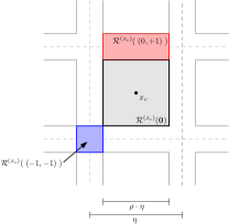
Figure 1: Illustration of $\mathcal{R}^{(x_{c})}$ notation for $X\subset\mathbb{R}^{2}$. For $x_{c}$ as labeled, the regions $\mathcal{R}^{(x_{c})}((-1,-1))$, $\mathcal{R}^{(x_{c})}((0,+1))$ and $\mathcal{R}^{(x_{c})}(\mathbf{0})$ are shown in blue, red and light gray, respectively.

The first step is to show that $\Upsilon_{\negthinspace\text{\tiny CPWA}}$ can be extended from the constant-valued region, $\mathcal{R}^{(x_{c})}(\mathbf{0})$, to each of its neighbors, $\mathcal{R}^{(x_{c})}(\iota)$, in a consistent way as a CPWA. To do this, first note that $\mathcal{R}^{(x_{c})}(\mathbf{0})$ has $2^{n}$ neighboring regions with indices $\iota^{\prime}\in\{-1,+1\}^{n}$, and each of these regions intersects a different $\mathcal{R}^{(x_{c}^{\prime})}(\mathbf{0})$ for $x_{c}^{\prime}\in\mathcal{N}(x_{c})$ at each corner, but is otherwise disjoint from them. Thus, Lemma 3 can be used to define a CPWA on each such $\mathcal{R}^{(x_{c})}(\iota^{\prime})$ in a way that is consistent with the definition of $\Upsilon_{\negthinspace\text{\tiny CPWA}}$ on the $\mathcal{R}^{(x_{c}^{\prime})}(\mathbf{0})$. These definitions are also consistent with each other, since these regions are disjoint. Moreover, this procedure yields the same extension when started from $x_{c}^{\prime}\in\mathcal{N}(x_{c})$ instead of $x_{c}$ (by the symmetric way that Lemma 3 is proved). Thus, it remains only to define $\Upsilon_{\negthinspace\text{\tiny CPWA}}$ on regions with indices of the form $\iota^{\prime\prime}\in\{-1,0,+1\}^{n}\backslash\{-1,+1\}^{n}\cup\{\mathbf{0}\}$. However, each such $\mathcal{R}^{(x_{c})}(\iota^{\prime\prime})$ intersects $2^{n-\text{dim}(\iota^{\prime\prime})}$ regions with indices of the form $\iota^{\prime}\in\{-1,+1\}^{n}$, and each of those intersections is a $\text{dim}(\iota^{\prime\prime})$ face of the corresponding $\mathcal{R}^{(x_{c})}(\iota^{\prime})$. But on each such $\text{dim}(\iota^{\prime\prime})$ face, $\Upsilon_{\negthinspace\text{\tiny CPWA}}$ is defined and agrees with $\Gamma_{\text{dim}(\iota^{\prime\prime})}$ from the construction in Lemma 3. Finally, since $\Gamma_{\text{dim}(\iota^{\prime\prime})}$ (and hence $\Upsilon_{\negthinspace\text{\tiny CPWA}}$) is identical up to isomorphism on each of these $\text{dim}(\iota^{\prime\prime})$ faces, $\Upsilon_{\negthinspace\text{\tiny CPWA}}$ can be extended on to $\mathcal{R}^{(x_{c})}(\iota^{\prime\prime})$ by isomorphism between the $\text{dim}(\iota^{\prime\prime})$ nonzero indices, and $\Upsilon_{\negthinspace\text{\tiny CPWA}}$ as defined on one of the $\text{dim}(\iota^{\prime\prime})$ faces of $\mathcal{R}^{(x_{c})}(\iota^{\prime})$. Finally, the symmetry of this procedure and Lemma 3 ensures that this assignment will be consistent when starting from some $x_{c}^{\prime}\in\mathcal{N}(x_{c})$ instead of $x_{c}$.

Next, we show that for this $\Upsilon_{\negthinspace\text{\tiny CPWA}}$, $\lVert\Upsilon_{\negthinspace\text{\tiny CPWA}}-\Psi\rVert\leq\mu/3$. This largely follows from the interpolation property proven in Lemma 3. In particular, on some $\mathcal{R}^{(x_{c})}(\iota)$, $\Upsilon_{\negthinspace\text{\tiny CPWA}}$ takes exactly the same values as some $\Gamma_{\text{dim}(\iota)}$ constructed according to Lemma 3, where the interpolation happens between $\text{dim}(\iota)$ points in $V\triangleq\{\Psi(x_{c}^{\prime})|x_{c}^{\prime}\in\mathcal{N}(x_{c})\cup\{x_{c}\}\}$. Thus,

$$\forall x\in\mathcal{R}^{(x_{c})}(\iota)\quad\min_{y\in V}\Psi(y)\leq\Upsilon_{\negthinspace\text{\tiny CPWA}}(x)\leq\max_{y\in V}\Psi(y).$$ (49)

Let $x\in\mathcal{R}^{(x_{c})}(\iota)$ be fixed temporarily, and suppose that $\Upsilon_{\negthinspace\text{\tiny CPWA}}(x)-\Psi(x)\geq 0$ and $\max_{y\in V}\Psi(y)-\Psi(x)\geq 0$. Then:

$$|\Upsilon_{\negthinspace\text{\tiny CPWA}}(x)-\Psi(x)|=\Upsilon_{\negthinspace\text{\tiny CPWA}}(x)-\Psi(x)\\ \leq\max_{y\in V}\Psi(y)-\Psi(x)=|\max_{y\in V}\Psi(y)-\Psi(x)|\leq\frac{\mu}{3}$$ (50)

where the last inequality follows from our choice of $\eta$ from Proposition 1, since $|y-x|\leq 2\eta$ for all $y\in V$. The other cases can be considered as necessary, and they lead to the same conclusion. Hence, we conclude $\lVert\Upsilon_{\negthinspace\text{\tiny CPWA}}-\Psi\rVert_{\infty}\leq\mu/3$, since our choice of center $x_{c}$ and $\iota$ was arbitrary.

Now we just need to (over)-count the number of linear regions needed in the extension $\Upsilon_{\negthinspace\text{\tiny CPWA}}$. This too will follow from the construction in Lemma 3. Note that on each $\mathcal{R}^{(x_{c})}(\iota)$, $\Upsilon_{\negthinspace\text{\tiny CPWA}}$ has the same number of linear regions as some $\Gamma_{\text{dim}(\iota)}$ that was constructed by Lemma 3, which by the same lemma has $2^{\text{dim}(\iota)-1}\cdot\text{dim}(\iota)!$ regions. Thus, we count at most:

$$\sum_{k=1}^{n}{n\choose k}\cdot 2^{k}\cdot 2^{k-1}\cdot k!=n!\cdot\sum_{k=1}^{n}\frac{2^{2k-1}}{(n-k)!}$$ (51)

linear regions. Finally, since we need this many regions for the neighboring regions of a single grid square, we obtain an upper bound for the total number of regions by multiplying (51) by the number of grid squares in the partition, $(\tfrac{\text{ext}(X)}{\eta})^{n}$ (then by the $m$, in the multi-dimensional output case). ∎

VII Numerical Results

Figure 2: States and inputs of the inverted pendulum with initial condition $[0.7,0.5]^{T}$.

Figure 3: States and inputs of the inverted pendulum with initial condition $[-0.4,1.0]^{T}$

We illustrate the results in this paper on an inverted pendulum described by the following model:

$$f(x_{1},x_{2},u)=\left[\begin{matrix}x_{2}&\frac{g}{l}\text{sin}(x_{1})-\frac{h}{ml^{2}}x_{2}+\frac{1}{ml}\text{cos}(x_{1})u\end{matrix}\right]^{\text{T}},$$

where $x_{1}$ is the angular position, $x_{2}$ is the angular velocity, and control input $u$ is the torque applied on the point mass. The parameters are the rod mass, $m$; the rod length, $l$; the (dimensionless) coefficient of rotational friction, $h$; and the acceleration due to gravity, $g$. For the purposes of our experiments, we considered a subset of the state/control space specified by: $x_{1}\in[-1,1]$, $x_{2}\in[-1,1]$ and $u\in[-6,6]$. Furthermore, we considered model parameters: $m=0.5$ kg; $l=0.5$ m; $h=2$; and $g=9.8$ N/kg. Then for different choices of the design parameters $\mu$, we obtained the following table of sizes, $N$, for the corresponding TLL-NN architecture; also shown are the corresponding $\tau$, $\eta$ and the $\delta$ that are required for the specification satisfaction.

$\mu$	$\delta$	$\tau$	$\eta$	$N$
0.35	0.8694	0.0098	0.583	235
0.3	0.5287	0.0083	0.5	320
0.25	0.3039	0.0069	0.417	460
0.2	0.1610	0.0056	0.334	720
0.15	0.0749	0.0042	0.25	1280
0.1	0.0275	0.0028	0.167	2880

In the sequel, we will show the control performance of a TLL-NN architecture with 400 local linear region. While there are a number of techniques that can be used to train the resulting NN, for simplicity, we utilize Imitation learning where the NN is trained in a supervised fashion from data collected from an expert controller. In particular, we designed an expert controller that stabilizes the inverted pendulum; we used Pessoa [14] to design our expert using the parameter values specified above. In particular, we tasked Pessoa to design a zero-order-hold controller that stabilizes the inverted pendulum in a subset $X_{\text{spec}}=[-1,1]\negthinspace\times\negthinspace[-0.5,0.5]$: i.e. the controller should transfer the state of the system to this specified set and keep it there for all time thereafter. From this expert controller, we collected 8400 data points of state-action pairs; this data was obtained by uniformly sampling the state space. We then used Keras [15] to train the TLL NN using this data. Finally, we simulated the motion of the inverted pendulum using this TLL NN controller. Shown in Fig. 2 and Fig. 3 are the state and control trajectories for this controller starting from initial state $[0.7,0.5]$ and $[-0.4,1]$, respectively. In both, the TLL controller met the same specification used to design the expert.

Appendix A Proofs

A-A Proof of Proposition 1

Proof.

Choose $\eta=\eta(\mu)\leq\frac{\mu}{2\cdot 3\cdot K_{\text{cont}}}$ and use Lipschitz continuity of $\Psi$. ∎

A-B Proof of Proposition 2

Proof.

Let $\mathcal{K}$ be the bound on $f$ as stated in Definition 1. Then by (4) we have

$$\lVert x-\zeta_{x\Upsilon}(t)\rVert =\left\lVert\int_{0}^{t}f(\zeta_{x\Upsilon}(\sigma),\Upsilon(\zeta_{x\Upsilon}(\sigma)))d\sigma\right\rVert$$ (52)

$$\leq\int_{0}^{t}\left\lVert f(\zeta_{x\Upsilon}(\sigma),\Upsilon(\zeta_{x\Upsilon}(\sigma)))\right\rVert d\sigma$$ (53)

$$\leq\int_{0}^{t}\mathcal{K}d\sigma=\mathcal{K}t.$$ (54)

Hence, choose $\tau=\tau(\mu)\leq\frac{\eta(\mu)}{\mathcal{K}}$ and the conclusion follows. ∎

A-C Proof of Proposition 3

Proof.

By the triangle inequality, we have:

$$\lVert\Upsilon(\zeta_{x\Upsilon}(t))-\Psi(\zeta_{x\Psi}(t))\rVert$$

$$\quad=\lVert\Upsilon(\zeta_{x\Upsilon}(t))-\Psi(\zeta_{x\Upsilon}(t))+\Psi(\zeta_{x\Upsilon}(t))-\Psi(\zeta_{x\Psi}(t))\rVert$$

$$\quad=\lVert\Upsilon(\zeta_{x\Upsilon}(t))-\Psi^{\prime}(\zeta_{x\Upsilon}(t))+$$

$$\qquad\qquad\Psi(\zeta_{x\Upsilon}(t))-\Psi(x)+\Psi(x)-\Psi(\zeta_{x\Psi}(t))\rVert$$

$$\quad\leq\lVert\Upsilon(\zeta_{x\Upsilon}(t))-\Psi(\zeta_{x\Upsilon}(t))\rVert+\lVert\Psi(\zeta_{x\Upsilon}(t))-\Psi(x)\rVert+$$

$$\qquad\qquad\lVert\Psi(x)-\Psi(\zeta_{x\Psi}(t))\rVert.$$ (55)

The first term in (60) is bounded by $\lVert\Upsilon-\Psi\rVert_{\infty}$. Now consider the second term. By Proposition 2, $\lVert\zeta_{x\Upsilon}(t)-x\rVert\leq\eta$; thus, by Proposition 1 we conclude that $\lVert\Psi(\zeta_{x\Upsilon}(t))-\Psi(x)\rVert\leq\mu/3$. The final term is likewise bounded by $\mu/3$ for the same reasons. Thus, the conclusion follows. ∎

A-D Proof of Proposition 4

Proof.

By definition and the properties of the integral, we have:

$$\lVert\zeta_{x\Upsilon}(t)-\zeta_{x\Psi}(t)\rVert$$

$$=\lVert\int_{0}^{t}f(\zeta_{x\Upsilon}(\sigma),\Upsilon(\zeta_{x\Upsilon}(\sigma)))-f(\zeta_{x\Psi}(t),\Psi(\zeta_{x\Psi}(t)))d\sigma\rVert$$

$$\leq\int_{0}^{t}\lVert f(\zeta_{x\Upsilon}(\sigma),\Upsilon(\zeta_{x\Upsilon}(\sigma)))-f(\zeta_{x\Psi}(t),\Psi^{\prime}(\zeta_{x\Psi}(t)))\rVert d\sigma$$

$$\leq\int_{0}^{t}K_{x}\lVert\zeta_{x\Upsilon}(\sigma)-\zeta_{x\Psi}(\sigma)\rVert$$

$$\qquad\qquad+K_{u}\lVert\Upsilon(\zeta_{x\Upsilon}(\sigma))-\Psi(\zeta_{x\Psi}(\sigma))\rVert d\sigma$$

$$\leq\int_{0}^{t}K_{x}\lVert\zeta_{x\Upsilon}(\sigma)-\zeta_{x\Psi}(\sigma)\rVert+K_{u}\cdot\kappa~{}d\sigma.$$ (56)

The claimed bound now follows directly from the Grönwall Inequality [8]. ∎

A-E Proof of Theorem 2

Proof.

By Lemma 4, there is a CPWA, $\Upsilon_{\negthinspace\text{\tiny CPWA}}$ that meets the assumptions of Lemma 2, and whose number of linear regions is upper-bounded by the quantity in (44). Thus, we are done if we can find a TLL NN architecture to implement the CPWA $\Upsilon_{\negthinspace\text{\tiny CPWA}}$. But by [7, Theorem 2], just such an architecture can be specified directly by the number of linear regions needed (as in (44)). This completes the proof. ∎

Appendix B Proofs

B-A Proof of Proposition 1

Proof.

Choose $\eta=\eta(\mu)\leq\frac{\mu}{2\cdot 3\cdot K_{\text{cont}}}$ and use Lipschitz continuity of $\Psi$. ∎

B-B Proof of Proposition 2

Proof.

Let $\mathcal{K}$ be the bound on $f$ as stated in Definition 1. Then by (4) we have

$$\lVert x-\zeta_{x\Upsilon}(t)\rVert =\left\lVert\int_{0}^{t}f(\zeta_{x\Upsilon}(\sigma),\Upsilon(\zeta_{x\Upsilon}(\sigma)))d\sigma\right\rVert$$ (57)

$$\leq\int_{0}^{t}\left\lVert f(\zeta_{x\Upsilon}(\sigma),\Upsilon(\zeta_{x\Upsilon}(\sigma)))\right\rVert d\sigma$$ (58)

$$\leq\int_{0}^{t}\mathcal{K}d\sigma=\mathcal{K}t.$$ (59)

Hence, choose $\tau=\tau(\mu)\leq\frac{\eta(\mu)}{\mathcal{K}}$ and the conclusion follows. ∎

B-C Proof of Proposition 3

Proof.

By the triangle inequality, we have:

$$\lVert\Upsilon(\zeta_{x\Upsilon}(t))-\Psi(\zeta_{x\Psi}(t))\rVert$$

$$\quad=\lVert\Upsilon(\zeta_{x\Upsilon}(t))-\Psi(\zeta_{x\Upsilon}(t))+\Psi(\zeta_{x\Upsilon}(t))-\Psi(\zeta_{x\Psi}(t))\rVert$$

$$\quad=\lVert\Upsilon(\zeta_{x\Upsilon}(t))-\Psi^{\prime}(\zeta_{x\Upsilon}(t))+$$

$$\qquad\qquad\Psi(\zeta_{x\Upsilon}(t))-\Psi(x)+\Psi(x)-\Psi(\zeta_{x\Psi}(t))\rVert$$

$$\quad\leq\lVert\Upsilon(\zeta_{x\Upsilon}(t))-\Psi(\zeta_{x\Upsilon}(t))\rVert+\lVert\Psi(\zeta_{x\Upsilon}(t))-\Psi(x)\rVert+$$

$$\qquad\qquad\lVert\Psi(x)-\Psi(\zeta_{x\Psi}(t))\rVert.$$ (60)

The first term in (60) is bounded by $\lVert\Upsilon-\Psi\rVert_{\infty}$. Now consider the second term. By Proposition 2, $\lVert\zeta_{x\Upsilon}(t)-x\rVert\leq\eta$; thus, by Proposition 1 we conclude that $\lVert\Psi(\zeta_{x\Upsilon}(t))-\Psi(x)\rVert\leq\mu/3$. The final term is likewise bounded by $\mu/3$ for the same reasons. Thus, the conclusion follows. ∎

B-D Proof of Proposition 4

Proof.

By definition and the properties of the integral, we have:

$$\lVert\zeta_{x\Upsilon}(t)-\zeta_{x\Psi}(t)\rVert$$

$$=\lVert\int_{0}^{t}f(\zeta_{x\Upsilon}(\sigma),\Upsilon(\zeta_{x\Upsilon}(\sigma)))-f(\zeta_{x\Psi}(t),\Psi(\zeta_{x\Psi}(t)))d\sigma\rVert$$

$$\leq\int_{0}^{t}\lVert f(\zeta_{x\Upsilon}(\sigma),\Upsilon(\zeta_{x\Upsilon}(\sigma)))-f(\zeta_{x\Psi}(t),\Psi^{\prime}(\zeta_{x\Psi}(t)))\rVert d\sigma$$

$$\leq\int_{0}^{t}K_{x}\lVert\zeta_{x\Upsilon}(\sigma)-\zeta_{x\Psi}(\sigma)\rVert$$

$$\qquad\qquad+K_{u}\lVert\Upsilon(\zeta_{x\Upsilon}(\sigma))-\Psi(\zeta_{x\Psi}(\sigma))\rVert d\sigma$$

$$\leq\int_{0}^{t}K_{x}\lVert\zeta_{x\Upsilon}(\sigma)-\zeta_{x\Psi}(\sigma)\rVert+K_{u}\cdot\kappa~{}d\sigma.$$ (61)

The claimed bound now follows directly from the Grönwall Inequality [8]. ∎

B-E Proof of Theorem 2

Proof.

By Lemma 4, there is a CPWA, $\Upsilon_{\negthinspace\text{\tiny CPWA}}$ that meets the assumptions of Lemma 2, and whose number of linear regions is upper-bounded by the quantity in (44). Thus, we are done if we can find a TLL NN architecture to implement the CPWA $\Upsilon_{\negthinspace\text{\tiny CPWA}}$. But by [7, Theorem 2], just such an architecture can be specified directly by the number of linear regions needed (as in (44)). This completes the proof. ∎

References

- [1] M. Bojarski, D. Del Testa, D. Dworakowski, B. Firner, B. Flepp, P. Goyal, L. D. Jackel, M. Monfort, U. Muller, J. Zhang, et al., “End to end learning for self-driving cars,” arXiv:1604.07316, 2016.
- [2] F. Pedregosa, “Hyperparameter optimization with approximate gradient,” arXiv:1602.02355, 2016.
- [3] J. Bergstra and Y. Bengio, “Random search for hyper-parameter optimization,” Journal of Machine Learning Research, vol. 13, no. Feb, pp. 281–305, 2012.
- [4] S. Paul, V. Kurin, and S. Whiteson, “Fast efficient hyperparameter tuning for policy gradients,” arXiv:1902.06583, 2019.
- [5] B. Baker, O. Gupta, N. Naik, and R. Raskar, “Designing neural network architectures using reinforcement learning,” arXiv:1611.02167, 2016.
- [6] Y. Quanming, W. Mengshuo, J. E. Hugo, G. Isabelle, H. Yi-Qi, L. Yu-Feng, T. Wei-Wei, Y. Qiang, and Y. Yang, “Taking human out of learning applications: A survey on automated machine learning,” arXiv:1810.13306, 2018.
- [7] J. Ferlez and Y. Shoukry, “AReN: Assured ReLU NN Architecture for Model Predictive Control of LTI Systems,” in Hybrid Systems: Computation and Control 2020 (HSCC’20), ACM, New York, 2020.
- [8] H. K. Khalil, Nonlinear Systems. Pearson, Third ed., 2001.
- [9] M. Zamani, G. Pola, M. Mazo, and P. Tabuada, “Symbolic Models for Nonlinear Control Systems Without Stability Assumptions,” IEEE Transactions on Automatic Control, vol. 57, no. 7, 2012.
- [10] V. Kurtz, P. M. Wensing, and H. Lin, “Robust Approximate Simulation for Hierarchical Control of Linear Systems under Disturbances,” 2020.
- [11] K. Mallik, A.-K. Schmuck, S. Soudjani, and R. Majumdar, “Compositional Synthesis of Finite-State Abstractions,” IEEE Transactions on Automatic Control, vol. 64, no. 6, pp. 2629–2636, 2019.
- [12] G. Pola, A. Girard, and P. Tabuada, “Approximately bisimilar symbolic models for nonlinear control systems,” Automatica, vol. 44, no. 10, pp. 2508–2516, 2008.
- [13] P. Tabuada, Verification and Control of Hybrid Systems: A Symbolic Approach. Springer US, 2009.
- [14] M. Mazo, A. Davitian, and P. Tabuada, “PESSOA: A tool for embedded controller synthesis,” in Proceedings of the 22nd International Conference on Computer Aided Verification, CAV’10, pp. 566–569, Springer-Verlag, 2010.
- [15] F. Chollet et al., “Keras.” https://keras.io, 2015.