A New Model For Including Galactic Winds in Simulations of Galaxy Formation I: Introducing the Physically Evolved Winds (PhEW) Model

Abstract

The propagation and evolution of cold galactic winds in galactic haloes is crucial to galaxy formation models. However, modelling of this process in hydrodynamic simulations of galaxy formation is over-simplified owing to a lack of numerical resolution and often neglects critical physical processes such as hydrodynamic instabilities and thermal conduction. We propose an analytic model, Physically Evolved Winds (PhEW), that calculates the evolution of individual clouds moving supersonically through a uniform ambient medium. Our model reproduces predictions from very high resolution cloud-crushing simulations that include isotropic thermal conduction over a wide range of physical conditions. We discuss the implementation of this model into cosmological hydrodynamic simulations of galaxy formation as a sub-grid prescription to model galactic winds more robustly both physically and numerically.

1 Introduction

Many lines of evidence imply that galactic winds are a critical element of the physics of galaxy formation. Most directly, observations reveal ubiquitous outflows from star-forming galaxies at $z\sim 2$ (Steidel et al., 2010) and from starburst or post-starburst galaxies at low redshift (Veilleux et al., 2020). Semi-analytic models and hydrodynamic cosmological simulations that do not incorporate strong outflows predict galaxies that are too massive and too metal-rich (e.g., White & Frenk 1991; Benson et al. 2003). UV absorption studies demonstrate the existence of a cool ($T\sim 10^{4}\,{\rm K}$), enriched circumgalactic medium (CGM) with a mass and metal content comparable to or even exceeding that of the galaxy’s stellar component (e.g. Tumlinson et al. 2011; Werk et al. 2014; Peeples et al. 2014; Tumlinson et al. 2017). X-ray studies reveal a hot, metal-enriched CGM around elliptical galaxies (e.g. Anderson et al., 2013), some massive spirals (e.g. Bogdán et al. 2013; Bogdán et al. 2017), and the Milky Way (e.g. Gupta et al. 2012; Gupta et al. 2017). Hydrodynamic simulations play a crucial role in interpreting these observations, but the physical processes that govern the launch and propagation of winds are uncertain and may occur on scales well below the resolution limit of the simulations. In this paper we describe a “sub-grid” approach to modelling wind propagation, one that adopts a phenomenological description of cold cloud evolution informed by high resolution numerical studies.

Many mechanisms have been proposed for launching galactic winds, including radiation pressure from young stars, energy and momentum injection from stellar winds and supernovae, and cosmic ray pressure gradients. Different mechanisms may dominate in different situations, and in some cases the combination of two or more mechanisms may be crucial (Hopkins et al., 2012). In high mass galaxies, observational and theoretical evidence suggests that feedback from accreting supermassive black holes (AGN feedback) becomes the dominant driver of outflows. Very high resolution simulations, some from cosmological initial conditions, others of isolated disks or sections of the interstellar medium (ISM), are beginning to provide insights into the ways that these mechanisms launch outflows (e.g., Hopkins et al. 2012; Girichidis et al. 2016; Tanner et al. 2016; Fielding et al. 2017; Kim & Ostriker 2017; Li et al. 2017; Schneider et al. 2018). Observations frequently reveal the co-existence of molecular gas, neutral atomic gas, cool ionised gas, and hot X-ray emitting gas in the same outflows (Veilleux et al., 2020), with the cold and cool phases often dominating the total mass. Accurately modelling the interactions among these multiple phases is a critical challenge. The acceleration of large amounts of cold/cool gas to highly supersonic velocities is a particular puzzle, with possible mechanisms including radiation pressure on cold clouds (Murray et al., 2005), entrainment of cold gas in a hot wind (Scannapieco & Brüggen, 2015; Schneider & Robertson, 2017), the formation of the cold/cool phases out of the hot flow by radiative cooling (Thompson et al., 2016; Schneider et al., 2018), or many mechanisms combined (Yu et al., 2020).

Our focus in this paper is not the wind launch process itself but the evolution of winds after ejection from the galaxy and their interaction with the CGM. Most hydrodynamic simulations of cosmological volumes — tens of Mpc on a side, containing many galaxies — adopt a phenomenological model in which wind particles are launched stochastically from each star-forming galaxy at rates and velocities motivated by analytic models or by pressure gradients induced with tuned prescriptions of energy or momentum injection. Examples include our own group’s simulations (e.g., Oppenheimer & Davé 2006; Davé et al. 2013, 2019; Huang et al. 2020) and the Illustris (Vogelsberger et al., 2013) and Illustris TNG (Pillepich et al., 2018a) simulations. Other groups add the feedback energy as thermal energy, e.g. Stinson et al. (2006), EAGLE (Schaye et al., 2015) and FIRE (Hopkins et al., 2012), and allow the winds to develop as a result. Cosmological volume simulations enable statistical comparisons to the observed evolution of galaxy masses, sizes, star formation rates, and gas content (e.g., Oppenheimer et al. 2010; Pillepich et al. 2018b; Davé et al. 2019), and they have played an essential role in interpreting UV absorption observations of the CGM (e.g., Ford et al. 2013, 2016; Nelson et al. 2018). However, given the potential sensitivity of predictions to physical processes in the CGM below the resolution limit of the simulations, independent of how the winds are generated in the simulations, it is still unclear which empirical successes of the simulations are true successes and which failures are true failures. Simulations that deliberately amplify resolution in the CGM offer one route to examining the impact of resolution on predictions showing that some quantities can be significantly affected (e.g., Hummels et al. 2019; Peeples et al. 2019; van de Voort et al. 2019). Another approach to increase the resolution is to use “zoom” simulations to model one galaxy at a time (e.g. Governato et al., 2007; Hopkins et al., 2014; Wang et al., 2015; Grand et al., 2017). However, even these simulations do not resolve the tens of pc-scale structures suggested by some theoretical models of thermal instability (McCourt et al., 2018; Mandelker et al., 2019) and by estimates of cool-phase cloud sizes inferred from measured column densities and derived number densities (e.g., Pieri et al. 2014; Crighton et al. 2015; Stern et al. 2016). Furthermore, with current computational capabilities it is infeasible to maintain even kpc-scale resolution throughout volumes that are tens of Mpc on a side, and standard Lagrangian or mesh refinement schemes will not automatically resolve the regions of the CGM where gas phases interact. Physical processes in addition to radiative hydrodynamics, such as thermal conduction, viscosity and magnetic fields, may also have significant effects on cloud evolution (Marcolini et al., 2005; Orlando et al., 2005; Vieser & Hensler, 2007; McCourt et al., 2015; Brüggen & Scannapieco, 2016; Armillotta et al., 2016, 2017; Li et al., 2019), but they are rarely incorporated self-consistently in cosmological simulations.

In the approach proposed here, we eject wind particles as in previous simulations but follow their evolution and interaction with the ambient CGM using an analytic sub-grid model. We model the gas in each wind particle as a collection of cold clouds, and we calculate the exchange of mass, momentum, energy, and metals between these clouds and the surrounding CGM gas. A wind particle loses mass as it evolves, and it is dissolved when its mass falls below some threshold, or when its velocity and physical properties sufficiently resemble the surrounding gas, or when it rejoins a galaxy and contributes its remaining mass and metals to the ISM. This general method can be implemented in cosmological simulations that use smoothed particle hydrodynamics (SPH) or Eulerian or Lagrangian mesh codes. In future work we will present results from implementing this Phenomenologically Evolved Wind (PhEW) model in cosmological simulations with the GIZMO hydrodynamics code (Hopkins & Raives, 2016), employing the star formation and feedback recipes described by Davé et al. (2019) and the wind launch prescriptions described by Huang et al. (2020), which are themselves tuned to reproduce outflows in the FIRE simulations (Muratov et al., 2015). In this paper we present the wind model itself.

This model is based on results from very high resolution simulations of the “cloud-crushing problem,” which examine the evolution of an individual cold clouds moving supersonically relative to an ambient, hotter flow (see Banda-Barragán et al. 2019 for a recent compilation of such simulations). We concentrate in particular on the cloud-crushing simulations of Scannapieco & Brüggen (2015, hereafter SB15), which do not include thermal conduction, and the simulations of Brüggen & Scannapieco (2016, hereafter BS16), which do. These simulations model idealised situations with mass and spatial resolutions far higher than that achieved in any galaxy formation or cosmological hydrodynamic simulations. PhEW provides a method to transfer the lessons from these high resolution studies to a cosmological context. This method necessarily introduces new free parameters, the most important being the individual cold cloud mass and the strength of thermal conduction. However, traditional implementations of galactic winds in cosmological simulations implicitly introduce a non-physical “sub-grid” model that is governed by the numerics of the interaction between wind particles and the ambient gas with very different physical properties. The effects of this non-physical model (e.g., the degree to which cold gas remains cold) may be sensitive to the numerical resolution. PhEW replaces these numerically governed interactions with a model that is physical, approximate, makes specified and controllable assumptions, and should be less sensitive to numerical resolution.

The paper is organised as follows. In Section 2 we describe the set-up of the cloud-crushing problem and the various physical processes involved and also introduce the cloud-crushing simulations (BS16) that we use to develop the analytic model. In Section 3 we discuss different physical regimes of the problem and the dominant physics. In Section 4.1 we describe our analytic model and provide a detailed calculation of how physical properties of the cloud evolve with time. In Section 4.2 we summarise the key assumptions and approximations in the analytic model and discuss where they might break down. In Section 5 we compare our model predictions to simulation results from (BS16). In Section 6 we summarise the main results from the paper, describe how to implement the analytic model in cosmological simulations that use various hydrodynamic methods and discuss the implications of this model in galaxy formation.

2 The Cloud-Crushing Problem

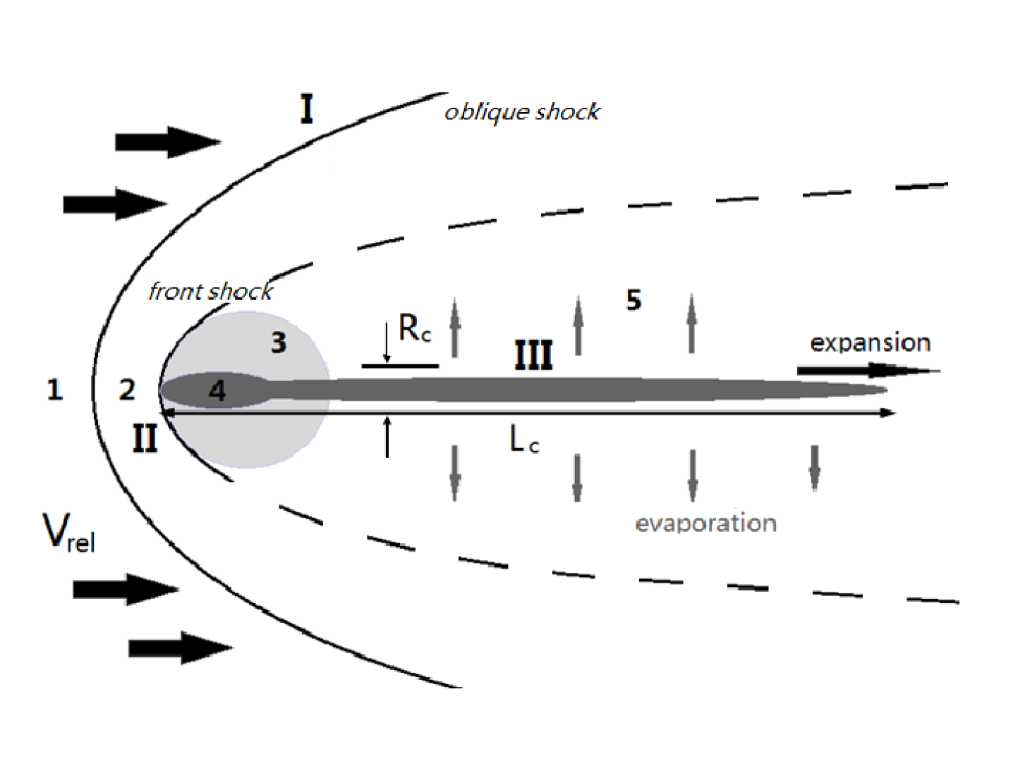
Figure 1: Cloud crushing problem set up. See text for description. Here region 2 represents only the gas that surrounds the head of the cloud. The transition region 5 between the oblique shock boundary I and the cloud boundary III appears broader than is likely in reality. The fluid properties within this region are determined by the combined effects of the oblique shock and the evaporative flow.

We set up the cloud-crushing problem as illustrated in Figure 1. An initially uniform, spherical cloud of mass $M_{\mathrm{c}}$, density $\rho_{3}$ and temperature $T_{3}$ is placed in an ambient medium of uniform density $\rho_{1}$ and temperature $T_{1}$ with a relative velocity $v_{\mathrm{rel}}$. The initial density contrast between the cloud and the ambient medium is $\chi_{0}\equiv\rho_{3}/\rho_{1}$.

At the beginning, the cloud is in thermal pressure equilibrium with the surrounding medium so that $\rho_{3}T_{3}=\rho_{1}T_{1}$. We let the cloud move relative to the ambient at a velocity $v_{\mathrm{rel}}$. Here we only study the cases where the cloud is moving supersonically as is typical in wind-CGM interactions, i.e., $\mathcal{M}_{1}\equiv v_{\mathrm{rel}}/c_{\mathrm{s,1}}>1$, where $c_{\mathrm{s,1}}$ is the isothermal sound speed of the ambient medium. The discontinuity in front of the cloud separates into a bow shock (region 2) that moves into the ambient medium and a cloud shock that advances into the cloud. We note the surface at the front of the bow shock with roman numeral I and the surface at the contact discontinuity with roman numeral II. We define the cloud-crushing time-scale as $\tau_{\mathrm{cc}}\equiv\chi_{0}^{1/2}(R_{\mathrm{c}}/v_{\mathrm{rel}})$ (SB15), where $R_{\mathrm{c}}$ is the initial radius of the cloud. It takes $\sim\tau_{\mathrm{cc}}$ for the cloud shock to sweep through the cloud, crushing it into a much higher density $\rho_{4}$ and pressure $P_{4}$ that is comparable to the pressure at the stagnation point $P_{\mathrm{II}}$. After the cloud shock, the cloud will re-expand preferentially in the under-pressured downstream direction. The ambient flow between the shock front I and the boundary of the cloud (III) is continuous and obeys Bernoulli’s equations.

In cloud-crushing simulations without thermal conduction, the clouds are vulnerable to hydrodynamic instabilities. For example, in many cases, perturbations grow at the cloud boundary III owing to the Kelvin-Helmholtz Instability (KHI), which eventually leads to the fragmentation and disruption of the cloud within a few $\tau_{\mathrm{cc}}$. Even in high Mach flows where the KHI tends to be suppressed, the cloud hardly survives beyond 30 $\tau_{\mathrm{cc}}$ (SB15).

Cloud-crushing simulations with thermal conduction suggest that efficient thermal conduction significantly affects cloud evolution (Orlando et al., 2005; Vieser & Hensler, 2007; Brüggen & Scannapieco, 2016; Armillotta et al., 2016, 2017; Li et al., 2019): First, the cloud evaporates when thermal conduction is sufficiently strong. In many such simulations, cloud evaporation is the leading cause of mass loss. Rapid evaporation sometimes destroys the cloud much sooner than without conduction. Second, the evaporated material streaming away from the cloud creates a conduction zone where the pressure $P_{\mathrm{ev}}$ at the cloud surface III is larger than the thermal pressure (Cowie & McKee, 1977, hereafter CM77). This helps to confine the cloud and prevent it from fragmentation caused by KHI. In BS16, the clouds often display a needle-like morphology as illustrated in Figure 1, with radius $R_{\mathrm{c}}$ and length $L_{\mathrm{c}}$, instead of breaking up into small clumps, which occurs when there is no conduction (SB15). Third, the deceleration rate of the cloud from ram pressure $P_{\mathrm{II}}$ is reduced because its cross section ($\pi R_{\mathrm{c}}^{2}$) shrinks owing to the additional vapour pressure. Fourth, the jump conditions at the bow shock must be modified from the Rankine-Hugoniot formula owing to conductive heat flux cross the shock discontinuity. This has a significant effect on the properties of the post-shock gas in region 2 and the ambient flow in region 5.

Since the cloud evolution depends heavily on whether or not thermal conduction is efficient, we will treat these two regimes separately. The heat advection rate from thermal conduction is very sensitive to the temperature of the hot phase. Galaxy formation theory suggests that, in the real Universe, galactic haloes separate into cold haloes with gas at the photoionisation equilibrium temperature of $\sim 10^{4}\,\mathrm{K}$ and hot haloes at the virial temperatures over $10^{6}\,\mathrm{K}$(Kereš et al., 2005, 2009; Dekel et al., 2009). Thermal conduction is, therefore, expected to be only important in hot haloes.

Magnetic fields can suppress thermal conduction significantly even if they are not dynamically important (Li et al., 2019). However, the strength of magnetic fields in galactic haloes is poorly constrained and the effects of tangled magnetic fields on thermal conduction is uncertain. Therefore, we do not explicitly model magnetic fields in this work. Instead, we use a free parameter to control the overall efficiency of thermal conduction.

To implement this process as a sub-grid model into cosmological simulations, we will focus on explicitly calculating the rate of deceleration and the mass loss rate of the cloud. The deceleration is caused by the ram pressure $P_{\mathrm{II}}$ in front of the cloud and depends on the cross section $\pi R_{\mathrm{c}}^{2}$ and the mass of the cloud $M_{\mathrm{c}}$. Therefore, the deceleration rate is largely determined by the properties of the bow shock and of the compressed cloud, though both change drastically when one includes thermal conduction.

The mass loss is primarily caused by hydrodynamic instabilities or thermal conduction or a combination of these two, but their calculation is more complicated. When thermal conduction is inefficient, the cloud loses its mass primarily from KHI and the expansion in the downstream direction after the cloud shock. The lifetime of the cloud is characterised by the Kelvin-Helmholtz time-scale $\tau_{\mathrm{KH}}$, which will be described in Section 3.4 based on the numerical results from SB15. In the rest of the paper, we will mostly focus on the regimes where thermal conduction and evaporation are important. We develop a model for this regime based on the results from BS16.

Table 1: Numerical simulations from BS16 and their parameters.

Name	$M_{\mathrm{c}}/M_{\odot}$	$v_{\mathrm{rel}}[\mathrm{kms^{-1}}]$	$R_{\mathrm{c}}[\mathrm{pc}]$	$n_{\mathrm{c}}[\mathrm{cm}^{-3}]$	$n_{\mathrm{a}}[\mathrm{cm}^{-3}]$	$T_{\mathrm{a}}[\mathrm{K}]$	$N_{\mathrm{c}}[\mathrm{cm}^{-2}]$	$\tau_{\mathrm{cc}}[\mathrm{Myr}]$
$\chi 300v1000$	$6.7\times 10^{4}$	$1000$	$100$	$1.0$	$3.3\times 10^{-3}$	$3\times 10^{6}$	$1.5\times 10^{20}$	$1.69$
$\chi 300v1700$	$6.7\times 10^{4}$	$1700$	$100$	$1.0$	$3.3\times 10^{-3}$	$3\times 10^{6}$	$1.5\times 10^{20}$	$0.996$
$\chi 1000v1700$	$6.7\times 10^{4}$	$1700$	$100$	$1.0$	$1.0\times 10^{-3}$	$10\times 10^{6}$	$1.5\times 10^{20}$	$1.82$
$\chi 3000v3000$	$6.7\times 10^{4}$	$3000$	$100$	$1.0$	$1.0\times 10^{-3}$	$3\times 10^{6}$	$1.5\times 10^{20}$	$1.79$
$\chi 300v3000$	$6.7\times 10^{4}$	$3000$	$100$	$1.0$	$0.33\times 10^{-3}$	$3\times 10^{6}$	$1.5\times 10^{20}$	$0.565$
$\chi 300v3000b$	$6.7\times 10^{4}$	$3000$	$46.4$	$10.0$	$3.3\times 10^{-3}$	$3\times 10^{6}$	$1.5\times 10^{21}$	$0.262$
$\chi 1000v480$	$6.7\times 10^{4}$	$480$	$100$	$1.0$	$1.0\times 10^{-3}$	$10\times 10^{6}$	$1.5\times 10^{20}$	$6.45$
$\chi 3000v860$	$6.7\times 10^{4}$	$860$	$100$	$1.0$	$0.33\times 10^{-3}$	$30\times 10^{6}$	$1.5\times 10^{20}$	$6.23$

Both SB15 and BS16 study cloud evolution using a set of cloud-crushing simulations with varying flow parameters. BS16 includes isotropic thermal conduction at the Spitzer rate $f_{\mathrm{s}}=1$. Some of these simulations and their parameters are listed in Table 1. The simulations are named after the initial density contrast $\chi$ and the relative velocity $v_{\mathrm{rel}}$. These simulations explore a variety of physical conditions that are typical of interactions between winds and the hot CGM, with the ambient temperatures ranging from $3\times 10^{6}\,\mathrm{K}$ to $3\times 10^{7}\,\mathrm{K}$ and the initial Mach number ranging from 1.0 to 11.4. We also ran two additional simulations, $\chi 300v1700c5$ and $\chi 300v1700c20$ to explore the effects of reduced thermal conduction. They have the same initial conditions as $\chi 300v1700$, but have only 1/5 and 1/20 of the original strength of thermal conduction, respectively.

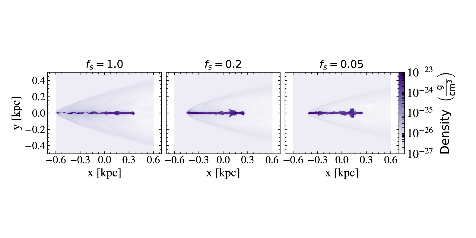
Figure 2: From left to right: Density slices from the $\chi 300v1700$, $\chi 300v1700c5$ and $\chi 300v1700c20$ simulations at $\sim 8.5$ Myrs. These simulations have different $f_{\mathrm{s}}$ values as indicated in the figure. At this time, the cloud in the $\chi 300v1700$ simulation has evaporated nearly 50% of its mass, considerably more than in the other two simulations. The cloud in the $\chi 300v1700c20$ simulation is still able to resist hydrodynamic instabilities even though thermal conduction is only 1/20 of the Spitzer value there.

3 Physical Processes

In this section, we review the physical processes that are critical to the evolution of the cloud in the cloud-crushing problem and describe how to calculate relevant properties of the cloud and the ambient medium during its evolution. In Section 3.1 we review some general formulae about thermal conduction. In Section 3.2 we find solutions to the bow shock and the cloud-crushing shock, with or without thermal conduction. In Section 3.3 we describe the morphology of the cloud after the cloud shock, the expansion of the cloud, and the internal structure of the cloud during the expansion. In Section 3.4 we discuss how clouds lose mass owing to the Kelvin-Helmholtz instability and how to determine whether or not thermal conduction suppresses the KHI. In Section 3.5 we propose an approximate model of estimating the mass loss rate from a cloud owing to conduction-driven evaporation. In Section 3.6, we discuss the effects of radiative cooling on our analytic model.

3.1 Classical and Saturated Conduction

Throughout this paper we do not consider the effect of magnetic fields and assume isotropic thermal conduction. Thermal conduction relies on electrons in the hot plasma exchanging kinetic energy with the electrons in the cold gas. In the hot plasma, the mean free path of an electron is $\lambda_{\mathrm{mfp}}\sim 1.65\times 10^{4}\ [\mathrm{cm}]\ T_{e}^{2}/n_{e}$, where $T_{e}$ and $n_{e}$ are the electron temperature and electron number density in the plasma. In this paper, we will assume that electrons and ions are always in thermal equilibrium and have the same temperature $T_{\mathrm{h}}=T_{e}=T_{i}$ in the plasma, where $T_{i}$ is the ion temperature. In the classical limit where the mean free path, $\lambda_{\mathrm{mfp}}$, is much smaller than the scale of the temperature gradient $L_{\mathrm{T}}$, thermal conduction leads to a heat flux

$$q_{\mathrm{class}}=-\kappa_{\mathrm{h}}\nabla T,$$ (1)

where $\kappa_{\mathrm{h}}$ is a function of the temperature and density in the hot medium:

$$\kappa_{\mathrm{h}}=6.1\times 10^{-7}T_{\mathrm{h}}^{5/2}\left(\frac{30}{\ln\Lambda_{\kappa}}\right)$$ (2)

and $\ln\Lambda_{\kappa}\equiv 29.7+\ln n_{e}^{-1/2}(T_{e}/10^{6}\,\mathrm{K})$ is the Coulomb logarithm that depends very weakly on $n_{e}$ and $T_{e}$. In this paper, we will always set $\ln\Lambda_{\kappa}=30$ for simplicity.

When $\lambda_{\mathrm{mfp}}\gg L_{\mathrm{T}}$, the cross sections of electron-electron collisions become too large for conduction to work in the classic limit. It reduces the efficiency of heat transfer to a saturated value (CM77):

$$q_{\mathrm{sat}}=0.4f_{\mathrm{s}}\left(\frac{2k_{\mathrm{B}}T_{e}}{\pi m_{e}}\right)^{1/2}n_{e}k_{\mathrm{B}}T_{e}\sim 1.715\times 10^{-11}n_{e}T_{e}^{3/2},$$ (3)

where $k_{\mathrm{B}}$ is the Boltzmann constant, $f_{\mathrm{s}}\leq 1$ is a free parameter that determines the overall efficiency of thermal conduction. $f_{\mathrm{s}}=1$ indicates thermal conduction at the Spitzer rate.

Similar to CM77, we define a saturation parameter $\sigma_{0}$ that distinguishes classical conduction and saturated conduction based on the flow parameters:

$$\sigma_{0}=\frac{2\kappa_{\mathrm{h}}T_{\mathrm{h}}}{25\rho_{h}c_{h}^{3}R_{\mathrm{c}}}=1.84\frac{\lambda_{h}}{L_{T}},$$ (4)

where $c_{h}$ is the isothermal sound speed of the hot medium, and $\lambda_{h}$ is the mean free path of the hot medium. Physically, $\sigma_{0}$ is the ratio between $q_{\mathrm{class}}$ and $q_{\mathrm{sat}}$. We use the classical heat flux when $\sigma_{0}<1$ and the saturated heat flux otherwise.

Thermal conduction at an interface between hot and cold gas could lead to evaporation of cold gas into the hot gas, as the cold gas near the interface gains energy from electron collision. In the classical limit, CM77 derive the evaporation time-scale for a spherical cloud of uniform density in an initially uniform, infinite hot medium as

$$\tau_{\mathrm{ev,class}}=\frac{25k_{\mathrm{B}}M_{\mathrm{c}}}{16\pi\mu m_{\mathrm{H}}\kappa f_{\mathrm{s}}R_{\mathrm{c}}},$$ (5)

where $\mu$ is the atomic weight and $m_{\mathrm{H}}$ is the mass of the hydrogen atom. The above equation can be written numerically as:

$$\tau_{\mathrm{ev,class}}=48.9\ [\mathrm{Myr}]\left[\left(\frac{n_{\mathrm{c}}}{1\,\mathrm{cm}^{-3}}\right)\left(\frac{R_{\mathrm{c}}}{10\,\mathrm{pc}}\right)^{2}\left(\frac{T_{\mathrm{h}}}{10^{6}\,\mathrm{K}}\right)^{-2.5}\right],$$ (6)

where $R_{\mathrm{c}}$ and $M_{\mathrm{c}}$ are the radius and mass of the spherical cloud, and $f_{\mathrm{s}}\leq 1$ is a constant factor that determines the strength of thermal conduction relative to the Spitzer value (Equation 1).

In the saturated limit ($\sigma_{0}>1$), the evaporation time-scale becomes (CM77):

$$\tau_{\mathrm{ev,sat}}=10.3\ [\mathrm{Myr}]\left(\frac{\chi}{10^{3}}\right)\left(\frac{R_{\mathrm{c}}}{10\,\mathrm{pc}}\right)\left(\frac{T_{\mathrm{h}}}{10^{6}\,\mathrm{K}}\right)^{-1/2}\sigma_{0}^{-3/8},$$ (7)

which is obtained from their equation 64 with the parameter $\phi_{\mathrm{s}}$ in the equation set to 1.0.

Note, however, that the above treatment of evaporation is only valid when the mean free path of hot electrons inside the cloud is much smaller than the cloud radius. Otherwise, hot electrons will be able to free stream through the cloud while at the same time heating the entire cloud through coulomb heating (Balbus & McKee, 1982). When the coulomb heating rate exceeds the radiative cooling rate, the cloud will puff up quickly and disintegrate shortly thereafter (Li et al., 2019). This only occurs for very small clouds in a very hot medium and puts a lower limit on the initial cloud size, which is a main parameter of our model. BS16 show that this quick disruption occurs when the initial column density of the cloud is smaller than $1.3\times 10^{18}\mathrm{cm}^{-2}(T_{1}/10^{7}\,\mathrm{K})^{2}$ and demonstrate in a test simulation that a cloud with an initial size of $R_{\mathrm{c}}=1\,\mathrm{pc}$ in a surrounding medium with $\chi=3000,T_{1}=10^{7}\,\mathrm{K}$, and $v_{\mathrm{rel}}=3000$ km s^-1indeed evaporates within $1\tau_{\mathrm{cc}}$. However, this lower limit is much below the physical conditions probed in BS16 in which we are interested in this paper.

The CM77 solution for conductive evaporation also assumes that radiative cooling is negligible. We will further discuss the effects of cooling on thermal conduction in Section 3.6.

3.2 The Bow Shock and the Cloud Shock

3.2.1 Without Thermal Conduction

In the non-conductive limit, we approximate the bow shock as adiabatic so that the physical conditions at the two sides of the shock (boundary I) are related by the Rankine-Hugoniot jump conditions (appendix B). In the post-shock gas (region 2), the flow is subsonic and is governed by the Bernoulli equations that relate post-shock quantities at boundary I to the fluid quantities at the stagnation point II. The pressure at the stagnation point and that in the shocked cloud (region 4) are the same ($P_{\mathrm{II}}=P_{4}$).

The thermal pressure of the pre-shock medium $P_{1}$ and the pressure at the stagnation point is, therefore, related by (McKee & Cowie, 1975):

$$\frac{P_{\mathrm{II}}}{P_{1}}=\frac{P_{\mathrm{II}}}{P_{I}}\frac{P_{I}}{P_{1}}=\left(\frac{\gamma+1}{2}\right)^{\frac{\gamma+1}{\gamma-1}}\left(\gamma-\frac{\gamma-1}{2\mathcal{M}_{1}^{2}}\right)^{-\frac{1}{\gamma-1}}\mathcal{M}_{1}^{2},$$ (8)

where $\mathcal{M}_{1}$ is the Mach number of the pre-shock gas in the velocity frame of the cloud:

$$\mathcal{M}_{1}\equiv\frac{v_{1}}{c_{\mathrm{s,1}}}$$ (9)

and $c_{\mathrm{s,1}}$ is the isothermal sound speed in the unshocked gas.

Equation 8 only applies in the supersonic case $\mathcal{M}_{1}>1$. Here $P_{\mathrm{II}}$ is also the ram pressure that is responsible for the deceleration of the cloud:

$$P_{\mathrm{ram}}\sim f_{\mathrm{ram}}(\mathcal{M}_{\mathrm{rel}})\rho_{\mathrm{a}}v_{\mathrm{rel}}^{2},$$ (10)

where $\mathcal{M}_{\mathrm{rel}}$ is the mach number of the ambient flow relative to the cloud, and the coefficient $f_{\mathrm{ram}}$ can be derived from Equation 8 with $P_{\mathrm{ram}}=P_{\mathrm{II}}$. It is of order unity and has a minimum value 0.5 when $\mathcal{M}_{\mathrm{rel}}=1$. For simplicity, we choose $f_{\mathrm{ram}}=0.5$ in this paper. Our results are not sensitive to this choice of $f_{\mathrm{ram}}$.

The cloud shock propagates at a speed $v_{s}$ that can be solved using the jump conditions at the cloud shock front. Assuming the cloud shock is isothermal, we approximate the shock speed according to the jump condition:

$$\frac{P_{\mathrm{II}}}{P_{3}}=\left(\frac{v_{s}}{c_{\mathrm{s,c}}}\right)^{2},$$ (11)

where $c_{\mathrm{s,c}}$ is the isothermal sound speed of the cloud. The shock speed is related to the cloud crushing time by $v_{s}\sim R_{\mathrm{c}}(t=0)/\tau_{\mathrm{cc}}$.

Therefore, by assuming an adiabatic bow shock and an isothermal cloud shock, we are able to solve for the post-shock properties of the cloud. The cloud is compressed within a few $\tau_{\mathrm{cc}}$ and accelerated to the shock speed $v_{s}$. The density inside the cloud is enhanced by a factor of $\rho_{4}/\rho_{3}\sim\chi^{-1}(v_{1}/c_{\mathrm{s,c}})^{2}$, making it over-pressured relative to its surroundings.

3.2.2 With Conduction

Including thermal conduction could significantly affect the bow shock as well as the cloud-crushing shock. Either in the regime of classical conduction, where $q\sim T^{2.5}$, or in the regime of saturated conduction, where $q\sim n_{e}T_{e}^{1.5}$, the heat flux $q$, the evaporation rate $\dot{m}$, and the vapour pressure $P_{\mathrm{ev}}$ are all very sensitive to the post-shock properties of the flow. Furthermore, the post-shock flow is no longer a constant flow determined by the Rankine-Hugoniot jump condition, but rather displays a time-dependent profile behind the main shock front. The picture of a radiative shock with electron thermal conduction has been extensively studied in the literature (Lacey, 1988; Borkowski et al., 1989). While these works focus on plane-parallel shocks driven by a supersonic flow in a single continuous medium, the cloud-crushing problem requires a self-consistent solution in a two-phase medium, i.e., hot ambient gas and a cool cloud.

Despite these complications, we extended the Borkowski et al. (1989) prescription for a conductive shock by including a non-negligible initial temperature. Inheriting their notation, we may solve for the modified Rankine-Hugoniot jump conditions (see appendix B for the derivation). The density and temperature ratio across the conductive shock front becomes:

$$x_{\mathrm{s}}\equiv\frac{\rho_{1}}{\rho_{2}}=\frac{5(1+\beta_{\mathrm{s}})-\sqrt{9+16\hat{q}_{\mathrm{s}}+5\beta_{\mathrm{s}}(5\beta_{\mathrm{s}}-6)}}{8}$$ (12)

and

$$\frac{T_{1}}{T_{2}}=\frac{\beta_{\mathrm{s}}}{(1+\beta_{\mathrm{s}}-x_{\mathrm{s}})x_{\mathrm{s}}}.$$ (13)

In the above equations, $\hat{q}_{\mathrm{s}}$ is a parameter that is explained in detail below, and $\beta_{\mathrm{s}}$ is defined as:

$$\beta_{\mathrm{s}}\equiv\frac{1}{\gamma\mathcal{M}_{1}^{2}}.$$ (14)

In the extreme case where $\mathcal{M}_{1}\gg 1$, the equations reduce to equation 16 and equation 17 in Borkowski et al. (1989).

Equations 12, 13 and 14 introduce a parameter $\hat{q}_{\mathrm{s}}$, which we define as the ratio between the conductive heat flux and the kinetic energy flux of the incoming flow across the shock:

$$\hat{q}_{\mathrm{s}}\equiv\frac{q_{\mathrm{s}}}{\frac{1}{2}\rho_{1}v_{1}^{3}}.$$ (15)

$\hat{q}_{\mathrm{s}}$ measures how much of the thermal energy generated in the shock is advected back into the pre-shock gas. $\hat{q}_{\mathrm{s}}=0$ corresponds to an adiabatic shock and $\hat{q}_{\mathrm{s}}=1$ corresponds to an isothermal shock. For any given pair of $\hat{q}_{\mathrm{s}}$ and $\mathcal{M}$, the density and temperature ratios between the post-shock gas and the pre-shock gas are uniquely determined by Equations 12 and 13.

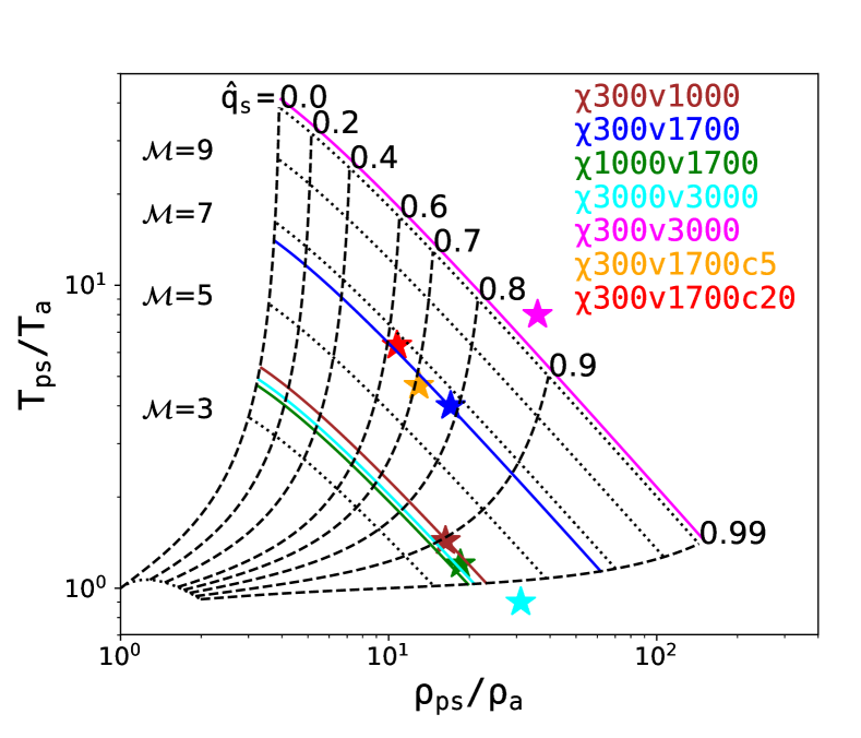
Figure 3: The ratio between the post-shock density and temperature, i.e., $\rho_{\mathrm{ps}}$ and $T_{\mathrm{ps}}$, and the pre-shock properties, i.e., $\rho_{\mathrm{a}}$ and $T_{\mathrm{a}}$, calculated for different sets of $(\hat{q}_{\mathrm{s}},\mathcal{M})$ pairs using the conductive jump conditions (Equation 12 and Equation 13). The $\mathcal{M}$ number is constant on each dotted line and $\hat{q}_{\mathrm{s}}$ is constant on each dashed line. The stars correspond to measurements from BS16 simulations, with the colours indicating particular numerical models as indicated in the figure. We also show solid lines that correspond to the $\mathcal{M}$ number of each simulation. Since the $\chi 300v1700$, $\chi 300v1700c5$ and $\chi 300v1700c20$ simulations use the same $\mathcal{M}=6.46$, we use a single blue line to indicate all three simulations.

However, the exact value of $\hat{q}_{\mathrm{s}}$ varies among simulations and is hard to determine from first principles. We measure these ratios from the BS16 simulations at $t_{\mathrm{90}}$, when the cloud reaches 90% of its original mass, and compare them to the analytic solutions in Figure 3. We find that the measured ratios lie close to the lines that are defined by their corresponding Mach number. However, $\hat{q}_{\mathrm{s}}$ varies among simulations that have a similar Mach number. In general, when thermal conduction is strong, as in the $\chi 3000v3000$ simulation where the ambient temperature is very high, $\hat{q}_{\mathrm{s}}$ is closer to unity, corresponding to a nearly isothermal shock. This is expected because, as the width of the bow shock develops over time, the temperature gradient after the shock gradually declines and the shock profile approaches an isothermal one. On the other hand, when thermal conduction decreases, as from the full Spitzer value $f_{\mathrm{s}}$ in $\chi 300v1700$ to $0.05f_{\mathrm{s}}$ in the $\chi 300v1700c20$ simulation, $\hat{q}_{\mathrm{s}}$ decreases.

In our model, we choose a constant $\hat{q}_{\mathrm{s}}=0.90$ whenever thermal conduction is non-negligible for simplicity.

In light of the conductive simulations from BS16, we further assume that the cloud will always have a cylindrical geometry after being compressed. We set the dimensions of the cloud as $(\pi R_{\mathrm{c}}^{2})\times L_{\mathrm{c}}$, where $R_{\mathrm{c}}$ is the cross section of the cloud perpendicular to the flow and $L_{\mathrm{c}}$ is the length of the cloud parallel to the flow. We set $L_{\mathrm{c}}=2R_{\mathrm{c}}$ immediately after the shock and can solve for $R_{\mathrm{c}}$ once the density of the compressed cloud $\rho_{4}$ is known. We also choose a coordinate system such that the $x-$axis is the central axis of the cylinder with the origin $x=0$ at the head of the cloud (Figure 4).

3.3 Expansion

After maximum compression from the cloud shock, the cloud expands rapidly in the downstream direction into a nearly vacuum cavity that is enclosed by the surface extended from the contact discontinuity. In simulations without thermal conduction (SB15), the expansion flow is often strongly perturbed by the ambient flow and quickly mixes into the ambient medium. In addition, a Rayleigh-Taylor instability at the front of the cloud often breaks up the cloud into smaller clumps, making the mixing process even more efficient. Therefore, in the non-thermal conduction regime, the clouds often do not have a well defined morphology.

In simulations with thermal conduction (BS16), the clouds often display a coherent, cylindrical morphology (e.g., see Figure 2). When thermal conduction is strong enough, it helps suppress hydrodynamic instabilities and confine the cloud with vapour pressure. Simulations also show a strong velocity gradient within the cloud throughout its expansion. In the velocity frame of the contact point at II, the expansion velocity increases linearly with the distance to the contact point and reaches a maximum at the tail of the cloud, where the cloud gas almost freely flows into the cavity with a speed comparable to the shock velocity $v_{s}$. However, when thermal conduction become less efficient, the cloud morphology becomes less stable and eventually the cloud breaks up faster.

Therefore, we will only approximate the cloud as a cylinder when thermal conduction is sufficiently strong (see Section 3.4 for more details on determining whether or not this is true). In our model with thermal conduction, it is important to know how the length of the cloud evolves with time, because the total evaporation rate from the cloud depends on the total surface area, i.e., $2\pi R_{\mathrm{c}}L_{\mathrm{c}}$, of the cloud at any time.

Immediately after the time of maximum compression, the velocity structure inside the simulated clouds resembles a similarity flow (Landau & Lifshitz, 1959), with the velocity at any point $x$, $v(x)$, increasing linearly with $x$. The flow in the cloud is a centred rarefaction wave until the wave propagates back to the location of the bow shock. The simulations show that the tail of the cloud often expands at a nearly constant velocity, $v_{\mathrm{exp}}$, so that the cloud length grows as $dL_{\mathrm{c}}/dt=v_{\mathrm{exp}}$. If the expansion is adiabatic, the cloud should expand at a terminal velocity $v_{\mathrm{max,ad}}=2c_{\mathrm{c}}/(\gamma-1)\sim 45$ km s^-1as expected from an adiabatic similarity flow. However, the $v_{\mathrm{exp}}$ measured from the simulations is often much larger than this value. Here, we assume the expansion is isothermal. For an isothermal similarity flow, the density $\rho_{\mathrm{c}}(x)$ and pressure $P_{\mathrm{c}}(x)$ at any position $x$ inside the expanding cloud are functions of the flow velocity $v(x)$ only:

$$\frac{\rho_{\mathrm{c}}(x)}{\rho_{\mathrm{c}}(0)}=\frac{P_{\mathrm{c}}(x)}{P_{\mathrm{c}}(0)}=\exp\left(-\frac{v(x)}{c_{\mathrm{c}}}\right),$$ (16)

where $\rho_{\mathrm{c}}(0)$ and $P_{\mathrm{c}}(0)$ are the density and pressure at the head of the cloud. Since the velocity $v(x)$ in an isothermally expanding cloud increases with $x$ and does not have an upper limit, we need to arbitrarily choose a maximum velocity as $v_{\mathrm{exp}}$, which corresponds to the velocity at the tail of the cloud. Equation 16 indicates that the cloud segment with a larger $v$ has a lower density and evaporates faster. Therefore, the further away from the head, the faster the cloud evaporates. In our model, we choose $v_{\mathrm{exp}}$ as the velocity at which the cloud still has not fully evaporated. At any time $t$, the fraction of the cloud where $v>v_{\mathrm{exp}}$, i.e., $\rho(v)<\rho(v_{\mathrm{exp}})$, has evaporated earlier. The $v_{\mathrm{exp}}$, therefore, decreases with time as

$$v_{\mathrm{exp}}\mathrm{(ev)}(t)=-c_{\mathrm{c}}\ln\left(4.5\times 10^{-15}\frac{T_{1}^{5/2}t}{\rho_{\mathrm{c}}(0)R_{\mathrm{c}}^{2}}\right),$$ (17)

where we use Equation 30 to find the evaporation rate per unit area $\dot{\hat{m}}_{\mathrm{A}}$ for classical conduction and use the temperature for the unperturbed ambient flow. The material that has velocities that exceed the expansion velocity are assumed to have evaporated.

On the other hand, we can choose $v_{\mathrm{exp}}$ as the velocity at which the cloud pressure equals the pressure of the unperturbed ambient, i.e., $P_{\mathrm{c}}(v_{\mathrm{exp}})=P_{1}$. Since the pressure at the head of the cloud, $P_{\mathrm{c}}(0)$ equals the ram pressure $P_{\mathrm{II}}$, the expansion velocity is:

$$v_{\mathrm{exp}}\mathrm{(P)}=-c_{\mathrm{c}}\ln\left(\frac{P_{1}}{P_{\mathrm{II}}}\right)$$ (18)

In practice, we choose the minimum value of these two velocities as the expansion velocity in our model:

$$v_{\mathrm{exp}}=\mathrm{min}\{v_{\mathrm{exp}}\mathrm{(ev)},v_{\mathrm{exp}}\mathrm{(P)}\}.$$ (19)

3.4 The Kelvin-Helmholtz Instability

The growth rate of perturbations at the interface of a shearing flow is characterised by the Kelvin-Helmholtz time-scale $\tau_{\mathrm{KH}}$. A classical analysis in the subsonic, incompressible limit shows that $\tau_{\mathrm{KH}}\propto\tau_{\mathrm{cc}}$ for linear growth (Chandrasekhar, 1961; Mandelker et al., 2016). In a supersonic flow, the KHI is damped, but the exact behaviour is poorly understood. Moreover, it is not straightforward to apply the classic $\tau_{\mathrm{KH}}$ to the cloud-crushing problem, where the geometry and long term evolution are distinct from those assumed in the classical analysis of the KHI. Radiative cooling also has a strong effect on the growth of the KHI (see Section 3.6 for details). Using their non-conductive simulations, SB15 obtain an empirical result for how fast the cloud loses mass in various situations. They find that the times at which the cloud has a certain fraction, e.g., 90%, 75%, 50%, 25%, of its original mass are proportional to $\tau_{\mathrm{cc}}\sqrt{1+\mathcal{M}_{\mathrm{h}}}$ (their equation 22). The additional $(1+\mathcal{M}_{\mathrm{h}})^{1/2}$ factor suggests that the clouds survive much longer in highly supersonic flows than that predicted from a classic analysis. Therefore, we adopt the following formula for clouds in regimes where thermal conduction is negligible:

$$\tau_{\mathrm{KH}}=f_{\mathrm{KH}}\sqrt{1+\mathcal{M}_{1}},$$ (20)

where $f_{\mathrm{KH}}$ is a free parameter of order unity that controls how fast clouds lose mass via KHI, and $\mathcal{M}_{1}=v_{\mathrm{rel}}/c_{1}$ is the Mach number of the flow relative to the cloud. We calculate the mass loss rate of the cloud as:

$$\dot{M}_{\mathrm{c;KH}}=\frac{M_{\mathrm{c}}}{\tau_{\mathrm{KH}}}.$$ (21)

Whether or not KHI can grow depends also on the strength of thermal conduction. In the extreme case where evaporation dominates over the ambient flow, it simply eliminates any velocity shear. With less strong thermal conduction, linear perturbations on the cloud surface can still be stabilised if the kinetic energy diffuses quickly enough before it can generate a significant amount of local vorticity.

A full treatment of this problem requires solving the linearly perturbed equations that include a conductive flux term in the energy equation, which is very challenging even in ideal situations. Here we derive an approximate criterion based on whether or not the diffusion time-scale owing to thermal conduction, $\tau_{\mathrm{diff}}$, is shorter than the mixing time-scale, $\tau_{\mathrm{mix}}$, owing to KHI.

Consider a hot phase with density $\rho_{\mathrm{h}}$ and temperature $T_{\mathrm{h}}$ flowing at a relative velocity of $v_{\mathrm{rel}}$ to a cold phase with density $\rho_{\mathrm{c}}=\chi\rho_{\mathrm{h}}$ and temperature $T_{\mathrm{c}}$. A perturbation on the scale of $\lambda$ in the cloud will mix into the ambient flow over a finite width $\lambda$ within $\tau_{\mathrm{mix}}$ without thermal conduction. We can obtain the mixing time-scale using the dispersion relation for the growth of linear perturbations (Mandelker et al., 2016):

$$\tau_{\mathrm{mix}}\sim\chi^{1/2}\lambda/v_{\mathrm{rel}}.$$ (22)

To calculate the diffusion time-scale, we consider how long it takes the conductive heat flux to fully mix the kinetic and thermal energy between a density perturbation with its surroundings on any scale $\lambda$:

$$\tau_{\mathrm{diff}}=\frac{1}{1+\chi}\frac{\rho_{\mathrm{c}}\lambda[v_{\mathrm{rel}}^{2}/2+3c_{\mathrm{h}}^{2}/2]}{q},$$ (23)

where $c_{\mathrm{h}}$ is the sound speed of the hot gas, the factor $1/(1+\chi)$ is the volume filling factor for the cold phase, and $q$ is the conductive heat flux. Here we assume classical conduction and approximate it as $q=f_{\mathrm{s}}\kappa_{\mathrm{h}}(T_{\mathrm{h}}/\lambda)$. There exists a critical scale $\lambda_{\mathrm{KH}}$ where $\tau_{\mathrm{diff}}=\tau_{\mathrm{mix}}$. Perturbations are able to grow only on scales smaller than $\lambda_{\mathrm{KH}}$:

$$\lambda_{\mathrm{KH}}=\frac{1+\chi}{\chi^{1/2}}\frac{1}{\mathcal{M}_{\mathrm{h}}(\mathcal{M}_{\mathrm{h}}^{2}+3)}\frac{f_{\mathrm{s}}\kappa_{\mathrm{h}}}{n_{\mathrm{h}}T_{\mathrm{h}}^{1/2}}\left(\frac{4\mu m_{\mathrm{H}}}{\gamma^{3}k_{\mathrm{B}}^{3}}\right)^{1/2},$$ (24)

where $n_{\mathrm{h}}$ and $\mathcal{M}_{\mathrm{h}}$ are the hydrogen number density and the Mach number of the hot phase, respectively. In the cloud-crushing problem, the KHI is able to grow only when $R_{\mathrm{c}}>\lambda_{\mathrm{KH}}$. Using $\chi\gg 1$, and $\mathcal{M}_{\mathrm{h}}\sim 1$ for the post-shock gas, we can write $\lambda_{\mathrm{KH}}$ numerically as:

$$\lambda_{\mathrm{KH}}=5.7\ [\mathrm{kpc}]\ f_{\mathrm{s}}\left(\frac{\chi}{10^{2}}\right)^{1/2}\left(\frac{T_{\mathrm{h}}}{10^{7}\,\mathrm{K}}\right)^{2}\left(\frac{n_{\mathrm{h}}}{10^{-2}\ \mathrm{cm^{-3}}}\right)^{-1}.$$ (25)

Mandelker et al. (2016) find a similar dependence of $\lambda_{\mathrm{KH}}$ on fluid properties, i.e., $\lambda_{\mathrm{KH}}\propto T_{\mathrm{h}}^{2}n_{\mathrm{h}}^{-1}\mathcal{M}_{\mathrm{h}}^{-1}$. For most of the simulations from BS16 with full Spitzer rate conduction, i.e., $f_{\mathrm{s}}=1$, the critical length $\lambda_{\mathrm{KH}}$ is much larger than the cloud radius $R_{\mathrm{c}}$, so that the Kelvin-Helmholtz instabilities are always suppressed.

However, when one reduces $f_{\mathrm{s}}$, KHI will eventually be able to grow. In the three $\chi 300v1700$ simulations, using properties of the ambient flow of $n_{\mathrm{II}}\sim 0.1\ \mathrm{\mathrm{cm}^{-3}}$, $T_{\mathrm{II}}\sim 7\times 10^{6}\,\mathrm{K}$, and $\chi\sim 10^{3}$, we find that the critical scales for the $\chi 300v1700$, $\chi 300v1700c5$, and the $\chi 300v1700c20$ simulations are 890 pc, 178 pc, and 45 pc, respectively. Only in the $\chi 300v1700c20$ simulation is the critical scale comparable to the cloud radius $R_{\mathrm{c}}\sim 20\,\mathrm{pc}$, and this is the only simulation that indeed shows some growth of the KHI at later times that ultimately breaks up the cloud. In Section 5 we will show that KHI indeed causes the cloud to lose mass in addition to evaporation.

3.5 The Conduction Zone

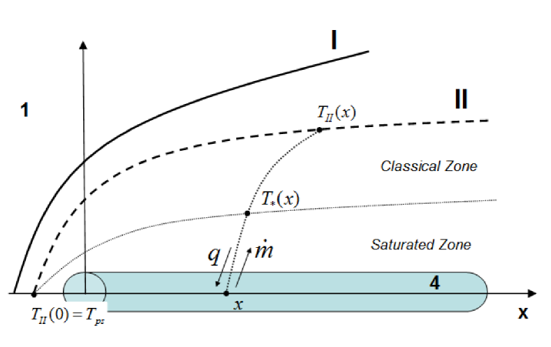
Figure 4: An illustration of our method of calculating the conductive evaporation rate from the cloud at any given time. We assume cylindrical symmetry. Roman and Arabic numerals have the same meanings as in Figure 1. We assume that thermal conduction between the cloud and the ambient flow causes heat flux and evaporation within a conduction zone bounded by the surface of the cloud and an arbitrarily chosen streamline (noted as Roman numeral II) in the ambient flow. Depending on the strength of the conduction, the region may be divided into a classic zone and a saturated zone separated by a transition surface, where the quantities are subscribed with a star symbol (*).

When thermal conduction is strong, cold gas evaporates from the cloud surface and mixes into the ambient flow moving downstream. To solve for the mass loss rate from the cloud, we assume that the flow is axisymmetric and that there exists a continuous conduction zone (see Figure 4) extending from the cloud surface III to an arbitrary surface II in the ambient flow. Inside the conduction zone, the gas that evaporated from any coordinate $x$ in the cloud is heated from the cloud temperature $T_{\mathrm{c}}$ to a corresponding ambient temperature at the surface II, i.e., $T_{\mathrm{II}}(x)$. The temperature varies along the streamlines, dropping from the maximum value at the shock front $T_{ps}$ (or $T_{2}$ as in Figure 1), to the unperturbed ambient temperature $T_{1}$ far behind the shock. We now focus on streamlines (dotted lines) along which the evaporated material flows. Each of these paths relates fluid properties at one point on the cloud to those at another point on the surface II. We approximate these streamlines of evaporated material as radial to the clouds so that we can analytically integrate over the radial coordinate $r$ from the cloud surface $r=R_{\mathrm{c}}$ to the ambient $r=r_{\mathrm{II}}$. The problem is to find an approximate expression for $T_{\mathrm{II}}(x)$, parameterized by the cloud coordinate $x$, and to find the mass loss rate per unit area $dA=2\pi R_{\mathrm{c}}dx$ at any $x$ of the cloud, defined as:

$$\dot{\hat{m}}_{\mathrm{A}}=2\pi r\rho v=\mathit{const.}$$ (26)

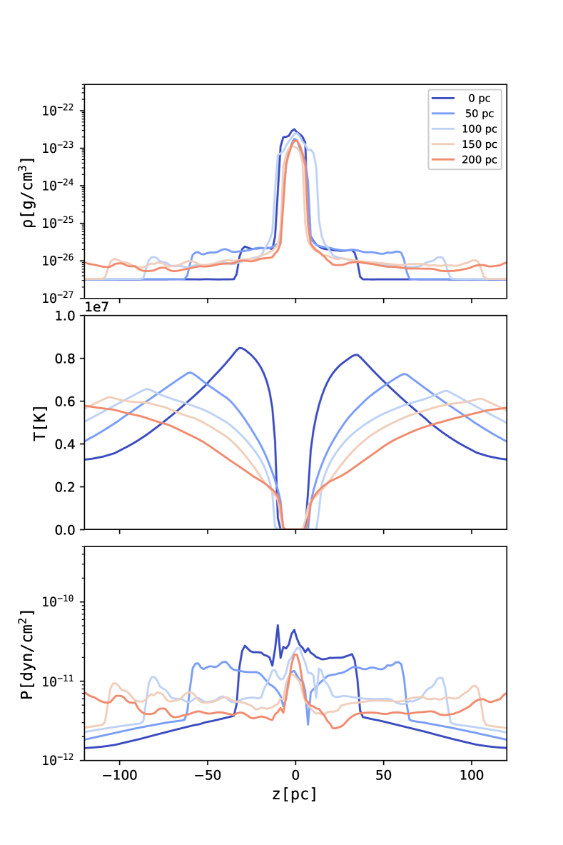
Figure 5: The radial profiles of density (upper panel), temperature (middle panel) and pressure (lower panel) at different cross sections of a simulated cloud. The data is from the $\chi 300v1700$ simulation at $t_{\mathrm{75}}$. The legend shows how far the cross section is from the head. Note that the temperature axis in the middle panel is shown in linear scale, so it’s clear that the temperature gradient sharpens towards the cloud, making thermal conduction more likely to saturate.

We show a typical conduction zone from the simulations in Figure 5. The profiles show three distinct regions, separated by two sharp density discontinuities. From inside out, the three regions correspond to the cloud, the post-shock ambient flow (conduction zone), and the flow outside the bow shock. The conduction zone broadens with the distance from the head (from blue to red), consistent with the morphology illustrated in Figure 1. The lateral dimension of the cloud, i.e. $R_{\mathrm{c}}$, varies little along the cloud.

In the conduction zone, the temperature gradient sharpens towards the cloud surface, where the conductive flux will likely start to saturate. When thermal conduction is strong enough, there exists a critical point where the heat flux starts to saturate so that it divides the conduction zone into a classic zone and a saturated zone, which will be treated separately below. The flow properties at the critical point are noted as $\rho_{*}$, $T_{*}$, etc.

In both regions, the flow along any path is governed by the time-independent Euler equations in cylindrical coordinates:

$$\rho\frac{dv}{dr}+v\frac{du}{dr}+\frac{\rho v}{r}=0,$$ (27)

$$\rho v\frac{dv}{dr}=-\frac{dp}{dr},$$ (28)

and

$$\frac{3}{2}\gamma\dot{\hat{m}}_{\mathrm{A}}(1+\frac{1}{5}\mathcal{M}^{2})c^{2}=2\pi rq.$$ (29)

All flow quantities in the above equations are functions of $r$. The heat flux $q$ is determined by either Equation 1 or Equation 3 in the classical and the saturated zone, respectively. In the classical zone, $\mathcal{M}^{2}/5\ll 1$ so that $\dot{\hat{m}}_{\mathrm{A}}\propto rq_{\mathrm{class}}/T$. Since $\dot{\hat{m}}_{\mathrm{A}}$ is constant along the streamline, $q_{\mathrm{class}}$ is proportional to $T/r$, which decreases with $r$. There might exist a critical point $r=r_{*}$, where $q_{\mathrm{sat}}=q_{*}=q_{\mathrm{class}}$. At $r<r_{*}$, $\sigma_{0}>1$, this corresponds to saturated conduction, while at $r>r_{*}$, $\sigma_{0}<1$, this corresponds to classical conduction. We further define $\sigma_{*}$ and $\sigma_{\mathrm{c}}$ as the value of $\sigma_{0}$ at $r=r_{*}$ and $r=R_{\mathrm{c}}$, respectively. By definition, $\sigma_{*}=1$. Therefore, the critical point exists if and only if $\sigma_{\mathrm{c}}>1$.

In the classical zone, we could obtain $\dot{\hat{m}}_{\mathrm{A}}$ by integrating the energy equation (Equation 29) from $r=r_{*}$ to $r=r_{\mathrm{II}}$ using Equation 1 with the approximation that $1+\mathcal{M}^{2}/5\sim 1$:

$$\dot{\hat{m}}_{\mathrm{A}}\mathrm{(class)}=6.1\times 10^{-7}f_{\mathrm{r}}^{-1}\left(\frac{8\pi\mu m_{\mathrm{H}}}{15\gamma k_{\mathrm{B}}}\right)(T_{\mathrm{II}}^{5/2}-T_{*}^{5/2}),$$ (30)

where $f_{\mathrm{r}}\equiv\ln(r_{\mathrm{II}}/R_{\mathrm{c}})$ is of order unity. We will use $f_{\mathrm{r}}=1$ in this paper.

In the saturated zone, integrating the energy equation Equation 29 shows that the Mach number has a constant value $\mathcal{M}_{\mathrm{sat}}$ that is determined by

$$\mathcal{M}_{\mathrm{sat}}(1+\frac{1}{5}\mathcal{M}_{\mathrm{sat}}^{2})=2f_{\mathrm{s}},$$ (31)

where $\mathcal{M}_{\mathrm{sat}}\sim 1.4$ throughout the saturated zone for thermal conduction at the full Spitzer rate, i.e., $f_{\mathrm{s}}=1$, and becomes smaller with a reduced $f_{\mathrm{s}}$.

With a constant $\mathcal{M}_{\mathrm{sat}}$, we can solve for the temperature profile in the saturated zone by integrating the continuity equation (Equation 27) and the equation of motion (Equation 28) in cylindrical coordinates:

$$\left(\frac{T}{T_{\mathrm{c}}}\right)=\left(\frac{r}{R_{\mathrm{c}}}\right)^{2/(1+\mathcal{M}_{\mathrm{sat}}^{2})}.$$ (32)

To provide a boundary condition at $r_{*}$ for the saturated zone, we further assume that the pressure gradient in the classical zone is negligible as indicated by the simulation (Figure 5), so that

$$n_{*}T_{*}=n_{\mathrm{II}}T_{\mathrm{II}}.$$ (33)

We can solve for the mass loss rate in the saturated zone with Equation 29, Equation 31 and Equation 33:

$$\begin{split}\dot{\hat{m}}_{\mathrm{A}}\mathrm{(sat)}=&\,1.715\times 10^{-11}\left(\frac{4\pi}{3+\mathcal{M}_{\mathrm{sat}}^{2}}\right)\left(\frac{\mu m_{\mathrm{H}}}{\gamma k_{\mathrm{B}}}\right)\times\\ &\,T_{*}^{-1/2}\left(\frac{n_{\mathrm{II}}T_{\mathrm{II}}}{R_{\mathrm{c}}}\right)\left(\frac{T_{\mathrm{c}}}{T_{*}}\right)^{(1+\mathcal{M}_{\mathrm{sat}}^{2})/2}.\end{split}$$ (34)

We can find the temperature at the critical point $T_{*}$ by iteratively solving the equation $\sigma_{*}=1$, where the saturation parameter, $\sigma_{*}$, is by definition the ratio $q_{\mathrm{class}}/q_{\mathrm{sat}}$ at $r_{*}$:

$$\begin{split}\sigma_{*}=&\,3.6\times 10^{4}f_{\mathrm{r}}^{-1}\left(\frac{6+2\mathcal{M}_{\mathrm{sat}}^{2}}{15}\right)\times\\ &\,\left[\frac{(T_{\mathrm{II}}^{5/2}-T_{*}^{5/2})T_{*}^{1/2}}{n_{\mathrm{II}}T_{\mathrm{II}}R_{\mathrm{c}}}\right]\left(\frac{T_{\mathrm{c}}}{T_{*}}\right)^{(1+\mathcal{M}_{\mathrm{sat}}^{2})/2}.\end{split}$$ (35)

A solution for $T_{*}$ is physical only if $T_{*}\geq T_{c}$. It is clear from Equation 35 that $\sigma_{*}$ increases with $r$ so that $\sigma_{*}\geq\sigma_{\mathrm{c}}$. Therefore, the criterion that a saturated zone exists is $\sigma_{\mathrm{c}}\geq 1$. Using a fiducial set of parameters, $f_{\mathrm{r}}=f_{\mathrm{s}}=1$, this criterion becomes:

$$\sigma_{\mathrm{c}}=2.4\times 10^{4}\left[\frac{(T_{\mathrm{II}}^{5/2}-T_{\mathrm{c}}^{5/2})T_{\mathrm{c}}^{1/2}}{n_{\mathrm{II}}T_{\mathrm{II}}R_{\mathrm{c}}}\right]\geq 1.$$ (36)

We then obtain the total evaporative mass loss rate of the cloud through integration over $x$:

$$\begin{split}\dot{M}_{\mathrm{c,ev}}&=\int_{0}^{L_{\mathrm{c}}}2\pi R_{\mathrm{c}}\dot{\hat{m}}_{\mathrm{A}}(x)dx\\ &=\frac{1}{f_{\mathrm{m}}}2\pi R_{\mathrm{c}}L_{\mathrm{c}}\dot{\hat{m}}_{\mathrm{A}}(0)\end{split},$$ (37)

where we introduce $f_{\mathrm{m}}$ as a parameter that simplifies the integral. We approximate the integral by using a constant value for the mass loss rate along the cloud $\dot{\hat{m}}_{\mathrm{A}}(0)$ and apply a correction factor $f_{\mathrm{m}}$ to account for actual variations along the cloud. Since the temperature gradient is strongest near the head ($x=0$), the conduction rate and the mass loss rate are also highest there. Therefore, $f_{\mathrm{m}}>1$. Appendix C estimates that $f_{\mathrm{m}}=3.5$ under the simplified assumption that thermal conduction is nowhere saturated. We adopt this value $f_{\mathrm{m}}=3.5$ throughout this paper.

3.6 The Effects of Radiative Cooling

For simulations that include thermal conduction, radiative cooling dominates over conductive heating over distances larger than the Field length, $L_{\mathrm{F}}$ (Field, 1965):

$$L_{\mathrm{F}}=\left(\frac{\kappa_{\mathrm{h}}T_{\mathrm{h}}}{n_{\mathrm{c}}^{2}\Lambda_{\mathrm{c}}}\right)^{1/2},$$ (38)

where $\kappa_{\mathrm{h}}$ and $T_{\mathrm{h}}$ are the conductive coefficient and the temperature of the hot ambient medium, respectively, and $n_{\mathrm{c}}$ and $\Lambda_{\mathrm{c}}$ are the density and the cooling function of the cloud, respectively. Both analytic (Begelman & McKee, 1990) and numerical (e.g. Armillotta et al., 2016) works suggest that clouds much larger than the Field length ($R_{\mathrm{c}}\gg L_{\mathrm{F}}$) will condense as radiative cooling dominates and that clouds much smaller than the Field length ($R_{\mathrm{c}}\ll L_{\mathrm{F}}$) will evaporate as thermal conduction dominates. Both processes need to be considered when the two scales are comparable to each other. It is unclear whether or not clouds will evaporate in this physical regime, especially if the cloud is moving relative to the ambient medium. Previous works that compare these two scale lengths often assume that the cloud is static. In this case, a temperature gradient of scale $l_{\mathrm{T}}$ is allowed to develop at the initially discontinuous interface. Since the energy exchange rate owing to thermal conduction scales as $T/l_{\mathrm{T}}^{2}$, conduction becomes less efficient as the gradient grows until $l_{\mathrm{T}}\sim L_{\mathrm{F}}$, where it is balanced by cooling. When the cloud is moving, however, the ambient flow will prevent such a gradient from growing thus keeping thermal conduction efficient. Therefore, the cloud likely still evaporates when $R_{\mathrm{c}}\sim L_{\mathrm{F}}$.

In most of the simulations from BS16, the cloud radius after the initial shock is smaller than $L_{\mathrm{F}}$, except for the $\chi 300v1000$ simulation. Therefore, we assume that conduction-driven evaporation dominates over cooling-driven condensation in our model. However, one should be cautious about the effect of radiative cooling when applying our model to cosmological simulations.

Radiative cooling can also strongly affect the growth of the KHI. The evolution of KHI in shearing flows with cooling have been studied using numerical simulations that assume different geometries, e.g., 2D, 3D, slab, cylindrical, etc. Strong radiative cooling prevents the mixing layer at the interface from growing and penetrating into the cloud (Vietri et al., 1997) and suppresses the linear growth of the KHI. However, whether or not cooling can enhance (Stone et al., 1997; Xu et al., 2000) or suppress (Rossi et al., 1997; Vietri et al., 1997; Micono et al., 2000) the long term non-linear evolution of KHI is likely sensitive to the details of the numerics, flow parameters, and cooling functions. Many of these earlier studies focus on the context of the interstellar medium (ISM), e.g., between proto-stellar jets and their surrounding medium of $\sim 10^{4}\,\mathrm{K}$, where the physical conditions are very different from the hot halo environment.

The effect of radiative cooling has also been directly studied in cloud-crushing simulations. In general, efficient cooling helps compress the cloud to higher densities, making it more resistant to hydrodynamic instabilities (Klein et al., 1994; Armillotta et al., 2016; Li et al., 2019), but the effects are hard to quantify. This again motivates us to use a parameterized formula (Equation 20) to describe the KHI-driven mass loss rate of the cloud. Recent simulations also suggest that radiative cooling could drive thermal instabilities and cause the cloud to fragment to characteristic scales (McCourt et al., 2018; Sparre et al., 2019), but the stripped gas from the cloud could also condense and reform cloudlets in the downstream flow under certain conditions where cooling is efficient (Gronke & Oh, 2018; Li et al., 2019). However, we do not model these processes in this paper.

4 Modelling the Evolution of the Cloud

In this section, we give a step-by-step recipe for evolving the cloud analytically (Section 4.1). Remember that we assume that each wind particle is a collection of clouds, each with a mass $M_{\mathrm{c}}$, whose number depends on the wind particle mass and $M_{\mathrm{c}}$. We also summarise our main assumptions and approximations and discuss the robustness of these assumptions in Section 4.2.

4.1 The Analytic Model

When a cloud with initial mass $M_{\mathrm{c}}$ enters into the ambient medium at supersonic speed as shown in Figure 1, we first calculate the properties related to the bow shock and the cloud shock.

Cloud shock. The jump conditions (Equations 12 and 13) determine the post-shock pressure

$$\frac{P_{\mathrm{II}}}{P_{1}}\sim\left[\frac{2\gamma}{\gamma+1}\mathcal{M}_{1}^{2}-\frac{\gamma-1}{\gamma+1}\right]\eta_{\mathrm{s}}\tau_{\mathrm{s}},$$ (39)

where $\eta_{\mathrm{s}}$ and $\tau_{\mathrm{s}}$ are the corrections to the jump conditions for density and temperature owing to thermal conduction (Equations 53 and 54) and should both be 1 when thermal conduction is inefficient. The pressure across the contact discontinuity II is the same, i.e., $P_{\mathrm{II}}=P_{4}$. We can solve for the post-shock cloud density $\rho_{4}$ and cloud radius $R_{\mathrm{c}}$ under the assumption of an isothermal cloud shock ($T_{\mathrm{eq}}=10^{4}K$):

$$\frac{\rho_{4}k_{\mathrm{B}}T_{\mathrm{eq}}}{\mu m_{H}}=P_{\mathrm{II}}$$ (40)

and

$$2\rho_{4}R_{\mathrm{c}}(\pi R_{\mathrm{c}}^{2})=M_{\mathrm{c}}.$$ (41)

Here, we assume that the cloud shock is nearly isotropic so that at maximum compression the two dimensions of the cylindrical cloud are comparable to one another, i.e., $L_{\mathrm{c}}=2R_{\mathrm{c}}$. The cloud shock in general takes 1 to 2 cloud crushing time to complete.

Confined expansion. This only applies when thermal conduction is sufficiently strong to maintain the coherence of the cloud. When thermal conduction is weak, we proceed to calculate the mass loss rate and the deceleration of the cloud. The over-pressured cloud expands in the downstream direction at a speed $v_{\mathrm{exp}}$, which we determine from Equation 19. The length of the cloud evolves with time as $L_{\mathrm{c}}(t)=L_{\mathrm{c}}(t=0)+v_{\mathrm{exp}}t$. We also allow the lateral dimension of the cloud $R_{\mathrm{c}}$ to change with $M_{\mathrm{c}}$:

$$R_{\mathrm{c}}=\left(\frac{M_{\mathrm{c}}}{\pi\mu m_{H}n_{\mathrm{c}}L_{\mathrm{c}}}\right)^{1/2},$$ (42)

where $N_{\mathrm{c}}$ is the total column number density along the flow direction, which is kept constant over time, i.e., $N_{\mathrm{c}}=n_{4}L_{\mathrm{c}}(t=0)$. The $R_{\mathrm{c}}$ calculated from Equation 42 is consistent with the radius of the clouds in the numerical simulations.

Mass loss. The cloud loses mass owing to both the KHI (Equation 21) and evaporation (Equation 37). To calculate the evaporative mass loss rate per unit area at the head, i.e., $\dot{\hat{m}}_{\mathrm{A}}(0)$, we first determine whether or not a saturated zone exists using the criterion from Equation 36. If it does exist, we calculate $T_{*}$ by iteratively solving the equation $\sigma_{*}=1$ using Equation 35 and then find the mass loss rate using Equation 34. If it does not exist, we find the mass loss rate using Equation 30 with $T_{*}$ set to $T_{\mathrm{c}}$ in the equation.

We calculate the total mass loss rate as

$$\dot{M}_{\mathrm{c}}=\dot{M}_{\mathrm{c,KH}}\exp(-R_{\mathrm{c}}/\lambda_{\mathrm{KH}})+\dot{M}_{\mathrm{c,ev}},$$ (43)

where $\dot{M}_{\mathrm{c,KH}}$ and $\dot{M}_{\mathrm{c,ev}}$ are mass loss rate from the KHI and evaporation alone, respectively. Since strong thermal conduction suppresses the KHI, we suppress $\dot{M}_{\mathrm{c,KH}}$ by a factor of $\exp(-R_{\mathrm{c}}/\lambda_{\mathrm{KH}})$, where $\lambda_{\mathrm{KH}}$ is determined by Equation 24. Therefore, the contribution from KHI decreases sharply when $R_{\mathrm{c}}\gg\lambda_{\mathrm{KH}}$ and only becomes important when $R_{\mathrm{c}}\ll\lambda_{\mathrm{KH}}$.

Deceleration. The cloud slows down as a result of the ram pressure $P_{\mathrm{II}}$. At anytime $t$, the cloud decelerates as:

$$\dot{v}_{\mathrm{rel}}=\frac{P_{\mathrm{II}}\pi R_{\mathrm{c}}^{2}(t)}{M_{\mathrm{c}}(t)}.$$ (44)

Following the above procedures we can solve for the cloud properties $\rho_{4}(t,x)$, $M_{\mathrm{c}}(t)$, $v_{\mathrm{rel}}(t)$, $R_{\mathrm{c}}(t)$, $L_{\mathrm{c}}(t)$ at any given time by numerical integration.

4.2 Simplifications

Here we discuss the key simplifications in our model in the limit of strong thermal conduction. These simplifications are largely corroborated by the numerical simulations of BS16, and are essential for the model to reproduce their results even qualitatively.

Isothermal cloud. In BS16, the cloud is initially in thermal equilibrium with a temperature $T_{\mathrm{eq}}\sim 10^{4}\,\mathrm{K}$. At this temperature, radiative cooling is so efficient that during the evolution, the cloud remains nearly isothermal. Therefore, we assume that the cloud temperature $T_{\mathrm{eq}}$ is invariant in our model. This also assumes that the cloud shock is isothermal, which allows the cloud to be shocked to high density. However, this assumption breaks down if the Field length is comparable to the cloud size.

In some simulations, the tail of the cloud expands so fast that during the first few $\tau_{\mathrm{cc}}$ after the cloud shock parts of the cloud can be much colder than $T_{\mathrm{eq}}$. However, the adiabatically cooled tail soon heats up and hence this deviation does not significantly affect the behaviour of the bulk of the cloud since most of the cloud mass concentrates in the dense, slowly-expanding front of the cloud.

Constant $\hat{q}_{\mathrm{s}}$ parameter. We use a constant value (0.9) for the $\hat{q}_{\mathrm{s}}$ parameter, i.e., ratio between the kinetic energy flux and the conductive heat flux across the bow shock, whenever thermal conduction dominates. In general, $\hat{q}_{\mathrm{s}}$ decreases from our chosen value when thermal conduction is sufficiently weak. However, this transition from high $\hat{q}_{\mathrm{s}}$ values (e.g., 0.9), to $\hat{q}_{\mathrm{s}}\sim 0$ (non-conductive) is very sharp, because the strength of thermal conduction is very sensitive to temperature. Therefore, deviations from this simplification will only affect a small range of temperatures. Moreover, since thermal conduction is weak in these situations, the evolution of the cloud is much less sensitive to the value of $\hat{q}_{\mathrm{s}}$ than where constant $\hat{q}_{\mathrm{s}}$ is a good approximation.

Cylindrical geometry. In our model, when thermal conduction is efficient, we let the cloud expand only in the downstream direction so that over time the cloud becomes elongated with $L_{\mathrm{c}}\gg R_{\mathrm{c}}$ as seen in the simulations of BS16. The elongation helps keep the cross section of the cloud small, which keeps the cloud from slowing down too fast. It also results in a larger surface area between the cloud and the ambient flow, which makes the cloud evaporate much faster.

Similarity flow in the cloud. We approximate the flow inside the cloud as an isothermal similarity flow, which parametrises the density and the pressure anywhere inside the cloud with the flow velocity only (see section 3.3 for details). This implies that cloud density declines logarithmically from the front to the end of the cloud, which is approximately true in BS16. However, some of their simulations show that some density sub-structures emerge in the cloud later in the evolution, and that the cloud eventually breaks up into smaller aligned clumps.

KHI suppression. The Kelvin-Helmholtz instability, as well as other hydrodynamic instabilities that lead to the fragmentation of the cloud, are suppressed by efficient thermal conduction. This is clearly demonstrated in BS16, where clouds, as long as they do not evaporate too soon, are able to maintain a coherent structure for much longer than those in the same physical conditions but without conduction (SB15).

Small vapour pressure. We approximate that the vapour pressure is negligible compared to the post-shock thermal pressure so that the internal pressure of the cloud is balanced by thermal pressure only. Simulations indicate that at least in the front shock, the thermal pressure calculated from the conductive jump conditions are comparable to the cloud pressure except for the $\mathcal{M}=1$ cases. Inside the oblique shock (region 5), whether or not vapour pressure is important is uncertain as it is hard to compute.

Post-shock ambient flow. The flow between boundary I and boundary III is a mixture of the shocked ambient gas and the evaporated material from the cloud. The flow properties here are crucial to calculating the evaporation rate from the cloud, because the conductive flux is very sensitive to the temperature gradient. To solve for the time-dependent Eulerian equations with boundary conditions at both the oblique shock front (boundary I) and the cloud surface (boundary III) is very complicated. Therefore, we simplify the problem with several approximations that are detailed in Section 3.5. Namely, we assume that the flow is continuous everywhere and can be described using Bernoulli’s equations. However, when thermal conduction is too strong, e.g., in the $\chi 3000v3000$ simulation where $T_{1}=3\times 10^{7}\,\mathrm{K}$, the evaporation becomes supersonic and creates shocks in the ambient flow, violating the continuity assumption. We note that the condition for supersonic evaporation is likely similar to that for vapour pressure to be dominant. In both cases, the thermal conduction must be very saturated ($\sigma_{0}\gg 1$).

No self-gravity. The Jeans mass of the shock compressed cloud, assuming a number density of $10\,\mathrm{cm}^{-3}$ and a temperature of $10^{4}\,\mathrm{K}$, is $8\times 10^{7}M_{\odot}$, much larger than $M_{\mathrm{c}}$. Therefore self-gravity is almost never important in this study, unless the cloud is allowed to cool to much below the equilibrium temperature.

5 TESTS

In Figures 6, 7 and 9, we compare the analytic results to simulations. For comparison, we also calculate the cloud evolution using a simple spherical model as described below.

5.1 A Spherical Model

Semi-analytic models for clouds entrained in hot winds or clouds that travel in the haloes often assume the clouds are spheres with a uniform density (Zhang et al., 2017; Lan & Mo, 2019). Here, to compare with the cylindrical model, we examine whether or not a simpler spherical cloud model can reproduce the simulation results.

We define the properties of the cloud and the ambient medium using the same diagram as in Figure 1. Many quantities are determined the same way as in the cylindrical model, except that now $\rho_{4}$ is constant over the cloud and $R_{\mathrm{c}}$ is the radius of the sphere changing with time.

The properties of the bow shock and the cloud shock are determined by Equations 39 and 40. After the cloud shock, the cloud radius is determined by

$$R_{\mathrm{c}}(t)=\left(\frac{3M_{\mathrm{c}}(t)}{4\pi\rho_{4}(t)}\right)^{1/3}.$$ (45)

At each time-step after the cloud shock, we assume that the cloud is always in pressure equilibrium with the post-shock ambient gas, so that $P_{4}=P_{\mathrm{II}}$. The cloud density at any time can then be derived from the pressure using Equation 40.

To calculate the evaporation rate at any given time, we use the CM77 formulation (Equations 6 and 7), which is derived for a spherical cloud in a static medium. Since here we only compare the model to conductive simulations from BS16, we assume that KHI is always suppressed.

The deceleration of the cloud is governed by Equation 44.

5.2 Mass Loss

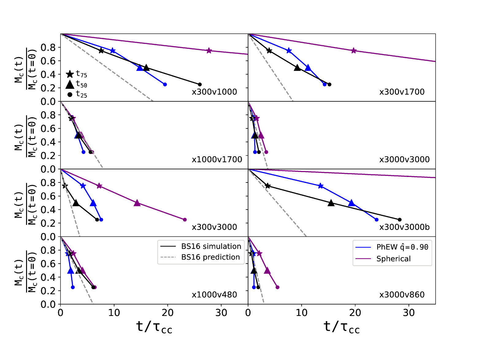
Figure 6: Each panel shows the fraction of dense gas that remains in the cloud as a function of time in units of the cloud crushing time $\tau_{\mathrm{cc}}$. Stars, triangles and circles indicate values at $t_{\mathrm{75}}$, $t_{\mathrm{50}}$, $t_{\mathrm{25}}$, i.e., when the cloud has reached 75%, 50% and 25% of its original mass, respectively. The black symbols are results from the cloud-crushing simulations of BS16. They provide an analytic formula (their equation 17) for the mass loss rate. We show this prediction as the grey dashed lines. The blue symbols are predictions from our fiducial model assuming a constant $\hat{q}_{\mathrm{s}}=0.90$. The purple symbols are predictions from the simple spherical model (Section 5.1). The names of the simulations are indicated in the bottom right corner of each panel.

In Figure 6, we compare our model predictions of the mass evolution of the cloud to results from the simulations of BS16, in which the cloud mass at any given time is defined as the total mass above a density threshold $\rho_{th}=\rho_{1}/3$, where $\rho_{1}$ is the original density of the cloud. This threshold is sufficient to capture most of the cold gas remaining in the cloud because the cloud shock has compressed it to a much higher density than $\rho_{1}$. Mass loss is dominated by conductive evaporation in these simulations. In our fiducial analytic model, the cloud mass $M_{\mathrm{c}}(t)$ evolves with time according to Equation 37.

The spherical model presented above significantly over-estimates the lifetime of the cloud in most cases. The larger surface areas of the elongated clouds in our fiducial model play a critical role in quickly evaporating the cloud. The spherical model agrees with the simulations only in the two extreme cases, $\chi 1000v1700$ and $\chi 3000v3000$. In both of these cases, the shocked ambient gas is so hot ($T_{5}>10^{7}\,\mathrm{K}$) that some of our simplifications for the fiducial model might break down. First, thermal conduction is so strong that the evaporation time-scale is shorter than the dynamic time-scale for expansion. Second, the vapour pressure dominates over thermal pressure in driving the cloud shock, which in these cases compresses the cloud to higher densities nearly isotropically. Both of these effects tend to make the cloud more spherical in morphology. Therefore, the CM77 solution for spherical clouds describes the evolution of the cloud better than in the other simulations.

Our fiducial model qualitatively agrees with the simulations in all the cases shown here. The model over-estimates the mass loss rate for the $\chi 1000v1700$ and $\chi 3000v3000$ cases for the reasons discussed in the last paragraph. In the other simulations, the cloud loses mass more rapidly during the first few $\tau_{\mathrm{cc}}$, reaching $t_{\mathrm{75}}$ earlier than in our model, but this is because we only allow mass loss from the cloud after the cloud shock. During the expansion phase, our model slightly over-estimates the mass loss rate, e.g., in the $\chi 300v3000b$ case. This is likely because of differences in the internal structures of the cloud at later times. In the simulations, density perturbations develop in the cloud with time and eventually break the cloud into smaller, denser clumps, but in our model we assume that the cloud always maintains a coherent cylindrical geometry with a logarithmic density structure, resulting in a larger total surface area and stronger evaporation.

In Figure 6, we also compare our model predictions to the analytic results derived in BS16. They assume a constant mass loss rate from the cloud (their equation 17) until it completely mixes with the surroundings over an evaporation time-scale $t_{\mathrm{evap}}$ (their equation 18). The mass of the cloud, therefore, decreases linearly with time in their model. We calculate the mass loss rate according to their equations, using their fiducial parameters, i.e., $A=0.01$, $T_{\mathrm{evap}}=3\times 10^{6}\,\mathrm{K}$, and $\eta_{\mathrm{c}}=0.5$, which are constrained by fitting their equations to simulation results. We show their predictions for the evolution of cloud mass as dashed lines in Figure 6. In half of these cases, the calculations from BS16 agree with our models, but in the other cases, BS16 over-estimate the mass loss rate by a factor of a few.

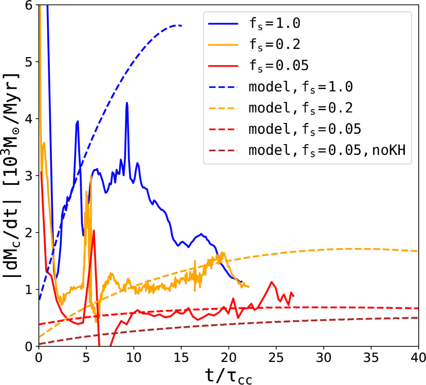
Figure 7: The total mass loss rate as a function of time for three simulations with varying thermal conduction efficiencies. The $\chi 300v1700$, $\chi 300v1700c5$ and $\chi 300v1700c20$ simulations are shown in blue, orange and red, respectively. Here we compare the solid lines from the simulations to the dashed lines from our model predictions. The brown dashed line shows the model prediction for the $\chi 300v1700c20$ simulation without considering mass loss from KHI. It is the only simulation where KHI plays a non-negligible role while the other simulations have $R_{\mathrm{c}}\ll\lambda_{\mathrm{KH}}$. The $\chi 300v1700c5$ and the $\chi 300v1700c20$ simulations are terminated at $t_{\mathrm{50}}$ and $t_{\mathrm{75}}$, respectively.

Figure 7 demonstrates how lowering the efficiency of thermal conduction affects the mass loss rate. Since the cloud in the $\chi 300v1700c5$ and the $\chi 300v1700c20$ simulations evaporates very slowly, we terminate those simulations at $t_{\mathrm{50}}$ and $t_{\mathrm{75}}$, respectively. In the first $\tau_{\mathrm{cc}}$, there is some mass loss during the cloud shock in each simulation, which our model does not attempt to capture. Afterwards, our model agrees with the low-conduction simulations very well and also agrees with the $\chi 300v1700$ well before $t_{\mathrm{50}}=9.19\tau_{\mathrm{cc}}$. After $t_{\mathrm{50}}$, the cloud in the $\chi 300v1700$ simulation starts to break into clumps, shortening $L_{\mathrm{c}}$ and lowering the total mass loss rate as a result. Since our model always assumes that the cloud is coherent, the mass loss rate from our model continues to grow with time as the cloud expands. In fact, for the same reason, we always over-estimate the late time mass loss in other simulations as well.

To first order, Equation 37 suggests that the mass loss rate scales linearly with the heat flux, so that reducing $f_{\mathrm{s}}$ will also reduce $\dot{M}_{\mathrm{c}}$ by the same factor. Moreover, reducing $f_{\mathrm{s}}$ changes the jump conditions at the bow shock, which determines the post-shock gas properties. When $f_{\mathrm{s}}$ is small enough, however, KHI will also start to cause additional mass loss and fragmentation in the cloud. This is indicated by comparing the red dashed line to the brown dashed line in Figure 7. The $\chi 300v1700c20$ simulation is the only one with $R_{\mathrm{c}}\sim\lambda_{\mathrm{KH}}$ so that KHI causes a noticeable fraction of the mass loss.

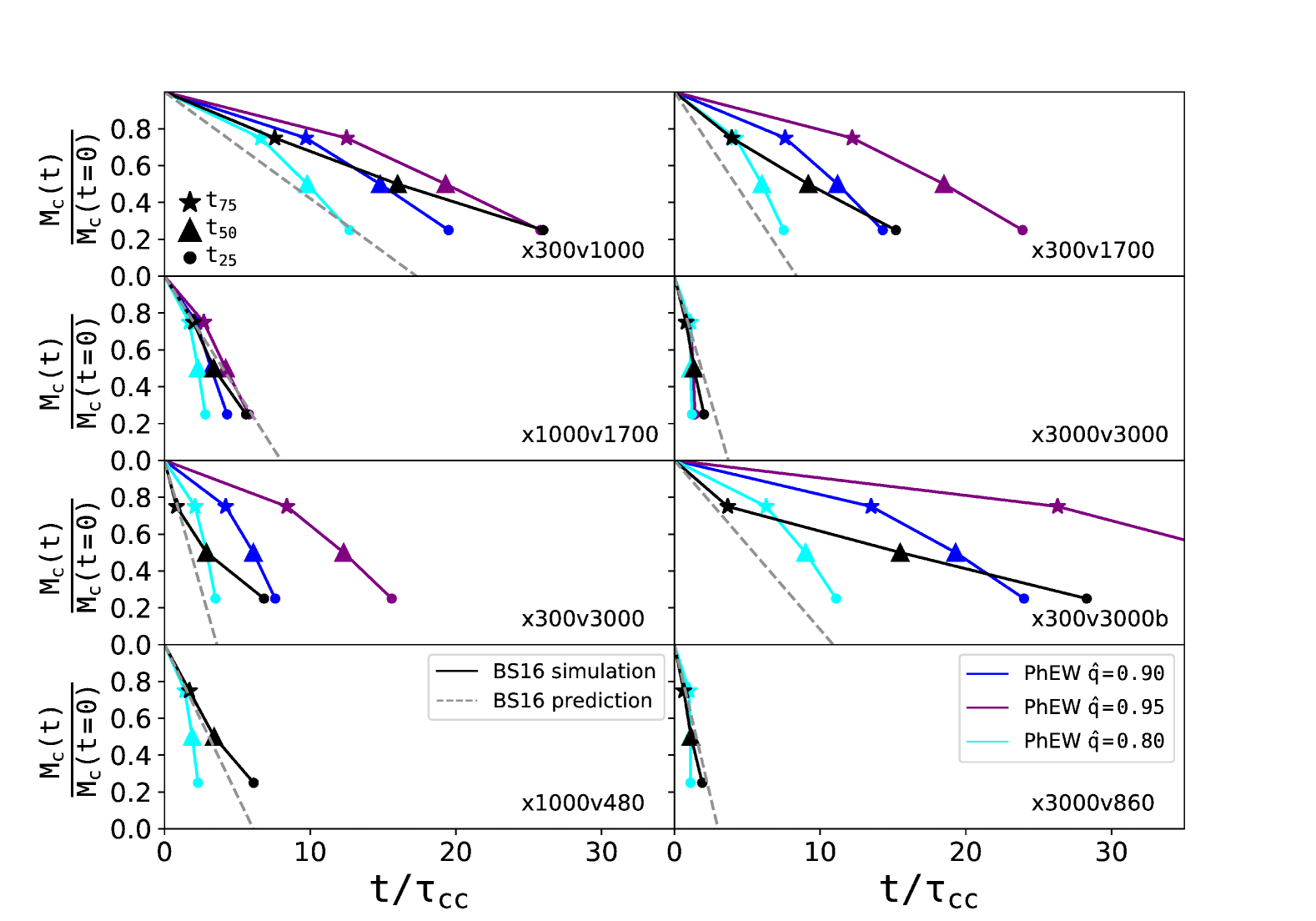
Figure 8: Same as Figure 6, except that we show model predictions with three different $\hat{q}_{\mathrm{s}}$. Increasing $\hat{q}_{\mathrm{s}}$ results in cooler post-shock gas and less evaporation in general. The two simulations in the bottom panels are not affected by changing $\hat{q}_{\mathrm{s}}$ because $\mathcal{M}_{1}=1$ in these simulations.

Figure 8 shows how sensitive the mass loss rate is to the $\hat{q}_{\mathrm{s}}$ parameter. At a constant Mach number, increasing $\hat{q}_{\mathrm{s}}$ reduces the post-shock temperature and increases the post-shock density (Figure 3). As a net effect, evaporation is less efficient with larger $\hat{q}_{\mathrm{s}}$ as thermal conduction primarily depends on the temperature. Even though we always assume a constant $\hat{q}_{\mathrm{s}}$ in our model, it actually evolves with time. The broadening of the front shock and conduction between the shock and the cloud tends to increase $\hat{q}_{\mathrm{s}}$, making the shock more isothermal over time. However, we do not attempt to include this behaviour in our model, as we consider the model sufficiently accurate for our purposes.

5.3 Velocity Evolution

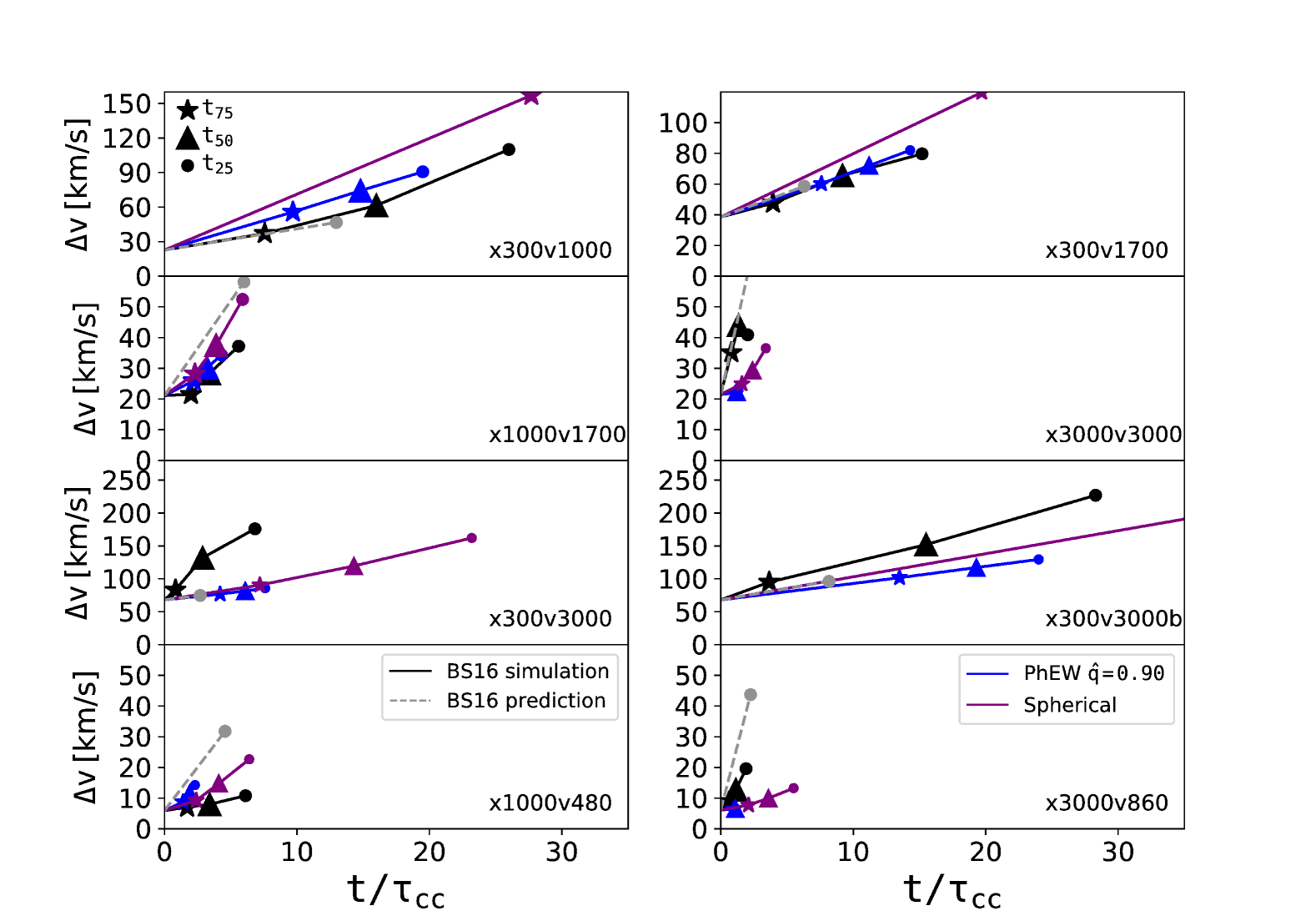
Figure 9: The evolution of the velocity of the cloud as a function of time. In each panel, we compare model predictions $\Delta_{v}(t)+v_{s}/3$ to the cloud speed measured from simulations. Stars, triangles and circles indicate values at $t_{\mathrm{75}}$, $t_{\mathrm{50}}$, $t_{\mathrm{25}}$ as in Figure 6. The predictions from our fiducial cylindrical model with $\hat{q}_{\mathrm{s}}=0.90$ and the spherical model are shown in blue and purple, respectively. Black symbols show results from the simulations (BS16). Grey dashed lines show their analytic predictions for velocity evolution (their equation 23).

Figure 9 shows how the cloud’s speed evolves with time. We define $\Delta v(t)$ as the difference between the average velocity of the cloud at any time $t$ after the cloud shock and the cloud velocity immediately after the cloud shock. In our models, $\Delta v(t)$ is governed solely by Equation 44, with $\Delta v(t=0)=0$ right after the cloud shock by definition.

In the simulations, the cloud gains momentum from the cloud shock. To make fair comparisons between the model predicted $\Delta v$ and the cloud speed measured from the simulations, we calculate how much velocity the cloud gains during the cloud shock and add it to $\Delta v$. As an approximation, we set this initial velocity to $(\pi/8)v_{s}$, where $v_{s}$ is the shock velocity calculated by assuming a pressure-driven plane-parallel cloud shock. The factor $\pi/8$ comes from the fact that the cloud shock is not exactly plane-parallel to the cloud. Instead, the front half of the cloud is compressed by shocks from all sides that ultimately converge. We calculate the net momentum that the cloud gains from the cloud shock in the direction of the flow as

$$\frac{1}{2}(2\pi\int_{0}^{R_{\mathrm{c}}}\int_{0}^{\pi}\rho_{3}v_{s}\sin\theta r^{2}\sin\theta drd\theta)=\frac{\pi}{8}M_{\mathrm{c}}v_{s},$$ (46)

where $\theta$ is the angle between the radial direction of the cloud and the polar direction, which is the direction that is perpendicular to the flow. The constant factor $1/2$ takes into account the fact that only the front half of the cloud gains momentum from shocks.

Despite the uncertainties in the systematic offset, the velocity evolution from our models agrees very well with the simulation results. The slope, which corresponds to the deceleration rate, is well reproduced for most cases. The success of modelling the deceleration relies on correctly calculating the ram pressure $P_{\mathrm{ram}}$ and the cloud radius $R_{\mathrm{c}}$, according to Equation 44. The ram pressure is robustly determined by the shock jump condition and is much less sensitive to the choice of $\hat{q}_{\mathrm{s}}$ than density or temperature. Therefore, correctly evolving $R_{\mathrm{c}}$, and thus the cross-section for ram pressure, is key to predicting the velocity evolution. It is crucial that we calculate $R_{\mathrm{c}}$ assuming cylindrical geometry and allow it to change only with $M_{\mathrm{c}}$ according to Equation 42. The spherical models slightly over-estimate the deceleration rate in most cases because of their relatively larger $R_{\mathrm{c}}$, according to Equation 45.

BS16 also calculate the velocity evolution of the clouds (their equation 22 and 23). We show their results in dashed lines in Figure 9. Their predictions for the cloud velocities are very similar to ours and agree with simulations equally well, even though their derivation for the velocities is very different from ours. As discussed above, this agreement between our calculations further indicates that the velocity evolution of the cloud depends critically on a few quantities such as $R_{\mathrm{c}}$ and $P_{\mathrm{ram}}$ that can be robustly computed.

6 Summary and Discussion

Hydrodynamic simulations of galaxy formation often employ sub-grid kinetic wind models to model feedback from star forming galaxies, however, none of the current simulations robustly evolve the outflowing wind material after they leave their host galaxies and enter into the CGM/IGM. In this paper, we propose an analytic model (Physically Evolved Winds; PhEW) that calculates how cold clouds that are launched with galactic winds evolve and propagate in such environments. We develop our analytic model based on findings from high resolution cloud-crushing simulations with (SB15) or without including isotropic thermal conduction (BS16) that simulate cold dense clouds travelling supersonically through a hot ambient medium.

These simulations suggest that thermal conduction plays a critical role in cloud evolution. BS16 shows that strong thermal conduction changes the shock jump conditions, suppresses KHI, confines the cloud into a cylindrical geometry, and evaporates the cloud. Therefore, we build our model in two separate scenarios, depending on whether or not thermal conduction dominates. When thermal conduction is insignificant, our model predicts mass loss rates according to the empirical scaling relations from the non-conductive simulations of SB15. Using these results for guidance, we self-consistently solve for the properties of the bow shock, the cloud shock and the evolution of the cloud. Since the strength of thermal conduction is very sensitive to temperature, real wind-CGM interactions in the Universe very likely fall into either of these scenarios. Nevertheless, we use a continuous but sharp transition from KHI-dominated mass loss to evaporation-dominated mass loss.

The PhEW model in thermal conduction dominated scenarios is able to predict the mass loss rate and the deceleration rate of the cloud at any time. These predictions agree with simulation results except for systems where thermal conduction is very saturated. We also find that a model that assumes that the clouds are spheres with uniform density significantly under-estimates the mass loss rate unless the evaporation timescale is comparable to $\tau_{\mathrm{cc}}$.

In addition to the simulations from BS16, we performed two simulations with reduced thermal conduction efficiency ($1/5$ and $1/20$ of the Spitzer rate) to $t_{\mathrm{75}}$. We find that even with much weaker thermal conduction, the KHI is still suppressed for very long times, consistent with the findings of Marcolini et al. (2005), where the cloud does not undergo any significant fragmentation for $f_{\mathrm{s}}=1/25$. The clouds in these simulations survive much longer because of their lower conductive evaporation rate. In the PhEW model, the KHI is nearly completely suppressed when $f_{\mathrm{s}}=1/5$ and is only partially suppressed when $f_{\mathrm{s}}=1/20$. Despite this difference, the PhEW model reproduces the mass loss rate of both clouds very well.

Many problems in galaxy formation struggle to have cold clouds survive sufficiently long in a hot medium. For example, entrainment of cold gas in supernova remnants has been proposed as a mechanism to generate galactic winds, but it is often found that the clouds disrupt too fast to be accelerated to wind velocities. Even after they are able to leave the galaxy, their subsequent evolution in the hot CGM is significantly limited by how fast they disintegrate. In BS16, most clouds evaporate on a few $\tau_{\mathrm{cc}}$, or a few Myrs, a timescale too short to be important for galaxy formation. Even the cloud that survives the longest can travel no more than $50\ \mathrm{kpc}$, a distance that is much shorter than the virial radius of massive, hot haloes. Furthermore, the initial mass of the cloud in their simulations is $6.7\times 10^{4}M_{\odot}$, which is likely much larger than an average cloud in the CGM. Since smaller clouds evaporate faster under the same physical conditions, the cloud survival problem becomes even more severe than that suggested by the BS16 simulations.

Our findings on the effects of lowering thermal conduction efficiency suggest that one may significantly lengthen the lifetime of clouds by keeping the thermal conduction very weak yet still strong enough to suppress hydrodynamic instabilities and keep the cloud structure coherent. For example, suppressing thermal conduction by a factor of 10 will in principle help the cloud survive nearly 10 times longer and hence travel much further into the galactic halo.

Neither the BS16 simulations nor our models explicitly include magnetic fields, even though an important consequence of adding magnetic field is suppression of thermal conduction. Strong magnetic fields are known to also suppress hydrodynamic instabilities and significantly affect the geometry and lifetimes of clouds (Mac Low et al., 1994; Orlando et al., 2008; McCourt et al., 2015), though Cottle et al. (2020) suggest that magnetic draping does not significantly enhance cloud lifetime. Even a very weak magnetic field as probable in the CGM could strongly affect cloud evolution depending on the alignment between the flow and the field (Li et al., 2019; Cottle et al., 2020). However, our understanding of the properties and the effects of magnetic fields in the CGM is still very poor. Even though we do not explicitly model a magnetic field, we may capture its effects by varying the parameters $f_{\mathrm{KH}}$ and $f_{\mathrm{s}}$, which are, in reality, affected by the magnetic field.

It is straightforward to implement the PhEW model into hydrodynamic simulations of galaxy formation that employ kinetic feedback. In simulations that use a particle-based hydrodynamic method, e.g., smoothed particle hydrodynamic (SPH) simulations (Springel, 2010), a common practice of modelling galactic winds is by statistically ejecting gas particles from galaxies (Springel & Hernquist, 2003; Oppenheimer & Davé, 2006; Huang et al., 2020). The wind algorithm in each simulation determines the initial velocity of the ejected particles (wind particles) often as a function of their host galaxy properties. In some simulations, the wind particles temporarily decouple from the other SPH particles hydrodynamically after launch but soon recouple to the hydrodynamics when the re-coupling criteria are satisfied. After re-coupling, their evolution is again governed by the SPH equations as for a normal gas particle.

In the PhEW model, one would launch the wind particle and let it evolve as before during the decoupling phase. Once it meets the original re-coupling criteria, one would start evolving it as a PhEW particle instead of letting it recouple. One could consider a PhEW particle of mass $m_{\mathrm{i}}$ as a collection of $N_{\mathrm{i}}$ identical cold clouds, each of them having an initial mass $M_{\mathrm{c}}$. The cloud mass $M_{\mathrm{c}}$ is a free parameter of the model but by mass conservation, $m_{\mathrm{i}}=N_{\mathrm{i}}M_{\mathrm{c}}$.

The choice of $M_{\mathrm{c}}$ affects both the velocity evolution of the cloud and the mass loss rate. Under pressure equilibrium, $R_{\mathrm{c}}$ scales with $M_{\mathrm{c}}^{1/3}$ so that the deceleration rate scales as $\dot{v}_{\mathrm{rel}}\propto M_{\mathrm{c}}^{-1/3}$ (Equation 44). When the KHI dominates the mass loss, $\tau_{\mathrm{KH}}\propto\tau_{\mathrm{cc}}\propto M_{\mathrm{c}}^{1/3}$. When evaporation dominates the mass loss, the evaporation time-scale $\tau_{\mathrm{ev}}\propto M_{\mathrm{c}}/R_{\mathrm{c}}\sim M_{\mathrm{c}}^{2/3}$. Therefore, increasing the cloud mass $M_{\mathrm{c}}$ helps clouds survive longer. Together with $f_{\mathrm{KH}}$ and $f_{\mathrm{s}}$, these parameters control the evolution of PhEW particles in cosmological simulations.

To apply our PhEW model (Section 4.1) to the clouds, one would first evaluate the density $\rho_{1}$ and temperature $T_{1}$ of their surroundings and the relative velocity $v_{\mathrm{rel}}$. In SPH simulations, this is conveniently done by performing a kernel weighted average over the neighbouring SPH particles. We would choose a time-step for the PhEW particle to that required for accurate integration. At each time-step, one would calculate the amount of mass (along with the metals), momentum, and energy lost since the last timestep and deposit it into the neighbouring SPH particles in a kernel weighted fashion. At the same time, one would reduce the mass and the velocity of the PhEW particle accordingly.

As a PhEW particle travels away from the galaxy into the less dense CGM/IGM, it will gradually expand in the radial direction and could heat up as well. These long-term behaviours are not modelled in the analytic model presented above but would need to be captured in cosmological simulations. In practice, one would allow the cloud radius to adjust with the ram pressure $P_{\mathrm{ram}}$ in the simulation and maintain pressure balance at the head of the cloud, i.e., $P_{\mathrm{ram}}=n_{\mathrm{c}}k_{\mathrm{B}}T_{\mathrm{c}}$. One would obtain the cloud radius under pressure equilibrium at any time using Equation 42:

$$R_{\mathrm{c,peq}}=\left(\frac{\gamma M_{\mathrm{c}}}{\pi P_{\mathrm{ram}}L_{\mathrm{c}}}\right)^{1/2}c_{\mathrm{c}}.$$ (47)

At each time-step $\Delta t$, one would let the cloud radius adjust on a sound-crossing time-scale, i.e., $\tau_{\mathrm{sc}}\equiv R_{\mathrm{c}}/c_{\mathrm{c}}$:

$$R_{\mathrm{c}}(t+\Delta t)=R_{\mathrm{c,peq}}+(R_{\mathrm{c}}-R_{\mathrm{c,peq}})\exp\left(-\frac{\Delta t}{\tau_{\mathrm{sc}}}\right).$$ (48)

The work done by the cloud in $\Delta t$ during expansion is approximately:

$$W_{\mathrm{exp}}=2\pi P_{\mathrm{ram}}c_{\mathrm{c}}\left[R_{\mathrm{c}}+2(R_{\mathrm{c,peq}}-R_{\mathrm{c}})\frac{\Delta t}{\tau_{\mathrm{sc}}}\right]\Delta t,$$ (49)

which, along with the cooling and heating rate of the cloud, determines how the internal energy of the cloud changes over time.

A PhEW particle may eventually recouple if either of the following happens. First, it has lost over 90% of its original mass. In this case one would remove the particle from simulation and deposit its remaining mass and momentum in the neighbouring particles. Second, the clouds become similar enough to the ambient medium, i.e., $\rho_{4}\sim\rho_{1}$, $T_{4}\sim T_{1}$ and $v_{\mathrm{rel}}<c_{1}$. Third, the particle crosses a galaxy in its path. In this case, which can happen in a cosmological simulation, the physics of PhEW would break down so we let the particle recouple and become a normal gas particle. We will describe the mathematical details of this implementation in future work.

Similarly, one can combine the PhEW model with grid-based simulations. For example, the Illustris TNG simulations (Vogelsberger et al., 2013; Pillepich et al., 2018a) model galactic winds by temporarily turning a cell into a particle that decouples from hydrodynamics until re-coupling. To apply the PhEW model to the wind particle, one would first track the cell where the particle is located at each time-step. Then we could use the cell properties as the ambient and exchange mass as well as other conserved quantities between the particle and the cell. Finally one would recouple the particle to the grid similarly as in the SPH implementation.

In summary, we developed an analytic model, PhEW, that calculates the evolution of individual clouds over a wide range of physical conditions that reproduces very high resolution simulations of individual clouds. This model can be implemented into hydrodynamic simulations of galaxy formation and will provide a more robust way of evolving cold galactic outflows in galactic haloes of various properties. The PhEW model explicitly models physical processes that occur at gas interfaces such as bow shocks, hydrodynamic instabilities, fluid mixing and thermal conduction. The PhEW model has a few parameters such as the mass of individual clouds, the Kelvin-Helmholtz coefficient $f_{\mathrm{KH}}$ and the thermal conduction coefficient $f_{\mathrm{s}}$ that affect the properties and the evolution of the clouds. Including these under-resolved and often neglected processes in galaxy formation simulations will be a crucial step towards a more realistic and controlled interpretation of the observations of multi-phase gas sub-structures in the circumgalactic medium within the framework of galaxy formation and evolution. We will present the results of including this model in a GIZMO (Hopkins, 2015) based cosmological simulation (Davé et al., 2019) in a future paper.

Data availability

The data underlying this article will be shared on reasonable request to the corresponding author.

Appendix A Nomenclature

We list the main variables used in this paper here.

Flow properties in the cloud-crushing problem.
$\rho_{1}$, $T_{1}$, $P_{1}$ - density, temperature and pressure of the pre-shock ambient flow
$\rho_{3}$, $T_{3}$, $P_{3}$ - density, temperature and pressure of the cloud before the cloud shock
$\chi_{0}$ - initial density ratio between the cloud and the ambient medium
$v_{\mathrm{rel}}$ - relative velocity between the cloud and the ambient medium
$c_{\mathrm{s,1}}$ - sound speed of the pre-shock ambient flow
$\mathcal{M}_{1}$ - Mach number of the ambient flow relative to the cloud
$M_{\mathrm{c}}$ - cloud mass
$x$ - coordinate in the cloud along the long axis, with x = 0 at the cloud head
$\chi$ - density ratio between the cloud and the ambient medium
$n_{\mathrm{c}}$, $n_{4}$ - hydrogen number density of the cloud
$\rho_{\mathrm{c}}$, $\rho_{4}$ - cloud density at the cloud head, i.e., short for $\rho_{4}(0)$
$P_{\mathrm{c}}$, $P_{4}$ - internal pressure at the cloud head, i.e., short for $P_{4}(0)$
$T_{\mathrm{c}}$, $T_{4}$ - cloud temperature
$T_{\mathrm{eq}}$ - cloud temperature at thermal equilibrium between radiative cooling and heating
$c_{\mathrm{c}}$ - sound speed inside the cloud
$R_{\mathrm{c}}$ - cloud radius perpendicular to direction of motion
$R_{\mathrm{c,peq}}$ - cloud radius under pressure equilibrium
$L_{\mathrm{c}}$ - cloud length along direction of motion
$P_{\mathrm{ram}}$ - ram pressure ahead of the cloud
$P_{\mathrm{II}}$ - pressure at the contact point II, which is equal to the ram pressure
$P_{\mathrm{ev}}$ - vapour pressure owing to evaporation
$v_{\mathrm{exp}}$ - expansion velocity of the cloud
$r_{\mathrm{II}}$ - radius of the streamline that is arbitrarily chosen as the outer boundary of the conduction zone in the post-shock flow
$u_{\mathrm{II}}$ - velocity along the streamline
$n_{\mathrm{II}}$ - hydrogen number density along the streamline
$\rho_{\mathrm{II}}$ - density along the streamline
$T_{\mathrm{II}}$ - temperature along the streamline
$c_{\mathrm{II}}$ - sound speed along the streamline

Properties of the bow shock and the cloud shock.
$v_{s}$ - velocity of the cloud shock
$\rho_{\mathrm{a}}$ - density of the pre-shock gas
$T_{\mathrm{a}}$ - temperature of the pre-shock gas
$\rho_{\mathrm{ps}}$ - density of the post-shock gas
$T_{\mathrm{ps}}$ - temperature of the post-shock gas
$\eta_{\mathrm{s}}$ - correction factor for the density jump across a conductive shock
$\tau_{\mathrm{s}}$ - correction factor for the temperature jump across a conductive shock

Thermal conduction.
$n_{\mathrm{h}}$ - hydrogen number density in the hot gas in a two-phase medium
$\rho_{\mathrm{h}}$ - gas density in the hot gas in a two-phase medium
$T_{\mathrm{h}}$ - temperature of the hot gas in a two-phase medium
$c_{\mathrm{h}}$ - sound speed of the hot gas in a two-phase medium
$\mathcal{M}_{\mathrm{h}}$ - Mach number of the hot gas in a two-phase medium
$\lambda_{\mathrm{mfp}}$ - mean free path of electrons in the hot medium
$q_{\mathrm{class}}$ - classical heat flux from thermal conduction
$q_{\mathrm{sat}}$ - saturated heat flux from thermal conduction
$\sigma_{0}$ - conductive coefficient, defined as the ratio between the classical and the saturated heat flux
$\sigma_{\mathrm{c}}$ - conductive coefficient at the cloud surface
$\tau_{\mathrm{ev,class}}$ - time-scale for classical evaporation from CM77
$\tau_{\mathrm{ev,sat}}$ - time-scale for saturated evaporation from CM77

The conduction zone.
$\mathcal{M}_{\mathrm{sat}}$ - Mach number in the saturated zone
$r_{*}$ - radius of the transition point where thermal conduction saturates
$n_{*}$ - hydrogen number density at the transition point
$\rho_{*}$ - density at the transition point
$T_{*}$ - temperature at the transition point
$q_{*}$ - Heat flux at the transition point

Mass loss rates.
$\dot{\hat{m}}_{\mathrm{A}}$ - mass loss rate per unit area owing to conductive evaporation on the cloud surface
$\dot{M}_{\mathrm{c,KH}}$ - total mass loss rate from KHI
$\dot{M}_{\mathrm{c,ev}}$ - total mass loss rate from conductive evaporation
$\dot{M}_{\mathrm{c}}$ - total mass loss rate of the cloud from both KHI and conductive evaporation

Various scales.
$\tau_{\mathrm{sc}}$ - sound crossing time-scale
$\tau_{\mathrm{cc}}$ - cloud-crushing time-scale
$\tau_{\mathrm{diff}}$ - diffusion time-scale owing to thermal conduction
$\tau_{\mathrm{mix}}$ - mixing time-scale owing to Kelvin-Helmholtz instability
$\tau_{\mathrm{KH}}$ - Kelvin-Helmholtz time-scale
$\lambda_{\mathrm{KH}}$ - Kelvin-Helmholtz scale. Perturbations on scales below it are suppressed by thermal conduction
$L_{\mathrm{F}}$ - Field length

Parameters and fixed-value factors.
$f_{\mathrm{s}}$ - parameter that determines the efficiency of thermal conduction. $f_{\mathrm{s}}=1$ corresponds to conduction at the Spitzer value.
$f_{\mathrm{KH}}$ - parameter that determines the general growth of Kelvin-Helmholtz instability mass loss
$\hat{q}_{\mathrm{s}}$ - the ratio between the heat flux and the kinetic energy flow across a conductive shock front, approximated as 0.90 in this paper
$f_{\mathrm{ram}}$ - factor that affects the ram pressure according to Equation 10, approximated as 0.5 in this paper
$f_{\mathrm{r}}$ - factor defined as $f_{\mathrm{r}}\equiv\ln(r_{\mathrm{II}}/R_{\mathrm{c}})$, approximated as 1.0 in this paper
$f_{\mathrm{m}}$ - factor that affects the total evaporation rate according to Equation 37, approximated as 3.5 in this paper

Appendix B Modified Shock Jump Conditions

The Rankine-Hugoniot jump conditions relate post-shock gas properties to the pre-shock gas properties across an adiabatic, non-conductive plane-parallel shock. When thermal conduction is efficient, the shock front will be smoothed by the enthalpy flow in the upstream direction. The jump conditions can be obtained by considering that fluid quantities are conserved across the shock:

$$\rho_{1}v_{1}=\rho_{2}v_{2},$$ (50)

$$\rho_{1}v_{1}^{2}+P_{1}=\rho_{2}v_{2}^{2}+P_{2},$$ (51)

and

$$\frac{1}{2}\rho_{1}v_{1}^{3}+\frac{5}{2}P_{1}v_{1}=\frac{1}{2}\rho_{2}v_{2}^{3}+\frac{5}{2}P_{2}v_{2}+q_{s},$$ (52)

where, following the notation of Borkowski et al. (1989), we introduce dimensionless parameters $\eta_{\mathrm{s}}\equiv\rho_{2}/(4\rho_{1})$, $\tau_{\mathrm{s}}\equiv 16k_{\mathrm{B}}T/(3\mu m_{\mathrm{H}}v_{1}^{2})$, and $\hat{q}_{\mathrm{s}}\equiv q_{s}/(\rho_{1}v_{1}^{3}/2)$.

Equations 50 to 52 are identical to equations (8) to (10) in Borkowski et al. (1989) except for the pre-shock terms $P_{1}$ and $5P_{1}v_{1}/2$ that are ignored in their paper. Even though $P_{2}\gg P_{1}$ in equations 51 and 52, $P_{1}v_{1}/P_{2}v_{2}\sim T_{1}/T_{2}$ is not necessarily infinitesimal, unless the shock mach number $\mathcal{M}\gg 1$. Therefore, including these two terms, especially the second, should largely improve the accuracy in low Mach number shocks.

Solving these equations we obtain:

$$\eta_{\mathrm{s}}=\frac{5(1+\beta_{\mathrm{s}})+\sqrt{9+16\hat{q}_{\mathrm{s}}+5\beta_{\mathrm{s}}(5\beta_{\mathrm{s}}-6)}}{8(1-\hat{q}_{\mathrm{s}}+5\beta_{\mathrm{s}})},$$ (53)

and

$$\tau_{\mathrm{s}}=\frac{1}{2}-\frac{4\hat{q}_{\mathrm{s}}}{3}+\frac{1}{6}(1+\beta_{\mathrm{s}})\sqrt{9+16\hat{q}_{\mathrm{s}}+5\beta_{\mathrm{s}}(5\beta_{\mathrm{s}}-6)}+\frac{5}{6}\beta_{\mathrm{s}}(\beta_{\mathrm{s}}+6),$$ (54)

which immediately yields Equations 12 and 13 in the text.

Appendix C Integrals

To integrate Equation 37 one needs to know the mass loss rate per area, $\dot{\hat{m}}_{\mathrm{A}}$, at each point along the cloud, which in turn relies on the properties of the ambient flow. We relate each point along the cloud to another point on the streamline (noted as boundary II in Figures 1 and 4) in the ambient flow. Along the streamline, fluid properties are parameterised by flow velocity according to Bernoulli’s equations:

$$\frac{\rho_{\mathrm{II}}(0)}{\rho_{\mathrm{II}}(x)}=\left(1-\frac{\gamma-1}{2}\frac{u_{\mathrm{II}}^{2}(x)}{c_{\mathrm{II}}^{2}(x)}\right)^{\frac{1}{\gamma-1}},$$ (55)

$$\frac{P_{\mathrm{II}}(0)}{P_{\mathrm{II}}(x)}=\left(1-\frac{\gamma-1}{2}\frac{u_{\mathrm{II}}^{2}(x)}{c_{\mathrm{II}}^{2}(x)}\right)^{\frac{\gamma}{\gamma-1}},$$ (56)

and

$$\frac{T_{\mathrm{II}}(0)}{T_{\mathrm{II}}(x)}=1-\frac{\gamma-1}{2}\frac{u_{\mathrm{II}}^{2}(x)}{c_{\mathrm{II}}^{2}(x)},$$ (57)

where $u_{\mathrm{II}}(x)$ and $c_{\mathrm{II}}(x)$ are the flow speed and the sound speed at the point on the streamline that corresponds to coordinate $x$ in the cloud. The cloud head at $x=0$ corresponds to the stagnation point where $u_{\mathrm{II}}=0$.

To simplify the integral, we assume that

$$\frac{dx}{du_{\mathrm{II}}^{2}}=\frac{x}{u_{\mathrm{II}}^{2}}.$$ (58)

Also, we assume that at the tail of the cloud $x=L_{\mathrm{c}}\gg R_{\mathrm{c}}$, the ambient flow becomes identical to the unperturbed flow: $T_{\mathrm{II}}(L_{\mathrm{c}})=T_{1}$, $c_{\mathrm{II}}(L_{\mathrm{c}})=c_{1}$.

Combining Equation 57 and Equation 58:

$$\begin{split}dx&=\left(\frac{L_{\mathrm{c}}}{u_{\mathrm{II}}^{2}(L_{\mathrm{c}})}\right)du_{\mathrm{II}}^{2}\\ &=\left[\frac{(\gamma-1)L_{\mathrm{c}}}{2c_{1}}\left(1-\frac{T_{1}}{T_{\mathrm{II}}(0)}\right)^{-1}\right]du_{\mathrm{II}}^{2}\\ &=-L_{\mathrm{c}}\left(1-\frac{T_{1}}{T_{\mathrm{II}}(0)}\right)^{-1}\frac{dT}{T_{\mathrm{II}}(0)}\\ &=-L_{\mathrm{c}}\frac{dT}{T_{\mathrm{II}}(0)-T_{1}}\end{split}$$ (59)

Therefore, assuming classical conduction, the integral governing the total mass loss rate becomes:

$$\begin{split}\int_{0}^{L_{\mathrm{c}}}\dot{\hat{m}}_{\mathrm{A}}(x)dx&=A(T_{1},T_{\mathrm{II}}(0),R_{\mathrm{c}})\frac{L_{\mathrm{c}}}{T_{\mathrm{II}}(0)-T_{1}}\int_{T_{1}}^{T_{\mathrm{II}}(0)}T^{5/2}dT\\ &\sim\frac{1}{3.5}A(T_{1},T_{\mathrm{II}}(0),R_{\mathrm{c}})L_{\mathrm{c}}\frac{T_{\mathrm{II}}(0)^{7/2}-T_{1}^{7/2}}{T_{\mathrm{II}}(0)-T_{1}}\\ &=\frac{1}{3.5}\left[\frac{1-\left(\frac{T_{1}}{T_{\mathrm{II}}(0)}\right)^{3.5}}{1-\left(\frac{T_{1}}{T_{\mathrm{II}}(0)}\right)}\right]L_{\mathrm{c}}\dot{\hat{m}}_{\mathrm{A}}(0)\end{split}.$$ (60)

Comparing the above results to Equation 37 indicates $f_{\mathrm{m}}=3.5$ when $T_{\mathrm{II}}(0)\gg T_{1}$.

References

- Anderson et al. (2013) Anderson M. E., Bregman J. N., Dai X., 2013, ApJ, 762, 106
- Armillotta et al. (2016) Armillotta L., Fraternali F., Marinacci F., 2016, MNRAS, 462, 4157
- Armillotta et al. (2017) Armillotta L., Fraternali F., Werk J. K., Prochaska J. X., Marinacci F., 2017, MNRAS, 470, 114
- Balbus & McKee (1982) Balbus S. A., McKee C. F., 1982, ApJ, 252, 529
- Banda-Barragán et al. (2019) Banda-Barragán W. E., Zertuche F. J., Federrath C., García Del Valle J., Brüggen M., Wagner A. Y., 2019, MNRAS, 486, 4526
- Begelman & McKee (1990) Begelman M. C., McKee C. F., 1990, ApJ, 358, 375
- Benson et al. (2003) Benson A. J., Bower R. G., Frenk C. S., Lacey C. G., Baugh C. M., Cole S., 2003, ApJ, 599, 38
- Bogdán et al. (2013) Bogdán Á., Forman W. R., Kraft R. P., Jones C., 2013, ApJ, 772, 98
- Bogdán et al. (2017) Bogdán Á., Bourdin H., Forman W. R., Kraft R. P., Vogelsberger M., Hernquist L., Springel V., 2017, ApJ, 850, 98
- Borkowski et al. (1989) Borkowski K. J., Shull J. M., McKee C. F., 1989, ApJ, 336, 979
- Brüggen & Scannapieco (2016) Brüggen M., Scannapieco E., 2016, ApJ, 822, 31
- Chandrasekhar (1961) Chandrasekhar S., 1961, Hydrodynamic and hydromagnetic stability
- Cottle et al. (2020) Cottle J., Scannapieco E., Bruggen M., Band a-Barragan W., Federrath C., 2020, arXiv e-prints, p. arXiv:2002.07804
- Cowie & McKee (1977) Cowie L. L., McKee C. F., 1977, ApJ, 211, 135
- Crighton et al. (2015) Crighton N. H. M., Hennawi J. F., Simcoe R. A., Cooksey K. L., Murphy M. T., Fumagalli M., Prochaska J. X., Shanks T., 2015, MNRAS, 446, 18
- Davé et al. (2013) Davé R., Katz N., Oppenheimer B. D., Kollmeier J. A., Weinberg D. H., 2013, MNRAS, 434, 2645
- Davé et al. (2019) Davé R., Anglés-Alcázar D., Narayanan D., Li Q., Rafieferantsoa M. H., Appleby S., 2019, MNRAS, 486, 2827
- Dekel et al. (2009) Dekel A., et al., 2009, Nature, 457, 451
- Field (1965) Field G. B., 1965, ApJ, 142, 531
- Fielding et al. (2017) Fielding D., Quataert E., Martizzi D., Faucher-Giguère C.-A., 2017, MNRAS, 470, L39
- Ford et al. (2013) Ford A. B., Oppenheimer B. D., Davé R., Katz N., Kollmeier J. A., Weinberg D. H., 2013, MNRAS, 432, 89
- Ford et al. (2016) Ford A. B., et al., 2016, MNRAS, 459, 1745
- Girichidis et al. (2016) Girichidis P., et al., 2016, MNRAS, 456, 3432
- Governato et al. (2007) Governato F., Willman B., Mayer L., Brooks A., Stinson G., Valenzuela O., Wadsley J., Quinn T., 2007, MNRAS, 374, 1479
- Grand et al. (2017) Grand R. J. J., et al., 2017, MNRAS, 467, 179
- Gronke & Oh (2018) Gronke M., Oh S. P., 2018, MNRAS, 480, L111
- Gupta et al. (2012) Gupta A., Mathur S., Krongold Y., Nicastro F., Galeazzi M., 2012, ApJ, 756, L8
- Gupta et al. (2017) Gupta A., Mathur S., Krongold Y., 2017, ApJ, 836, 243
- Hopkins (2015) Hopkins P. F., 2015, MNRAS, 450, 53
- Hopkins & Raives (2016) Hopkins P. F., Raives M. J., 2016, MNRAS, 455, 51
- Hopkins et al. (2012) Hopkins P. F., Quataert E., Murray N., 2012, MNRAS, 421, 3522
- Hopkins et al. (2014) Hopkins P. F., Kereš D., Oñorbe J., Faucher-Giguère C.-A., Quataert E., Murray N., Bullock J. S., 2014, MNRAS, 445, 581
- Huang et al. (2020) Huang S., Katz N., Davé R., Oppenheimer B. D., Weinberg D. H., Fardal M., Kollmeier J. A., Peeples M. S., 2020, MNRAS, 493, 1
- Hummels et al. (2019) Hummels C. B., et al., 2019, ApJ, 882, 156
- Kereš et al. (2005) Kereš D., Katz N., Weinberg D. H., Davé R., 2005, MNRAS, 363, 2
- Kereš et al. (2009) Kereš D., Katz N., Fardal M., Davé R., Weinberg D. H., 2009, MNRAS, 395, 160
- Kim & Ostriker (2017) Kim C.-G., Ostriker E. C., 2017, ApJ, 846, 133
- Klein et al. (1994) Klein R. I., McKee C. F., Colella P., 1994, ApJ, 420, 213
- Lacey (1988) Lacey C. G., 1988, ApJ, 326, 769
- Lan & Mo (2019) Lan T.-W., Mo H., 2019, MNRAS, 486, 608
- Landau & Lifshitz (1959) Landau L. D., Lifshitz E. M., 1959, Fluid mechanics
- Li et al. (2017) Li M., Bryan G. L., Ostriker J. P., 2017, ApJ, 841, 101
- Li et al. (2019) Li Z., Hopkins P. F., Squire J., Hummels C., 2019, arXiv e-prints, p. arXiv:1909.02632
- Mac Low et al. (1994) Mac Low M.-M., McKee C. F., Klein R. I., Stone J. M., Norman M. L., 1994, ApJ, 433, 757
- Mandelker et al. (2016) Mandelker N., Padnos D., Dekel A., Birnboim Y., Burkert A., Krumholz M. R., Steinberg E., 2016, MNRAS, 463, 3921
- Mandelker et al. (2019) Mandelker N., van den Bosch F. C., Springel V., van de Voort F., 2019, ApJ, 881, L20
- Marcolini et al. (2005) Marcolini A., Strickland D. K., D’Ercole A., Heckman T. M., Hoopes C. G., 2005, MNRAS, 362, 626
- McCourt et al. (2015) McCourt M., O’Leary R. M., Madigan A.-M., Quataert E., 2015, MNRAS, 449, 2
- McCourt et al. (2018) McCourt M., Oh S. P., O’Leary R., Madigan A.-M., 2018, MNRAS, 473, 5407
- McKee & Cowie (1975) McKee C. F., Cowie L. L., 1975, ApJ, 195, 715
- Micono et al. (2000) Micono M., Bodo G., Massaglia S., Rossi P., Ferrari A., Rosner R., 2000, A&A, 360, 795
- Muratov et al. (2015) Muratov A. L., Kereš D., Faucher-Giguère C.-A., Hopkins P. F., Quataert E., Murray N., 2015, MNRAS, 454, 2691
- Murray et al. (2005) Murray N., Quataert E., Thompson T. A., 2005, ApJ, 618, 569
- Nelson et al. (2018) Nelson D., et al., 2018, MNRAS, 477, 450
- Oppenheimer & Davé (2006) Oppenheimer B. D., Davé R., 2006, MNRAS, 373, 1265
- Oppenheimer et al. (2010) Oppenheimer B. D., Davé R., Kereš D., Fardal M., Katz N., Kollmeier J. A., Weinberg D. H., 2010, MNRAS, 406, 2325
- Orlando et al. (2005) Orlando S., Peres G., Reale F., Bocchino F., Rosner R., Plewa T., Siegel A., 2005, A&A, 444, 505
- Orlando et al. (2008) Orlando S., Bocchino F., Reale F., Peres G., Pagano P., 2008, ApJ, 678, 274
- Peeples et al. (2014) Peeples M. S., Werk J. K., Tumlinson J., Oppenheimer B. D., Prochaska J. X., Katz N., Weinberg D. H., 2014, ApJ, 786, 54
- Peeples et al. (2019) Peeples M. S., et al., 2019, ApJ, 873, 129
- Pieri et al. (2014) Pieri M. M., et al., 2014, MNRAS, 441, 1718
- Pillepich et al. (2018a) Pillepich A., et al., 2018a, MNRAS, 473, 4077
- Pillepich et al. (2018b) Pillepich A., et al., 2018b, MNRAS, 475, 648
- Rossi et al. (1997) Rossi P., Bodo G., Massaglia S., Ferrari A., 1997, A&A, 321, 672
- Scannapieco & Brüggen (2015) Scannapieco E., Brüggen M., 2015, ApJ, 805, 158
- Schaye et al. (2015) Schaye J., et al., 2015, MNRAS, 446, 521
- Schneider & Robertson (2017) Schneider E. E., Robertson B. E., 2017, ApJ, 834, 144
- Schneider et al. (2018) Schneider E. E., Robertson B. E., Thompson T. A., 2018, ApJ, 862, 56
- Sparre et al. (2019) Sparre M., Pfrommer C., Vogelsberger M., 2019, MNRAS, 482, 5401
- Springel (2010) Springel V., 2010, ARA&A, 48, 391
- Springel & Hernquist (2003) Springel V., Hernquist L., 2003, MNRAS, 339, 312
- Steidel et al. (2010) Steidel C. C., Erb D. K., Shapley A. E., Pettini M., Reddy N., Bogosavljević M., Rudie G. C., Rakic O., 2010, ApJ, 717, 289
- Stern et al. (2016) Stern J., Hennawi J. F., Prochaska J. X., Werk J. K., 2016, ApJ, 830, 87
- Stinson et al. (2006) Stinson G., Seth A., Katz N., Wadsley J., Governato F., Quinn T., 2006, MNRAS, 373, 1074
- Stone et al. (1997) Stone J. M., Xu J., Hardee P., 1997, ApJ, 483, 136
- Tanner et al. (2016) Tanner R., Cecil G., Heitsch F., 2016, ApJ, 821, 7
- Thompson et al. (2016) Thompson T. A., Quataert E., Zhang D., Weinberg D. H., 2016, MNRAS, 455, 1830
- Tumlinson et al. (2011) Tumlinson J., et al., 2011, Science, 334, 948
- Tumlinson et al. (2017) Tumlinson J., Peeples M. S., Werk J. K., 2017, ARA&A, 55, 389
- Veilleux et al. (2020) Veilleux S., Maiolino R., Bolatto A. D., Aalto S., 2020, A&ARv, 28, 2
- Vieser & Hensler (2007) Vieser W., Hensler G., 2007, A&A, 472, 141
- Vietri et al. (1997) Vietri M., Ferrara A., Miniati F., 1997, ApJ, 483, 262
- Vogelsberger et al. (2013) Vogelsberger M., Genel S., Sijacki D., Torrey P., Springel V., Hernquist L., 2013, MNRAS, 436, 3031
- Wang et al. (2015) Wang L., Dutton A. A., Stinson G. S., Macciò A. V., Penzo C., Kang X., Keller B. W., Wadsley J., 2015, MNRAS, 454, 83
- Werk et al. (2014) Werk J. K., et al., 2014, ApJ, 792, 8
- White & Frenk (1991) White S. D. M., Frenk C. S., 1991, ApJ, 379, 52
- Xu et al. (2000) Xu J., Hardee P. E., Stone J. M., 2000, ApJ, 543, 161
- Yu et al. (2020) Yu B. P. B., Owen E. R., Wu K., Ferreras I., 2020, MNRAS, 492, 3179
- Zhang et al. (2017) Zhang D., Thompson T. A., Quataert E., Murray N., 2017, MNRAS, 468, 4801
- van de Voort et al. (2019) van de Voort F., Springel V., Mandelker N., van den Bosch F. C., Pakmor R., 2019, MNRAS, 482, L85