Understanding the MiniBooNE and the muon and electron $g-2$ anomalies with a light $Z^{\prime}$ and a second Higgs doublet

Abstract

Two of the most widely studied extensions of the Standard Model (SM) are $a)$ the addition of a new $U(1)$ symmetry to its existing gauge groups, and $b)$ the expansion of its scalar sector to incorporate a second Higgs doublet. We show that when combined, they allow us to understand the electron-like event excess seen in the MiniBooNE (MB) experiment as well as account for the observed anomalous values of the muon magnetic moment. A light $Z^{\prime}$ associated with an additional $U(1)$ coupled to baryons and to the dark sector, with flavor non-universal couplings to leptons, in conjunction with a second Higgs doublet is capable of explaining the MB excess. The $Z^{\prime}$ obtains its mass from a dark singlet scalar, which mixes with the two Higgs doublets. Choosing benchmark parameter values, we show that $U(1)_{B-3L_{\tau}}$, which is anomaly-free, and $U(1)_{B}$, both provide (phenomenologically) equally good solutions to the excess. We also point out the other (anomaly-free) $U(1)$ choices that may be possible upon fuller exploration of the parameter space. We obtain very good matches to the energy and angular distributions for neutrinos and anti-neutrinos in MB. The extended Higgs sector has two light CP-even scalars, $h^{\prime}$ and $H$, and their masses and couplings are such that in principle, both contribute to help explain the MB excess as well as the present observed values of the muon and electron $g-2$. We discuss the constraints on our model as well as future tests. Our work underlines the role that light scalars may play in understanding present-day low-energy anomalies. It also points to the possible existence of portals to the dark sector, i.e., a light gauge boson field $(Z^{\prime})$ and a dark neutrino which mixes with the active neutrinos, as well as a dark sector light scalar which mixes with the extended Higgs sector.

I Introduction

The Standard Model (SM) of particle physics with its underlying framework of local gauge symmetries Tanabashi et al. (2018) is a highly successful present-day theory. It explains, with impressive accuracy, an unprecedented range of experimental measurements over many decades in energy. In spite of its stellar success, however, the list of reasons as to why physics beyond the Standard Model (BSM) should exist is both long and compelling. Dark matter (DM) Arun et al. (2017); Kahlhoefer (2017); Gaskins (2016); Bertone et al. (2005); Feng (2010), the existence of which is extensively supported by a range of astronomical observations, is one of the strongest motivations for looking for new physics, because it is clear that none of the SM particles can contribute significantly to its share of the energy density of our universe. It is fair to say that despite assiduous efforts, practically no light has been shed so far on its particle properties.

The observed matter and anti-matter asymmetry in our universe Pascoli and Turner (2020); Tanabashi et al. (2018); Canetti et al. (2012) and the existence of small but non-zero neutrino mass differences Ahmad et al. (2001); Fukuda et al. (1998); Abe et al. (2013); Ahn et al. (2012), with masses widely different in magnitude from those of the charged leptons and quarks, as well as the existence of three families of quarks and leptons with a large mass hierarchy provide further grounds for the search for BSM physics.

A puzzling, and to a degree, unanticipated development in the effort to discover new physics is the lack of any definitive signals pointing to its presence at the Large Hadron Collider (LHC). Most notable among these is the absence (so far) of supersymmetry Martin (1997), which, arguably, has been the most popular model for BSM physics over the last three decades. This has led to renewed interest in the quest for BSM signals in other experiments, in settings as diverse as B-factories, rare decay searches, muon storage rings, matter-wave interferometers, pair-spectrometers for nuclear transitions and neutrino and DM detectors.

These efforts have not been disappointing. At the present time, there are several empirical results which appear to be anomalous at levels of statistical significance which invite, and in some cases, demand attention. Among them are observed discrepancies in $a)$ the values of the anomalous magnetic moment of the muon Miller et al. (2007); Aoyama et al. (2020) and the electron Parker et al. (2018), $b)$ excesses in electron events in tension with muon neutrino disappearance data at short-baseline neutrino detectors Maltoni (2018), $c)$ a significant excess in the signal versus background expectation in the KOTO experiment Ahn et al. (2019) which searches for the decay of a neutral kaon to a neutral pion and a neutrino pair, $d)$ discrepancies with SM predictions in observables related to B-decays London (2019), and finally, $e)$ anomalies in the decay of excited states of Beryllium Delle Rose et al. (2019).

The possibility of connections between two or more of the sectors motivating the search for BSM physics has generated significant interest of late, and this work is also based on such a connection. For instance, the connection between neutrinos and the dark sector pursued here has recently been discussed in Pospelov (2011); Harnik et al. (2012); Pospelov and Pradler (2012); Batell et al. (2016); McKeen and Raj (2019); Blennow et al. (2019); Ballett et al. (2019a); Argüelles et al. (2019a).

For our purpose here, we note that if DM interacts with particles of the SM, its scattering must resemble neutral current interactions of neutrinos. This similarity is the reason why coherent elastic neutrino-nucleon scattering (CE${\nu}$NS) Freedman (1974); Kopeliovich and Frankfurt (1974) is a major background for next generation DM experiments looking to directly detect weakly interacting massive particles (WIMPs) Billard et al. (2014). This correspondence also underlies proposals and sensitivity studies for the direct detection of DM at fixed-target neutrino experiments (see, e.g. deNiverville et al. (2011, 2012); Dharmapalan et al. (2012); Batell et al. (2014); deNiverville et al. (2015, 2017); Aguilar-Arevalo et al. (2017); Aguilar-Arevalo et al. (2018a); deNiverville and Frugiuele (2019)) or even at much higher energies Bhattacharya et al. (2015); Kopp et al. (2015); Bhattacharya et al. (2017); Argüelles and Dujmovic (2019). It follows, therefore, that persistent anomalous excesses in neutrino experiments should be scrutinized keeping in mind that they may be receiving contributions from dark sector particles scattering off SM particles via a mediating portal particle, which could be $i)$ a vector, $ii)$ a scalar or $iii)$ a dark neutrino which mixes with the SM neutrinos.

In this work, we propose a solution to the electron-like event excess seen in the MiniBooNE (MB) experiment based on a new $U(1)$ symmetry associated with baryon number, mediated by a light new neutral gauge boson $Z^{\prime}$, which couples either selectively or not at all to leptons. It also couples directly to particles in the dark sector and indirectly to neutrinos, via mixing. We do not propose a unique choice for the new gauge group insofar as its coupling to SM particles is concerned, but via benchmark parameters, show that both $U(1)_{B-3L_{\tau}}$ and $U(1)_{B}$ provide equally good solutions to the excess. We also indicate other (anomaly-free) choices that may be allowed once the parameter space is fully explored. The interaction (described in more detail below) which leads to the observed MB excess involves a dark neutrino, $\nu_{d}$, mixed with the SM neutrinos, a SM Higgs sector expanded to include a second doublet, and a singlet (under the SM) scalar which couples to the SM fermions only via its mass mixing with the two Higgs doublet (2HD) sector. While providing a very good fit to the MB data, this also accounts for the present observed value of the anomalous muon magnetic moment, without further embellishment or fine-tuning.

Section II discusses the observed excess in MB and the measured discrepant value of the anomalous muon and electron magnetic moments. Section III discusses our model, its motivations and Lagrangian, and presents the calculation of the process that leads to our explanation of the MB excess. Section IV.1 presents our results for MB and compares the neutrino and anti-neutrino energy and angular distributions obtained with the data. Sections IV.2 and IV.3 focus on the implications of our model for the anomalous magnetic moment of the muon and electron, respectively. Section V focuses on constraints on our work and discusses some possible future tests. Section VI qualitatively summarizes our results and conclusions.

II The MiniBooNE/LSND, the muon and electron $g-2$ anomalies

II.1 Event excesses in MiniBooNE and LSND

It is well-known that two neutrino experiments, MiniBooNE (MB) Aguilar-Arevalo et al. (2007, 2009, 2010); Aguilar-Arevalo et al. (2013, 2018b, 2020) and the Liquid Scintillator Neutrino Detector (LSND) (see Aguilar-Arevalo et al. (2001), and references therein), have observed electron-like event excesses which have withstood scrutiny so far and which cannot be easily explained within the ambit of the SM. We summarize, in turn, the experiments, their results, and the efforts to explain them. Prior to proceeding, we note that while the discussion in this section covers both LSND and MB, given $a)$ the fact that both see electron-like excesses and $b)$ the many attempts to jointly explain them, our focus in the rest of the paper is the MB low-energy excess (LEE) and the anomalous magnetic moment of the muon. However, since the process chosen is, in principle, capable of giving the LSND final state, we also mention the implications for this in Section IV.1, as well as discussing the consequences for the KARMEN experiment Eitel (2002), which found a null result in its search for an LSND-like excess.

MB, at Fermilab, uses muon neutrino and anti-neutrino beams produced by 8 GeV protons hitting a beryllium target, with the fluxes peaking at around 600 MeV ($\nu_{\mu}$) and around 400 MeV ($\bar{\nu}_{\mu}$). The detector is a 40-foot diameter sphere containing 818 tons of pure mineral oil (CH₂) and is located 541 m from the target. Since 2002, the MB experiment has collected a total of $11.27\times 10^{20}$ POT in anti-neutrino mode and $18.75\times 10^{20}$ POT in neutrino mode. Quasi-elastic $e$-like event excesses of $560.6\pm 119.6$ in the neutrino mode, and $79.3\pm 28.6$ in the anti-neutrino mode, with an overall significance of $4.8\sigma$ have been established in the neutrino energy range 200 MeV$<E^{QE}_{\nu}<$ 1250 MeV. In terms of visible energy, E_vis, most of the excess is confined to the range $100$ MeV $<{\rm E}_{\rm vis}<700$ MeV, with a somewhat forward angular distribution, and is referred to as the MB LEE. We note two points of relevance, $a)$ that all major backgrounds are constrained by in-situ measurements, and $b)$ that MB, being a mineral oil Cerenkov light detector, cannot distinguish photons from electrons in the final state. In addition, MB, under certain conditions (which we describe in more detail below) would also mis-identify an $e^{+}e^{-}$ pair as a single electron or positron.

LSND was a detector with 167 tons of mineral oil, lightly doped with scintillator. Neutrino and anti-neutrino beams originating from $\pi^{-}$ decay-in-flight (DIF) as well as $\mu$ decay-at-rest (DAR) were used. The main interaction was the inverse beta decay process, ${\bar{\nu}_{e}}+p\rightarrow e^{+}+n$. The final state observed in the detector was the Cherenkov and scintillation light associated with the $e^{+}$ and the co-related and delayed scintillation light from the neutron capture on hydrogen, producing a 2.2 MeV $\gamma$. The experiment observed $87.9\pm 22.4\pm 6.0$ such events above expectations, at a significance of $3.8\sigma$, over its run span from 1993 to 1998 at the Los Alamos Accelerator National Laboratory. Like MB, LSND was unable to discriminate a photon signal from those of $e^{+}$, $e^{-}$ or an $e^{+}e^{-}$ pair.

II.2 Sterile neutrinos and other proposed new physics solutions of the MB and LSND anomalies

Perhaps the most widely discussed resolution of the MB and LSND excesses involves the presence of sterile neutrinos with mass-squared values of $\sim 1$ eV², mixed with the SM neutrinos, leading to oscillations and ${\bar{\nu}_{e}}$ and ${\nu_{e}}$ appearance Aguilar-Arevalo et al. (2018b). Support to the sterile hypothesis is lent by deficits in $\nu_{e}$ events in radioactive source experiments Acero et al. (2008); Giunti and Laveder (2011) and in $\bar{\nu}_{e}$ reactor flux measurements Mueller et al. (2011); Mention et al. (2011); Huber (2011); Hayes et al. (2014); Hayes and Vogel (2016). Recent results from the reactor experiments, NEOS Ko et al. (2017) and DANSS Alekseev et al. (2016) also provide hints of oscillations involving sterile neutrinos. As other disappearance oscillation data sets and null results from multiple experiments have accumulated, however, this explanation for MB and LSND excesses has been subject to strongly increasing tension with their conclusions. In particular, results from MINOS/MINOS$+$ Adamson et al. (2019) and IceCube Aartsen et al. (2016) disappearance measurements constrain ${\nu_{\mu}}$ mixing with a sterile neutrino very strongly, in conflict with the demands of the appearance hypothesis for MB and LSND. For recent global analyses and more detailed discussions, the reader is referred to Abazajian et al. (2012); Collin et al. (2016a, b); Conrad and Shaevitz (2018); Gariazzo et al. (2017); Dentler et al. (2018); Diaz et al. (2019). Finally, the presence of a light sterile neutrino is also disfavoured by cosmological data Cyburt et al. (2016); Ade et al. (2016).

This growing tension and the tightening of constraints on the presence of sterile neutrinos has led to efforts to find non-oscillatory solutions to one or both of these excesses. Earlier attempts Palomares-Ruiz et al. (2005); Gninenko (2009, 2011); Masip et al. (2013) have typically included a heavy sterile ($\it{i.e.}$ dark) decaying neutrino which mixes with the SM active neutrinos. In proposals where the decay of the heavy neutrino is radiative Gninenko (2009, 2011), there appears to be some conflict with either tight constraints on mixings and magnetic moments Bolton et al. (2020); Atre et al. (2009); McKeen and Pospelov (2010); Duk et al. (2012); Drewes and Garbrecht (2017); de Gouvêa and Kobach (2016); Bryman and Shrock (2019a, b) or matching Masip et al. (2013) the observed angular distribution of the visible light in MB. Other efforts invoking new physics include Bai et al. (2016); Liao and Marfatia (2016); Carena et al. (2017); Asaadi et al. (2018), which appear to be in tension with the conclusions of global analyses Collin et al. (2016a, b); Gariazzo et al. (2017); Dentler et al. (2018). Among more recent work we list Bertuzzo et al. (2018); Ballett et al. (2019b), which involve the production and fast decay of a heavy neutrino in MB, resulting in a collimated $e^{+}e^{-}$ pair; Ioannisian (2019) which depends on an altered ratio of single photon to $\pi^{0}$ events and Fischer et al. (2020) which invokes the production of a heavy neutrino in kaon decays in the proton beam target and its subsequent radiative decay. There have also been proposals Dentler et al. (2020); de Gouvêa et al. (2020) which extend the decay scenario proposed in Palomares-Ruiz et al. (2005), originally proposed to explain LSND, and apply it to MB. Most recently Datta et al. (2020); Dutta et al. (2020) discuss scalar mediated scenarios which also address the KOTO and the $g-2$ anomalies in addition to MB, while Abdullahi et al. (2020) discusses it as well as a possible solution to $g-2$ and the BaBar monophoton excess.

II.3 General constraint considerations relevant to new physics proposals for the MB LEE

While we discuss the constraints on our specific model in more detail later in this work, we list here some that are particularly important to most efforts to explain the MB LEE. Any explanation involving the production of dark sector particles in the target which then scatter elastically off the nucleons or electrons in the MB detector must confront the MB DM search results Aguilar-Arevalo et al. (2018a) which found no excess events in the off-target, i.e. beam dump mode. This result signals that when neutrino production was suppressed via charged pion absorption in the beam dump (i.e., the target was removed) the excess disappeared. Another class of important constraints are those arising from neutrino-electron scattering measurements Auerbach et al. (2001); Deniz et al. (2010); Bellini et al. (2011); Park (2013); Vilain et al. (1994); Bilmis et al. (2015). For a discussions of these constraints in the context of the MB LEE, see Argüelles et al. (2019b). Finally, as we show below, a set of constraints important to any new physics proposal that involves a new coupling to baryons and a direct or indirect coupling to neutrinos originate from observations of neutral current neutrino-nucleon scattering at both low and high energies. At low energies, such a proposal must confront measurements such as those carried out by MB Perevalov and Tayloe (2009). At high energies, the deep inelastic neutrino-nucleon cross sections Gandhi et al. (1996, 1998); Cooper-Sarkar et al. (2011) are well understood and tested by HERA data Chekanov et al. (2003) all the way up to neutrino energies of $10^{7}$ GeV, and these results must be complied with. Finally, a recent general treatment focussed on the MB LEE which brings out the difficulties and constraints associated with finding a solution to this anomaly may be found in Brdar et al. (2020).

II.4 The muon and electron $g-2$ anomalies

The Lande $g$ factor, and its deviation from the tree level value of $2$, is one of the most precisely measured quantities in the SM. This also renders it an excellent probe for new physics. At the present time, there exists a long-standing and statistically significant discrepancy between its measurement Bennett et al. (2006); Brown et al. (2001) and the theoretically predicted value, which involves contributions from quantum electrodynamics, quantum chromodynamics and electroweak theory Miller et al. (2007); Jegerlehner and Nyffeler (2009); Lindner et al. (2018); Holzbauer (2016); Davier et al. (2020); Aoyama et al. (2020). Specifically, a $3.7\sigma$ muon $g-2$ discrepancy has been found as follows Aoyama et al. (2020)

$$\Delta a_{\mu}=a_{\mu}^{\rm meas}-a_{\mu}^{\rm theory}=(2.79\pm 0.76)\times 10^{-9}.$$ (1)

Many proposals for new physics provide possible explanations for this discrepancy (For reviews and references, see Miller et al. (2007); Jegerlehner and Nyffeler (2009); Lindner et al. (2018); Holzbauer (2016).). Our attempt in this work, details of which are provided in the sections to follow, is related to a class of possible solutions suggested by several authors Kinoshita and Marciano (1990); Zhou and Wu (2003); Barger et al. (2011); Tucker-Smith and Yavin (2011); Chen et al. (2016); Liu et al. (2016); Batell et al. (2017); Marciano et al. (2016); Wang et al. (2017); Liu et al. (2019, 2020); Jana et al. (2020) involving a light scalar with a mass in the sub-GeV range and a relatively weak coupling to muons.

Also, from the high precision measurement of the fine structure constant, a $2.4\sigma$ discrepancy has been recently found between the theoretical value and experimental measurement of the electron magnetic moment Parker et al. (2018),

$$\Delta a_{e}=a_{e}^{\rm exp}-a_{e}^{\rm theory}=(-8.7\pm 3.6)\times 10^{-13}.$$ (2)

III The Model, its motivations and the interaction in MiniBooNE

III.1 Motivations for the choice of the additional $U(1)$

For reasons enumerated in the beginning of the previous section, one may legitimately assume that the SM is a highly successful low energy effective description of a more fundamental and complete theory. Effective field theories are not, in general, expected to satisfy the stringent requirements of renormalizability and anomaly cancellation, and yet the SM does satisfy these important criteria. One may choose to treat this as a curious accident, or one could adopt it as a guiding principle and impose ultra-violet (UV) completion and the freedom from anomalies as a desirable requirement Allanach et al. (2019) when considering a further $U(1)$ extension. We choose this approach for arriving at one of the benchmark choices we make here ($U(1)_{B-3L_{\tau}}$, below). From a phenomenological point of view, however, we find that a second option which does not satisfy these criteria, a $U(1)$ with gauged baryon number, works equally well for explaining the MB LEE and accommodating the muon and electron $g-2$. This latter choice must, however, be supplemented by a set of heavy chiral fermions.

The global symmetries of the SM, namely, $U(1)_{B},U(1)_{L_{e}},U(1)_{L_{\mu}}$ and $U(1)_{L_{\tau}}$, provide possible signposts to an extension. These lead to three combinations which are anomaly-free and consequently do not require the addition of any new fermions, i.e., $U(1)_{L_{\mu}-L_{e}},U(1)_{L_{e}-L_{\tau}}$ and $U(1)_{L_{\mu}-L_{\tau}}$ Foot (1991); He et al. (1991a, b). In addition, if right-handed (RH) neutrinos are added to the SM particle spectrum, it can be shown Araki et al. (2012); Allanach et al. (2019); Heeck et al. (2019) that $U(1)_{B-L}\times U(1)_{L_{\mu}-L_{\tau}}\times U(1)_{L_{\mu}-L_{e}}$ or any of its subgroups provide anomaly-free and UV complete options for adding a new $U(1)$ gauge boson to the SM. Noting that $a)$ the necessary new physics to explain MB must couple neutrinos to baryons either directly or via mixing, (since the incoming beam is a ${\nu_{\mu}}$ or a ${\bar{\nu}_{\mu}}$ and the target nucleus is CH₂) and, $b)$ that a universal coupling to the quark generations ensures safety from flavor changing neutral currents (FCNCs), one is led to a class of symmetries, ${\it i.e.}$ $B-r_{\ell}L_{\ell}$, with $r_{\ell}L_{\ell}=3,$ where the $r_{\ell}$ are real coefficients and $\ell=e,\mu,\tau$.

For several examples of this general class of possibilities, the phenomenology of and constraints on the associated boson have been studied in Kopp (2014); Heeck (2014); Bilmis et al. (2015); Jeong et al. (2016); Ilten et al. (2018); Bauer et al. (2018). They arise from beam dump, fixed target, collider, weak precision and neutrino experiments (for a complete list, see Bauer et al. (2018) and references therein) which tightly restrict the gauge coupling and the mass of the new gauge boson. Additional constraints on electron couplings arise from neutrino electron elastic scattering experiments Deniz et al. (2010); Abdullah et al. (2018); Vilain et al. (1994); Park (2013). Overall, one is led to the conclusion that it is very difficult to explain the MB LEE and simultaneously satisfy all constraints on a $U(1)$ if it couples to any significant degree to electrons. Based on this, possibilities, like $U(1)_{B-3/2(L_{\mu}+L_{\tau})},U(1)_{B-3L_{\mu}}$, and $U(1)_{B-3L_{\tau}}$, which, while also tightly constrained Heeck et al. (2019); Han et al. (2019), offer a little more room for accommodating new physics explanations. In our work, we have chosen to use $U(1)_{B-3L_{\tau}}$ Ma (1998); Ma and Roy (1998); Ma and Sarkar (1998) as an example, but it is possible that a fuller exploration of the possibilities available may yield other equivalent anomaly-free and UV complete options among the larger set $B-r_{\ell}L_{\ell}$ identified above.

As mentioned, $U(1)_{B}$ affords a phenomenologically equivalent alternative insofar as explaining the two anomalous results we focus on in our work. Gauging baryon number alone has been discussed extensively in the literature Nelson and Tetradis (1989); Collins et al. (1978); He and Rajpoot (1990); Foot et al. (1989); Carone and Murayama (1995a, b); Fileviez Perez and Wise (2010); Dulaney et al. (2011); Dong and Long (2010); Ko and Omura (2011); Buckley et al. (2011); Fileviez Perez and Wise (2011a, b); Lebed and Mayes (2011); Graesser et al. (2011); Pospelov and Pradler (2012); Dobrescu and Frugiuele (2014); Tulin (2014); Fileviez Pérez et al. (2019). A gauged $U(1)_{B}$, unlike the accidental SM symmetry combinations mentioned above, is not anomaly-free and must be treated as an effective theory with an UV cut-off, with new states entering at higher energies to make the theory consistent. A discussion of the necessary UV completions is outside the scope of our work and we refer the reader to the references above for examples of such models.

III.2 Some other considerations

The associated gauge boson ($Z^{\prime}$) for both our example gauge groups also couples to the dark sector. We note that there are observational reasons that hint towards a link that may exist between DM and baryons. These are the stability of both DM and protons on a timescale equal to or exceeding the age of the universe, and the empirically known but unexplained fact that the relic abundances of baryons are similar to those of DM up to a factor of $\sim 5$ Graesser et al. (2011). The $Z^{\prime}$ in our work is a portal particle, coupled via $U(1)_{B-3L_{\tau}}$ (or $U(1)_{B}$) to the SM with a coupling $g_{B}$ and to the dark sector via a coupling $g_{d}$.

Prior to providing details of the model and the interaction in MB in the two next sections, we discuss two important gauge invariant and renormalizeable terms associated with any new $U(1)$ that is linked to the SM, specifically to its $U(1)_{Y}$ hypercharge group. These involve kinetic Holdom (1986) and mass mixings. After convenient field redefinitions (see, e.g., Davoudiasl et al. (2012a)) they enter the Lagrangian as

$${\cal L}\supset e~{}\epsilon\,Z^{\prime\mu}\,J_{\mu}^{\rm em}+\frac{g}{c_{W}}\epsilon^{\prime}\,Z^{\prime\mu}\,J_{\mu}^{\rm Z}\,,$$ (3)

where $Z$ and $Z^{\prime}$ are the weak neutral SM and new gauge bosons, $J_{\mu}^{\rm em}$ and $J_{\mu}^{\rm Z}$ the electromagnetic and $Z$ currents, $e$ is the usual electric charge, $g$ is the weak gauge coupling, $c_{W}$ is the cosine of the Weinberg angle, and $\epsilon$ and $\epsilon^{\prime}$ parameterize the kinetic and mass mixings, respectively. In situations where $\epsilon$ ($\epsilon^{\prime}$) is sizeable and has measurable phenomenological consequences for current or near-future experiments, the $Z^{\prime}$ is usually referred to as a “dark photon” (“dark $Z$”). In general, even if one assumes that kinetic mixing vanishes at high energies, it re-appears via loop effects. Specifically, if there are $i$ particles with mass $M_{i}$ charged under both $U(1)_{Y}$ and the new $U(1)_{Z^{\prime}}$ with couplings $g_{Y}$ and $g_{Z^{\prime}}$ respectively, kinetic mixing is generated at the loop level with a magnitude Holdom (1986); Cheung et al. (2009)

$$\epsilon=\frac{{g_{Y}}g_{Z^{\prime}}}{16\pi^{2}}\sum_{i}{{q^{i}_{Y}q^{i}_{Z^{\prime}}}\ln{\frac{M_{i}^{2}}{\mu^{2}}}},$$ (4)

where $q_{Y}$ and $q_{Z^{\prime}}$ are the respective charges and $\mu$ is a renormalization scale. In what follows, $g_{Z^{\prime}}=g_{B-3L_{\tau}}$ or $g_{Z^{\prime}}=g_{B}$ is constrained to be $\simeq 10^{-4}$ or smaller (see Fig. 6), rendering $\epsilon$ very small. This allows us to assume in what follows that the main decay modes of the $Z^{\prime}$ are to invisible particles of the dark sector. Finally, we note that kinetic mixing may also be naturally small below the electroweak scale, if in the full theory at high energy the $U(1)_{Z^{\prime}}$ is actually embedded in a larger non-abelian gauge group Carone and Murayama (1995b).

The mass mixing $\epsilon^{\prime}$ between the $Z$ and $Z^{\prime}$ at tree level arises if there is a scalar which acquires a vacuum expectation value (vev) and is charged under both the $U(1)_{Y}$ and the $U(1)_{Z^{\prime}}$. Given the fact that our model does not contain such a particle, and that $\epsilon^{\prime}\propto m_{Z^{\prime}}/m_{Z}$ Davoudiasl et al. (2012a) which is quite small, we also neglect the mass mixing term proportional to $\epsilon^{\prime}$ in addition to $\epsilon$. For completeness, we mention that constraints on the kinetic mixing of dark photons for low mass $Z^{\prime}$ are very severe, and arise from a large number of collider, neutrino, beam dump and other experiments; for a recent comprehensive discussion and list of references the reader is referred to Essig et al. (2013); Ilten et al. (2018). The physics of and constraints on a mass-mixed $Z^{\prime}$ are discussed in Davoudiasl et al. (2012a, b); Essig et al. (2013).

Finally, we extend the scalar sector of the SM by adding a second Higgs doublet, ${\it i.e.}$, the widely studied two Higgs doublet model (2HDM) Lee (1973); Branco et al. (2012) and add $i)$ a dark sector singlet scalar $\phi_{h^{\prime}}$ which acquires a vev and gives mass to the $Z^{\prime}$, and $ii)$ a dark neutrino $\nu_{d}$. The process we consider in order to explain the MB LEE involves a beam ${\nu_{\mu}}$, which produces, (via mixing) a dark neutrino ($\nu_{4}$), which is the mass eigenstate corresponding to $\nu_{d}$. Also present in the final state are $i)$ a recoiling nucleon (incoherent scattering) or nucleus (coherent scattering) and $ii)$ a light scalar $h^{\prime}$ or $H$, which quickly decays to an $e^{+}e^{-}$ pair. The scattering is mediated by $Z^{\prime}$, as shown in (Fig. 1). RH neutrinos are introduced for the purpose of anomaly cancellation and for generating neutrino masses via the seesaw mechanism. Further details are provided in the sections below.

III.3 The Lagrangian of the model

As discussed above, the SM is extended by a second Higgs doublet, and either $i)$ a $U(1)_{B-3L_{\tau}}$ gauge boson, coupled to baryons and the $\tau$ sector or $ii)$ a $U(1)_{B}$ gauge boson coupled to baryon number alone with gauge coupling $g_{B}$, with no tree level couplings to the leptons of the SM. In both cases the coupling to the incoming muon neutrinos is indirectly generated via mixing with the dark neutrino $\nu_{d}$, since the light new mediator $Z^{\prime}$ couples to it with coupling $g_{d}$. As may be seen from Table 1, which lists the benchmark values we use below, we have assumed

$$g_{B}\ll g_{d},$$

essentially dictated by constraints that we discuss in Section V.1. Such a hierarchy of couplings could effectively arise, of course, from widely differing charges for the same gauge boson. Perhaps a more natural possibility Lebedev and Mambrini (2014) is to assume that the disparity originates in the mixing of two $U(1)$ gauge bosons $Z_{1}$ and $Z_{2}$, with significantly different mass eigenvalues $m_{1}\ll m_{2}$, with $Z_{1}$ coupling to only the dark sector and $Z_{2}$ coupling only to SM particles. The lighter mass eigenstate, a mixture of $Z_{1}$ and $Z_{2}$, would then be effectively coupled to the SM with a coupling $g_{B}\sim g_{d}\,m_{1}^{2}/m_{2}^{2}$. A second possibility Fox et al. (2011) leading to a $g_{B}\ll g_{d}$ involves an effective $Z^{\prime}$, which has no tree level SM couplings but couples via non-renormalizable operators.

The SM Lagrangian is thus extended by the following terms to obtain $\mathcal{L}_{\rm tot}$, the full Lagrangian of the extended theory,

$${\cal L}_{\rm tot}\supset-\frac{1}{4}Z^{\prime}_{\mu\nu}Z^{\prime\mu\nu}+\bar{\nu}_{d}\gamma^{\mu}(i\partial_{\mu}+g_{d}Z^{\prime}_{\mu})\nu_{d}+{\cal L}_{q}+{\cal L}_{f}-{\cal L}_{Y}^{f}-V+{\cal L}_{S}^{\rm Kin}+{\cal L}_{m},$$ (5)

where

$${\cal L}_{q}=\sum_{q}{\frac{1}{3}g_{B}\bar{q}\gamma^{\mu}Z^{\prime}_{\mu}q},~{}~{}~{}{\cal L}_{f}=\sum_{f}{g_{B}q_{f}\bar{f}\gamma^{\mu}Z^{\prime}_{\mu}f},$$ (6)

$${\cal L}_{Y}^{f}\!=\!\!\sqrt{2}\Big{[}{(Y^{u}_{ij}\tilde{\Phi}_{1}+\tilde{Y}^{u}_{ij}\tilde{\Phi}_{2})\bar{Q}_{L}^{i}u^{j}_{R}}+{(Y^{d}_{ij}\Phi_{1}+\tilde{Y}^{d}_{ij}\Phi_{2})\bar{Q}_{L}^{i}d^{j}_{R}}+{(Y^{e}_{ij}\Phi_{1}+\tilde{Y}^{e}_{ij}\Phi_{2})\bar{L}_{L}^{i}e^{j}_{R}}+h.c.\Big{]}\!.$$ (7)

In the above, $q$ runs over all the SM quarks, while $f$ runs over the leptons with charge $q_{f}$ to which $Z^{\prime}$ is coupled to, ${\it e.g.}$ $\nu_{\tau}$, $\tau$ for our choice of $U(1)_{B-3L_{\tau}}$, and over none of the lepton generations for $U(1)_{B}$. In Eq. (7), $Q_{L},u_{R},d_{R}$ are the left-handed (LH) quark doublets, RH up-type quarks and RH down-type quarks respectively. Similarly, $L_{L}$ and $e_{R}$ denote the LH SM lepton doublets and the RH charged leptons, respectively. $\Phi_{1}$ and $\Phi_{2}$ are the two doublets of the 2HDM, and $Y_{ij}$ and $\tilde{Y}_{ij}$ are the associated Yukawa coupling matrices.

Our approach with respect to the 2HDM in this section is similar to that followed in Jana et al. (2020). We write the scalar potential $V$ in the Higgs basis $(\phi_{h},\phi_{H},\phi_{h^{\prime}})$ Branco et al. (1999); Davidson and Haber (2005), with the $\lambda_{i}$ denoting the usual set of quartic couplings

$$V = \phi_{h}^{\dagger}\phi_{h}\left(\frac{\lambda_{1}}{2}\phi_{h}^{\dagger}\phi_{h}+\lambda_{3}\phi_{H}^{\dagger}\phi_{H}+\mu_{1}\right)+\phi_{H}^{\dagger}\phi_{H}\left(\frac{\lambda_{2}}{2}\phi_{H}^{\dagger}\phi_{H}+\mu_{2}\right)+\lambda_{4}(\phi_{h}^{\dagger}\phi_{H})(\phi_{H}^{\dagger}\phi_{h})$$ (8)

$$+ \left\{\left(\frac{\lambda_{5}}{2}\phi_{h}^{\dagger}\phi_{H}+\lambda_{6}\phi_{h}^{\dagger}\phi_{h}+\lambda_{7}\phi_{H}^{\dagger}\phi_{H}+\lambda^{\prime}_{5}\phi_{h^{\prime}}^{\ast}\phi_{h^{\prime}}-\mu_{12}\right)\phi_{h}^{\dagger}\phi_{H}+h.c.\right\}$$

$$+ \phi_{h^{\prime}}^{\ast}\phi_{h^{\prime}}(\lambda^{\prime}_{2}\phi_{h^{\prime}}^{\ast}\phi_{h^{\prime}}+\lambda^{\prime}_{3}\phi_{h}^{\dagger}\phi_{h}+\lambda^{\prime}_{4}\phi_{H}^{\dagger}\phi_{H}+\mu^{\prime}),$$

where

$$\phi_{h}=\left(\begin{array}[]{c}H^{+}_{1}\\ \frac{v+H^{0}_{1}+iG^{0}_{1}}{\sqrt{2}}\\ \end{array}\right)\equiv\cos\beta\,\Phi_{1}+\sin\beta\,\Phi_{2},~{}\phi_{H}=\left(\begin{array}[]{c}H^{+}_{2}\\ \frac{H^{0}_{2}+iA^{0}}{\sqrt{2}}\\ \end{array}\right)\equiv-\sin\beta\,\Phi_{1}+\cos\beta\,\Phi_{2},$$ (13)

$$\phi_{h^{\prime}}=\frac{v^{\prime}+H^{0}_{3}+iG^{0}_{2}}{\sqrt{2}},$$ (14)

so that $v^{2}=v^{2}_{1}+v^{2}_{2}\simeq(246~{}{\rm GeV})^{2}$ and $\tan\beta=v_{2}/v_{1}$, where $\langle\Phi_{i}\rangle=v_{i}/\sqrt{2}$ and $\langle\phi_{h^{\prime}}\rangle=v^{\prime}/\sqrt{2}$. Here, $H_{1}^{+},G^{0}_{i}$ are the Goldstone bosons eaten up by the gauge bosons after the electroweak and $U(1)^{\prime}$ symmetries are spontaneously broken. Therefore, the scalar kinetic term ${\cal L}_{S}^{\rm Kin}$ can be written as

$${\cal L}_{S}^{\rm Kin}=\sum_{\cal H}(D_{\mu}^{\cal H}\phi_{\cal H})^{\dagger}D_{\mu}^{\cal H}\phi_{\cal H}\supset\frac{1}{2}g_{d}^{2}(v^{\prime}+H^{0}_{3})^{2}Z^{\prime}_{\mu}Z^{\prime\mu},$$ (15)

where

$$D_{\mu}^{h^{\prime}}\phi_{h^{\prime}}\equiv(\partial_{\mu}+ig_{d}Z^{\prime}_{\mu})\phi_{h^{\prime}}.$$ (16)

Hence, the $Z^{\prime}$-$H_{3}^{0}$-$Z^{\prime}$ coupling is given by

$$G_{Z^{\prime}Z^{\prime}H_{3}^{0}}=i\frac{2m_{Z^{\prime}}^{2}}{v^{\prime}},$$ (17)

where $~{}m_{Z^{\prime}}^{2}=g_{d}^{2}v^{\prime 2}$. The mass matrix of the neutral CP-even Higgses in the basis: $\left(H_{1}^{0},H_{2}^{0},H_{3}^{0}\right)$ is given by

$$m^{2}_{\cal H}=\left(\begin{array}[]{ccc}\lambda_{1}v^{2}&\lambda_{6}v^{2}&\lambda^{\prime}_{3}vv^{\prime}\\ \lambda_{6}v^{2}&\bar{m}_{H}^{2}&\lambda^{\prime}_{5}vv^{\prime}\\ \lambda^{\prime}_{3}vv^{\prime}&\lambda^{\prime}_{5}vv^{\prime}&2\lambda^{\prime}_{2}v^{\prime 2}\end{array}\right),$$ (18)

where $\bar{m}_{H}^{2}=\mu_{2}+(\lambda_{3}+\lambda_{4}+\lambda_{5})v^{2}/2+\lambda^{\prime}_{4}v^{\prime 2}/2$. Here, we have used the following minimization conditions of the scalar potential $V$,

$$\mu_{1} = -\frac{1}{2}(\lambda_{1}v^{2}+\lambda^{\prime}_{3}v^{\prime 2}),$$ (19)

$$\mu_{12} = \frac{1}{2}(\lambda_{6}v^{2}+\lambda^{\prime}_{5}v^{\prime 2}),$$ (20)

$$\mu^{\prime} = -\lambda^{\prime}_{2}v^{\prime 2}-\frac{\lambda^{\prime}_{3}v^{2}}{2}.$$ (21)

The mass matrix of the neutral CP-even Higgses $m^{2}_{\cal H}$ is diagonalized by $Z^{\cal H}$ as follows (see appendix A):

$$Z^{\cal H}m^{2}_{\cal H}(Z^{\cal H})^{T}=(m^{2}_{\cal H})^{\rm diag}\,,~{}~{}~{}~{}{\rm with}~{}~{}~{}~{}H^{0}_{i}=\sum_{j}Z_{{ji}}^{\cal H}h_{{j}}\,,$$ (22)

where $(h_{1},h_{2},h_{3})=(h,H,h^{\prime})$ are the mass eigenstates, and $H^{0}_{1}\approx h$ is the SM-like Higgs in the alignment limit (i.e., $\lambda_{6}\sim 0\sim\lambda^{\prime}_{3}$) assumed here. The masses of the CP-even physical Higgs states $(h,H,h^{\prime})$ are given by

$$m^{2}_{h,H,h^{\prime}}\simeq\left\{\lambda_{1}v^{2},\frac{1}{2}\left(\bar{m}_{H}^{2}+2\lambda^{\prime}_{2}v^{\prime 2}\pm\sqrt{(\bar{m}_{H}^{2}-2\lambda^{\prime}_{2}v^{\prime 2})^{2}+4(\lambda^{\prime}_{5}vv^{\prime})^{2}}\right)\right\}.$$ (23)

Also, in the present model, the charged and CP-odd Higgs masses, respectively, are given by

$$m^{2}_{H^{\pm}} = \frac{1}{2}\left(2\mu_{2}+\lambda_{3}v^{2}+\lambda_{4}^{\prime}v^{\prime 2}\right),$$ (24)

$$m^{2}_{A} = \frac{1}{2}\left(2\mu_{2}+\left(\lambda_{3}+\lambda_{4}-\lambda_{5}\right)v^{2}+\lambda_{4}^{\prime}v^{\prime 2}\right).$$ (25)

Our explanation of the muon and electron $g-2$ draws upon contributions from two light scalars, $h^{\prime}$ and $H$, leading to $m^{2}_{H},m^{2}_{h^{\prime}}\ll m^{2}_{H^{\pm}},m^{2}_{A}$. As discussed in a later section, electroweak precision measurements, expressed in terms of oblique parameters, lead to a mass hierarchy $m_{A}\sim m_{H^{\pm}}$ $\gg m_{H}$. In addition, collider constraints (discussed in a later section below) set a lower bound on $m_{H^{\pm}}$, requiring it to be comfortably above $\sim 110$ GeV. For our purpose, we assume $m^{2}_{H^{\pm}}\simeq m^{2}_{A}$. They do not play an essential role in our scenario, and we have checked that contributions made by them to the muon and electron $g-2$ are negligibly small. The necessary closeness in mass then implies $\lambda_{4}\simeq\lambda_{5}$, leading to $m^{2}_{H^{\pm}}=m^{2}_{A}\simeq-v^{2}\lambda_{5}$. Perturbativity ($|\lambda_{5}|\lesssim\sqrt{4\pi}$) then imposes an upper bound on these masses, $m_{H^{\pm}}=m_{A}\lesssim 460$ GeV, with $m_{H}$ thus restricted to be $\sim$ GeV or less Jana et al. (2020).

As we discuss in a later section, LEP allows us to obtain a lower bound on the charged Higgs, ${\it i.e.}$ $m_{H^{\pm}}\simeq v\sqrt{|\lambda_{5}|}\geq 110$ GeV. This upper bound can be then translated to $|\lambda_{5}|\geq 0.2$. This is relatively insensitive to mass in the low mass region,${\it i.e.}$ $m_{H}\leq 1$ GeV.

In the Higgs basis the Lagrangian ${\cal L}_{Y}^{f}$ can be written as follows

$${\cal L}_{Y}^{f}\! = \!\sqrt{2}\Big{[}(X^{u}_{ij}\tilde{\phi}_{h}\!\!+\!\!\bar{X}^{u}_{ij}\tilde{\phi}_{H})\bar{Q}_{L}^{i}u^{j}_{R}\!+\!(X^{d}_{ij}\phi_{h}\!\!+\!\!\bar{X}^{d}_{ij}\phi_{H})\bar{Q}_{L}^{i}d^{j}_{R}\!+\!(X^{e}_{ij}\phi_{h}\!\!+\!\!\bar{X}^{e}_{ij}\phi_{H})\bar{L}_{L}^{i}e^{j}_{R}\!+\!h.c.\Big{]}\!,$$ (26)

where

$$X^{k}_{ij} = Y^{k}_{ij}\cos\beta+\tilde{Y}^{k}_{ij}\sin\beta,$$ (27)

$$\bar{X}^{k}_{ij} = -Y^{k}_{ij}\sin\beta+\tilde{Y}^{k}_{ij}\cos\beta.$$ (28)

We emphasize that $X^{k}_{ij}$ and $\bar{X}^{k}_{ij}$ are independent Yukawa matrices. Moreover, the fermion masses receive contributions only from $X^{k}_{ij}$, since in the Higgs basis only $\phi_{h}$ acquires a non-zero vev. This leads to $X^{k}={\cal M}_{k}/v$, where ${\cal M}_{k}$ are the fermion mass matrices. Hereafter, we work in a basis in which the fermion mass matrices are real and diagonal, where $U_{k}{\cal M}_{k}V^{\dagger}_{k}=m_{k}^{\rm diag}$ are their bi-unitary transformations. In this basis, in general, $\bar{X}^{k}_{ij}$ are free parameters and non-diagonal matrices.

From the leptonic Lagrangian ${\cal L}_{Y}^{\ell}$, their interactions with the physical scalar states are given by

$${\cal L}_{Y}^{\ell}=\sum_{\ell=e,\mu,\tau}[{X}^{\ell}_{ij}h+\bar{X}^{\ell}_{ij}(Z_{32}^{\cal H}h^{\prime}+Z_{22}^{\cal H}H)]\bar{\ell}_{L}^{i}\ell^{j}_{R}+h.c.,$$ (29)

one finds the following coupling strengths of the scalars $h,h^{\prime},H$ with a lepton pair, respectively:

$$y^{h}_{\ell}=\frac{m_{\ell}}{v},~{}~{}~{}~{}y^{h^{\prime}}_{\ell}=y^{\ell}Z_{{32}}^{\cal H}=y^{\ell}\sin\delta,~{}~{}~{}~{}y^{H}_{\ell}=y^{\ell}Z_{{22}}^{\cal H}=y^{\ell}\cos\delta,$$ (30)

where ${\rm diag}\{m_{e},m_{\mu},m_{\tau}\}=U_{\ell}{\cal M}_{\ell}V^{\dagger}_{\ell}$ and $\delta$ is the scalar mixing angle between the mass eigenstates $(H,h^{\prime})$ and the gauge eigenstates ($H^{0}_{2},H^{0}_{3}$). In the above, we work in the mass basis where the diagonal elements of the rotated $\bar{X}^{\ell}_{ij}={\rm diag}\{y^{e},y^{\mu},y^{\tau}\}$ and to avoid most of flavor violating processes and explain electron $g-2$ simultaneously, we have chosen all off-diagonal elements to be zero except $y^{e\tau}$ and $y^{\tau e}$, as we discuss in Section IV.3. Additionally, the quark $\bar{X}^{k}_{ij}$ are assumed to be very small to suppress flavor violating processes. An example of an ansatz that can achieve such suppression is discussed in Babu and Jana (2019).

Finally, ${\cal L}_{m}$ represents mass terms for the SM fermions, weak gauge bosons and the neutrinos. The full neutrino mass matrix contains mass terms for both the SM neutrinos and the additional ones we introduce, since the masses are linked to each other at the Lagrangian level. In addition to a LH $\nu_{d}$, we have a RH partner ($N^{4}_{R}$) to cancel the $[U(1)^{\prime}]^{3}$ anomaly in the dark sector, as well as three RH neutrinos ($N^{i}_{R},i=1,2,3$) to achieve the usual SM anomaly cancellation. We further assume that the mass eigenstates of the RH neutrinos are large (to induce the see-saw mechanism) and can be integrated out. Thus at the low energies of interest to us here, one is left with a $4\times 4$ mixing matrix $U$, which connects the flavor states $e,\mu,\tau,d$ to the mass eigenstates $\nu_{1},\nu_{2},\nu_{3}$ and $\nu_{4}$, and $U_{\rm PMNS}$, the usual SM lepton sector mixing matrix is a $3\times 3$ sub-matrix of $U$.

III.4 The interaction in MiniBooNE

As mentioned above, the dark neutrino ($\nu_{d}$) mixes with the standard massive neutrinos. Writing the interaction term in the mass basis, we have

$$\mathcal{L}_{\rm int}=-g_{d}\sum^{4}_{i,j=1}U^{\ast}_{di}U_{dj}\bar{\nu}_{i}\gamma^{\mu}Z^{\prime}_{\mu}\dfrac{(1-\gamma_{5})}{2}\nu_{j}.$$ (31)

The assumed value of the mass of the $\nu_{4}$ plays a somewhat secondary role in our calculation, and we comment here on its dependence, which arises primarily from kinematic considerations. Varying the mass within a range allowed by existing constraints does not affect the results in a qualitative manner. The benchmark value (see Table 1) for its mass assumed in what follows is $\sim$ 50 MeV, hence it will not be produced in pion decay. Thus, in our model, the MB beam primarily consists of $\nu_{\mu}$ produced via pion decay as the superposition of three mass eigenstates. The relevant process leading to an excess proceeds via the new $Z^{\prime}$, producing a collimated $e^{+}e^{-}$ pair via the light scalar ($h^{\prime}$) decay. As part of the final state, a $\nu_{4}$ kinematically accessible for the MB neutrino beam energy is also produced, making it proportional to $|U_{\mu 4}|^{2}$, as shown in the Fig. 1. In what follows, we have assumed that the $\nu_{4}$ does not decay visibly in MB after production. The $Z^{\prime}$ couples to quarks via its coupling to baryon number, and consequently to nucleons, denoted below by $N$. The on-shell matrix elements of the new $Z^{\prime}$ neutral currents take the form

$$\langle N(k^{\prime})|J^{\mu}_{Z^{\prime}}|N(k)\rangle = g_{B}\bar{u}(k^{\prime})\Gamma^{\mu}_{Z^{\prime}}(k^{\prime}-k)u(k),$$

where, $k$ and $k^{\prime}$ are the initial and final nucleon momenta, and

$$\Gamma^{\mu}_{Z^{\prime}}(q)=\gamma^{\mu}F^{1}_{V}(q^{2})+\dfrac{i}{\,2\,m_{N}}\sigma^{\mu\nu}q_{\nu}\,F^{2}_{V}(q^{2}).$$ (32)

The isoscalar form factors $F^{1}_{V}(q^{2})$ and $F^{2}_{V}(q^{2})$ for the nucleon are given by Hill and Paz (2010)

$$\dfrac{F^{1}_{V}(q^{2})}{F_{D}(q^{2})}=1-\dfrac{q^{2}(a_{p}+a_{n})}{4m^{2}_{N}-q^{2}},~{}~{}~{}~{}~{}\frac{F^{2}_{V}(q^{2})}{F_{D}(q^{2})}=\dfrac{4m^{2}_{N}(a_{p}+a_{n})}{4m^{2}_{N}-q^{2}},$$ (33)

where $m_{N}=0.938$ GeV, $F_{D}(q^{2})=(1-q^{2}/0.71~{}\rm{GeV^{2}})^{-2}$, $a_{p}\approx 1.79$ and $a_{n}\approx-1.91$ are coefficients related to the magnetic moments of the proton and neutron, respectively.

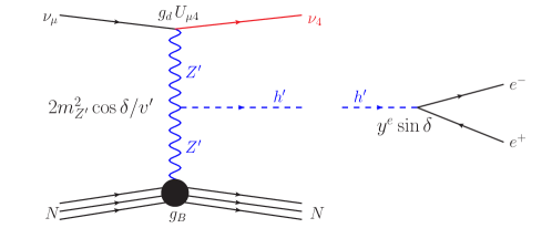
Figure 1: Feynman diagram of the scattering process in our model which leads to the excess in MB. Note that $H$ also contributes via the same diagram.

To compute the total differential cross section, we consider both the incoherent and coherent contributions in the production of $h^{\prime}$, as shown in Fig. 1. The total differential cross section, for the target in MB, ${\it i.e.}$, CH₂, is given by

$$\left(\dfrac{d\sigma}{dE_{h^{\prime}}}\right)_{{\rm CH_{2}}}=\underbrace{14\times\left(\dfrac{d\sigma}{dE_{h^{\prime}}}\right)}_{\textrm{\footnotesize{{incoherent}}}}+\underbrace{144\times exp(2b(k^{\prime}-k)^{2})\left(\dfrac{d\sigma}{dE_{h^{\prime}}}\right)}_{\textrm{\footnotesize{{coherent}}}}.$$ (34)

For the incoherent process, we have multiplied the single nucleon cross section by the total number of the nucleons present in CH₂ i.e., 14. In the coherent process the entire carbon nucleus (C¹²) contributes in the process and the contribution is large when the momentum transfer is small, i.e. $q^{2}=(k^{\prime}-k)^{2}\sim 0$. As $q^{2}$ increases, the coherent contributions are reduced significantly. This is implemented by the form factor $exp(2b(k^{\prime}-k)^{2})$ Hill (2010), where $b$ is a numerical parameter, which for C¹², has been chosen to be $25$ GeV^-2 Freedman (1974); Hill (2010).

We have used Eq. (34) to calculate the total number of $h^{\prime}$ produced in the final state. Once $h^{\prime}$ is produced, it decays promptly to an $e^{+}e^{-}$ pair, its lifetime being decided by its coupling to electrons. Neglecting the mass of the electron, the lifetime of $h^{\prime}$ is given by

$$\tau_{h^{\prime}}=\dfrac{8\pi}{(y^{h^{\prime}}_{e})^{2}\,m_{h^{\prime}}}.$$ (35)

For our benchmark parameter values, the lifetime of $h^{\prime}$ is $3.5\times 10^{-13}$ seconds. We note that MB is not able to distinguish an $e^{+}e^{-}$ pair from a single electron Jordan et al. (2019); Karagiorgi (2010) if $m_{\rm track}<30$ MeV, where

$$m_{\rm track}\equiv\sqrt{2E_{1}E_{2}(1-\cos\theta_{12})}.$$ (36)

Here $E_{1}$ and $E_{2}$ are the track energies and $\theta_{12}$ is the angle between two tracks. Since we have chosen the mass of $h^{\prime}$ to be 23 MeV, the $m_{\rm track}$ produced by $h^{\prime}$ decay is always less than 30 MeV. Hence, the decay of $h^{\prime}$ to an $e^{+}e^{-}$ pair mimics the single electron charged current quasi-elastic (CCQE) signal in the detector. We note that $H$ can also contribute to the MB signal, since it can be produced in the final state and subsequently decay promptly to an $e^{+}e^{-}$ pair. If the opening angle of the two electrons is less than $8^{\circ}$ or one of electrons has energy less than $30$ MeV, it would add to the signal. We find that only a fraction $(\sim 10-15\%)$ of the total number of the $H$ produced satisfy these criteria. Further suppression are provided by kinematics, since its mass is higher than that of $h^{\prime}$, and by $\sin^{2}\delta$. Hence, the contribution of $H$ to the MB events is small. Additionally, we have checked that the production of two $h^{\prime}$s, two $H$s or $h^{\prime}H$ via the quartic couplings to $Z^{\prime}$ is suppressed compared to single $h^{\prime}$ production in the final state.

Our results are presented in the next section.

IV Results

In this section we present the results of our numerical calculations, using the cross section for the process and the model described in Section III.

IV.1 Results for MiniBooNE and implications for LSND and KARMEN

Fig. 2 shows, in each of the 4 panels, the data points, SM backgrounds and the prediction of our model (blue solid line) in each bin. Also shown (black dashed line) is the oscillation best fit. The left panel plots show the distribution of the measured visible energy, E_vis, plotted against the events for neutrinos (top) and anti-neutrinos (bottom). For our model, E_vis corresponds to $E_{h^{\prime}}$. The right panels show the corresponding angular distributions for the emitted light. The benchmark parameter values used to obtain the fit from our model are shown in Table 1. The plots have been prepared using fluxes, efficiencies POT exposures and other relevant information from Aguilar-Arevalo et al. (2018b, 2020) and references therein. We see that very good fits to the data are obtained both for energy and angular distributions. (The data points show only statistical uncertainties.). We have assumed a $15\%$ systematic uncertainty for our calculations. These errors are represented by the blue bands in the figures.

$m_{\nu_{4}}$ (MeV)	$m_{Z^{\prime}}$ (MeV)	$m_{h^{\prime}}$ (MeV)	$m_{H}$ (MeV)	$|U_{\mu 4}|^{2}$	$g_{B}$	$g_{d}$	$\sin\delta$	$y_{e(\mu)}^{h^{\prime}}\!=\!y^{e(\mu)}\sin\delta$	$y_{e(\mu)}^{H}\!=\!y^{e(\mu)}\cos\delta$	$|y^{e\tau}y^{\tau e}|$
50	$800$	$23$	$106$	$2.6\!\times\!10^{-5}$	$3\!\times\!10^{-4}$	$2.85$	0.28	$0.45(1.8)\!\times\!10^{-4}$	$1.5(6.0)\!\times\!10^{-4}$	$5.6\!\times\!10^{-7}$

Table 1: Benchmark parameter values used for event generation in MB and for calculating the muon and electron $g-2$.

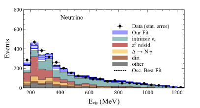
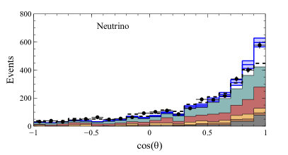
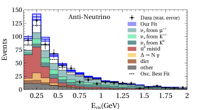
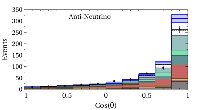
Figure 2: The MB electron-like events (backgrounds and signal) from Aguilar-Arevalo et al. (2018b, 2020), versus the visible energy E_vis and versus the cosine of the emitted angle of the light, for neutrino (top) and anti-neutrino (bottom) runs. Data points show statistical errors, whereas the blue band shows (estimated) systematic errors. The blue solid line is the prediction of our model. The parameter values used in calculating it are shown in Table 1.

As mentioned earlier, the LSND observations measure the visible energy from the Cerenkov and scintillation light of an assumed electron-like event, as well as the $2.2$ MeV photon resulting from coincident neutron capture on hydrogen. In our model, this corresponds to the scattering diagrams in Fig. 1 where the target is a neutron in the Carbon nucleus. Unlike the case of MB above, where both coherent and incoherent processes contribute to the total cross section, the LSND cross section we have used includes only an incoherent contribution. Using the same benchmark parameters as were used to generate the MB results, as well as all pertinent information on fluxes, efficiencies, POT etc from Athanassopoulos et al. (1995); Athanassopoulos et al. (1996a, b, 1998); Aguilar-Arevalo et al. (2001), we find a very small excess ($1-2$ events, from the DIF flux only), compared to the much larger observed excess reported by LSND Aguilar-Arevalo et al. (2001). We note that our calculations do not include effects arising from final state interactions or other considerations like nuclear screening or multiple scattering inside the nucleus, which could play a role at the LSND energies Betancourt et al. (2018). The KARMEN experiment similarly employed a mineral oil detection medium, but was less than a third of the size of LSND. It did not have a significant DIF flux, but had similar incoming proton energy and efficiencies. Unlike LSND, it saw no evidence of an excess. A simple scaling estimate using our LSND result gives $\sim 0$ events in KARMEN using our model, which is consistent with their null result.

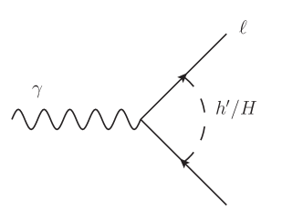
Figure 3: One-loop contribution to lepton anomalous magnetic moments from the neutral scalars $h^{\prime}$ and $H$.

IV.2 Muon anomalous magnetic moment

The one-loop contribution of a scalar $\phi$ (as shown in Fig. 3) to the muon anomalous magnetic dipole moment is given by Jackiw and Weinberg (1972); Leveille (1978)

$$\Delta a^{\phi}_{\mu}=\frac{(y^{\phi}_{\mu})^{2}}{8\pi^{2}}\int_{0}^{1}dx\frac{(1-x)^{2}(1+x)}{(1-x)^{2}+x\,r_{\phi}^{2}},$$ (37)

where $r_{\phi}=m_{\phi}/m_{\mu}$, and $\phi=h^{\prime},H$. $y^{\phi}_{\mu}$ is the coupling strength of the scalar $\phi$ with the muon pair, which is defined in Eq. (30).

In our scenario, both $h^{\prime}$ and $H$ have comparable contributions to the muon anomalous magnetic moment given that they have light masses $\leq 1$ GeV Liu et al. (2020, 2019). In Fig. 4, we show the relative contributions of $h^{\prime}$ and $H$ to $\Delta{a_{\mu}}$ as a function of the scalar mixing angle $\delta$. The blue dashed and red dotted lines correspond to the muon anomalous magnetic moment contributions of $H$ and $h^{\prime}$ ($\Delta a_{\mu}^{H}$ and $\Delta a_{\mu}^{h^{\prime}}$), respectively, while the green solid line refers to their sum ($\Delta a_{\mu}^{H}+\Delta a_{\mu}^{h^{\prime}}$). In addition, the horizontal yellow band indicates the $3.7\sigma$ muon $g-2$ discrepancy: $\Delta a_{\mu}=(2.79\pm 0.76)\times 10^{-9}$ Aoyama et al. (2020) and the black star denotes our benchmark in Table 1. We note that in this figure $m_{h^{\prime}}$, $m_{H}$ are fixed to fit the MB measurements, as discussed in the previous section. We see that both $h^{\prime}$ and $H$ have reasonable and comparable contributions to the total muon anomalous magnetic moment $\Delta a_{\mu}$ and their ratio $\Delta a_{\mu}^{h^{\prime}}/\Delta a_{\mu}^{H}\sim\tan^{2}\delta$. Although in our scenario are fixed $m_{h^{\prime}}$ and $m_{H}$ to fit the MB measurements, in a more general situation $y^{\mu}$ and the angle $\delta$ are still free parameters and one can fix them to fit the central value for $\Delta a_{\mu}$.

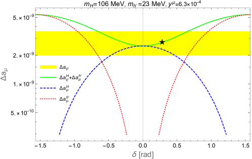
Figure 4: Muon anomalous magnetic moment versus the scalar mixing angle $\delta$, along with our benchmark in Table 1 denoted by the black star.

For a suitably selected combination of $y^{\mu}$ and $\delta$ ($y^{\mu}=6.3\times 10^{-4}$ and $\sin\delta=0.28$), our benchmark (denoted by the black star) is situated in the experimental allowed region (yellow band), close to the central value for $\Delta a_{\mu}$ ($=2.74\times 10^{-9}$). For our benchmark, it is clearly seen that while the total muon anomulous magnetic moment $\Delta a_{\mu}$ is dominated by the $H$ contribution $\Delta a_{\mu}^{H}$ (blue dashed line), the $h^{\prime}$ contribution (red dotted line) is $18\%$ of $\Delta a_{\mu}$, which is not negligible. The constraints on $y^{\phi}_{\mu}~{}(\phi=h^{\prime},H)$ are shown in Fig. 9. We see that both $y^{h^{\prime}}_{\mu}$ and $y^{H}_{\mu}$ sit in the experimentally allowed region of the current constraint of BaBar Lees et al. (2014) and the future sensitivity of Belle-II Batell et al. (2018).

IV.3 Electron anomalous magnetic moment

In this sub-section, we consider the one-loop contribution of a light scalar $\phi$ ($h^{\prime},H$ in our model) to the electron anomalous magnetic moment which is given by Jackiw and Weinberg (1972); Leveille (1978)

$$\Delta a^{\phi}_{e}=\sum_{\ell=e,\mu,\tau}\frac{y^{\phi}_{e\ell}\,y^{\phi}_{\ell e}}{8\pi^{2}}\int_{0}^{1}dx\frac{(1-x)^{2}(r_{\ell}+x)}{(1-x)^{2}+x\,r_{\phi}^{2}+(1-x)(r_{\ell}^{2}-1)},$$ (38)

where $r_{X}=m_{X}/m_{e}$ and $y^{\phi}_{ee}=y^{\phi}_{e}$ is the coupling strength of the scalar $\phi$ with the electron pair, as defined in Eq. (30). To evade the BR($\mu\to e\gamma$) and BR($\tau\to\mu\gamma$) experimental upper bounds Baldini et al. (2016); Aubert et al. (2010) and explain the electron $g-2$ anomaly, hereafter, we have chosen $y_{\mu e(e\mu)}^{\phi}$ and $y_{\mu\tau(\tau\mu)}^{\phi}$ to be sufficiently tiny and the product $y^{\phi}_{\tau e}y^{\phi}_{e\tau}$ is negative. Overall, $\Delta{a_{e}}$ gets a positive contribution due to the non-vanishing Yukawa couplings $y^{\phi}_{e}$ which are fixed to fit the MB measurements, as discussed in section IV.1. Also, it gets a negative contribution from $\tau$ inside the loop, since the product $y^{\phi}_{\tau e}y^{\phi}_{e\tau}$ is negative and is essentially a free parameter in our scenario. Thus, one can choose the absolute value of this product to fit the central value of $\Delta a_{e}$. Note that $y^{h^{\prime}}_{\tau e(e\tau)}=y^{\tau e(e\tau)}\sin\delta$ and $y^{H}_{\tau e(e\tau)}=y^{\tau e(e\tau)}\cos\delta$.

In our scenario, as mentioned earlier, $h^{\prime}$ and $H$ have light masses and consequently both contribute to the electron $g-2$ anomaly, $\Delta a_{e}$. In Fig. 5, we show the relative contributions of $h^{\prime}$ and $H$ to $\Delta{a_{e}}$ versus the absolute product $|y^{e\tau}y^{\tau e}|$. The blue dashed and red dotted lines correspond to the electron anomalous magnetic moment contributions of $H$ and $h^{\prime}$ ($\Delta a_{e}^{H}$ and $\Delta a_{e}^{h^{\prime}}$), respectively, while the green solid line refers to their sum ($\Delta a_{e}^{H}+\Delta a_{e}^{h^{\prime}}$). In addition, the horizontal yellow band indicates the $2.4\sigma$ discrepancy between the experimental measurement and theoretical prediction: $\Delta a_{e}=(-8.7\pm 3.6)\times 10^{-13}$ Parker et al. (2018). We see that both $h^{\prime}$ and $H$ have approximately the same positive contribution ($\simeq 10^{-13}$) to the total electron anomalous magnetic moment $\Delta a_{e}$ at $|y^{e\tau}y^{\tau e}|=0$, which is coming from $e$ inside the loop (electron contribution). Additionally, since the contribution of $\tau$ inside the loop (tau contribution) which owes its sign to the product $y^{\phi}_{\tau e}y^{\phi}_{e\tau}$ is negative, $\Delta a_{e}$ gets a negative contribution overall. This originates mainly from the $H$ contribution ($\Delta a_{e}^{H}$), as it is clearly seen from Fig. 5. In this figure, the other relevant parameters have the benchmark values shown in Table 1. It is clear that for $|y^{e\tau}y^{\tau e}|\simeq 5.6\times 10^{-7}$, our benchmark sits near the central value for $\Delta a_{e}$ ($=-8.7\times 10^{-13}$).

Figure 5: Electron anomalous magnetic moment as a function of the absolute value of $y^{e\tau}y^{\tau e}$.

V Discussion on Constraints

This section is devoted to a discussion of constraints that the proposed scenario must satisfy, and related issues as well as future tests of the various elements of our proposal. Subsection A focuses on bounds related to the additional $U(1)$ and its gauge boson and couplings, while Subsection B discusses constraints related to the scalar sector extension. We have, for the most part, restricted our discussion to the regions of parameter space relevant to our scenario.

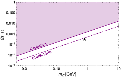
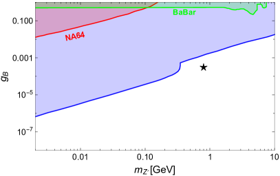
Figure 6: Constraints on $m_{Z^{\prime}}$ and $g_{B-3L_{\tau}}$ from oscillation experiments, denoted by the solid line and shaded region above it, along with projected sensitivities of T2K and DUNE (left panel, adapted from Han et al. (2019)) and on $m_{Z^{\prime}}$ and $g_{B}$ from NA64 Banerjee et al. (2018) and BaBar Lees et al. (2017), along with theoretical bounds from (see text) Dror et al. (2017a, b) (right panel, adapted from Ilten et al. (2018)) along with our benchmark in Table 1 denoted by the black star.

V.1 The $U(1)$ extension

Constraints on $m_{Z^{\prime}}$ and $g_{B-3L_{\tau}}$: Strong constraints on this coupling and the associated $Z^{\prime}$ mass arise from oscillation experiments as well as various decay searches Tulin (2014); Farzan and Heeck (2016); Heeck et al. (2019); Han et al. (2019). Fig. 6 (left panel) shows these bounds, along with our benchmark point. We note that there is a significant difference between the bounds on the coupling coming from Han et al. (2019) and Heeck et al. (2019). The reason lies in the choice, respectively, of the LMA and LMA $+$ LMA-D and KamLAND solutions made by them. For more details the reader is referred to Esteban et al. (2018). Our benchmark point is compatible with both bounds, comfortably with Han et al. (2019), but only marginally so with Heeck et al. (2019). Future tests of these parameter values would be possible via oscillation measurements at DUNE Acciarri et al. (2015) and T2HK Abe et al. (2018), as discussed in Han et al. (2019). Other experiments sensitive to $\tau$ interactions, like DONuT Kodama et al. (2008) and the future emulsion detectors SHiP Anelli et al. (2015), FASER$\nu$ Abreu et al. (2020a, b) and SND@LHC Ahdida et al. (2020) could provide additional constraints on the parameter space for $m_{Z^{\prime}}$ and $g_{B-3L_{\tau}}$ Kling (2020).

Constraints on $m_{Z^{\prime}}$ and $g_{B}$: The gauging of baryon number via a light boson associated with a $U(1)_{B}$ symmetry, which primarily interacts with quarks is subject to a number of constraints on its mass $m_{Z^{\prime}}$ and the gauge coupling $g_{B}$ Ilten et al. (2018). Assuming that the primary modes of decay are invisible, the strongest of these come from theoretically computed bounds arising from anomaly cancellation by heavy fermions, which lead to enhanced interaction rates for processes involving the longitudinal mode of the $Z^{\prime}$ Dror et al. (2017a, b). In addition, constraints from searches by NA64 Banerjee et al. (2018) and BaBar Lees et al. (2017) for a light vector decaying to invisible become relevant. We show these in Fig. 6 (right panel), along with our benchmark values.

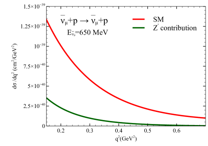
Figure 7: The SM NC quasi-elastic anti-neutrino-proton cross section, compared to the contribution obtained from our model with the $Z^{\prime}$ due to its couplings to baryons and to $\nu_{d}$. The parameter values used in calculating the $Z^{\prime}$ contributions are the same as those used for our MB result, and are given in Table 1.

Contributions to NC $\nu$-nucleon scattering at both low and high energies: At low energies, an important constraint arises from NC quasi-elastic neutrino-nucleon scattering, to which the new $Z^{\prime}$ would contribute via an amplitude proportional to $g_{d}\,g_{B}\,U_{\mu 4}$. MB has measured this cross section in the relevant range Perevalov and Tayloe (2009). Fig. 7 shows the SM differential cross section for muon anti-neutrino scattering and compares it to the cross section from our model. We see that the contribution from the latter stays safely below the SM anti-neutrino cross section, which, of course, is lower than that for neutrinos and thus provides a more conservative basis for comparison. We note that our process with the $Z^{\prime}$ mediator does not distinguish between neutrino and anti-neutrino scattering, unlike the SM case. It also adds $10-25\%$ to the SM cross section, over the range shown. Interestingly, MB NC measurements have been fitted with an axial mass $M_{A}$ which is significantly higher than the value from the global average value of this parameter, indicating that the measured cross section is higher than expected, with one possible conclusion being that it is receiving contributions from new physics.

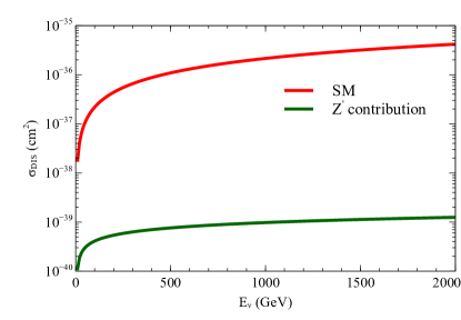
Figure 8: The SM NC DIS cross section, compared to that obtained from our model. The parameter values used in calculating the $Z^{\prime}$ contribution are given in Table 1.

IceCube and DeepCore are a possible laboratory for new particles which are produced via neutrino nucleon scattering Coloma et al. (2017); Coloma (2019). Fig. 8 shows our check for contributions of the model to deep inelastic scattering (DIS), comparing it to the SM total NC cross section for ${\nu_{\mu}}$-nucleon scattering. The $Z^{\prime}$ contributions are more than three orders of magnitude lower. We note that the DeepCore and IceCube detectors would be sensitive to the new particles and the interaction in our model in two ways: $a)$ by a possibly measurable increase in the neutrino nucleon NC event rate, and $b)$ via the decay of $h^{\prime}$ into an $e^{+}e^{-}$ pair if, after its production in a NC event mediated by $Z^{\prime}$, it travels a distance long enough to signal a double bang event (about 10 m in DeepCore, and $\sim$ a few hundred m in IceCube). The lifetime of the $h^{\prime}$ in our scenario is $c\tau\sim 10^{-4}$ m. The distances travelled even at very high energies are much smaller than the resolution necessary to signal a double bang event. In addition, as Fig. 8 shows, the high energy NC cross section stays several orders of magnitude below the SM cross section. We note that similar to the low-energy case above, the $Z^{\prime}$ contribution has been calculated taking into account the enhancement it receives due to $g_{d}\,U_{\mu 4}$ at the neutrino vertex.

Constraints on $m_{\nu 4}$, $|U_{\mu 4}|$ and $|U_{e4}|$: The mass of the dark neutrino in our model has a wider possible range than that in scenarios where it is required to decay inside the MB detector Gninenko (2011); Bertuzzo et al. (2018); Ballett et al. (2019b) to obtain the electron-like signal. Its main role here is that of a portal connecting the SM neutrinos via mixing to the $Z^{\prime}$. Nonetheless, heavy sterile neutrino masses and mixings are tightly constrained by a number of experiments, as well as astrophysics and cosmology, and these bounds are discussed and summarized in Bolton et al. (2020); Atre et al. (2009); McKeen and Pospelov (2010); Duk et al. (2012); Drewes and Garbrecht (2017); de Gouvêa and Kobach (2016); Argüelles et al. (2019c); Bryman and Shrock (2019a, b). We assume that the $\nu_{d}$ does not constitute an appreciable fraction of DM in the universe, and has dominantly invisible decay modes. Our benchmark value for its mass is $\sim 50$ MeV, and this along with the mixings we assume are in conformity with the existing bounds.

Constraints from NOMAD: The NOMAD experiment carried out a search for neutrino induced single photon events at high energies, $E_{\nu}\sim 25$ GeV Kullenberg et al. (2012). It obtained an upper limit of $4.0\times 10^{-4}$ single photon events for every ${\nu_{\mu}}$ induced charged-current event. Clearly, extrapolating our calculations to NOMAD energies would be invalid, given that the calculational procedures we use to obtain the pair production contributions do not apply there. NOMAD used coherent pion kinematics with one photon to arrive at their bound. We then examine the ratio of the cross section for our process, including coherent effects, to the charged current total inclusive incoherent muon production cross section measured by NOMAD at $E_{\nu}\sim 25$ GeV, and obtain a ratio below the upper bound given by NOMAD.

Constraints from CHARM II and MINERVA: We find that in our model, the $Z^{\prime}$ does contribute to the neutrino electron scattering cross section at these detectors to the extent of about $\sim 14\%$, leading to a very mild tension with their observations when flux and other uncertainties are accounted for.

Constraints from CE${\nu}$NS: Any additional $U(1)$ with a vector $Z^{\prime}$ mediator that couples to neutrinos and baryons could conceivably receive large contributions from coherent elastic neutrino-nucleon scattering (CE${\nu}$NS) Freedman (1974); Kopeliovich and Frankfurt (1974), since it would receive an enhancement proportional to the square of the number of nucleons. In our scenario, in spite of the choice of gauge groups being $U(1)_{B-3L\tau}$ or $U(1)_{B}$, the $Z^{\prime}$ does effectively couple to muon neutrinos (Fig. 1). The amplitude for this process receives an added enhancement from the fact that the effective active neutrino-$Z^{\prime}$ coupling is $g_{d}\,U_{\mu 4}$, which can be significantly larger than $g_{B}$.

The COHERENT Collaboration Akimov et al. (2017) has recently observed CE${\nu}$NS, for neutrinos in the energy range of $16-53$ MeV, and concurrently set stringent bounds on the parameters $g_{B}$ and $m_{Z^{\prime}}$. The values of $g_{B}$ and $m_{Z^{\prime}}$ chosen by us respect these constraints, but the coupling for the amplitude of the enhanced process, $g_{B}\,g_{d}\,U_{\mu 4}$ does not. However, the neutrino beam energies in COHERENT are below the kinematic range required for the process in Fig. 1, since besides nuclear/nucleon recoil, a heavy neutrino of mass $\sim 50$ MeV must be produced in the final state. Thus the event rate in COHERENT remains unaffected by our scenario.

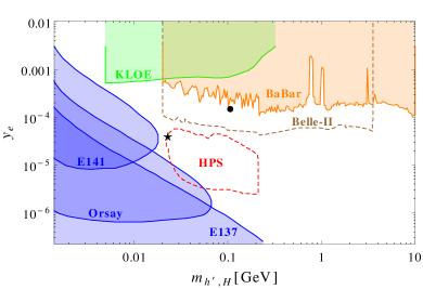
Figure 9: Relevant constraints to our scenario, where the color shaded regions with solid boundary indicate to the excluded regions by current experiments, and the unshaded regions with dashed boundaries are future projections (see text for details).

V.2 The extended scalar sector

Constraints on $y_{e}$ and $m_{h^{\prime}}$ from dark photon searches: A dark photon search looks for its decay to lepton pair. These bounds can be translated Alves and Weiner (2018); Knapen et al. (2017) to constraints on a light scalar which couples to leptons. We show these translated constraints relevant to our scenario from KLOE Anastasi et al. (2015), BaBar Lees et al. (2014) and the projected future sensitivity from Belle-II in Fig. 9 (left panel) Batell et al. (2018).

Constraints on $y_{e}$ and $m_{h^{\prime}}$ from electron beam dump experiments: A light scalar with couplings to electrons could be searched for Liu et al. (2016); Batell et al. (2017) in beam dump experiments via its decay to an $e^{+}e^{-}$ pair or photons. Relevant to the mass range under consideration here are the experiments E137 Bjorken et al. (1988), E141 Riordan et al. (1987) and ORSAY Davier and Nguyen Ngoc (1989). The forbidden regions are shown in Fig. 9 (left panel). In the future, the HPS fixed target experiment Battaglieri et al. (2015) which will scatter electrons on tungsten, will be able to constrain the displaced decays of a light scalar. Its projected sensitivity is also shown in this figure.

Constraints from ND280: As discussed in Brdar et al. (2020), the T2K near-detector, ND280, is in a position to provide bounds on new physics related to the MB LEE. Relevant to our work here, the specific decay $h^{\prime}\rightarrow e^{+}e^{-}$ could be observable in the Ar TPC associated with this detector. In our model, however, this decay is prompt, hence the Ar gas must act as both target and detection medium if this is to be observed. Since the target mass is only 16 kg, however, the number of events is unobservably small in our case.

Future tests of the muon and the electron $g-2$: The E989 experiment Grange et al. (2015) at Fermilab is soon likely to announce results of measurements of the muon $g-2$ which will have significantly higher precision than current measurements. This will be complemented by measurements of this quantity at comparable precision by an experiment at J-PARC and the E34 Collaboration Abe et al. (2019). An important supplementary effort will be the measurement of the hadronic contributions to the muon magnetic moment by the MUonE experiment Abbiendi et al. (2017) at CERN, which will determine them at uncertainties below those in present theoretical calculations. Finally, continuing and improved measurements of the fine structure constant are likely to determine the future significance of the discrepancy in the electron $g-2$.

Constraints on $y_{\mu}$ and $m_{H}$ from colliders: BaBar has provided constraints Batell et al. (2017, 2018) on these parameters via their search for $e^{+}e^{-}\rightarrow\mu^{+}\mu^{-}\phi$, where $\phi$ is a generic light scalar. Also shown in Fig. 9 (right panel) is the future projection for Belle-II Batell et al. (2018). Our benchmark points, as shown, are below these bounds.

Constraints on $y_{\tau}$ and $m_{H}$ from BaBar: Very recently, BaBar has provided strong constraints Lees et al. (2020) on the parameter $\xi$, which is the ratio of the effective coupling ($y_{e,\mu,\tau}$ in our model) of a light scalar to a fermion compared to its SM Yukawa coupling $(m_{f}/v)$. BaBar looks for narrow width decays of a leptophilic scalar $\phi$, produced radiatively from $\tau$-lepton via $e^{+}e^{-}\rightarrow\tau^{+}\tau^{-}\phi$, followed by $\phi\rightarrow e^{+}e^{-}$. In our case, noting that $y_{e,\mu,\tau}$ are all independent, this translates to a bound on $y_{\tau}$ and $m_{H}$. For our mass range for $H$, of $100-150$ MeV, this implies that $y_{\tau}$ remain below $\approx 3.5\times 10^{-3}$. In our scenario, $y_{\tau}$, is independent and essentially free, and can be kept small. We also note that the independence of $y_{\mu}$ from $y_{\tau}$ in our scenario ensures that the bound on $y_{\tau}$ from BaBar does not automatically translate into a bound on $y_{\mu}$, unlike the case where $\xi$ is the same for all leptonic generations.

Constraints from $\tau\to e\gamma$ : In our calculation for $\Delta a_{e}$, the BR($\tau\to e\gamma$) has a non-zero value due to the non-vanishing Yukawa couplings of the $\phi$-$e$-$\tau$ interactions, $y^{\phi}_{\tau e(e\tau)}$. We thus calculated this BR($\tau\to e\gamma$) Lavoura (2003) mediated by the light scalars $h^{\prime}$ and $H$ using $|y^{e\tau}y^{\tau e}|\simeq 5.6\times 10^{-7}$. We find that this yields a total BR$(\tau\to e\gamma)\simeq 5.4\times 10^{-10}$. We note that this is very small compared with the experimental upper bound, BR$(\tau\to e\gamma)<1.1\times 10^{-7}$ Aubert et al. (2010), and hence is not a concern.

Constraints from Higgs physics:. We note that in the model considered here, the $h$ is almost identical to the SM Higgs, with negligible mixings to the other neutral scalars ($h^{\prime}$ and $H$). This makes the constraints from Higgs observations not a matter of immediate concern.

Stability of the scalar potential: We have examined the behaviour of the potential as the fields tend to infinity, in order to ensure it is stable. Our benchmark parameters satisfy the vacuum stability conditions. The details are provided in the Appendix B.

Collider constraints on the heavy charged CP-even scalars $H^{\pm}$: Drell-Yan processes at both LEP and the LHC can produce pairs of the $H^{\pm}$, which can subsequently decay to a neutrino and a lepton each. Bounds set on supersymmetric particles Sirunyan et al. (2018); Aad et al. (2014); Sirunyan et al. (2019) which would mimic these final states can be translated to bounds on $H^{\pm}$, as discussed in Babu et al. (2020); Jana et al. (2020). These lead to a lower bound on the charged scalar mass of $m_{H^{\pm}}>110$ GeV.

Electro-weak precision constraints on the heavy charged CP-even scalars $H^{\pm}$ and pseudoscalar $A$: The oblique parameters $S,T$ and $U$ are a measure of the effects new particles can have on gauge boson self energies. The effects of scalars in an expanded Higgs sector on these parameters have been discussed in Funk et al. (2012); Grimus et al. (2008a, b). For models in the alignment limit, bounds using the $T$ parameter are particularly significant in constraining the plane of mass differences between $a)$ the SM-like Higgs and the charged $H^{\pm}$, and $b)$ the $H^{\pm}$ and the pseudoscalar Jana et al. (2020); Babu and Jana (2019). Essentially, one finds that either the masses of the pair in $a)$ or that in $b)$ need to be close to each other, while the other mass difference can be large, ${\it e.g.}\sim$ a few hundred GeV. In our scenario, if the dominant contribution to $\Delta a_{\mu}$ is to originate from an $H$ with a mass below $200$ MeV, one is led to the mass hierarchy $m_{A}\sim m_{H^{\pm}}$ $\gg m_{H}$.

VI Summary and concluding remarks

Among several anomalous signals at low energy experiments, the MB LEE and the discrepancy in the measured value of the anomalous magnetic moment of the muon stand out, due to their statistical significance, the duration over which they have been present and the scrutiny and interest they have generated. Our effort in this paper takes the viewpoint that these anomalies are due to interlinked underlying new physics involving a new $U(1)$ connecting the SM and the dark sector.

Pursuant to this, starting with the MB LEE, we find that a light $Z^{\prime}$ vector portal associated with $U(1)_{B-3L_{\tau}}$, which is anomaly-free, or a $U(1)_{B}$ extension of the SM, combined with a second Higgs doublet allows a very good fit to the excess. The $Z^{\prime}$ obtains its mass from a dark sector singlet scalar, and is coupled to a dark neutrino. The Higgs sector thus comprises of three CP-even scalars, $h$, which is predominantly SM Higgs-like, and $h^{\prime}$ and $H$ which are light compared to $h$ and the charged Higgses of the model. $h^{\prime},H$ are coupled both to the dark sector and to SM fermions via mixing. In MB, the $h^{\prime}(H)$ is produced via the $Z^{\prime}$-$h^{\prime}(H)$-$Z^{\prime}$ coupling and decays primarily to an $e^{+}e^{-}$ pair. Both $h^{\prime}$ and $H$ contribute to both the MB LEE and the muon and electron $g-2$, but for our choice of benchmarks, the $h^{\prime}(H)$ contributes dominantly to the MB LEE (the muon and electron $g-2$).

Our work underscores the role light scalars may play in understanding low energy anomalies that persist and survive further tests, and the possibility that a light $Z^{\prime}$ may provide an important portal to the dark sector. This $Z^{\prime}$ need not be unique as long as it couples in a flavor universal way to quarks. The couplings to leptons are constrained to be very small, however, especially for the first two generations. Overall, we provide a template for a model with an additional $U(1)$ that agrees very well with MB data while staying in conformity with all known constraints.

We note that a singlet scalar mass-mixed with the SM Higgs along with the $Z^{\prime}$, could, in principle have provided an economical solution for the MB LEE. However, the fermionic couplings of such a scalar are constrained to be very tiny and cannot be used to generate the MB excess. This motivates the need for a second Higgs doublet mixed with the dark sector. We find that when incorporated, the interplay of the scalars via mixing allows us to understand both the MB signal and the observed anomalous value of the muon magnetic moment in a manner that satisfies existing constraints.

Appendices

Appendix A Diagonalization of CP-even Higgs mass matrix

In the basis $\left(H_{1}^{0},H_{2}^{0},H_{3}^{0}\right)$, the mass matrix of the neutral CP-even Higgses is given by

$$m^{2}_{\cal H}=\left(\begin{array}[]{ccc}\lambda_{1}v^{2}&\lambda_{6}v^{2}&\lambda^{\prime}_{3}vv^{\prime}\\ \lambda_{6}v^{2}&\bar{m}_{H}^{2}&\lambda^{\prime}_{5}vv^{\prime}\\ \lambda^{\prime}_{3}vv^{\prime}&\lambda^{\prime}_{5}vv^{\prime}&2\lambda^{\prime}_{2}v^{\prime 2}\end{array}\right).$$ (39)

Now if $\lambda_{6}\simeq 0\simeq\lambda^{\prime}_{3}$, then we get the alignment limit i.e. one of the CP-even Higgs mass eigenstates aligns with the vev direction of the scalar field. In the alignment limit, the mass matrix becomes

$$m^{2}_{\cal H}\simeq\left(\begin{array}[]{ccc}\lambda_{1}v^{2}&0&0\\ 0&\bar{m}_{H}^{2}&\lambda^{\prime}_{5}vv^{\prime}\\ 0&\lambda^{\prime}_{5}vv^{\prime}&2\lambda^{\prime}_{2}v^{\prime 2}\end{array}\right).$$ (40)

Now,

$${Z^{\cal H}}m^{2}_{\cal H}(Z^{\cal H})^{T} = ({\cal M}^{2})^{\rm diag}={\rm diag}\{m_{h}^{2},m_{H}^{2},m_{h^{\prime}}^{2}\},$$ (41)

where

$${Z^{\cal H}}=\left(\begin{array}[]{ccc}1&0&0\\ 0&\cos\delta&-\sin\delta\\ 0&\sin\delta&\cos\delta\\ \end{array}\right),~{}~{}{\rm with}~{}~{}\tan{2\delta}=\frac{-2\lambda^{\prime}_{5}vv^{\prime}}{\bar{m}_{H}^{2}-2\lambda^{\prime}_{2}v^{\prime 2}}.$$ (42)

The eigenvalues of the mass matrix are

$$m^{2}_{h,H,h^{\prime}}\simeq\left\{\lambda_{1}v^{2},\frac{1}{2}\left(\bar{m}_{H}^{2}+2\lambda^{\prime}_{2}v^{\prime 2}\pm\sqrt{(\bar{m}_{H}^{2}-2\lambda^{\prime}_{2}v^{\prime 2})^{2}+4(\lambda^{\prime}_{5}vv^{\prime})^{2}}\right)\right\}.$$ (43)

If we choose $\bar{m}_{H}^{2}=(102~{}\rm{MeV})^{2}$, $\lambda^{\prime}_{5}vv^{\prime}=-(53.8~{}\rm{MeV})^{2}$ and $2\lambda^{\prime}_{2}v^{\prime 2}=(37~{}\rm{MeV})^{2}$, we get $m_{H}=106$ MeV, $m_{h^{\prime}}=23$ MeV and $\sin\delta=0.28$, which fit our benchmark in Table 1.

Appendix B Vacuum Stability

For a stable vacuum, the potential should be bounded from below as the field strength approaches to infinity from any directions. In this limit, only the quartic part of the potential is relevant. In the alignment limit ($\lambda_{6}\simeq 0\simeq\lambda^{\prime}_{3}$) and for simplicity we consider $\lambda_{7}=0=\lambda^{\prime}_{4}$. With those considerations, the quartic part of the potential becomes

$$V_{4} = \frac{\lambda_{1}}{2}(\phi_{h}^{\dagger}\phi_{h})(\phi_{h}^{\dagger}\phi_{h})+\dfrac{\lambda_{2}}{2}(\phi_{H}^{\dagger}\phi_{H})(\phi_{H}^{\dagger}\phi_{H})+\lambda_{3}(\phi_{h}^{\dagger}\phi_{h})(\phi_{H}^{\dagger}\phi_{H})+\lambda_{4}(\phi_{h}^{\dagger}\phi_{H})(\phi_{H}^{\dagger}\phi_{h})$$ (44)

$$+ \frac{\lambda_{5}}{2}((\phi_{h}^{\dagger}\phi_{H})^{2}+(\phi_{H}^{\dagger}\phi_{h})^{2})+\lambda^{\prime}_{2}(\phi_{h^{\prime}}^{\ast}\phi_{h^{\prime}})^{2}+\lambda^{\prime}_{5}(\phi_{h^{\prime}}^{\ast}\phi_{h^{\prime}})(\phi_{h}^{\dagger}\phi_{H}+\phi_{H}^{\dagger}\phi_{h}).$$

We can parameterize the fields as El Kaffas et al. (2007)

$$|\phi_{h}|=rc_{\vartheta}s_{\varphi},~{}~{}~{}~{}~{}|\phi_{H}|=rs_{\vartheta}s_{\varphi},~{}~{}~{}~{}~{}|\phi_{h^{\prime}}|=rc_{\varphi},~{}~{}~{}~{}~{}\phi_{h}^{\dagger}\phi_{H}=|\phi_{h}||\phi_{H}|\,\rho\,e^{i\gamma},$$ (45)

where $s_{x}\equiv\sin x$, $c_{x}\equiv\cos x$, $r\geq 0,\,\,\vartheta\in[0,\pi/2],\,\,\varphi\in[0,\pi/2],\,\,\rho\in[0,1]$ and $\gamma\in[0,2\pi]$. The potential can be written as

$$\dfrac{V_{4}}{r^{4}} = \left[\dfrac{\lambda_{1}}{2}c^{4}_{\vartheta}+\dfrac{\lambda_{2}}{2}s^{4}_{\vartheta}+\lambda_{3}s^{2}_{\vartheta}c^{2}_{\vartheta}+\lambda_{4}s^{2}_{\vartheta}c^{2}_{\vartheta}\rho^{2}+\lambda_{5}s^{2}_{\vartheta}c^{2}_{\vartheta}\rho^{2}c_{2\gamma}\right]s^{4}_{\varphi}$$ (46)

$$+ \lambda^{\prime}_{2}c^{4}_{\varphi}+2\,\lambda^{\prime}_{5}\rho c_{\vartheta}s_{\vartheta}c^{2}\phi s^{2}_{\varphi}c_{\gamma}.$$

In our case, $\lambda_{4}$ is negative and other terms containing $\rho$ are function of phase $\gamma$. Hence, we consider $\rho=1$. Now,

$$(\lambda_{5}s^{2}_{\vartheta}c^{2}_{\vartheta}c_{2\gamma}s^{4}_{\varphi}+2\,\lambda^{\prime}_{5}c_{\vartheta}s_{\vartheta}c^{2}_{\varphi}s^{2}_{\varphi}c_{\gamma})_{\rm min} > (-|\lambda_{5}|s^{2}_{\vartheta}c^{2}_{\vartheta}s^{4}_{\varphi}-2|\lambda^{\prime}_{5}|c_{\vartheta}s_{\vartheta}c^{2}_{\varphi}s^{2}_{\varphi}).$$ (47)

We define

$$\dfrac{\tilde{V}_{4}}{r^{4}} = \left[\dfrac{\lambda_{1}}{2}c^{4}_{\vartheta}+\dfrac{\lambda_{2}}{2}s^{4}_{\vartheta}+\lambda_{3}s^{2}_{\vartheta}c^{2}_{\vartheta}+\lambda_{4}s^{2}_{\vartheta}c^{2}_{\vartheta}-|\lambda_{5}|s^{2}_{\vartheta}c^{2}_{\vartheta}\right]s^{4}_{\varphi}+\lambda^{\prime}_{2}c^{4}_{\varphi}-2\,|\lambda^{\prime}_{5}|c_{\vartheta}s_{\vartheta}c^{2}_{\varphi}s^{2}_{\varphi}.$$ (48)

Now, $\tilde{V}_{4}>0$ implies that $V_{4}>0$. We first calculate the values of $\tilde{V}_{4}/r^{4}$ at the boundary points in the $(\vartheta,\,\,\varphi)$ plane:

$$\dfrac{\tilde{V}_{4}}{r^{4}}\left(\vartheta=0,\,\varphi=\dfrac{\pi}{2}\right)=\dfrac{\lambda_{1}}{2}>0,~{}~{}~{}\dfrac{\tilde{V}_{4}}{r^{4}}\left(\vartheta=\dfrac{\pi}{2},\,\varphi=\dfrac{\pi}{2}\right)=\dfrac{\lambda_{2}}{2}>0,~{}~{}~{}\dfrac{\tilde{V}_{4}}{r^{4}}(\varphi=0)=\lambda^{\prime}_{2}>0,$$

$$\dfrac{\tilde{V}_{4}}{r^{4}}\left(\varphi=\dfrac{\pi}{2}\right)=\dfrac{\lambda_{1}}{2}c^{4}_{\vartheta}+\dfrac{\lambda_{2}}{2}s^{4}_{\vartheta}+(\lambda_{3}+\lambda_{4}-|\lambda_{5}|)s^{2}_{\vartheta}c^{2}_{\vartheta}>0.$$

Therefore, the vacuum stability conditions can be written as

$$\lambda_{1},\lambda_{2},\lambda^{\prime}_{2}>0,$$ (49)

and

$$\lambda_{3}+\lambda_{4}-|\lambda_{5}|>-\sqrt{\lambda_{1}\lambda_{2}}.$$ (50)

Also, we have to show that $\tilde{V}_{4}/r^{4}>0$ in the interior points $(\vartheta,\varphi)$, i.e.

$$-2\,|\lambda^{\prime}_{5}|c_{\vartheta}s_{\vartheta}\,>\,-\left[\dfrac{\lambda_{1}}{2}c^{4}_{\vartheta}+\dfrac{\lambda_{2}}{2}s^{4}_{\vartheta}+(\lambda_{3}+\lambda_{4}-|\lambda_{5}|)s^{2}_{\vartheta}c^{2}_{\vartheta}\right]\tan^{2}\varphi-\dfrac{\lambda^{\prime}_{2}}{\tan^{2}\varphi}.$$ (51)

Maximizing the right hand side of the inequality (51) with respect to $\varphi$, we get

$$-|\lambda^{\prime}_{5}|c_{\vartheta}s_{\vartheta}\,>\,-\sqrt{\lambda^{\prime}_{2}\left(\dfrac{\lambda_{1}}{2}c^{4}_{\vartheta}+\dfrac{\lambda_{2}}{2}s^{4}_{\vartheta}+(\lambda_{3}+\lambda_{4}-|\lambda_{5}|)s^{2}_{\vartheta}c^{2}_{\vartheta}\right)}.$$ (52)

Thus, we get the final condition for a stable vacuum as

$$(\lambda_{3}+\lambda_{4}-|\lambda_{5}|)\lambda^{\prime}_{2}-|\lambda^{\prime}_{5}|^{2}>-\lambda^{\prime}_{2}\sqrt{\lambda_{1}\lambda_{2}}.$$ (53)

References

- Tanabashi et al. (2018) M. Tanabashi et al. (Particle Data Group), Phys. Rev. D98, 030001 (2018).
- Quigg (2013) C. Quigg, Gauge Theories of the Strong, Weak, and Electromagnetic Interactions: Second Edition (Princeton University Press, USA, 2013).
- Pal (2014) P. B. Pal, An Introductory Course of Particle Physics (CRC Press, 2014).
- Arun et al. (2017) K. Arun, S. B. Gudennavar, and C. Sivaram, Adv. Space Res. 60, 166 (2017), eprint 1704.06155.
- Kahlhoefer (2017) F. Kahlhoefer, Int. J. Mod. Phys. A32, 1730006 (2017), eprint 1702.02430.
- Gaskins (2016) J. M. Gaskins, Contemp. Phys. 57, 496 (2016), eprint 1604.00014.
- Bertone et al. (2005) G. Bertone, D. Hooper, and J. Silk, Phys. Rept. 405, 279 (2005), eprint hep-ph/0404175.
- Feng (2010) J. L. Feng, Ann. Rev. Astron. Astrophys. 48, 495 (2010), eprint 1003.0904.
- Pascoli and Turner (2020) S. Pascoli and J. Turner, Nature 580, 323 (2020).
- Canetti et al. (2012) L. Canetti, M. Drewes, and M. Shaposhnikov, New J. Phys. 14, 095012 (2012), eprint 1204.4186.
- Ahmad et al. (2001) Q. R. Ahmad et al. (SNO), Phys. Rev. Lett. 87, 071301 (2001), eprint nucl-ex/0106015.
- Fukuda et al. (1998) Y. Fukuda et al. (Super-Kamiokande), Phys. Rev. Lett. 81, 1562 (1998), eprint hep-ex/9807003.
- Abe et al. (2013) K. Abe, N. Abgrall, H. Aihara, T. Akiri, J. B. Albert, C. Andreopoulos, S. Aoki, A. Ariga, T. Ariga, S. Assylbekov, et al. (T2K Collaboration), Phys. Rev. D 88, 032002 (2013).
- Ahn et al. (2012) J. K. Ahn et al. (RENO), Phys. Rev. Lett. 108, 191802 (2012), eprint 1204.0626.
- Martin (1997) S. P. Martin, pp. 1–98 (1997), [Adv. Ser. Direct. High Energy Phys.18,1(1998)], eprint hep-ph/9709356.
- Miller et al. (2007) J. P. Miller, E. de Rafael, and B. Roberts, Rept. Prog. Phys. 70, 795 (2007), eprint hep-ph/0703049.
- Aoyama et al. (2020) T. Aoyama et al., Phys. Rept. 887, 1 (2020), eprint 2006.04822.
- Parker et al. (2018) R. H. Parker, C. Yu, W. Zhong, B. Estey, and H. Müller, Science 360, 191 (2018), eprint 1812.04130.
- Maltoni (2018) M. Maltoni (2018), URL https://doi.org/10.5281/zenodo.1287015.
- Ahn et al. (2019) J. Ahn et al. (KOTO), Phys. Rev. Lett. 122, 021802 (2019), eprint 1810.09655.
- London (2019) D. London, in 11th International Symposium on Quantum Theory and Symmetries (2019), eprint 1911.06238.
- Delle Rose et al. (2019) L. Delle Rose, S. Khalil, S. J. King, and S. Moretti, Front. in Phys. 7, 73 (2019), eprint 1812.05497.
- Pospelov (2011) M. Pospelov, Phys. Rev. D84, 085008 (2011), eprint 1103.3261.
- Harnik et al. (2012) R. Harnik, J. Kopp, and P. A. N. Machado, JCAP 1207, 026 (2012), eprint 1202.6073.
- Pospelov and Pradler (2012) M. Pospelov and J. Pradler, Phys. Rev. D85, 113016 (2012), [Erratum: Phys. Rev.D88,no.3,039904(2013)], eprint 1203.0545.
- Batell et al. (2016) B. Batell, M. Pospelov, and B. Shuve, JHEP 08, 052 (2016), eprint 1604.06099.
- McKeen and Raj (2019) D. McKeen and N. Raj, Phys. Rev. D99, 103003 (2019), eprint 1812.05102.
- Blennow et al. (2019) M. Blennow, E. Fernandez-Martinez, A. Olivares-Del Campo, S. Pascoli, S. Rosauro-Alcaraz, and A. V. Titov, Eur. Phys. J. C79, 555 (2019), eprint 1903.00006.
- Ballett et al. (2019a) P. Ballett, M. Hostert, and S. Pascoli (2019a), eprint 1903.07589.
- Argüelles et al. (2019a) C. A. Argüelles et al. (2019a), eprint 1907.08311.
- Freedman (1974) D. Z. Freedman, Phys. Rev. D 9, 1389 (1974).
- Kopeliovich and Frankfurt (1974) V. B. Kopeliovich and L. L. Frankfurt, JETP Lett. 19, 145 (1974), [Pisma Zh. Eksp. Teor. Fiz.19,236(1974)].
- Billard et al. (2014) J. Billard, L. Strigari, and E. Figueroa-Feliciano, Phys. Rev. D89, 023524 (2014), eprint 1307.5458.
- deNiverville et al. (2011) P. deNiverville, M. Pospelov, and A. Ritz, Phys. Rev. D84, 075020 (2011), eprint 1107.4580.
- deNiverville et al. (2012) P. deNiverville, D. McKeen, and A. Ritz, Phys. Rev. D86, 035022 (2012), eprint 1205.3499.
- Dharmapalan et al. (2012) R. Dharmapalan et al. (MiniBooNE) (2012), eprint 1211.2258.
- Batell et al. (2014) B. Batell, P. deNiverville, D. McKeen, M. Pospelov, and A. Ritz, Phys. Rev. D90, 115014 (2014), eprint 1405.7049.
- deNiverville et al. (2015) P. deNiverville, M. Pospelov, and A. Ritz, Phys. Rev. D92, 095005 (2015), eprint 1505.07805.
- deNiverville et al. (2017) P. deNiverville, C.-Y. Chen, M. Pospelov, and A. Ritz, Phys. Rev. D95, 035006 (2017), eprint 1609.01770.
- Aguilar-Arevalo et al. (2017) A. A. Aguilar-Arevalo et al. (MiniBooNE), Phys. Rev. Lett. 118, 221803 (2017), eprint 1702.02688.
- Aguilar-Arevalo et al. (2018a) A. A. Aguilar-Arevalo et al. (MiniBooNE DM), Phys. Rev. D98, 112004 (2018a), eprint 1807.06137.
- deNiverville and Frugiuele (2019) P. deNiverville and C. Frugiuele, Phys. Rev. D99, 051701 (2019), eprint 1807.06501.
- Bhattacharya et al. (2015) A. Bhattacharya, R. Gandhi, and A. Gupta, JCAP 1503, 027 (2015), eprint 1407.3280.
- Kopp et al. (2015) J. Kopp, J. Liu, and X.-P. Wang, JHEP 04, 105 (2015), eprint 1503.02669.
- Bhattacharya et al. (2017) A. Bhattacharya, R. Gandhi, A. Gupta, and S. Mukhopadhyay, JCAP 1705, 002 (2017), eprint 1612.02834.
- Argüelles and Dujmovic (2019) C. A. Argüelles and H. Dujmovic (IceCube), in 36th International Cosmic Ray Conference (ICRC 2019) Madison, Wisconsin, USA, July 24-August 1, 2019 (2019), eprint 1907.11193.
- Winkler (2019) M. W. Winkler, Phys. Rev. D 99, 015018 (2019), eprint 1809.01876.
- Aguilar-Arevalo et al. (2007) A. A. Aguilar-Arevalo et al. (MiniBooNE), Phys. Rev. Lett. 98, 231801 (2007), eprint 0704.1500.
- Aguilar-Arevalo et al. (2009) A. A. Aguilar-Arevalo et al. (MiniBooNE), Phys. Rev. Lett. 102, 101802 (2009), eprint 0812.2243.
- Aguilar-Arevalo et al. (2010) A. A. Aguilar-Arevalo et al. (MiniBooNE), Phys. Rev. Lett. 105, 181801 (2010), eprint 1007.1150.
- Aguilar-Arevalo et al. (2013) A. A. Aguilar-Arevalo et al. (MiniBooNE), Phys. Rev. Lett. 110, 161801 (2013), eprint 1303.2588.
- Aguilar-Arevalo et al. (2018b) A. A. Aguilar-Arevalo et al. (MiniBooNE), Phys. Rev. Lett. 121, 221801 (2018b), eprint 1805.12028.
- Aguilar-Arevalo et al. (2020) A. Aguilar-Arevalo et al. (MiniBooNE) (2020), eprint 2006.16883.
- Aguilar-Arevalo et al. (2001) A. Aguilar-Arevalo et al. (LSND), Phys. Rev. D64, 112007 (2001), eprint hep-ex/0104049.
- Eitel (2002) K. Eitel, Progress in Particle and Nuclear Physics 48, 89 (2002), ISSN 0146-6410.
- Acero et al. (2008) M. A. Acero, C. Giunti, and M. Laveder, Phys. Rev. D78, 073009 (2008), eprint 0711.4222.
- Giunti and Laveder (2011) C. Giunti and M. Laveder, Phys. Rev. C83, 065504 (2011), eprint 1006.3244.
- Mueller et al. (2011) T. A. Mueller et al., Phys. Rev. C83, 054615 (2011), eprint 1101.2663.
- Mention et al. (2011) G. Mention, M. Fechner, T. Lasserre, T. A. Mueller, D. Lhuillier, M. Cribier, and A. Letourneau, Phys. Rev. D83, 073006 (2011), eprint 1101.2755.
- Huber (2011) P. Huber, Phys. Rev. C84, 024617 (2011), [Erratum: Phys. Rev.C85,029901(2012)], eprint 1106.0687.
- Hayes et al. (2014) A. C. Hayes, J. L. Friar, G. T. Garvey, G. Jungman, and G. Jonkmans, Phys. Rev. Lett. 112, 202501 (2014), eprint 1309.4146.
- Hayes and Vogel (2016) A. C. Hayes and P. Vogel, Ann. Rev. Nucl. Part. Sci. 66, 219 (2016), eprint 1605.02047.
- Ko et al. (2017) Y. J. Ko et al. (NEOS), Phys. Rev. Lett. 118, 121802 (2017), eprint 1610.05134.
- Alekseev et al. (2016) I. Alekseev et al., JINST 11, P11011 (2016), eprint 1606.02896.
- Adamson et al. (2019) P. Adamson et al. (MINOS+), Phys. Rev. Lett. 122, 091803 (2019), eprint 1710.06488.
- Aartsen et al. (2016) M. G. Aartsen et al. (IceCube), Phys. Rev. Lett. 117, 071801 (2016), eprint 1605.01990.
- Abazajian et al. (2012) K. N. Abazajian et al. (2012), eprint 1204.5379.
- Collin et al. (2016a) G. H. Collin, C. A. Argüelles, J. M. Conrad, and M. H. Shaevitz, Nucl. Phys. B908, 354 (2016a), eprint 1602.00671.
- Collin et al. (2016b) G. H. Collin, C. A. Argüelles, J. M. Conrad, and M. H. Shaevitz, Phys. Rev. Lett. 117, 221801 (2016b), eprint 1607.00011.
- Conrad and Shaevitz (2018) J. M. Conrad and M. H. Shaevitz, Adv. Ser. Direct. High Energy Phys. 28, 391 (2018), eprint 1609.07803.
- Gariazzo et al. (2017) S. Gariazzo, C. Giunti, M. Laveder, and Y. F. Li, JHEP 06, 135 (2017), eprint 1703.00860.
- Dentler et al. (2018) M. Dentler, A. Hernández-Cabezudo, J. Kopp, P. A. Machado, M. Maltoni, I. Martinez-Soler, and T. Schwetz, JHEP 08, 010 (2018), eprint 1803.10661.
- Diaz et al. (2019) A. Diaz, C. A. Argüelles, G. H. Collin, J. M. Conrad, and M. H. Shaevitz (2019), eprint 1906.00045.
- Cyburt et al. (2016) R. H. Cyburt, B. D. Fields, K. A. Olive, and T.-H. Yeh, Rev. Mod. Phys. 88, 015004 (2016), eprint 1505.01076.
- Ade et al. (2016) P. A. R. Ade et al. (Planck), Astron. Astrophys. 594, A13 (2016), eprint 1502.01589.
- Palomares-Ruiz et al. (2005) S. Palomares-Ruiz, S. Pascoli, and T. Schwetz, JHEP 09, 048 (2005), eprint hep-ph/0505216.
- Gninenko (2009) S. N. Gninenko, Phys. Rev. Lett. 103, 241802 (2009), eprint 0902.3802.
- Gninenko (2011) S. N. Gninenko, Phys. Rev. D83, 015015 (2011), eprint 1009.5536.
- Masip et al. (2013) M. Masip, P. Masjuan, and D. Meloni, JHEP 01, 106 (2013), eprint 1210.1519.
- Bolton et al. (2020) P. D. Bolton, F. F. Deppisch, and P. Bhupal Dev, JHEP 03, 170 (2020), eprint 1912.03058.
- Atre et al. (2009) A. Atre, T. Han, S. Pascoli, and B. Zhang, JHEP 05, 030 (2009), eprint 0901.3589.
- McKeen and Pospelov (2010) D. McKeen and M. Pospelov, Phys. Rev. D82, 113018 (2010), eprint 1011.3046.
- Duk et al. (2012) V. A. Duk et al. (ISTRA+), Phys. Lett. B710, 307 (2012), eprint 1110.1610.
- Drewes and Garbrecht (2017) M. Drewes and B. Garbrecht, Nucl. Phys. B921, 250 (2017), eprint 1502.00477.
- de Gouvêa and Kobach (2016) A. de Gouvêa and A. Kobach, Phys. Rev. D93, 033005 (2016), eprint 1511.00683.
- Bryman and Shrock (2019a) D. A. Bryman and R. Shrock, Phys. Rev. D100, 053006 (2019a), eprint 1904.06787.
- Bryman and Shrock (2019b) D. A. Bryman and R. Shrock (2019b), eprint 1909.11198.
- Bai et al. (2016) Y. Bai, R. Lu, S. Lu, J. Salvado, and B. A. Stefanek, Phys. Rev. D93, 073004 (2016), eprint 1512.05357.
- Liao and Marfatia (2016) J. Liao and D. Marfatia, Phys. Rev. Lett. 117, 071802 (2016), eprint 1602.08766.
- Carena et al. (2017) M. Carena, Y.-Y. Li, C. S. Machado, P. A. N. Machado, and C. E. M. Wagner, Phys. Rev. D96, 095014 (2017), eprint 1708.09548.
- Asaadi et al. (2018) J. Asaadi, E. Church, R. Guenette, B. J. P. Jones, and A. M. Szelc, Phys. Rev. D97, 075021 (2018), eprint 1712.08019.
- Bertuzzo et al. (2018) E. Bertuzzo, S. Jana, P. A. N. Machado, and R. Zukanovich Funchal, Phys. Rev. Lett. 121, 241801 (2018), eprint 1807.09877.
- Ballett et al. (2019b) P. Ballett, S. Pascoli, and M. Ross-Lonergan, Phys. Rev. D99, 071701 (2019b), eprint 1808.02915.
- Ioannisian (2019) A. Ioannisian (2019), eprint 1909.08571.
- Fischer et al. (2020) O. Fischer, A. Hernández-Cabezudo, and T. Schwetz, Phys. Rev. D 101, 075045 (2020), eprint 1909.09561.
- Dentler et al. (2020) M. Dentler, I. Esteban, J. Kopp, and P. Machado, Phys. Rev. D 101, 115013 (2020), eprint 1911.01427.
- de Gouvêa et al. (2020) A. de Gouvêa, O. L. G. Peres, S. Prakash, and G. V. Stenico, JHEP 07, 141 (2020), eprint 1911.01447.
- Datta et al. (2020) A. Datta, S. Kamali, and D. Marfatia, Phys. Lett. B 807, 135579 (2020), eprint 2005.08920.
- Dutta et al. (2020) B. Dutta, S. Ghosh, and T. Li, Phys. Rev. D 102, 055017 (2020), eprint 2006.01319.
- Abdullahi et al. (2020) A. Abdullahi, M. Hostert, and S. Pascoli (2020), eprint 2007.11813.
- Auerbach et al. (2001) L. B. Auerbach et al. (LSND), Phys. Rev. D63, 112001 (2001), eprint hep-ex/0101039.
- Deniz et al. (2010) M. Deniz et al. (TEXONO), Phys. Rev. D81, 072001 (2010), eprint 0911.1597.
- Bellini et al. (2011) G. Bellini et al., Phys. Rev. Lett. 107, 141302 (2011), eprint 1104.1816.
- Park (2013) J. Park, Ph.D. thesis, University of Rochester (2013), URL http://lss.fnal.gov/archive/thesis/2000/fermilab-thesis-2013-36.shtml.
- Vilain et al. (1994) P. Vilain, G. Wilquet, R. Beyer, W. Flegel, H. Grote, T. Mouthuy, H. Øveras, J. Panman, A. Rozanov, K. Winter, et al., Physics Letters B 335, 246 (1994), ISSN 0370-2693.
- Bilmis et al. (2015) S. Bilmis, I. Turan, T. M. Aliev, M. Deniz, L. Singh, and H. T. Wong, Phys. Rev. D92, 033009 (2015), eprint 1502.07763.
- Argüelles et al. (2019b) C. A. Argüelles, M. Hostert, and Y.-D. Tsai, Phys. Rev. Lett. 123, 261801 (2019b), eprint 1812.08768.
- Perevalov and Tayloe (2009) D. Perevalov and R. Tayloe (MiniBooNE), AIP Conf. Proc. 1189, 175 (2009), eprint 0909.4617.
- Gandhi et al. (1996) R. Gandhi, C. Quigg, M. H. Reno, and I. Sarcevic, Astropart. Phys. 5, 81 (1996), eprint hep-ph/9512364.
- Gandhi et al. (1998) R. Gandhi, C. Quigg, M. H. Reno, and I. Sarcevic, Phys. Rev. D58, 093009 (1998), eprint hep-ph/9807264.
- Cooper-Sarkar et al. (2011) A. Cooper-Sarkar, P. Mertsch, and S. Sarkar, JHEP 08, 042 (2011), eprint 1106.3723.
- Chekanov et al. (2003) S. Chekanov et al. (ZEUS), Phys. Rev. D67, 012007 (2003), eprint hep-ex/0208023.
- Brdar et al. (2020) V. Brdar, O. Fischer, and A. Y. Smirnov (2020), eprint 2007.14411.
- Bennett et al. (2006) G. Bennett et al. (Muon g-2), Phys. Rev. D 73, 072003 (2006), eprint hep-ex/0602035.
- Brown et al. (2001) H. Brown et al. (Muon g-2), Phys. Rev. Lett. 86, 2227 (2001), eprint hep-ex/0102017.
- Jegerlehner and Nyffeler (2009) F. Jegerlehner and A. Nyffeler, Phys. Rept. 477, 1 (2009), eprint 0902.3360.
- Lindner et al. (2018) M. Lindner, M. Platscher, and F. S. Queiroz, Phys. Rept. 731, 1 (2018), eprint 1610.06587.
- Holzbauer (2016) J. L. Holzbauer, J. Phys. Conf. Ser. 770, 012038 (2016), eprint 1610.10069.
- Davier et al. (2020) M. Davier, A. Hoecker, B. Malaescu, and Z. Zhang, Eur. Phys. J. C 80, 241 (2020), [Erratum: Eur.Phys.J.C 80, 410 (2020)], eprint 1908.00921.
- Kinoshita and Marciano (1990) T. Kinoshita and W. J. Marciano, Theory of the muon anomalous magnetic moment (1990), vol. 7, pp. 419–478.
- Zhou and Wu (2003) Y.-F. Zhou and Y.-L. Wu, Eur. Phys. J. C 27, 577 (2003), eprint hep-ph/0110302.
- Barger et al. (2011) V. Barger, C.-W. Chiang, W.-Y. Keung, and D. Marfatia, Phys. Rev. Lett. 106, 153001 (2011), eprint 1011.3519.
- Tucker-Smith and Yavin (2011) D. Tucker-Smith and I. Yavin, Phys. Rev. D 83, 101702 (2011), eprint 1011.4922.
- Chen et al. (2016) C.-Y. Chen, H. Davoudiasl, W. J. Marciano, and C. Zhang, Phys. Rev. D 93, 035006 (2016), eprint 1511.04715.
- Liu et al. (2016) Y.-S. Liu, D. McKeen, and G. A. Miller, Phys. Rev. Lett. 117, 101801 (2016), eprint 1605.04612.
- Batell et al. (2017) B. Batell, N. Lange, D. McKeen, M. Pospelov, and A. Ritz, Phys. Rev. D 95, 075003 (2017), eprint 1606.04943.
- Marciano et al. (2016) W. Marciano, A. Masiero, P. Paradisi, and M. Passera, Phys. Rev. D 94, 115033 (2016), eprint 1607.01022.
- Wang et al. (2017) L. Wang, J. M. Yang, and Y. Zhang, Nucl. Phys. B 924, 47 (2017), eprint 1610.05681.
- Liu et al. (2019) J. Liu, C. E. Wagner, and X.-P. Wang, JHEP 03, 008 (2019), eprint 1810.11028.
- Liu et al. (2020) J. Liu, N. McGinnis, C. E. Wagner, and X.-P. Wang, JHEP 04, 197 (2020), eprint 2001.06522.
- Jana et al. (2020) S. Jana, V. P. K., and S. Saad, Phys. Rev. D 101, 115037 (2020), eprint 2003.03386.
- Allanach et al. (2019) B. C. Allanach, J. Davighi, and S. Melville, JHEP 02, 082 (2019), [erratum: JHEP08,064(2019)], eprint 1812.04602.
- Foot (1991) R. Foot, Mod. Phys. Lett. A6, 527 (1991).
- He et al. (1991a) X. G. He, G. C. Joshi, H. Lew, and R. R. Volkas, Phys. Rev. D 43, R22 (1991a).
- He et al. (1991b) X.-G. He, G. C. Joshi, H. Lew, and R. R. Volkas, Phys. Rev. D 44, 2118 (1991b).
- Araki et al. (2012) T. Araki, J. Heeck, and J. Kubo, JHEP 07, 083 (2012), eprint 1203.4951.
- Heeck et al. (2019) J. Heeck, M. Lindner, W. Rodejohann, and S. Vogl, SciPost Phys. 6, 038 (2019), eprint 1812.04067.
- Kopp (2014) J. Kopp, J. Phys. Conf. Ser. 485, 012032 (2014), eprint 1210.2703.
- Heeck (2014) J. Heeck, Phys. Lett. B739, 256 (2014), eprint 1408.6845.
- Jeong et al. (2016) Y. S. Jeong, C. S. Kim, and H.-S. Lee, Int. J. Mod. Phys. A31, 1650059 (2016), eprint 1512.03179.
- Ilten et al. (2018) P. Ilten, Y. Soreq, M. Williams, and W. Xue, JHEP 06, 004 (2018), eprint 1801.04847.
- Bauer et al. (2018) M. Bauer, P. Foldenauer, and J. Jaeckel, JHEP 07, 094 (2018), [JHEP18,094(2020)], eprint 1803.05466.
- Abdullah et al. (2018) M. Abdullah, J. B. Dent, B. Dutta, G. L. Kane, S. Liao, and L. E. Strigari, Phys. Rev. D98, 015005 (2018), eprint 1803.01224.
- Han et al. (2019) T. Han, J. Liao, H. Liu, and D. Marfatia, JHEP 11, 028 (2019), eprint 1910.03272.
- Ma (1998) E. Ma, Phys. Lett. B 433, 74 (1998), eprint hep-ph/9709474.
- Ma and Roy (1998) E. Ma and D. Roy, Phys. Rev. D 58, 095005 (1998), eprint hep-ph/9806210.
- Ma and Sarkar (1998) E. Ma and U. Sarkar, Phys. Lett. B 439, 95 (1998), eprint hep-ph/9807307.
- Nelson and Tetradis (1989) A. E. Nelson and N. Tetradis, Physics Letters B 221, 80 (1989), ISSN 0370-2693.
- Collins et al. (1978) J. Collins, F. Wilczek, and A. Zee, Phys. Rev. D 18, 242 (1978).
- He and Rajpoot (1990) X.-G. He and S. Rajpoot, Phys. Rev. D41, 1636 (1990).
- Foot et al. (1989) R. Foot, G. C. Joshi, and H. Lew, Phys. Rev. D 40, 2487 (1989).
- Carone and Murayama (1995a) C. D. Carone and H. Murayama, Phys. Rev. Lett. 74, 3122 (1995a), eprint hep-ph/9411256.
- Carone and Murayama (1995b) C. D. Carone and H. Murayama, Phys. Rev. D 52, 484 (1995b), eprint hep-ph/9501220.
- Fileviez Perez and Wise (2010) P. Fileviez Perez and M. B. Wise, Phys. Rev. D82, 011901 (2010), [Erratum: Phys. Rev.D82,079901(2010)], eprint 1002.1754.
- Dulaney et al. (2011) T. R. Dulaney, P. Fileviez Perez, and M. B. Wise, Phys. Rev. D83, 023520 (2011), eprint 1005.0617.
- Dong and Long (2010) P. V. Dong and H. N. Long (2010), [Phys. Int.6,23(2015)], eprint 1010.3818.
- Ko and Omura (2011) P. Ko and Y. Omura, Phys. Lett. B701, 363 (2011), eprint 1012.4679.
- Buckley et al. (2011) M. Buckley, P. Fileviez Perez, D. Hooper, and E. Neil, Phys. Lett. B702, 256 (2011), eprint 1104.3145.
- Fileviez Perez and Wise (2011a) P. Fileviez Perez and M. B. Wise, Phys. Rev. D84, 055015 (2011a), eprint 1105.3190.
- Fileviez Perez and Wise (2011b) P. Fileviez Perez and M. B. Wise, JHEP 08, 068 (2011b), eprint 1106.0343.
- Lebed and Mayes (2011) R. F. Lebed and V. E. Mayes, Phys. Rev. D84, 075016 (2011), eprint 1106.4347.
- Graesser et al. (2011) M. L. Graesser, I. M. Shoemaker, and L. Vecchi (2011), eprint 1107.2666.
- Dobrescu and Frugiuele (2014) B. A. Dobrescu and C. Frugiuele, Phys. Rev. Lett. 113, 061801 (2014), eprint 1404.3947.
- Tulin (2014) S. Tulin, Phys. Rev. D89, 114008 (2014), eprint 1404.4370.
- Fileviez Pérez et al. (2019) P. Fileviez Pérez, E. Golias, R.-H. Li, and C. Murgui, Phys. Rev. D99, 035009 (2019), eprint 1810.06646.
- Holdom (1986) B. Holdom, Phys. Lett. 166B, 196 (1986).
- Davoudiasl et al. (2012a) H. Davoudiasl, H.-S. Lee, and W. J. Marciano, Phys. Rev. D85, 115019 (2012a), eprint 1203.2947.
- Cheung et al. (2009) C. Cheung, J. T. Ruderman, L.-T. Wang, and I. Yavin, Phys. Rev. D 80, 035008 (2009), eprint 0902.3246.
- Essig et al. (2013) R. Essig et al., in Proceedings, 2013 Community Summer Study on the Future of U.S. Particle Physics: Snowmass on the Mississippi (CSS2013): Minneapolis, MN, USA, July 29-August 6, 2013 (2013), eprint 1311.0029.
- Davoudiasl et al. (2012b) H. Davoudiasl, H.-S. Lee, and W. J. Marciano, Phys. Rev. Lett. 109, 031802 (2012b), eprint 1205.2709.
- Lee (1973) T. Lee, Phys. Rev. D 8, 1226 (1973).
- Branco et al. (2012) G. Branco, P. Ferreira, L. Lavoura, M. Rebelo, M. Sher, and J. P. Silva, Phys. Rept. 516, 1 (2012), eprint 1106.0034.
- Lebedev and Mambrini (2014) O. Lebedev and Y. Mambrini, Phys. Lett. B734, 350 (2014), eprint 1403.4837.
- Fox et al. (2011) P. J. Fox, J. Liu, D. Tucker-Smith, and N. Weiner, Phys. Rev. D 84, 115006 (2011), eprint 1104.4127.
- Branco et al. (1999) G. C. Branco, L. Lavoura, and J. P. Silva, CP Violation, vol. 103 (1999).
- Davidson and Haber (2005) S. Davidson and H. E. Haber, Phys. Rev. D 72, 035004 (2005), [Erratum: Phys.Rev.D 72, 099902 (2005)], eprint hep-ph/0504050.
- Babu and Jana (2019) K. Babu and S. Jana, JHEP 02, 193 (2019), eprint 1812.11943.
- Hill and Paz (2010) R. J. Hill and G. Paz, Phys. Rev. D 82, 113005 (2010), eprint 1008.4619.
- Hill (2010) R. J. Hill, Phys. Rev. D81, 013008 (2010), eprint 0905.0291.
- Jordan et al. (2019) J. R. Jordan, Y. Kahn, G. Krnjaic, M. Moschella, and J. Spitz, Phys. Rev. Lett. 122, 081801 (2019), eprint 1810.07185.
- Karagiorgi (2010) G. S. Karagiorgi, Ph.D. thesis, Massachusetts Institute of Technology (2010).
- Staub (2008) F. Staub (2008), eprint 0806.0538.
- Staub (2014) F. Staub, Comput. Phys. Commun. 185, 1773 (2014), eprint 1309.7223.
- Alwall et al. (2014) J. Alwall, R. Frederix, S. Frixione, V. Hirschi, F. Maltoni, O. Mattelaer, H. S. Shao, T. Stelzer, P. Torrielli, and M. Zaro, JHEP 07, 079 (2014), eprint 1405.0301.
- Athanassopoulos et al. (1995) C. Athanassopoulos et al. (LSND), Phys. Rev. Lett. 75, 2650 (1995), eprint nucl-ex/9504002.
- Athanassopoulos et al. (1996a) C. Athanassopoulos et al. (LSND), Phys. Rev. Lett. 77, 3082 (1996a), eprint nucl-ex/9605003.
- Athanassopoulos et al. (1996b) C. Athanassopoulos, L. B. Auerbach, R. L. Burman, I. Cohen, D. O. Caldwell, B. D. Dieterle, J. B. Donahue, A. M. Eisner, A. Fazely, F. J. Federspiel, et al., Phys. Rev. C 54, 2685 (1996b).
- Athanassopoulos et al. (1998) C. Athanassopoulos, L. B. Auerbach, R. L. Burman, D. O. Caldwell, E. D. Church, I. Cohen, J. B. Donahue, A. Fazely, F. J. Federspiel, G. T. Garvey, et al. (LSND Collaboration), Phys. Rev. C 58, 2489 (1998).
- Betancourt et al. (2018) M. Betancourt et al., Phys. Rept. 773-774, 1 (2018), eprint 1805.07378.
- Jackiw and Weinberg (1972) R. Jackiw and S. Weinberg, Phys. Rev. D 5, 2396 (1972).
- Leveille (1978) J. P. Leveille, Nucl. Phys. B 137, 63 (1978).
- Lees et al. (2014) J. Lees et al. (BaBar), Phys. Rev. Lett. 113, 201801 (2014), eprint 1406.2980.
- Batell et al. (2018) B. Batell, A. Freitas, A. Ismail, and D. Mckeen, Phys. Rev. D 98, 055026 (2018), eprint 1712.10022.
- Baldini et al. (2016) A. Baldini et al. (MEG), Eur. Phys. J. C 76, 434 (2016), eprint 1605.05081.
- Aubert et al. (2010) B. Aubert et al. (BaBar), Phys. Rev. Lett. 104, 021802 (2010), eprint 0908.2381.
- Banerjee et al. (2018) D. Banerjee et al. (NA64), Phys. Rev. D 97, 072002 (2018), eprint 1710.00971.
- Lees et al. (2017) J. Lees et al. (BaBar), Phys. Rev. Lett. 119, 131804 (2017), eprint 1702.03327.
- Dror et al. (2017a) J. A. Dror, R. Lasenby, and M. Pospelov, Phys. Rev. Lett. 119, 141803 (2017a), eprint 1705.06726.
- Dror et al. (2017b) J. A. Dror, R. Lasenby, and M. Pospelov, Phys. Rev. D96, 075036 (2017b), eprint 1707.01503.
- Farzan and Heeck (2016) Y. Farzan and J. Heeck, Phys. Rev. D 94, 053010 (2016), eprint 1607.07616.
- Esteban et al. (2018) I. Esteban, M. Gonzalez-Garcia, M. Maltoni, I. Martinez-Soler, and J. Salvado, JHEP 08, 180 (2018), eprint 1805.04530.
- Acciarri et al. (2015) R. Acciarri et al. (DUNE) (2015), eprint 1512.06148.
- Abe et al. (2018) K. Abe et al. (Hyper-Kamiokande) (2018), eprint 1805.04163.
- Kodama et al. (2008) K. Kodama et al. (DONuT), Phys. Rev. D 78, 052002 (2008), eprint 0711.0728.
- Anelli et al. (2015) M. Anelli et al. (SHiP) (2015), eprint 1504.04956.
- Abreu et al. (2020a) H. Abreu et al. (FASER) (2020a), eprint 2001.03073.
- Abreu et al. (2020b) H. Abreu et al. (FASER), Eur. Phys. J. C 80, 61 (2020b), eprint 1908.02310.
- Ahdida et al. (2020) C. Ahdida et al. (SHiP) (2020), eprint 2002.08722.
- Kling (2020) F. Kling (2020), eprint 2005.03594.
- Coloma et al. (2017) P. Coloma, P. A. Machado, I. Martinez-Soler, and I. M. Shoemaker, Phys. Rev. Lett. 119, 201804 (2017), eprint 1707.08573.
- Coloma (2019) P. Coloma, Eur. Phys. J. C 79, 748 (2019), eprint 1906.02106.
- Argüelles et al. (2019c) C. A. Argüelles, V. Brdar, and J. Kopp, Phys. Rev. D99, 043012 (2019c), eprint 1605.00654.
- Kullenberg et al. (2012) C. T. Kullenberg et al. (NOMAD), Phys. Lett. B706, 268 (2012), eprint 1111.3713.
- Akimov et al. (2017) D. Akimov et al. (COHERENT), Science 357, 1123 (2017), eprint 1708.01294.
- Alves and Weiner (2018) D. S. M. Alves and N. Weiner, JHEP 07, 092 (2018), eprint 1710.03764.
- Knapen et al. (2017) S. Knapen, T. Lin, and K. M. Zurek, Phys. Rev. D 96, 115021 (2017), eprint 1709.07882.
- Anastasi et al. (2015) A. Anastasi et al., Phys. Lett. B 750, 633 (2015), eprint 1509.00740.
- Bjorken et al. (1988) J. Bjorken, S. Ecklund, W. Nelson, A. Abashian, C. Church, B. Lu, L. Mo, T. Nunamaker, and P. Rassmann, Phys. Rev. D 38, 3375 (1988).
- Riordan et al. (1987) E. Riordan et al., Phys. Rev. Lett. 59, 755 (1987).
- Davier and Nguyen Ngoc (1989) M. Davier and H. Nguyen Ngoc, Phys. Lett. B 229, 150 (1989).
- Battaglieri et al. (2015) M. Battaglieri et al., Nucl. Instrum. Meth. A 777, 91 (2015), eprint 1406.6115.
- Grange et al. (2015) J. Grange et al. (Muon g-2) (2015), eprint 1501.06858.
- Abe et al. (2019) M. Abe et al., PTEP 2019, 053C02 (2019), eprint 1901.03047.
- Abbiendi et al. (2017) G. Abbiendi et al., Eur. Phys. J. C 77, 139 (2017), eprint 1609.08987.
- Lees et al. (2020) J. Lees et al. (BaBar) (2020), eprint 2005.01885.
- Lavoura (2003) L. Lavoura, Eur. Phys. J. C 29, 191 (2003), eprint hep-ph/0302221.
- Sirunyan et al. (2018) A. M. Sirunyan et al. (CMS), JHEP 11, 151 (2018), eprint 1807.02048.
- Aad et al. (2014) G. Aad et al. (ATLAS), JHEP 10, 096 (2014), eprint 1407.0350.
- Sirunyan et al. (2019) A. M. Sirunyan et al. (CMS), Phys. Lett. B 790, 140 (2019), eprint 1806.05264.
- Babu et al. (2020) K. Babu, P. B. Dev, S. Jana, and A. Thapa, JHEP 03, 006 (2020), eprint 1907.09498.
- Funk et al. (2012) G. Funk, D. O’Neil, and R. Winters, Int. J. Mod. Phys. A 27, 1250021 (2012), eprint 1110.3812.
- Grimus et al. (2008a) W. Grimus, L. Lavoura, O. Ogreid, and P. Osland, J. Phys. G 35, 075001 (2008a), eprint 0711.4022.
- Grimus et al. (2008b) W. Grimus, L. Lavoura, O. Ogreid, and P. Osland, Nucl. Phys. B 801, 81 (2008b), eprint 0802.4353.
- El Kaffas et al. (2007) A. W. El Kaffas, W. Khater, O. M. Ogreid, and P. Osland, Nucl. Phys. B 775, 45 (2007), eprint hep-ph/0605142.