Asymptotically Scale-invariant Multi-resolution Quantization

Abstract

A multi-resolution quantizer is a sequence of quantizers where the output of a coarser quantizer can be deduced from the output of a finer quantizer. In this paper, we propose an asymptotically scale-invariant multi-resolution quantizer, which performs uniformly across any choice of average quantization step, when the length of the range of input numbers is large. Scale invariance is especially useful in worst case or adversarial settings, ensuring that the performance of the quantizer would not be affected greatly by small changes of storage or error requirements. We also show that the proposed quantizer achieves a tradeoff between rate and error that is arbitrarily close to the optimum.

I Introduction

A multi-resolution quantizer is a sequence of quantizers, where the output of a coarser quantizer can be deduced from the output of a finer quantizer (without knowledge of the original data). It has been studied, for example, by Koshelev [1], Equitz and Cover [2], Rimoldi [3], Brunk and Farvardin [4], Jafarkhani, Brunk, and Farvardin [5], Effros [6], Wu and Dumitrescu [7, 8] and Effros and Dugatkin [9]. There are two main uses of multi-resolution quantizers: to allow a coarser quantization to be obtained from a finer quantization by discarding some information, and to allow a finer quantization to be obtained from a coarser quantization by adding some additional information from the encoder (i.e., successive refinement). We first focus on the first usage.

Consider the setting where a piece of data is relayed across a sequence of nodes, where each communication link has a different capacity. Each node only has information about the capacity of its incoming and outgoing link, and therefore can only compress the incoming data according to the capacity of the outgoing link and send it to the next node, if the outgoing link has smaller capacity than the incoming link (otherwise the node can relay the incoming data exactly). If the data is a number $x\in[0,1)$, a simple scheme, which we call the simple uniform quantizer, is that node $i$ would apply the uniform quantization $y_{i+1}:=(\lfloor k_{i}y_{i}\rfloor+1/2)/k_{i}$ to its incoming data $y_{i}$ and send it to the node $i+1$, where $k_{i}$ is the number of values that can be sent through the link between node $i$ and $i+1$. This scheme is undesirable since if $k_{1}=4$, $k_{2}=3$, and $x=y_{1}=2/7$, then $y_{2}=3/8$, $y_{3}=1/2$, giving an absolute error $|y_{3}-x|=3/14$ that is larger than as if $k_{1}=k_{2}=3$ (i.e., the data is only compressed once according to the worse link), giving an absolute error $5/42$.

To mitigate this problem, we can use a multi-resolution quantizer, where the output of a coarser quantizer can be obtained from the output of a finer quantizer, and thus the final output of the relay would convey the same information as if the input is only compressed once according to the link with the lowest capacity (by simply quantizing the final output again according to the link with the lowest capacity). One simple scheme, which we call the binary multi-resolution quantizer (BMRQ), would be to quantize only using step sizes that are powers of $2$, i.e., $y_{i+1}:=2^{-\lfloor\log_{2}k_{i}\rfloor}(\lfloor 2^{\lfloor\log_{2}k_{i}\rfloor}y_{i}\rfloor+1/2)$. For the aforementioned example $k_{1}=4$, $k_{2}=3$, $x=2/7$, we have $y_{2}=3/8$, $y_{3}=1/4$, giving an absolute error $|y_{3}-x|=1/28$.

Nevertheless, the BMRQ does not perform well in worst case or adversarial settings. Consider the setting where an adversary can modify $k_{i}$ to increase the quantization error. If $k_{1}=32$ (the quantization step is $1/32$), then the adversary can reduce $k_{1}$ by $1$ to $31$, increasing the quantization step two-fold to $1/16$ (and hence the average absolute error is also increased two-fold). The BMRQ performs well only when the $k_{i}$’s are powers of $2$. The adversary can modify $k_{i}$ slightly off powers of $2$ to cause a significant degradation of the quantized data. We call this problem scale dependence, meaning that the multi-resolution quantizer does not perform uniformly well for all choices of quantization step.

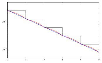
Figure 1: Plot of the asymptotic $L^{1}$ error against the log-rate (more precisely, plot of $\inf\{2^{-R_{2}(Q_{s})-2}:s>0,\,R_{0}(Q_{s})\leq x\}$ against $x$) for the BMRQ $\{Q_{s}^{\mathrm{bin}}\}$ (black), the DBMRQ $\{Q_{s}^{\mathrm{di}}\}$ (red), and the BBMRQ $\{Q_{s}^{\mathrm{bias},\alpha}\}$ for $\alpha$ close to $1/2$ (blue). We can see that the BBMRQ provides a smoother trade-off between the error and the rate (the log plot is a straight line due to scale invariance). Also, the BBMRQ outperforms the BMRQ and DBMRQ except when the log rate is close to an integer.

In this paper, we introduce an asymptotically scale-invariant multi-resolution quantizer, called the biased binary multi-resolution quantizer (BBMRQ), that performs uniformly across any choice of average quantization step (BBMRQ is a non-uniform quantizer), when the length of the range of input numbers tends to infinity. Therefore its performance degrades gracefully when the adversary modifies the communication constraints. We show that the BBMRQ outperforms the BMRQ except when the average quantization step is close to a power of $2$ (see Figure 1).

Asymptotically scale-invariant multi-resolution quantizers are also useful in successive refinement settings. Consider the scenario where an encoder observes a number $x$ and produces a sequence of bits. Due to storage or communication constraint, we only keep the first $n$ bits and discard the rest, where $n$ is chosen according to the storage constraint and the bit sequence. The BMRQ corresponds to the scheme where the bit sequence is the binary representation of $x$, and $n$ is chosen only according to the storage constraint. For the BBMRQ, $n$ also depends on the bit sequence (i.e., it is a variable length code), which allows the performance of the quantizer to vary smoothly when the storage constraint changes. The bit sequence can be produced according to the quantization tree (see Figure 2).

This paper is organized as follows. In Section II, we give the criteria of multi-resolution quantizers and define the cell size cdf for measuring the performance of a quantizer. In Section IV, we define the BBMRQ and present the main result regarding the performance of BBMRQ. In Section V, we show that the BBMRQ achieves a tradeoff between rate and error that is arbitrarily close to the optimum.

I-A Previous Work

The seminal work by Equitz and Cover [2] concerns the problem of successive refinement of information, where the lossy reconstruction is iteratively refined by supplying more information. It is also studied by Rimoldi [3]. Also see [1] for a related setting. Another line of research is multiple description coding [10, 11, 12], where several descriptions are produced from the same source, and the distortion of the reconstruction depends on which subset of descriptions is available to the decoder. Also see [13] for a related setting. Note that the aforementioned papers concern the asymptotic rate-distortion problem, whereas this paper focuses on the one-shot scalar quantization setting.

Vaishampayan [14] studied multiple description scalar quantizers. Brunk and Farvardin [4] and Jafarkhani, Brunk, and Farvardin [5] studied multi-resolution scalar quantizers (or successively refinable quantizers), and provide algorithms for designing quantizers with small error given the distribution of the input. Effros [6] and Effros and Dugatkin [9] studied multi-resolution vector quantizers. Algorithms for multi-resolution quantization were studied by Wu and Dumitrescu [7, 8]. Note that the aforementioned papers concern the setting where the distribution of the input is known, and the quantizers are designed accordingly (as in the classical Lloyd-Max algorithm [15, 16]). In this paper, we do not design the quantizer according to the input distribution, but rather assume the input is (loosely speaking) uniform over a long interval.

II Multi-resolution Quantizer

In this paper, quantizer can refer to any measurable function $Q:\mathbb{R}\to\mathbb{R}$, where the range $Q(\mathbb{R})$ is a finite or countable set. We call $Q$ a centered quantizer if each reconstruction level is the center of its corresponding quantization cell, which is formally defined below.

Definition 1.

We call a function $Q:\mathbb{R}\to\mathbb{R}$ a centered quantizer if it is non-decreasing, the range $Q(\mathbb{R})$ is a finite or countable, and

$$Q(x) =\frac{1}{2}\Big{(}\inf\{y:Q(y)\!=\!Q(x)\}+\sup\{y:Q(y)\!=\!Q(x)\}\Big{)}$$

for all $x\in\mathbb{R}$.

We give the criteria of multi-resolution quantizers below.

Definition 2.

We call $\{Q_{s}\}_{s>0}$ a multi-resolution quantizer (MRQ) if the functions $Q_{s}:\mathbb{R}\to\mathbb{R}$ are measurable and satisfy

$$Q_{s_{2}}(Q_{s_{1}}(x))=Q_{s_{2}}(x)$$

for any $s_{2}\geq s_{1}>0$ and $x\in\mathbb{R}$. The parameter $s$ (that can be any positive real number) usually corresponds to the (maximum or average) quantization step. We call $\{Q_{s}\}_{s>0}$ a centered multi-resolution quantizer if the functions $Q_{s}$ are centered quantizers.

This definition ensures that $Q_{s_{2}}(x)$ can be computed using $Q_{s_{1}}(x)$ for $s_{2}\geq s_{1}>0$, simply by quantizing $Q_{s_{1}}(x)$ using $Q_{s_{2}}$. As a result, if $s_{n}\geq s_{i}$ for all $i=1,\ldots,n$, then $Q_{s_{n}}(Q_{s_{n-1}}(\cdots Q_{s_{1}}(x)\cdots))=Q_{s_{n}}(x)$, i.e., we can quantize the final output of the relay again by the coarsest quantizer to obtain a result the same as if the input is only compressed once by the coarsest quantizer.

We remark that this definition is different from the previous definitions (e.g. [4, 5, 7]), which also concern how the quantized number is represented (e.g. by a bit sequence). Here we only concern the mapping from the input number to its reconstruction level, and assume that a suitable compression algorithm is applied to the reconstruction levels if the multi-resolution quantizer is to be used in practice.

Note that the simple uniform quantizer $Q_{s}(x):=s(\lfloor x/s\rfloor+1/2)$ is not a multi-resolution quantizer, since $Q_{3}(x)$ cannot be deduced from $Q_{2}(x)$. Nevertheless, if we restrict the step size to powers of $2$, i.e., $Q_{s}^{\mathrm{bin}}(x):=2^{\lfloor\log_{2}s\rfloor}(\lfloor 2^{-\lfloor\log_{2}s\rfloor}x\rfloor+1/2)$, then this is a MRQ, which we call the binary multi-resolution quantizer (BMRQ).

A downside of the BMRQ is that it is scale-dependent. The average absolute error of the binary multi-resolution quantizer is $2^{\lfloor\log_{2}s\rfloor-2}$ (when the input is uniformly distributed over a long interval), which must be a power of $2$. Therefore, the quantizer is suitable if the maximum allowed average absolute error is a power of $2$, but not suitable if the maximum allowed average absolute error is slightly smaller than a power of $2$. Scale-dependence is particularly undesirable in worst case or adversarial settings, where the quantizer must work well for any maximum allowed average absolute error (or other error metrics).

Loosely speaking, the BMRQ is the optimal uniform multi-resolution quantizer (where for each $s$, $Q_{s}$ divides the real line into intervals of the same length) . Nevertheless, scale-dependence is an inherent disadvantage of uniform multi-resolution quantizers. In order to overcome this disadvantage, we consider non-uniform quantizers, where each quantization cell can have different size. The distribution of cell sizes is captured by the following definition.

Definition 3.

For a (not necessarily centered) quantizer $Q:\mathbb{R}\to\mathbb{R}$, define its cell size cumulative distribution function (cell size cdf) on the measurable set $S\subseteq\mathbb{R}$ with positive measure as

$$F_{Q,S}(z) :=\frac{\lambda\left(\left\{x\in S:\,\lambda\left(\left\{y\in S:\,Q(y)=Q(x)\right\}\right)\leq z\right\}\right)}{\lambda(S)},$$

where $\lambda$ denotes the Lebesgue measure. Define its asymptotic cell size cdf $F_{Q}$ to be the cdf that is the limit (with respect to the Lévy metric) of $F_{Q,[x_{0},x_{1}]}$ as $x_{1}-x_{0}\to\infty$, i.e., $F_{Q}$ is a cdf and

$$\lim_{l\to\infty}\sup_{(x_{0},x_{1}):x_{1}-x_{0}\geq l}d_{\mathrm{L}}(F_{Q,[x_{0},x_{1}]},F_{Q})=0,$$ (1)

where $d_{\mathrm{L}}(F,G):=\inf\{\epsilon>0:F(x-\epsilon)-\epsilon\leq G(x)\leq F(x+\epsilon)+\epsilon\,\forall\,x\in\mathbb{R}\}$ is the Lévy metric. Note that $F_{Q}$ may not exist for some $Q$.

We then give the criteria for asymptotic scale invariance.

Definition 4.

For a multi-resolution quantizer $\{Q_{s}\}_{s>0}$, if $F_{Q_{s}}$ exists for any $s>0$, define

$$\overline{F}_{\{Q_{s}\}_{s}}(x) :=\sup_{s>0}\{F_{Q_{s}}(xs)\},$$

$$\text{$\underline{F}$}_{\{Q_{s}\}_{s}}(x) :=\inf_{s>0}\{F_{Q_{s}}(xs)\}.$$

We call $\{Q_{s}\}_{s>0}$ asymptotically scale-invariant if $\overline{F}_{\{Q_{s}\}_{s}}=\text{$\underline{F}$}_{\{Q_{s}\}_{s}}$, i.e., the functions $x\mapsto F_{Q_{s}}(xs)$ are the same for all $s>0$.

One way to improve the BMRQ is to add more intermediate steps between $Q_{2^{n}}^{\mathrm{bin}}$ and $Q_{2^{n+1}}^{\mathrm{bin}}$, where only some of the adjacent pairs of quantization cells of $Q_{2^{n}}^{\mathrm{bin}}$ are merged.

Definition 5.

Define the dithered binary multi-resolution quantizer (DBMRQ) as

$$Q_{s}^{\mathrm{di}}(x) :=\!\!\begin{cases}2^{\lfloor\log_{2}s\rfloor+1}(\lfloor 2^{-\lfloor\log_{2}s\rfloor-1}x\rfloor\!+\!1/2)\\ \;\;\;\;\;\hbox to0.0pt{$\displaystyle\mathrm{if}\,\mathrm{frac}(\phi\lfloor 2^{-\lfloor\log_{2}s\rfloor-1}x\rfloor)<2\!-\!2^{\lfloor\log_{2}s\rfloor+1}/s$\hss}\\ 2^{\lfloor\log_{2}s\rfloor}(\lfloor 2^{-\lfloor\log_{2}s\rfloor}x\rfloor+1/2)&\mathrm{otherwise},\end{cases}$$

where $\mathrm{frac}(\gamma):=\gamma-\lfloor\gamma\rfloor$, and $\phi:=(1+\sqrt{5})/2$ is the golden ratio (or any irrational number works).

See Figure 2 for an illustration of DBMRQ. The quantizer $Q_{s}^{\mathrm{di}}$ has two cell sizes: $2^{\lfloor\log_{2}s\rfloor}$ and $2^{\lfloor\log_{2}s\rfloor+1}$. The choice of which cell size to use is determined by the $\mathrm{frac}$ function in the definition. It can be checked that the cell size cdf of $Q_{s}^{\mathrm{di}}$ is

$$F_{Q_{s}^{\mathrm{di}}}(x) =(2-2^{\lfloor\log_{2}s\rfloor+1}/s)\mathbf{1}\{2^{(\lfloor\log_{2}s\rfloor+1)}\leq x\}$$

$$\;\;\;+(2^{\lfloor\log_{2}s\rfloor+1}/s-1)\mathbf{1}\{2^{\lfloor\log_{2}s\rfloor}\leq x\}.$$

Note that the BMRQ and the DBMRQ are not asymptotically scale-invariant.

III Quantities of Interest

The cell size cdf provides some information about the quantizer $Q$. We define the following useful quantity.

Definition 6.

For a quantizer $Q$ where $F_{Q}$ exists, define its Rényi entropy rate as

$$R_{\eta}(Q):=\frac{1}{1-\eta}\log_{2}\int_{0}^{\infty}\gamma^{\eta-1}\mathrm{d}F_{Q}(\gamma)$$

for $\eta\in\mathbb{R}_{>0}\backslash\{1\}$, and

$$R_{1}(Q):=\int_{0}^{\infty}\log_{2}(\gamma^{-1})\mathrm{d}F_{Q}(\gamma).$$

We call $R_{0}(Q)$ the log-rate of $Q$.

Several quanities of interest can be obtained from the Rényi entropy rate. If $X\sim\mathrm{Unif}[x_{0},x_{1}]$, then:

• The number of reconstruction levels (possible values of $Q(X)$ with positive probability) is

  $$|\{x:\,\mathbf{P}(Q(X)=x)>0\}|=(x_{1}-x_{0})\int_{0}^{\infty}\gamma^{-1}\mathrm{d}F_{Q,[x_{0},x_{1}]}(\gamma).$$

  The reason is that for a quantization cell of size $\gamma$, the probability that $X$ is in that cell is $\gamma/(x_{1}-x_{0})$, and hence its contribution to $(x_{1}-x_{0})\int_{0}^{\infty}\gamma^{-1}\mathrm{d}F_{Q,[x_{0},x_{1}]}(\gamma)$ is $(x_{1}-x_{0})\gamma^{-1}(\gamma/(x_{1}-x_{0}))=1$. Hence, the number of bits needed to encode the levels (using fixed-length code) is $\lceil\log_{2}((x_{1}-x_{0})\int_{0}^{\infty}\gamma^{-1}\mathrm{d}F_{Q,[x_{0},x_{1}]}(\gamma))\rceil$. Therefore, the log-rate

  $$R_{0}(Q)=\log_{2}\int_{0}^{\infty}\gamma^{-1}\mathrm{d}F_{Q}(\gamma)$$

  is the logarithm of the rate of increase of the number of reconstruction levels as the interval $[x_{0},x_{1}]$ becomes longer.

• The entropy of the output is

  $$H(Q(X))=\int_{0}^{\infty}\log_{2}(\gamma^{-1}(x_{1}-x_{0}))\mathrm{d}F_{Q,[x_{0},x_{1}]}(\gamma).$$

  Therefore,

  $$R_{1}(Q)=\int_{0}^{\infty}\log_{2}(\gamma^{-1})\mathrm{d}F_{Q}(\gamma)$$

  describes how $H(Q(X))$ increases as the interval $[x_{0},x_{1}]$ becomes longer.

• The average $L^{p}$ error is lower-bounded by

  $$\mathbf{E}[|X\!-\!Q(X)|^{p}]\geq\int_{0}^{\infty}\frac{(\gamma/2)^{p}}{p+1}\mathrm{d}F_{Q,[x_{0},x_{1}]}(\gamma).$$ (2)

  The reason is that for a quantization cell of size $\gamma$, the expected $L^{p}$ error conditioned on that $X$ is in that cell is at least $(\gamma/2)^{p}/(p+1)$ (equality holds if the quantization cell is an interval, and the reconstruction level is its midpoint). The following proposition shows the relation between the asymptotic $L^{p}$ error and $R_{p+1}(Q)$.

Proposition 7.

Fix $p>0$ and a quantizer $Q$ where $F_{Q}$ exists. Let $X\sim\mathrm{Unif}[x_{0},x_{1}]$. We have

$$\underset{x_{1}-x_{0}\to\infty}{\lim\inf}\mathbf{E}[|X-Q(X)|^{p}]\geq\frac{1}{p+1}2^{-p(R_{p+1}(Q)+1)}.$$

Moreover, if $Q$ is centered, then

$$\lim_{x_{1}-x_{0}\to\infty}\mathbf{E}[|X-Q(X)|^{p}]=\frac{1}{p+1}2^{-p(R_{p+1}(Q)+1)}.$$

Proof:

For the first part, if $x_{1}-x_{0}\to\infty$, then $F_{Q,[x_{0},x_{1}]}\to F_{Q}$ (in Lévy metric), and hence by (2),

$$\underset{x_{1}-x_{0}\to\infty}{\lim\inf}\mathbf{E}[|X\!-\!Q(X)|^{p}]$$

$$\geq\underset{x_{1}-x_{0}\to\infty}{\lim\inf}\int_{0}^{\infty}\frac{(\gamma/2)^{p}}{p+1}\mathrm{d}F_{Q,[x_{0},x_{1}]}(\gamma)$$

$$\geq\int_{0}^{\infty}\frac{(\gamma/2)^{p}}{p+1}\mathrm{d}F_{Q}(\gamma)$$

$$=\frac{1}{p+1}2^{-p(R_{p+1}(Q)+1)}.$$

For the second part, assume that $Q$ is centered. We first show that there exists $b>0$ such that each quantization cell has size upper-bounded by $b$. Assume the contrary that the quantization cells can be arbitrarily large. Then there exists a sequence $\{(x_{0,i},x_{1,i})\}_{i}$ such that $x_{1,i}-x_{0,i}\to\infty$ and $F_{Q,[x_{0,i},x_{1,i}]}(\gamma)=\mathbf{1}\{\gamma\geq x_{1,i}-x_{0,i}\}$ (take $x_{0,i},x_{1,i}$ to be the end points of cells in a sequence of cells with sizes tend to $\infty$). This contradicts (1) since $F_{Q,[x_{0,i},x_{1,i}]}$ does not have a limit. Hence such $b>0$ exists. For $X\sim\mathrm{Unif}[x_{0},x_{1}]$, we have

$$\mathbf{E}[|X-Q(X)|^{p}]$$

$$\leq\mathbf{E}\left[\mathbf{1}\{X\in[x_{0}+b,\,x_{1}-b]\}|X-Q(X)|^{p}\right]+\mathbf{P}\left(X\notin[x_{0}+b,\,x_{1}-b]\right)\frac{(b/2)^{p}}{p+1}$$

$$\leq\int_{0}^{\infty}\frac{(\gamma/2)^{p}}{p+1}\mathrm{d}F_{Q,[x_{0},x_{1}]}(\gamma)+\frac{2b}{x_{1}-x_{0}}\cdot\frac{(b/2)^{p}}{p+1}$$

$$\to\int_{0}^{\infty}\frac{(\gamma/2)^{p}}{p+1}\mathrm{d}F_{Q}(\gamma)\,=\,\frac{1}{p+1}2^{-p(R_{p+1}(Q)+1)}$$

as $x_{1}-x_{0}\to\infty$. ∎

IV Biased Binary Multi-resolution Quantizer

We now state the main result in this paper, which is proved later in this section.

Theorem 8.

For any $\epsilon>0$, there exists an asymptotically scale-invariant centered MRQ $\{Q_{s}\}_{s>0}$ with $\overline{F}_{\{Q_{s}\}_{s}}(1/2-\epsilon)=0$, $\overline{F}_{\{Q_{s}\}_{s}}(1)=1$, and $d_{\mathrm{L}}(\overline{F}_{\{Q_{s}\}_{s}},F_{2^{\mathrm{Unif}[-1,0]}})<\epsilon$, where

$$F_{2^{\mathrm{Unif}[-1,0]}}(x):=\min\left\{\max\{\log_{2}(x)+1,\,0\},\,1\right\},$$

i.e., $F_{2^{\mathrm{Unif}[-1,0]}}$ is the cdf of $2^{Z}$ where $Z\sim\mathrm{Unif}[-1,0]$.

As a result, the Rényi entropy rate $R_{\eta}(Q_{s})$ can be arbitrarily close to

$$\frac{1}{1-\eta}\log_{2}\left(\frac{1-2^{1-\eta}}{\eta-1}\log_{2}e\right)-\log_{2}s$$ (3)

for $\eta\neq 1$, and $R_{1}(Q_{s})$ can be arbitrarily close to $1/2-\log_{2}s$. We will show in Corollary 11 that this tradeoff between log-rate and $L^{p}$ error can be arbitrarily close to optimal.

To prove Theorem 8, we introduce the following construction.

Definition 9.

We define the biased quantization tree with parameter $0<\alpha<1$ recursively as follows. For any $n\in\mathbb{Z}$ and sequence $\{z_{i}\}_{i\leq n}$ ($z_{i}\in\{0,1\}$, the index $i$ is over $\mathbb{Z}\cap(-\infty,n]$) with finitely many $1$’s, define

$$(\text{$\underline{T}$}_{n}^{\mathrm{bias},\alpha}(\{z_{i}\}_{i\leq n}),\overline{T}_{n}^{\mathrm{bias},\alpha}(\{z_{i}\}_{i\leq n}))$$

$$\!:=\!\begin{cases}\left(0,\,\alpha^{n}\right)&\!\!\!\!\!\!\!\!\!\!\!\!\!\!\!\!\!\!\mathrm{if}\,z_{n}\!=\!z_{n-1}\!=\!\cdots\!=\!0\\ \left(\text{$\underline{T}$}_{n-1},\alpha\overline{T}_{n-1}\!+\!(1\!-\!\alpha)\text{$\underline{T}$}_{n-1}\right)&\mathrm{else}\,\mathrm{if}\;z_{n}=0\\ \left(\alpha\overline{T}_{n-1}\!+\!(1\!-\!\alpha)\text{$\underline{T}$}_{n-1},\overline{T}_{n-1}\right)&\mathrm{otherwise}.\end{cases}$$

where we write $\overline{T}_{n-1}=\overline{T}_{n-1}^{\mathrm{bias},\alpha}(\{z_{i}\}_{i\leq n-1})$ (likewise for $\text{$\underline{T}$}_{n-1}$) for brevity. Note that the first case above serves as the base case of the recursive definition.

Define the biased binary multi-resolution quantizer (BBMRQ) with parameter $0<\alpha<1$ as follows. For $x\geq 0$, define

$$Q_{s}^{\mathrm{bias},\alpha}(x) :=\frac{1}{2}\left(\text{$\underline{T}$}_{n}^{\mathrm{bias},\alpha}(\{z_{i}\}_{i\leq n})+\overline{T}_{n}^{\mathrm{bias},\alpha}(\{z_{i}\}_{i\leq n})\right),$$

where $\{z_{i}\}_{i\leq n}$ satisfies $x\in[\text{$\underline{T}$}_{n}^{\mathrm{bias},\alpha}(\{z_{i}\}_{i\leq n}),\overline{T}_{n}^{\mathrm{bias},\alpha}(\{z_{i}\}_{i\leq n}))$ and $\overline{T}_{n}^{\mathrm{bias},\alpha}(\{z_{i}\}_{i\leq n})-\text{$\underline{T}$}_{n}^{\mathrm{bias},\alpha}(\{z_{i}\}_{i\leq n})\leq s$, and we select the $\{z_{i}\}_{i\leq n}$ with the smallest $n$ satisfying these two constraints. For $x<0$, define $Q_{s}^{\mathrm{bias},\alpha}(x):=-Q_{s}^{\mathrm{bias},\alpha}(-x)$.

Intuitively, the BBMRQ repeatedly divides an interval into two subintervals of proportion $\alpha$ and $1-\alpha$, until the lengths of the intervals fall below $s$ (see Figure 2). It is clear that the BBMRQ is a centered MRQ.

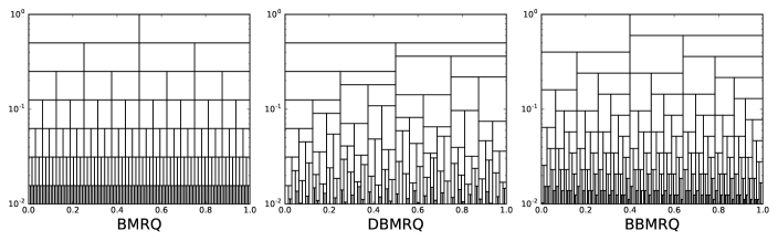
Figure 2: The quantization tree of BMRQ, DBMRQ and BBMRQ (from left to right). The x-axis is the input $x$, and the y-axis is the parameter $s$. A rectangle in the figure means that each point $(x,s)$ in the rectangle has the same quantized value $Q_{s}(x)$.

We then use the BBMRQ to prove Theorem 8.

Proof:

Fix any $1/2<\alpha<3/4$ such that $(\ln\alpha)/(\ln(1-\alpha))$ is irrational. Write $Q_{s}=Q_{s}^{\mathrm{bias},\alpha}$ for brevity. Let $X\sim\mathrm{Unif}[0,1]$, and

$$W_{t}:=2^{t}\lambda\left(\left\{y:\,Q_{2^{-t}}(y)=Q_{2^{-t}}(X)\right\}\right)$$

for $t\geq 0$, where $\lambda$ denotes the Lebesgue measure. Note that $-\log_{2}W_{t}$ is the residual life of a renewal process with interarrival time distribution $\alpha\delta_{-\log_{2}\alpha}+(1-\alpha)\delta_{-\log_{2}(1-\alpha)}$, where $\delta_{w}$ is the degenerate distribution at $w$ (as $t$ increases, each time the quantization cell containing $X$ splits into two, there is a probability $\alpha$ for $X$ to be in the cell with proportion $\alpha$, and a probability $1-\alpha$ for $X$ to be in the cell with proportion $1-\alpha$). Since $(\ln\alpha)/(\ln(1-\alpha))$ is irrational, the interarrival times have a non-lattice distribution. Denote the Markov kernel (conditional distribution of $W_{s+t}$ given $W_{s}$) as $\kappa_{\alpha}^{t}$. By the key renewal theorem [17], we have

$$d_{\mathrm{L}}(\kappa_{\alpha}^{t}\delta_{1},F_{\mathrm{bias},\alpha})\to 0$$

as $t\to\infty$, where $\kappa_{\alpha}^{t}\delta_{1}$ denotes the distribution of $W_{t}$ conditioned on $W_{0}=1$, and $F_{\mathrm{bias},\alpha}$ is the cdf of the stationary distribution of the process $\{W_{t}\}$, given by

$$F_{\mathrm{bias},\alpha}(\gamma) :=\left(-\alpha\log_{2}\alpha-(1-\alpha)\log_{2}(1-\alpha)\right)^{-1}$$

$$\;\;\;\cdot\Big{(}\alpha\max\left\{\log_{2}(\min\{\gamma,1\}/\alpha),0\right\}$$

$$\;\;\;\;\;+(1\!-\!\alpha)\max\left\{\log_{2}(\min\{\gamma,1\}/(1\!-\!\alpha)),0\right\}\!\Big{)}.$$ (4)

For $\tau>0$, let $\epsilon_{\tau}$ be such that $d_{\mathrm{L}}(\kappa_{\alpha}^{t}\delta_{1},F_{\mathrm{bias},\alpha})\leq\epsilon_{\tau}$ for all $t\geq\tau$, and $\epsilon_{\tau}\to 0$ as $\tau\to\infty$.

Fix any $s>0$, $\tau>1$ and $l>\tau 2^{\tau+3}s$. Fix any $x_{0},x_{1}$ such that $x_{1}-x_{0}\geq l$. Let $X\sim\mathrm{Unif}[x_{0},x_{1}]$. Let $[\text{$\underline{T}$}_{n^{(i)}}(z^{(i)}),\overline{T}_{n^{(i)}}(z^{(i)}))$ be the quantization cells of $Q_{2^{\tau+2}s}$ that are subsets of $[x_{0},x_{1}]$, where $n^{(i)}\in\mathbb{Z}$ and $z^{(i)}\in\{0,1\}^{\mathbb{Z}\cap(-\infty,n^{(i)}]}$ for $i=1,2,\ldots,\tilde{N}$. Since $X$ is not in one of $[\text{$\underline{T}$}_{n^{(i)}}(z^{(i)}),\overline{T}_{n^{(i)}}(z^{(i)}))$ only when $X$ is in a quantization cell of $Q_{2^{\tau+2}s}$ that includes $x_{0}$ or $x_{1}$, and each quantization cell of $Q_{2^{\tau+2}s}$ has length between $2^{\tau}s$ and $2^{\tau+2}s$ (since $1/2<\alpha<3/4$), we have

$$\mathbf{P}\bigg{(}\!X\notin\bigcup_{i=1}^{\tilde{N}}[\text{$\underline{T}$}_{n^{(i)}}(z^{(i)}),\overline{T}_{n^{(i)}}(z^{(i)}))\!\bigg{)} \leq\frac{2(2^{\tau+2}s)}{x_{1}-x_{0}}$$

$$\leq 1/\tau.$$

Let $W_{t}:=2^{t}\lambda(\{y:\,Q_{2^{-t}}(y)=Q_{2^{-t}}(X)\})$. Conditioned on $X\in[\text{$\underline{T}$}_{n^{(i)}}(z^{(i)}),\overline{T}_{n^{(i)}}(z^{(i)}))$ (let $L:=\overline{T}_{n^{(i)}}(z^{(i)})-\text{$\underline{T}$}_{n^{(i)}}(z^{(i)})$), we have $W_{-\log_{2}L}=1$, and $\{W_{t}\}_{t\geq-\log_{2}L}$ is a stochastic process with Markov kernel $\kappa_{\alpha}^{t}$, and thus $W_{-\log_{2}s}\sim\kappa_{\alpha}^{\log_{2}L-\log_{2}s}\delta_{1}$, and $d_{\mathrm{L}}(\kappa_{\alpha}^{\log_{2}L-\log_{2}s}\delta_{1},F_{\mathrm{bias},\alpha})\leq\epsilon_{\tau}$ since $\log_{2}L-\log_{2}s\geq\log_{2}2^{\tau}s-\log_{2}s=\tau$. Let $\bar{W}:=s^{-1}\lambda(\{y\in[x_{0},x_{1}]:\,Q_{s}(y)=Q_{s}(x)\})$. Since $\bar{W}=W_{-\log_{2}s}$ if $X\in\bigcup_{i=1}^{\tilde{N}}[\text{$\underline{T}$}_{n^{(i)}}(z^{(i)}),\overline{T}_{n^{(i)}}(z^{(i)}))$, we have $d_{\mathrm{L}}(F_{\bar{W}},F_{\mathrm{bias},\alpha})<\epsilon_{\tau}+1/\tau$. Therefore $F_{\bar{W}}\to F_{\mathrm{bias},\alpha}$ as $\tau\to\infty$, and thus $\{Q_{s}\}$ is asymptotically scale-invariant with cell size cdf $F_{\mathrm{bias},\alpha}$. The result follows from the fact that $d_{\mathrm{L}}(F_{\mathrm{bias},\alpha},F_{2^{\mathrm{Unif}[-1,0]}})\to 0$ as $\alpha\to 1/2$. ∎

V Converse Results

In this section, we show a fundamental tradeoff between the log-rate and the $L^{p}$ error of asymptotically scale-invariant multi-resolution quantizers, and that BBMRQ can be arbitrarily close to optimal in this regard. We first show an inequality that must be satisfied by all asymptotically scale-invariant multi-resolution quantizers.

Theorem 10.

For any asymptotically scale-invariant multi-resolution quantizer $\{Q_{s}\}_{s>0}$ with finite log-rate (i.e., $R_{0}(Q_{1})=\log_{2}\int_{0}^{\infty}\gamma^{-1}\mathrm{d}\overline{F}(\gamma)<\infty$, where we write $\overline{F}=\overline{F}_{\{Q_{s}\}_{s}}$), the distribution given by the cdf $\overline{F}$ is a continuous distribution, and its pdf $\bar{f}$ satisfies

$$\int_{0}^{\infty}x^{-1}\left(1+\mathbf{1}\left\{\overline{f}(x)\geq\zeta\overline{f}(x\zeta)\right\}\right)\left(\overline{f}(x)-\zeta\overline{f}(x\zeta)\right)\mathrm{d}x\leq 0$$ (5)

for any $\zeta>1$. As a result,

$$\bar{f}(y)\leq\int_{0}^{\infty}x^{-1}\left(1+\mathbf{1}\{x>y\}\right)\bar{f}(x)\mathrm{d}x$$ (6)

for almost all $y>0$.

Proof:

Let $p_{s,\gamma}$ be the probability mass function corresponding to the cdf $F_{Q_{s},[-\gamma,\gamma]}$ for $\gamma>0$ (note that it is a discrete distribution so pmf exists). The number of quantization cells of $Q_{s}$ in $[-\gamma,\gamma]$ of size $x$ is $2\gamma x^{-1}p_{s,\gamma}(x)$. Let $n_{x}$ (resp. $\tilde{n}_{x}$) be the number of quantization cells of $Q_{s}$ (resp. $Q_{s/\gamma}$) in $[-\gamma,\gamma]$ of size $x$ that are not quantization cells of $Q_{s/\gamma}$ (resp. $Q_{s}$). We have $n_{x}-\tilde{n}_{x}=2\gamma x^{-1}(p_{s,\gamma}(x)-p_{s/\zeta,\gamma}(x))$. Since each cell of $Q_{s}$ is split into 2 or more cells in $Q_{s/\gamma}$, we have $2\sum_{x}n_{x}\leq\sum_{x}\tilde{n}_{x}$ (the summation is over $x$ in the support of $p_{s,\gamma}$ or $p_{s/\zeta,\gamma}$), and hence

$$2\sum_{x:\,p_{s,\gamma}(x)>p_{s/\zeta,\gamma}(x)}x^{-1}(p_{s,\gamma}(x)-p_{s/\zeta,\gamma}(x))$$

$$=2\gamma^{-1}\sum_{x:\,n_{x}>\tilde{n}_{x}}(n_{x}-\tilde{n}_{x})$$

$$=\gamma^{-1}\left(2\sum_{x}n_{x}-2\sum_{x}\min\{n_{x},\tilde{n}_{x}\}\right)$$

$$\leq\gamma^{-1}\left(\sum_{x}\tilde{n}_{x}-2\sum_{x}\min\{n_{x},\tilde{n}_{x}\}\right)$$

$$\leq\gamma^{-1}\sum_{x:\,n_{x}<\tilde{n}_{x}}(\tilde{n}_{x}-n_{x})$$

$$=\sum_{x:\,p_{s,\gamma}(x)<p_{s/\zeta,\gamma}(x)}x^{-1}(p_{s/\zeta,\gamma}(x)-p_{s,\gamma}(x)).$$ (7)

Let $\nu$ be the signed measure induced by $\overline{F}(x)-\overline{F}(x\zeta)$ (i.e., $\nu(B)=\int_{B}\mathrm{d}(\overline{F}(x)-\overline{F}(x\zeta))$). Fix any $\epsilon>0$. Let $A\subseteq\mathbb{R}_{>0}$ be a measurable set. Since the measure $B\mapsto\int_{B}x^{-1}\mathrm{d}(\overline{F}(x)+\overline{F}(x\zeta))$ is a regular measure over $\mathbb{R}_{>0}$ , there exists an open set $A^{\prime}$ such that $A\subseteq A^{\prime}$ and $\int_{A^{\prime}\backslash A}x^{-1}\mathrm{d}(\overline{F}(x)+\overline{F}(x\zeta))<\epsilon$. Since $A^{\prime}$ is open, it can be expressed as a countable disjoint union of open intervals $A^{\prime}=\bigcup_{i}(a_{i},b_{i})$. Let $A^{\prime}_{\delta}:=\bigcup_{i}(a_{i}+\delta,b_{i}-\delta)$ for $\delta>0$ (where $(a_{i}+\delta,b_{i}-\delta)=\emptyset$ if $a_{i}+\delta\geq b_{i}-\delta$). Let $g_{\delta}(x):=\min\{(x-a_{i})\delta^{-1},\,(b_{i}-x)\delta^{-1},\,1\}$ if $x\in(a_{i},b_{i})$ ($g_{\delta}(x)=0$ if $x$ is not in any of those invervals). Then $g_{\delta}$ is continuous and $\mathbf{1}\{x\in A^{\prime}_{\delta}\}\leq g_{\delta}(x)\leq\mathbf{1}\{x\in A^{\prime}\}$. Hence,

$$\int_{A}x^{-1}\nu(\mathrm{d}x)$$

$$\leq\int_{A^{\prime}}x^{-1}\nu(\mathrm{d}x)+\int_{A^{\prime}\backslash A}x^{-1}\mathrm{d}(\overline{F}(x)+\overline{F}(x\zeta))$$

$$\leq\int x^{-1}g_{\delta}(x)\nu(\mathrm{d}x)+\int_{A^{\prime}\backslash A^{\prime}_{\delta}}x^{-1}\mathrm{d}(\overline{F}(x)+\overline{F}(x\zeta))+\epsilon$$

$$\to\int x^{-1}g_{\delta}(x)\nu(\mathrm{d}x)+\epsilon$$

as $\delta\to 0$ since $A^{\prime}_{\delta}\nearrow A^{\prime}$. Also,

$$\int_{A}x^{-1}\nu(\mathrm{d}x)$$

$$\geq\int_{A^{\prime}}x^{-1}\nu(\mathrm{d}x)$$

$$\geq\int x^{-1}g_{\delta}(x)\nu(\mathrm{d}x)-\int_{A^{\prime}\backslash A^{\prime}_{\delta}}x^{-1}\mathrm{d}(\overline{F}(x)+\overline{F}(x\zeta))$$

$$\to\int x^{-1}g_{\delta}(x)\nu(\mathrm{d}x)$$

as $\delta\to 0$. Therefore, we can let $g:=g_{\delta}$ for a $\delta>0$ small enough that

$$\left|\int_{A}x^{-1}\nu(\mathrm{d}x)-\int x^{-1}g(x)\nu(\mathrm{d}x)\right|<2\epsilon.$$ (8)

Since $F_{Q_{s},[-\gamma,\gamma]}\to\overline{F}$ as $\gamma\to\infty$, and $x\mapsto 1+g(x)$ is bounded and continuous, we have $\int x^{-1}(1+g(x))\mathrm{d}F_{Q_{1},[-\gamma,\gamma]}(x)\to\int x^{-1}(1+g(x))\mathrm{d}\overline{F}(x)$. Also, $\int x^{-1}(1+g(x))\mathrm{d}F_{Q_{1/\zeta},[-\gamma,\gamma]}(x)\to\int x^{-1}(1+g(x))\mathrm{d}\overline{F}(x\zeta)$. As a result,

$$\int x^{-1}(1+g(x))\mathrm{d}\big{(}F_{Q_{1},[-\gamma,\gamma]}(x)-F_{Q_{1/\zeta},[-\gamma,\gamma]}(x)\big{)}$$

$$\to\int x^{-1}(1+g(x))\mathrm{d}\big{(}\overline{F}(x)-\overline{F}(x\zeta)\big{)}$$

$$=\int x^{-1}(1+g(x))\nu(\mathrm{d}x).$$ (9)

It can be deduced from (7) that

$$\sum_{x}x^{-1}(1+\tilde{g}(x))(p_{s,\gamma}(x)-p_{s/\zeta,\gamma}(x))\leq 0$$

for any $\tilde{g}:\mathbb{R}_{>0}\to[0,1]$, where the summation is over $x$ in the support of $p_{s,\gamma}$ or $p_{s/\zeta,\gamma}$ (because to maximize the above expression, we should assign $\tilde{g}(x)=0$ to $x$’s where $p_{s/\zeta,\gamma}(x)-p_{s,\gamma}(x)>0$, and $\tilde{g}(x)=1$ otherwise). Substituting $\tilde{g}=g$,

$$\int x^{-1}(1+g(x))\mathrm{d}\big{(}F_{Q_{1},[-\gamma,\gamma]}(x)-F_{Q_{1/\zeta},[-\gamma,\gamma]}(x)\big{)}\leq 0.$$

By (9),

$$\int x^{-1}(1+g(x))\nu(\mathrm{d}x)\leq 0.$$

By (8),

$$\int x^{-1}\nu(\mathrm{d}x)+\int_{A}x^{-1}\nu(\mathrm{d}x)\leq 2\epsilon.$$

Taking $\epsilon\to 0$ and rearranging the terms,

$$\int x^{-1}(1+\mathbf{1}\{x\in A\})\nu(\mathrm{d}x)\leq 0,$$ (10)

$$\int_{0}^{\infty}x^{-1}(1+\mathbf{1}\{x\in A\})\mathrm{d}\overline{F}(x)\leq\zeta\int_{0}^{\infty}x^{-1}(1+\mathbf{1}\{x/\zeta\in A\})\mathrm{d}\overline{F}(x),$$

$$\int_{0}^{\infty}x^{-1}(1+\mathbf{1}\{x\in A\}-\zeta-\zeta\mathbf{1}\{x/\zeta\in A\})\mathrm{d}\overline{F}(x)\leq 0.$$

Substituting $A=\{x:\,x>y\}$,

$$0 \geq\int_{0}^{\infty}x^{-1}(1+\mathbf{1}\{x>y\}-\zeta-\zeta\mathbf{1}\{x>y\zeta\})\mathrm{d}\overline{F}(x)$$

$$=\int_{0}^{\infty}x^{-1}\left(\mathbf{1}\{y<x\leq y\zeta\}-(\zeta-1)\left(1+\mathbf{1}\{x>y\zeta\}\right)\right)\mathrm{d}\overline{F}(x)$$

$$\geq\frac{\overline{F}(y\zeta)-\overline{F}(y)}{y\zeta}-(\zeta-1)\int_{0}^{\infty}x^{-1}\left(1+\mathbf{1}\{x>y\zeta\}\right)\mathrm{d}\overline{F}(x).$$

Hence,

$$\frac{\overline{F}(y\zeta)-\overline{F}(y)}{y\zeta-y}\leq\zeta\int_{0}^{\infty}x^{-1}\left(1+\mathbf{1}\{x>y\zeta\}\right)\mathrm{d}\overline{F}(x).$$

Since the right hand side is bounded by $\zeta 2^{R_{0}+1}$, $\bar{f}$ exists and (6) holds for almost all $y>0$. Therefore, (10) becomes

$$\int x^{-1}(1+\mathbf{1}\{x\in A\})\left(\overline{f}(x)-\zeta\overline{f}(x\zeta)\right)dx\leq 0.$$

We can obtain (5) by substituting $A=\{x:\,\overline{f}(x)\geq\zeta\overline{f}(x\zeta)\}$. ∎

As a result, we can bound the log-rate and the $L^{p}$ error of an asymptotically scale-invariant multi-resolution quantizer using the following corollary and Proposition 7.

Corollary 11.

For any asymptotically scale-invariant multi-resolution quantizer $\{Q_{s}\}_{s>0}$ with finite log-rate, for any $s>0$, $p>0$,

$$R_{0}(Q_{s})-R_{p+1}(Q_{s})\geq\frac{1}{p}\log_{2}\left(\frac{1-2^{-p}}{p}(\log_{2}e)^{p+1}\right).$$ (11)

Recall that for the BBMRQ, by (3), $R_{0}(Q_{s})$ can be arbitrarily close to $\log_{2}\log_{2}e-\log_{2}s$, and $R_{p+1}(Q_{s})$ can be arbitrarily close to

$$-\frac{1}{p}\log_{2}\left(\frac{1-2^{-p}}{p}\log_{2}e\right)-\log_{2}s.$$

Therefore the lower bound in (11) can be approached. This shows that the tradeoff between log-rate and $L^{p}$ error of BBMRQ can be arbitrarily close to optimal.

Nevertheless, it is unknown whether the lower bound in (11) can be attained exactly. It can be tracked in the proof of Corollary 11 that the equality in (11) holds if and only if there exists $s>0$ such that $\overline{F}_{\{Q_{s}\}_{s}}(\gamma)=F_{2^{\mathrm{Unif}[-1,0]}}(\gamma s)$ for all $\gamma$, i.e., Theorem 8 can be attained exactly. We conjecture that this is impossible.

Conjecture 12.

There does not exist an asymptotically scale-invariant centered MRQ $\{Q_{s}\}_{s>0}$ with $\overline{F}_{\{Q_{s}\}_{s}}=F_{2^{\mathrm{Unif}[-1,0]}}$.

We now prove Corollary 11.

Proof:

By Theorem 10, for any pdf $\psi:\mathbb{R}_{>0}\to\mathbb{R}_{\geq 0}$,

$$\int\bar{f}(y)\psi(y)\mathrm{d}y \leq\int_{0}^{\infty}\int_{0}^{\infty}x^{-1}\left(1+\mathbf{1}\{x>y\}\right)\bar{f}(x)\mathrm{d}x\cdot\psi(y)\mathrm{d}y$$

$$=\int_{0}^{\infty}x^{-1}\left(1+\int_{0}^{x}\psi(y)\mathrm{d}y\right)\bar{f}(x)\mathrm{d}x,$$

$$\int_{0}^{\infty}\left(x^{-1}\left(1+\int_{0}^{x}\psi(y)\mathrm{d}y\right)-\psi(x)\right)\bar{f}(x)\mathrm{d}x\geq 0.$$ (12)

Substitute

$$\psi(y)=\mathbf{1}\{1/2\leq y\leq 1\}\frac{(1-2^{-p})\log_{2}y-y^{p}+1}{(1-2^{-p})\left(\frac{1-\log_{2}e}{2}\right)-\frac{1-2^{-(p+1)}}{p+1}+1/2}.$$

For $1/2\leq x\leq 1$,

$$x^{-1}\left(1+\int_{0}^{x}\psi(y)\mathrm{d}y\right)-\psi(x)$$

$$=x^{-1}+\frac{x^{-1}\int_{1/2}^{x}\left((1-2^{-p})\log_{2}y-y^{p}+1\right)\mathrm{d}y-\left((1-2^{-p})\log_{2}x-x^{p}+1\right)}{(1-2^{-p})\left(\frac{1-\log_{2}e}{2}\right)-\frac{1-2^{-(p+1)}}{p+1}+1/2}$$

$$=x^{-1}+\frac{x^{-1}\left((1-2^{-p})\left(-x\log_{2}e+x\log_{2}x+(\log_{2}e)/2+1/2\right)-\frac{x^{p+1}-2^{-(p+1)}}{p+1}+x-1/2\right)-\left((1-2^{-p})\log_{2}x-x^{p}+1\right)}{(1-2^{-p})\left(\frac{1-\log_{2}e}{2}\right)-\frac{1-2^{-(p+1)}}{p+1}+1/2}$$

$$=x^{-1}+\frac{(1-2^{-p})\left(-\log_{2}e+\log_{2}x+(\log_{2}e)x^{-1}/2+x^{-1}/2\right)-\frac{x^{p}-2^{-(p+1)}x^{-1}}{p+1}+1-x^{-1}/2-(1-2^{-p})\log_{2}x+x^{p}-1}{(1-2^{-p})\left(\frac{1-\log_{2}e}{2}\right)-\frac{1-2^{-(p+1)}}{p+1}+1/2}$$

$$=x^{-1}+\frac{(1-2^{-p})\left(-\log_{2}e+(\log_{2}e)x^{-1}/2+x^{-1}/2\right)-\frac{x^{p}-2^{-(p+1)}x^{-1}}{p+1}-x^{-1}/2+x^{p}}{(1-2^{-p})\left(\frac{1-\log_{2}e}{2}\right)-\frac{1-2^{-(p+1)}}{p+1}+1/2}$$

$$=\left(1+\frac{(1-2^{-p})\left((\log_{2}e)/2+1/2\right)+\frac{2^{-(p+1)}}{p+1}-1/2}{(1-2^{-p})\left(\frac{1-\log_{2}e}{2}\right)-\frac{1-2^{-(p+1)}}{p+1}+1/2}\right)x^{-1}+\frac{(1-2^{-p})\left(-\log_{2}e\right)-\frac{x^{p}}{p+1}+x^{p}}{(1-2^{-p})\left(\frac{1-\log_{2}e}{2}\right)-\frac{1-2^{-(p+1)}}{p+1}+1/2}$$

$$=\left(\frac{\frac{p}{p+1}(1-2^{-p})}{(1-2^{-p})\left(\frac{1-\log_{2}e}{2}\right)-\frac{1-2^{-(p+1)}}{p+1}+1/2}\right)x^{-1}+\frac{(1-2^{-p})\left(-\log_{2}e\right)+x^{p}\frac{p}{p+1}}{(1-2^{-p})\left(\frac{1-\log_{2}e}{2}\right)-\frac{1-2^{-(p+1)}}{p+1}+1/2}$$

$$=\frac{\frac{p}{p+1}\left((1-2^{-p})x^{-1}+x^{p}\right)-(1-2^{-p})\log_{2}e}{(1-2^{-p})\left(\frac{1-\log_{2}e}{2}\right)-\frac{1-2^{-(p+1)}}{p+1}+1/2}$$

$$=\frac{\frac{p}{p+1}\left((1-2^{-p})x^{-1}+x^{p}\right)-(1-2^{-p})\log_{2}e}{(1-2^{-p})\left(\frac{1-\log_{2}e}{2}\right)+\frac{p/2-(1/2)(1-2^{-p})}{p+1}}$$

$$=2\cdot\frac{\frac{p}{p+1}\left((1-2^{-p})x^{-1}+x^{p}\right)-(1-2^{-p})\log_{2}e}{\frac{p}{p+1}(2-2^{-p})-(1-2^{-p})\log_{2}e}$$

For $x\geq 1$, we have

$$p\geq(1-2^{-p})\log_{2}e,$$

$$\frac{p+1}{p}\geq\frac{p+1}{p^{2}}(1-2^{-p})\log_{2}e,$$

$$x^{p+1}\geq 1 \geq\frac{p+1}{p^{2}}\left((1-2^{-p})\log_{2}e-\frac{p}{p+1}\right),$$

$$\frac{p^{2}}{p+1}x^{p-1}\geq\left((1-2^{-p})\log_{2}e-\frac{p}{p+1}\right)x^{-2}.$$

Integrating both sides from $1$ to $x$,

$$\frac{p}{p+1}(x^{p}-1)\geq\left((1-2^{-p})\log_{2}e-\frac{p}{p+1}\right)(1-x^{-1}),$$

$$\left((1-2^{-p})\log_{2}e-\frac{p}{p+1}\right)x^{-1}+\frac{p}{p+1}x^{p}-(1-2^{-p})\log_{2}e\geq 0.$$

Therefore,

$$2\cdot\frac{\frac{p}{p+1}\left((1-2^{-p})x^{-1}+x^{p}\right)-(1-2^{-p})\log_{2}e}{\frac{p}{p+1}(2-2^{-p})-(1-2^{-p})\log_{2}e}-\left(x^{-1}\left(1+\int_{0}^{x}\psi(y)\mathrm{d}y\right)-\psi(x)\right)$$

$$=2\cdot\frac{\frac{p}{p+1}\left((1-2^{-p})x^{-1}+x^{p}\right)-(1-2^{-p})\log_{2}e}{\frac{p}{p+1}(2-2^{-p})-(1-2^{-p})\log_{2}e}-2x^{-1}$$

$$=2\cdot\frac{\left((1-2^{-p})\log_{2}e-\frac{p}{p+1}\right)x^{-1}+\frac{p}{p+1}x^{p}-(1-2^{-p})\log_{2}e}{\frac{p}{p+1}(2-2^{-p})-(1-2^{-p})\log_{2}e}$$

$$\geq 0.$$

For $0<x\leq 1/2$, by the concavity of $y\mapsto y\log_{2}(1/y)$,

$$p2^{-p}=2^{-p}\log_{2}2^{p}\leq(1-2^{-p})\log_{2}e,$$

$$\frac{p+1}{p}2^{-(p+1)}\leq\frac{p+1}{2p^{2}}(1-2^{-p})\log_{2}e,$$

$$x^{p+1}\leq\frac{p+1}{2p^{2}}(1-2^{-p})\log_{2}e-\frac{1}{2p}2^{-p},$$

$$x^{p+1}\leq\frac{p+1}{2p^{2}}\left((1-2^{-p})\log_{2}e-\frac{p}{p+1}2^{-p}\right),$$

$$\frac{2p^{2}}{p+1}x^{p-1}\leq\left((1-2^{-p})\log_{2}e-\frac{p}{p+1}2^{-p}\right)x^{-2},$$

Integrating both sides from $x$ to $1/2$,

$$\frac{2p}{p+1}(2^{-p}-x^{p})\leq\left((1-2^{-p})\log_{2}e-\frac{p}{p+1}2^{-p}\right)(x^{-1}-2),$$

$$\left((1-2^{-p})\log_{2}e-\frac{p}{p+1}2^{-p}\right)x^{-1}+\frac{2p}{p+1}x^{p}-2(1-2^{-p})\log_{2}e\geq 0.$$

Therefore,

$$2\cdot\frac{\frac{p}{p+1}\left((1-2^{-p})x^{-1}+x^{p}\right)-(1-2^{-p})\log_{2}e}{\frac{p}{p+1}(2-2^{-p})-(1-2^{-p})\log_{2}e}-\left(x^{-1}\left(1+\int_{0}^{x}\psi(y)\mathrm{d}y\right)-\psi(x)\right)$$

$$=2\cdot\frac{\frac{p}{p+1}\left((1-2^{-p})x^{-1}+x^{p}\right)-(1-2^{-p})\log_{2}e}{\frac{p}{p+1}(2-2^{-p})-(1-2^{-p})\log_{2}e}-x^{-1}$$

$$=\frac{\left((1-2^{-p})\log_{2}e-\frac{p}{p+1}2^{-p}\right)x^{-1}+\frac{2p}{p+1}x^{p}-2(1-2^{-p})\log_{2}e}{\frac{p}{p+1}(2-2^{-p})-(1-2^{-p})\log_{2}e}$$

$$\geq 0.$$

Hence, for any $x>0$,

$$x^{-1}\left(1+\int_{0}^{x}\psi(y)\mathrm{d}y\right)-\psi(x)\leq\frac{\frac{p}{p+1}\left((1-2^{-p})x^{-1}+x^{p}\right)-(1-2^{-p})\log_{2}e}{\frac{p}{p+1}(2-2^{-p})-(1-2^{-p})\log_{2}e}.$$

By (12),

$$\frac{p(1-2^{-p})}{p+1}\int_{0}^{\infty}x^{-1}\bar{f}(x)\mathrm{d}x+\frac{p}{p+1}\int_{0}^{\infty}x^{p}\bar{f}(x)\mathrm{d}x\geq(1-2^{-p})\log_{2}e,$$

$$(1-2^{-p})\int_{0}^{\infty}x^{-1}\bar{f}(x)\mathrm{d}x+\int_{0}^{\infty}x^{p}\bar{f}(x)\mathrm{d}x\geq\frac{p+1}{p}(1-2^{-p})\log_{2}e.$$

Therefore,

$$(1-2^{-p})2^{R_{0}(Q_{1})}+2^{-pR_{p+1}(Q_{1})}\geq\frac{p+1}{p}(1-2^{-p})\log_{2}e.$$

Note that the above also holds when $Q_{1}$ is replaced by $Q_{s}$. Since $R_{\eta}(Q_{s})=R_{\eta}(Q_{1})-\log_{2}s$, we have, for any $s>0$,

$$(1-2^{-p})2^{R_{0}(Q_{1})-\log_{2}s}+2^{-p(R_{p+1}(Q_{1})-\log_{2}s)}\geq\frac{p+1}{p}(1-2^{-p})\log_{2}e,$$

$$(1-2^{-p})s^{-1}2^{R_{0}(Q_{1})}+s^{p}2^{-pR_{p+1}(Q_{1})}\geq\frac{p+1}{p}(1-2^{-p})\log_{2}e.$$

Substituting

$$s=\left(\frac{1}{p}(1-2^{-p})2^{R_{0}(Q_{1})+pR_{p+1}(Q_{1})}\right)^{\frac{1}{p+1}},$$

we have

$$\frac{p+1}{p}(1-2^{-p})\log_{2}e$$

$$\leq(1-2^{-p})s^{-1}2^{R_{0}(Q_{1})}+s^{p}2^{-pR_{p+1}(Q_{1})}$$

$$=(1-2^{-p})\left(\frac{1}{p}(1-2^{-p})2^{R_{0}(Q_{1})+pR_{p+1}(Q_{1})}\right)^{-\frac{1}{p+1}}2^{R_{0}(Q_{1})}+\left(\frac{1}{p}(1-2^{-p})2^{R_{0}(Q_{1})+pR_{p+1}(Q_{1})}\right)^{\frac{p}{p+1}}2^{-pR_{p+1}(Q_{1})}$$

$$=(1-2^{-p})^{\frac{p}{p+1}}p^{\frac{1}{p+1}}2^{\frac{p}{p+1}R_{0}(Q_{1})-\frac{p}{p+1}R_{p+1}(Q_{1})}+(1-2^{-p})^{\frac{p}{p+1}}p^{-\frac{p}{p+1}}2^{\frac{p}{p+1}R_{0}(Q_{1})-\frac{p}{p+1}R_{p+1}(Q_{1})}$$

$$=\left((1-2^{-p})2^{R_{0}(Q_{1})-R_{p+1}(Q_{1})}\right)^{\frac{p}{p+1}}\left(p^{\frac{1}{p+1}}+p^{-\frac{p}{p+1}}\right).$$

Hence,

$$\left((1-2^{-p})2^{R_{0}(Q_{1})-R_{p+1}(Q_{1})}\right)^{\frac{p}{p+1}} \geq\frac{(p+1)(1-2^{-p})\log_{2}e}{p^{1+\frac{1}{p+1}}+p^{\frac{1}{p+1}}}$$

$$=p^{-\frac{1}{p+1}}(1-2^{-p})\log_{2}e,$$

$$(1-2^{-p})2^{R_{0}(Q_{1})-R_{p+1}(Q_{1})}\geq p^{-\frac{1}{p}}\left((1-2^{-p})\log_{2}e\right)^{\frac{p+1}{p}},$$

$$2^{R_{0}(Q_{1})-R_{p+1}(Q_{1})}\geq p^{-\frac{1}{p}}(1-2^{-p})^{\frac{1}{p}}(\log_{2}e)^{\frac{p+1}{p}},$$

$$R_{0}(Q_{1})-R_{p+1}(Q_{1}) \geq\log_{2}\left(p^{-\frac{1}{p}}(1-2^{-p})^{\frac{1}{p}}(\log_{2}e)^{\frac{p+1}{p}}\right)$$

$$=\frac{1}{p}\log_{2}\left(\frac{1-2^{-p}}{p}(\log_{2}e)^{p+1}\right).$$

∎

References

• [1] V.ย Koshelev, โ€œHierarchical coding of discrete sources,โ€ Problemy peredachi informatsii, vol.ย 16, no.ย 3, pp. 31โ€“49, 1980.
• [2] W.ย H. Equitz and T.ย M. Cover, โ€œSuccessive refinement of information,โ€ IEEE Transactions on Information Theory, vol.ย 37, no.ย 2, pp. 269โ€“275, 1991.
• [3] B.ย Rimoldi, โ€œSuccessive refinement of information: Characterization of the achievable rates,โ€ IEEE Transactions on Information Theory, vol.ย 40, no.ย 1, pp. 253โ€“259, 1994.
• [4] H.ย Brunk and N.ย Farvardin, โ€œFixed-rate successively refinable scalar quantizers,โ€ in Proceedings of Data Compression Conference - DCC โ€™96, March 1996, pp. 250โ€“259.
• [5] H.ย Jafarkhani, H.ย Brunk, and N.ย Farvardin, โ€œEntropy-constrained successively refinable scalar quantization,โ€ in Proceedings DCC โ€™97. Data Compression Conference, March 1997, pp. 337โ€“346.
• [6] M.ย Effros, โ€œPractical multi-resolution source coding: TSVQ revisited,โ€ in Proceedings DCCโ€™98 Data Compression Conference (Cat. No. 98TB100225).ย ย ย IEEE, 1998, pp. 53โ€“62.
• [7] Xiaolin Wu and S.ย Dumitrescu, โ€œOn optimal multi-resolution scalar quantization,โ€ in Proceedings DCC 2002. Data Compression Conference, April 2002, pp. 322โ€“331.
• [8] S.ย Dumitrescu and X.ย Wu, โ€œAlgorithms for optimal multi-resolution quantization,โ€ Journal of Algorithms, vol.ย 50, no.ย 1, pp. 1 โ€“ 22, 2004.
• [9] M.ย Effros and D.ย Dugatkin, โ€œMultiresolution vector quantization,โ€ IEEE Transactions on Information Theory, vol.ย 50, no.ย 12, pp. 3130โ€“3145, Dec 2004.
• [10] J.ย K. Wolf, A.ย D. Wyner, and J.ย Ziv, โ€œSource coding for multiple descriptions,โ€ The Bell System Technical Journal, vol.ย 59, no.ย 8, pp. 1417โ€“1426, 1980.
• [11] L.ย Ozarow, โ€œOn a source-coding problem with two channels and three receivers,โ€ Bell System Technical Journal, vol.ย 59, no.ย 10, pp. 1909โ€“1921, 1980.
• [12] A.ย El Gamal and T.ย Cover, โ€œAchievable rates for multiple descriptions,โ€ IEEE Transactions on Information Theory, vol.ย 28, no.ย 6, pp. 851โ€“857, 1982.
• [13] R.ย W. Yeung, โ€œMultilevel diversity coding with distortion,โ€ IEEE Transactions on Information Theory, vol.ย 41, no.ย 2, pp. 412โ€“422, 1995.
• [14] V.ย A. Vaishampayan, โ€œDesign of multiple description scalar quantizers,โ€ IEEE Transactions on Information Theory, vol.ย 39, no.ย 3, pp. 821โ€“834, 1993.
• [15] S.ย Lloyd, โ€œLeast squares quantization in PCM,โ€ IEEE transactions on information theory, vol.ย 28, no.ย 2, pp. 129โ€“137, 1982.
• [16] J.ย Max, โ€œQuantizing for minimum distortion,โ€ IRE Transactions on Information Theory, vol.ย 6, no.ย 1, pp. 7โ€“12, 1960.
• [17] S.ย M. Ross, Stochastic processes, 2ndย ed.ย ย ย New York: Wiley, 1995.