Quantum-Computation

Copyright Notice:

The Work, “Quantum-Computation” is to be published by relevant publication press. The Work is on four part:

1. Quantum-Computation and Applications

2. Quantum-Computation Algorithms

3. Quantum-Computation and Quantum-Communication

4. Universal Quantum-Computation

This book could be useful for self-learning or as a research reference book. This book is available under a Creative Commons Attribution-NonCommercial-NoDerivatives:CC BY-NC-ND license. This means that you can copy and redistribute the material in any medium or format of this draft, pre-publication copy as you wish, as long as you attribute the author, you do not use it for commercial purposes, and you must give appropriate credit, provide a link to the license, and indicate if changes were made. You may do so in any reasonable manner, but not in any way that suggests the licensor endorses you or your use. You may not use the material for commercial purposes. If you remix, transform, or build upon the material, you may not distribute the modified material.(see

https://creativecommons.org/licenses/by-nc-nd/4.0/

for a readable summary of the terms of the license). These requirements can be waived if you obtain permission from the present author. By releasing the draft, pre-publication copy of the book under this license, I expect and encourage new developments in the theory, and the latest open problems. It might also be a helpful starting point for a book on a related topic.

© in the Work, Bhupesh Bishnoi, 2020

NB: The copy of the work, as displayed on this web site, is a draft, pre-publication copy only. The final, published version of the work can be purchased through relevant publication press and other standard distribution channels. This draft copy is made available for personal use only and must not be sold or re-distributed.

Bhupesh Bishnoi
Tsukuba, Ibaraki, Japan
June 2020
bishnoi[At]ieee[Dot]org
bishnoi[At]computer[Dot]org

Part I Quantum-Computation and Applications

CHAPTER 1  Quantum-Computation and Applications

Quantum-Computation and Applications Bhupesh Bishnoibishnoi[At]ieee[Dot]org

In this research notebook on quantum computation and applications for quantum engineers, researchers, and scientists, we will discuss and summarized the core principles and practical application areas of quantum computation. We first discuss the historical prospect from which quantum computing emerged from the early days of computing before the dominance of modern microprocessors. And the re-emergence of that quest with the sunset of Moore’s law in the current decade. The mapping of computation onto the behavior of physical systems is a historical challenge vividly illustrate by considering how quantum bits may be realized with a wide variety of physical systems, spanning from atoms to photons, using semiconductors and superconductors. The computing algorithms also change with the underline variety of physical systems and the possibility of encoding the information in the quantum systems compared to the ordinary classical computers because of these new abilities afforded by quantum systems. We will also consider the emerging engineering, science, technology, business, and social implications of these advancements. We will describe a substantial difference between quantum and classical computation paradigm. After we will discuss and understand engineering challenges currently faced by developers of the real quantum computation system. We will evaluate the essential technology required for quantum computers to be able to function correctly. Later on, discuss the potential business application, which can be touch by these new computation capabilities. We utilize the IBM Quantum Experience to run the real-world problem, although on a small scale.

1.1   The era to Quantum Computation and Information

First and foremost, quantum computation and information have been a scientific curiosity implemented in the academic laboratory and a few governments and industrial laboratories around the world [1, 2, 3, 4, 5, 6, 7, 8, 9, 10, 11, 12, 13]. It started as a discipline in physics. But over the last five years to ten years it is transitioning from scientific curiosity to technical reality [14, 15, 16]. In that transition, many problems need to be addressed. Many of them are falling on the engineering side. So, going forward, people who come from traditional engineering disciplines will have significant roles to play. There is a new term that is being coined called “quantum engineering.” Moreover, it is bridging quantum science and the traditional engineering disciplines. Both will have to pivot to meet the needs of building quantum testbeds, which will lead to future quantum systems. In terms of background, many people today, whether trained as quantum physicists or trained as quantum engineers, are discussing a lot about the other discipline [17]. The hope is that as we move forward that we begin to define the engineering aspects of quantum information, that we begin to abstract it in the way that engineers abstract concepts from physics to make it an engineering and systems problem, and as this happens in the current decade, people will be able to contribute more without knowing the underlying, in-depth quantum physics. So, the motivation is to begin bridge quantum science and quantum engineering. In this sense, quantum computers are becoming available commercially for larger people outside of the academic laboratory. Now, it becomes more the domain of computer sciences rather than physicists and mathematicians. Traditionally physicists and mathematicians have been at the forefront of this field and pushing it. Now the goal is to bring computer scientists and electrical engineers up to the same level as we go forwards to tackle systems engineering challenges. With the advent of access to these computers will certainly bring in more computer scientists, software programmers, and electrical engineers in the domain. However, it does not mean that physicists and mathematicians stop doing work in quantum science and theory. so, the physicists and mathematicians will continue to be actively involved in this new computational development. Also, related to cost-effective ways to build a quantum computing experience, in-house familiarity, and expertise, there are examples of online quantum computers available to open source to use and operate. These include the IBM Quantum Experience[18]. Rigetti has an online quantum computer[19]. D-Wave has an online quantum computer. Google is also preparing an online quantum computer[20]. The impact and advantage of these open-source availability are many discussions started about the algorithms that might run on these existing systems and have an impact on the society with the current state of the art quantum hardware capability. We also get to interface with faculty and graduate students at the university and institutions. Access to talent is a huge part of the development. if we have some good ideas to explore and would be the solution, then we can engage directly with places like IBM, Rigetti, D-Wave, and Google to implement on their systems. So, there is a natural way via academia to ramp into the quantum information field. It starts with education, and we hope those are some useful ideas and a beautiful way to go ahead. With the current state of art quantum computation technological capability, it looks like there is no big relation between we can calculate today and the future quantum computational potential. So, should we need to study and worried about quantum computing today? There is some area which will affect today’s world, one is information security, and it is important to everyone. we want to keep information secure not just today but for the next few decades. So, we write down and share the information, e.g., business strategy, trade-secret, government communique, personal information with our partner, but do not want to reveal everyone else and get hacked. So, we encrypt the information and share on electronic channel worldwide. currently, state of the art encryption scheme is strong, and we do not have a quantum computational capability yet, so decryption of information is not possible for others, this is true, but in future, we will have the quantum computational capability and with that, today shared and communicated information can be decrypted in the future. So, how long do we want today’s information to be secure in the future. We need to understand the implications of quantum computing and now realize our information encryption vulnerability. So, that is one important aspect. Another important aspect is that most economic problems can be boiled down to optimization problems. We need to optimize that if it is doing routing and layout of an electrical circuit in a complicated chip. It could be as simple as home deliveries. we want to pick the shortest path possible. There are many examples of optimization problems. we will be able to identify certain problems within our organization, which might benefit from quantum computing, which is manifestly not related to factoring but more closely related to optimization [21] or quantum simulation or quantum emulation. These are problems that we want to think about and explore the solution because, in the future, with quantum computers, it will have an impact on our life.

Quantum computing is not going to replace classical computing. We will always need a classical computer to run beside it and control it. At least as we understand it today, quantum computers solve specific problems that we know of today much more efficiently than classical computers. However, those problems are not necessarily the types that we would want to run on our classical computer. It may be better said that a quantum computer can run any algorithm that we can run on our classical computer. However, it may not do so, any better than we can currently do with our classical computer. So, for the foreseeable future, we believe that quantum computers will, for example, remain in the cloud, or we could think of them as these large mainframe-type computers. we use it for problems, like quantum simulation. in the nearer term, particularly before we can make fully error-corrected, fully error-resistant quantum computers, we will be using qubits that are faulty. We, therefore, cannot, by themselves, do a very, very long computation. so, it is likely that we will first see quantum computers that are viewed as accelerators for a core processor with a classical computer [22, 23]. The classical computer is running and orchestrating an overall algorithm. Nevertheless, it pings or pulls the quantum node periodically to get an answer to a sub-problem of a small part of the problem, takes that answer back, and then incorporates it into a larger algorithm that is being run. So, indeed, It is true that quantum computers, very likely, will be working alongside classical computers, at least for the foreseeable future. On classical digital computers, digital words and gates are applied several billion times a second. what is the analogous fundamental operation on a quantum computer? One starts with qubits. Then how are operations commanded? In classical computers, arbitrary Boolean logic can be performed with a universal set of one-bit and two-bit gates. There is not a unique arrangement of single and two-bit gates that will give us a universality. However, with just a handful of gates or even one gate, one can perform universal Boolean logic. then in computers, there is a clock that runs at gigahertz rates and just clocks the application of these gates throughout some algorithm or computation. As in a quantum computer, it is a bit different, and there are also some similarities. let us start with the similarities. First, quantum computers also have the concept of universality and the fact that there is a combination of single-qubit and two-qubit gates, which can reach, as we say, any point in the Hilbert space. We can take any quantum state and turn it into any other quantum state spanned by the qubits that we have. so, that is the concept of universality. Again, it is a handful of gates, as we have seen, not unique. However, with one and two-qubit gates, we can perform arbitrary quantum logic. Now, how it works, is that we will take a massive quantum superposition state of $N$ qubits. That gets fed into a computer, or that is the starting point of the computer. Then through single-qubit and two-qubit gates, according to a prescription that the algorithm designer decides we implement and set up quantum interference to occur in such a way that by the end of the computation, ideally, all of the probability amplitude resides in one of these states that is, in fact, the answer to our problem. It encodes the answer to the problem so that when we measure with a very high probability or even unit probability, the system collapses onto that single state. The probability that we measure a given state goes as the magnitude squared of the coefficient in front. That is why it must approach unit value. When we make that measurement with high probability, we will get the right answer. so, that is how these two computers work. Now, in a classical computer, running faster and faster is always desirable. It is also true that we do want to have a fast gate speed in a quantum computer. For example, if one type of quantum computer can run at 100 megahertz and another type of quantum computer can do the same calculation in the same way. However, it only runs at 100 kilohertz, then, the one that is running at 100 megahertz will run 1,000 times faster. we can celebrate that a quantum computer can run or can solve problems exponentially faster. so, something that might take the age of the universe now it only takes a day on the 100-megahertz quantum computer. Nevertheless, on the 100-kilohertz quantum computer, it would take 1,000 days. In comparison to it found the age of the universe, it is a fantastic achievement. However, 1,000 days that is around three years. so, from a human time frame timescale, that is not as useful as something that runs in a day. So, there are two aspects. There is the exponential improvement or the strong polynomial improvement, the quantum enhancement, that happens [24]. However, on top of that, it is still important that we do not forget the prefactor, that we run quickly, and we have a faster clock and gating. The next challenge is addressing large-scale quantum computing from sub-modules. so, would it be possible to use quantum networking or other methods[25, 26]? Like a cluster computer does, to simulate a system of 1,000 qubits, but by only using 20 such sub-units with every 50 qubits, and this is the concept of modularity. It is an active area of research. It is expected that we will add something that looks like modularity in any large qubits system that we build. In classical computer systems, we always see some degree of modularity in building those systems because they are complicated. As in the early stages of quantum computing, we are working with qubits that are individually faulty. There is a whole research line on trying to address that through fault tolerance and error correction [27]. However, that is going to take some time. In the meantime, we are looking at these noisy systems, and this is the concept of noisy, intermediate-scale quantum computing, which is quantum computing using the qubits we have today or in the foreseeable future, which are quite good, but not good enough to run a computation from start to finish in its entirety. so, these NISQ [28], quantum computers very likely will be clusters of, 50 to 100-qubits and very likely will be a co-processor that runs alongside a classical computer where the classical computer is going to pull these quantum subsystems or ask a question to this sub-module many times and get answers back and aggregate these answers in order to address and solve an overall problem. That is certainly one way we can imagine modularity being incorporated into a quantum computer. There are other examples of this in trapped ions, superconducting qubits, for example, to take the trapped ion example, a single ion trap can hold on the order of 100 qubits[29, 30]. However, then to go to 1,000 qubits, that is beyond what any single trap would be able to accommodate and hold. So, the idea would be that we build 100-qubit ion traps and then communicate between them using lasers and entanglement to run a larger scale computer built out of these smaller modules. A similar concept is being developed at QCI for superconducting qubits, where we have a microwave cavity. Inside this cavity, we can encode multiple qubits worth of information, whether that is several modes within that cavity, or the information is being stored in complicated Ket states. However, then these resonators would then be coherently coupled to one another to make a larger scale quantum computer. So, modularity will be a part of future quantum computing as we build the larger systems.

Now, other than quantum system hardware, there is also active development in the quantum programming languages. There is much activity going on into the development of the software stack. Each of the major industrial players who are looking at quantum computing is developing it, IBM has their Qiskit [31], Google or Rigetti [20], and Microsoft, all are developing software platforms and addressing various levels in the software stack, whether that is software which immediately controls the physical qubit layer, the hardware layer, or whether It is software that is interpreting a program that is written by a user who is trying to implement a quantum algorithm and translating that program and compiling that into the types of instructions that a quantum computer needs in order to operate. So, there is a lot of research activity in the programming domain, not just in the industry, but also in the university. There are academic programs that are focused on these very tasks. We expect that these research activities will continue both because there is much work to do, but also because quantum computers themselves are going to mature with every new generation. Moreover, as they mature, the quantum programming languages will also mature [32]. There is another aspect of software development, which is not directly related to implementing an algorithm but is equally important and related to the development of very basic hardware iteration. The electronic design automation (EDA) type design software that is needed to design quantum computers. There are existing simulators to simulate the electromagnetic of the superconducting chip or semiconducting chip or whether It is layout optimizer or whether it is taking a GDS file design of the quantum circuit and then simulating that quantum circuit to understand if it is at least electromagnetically behaving the way that It is supposed to. All of these are essential aspects of designing a real system. So, that is another area where software development is being done. It would be fair to say that with the launch of the IBM Quantum System One, the first commercially available quantum computer, that quantum computing has emerged from the laboratory and will more become the domain of computer scientists, software programmers, electrical engineer off course with physicists and mathematicians. The IBM quantum system is the first, commercially available universal gate model type quantum computer. The D-Wave system has also been around for a few years. That is also commercially available to perform quantum annealing.

We will start with an introduction to the types of quantum computing devices that exist. We will also look at the history of classical electronic computing. Then we compared that to where quantum computing is today. We look at quantum gates, single-qubit gates, two-qubit gates, and how they are used in universal quantum algorithms. We discuss quantum interference and quantum parallelism and how that underlies the power of a quantum computer. We look at examples of quantum simulation [33] or emulation, quantum annealing devices[34], and the universal gate model quantum computer. We will also discuss qubit modality and their performance. Thus, we start with the DiVincenzo criteria for quantum computers. We will discuss qubit robustness and the coherence time. We will also discuss how the gate time is critical and introduced the metric for qubits called the gate fidelity. Then, we compare different modalities against one another. We will also investigate several of them, including defect centers, ion traps, superconducting qubits, semiconducting qubits. We will focus on trapped ions and the superconducting qubits. We are looking at the promises of quantum computing, and the promise of quantum communication, and looking at quantum advantage and algorithms. We look at circuit models and look at the Deutsch-Jozsa quantum algorithm. At the end, we will discuss about various industry player in the quantum computation domain to discuss about their research and perspectives on quantum computing, we discuss IBM [35, 36, 37, 38],Google[20, 39, 40],Microsoft[41, 42, 43],IonQ[44],Rigetti[45, 46],QCI[47],and D-WaveSystems[48]. In the next, we are going to look at circuit models and discuss the Deutsch-Jozsa quantum algorithm. We will then apply the Deutsch-Jozsa algorithm and run it on the IBM Quantum Experience.

1.2   Quantum Computing

We discuss quantum computers every day in the news and the popular press. There is excitement about quantum computing. It is said that quantum computers will solve certain types of problems. Ones of tremendous importance to humankind are problems that today are prohibitive or even impossible to solve with current computers. We will discuss pharmaceuticals and drug discovery. We are gaining a better understanding of new materials like high-temperature superconductors, New methods for machine learning [49, 50, 51, 52], artificial intelligence, optimization problems, and financial services in technology. Quantum computers will even challenge and change the way we securely communicate information. It certainly sounds like a fantastic and exciting future, which leads us to a few fundamental questions. What exactly is a quantum computer, and what is its suitable application? More importantly, when will we have one? Quantum computers are not just smaller, faster versions of classical computers. They are fundamentally different. Whereas in the digital computer world, a bit, which is one fundamental element of information, is a zero or a one. In a quantum computer, we can have a quantum bit, or qubit, that is in a superposition of zero and one. We can design and control them. We are engineering and manipulating quantum mechanics. So, when We have a quantum computer is a fascinating and nuanced question. Moreover, the answer will, therefore, be finicky. We have been saying that quantum computers are ten years away. We have been saying that for decades. Depending on the definition, we already have quantum computers, but they are just small. It is not decades away or a century away from that quantum age has now arrived. Quantum computers are not merely faster, smaller versions of the conventional computers we have today. Nor are they another incremental step in the evolution of Moore’s Law. Instead, quantum computers stand for a new, fundamentally different type of computing paradigm, one that carries tremendous advantage for certain types of problems of importance. Quantum computing could transform industries where there are significant optimization problems. We have a lot of discrete or binary decisions to make to figure out, do we do this first or that first. Another way to understand the difference between classical and quantum computers is to look at quantum systems of quantum simulation. A quantum processor is a suitable tool for modelling other quantum systems. Biomolecule systems and tons of other systems that we use, material systems fundamentally work on based on those quantum mechanical properties. We need a quantum machine to simulate quantum effects. When we can manipulate individual molecules and understand what is going on in those molecules, how they bond, then We will be able to have an excellent handle on generating new things and novel materials that might be very useful. Still, we are just at the very beginning of quantum computing development. Assembling and testing the prototype processors. It is a bit like being in the 1950s at the dawn of transistor-based computing. Furthermore, just as integrated circuits led to an information processing revolution last century, driving economic growth and productivity, many people today believe that quantum computing will have a similar impact on this century. Quantum computing and quantum algorithms present fundamentally new programming and algorithm design paradigms. How do we fundamentally unlock new ideas in computing? We are still discussing a lot about how to improve the individual components and connect them. We are looking to enable the increased complexity and functionality of these qubits. We are here at the very beginning of the new revolution. We find that it is tremendously exciting. The goal here is to separate the promise from the hype and to technologically understand the basics of the quantum computation working principle and its applications. We will begin by focusing on those basics.

Quantum computers are not merely smaller, faster versions of today’s computers. Instead, they represent a fundamentally new paradigm for processing information. They can exceed the performance of conventional computers for problems of importance to humankind and businesses alike, in areas such as

• Cybersecurity,

• Materials science,

• Chemistry,

• Pharmaceuticals,

• Machine learning,

• Optimization, and more.

1.3   An overview of Quantum Computer

Classical computers have changed dramatically over the past 80 years, from the room-filling vacuum-tube-based computers like ENIAC (Figure 1.1)

Figure 1.1: ENIAC; Source:U.S. Army

Currently, quantum computers are at the research and prototyping stage, looking more like an ENIAC than a laptop or tablet. They often occupy an entire laboratory space with a variety of machines and tools to house and operate the core of the quantum computer. A portion of this infrastructure surrounding the quantum computing “core” is necessary to shield the quantum computer from sources of electromagnetic noise, mechanical vibration, heat, and other noise sources, which tend to degrade performance. Another portion, comprising conventional “classical” computers, electronics, and optical systems, is used to control the quantum computer, implement an algorithm, and read out the result.

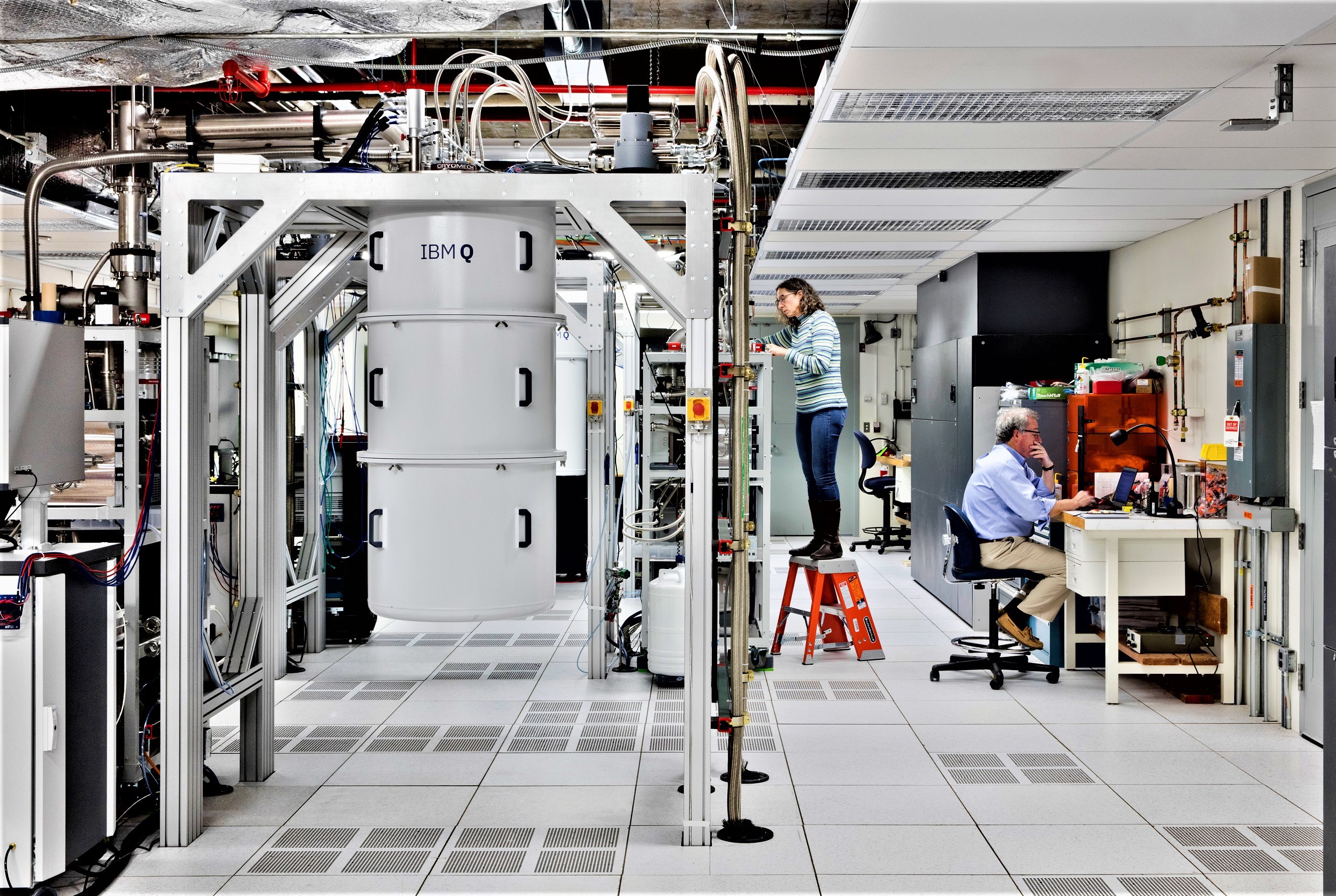
Figure 1.2: A research-grade superconducting quantum processor. The processor is located inside the white dilution refrigerator hanging from the support structure. The refrigerator cools the processor to the milliKelvin temperatures required to operate it;Source:IBM

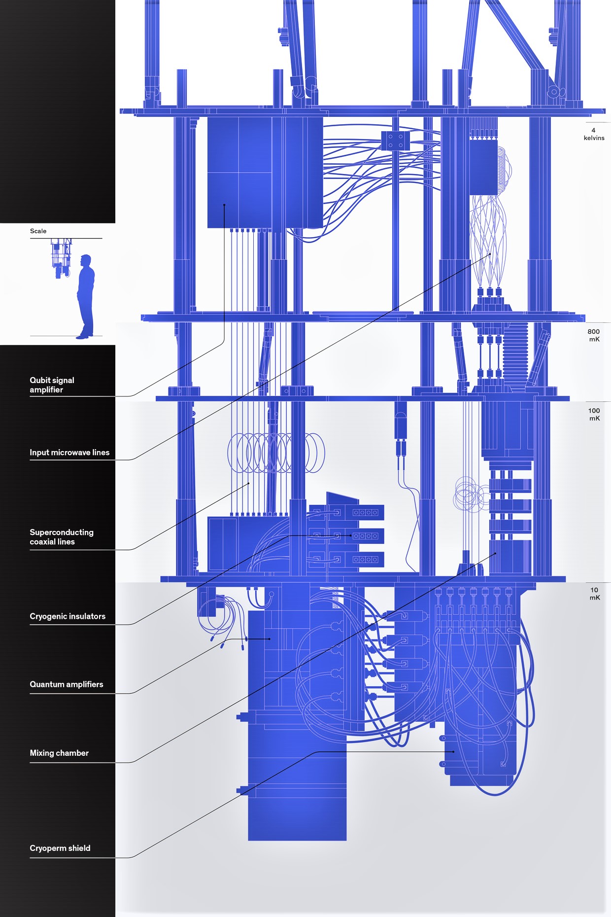
Figure 1.3: Dilution refrigerator;Source:IBM

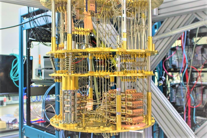
Figure 1.4: superconducting quantum processor;Source:IBM

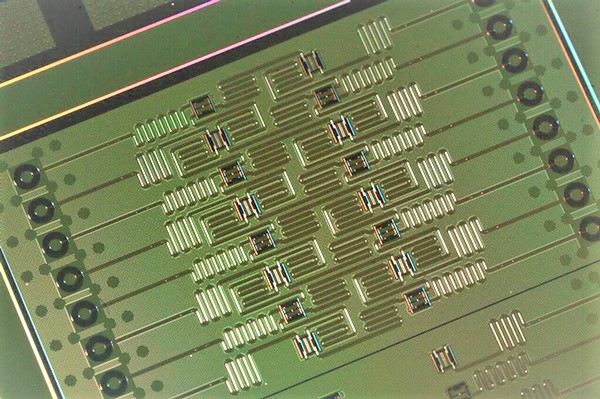
Figure 1.5: superconducting qubit citcuit;Source:IBM

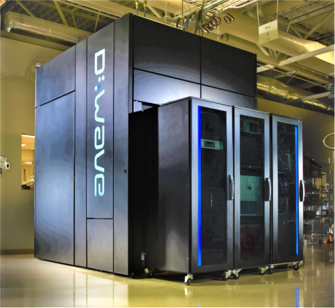
Figure 1.6: superconducting quantum annealer;Source:D-Wave

In the picture above, we see a large research-grade “dilution refrigerator” used to house and cool a prototype superconducting quantum processor. Refrigeration is required to cool the quantum chip to its operating temperature of less than 20 milliKelvin, a temperature more than 100 times colder than outer space. The refrigerator also serves to reduce the thermal load and noise that would otherwise degrade performance, arising in large part from the room-temperature electronics connected to the chip through various types of electrical cabling. To the left of the refrigerator are racks of such electronics, including arbitrary waveform generators, microwave signal generators, and current sources used to control the processor.

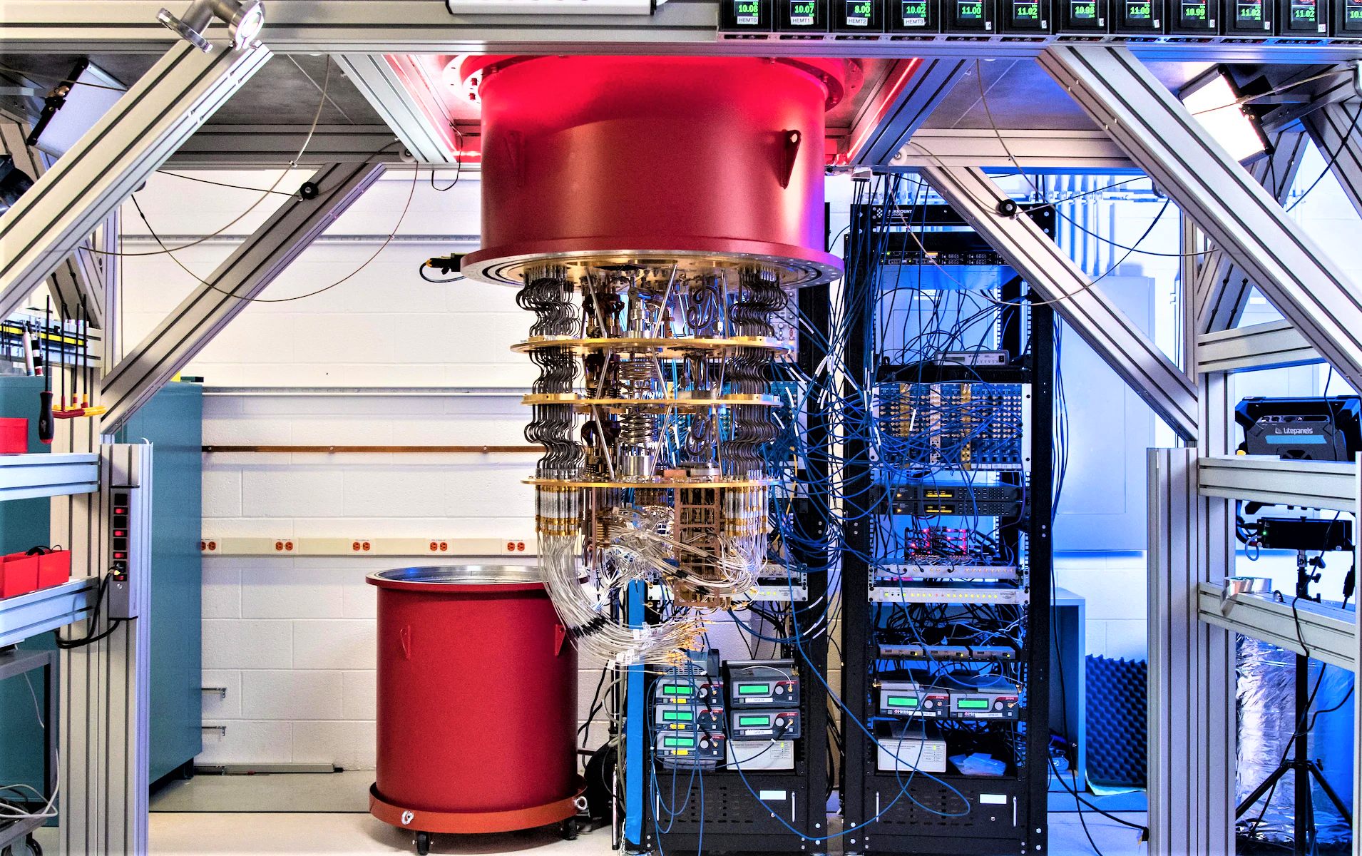
Figure 1.7: Google System;Source:Google

Figure 1.8: Google superconducting quantum processor;Source:Google

In the figure below, we see an optical table, on which stands a large black box housing the optical system used to control and measure a trapped-ion quantum computer[53]. The trapped ion computer “core” itself may reside in a cryogenic chamber at a temperature around 3-4 Kelvin, a temperature similar to outer space to obtain and maintain an ultra-high vacuum (although this is not required). High-stability lasers send light through a variety of mirrors, beamsplitters, optical modulators, and the like to address and read the individual ions that comprise the quantum computer.

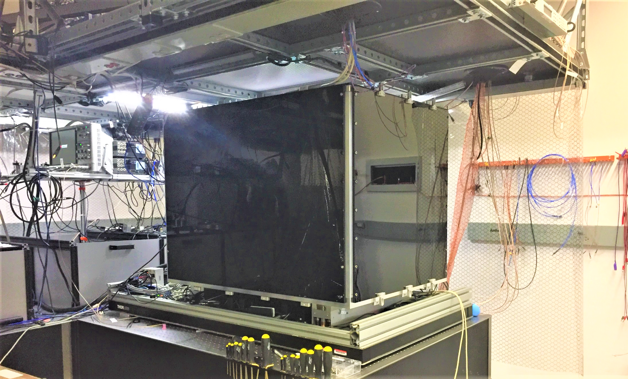
Figure 1.9: Trapped-ion quantum computer; Source: IonQ

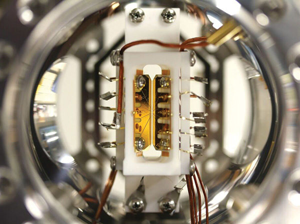
Figure 1.10: Trapped-ion quantum computer; Source: Joint Quantum Institute

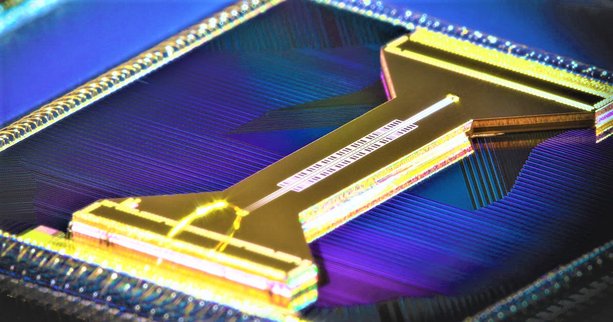
Figure 1.11: Honeywell’s Ion Trap Quantum; Source: Honeywell

Figure 1.12: Trapped ion quantum computer; Source: NIST

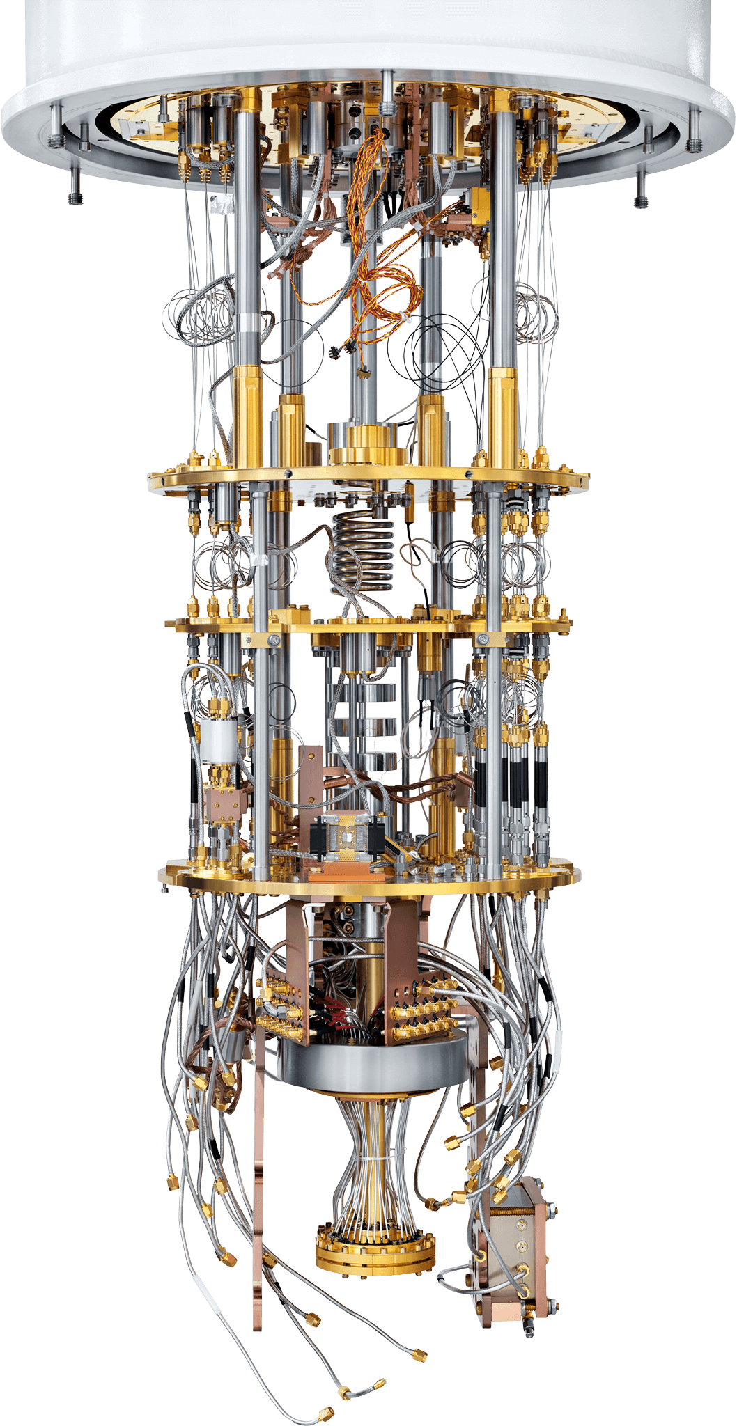
Figure 1.13: QPU (quantum processing unit) ; Source: Rigetti

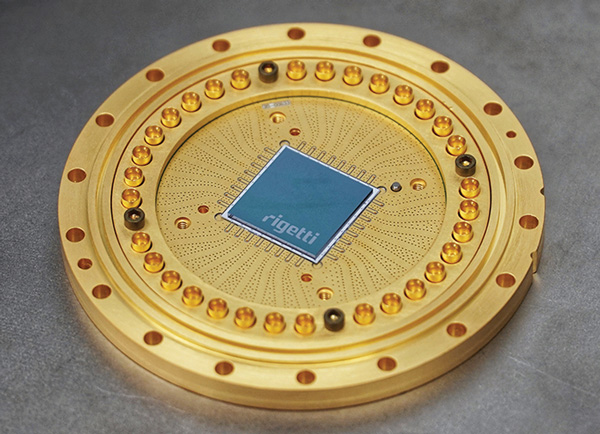
Figure 1.14: gold-plated copper disk with a silicon chip; Source: Rigetti

Figure 1.15: 49 qubits superconducting quantum processor Tangle Lake; Source: Intel

1.4   Physical and Conceptual Models of Classical Computation

To understand quantum computing, we first need to understand how information is processed today and, more generally, what constitutes “a computer” and “computation.”
The most common approach to classical information processing today uses a conventional electronic computer comprising a memory and a transistor-based computational processing unit. However, this is not the only physical manifestation of a classical computer. For example, human beings and our brains process information with different physical methods and architectures [54]. As these two examples suggest, there are many physical models of classical computation.
Physical Models of Classical Computation:
Mechanical: A computational system built with primarily mechanical components is a mechanical computer. Adding machines used for bookkeeping during the first part of the last century is an example of such computers. The input system is composed of numbered key buttons. After entering the numbers, a user pulls the crank, gear-wheels start turning, and the sum is mechanically computed and displayed. As in the case of an adding machine, mechanical computers are generally designed to implement application-specific tasks.
Electrical: Electrical computers use electrical elements that switch on/off electrical currents or voltages. Today’s personal computers are in this class, and they use transistors as the fundamental switching elements. Transistors enable the construction of a universal classical computer, one that can, in principle, tackle any computable problem. However, it may not be able to do so efficiently (in a reasonable amount of time or using a reasonable amount of physical hardware).
Optical: Systems that use photons the fundamental particles of light to perform computation are optical computers. The gates used to perform logic with photons can be engineered using nonlinear optical materials. As of today, existing optical computers tend to be application-specific.
Biological: Biological molecules, for example, proteins or DNA, can be used to process information. The individual, necessary elements for a fully operational biological computer, such as biological transistors, have been demonstrated. However, present biological, computational systems are hybrids that require the addition of electrical or mechanical components to operate.
There are also several conceptual models and architectures of classical computation, which in principle, any of the above physical systems can be used to process information.
Conceptual Models and Architectures of Classical Computation:
Turing Machine: A Turing machine comprises a memory tape and reads/write head. The memory tape is divided into discrete cells that store data. The head successively manipulates the cells. According to a set of rules, cell data may be altered depending on the cell’s prior information, which is also accessible by the head. This scheme provides an architecture to construct universal computational systems.
Cellular Automaton: A cellular automaton comprises an array of cells, each connected to several of its neighboring cells. After the cells are set to initial values, the cellular automaton evolves according to a set of rules that governs how the state of each cell changes in response to the states of its neighboring cells. Depending on the rules and connectivity of the cells, the result may be a uniform, oscillating, chaotic, or another intricate pattern. This computational concept is used to simulate or mimic the behavior of biological or chemical systems. For example, a global function emerges from a large number of seeming independent agents that interact with one another in a specified way.
Von Neumann Architecture: Architectures comprising a central processing unit and a memory unit are called von Neumann architectures. The central processing unit contains a controller, an arithmetic logic unit, and registers. The controller manages the computational processes: it requests data from memory, stores it in a register, directs the arithmetic logic unit to process the data in the register, and then sends the result back to the memory. This model is used for most present-day computational devices.

We are all familiar with laptop computers, desktop computers, even servers in the cloud that we interact with daily. In this section, we will refer to these as classical computers to contrast them with quantum computers. We will be discussing in detail later in the section. Classical computers use transistor-based integrated circuits-computer chips to process information and solve problems, whether for implementing a financial transaction, simulating a weather pattern, developing a CAD design, or even just drafting an email to a colleague. However, it is important to remember that there are many alternative ways in which one can process information. So, before we get started, let us discuss about what constitutes a computer and computation. There are many models of classical computation, and we would like to illustrate a wide variety of models, some of which we might find unexpected. One model is mechanical. So, for example, the thermostats on the walls, are driven by pneumatic pressure, and they actuate a little switch. So, they are a little kind of computer that controls temperature, but it is an analog computer. So mechanical computers do not need to be digital. They can come in all kinds of shapes and forms. the one that is the most famous in history is Babbage’s difference engine. We can have electrical circuits, which are ways of building a universal classical computer. We can also have optical computers that are made from information carriers that are photons and not electrons. Biological. In many ways, we and We are walking, discussing computers. this idea of biology and biological systems as computers is currently going through a renaissance because of the notions of neural networks [55, 56] and deep learning and these kinds of networks of neurons that act as computation. We also want to make a distinction between these models and some conceptual models. These are models by which we might realize computation, and these are the conceptual models that we might want to realize, one of them, the Turing machine. It is a machine that has a head and tape, and the tape has slots on it, which may have ones and zeros. it is something which has an extent to left and right, which goes off, in principle, to infinity. the tape is a kind of memory. the thing which is ostensibly doing the computation is a head that can read and write to this tape, but the only thing inside this head is a finite state machine. So, there are different states, and there are transitions between the states which happen to depend on what is read at what time and the earlier state that it used to exist. Turing machines like this come in many different flavors. There are probabilistic Turing machines, and there are universal Turing machines. So, given a certain kind of structure of a finite state machine here, we find that this Turing machine, then, can simulate any other Turing machine. Here are another model cellular automata. here, the model of computation is a world which is a grid in two dimensions in n dimensions where the point is that we have some kind of state in a local cell of this grid, and it undergoes transitions based on the state of its neighbors. we may have a local Cartesian neighborhood. we may have super Cartesian, but depending on what we are surrounded by, we change our state. we change ourselves to become empty or filled or different colors and so forth. these rules of patterns and pattern changes can give rise to computation. There is Von Neumann architecture. It is, again, a conceptual model of computation. here, the idea is to split memory from something which does arithmetic. So, we have an arithmetic logic unit, for example, some registers. Memory reads out data and feeds it into this ALU. Then the ALU feeds data back into the memory, and this is the model that is used by all processors today, including the ones on all our phones. There is DNA-based computation. This is the idea that we have strands of bases in AGCT, and then, A and T associate each other, which is called ligation. then G and C also ligate together. when we have two different strands of DNA, they will pattern match other strands in the right locations to produce base-pair ligations. this has been shown to allow a kind of computation using polymerase chain reaction tools. If we have a beaker, for example, with just one DNA strand, with PCR, we can amplify the number of DNA strands there so we can detect a certain DNA sequence. Thus, it is elegant that we can think of using such tools to do computation. we want us to be open to such models of computation, especially today, because we are starting to reconsider what it means to do computation. In many ways, we are at the end of the road of silicon today. We cannot rely on Moore’s Law much longer to provide increasing scaling. That is exponential of capability and size, power, and weight to build the computers. We need to look at different physical mechanisms to build computation. that is why all these different approaches, where we represent information in different ways, is so appealing to think about because the next thing beyond silicon, could be something different very different that utilize these ideas. we might discover that it is already happening all around us, or within us, if we only know how to think about it in the right way. So, although this section is about quantum computation, ostensibly, what We want to think about is how we are also thinking about a broader question of what is the physics of computation? How do we think of physical mechanisms as doing computation? Moreover, how do we think we might be able to exploit physical mechanisms and biological mechanisms that exist to realize the computations that we want to achieve?

1.5   Origins of Quantum Computing

How long has the idea of quantum computing been around? When did it start, and what have been the key milestones in its development? Before answering these questions for quantum computing, it is worth looking back at the history of classical electronic computing and how those technologies developed over the past 100 years.

The development of classical computers did not jump directly from the vacuum tube to laptops and smartphones. Commercial demand for intermediate products throughout the 1900s incentivized companies to develop and advance the technologies that, over time, led to the ubiquitous classical computers we have today. Early examples of such “off-ramp” products include:

Radar: Before being replaced by transistors, vacuum tubes were used to modulate radar signals.

Frequency mixers: Some of the first research on transistors developed out of an attempt to build frequency mixers for radio receivers during World War II. It was the starting point for Bell Lab’s work on transistors.

Transistor radios: The development of the bipolar junction transistor lead to the creation of transistor radios sold by companies like Texas Instruments, IDEA, and Sony. Unlike vacuum-tube radios, which could not output sound while the tubes were warming up, transistor radios could turn on and output sound immediately.

Amplifiers: Transistors were used (and are still used today) in all manner of products requiring electrical amplification, including sound speakers, hearing aids, radios, and telephones.

Along these lines, it will be challenging to sustain intense commercial interest and funding for quantum computing technology development if the first useful quantum computer is a 1,000,000-qubit fault-tolerant machine that is still 20-30 years in the future. Nearer-term commercial applications of quantum information [1] technologies will be needed to seed and maintain the virtuous cycle of technology development needed to realize large-scale quantum computers. Some of these quantum information technologies “off-ramp” applications could be, for example,

Noisy, intermediate-scale quantum simulation: Small, error-prone quantum computers may find use in simulating small-scale quantum systems perhaps as a co-processor to a classical computer.

Noisy, intermediate-scale Optimization: Noisy, error-prone quantum computers may also have applications to optimization or classification problems. For more examples of noisy, intermediate-scale quantum (NISQ) applications of quantum computing [28].

Besides, the various components needed to build these quantum systems will likely generate new business opportunities and expand existing ones. For example, the optics, electronics, refrigeration, software, and services are likely “ dual-use” beyond solely quantum computing. These products will benefit from the enhancements required for quantum computing and, in this enhanced state, support customers with applications beyond solely quantum computing.

Before diving into quantum computing, revisiting the history of classical electronic computing in the last century is worthwhile. We will see a few takeaways from this history that are relevant to the current and future development of quantum computing. Lee De Forest invented the first three-terminal triode vacuum tube in 1906. Vacuum tubes, much like the transistors that would later follow, are essentially faucets for electricity. The application of a small voltage on one terminal effectively opens a valve, which allows current to flow between the other two terminals. As such, vacuum tubes were used primarily as amplifiers for radio receivers, but they could also be used as on/off switches to implement logic gates. Thus, it was about 40 years after that first invention. We had the first large scale computers based on vacuum tubes, such as the electronic numerical integrator and the computer, or ENIAC, developed at the University of Pennsylvania in the 1940s. Also, around that time in 1947, the first transistor was invented at Bell Laboratories, and the first fully transistor-based computer soon followed. That computer, the transistor experimental computer number 0, or TX0, was built at MIT and Lincoln Laboratory in the mid-1950s, and it featured discrete transistors and magnetic core memory. Quite different from the computers we know and use today. Shortly after that, in 1959, the first integrated circuits using silicon were demonstrated. However, still, it was a good 20 or 30 years before we had the types of integrated circuit chips and memory chips that we now use in the computers daily. The first commercially available monolithic processor, the Intel 4004, appeared in 1971. It was a 4-bit processor, featured 2100 transistors, and clocked in at around 740 kilohertz. Within a year or two, however, Intel came out with another processor, the 8008. An 8-bit processor with nearly double the number of transistors. This doubling of the number of transistors approximately every two years was exemplary of what became known as Moore’s Law. by the 1990s, following Moore’s Law, the number of transistors had increased into the millions. today, we have computer chips with five billion transistors or more with multicore processors and graphical processing units, GPUs with close to 20 billion transistors. Although performance increases had previously simply followed from this Moore’s law type scaling, these straightforward improvements have significantly waned over the past decade. Nonetheless, with the development of high k dielectrics, low resistance interconnects, multicore processors, 3D integration, and the like, we can expect continued improvements in the performance of classical processors for years to come. In contrast to these 100 plus years of classical computing development, quantum computing is much more recent. In the early 1980s, Richard Feynman suggested that if we want to simulate a quantum system, a task that is very hard for a classical computer, we should use a quantum system to perform that simulation [57, 58]. He was suggesting we should build a quantum computer. He also noted that it is a fascinating problem, because it is not so easy, and he was right. Over the next decade or so, researchers thought about what kinds of algorithms could potentially give a quantum advantage for real-world problems of significance, and how fragile quantum states could ever be used to implement such an algorithm. The answers started in the mid-1990s, including two significant milestones in the history of quantum computing. The first was the discovery of Shor’s algorithm, developed by Peter Shor [59]. Shor’s algorithm was not the first quantum algorithm to show the quantum advantage. However, it was the first that also addressed an important practical problem, namely the factorization of large numbers. Now that is an important problem because the difficulty of factorization is a pillar for the present-day encryption schemes that protect the information. Essentially factoring large numbers is a very challenging problem on a classical computer, which is why it is used for public-key encryption. Peter Shor showed that factorization could be done efficiently on a quantum computer. Also, around that time, Peter Shor and his colleagues Robert Calder bank and Andrew Steane developed the first quantum error-correcting codes [60], which, once fully implemented, will enable quantum computers to continue to operate robustly in the presence of errors. Since then, researchers have focused on both the underlying physics, as well as the hardware that we can use to build quantum computers. Starting at the single-qubit level, researchers have explored numerous qubit modalities, from superconductors to trapped ions, semiconductors, and more. Today we have processors operating with 10 to 20 qubits and reports of 50 qubits being available soon. There is also a marked transition from prototype demonstrations in the early 2000s to where we are today, which is engineering larger and larger quantum systems. We are even now seeing examples of cloud quantum computers [61] on the web that can be used by people worldwide to try out algorithms, and We will use one in this section. So, what does this all mean? Well, we think there are a couple of takeaways from this brief historical discussion. The first is that technology development takes time. It took over a century to get from the first triode vacuum tubes to the computers we have today. That development is not over. It continues today. there are many changes along the way. The right approach to building a classical computer changed many times over the years. There was no single right answer. The right technology in the 1940s was different from the 1980s, and that was also different from today. Nonetheless, in hindsight, all these steps were crucial to the overall development. Similarly, we can expect that going forward, and quantum computing will likely go through technology evolution. The best qubit modalities today are not necessarily the ones that will excel in the future. However, the observation is that in the absence of effort, we should not expect the right technology to appear if we wait long enough. Technology is developed; it is not bestowed. The road to future quantum computers, whatever they may end up looking like, is paved with the technologies we develop today. Finally, we should not underestimate the crucial role that commercialization played in the development of classical computing technologies. From the very beginning, transistors had commercial applications that generated revenue long before computers were available, including radio amplifiers, hearing aids. Although governments played a key role in seeding the development of transistor-based computers and are playing an equally crucial role in the development of quantum computers today, it was commercial development of transistors and computer chips that ultimately enabled the virtuous cycle of development that made possible Moore’s law like scaling that led to the computers we use today. a major challenge for quantum computing is to identify these kinds of commercially useful applications. For qubits and small-scale quantum processors that can kickstart a similar virtuous development cycle. One that will be needed if we are to realize large scale quantum computers.

1.6   How is a Quantum Computer Different

How is a quantum computer different than a classical computer? In this section, we will compare and contrast classical and quantum computers to gain a better understanding of the unique ways in which a quantum computer represents information.

So how is a quantum computer different? We can begin to answer that question by comparing it with a classical computer. Classical computers are the computing devices that we use every day at work and home, and they process information using transistors, each of which can store one bit of information. We will call this a classical bit, which is binary, and it can take on one of two states. It can either be in state 0, let us say the absence of a voltage on the transistor gate, or it can be in state 1, the presence of a voltage on that gate. These are discrete, robust states, and when we measure the state of that transistor, we will see either a 0 or a 1, depending on where that bit was set. We can contrast that with a quantum computer, which is built from logical elements called qubits, which is short for quantum bits. A qubit is binary in the sense that it is realized using a quantum coherent two-state system, and so it can be set in state 0 or state 1, but because it is quantum mechanical, it can do much more. A qubit can also be at a quantum superposition state. It is a single state, but it carries aspects of both state 0 and state 1 simultaneously, and this is a manifestly quantum mechanical effect. We can represent a qubit state on what called a Bloch Sphere, which for this discussion, we can think of as the planet Earth, where state 0 is at the North Pole, and state 1 is at the South Pole. In this representation, a classical bit can be either at the North Pole or the South Pole, but that is it.

Figure 1.16: The two logical states of a classical system correspond to north and south on a globe

In contrast, a qubit can exist anywhere on its surface. Now, a qubit can also be at the North Pole or the South Pole. That is fine, but when it is anywhere else, the qubit is in a superposition state, again, a single state that takes on aspects of state 0 and state 1 simultaneously, as shown in the notation here. Superposition states result in probabilistic measurements, meaning that if we had said an equal superposition of 0 and 1, and we measure the qubit, we have a 50/50 chance of measuring in state 0 and a 50/50 chance of getting state 1. If we identically prepare that same state and measure it, and do that repeatedly, Half of the time, we will get a 0, and Half of the time, and We will get a 1. As a result, quantum computers rely on encoding information in fundamentally different ways than classical computers. So, on a classical computer N, classical bits represent a single N-bit state. For example, if N equals 3, we have 3 classical bits, and they can represent the state 000 or 001, all the way up to 111. There are eight different combinations, but the three classical bits can represent only one of them at a time. Thus, when we want to process the information on a classical computer, we pick one of those states as the input, we process the information, and we get a result as an output. However, if we also want to process information using a different input state, we have two choices. We can either process in parallel by using additional copies of the hardware, or with added time, we can process sequentially on the same piece of hardware. It is classical parallelism, and in both cases, we needed more resources, either more hardware or more time. The qubits in a quantum computer, on the other hand, can be set into a single superposition state that simultaneously carries aspects of all these 2 to the N components. So, for example, with three qubits, a quantum computer can represent aspects of all eight different components in a single quantum superposition state. Consequently, we have a quantum version of parallelism, and importantly, we also have quantum interference between those constituent components. Quantum parallelism and quantum interference make a quantum computer different, and in the next section, we will give examples of how they work in a quantum processor.

In transistor-based classical computers, a transistor represents a classical binary bit that can store one bit of information. In one of two distinct logical states, classical bits are found in logic state 0 or logic state 1. “State 0” corresponds to the transistor switch being “off” (e.g., no voltage is applied to the transistor gate, and so no current flows in the transistor channel), and “state 1” corresponds to the transistor switch being “on” (e.g., a voltage is applied to the gate, and so a current flows through the transistor channel). These discrete states are robust and can be measured with near certainty.

The fundamental elements of quantum computers are “quantum bits”, typically referred to as “qubits.” Qubits are quantum-mechanical two-level systems. They are binary in the sense that they can be initialized in classical states 0 or 1. However, as quantum mechanical objects, qubits can also be prepared in a quantum superposition state: a single quantum state that embodies aspects of both state 0 and state 1.

Quantum superposition states are succinctly represented using Dirac notation [62, 63, 64, 65, 66, 67]. In this notation, quantum states are expressed as “kets,” where $|0\rangle$ and $|1\rangle$ represent the quantum states 0 and 1 respectively. A qubit that is in a superposition of these two states is then written as $|\psi\rangle=a|0\rangle+b|1\rangle$. The coefficients a and b are called “probability amplitudes,” and they are related to the relative “weighting” of the two states in the superposition. An obvious special case occurs when either is zero, in which case the state$|\psi\rangle$ is no longer in a superposition. For example, if $a=0$, then $|\psi\rangle=|1\rangle$. More generally, both a and b can be complex numbers and therefore must satisfy $|a|^{2}+|b|^{2}=1$, a normalization to unity that ensures the “weights” being compared are of a standard, consistent size. This is analogous to the convention that probabilities are set to sum to 1.

Both classical and quantum bits can be visualized on a “Bloch sphere,” a tool which can be thought of as the planet Earth, as pictured in Fig. 5. By convention, the “north pole” of the sphere represents state 0, and the “south pole” represents state 1. A classical bit is either at the north pole or the south pole, but nowhere else. In contrast, a qubit may exist anywhere on the surface of the sphere. When the qubit state is anywhere except for the north and south poles, it is in a superposition state.

Figure 1.17: The Bloch Sphere

To better illuminate the connection between the state of a qubit and the Bloch sphere, the coefficients of the state $|\psi\rangle$ can be expressed as $|\psi\rangle=\cos\left(\theta/2\right)|0\rangle+e^{i\phi}\sin\left(\theta/2\right)|1\rangle$. It is a straightforward exercise to confirm that these coefficients satisfy the normalization condition mentioned above. The two angles $\theta$ and $\phi$, determine the point on the surface of the Bloch sphere corresponding to the state $|\psi\rangle$, as pictured in Fig. 6. Intuitively, these angles relate to the globe in Fig. 5, because $\theta$ moves the state $|\psi\rangle$ in the north-south direction and corresponds to the qubit “latitude,” while $\phi$ moves the state along the east-west direction and corresponds to its “longitude.”

Ideal projective measurement of a qubit occurs along a single axis of the Bloch sphere, for example, the z-axis (which on the globe would be the line connecting the north and south poles). It is called the measurement basis, and measurement will yield a classical result either “state 0” or “state 1” along this axis. The measurement process itself is probabilistic, and the probability of obtaining either $|0\rangle$ or $|1\rangle$ is related to the qubit’s projection onto the measurement basis. As an example, consider when the qubit is an equal superposition of states $|0\rangle$ and$|1\rangle$. It occurs whenever $\theta=\pi/2$ and corresponds to the states along the equator of the globe. In these cases, the state, when measured along the z-axis, is equally likely to result in the outcome $|0\rangle$ or $|1\rangle$, because their probability amplitudes are the same. Intuitively, any point on the equator when projected onto the z-axis is at the center of the Earth, equally “far” from the north and south pole.

As a result, quantum computers rely on encoding information in fundamentally different ways than classical computers[68]. For N bits, there are $2^{N}$ possible classical states. However, a classical computer can represent only one of these N-bit states at a time. Processing multiple N-bit states can either be performed sequentially in time or parallel using additional copies of the hardware. It is classical parallelism. In contrast, the qubits in a quantum computer can be set into a single superposition state that may simultaneously carry aspects of all $2^{N}$ components. As we will see shortly, this enables two uniquely quantum mechanical effects: quantum parallelism and quantum interference.

In the context of the Bloch sphere, we have discussed about making measurements along what we call the qubits quantization axis, or the z-axis. the question was, basically, are there ways in which we can make measurements along different axes of the Bloch sphere? And the answer is yes. it depends a bit on the modality that we are discussing about. But generally speaking, we could always keep our measurement apparatus measuring along the z-axis. right before we make that measurement for example, if we wanted to measure the x-axis what we could do is a rotation that basically brings the x-axis to the z-axis and then make our measurement. so, we are still measuring along the z-axis. But by doing this rotation right before the measurement, we are effectively rotating the qubit states along x up to the z-axis and then making a measurement. so, this is a common way to do state tomography [69] and process tomography measurements when It is more convenient to just have our measurement basis be just along the x-axis, just along the z-axis is to do a rotation right before measurement to measure effectively in these different bases.

Bloch Sphere, The same way that a person’s position can be defined by a point on the Earth, a quantum state can be defined by a point on the Bloch sphere. While a point on the globe always refers to position, a point on the Bloch sphere refers to a qubit’s state. For example, a qubit state can be spin-up (north pole), spin-down (south pole), or in a superposition of spin-up and spin-down (anywhere else). Identify the qubit states on the Bloch sphere.

Figure 1.18: Bloch Sphere

On the Bloch Sphere, the z-axis runs from the south to the north pole of the sphere. Axes x-axis and y-axis are perpendicular to one another in the plane of the equator of the sphere. The north pole corresponds to state 0 (orange vector), and the south pole corresponds to state 1 (blue vector). The equator corresponds to equal superposition states. $(|0>+|1>)/\sqrt{(}2)$ is at the surface of the sphere in the +x direction. $(|0>-|1>)/\sqrt{(}2)$ is at the surface of the sphere in the -x-direction.

1.7   Dirac Notation

We discussed that a quantum bit qubit for short is the name given to a quantum-mechanical two-level system. The particular physical system we viewed was the spin of an electron in an atom, where the two states were spin-up and spin-down. Although qubits are realized using physical systems, it is advantageous to think of them as mathematical objects [70], because it will be easier to work with them using mathematics [71]. The approach is technology agnostic, independent of a particular physical system. In this unit, we will discuss basic concepts from linear algebra, necessary for understanding how quantum states and gates operate using Dirac notation[62, 63, 64, 65, 66, 67]. At the end of this unit, we will see the concept of measurement at a very high level; more details about it will be given in the following section.

As an introductory example, consider the state space representation of four light bulbs. In this classical system, each light bulb is a classical two-state system and can be either: OFF $\to$ state 0, or ON $\to$ state 1. It means that our classical system can be in $2^{4}=16$ possible configurations. Suppose that for some reason, we decide to communicate our ATM PIN (which is 1248) to our neighbor in an extremely insecure manner using light bulbs. To do this, we would first write each digit of the ATM number using binary representation, and then turn ON/OFF the lights according to the predefined state-space definition:

1=0001 $\to$ OFF OFF OFF ON,

2=0010 $\to$ OFF OFF ON OFF,

4=0100 $\to$ OFF ON OFF OFF,

8=1000 $\to$ ON OFF OFF OFF.

To send the decimal number 1, we will keep the first three bulbs OFF and the last one ON. To send the number 2, we will keep OFF the first 2 bulbs, ON the third bulb, and OFF the fourth bulb.

Quantum bits and classical bits both represent two-state systems, as in the section, qubits have unique quantum-mechanical properties. Thus, to represent the state of a qubit, people use a standard notation called Dirac notation, or “bra”-“ket” (read: bracket) notation. The representation uses vectors, which can then be manipulated using linear algebra concepts, such as matrix multiplication. If it has been a while, the following text and links will serve as a refresher.

1. States 0 and 1 are represented as kets $\left|0\right\rangle$ and $\left|1\right\rangle$ (the ket in bra-ket), and correspond to column vectors. In particular, ket $\left|0\right\rangle$ and ket$\left|1\right\rangle$ are usually written as:

$$\left|0\right\rangle=\left(\begin{array}[]{c}1\\ 0\end{array}\right)$$ (1.1)

$$\left|1\right\rangle=\left(\begin{array}[]{c}0\\ 1\end{array}\right)$$ (1.2)

2. Bras (the bra in bra-ket) are the Hermitian conjugate of kets. Operationally, a Hermitian conjugate is found by transposing a vector (or matrix) and taking the complex conjugate of each element. Since the states $|0\rangle$ and $|1\rangle$, as written above, contain only real numbers, the Hermitian conjugate is equivalent to the transpose and results in the following row vectors $\displaystyle\left\langle 0\right|\displaystyle=\displaystyle\left(\begin{array}[]{c c}1&0\end{array}\right),\displaystyle\left\langle 1\right|\displaystyle=\displaystyle\left(\begin{array}[]{c c}0&1\end{array}\right).$

The use of the Hermitian conjugate may be more evident after the next point.

3. The inner product between two states, say $\left|\phi\right\rangle$ and $\left|\psi\right\rangle$, is written as the bracket (as in, bra-ket) $\left\langle\phi\right|\left.\psi\right\rangle$, and in general results in a complex number. This is evident through an example. Consider the quantum state

$$\begin{split}\left|\psi\right\rangle&=\alpha|0\rangle+\beta|1\rangle\\ &=\alpha\left(\begin{array}[]{c}1\\ 0\end{array}\right)+\beta\left(\begin{array}[]{c}0\\ 1\end{array}\right)\\ &=\left(\begin{array}[]{c}\alpha\\ \beta\end{array}\right),\end{split}$$ (1.3)

3. Taking the inner product of two vectors shows that $\langle 0|\psi\rangle=\alpha$ and$\langle 1|\psi\rangle=\beta$. In this example, the inner product of the general state$|\psi\rangle$ with each of the basis states$|0\rangle$ and $|1\rangle$ returns a number which corresponds to the “probability amplitude” of $|\psi\rangle$ in each of those states. Hence, the Hermitian conjugate is a mathematical tool used to calculate the projection of one state onto another. Finally, it should be noted that since the inner product is a complex number in general, it can be decomposed into a product of its modulus (it is magnitude) represented as $\left|\left\langle\psi\right|\left.\phi\right\rangle\right|$and a phase factor, $e^{i\theta}$, where $\theta$ is the angle between the vectors representing the states $\left|\psi\right\rangle$ and $\left|\phi\right\rangle$.

4. The norm or “length” of the vector representing a state $\left|\psi\right\rangle$ is given by the square root of the inner product:
$\left|\left\langle\psi\right|\left.\psi\right\rangle\right|=\sqrt{\left\langle\psi\right|\left.\psi\right\rangle}.\sqrt{\left\langle\psi\right|\left.\psi\right\rangle}$

5. Physical states represented in ket notation have a norm equal to one, that is $\left\langle\psi\right|\left.\psi\right\rangle=1$. Checking and ensuring that the norm of a state has unit value is procedure called “normalization”. Since $\left|0\right\rangle$ and $\left|1\right\rangle$ are physical states with unit norm, they must also satisfy the following condition (since $1^{2}=1)$:

$$\left|\left\langle 0\left|\right.0\right\rangle\right|=\sqrt{\left\langle 0\left|\right.0\right\rangle},\;\;\left|\left\langle 1\left|\right.1\right\rangle\right|=\sqrt{\left\langle 1\left|\right.1\right\rangle}.$$ (1.4)

States $\left|0\right\rangle$ and $\left|1\right\rangle$ are orthogonal, i.e $\left\langle 0\left|\right.1\right\rangle=\left\langle 1\left|\right.0\right\rangle=0.$ This means there is no projection of state $\left|0\right\rangle$ on to state $\left|1\right\rangle$ and visa versa. They are independent vectors, and so there is no way to write $\left|0\right\rangle$ in terms of $\left|1\right\rangle$ or vice versa; this is called linear independence.

When a quantum state is the sum of linearly independent states, such as $\left|0\right\rangle$ and $\left|1\right\rangle$, it is said to be in a superposition state. This is the case for the state $|\psi\rangle=\alpha|0\rangle+\beta|1\rangle$ defined above. The coefficients $\alpha$ and $\beta$ are referred to as probability amplitudes and, as we have discussed, are in general complex numbers. The hermitian conjugate of $\left|\psi\right\rangle$ is $\displaystyle\left\langle\psi\right|\displaystyle=\displaystyle\alpha^{*}\left\langle 0\right|+\beta^{*}\left\langle 1\right|,\displaystyle=\displaystyle\left(\begin{array}[]{c c}\alpha^{*}&\beta^{*}\end{array}\right)$, where $\alpha^{*}$ and $\beta^{*}$ are the complex conjugates of $\alpha$ and $\beta$ respectively.

To better understand the probability amplitudes $\alpha$ and $\beta$ of $|\psi\rangle$ represent, Let us think more about the superposition concept. A light bulb is either ON or OFF, and that is it. When we look at it, or “measure” it, we know precisely which state it had been in and continues to be in. On the other hand, while a quantum system can certainly be in the classical states $\left|0\right\rangle$ or $\left|1\right\rangle$, it can also be in a superposition state: a single state that carries aspects of both $\left|0\right\rangle$ and $\left|1\right\rangle$. What does this mean?

Let us take a qubit prepared in the superposition state $|\psi\rangle=\alpha\left|0\right\rangle+\beta\left|1\right\rangle$. When this qubit is measured, quantum mechanics tells us that the qubit state will be projected onto our measurement basis. In the examples in the section, we are measuring along the z-axis, that is, the axis which represents states $\left|0\right\rangle$ and $\left|1\right\rangle$. Measurements must give us a classical result, and so any given measurement will result in one of the classical states: either state $\left|0\right\rangle$ or state $\left|1\right\rangle$. We never measure a superposition state directly. However, if we identically prepare and measure the state $\left|\psi\right\rangle$ many times, we will find that we will obtain state $\left|0\right\rangle$ with probability $\left|\alpha\right|^{2}$ and state $\left|1\right\rangle$ with probability $\left|\beta\right|^{2}$. We call the coefficients $\alpha$ and $\beta$ probability amplitudes, since their magnitude squared will yield the probability that we measure their respective states. As shown in the example in (3) above, these probability amplitudes can be found by projecting the vector representing state $\left|\psi\right\rangle$ onto the vectors representing the states $\left|0\right\rangle$ and $\left|1\right\rangle$.

Figure 1.19: 0 and 1 states

This is represented in the last figure, which shows the projection of the superposition state $\left|\psi\right\rangle=\alpha\left|0\right\rangle+\beta\left|1\right\rangle$ on to the measurement axis corresponding to states $\left|0\right\rangle$ and $\left|1\right\rangle$. Notice that the closer the state $\left|\psi\right\rangle$ is to $\left|0\right\rangle$, the larger the projection $\left|\alpha\right|$ and thus the probability $\left|\alpha\right|^{2}$of measuring state$\left|0\right\rangle$. In fact, when $\left|\psi\right\rangle$ coincides with $\left|0\right\rangle$ the value of $\left|\alpha\right|$ becomes equal to 1, and we will measure state $\left|0\right\rangle$ with certainty (probability $\left|\alpha\right|^{2}$ equal to 1).

To summarize, a superposition state $\left|\psi\right\rangle=\alpha\left|0\right\rangle+\beta\left|1\right\rangle$ satisfies the normalization condition $\left|\alpha\right|^{2}+\left|\beta\right|^{2}=1$ (this ensures that the probabilities of measuring all states add to unity), and the probability of measuring the states $\left|0\right\rangle$ and $\left|1\right\rangle$ are $p(0)=\left|\left\langle 0\right|\left.\psi\right\rangle\right|^{2}=|\alpha|^{2}$and$p(1)=\left|\left\langle 1\right|\left.\psi\right\rangle\right|^{2}=|\beta|^{2}$ respectively.

1.8   Bloch Sphere

The Bloch sphere is a useful tool for visualizing single-qubit states. Using Dirac notation, as we have discussed, one can write an arbitrary single-qubit state $|\psi\rangle$ as

$$\lvert\psi\rangle=\alpha\lvert 0\rangle+\beta\lvert 1\rangle,$$ (1.5)

where $\alpha$ and $\beta$ are the probability amplitudes and $|\alpha|^{2}+|\beta|^{2}=1$. In general, probability amplitudes are complex numbers, and can therefore always be written as the product of a real number and a complex exponential phase factor. For example, the probability amplitudes $\alpha$ and $\beta$ can be expressed as

$$\alpha=|\alpha|(\cos\phi_{\alpha}+i\sin\phi_{\alpha})=|\alpha|e^{i\phi_{\alpha}}\rightarrow ae^{i\phi_{a}},$$ (1.6)

$$\beta=|\beta|(\cos\phi_{\beta}+i\sin\phi_{\beta})=|\beta|e^{i\phi_{\beta}}\rightarrow be^{i\phi_{b}},$$ (1.7)

where $a=|\alpha|$ and $b=|\beta|$ are the magnitudes of $\alpha$ and $\beta,$ and $\phi_{a}=\phi_{\alpha}=\arg(\alpha)$ and $\phi_{b}=\phi_{\beta}=\arg(\beta)$ are the arguments $\alpha$ and $\beta$ referred to as “phases”. Using this convention, the single-qubit state $|\psi\rangle$ becomes

$$\begin{split}\lvert\psi\rangle&=ae^{i\phi_{a}}|0\rangle+be^{i\phi_{b}}|1\rangle\\ &=e^{i\phi_{a}}\left(a|0\rangle+be^{i(\phi_{b}-\phi_{a})}|1\rangle\right)\\ &\equiv e^{i\phi_{a}}\left(a|0\rangle+be^{i\phi}|1\rangle\right)\end{split}$$ (1.8)

where we have factored out the phase $e^{i\phi_{a}}$, referred to as the global phase, and defined a relative phase $\phi=\phi_{b}-\phi_{a}$ with $\phi$ defined from 0 to $2\pi$.

We do this because it is only relative phases that play a role in quantum interference or the values of physical observables based on measurements. Any phases that sit out front may be omitted without harm.

To see this explicitly, remember that the probability of measuring the state $|\psi\rangle$ in another state $|\mu\rangle$ is given by $p(\mu)=|\langle\mu|\psi\rangle|^{2}$. Defining $|\mu\rangle=e^{i\phi_{g}}\left(c|0\rangle+de^{i\phi_{r}}|1\rangle\right)$, a straight forward calculation yields:

$$\begin{split}p(\mu)&=|\langle\mu|\psi\rangle|^{2}\\ &=\left|\left(e^{-i\phi_{g}}\left(c\langle 0|+de^{-i\phi_{r}}\langle 1|\right)\right)\left(e^{i\phi_{a}}\left(a\lvert 0\rangle+be^{i\phi}\lvert 1\rangle\right)\right)\right|^{2}\\ &=\left|e^{i(\phi_{a}-\phi_{g})}\left(c\langle 0|+de^{-i\phi_{r}}\langle 1|\right)\left(a\lvert 0\rangle+be^{i\phi}\lvert 1\rangle\right)\right|^{2}\\ &=\left|e^{i(\phi_{a}-\phi_{g})}\left(ac+bde^{i(\phi-\phi_{r})}\right)\right|^{2}\\ &=\left|e^{i(\phi_{a}-\phi_{g})}\right|^{2}\left|\left(ac+bde^{i(\phi-\phi_{r})}\right)\right|^{2}\\ &=\left|\left(ac+bde^{i(\phi-\phi_{r})}\right)\right|^{2}.\\ \end{split}$$ (1.9)

Two important properties of complex numbers are used in this calculation. First, for any two complex numbers w and z, it is always true that $(wz)^{*}=w^{*}z^{*}$. And, second, $|z|^{2}=z^{*}z$ where $*$ denotes the complex conjugate. The latter property is useful because it means that $|e^{ix}|^{2}=e^{-ix}e^{ix}=1$ for any real x, and this leads to the removal of the global phases when calculating the measurement probability. This absence of both $\phi_{a}$ and $\phi_{g}$ from the final result, regardless of their value, indicates that the global phase has no physical relevance. Therefore, it is conventional to omit these phase factors from calculations.

Removing the global phase from $|\psi\rangle$reduces the number of variables needed to specify a state from four $(a,b,\phi_{a},\phi_{b})$to three $(a,b,\phi)$. One further degree of freedom can be removed by directly incorporating the normalization condition $\lvert\alpha\rvert^{2}+\lvert\beta\rvert^{2}=1$into the coefficients. Following convention, this is performed by parameterizing a and b using the trigonometric functions

$$\begin{split}a&=\cos\left(\theta/2\right),\\ b&=\sin\left(\theta/2\right),\end{split}$$ (1.10)

where $\theta$ goes from $0$ to $\pi$. The reason for selecting trigonometric functions is due to the natural geometric interpretation of the angle $\theta$, as will be discussed in more detail below. Therefore, the state of a single qubit can be represented in complete generality by

$$\lvert\psi\rangle=\cos\left(\theta/2\right)|0\rangle+\sin\left(\theta/2\right)e^{i\phi}|1\rangle$$ (1.11)

which has only two free variables.

Geometrically, $\theta$ and $\phi$ can be mapped to a point on a sphere, referred to as the “Bloch sphere”, using a spherical coordinate system. The angle $\theta$ is called the “polar angle”, and it is measured from the positive z-axis to the Bloch vector representing the state $\lvert\psi\rangle$. The angle $\phi$ is called the “azimuthal angle,” It is measured from the positive x-axis to the projection of state $\lvert\psi\rangle$ onto the x-y plane (see the figure for the correct orientation).
Let us consider the polar and azimuthal angles for a few standard quantum states.
First, Let us consider the “poles” where the z axis meets the surface of the sphere, corresponding to $\theta=0$ and $\theta=\pi$ and representing the states $\lvert\psi\rangle=|0\rangle$ and $\lvert\psi\rangle=|1\rangle$ respectively. Note that for $\theta=\pi,$ corresponding to $\lvert\psi\rangle=e^{i\phi}\lvert 1\rangle\rightarrow\lvert 1\rangle$, the angle $\phi$ becomes a global phase factor and is therefore not needed.
$-(\theta=0,\phi)\rightarrow|0\rangle$: this is the point where the z axis meets the north pole in the positive-z direction $(z=+1)$.
$-(\theta=\pi,\phi)\rightarrow|1\rangle:$ this is the point where the z axis meets the south pole in the negative-z direction $(z=-1)$.
Next, Let us consider the equal superposition states $\lvert\psi\rangle=|0\rangle+e^{i\phi}|1\rangle$ on the “equator” in the x-y plane. These states all share $\theta=\pi/2$, and are uniquely identified on the equator by the angle $\phi$. Let us further look at four specific examples as we work our way around the equator:
$-(\theta=\pi/2,\phi=0)\rightarrow\frac{1}{\sqrt{2}}\left(|0\rangle+|1\rangle\right):$ this is the point where the x axis meets the equator in the positive-x direction $(x=+1)$.
$-(\theta=\pi/2,\phi=\pi/2)\rightarrow\frac{1}{\sqrt{2}}\left(|0\rangle+i|1\rangle\right):$ this is the point where the y axis meets the equator in the positive-y direction $(y=+1)$.
$-(\theta=\pi/2,\phi=\pi)\rightarrow\frac{1}{\sqrt{2}}\left(|0\rangle-|1\rangle\right):$ this is the point where the x axis meets the equator in the negative-x direction $(x=-1)$.
$-(\theta=\pi/2,\phi=3\pi/2)\rightarrow\frac{1}{\sqrt{2}}\left(|0\rangle-i|1\rangle\right):$ this is the point where the y axis meets the equator in the negative-y direction $(y=-1)$.

Figure 1.20: Bloch Sphere

1.9   Quantum Parallel and Interference

How does a quantum computer process information? How can quantum logic operations lead to quantum advantage? In this section, we will be introduced to two quantum-mechanical phenomena quantum parallelism and quantum interference that are fundamental to quantum information processing [1, 72, 73]. We will be given visceral, intuitive examples that allow us to “see” directly how the quantum versions of parallelism and interference efficiently manipulate the weighting coefficients probability amplitudes within a quantum superposition state, process quantum information.

Quantum parallelism and quantum interference are what make a quantum computer different than a classical computer. However, what is these quantum effects? Furthermore, how do they work in a quantum computer? To gain some insight, we will consider an example of a small quantum computer with three qubits. Here we have three atoms. Each of which has an electron with a spin. Moreover, each of these spins can either be pointed up, which We will call spin-up, or pointed down, which We will call spin-down. We will use these three electron spins as the qubits. There are eight different spin combinations that we can have, from all three pointed up, to all three pointed down. We place these qubits in a single quantum superposition state, comprising all eight of these spin configurations. It takes eight complex numbers, C1 through C8, to specify the weighting of each of these components. The superposition state can then be represented as a state register with all eight spin configurations and their respective coefficients. Let us now imagine that we want to perform an operation that flips the spin of Atom 1. We can do this by applying an electromagnetic pulse with the right strength and the right duration, such that it rotates the spin of Atom 1 by 180 degrees. It is called a $\pi$ pulse. Furthermore, it acts to flip the spin. Spin-up rotates to spin-down, and spin-down rotates to spin-up. So, when we flip the spin in Atom 1, it acts to flip the spin on each of the spins in the configurations that make up the superposition state. For example, the coefficients C1 through C4, associated initially with spin-up in Atom 1, are now associated with spin-down. Similarly, the coefficients C5 through C8, associated initially with spin-down, are now associated with spin-up. It happens simultaneously across all the spin configurations that make up the quantum superposition state, even though we are performing only a single operation on a single qubit, and this is an example of quantum parallelism. Let us now look at quantum interference between these states. In this case, we will address Atom 3. We will consider a type of pulse called a $\pi/2$ pulse. A $\pi/2$ pulse does takes a spin-up and rotates it to a superposition state of up plus down. If we have taken quantum mechanics before, we remember that there is a normalization factor 1 over square root of 2 sitting in front. It maintains the length of the vector on the Bloch sphere. However, here we will omit those factors as they are not crucial for this discussion. So, a $\pi/2$ pulse rotates a spin-up to a superposition of up plus down. We can visualize that on the Bloch sphere. The spin-up is pointed at the North Pole, and we rotate it to the equator by rotating it $\pi/2$, or 90 degrees. We will associate the direction of the vector that it is now pointing with a plus sign. Thus, the superposition state is up plus down. In the state space, for the moment, let us just look at coefficient C5. C5 is associated initially with a spin-up on Atom 3. After the $\pi/2$ rotation, it is now associated with both a spin-up and a spin-down. Next, let us look at what happens to spin-down. A $\pi/2$ pulse will rotate a spin-down pointed at the South Pole up to the equator, but now in the opposite direction. We will associate this new direction with a minus sign. Thus, the resulting superposition state is up to minus down. In the state space, the coefficient C6, associated initially with a spin-down in Atom 3, is now associated with both up and down, but with a minus sign for the spin-down. So, we find plus 6 for spin-up and minus 6 for spin-down. So, what does it all mean? Well, if C5 equals C6, for example, then C5 minus C6 is zero. Moreover, there is no longer any weighting to the up-up-down state. It is an example of destructive quantum interference. At the same time, there is constructive quantum interference that increases the weighting of the state with C5 plus C6. Furthermore, this is also an example of quantum parallelism because this quantum interference process also happens simultaneously to all the other states in the register. So, quantum parallelism and quantum interference form the foundation for how a quantum computer processes information. As, with even a single gate operation, quantum parallelism and quantum interference allow us to simultaneously manipulate and change the values of the many weighting coefficients that comprise a superposition state. At a fundamental level, we can efficiently implement quantum algorithms on a quantum computer[74].

Quantum parallelism and quantum interference are two quantum mechanical concepts that distinguish a quantum computer from a classical computer.
Quantum Parallelism:

Let us revisit the concept of quantum parallelism introduced in the section. We looked at three qubits; here, Let us look at two qubits.

Suppose we have two qubits, realized by two separate electrons and their associated spins. Each electron spin can either be pointed up the “spin-up” state $\lvert\uparrow\rangle$ or it can be pointed down, the “spin-down state$\lvert\downarrow\rangle$.” As qubits, they can also be in superpositions states of $\lvert\uparrow\rangle$ and $\lvert\downarrow\rangle$.

A system of $N=2$ spins can be found in $2^{N}=4$ possible spin configurations. An equal superposition of these configurations results in four complex probability amplitudes (weighting factors) $c_{i}$:

$$\lvert\Psi\rangle=c_{1}\lvert\downarrow\downarrow\rangle+c_{2}\lvert\downarrow\uparrow\rangle+c_{3}\lvert\uparrow\downarrow\rangle+c_{4}\lvert\uparrow\uparrow\rangle$$ (1.12)

A $\pi$-pulse applied to the first qubit (left-most spin in the bra-ket) will flip its spin. This rotation is implemented using an electromagnetic pulse with a precise amplitude and duration such that it rotates the spin by 180 degrees.

$$\lvert\Psi\rangle\xrightarrow{\pi\text{-pulse on left spin}}\lvert\Psi^{\prime}\rangle=c_{3}\lvert\downarrow\downarrow\rangle+c_{4}\lvert\downarrow\uparrow\rangle+c_{1}\lvert\uparrow\downarrow\rangle+c_{2}\lvert\uparrow\uparrow\rangle$$ (1.13)

As we can see, a single $\pi$-pulse on a single qubit effectively shuffles the individual probability amplitudes amongst all of the $2^{N}=4$ spin configurations making up a quantum superposition state. It is an example of quantum parallelism.

Quantum Interference:

Let us now explore what happens when a $\pi/2$-pulse applied to the second qubit. There are two cases to consider:

If the second qubit is in the spin-up state, a $\pi/2$ pulse applied along the y-axis will rotate the spin from the north pole down to the equator. This aligns the spin with the +x direction, creating the equal superposition state $(\lvert\uparrow\rangle+\lvert\downarrow\rangle)/\sqrt{2}$ with a $``+"$ sign.

If the second qubit is instead in the spin-down state, a $\pi/2$ pulse applied along the y-axis will rotate the spin in the same counter-clockwise direction, bringing it from the south pole up to the equator. This aligns the spin in the x-direction, creating the equal superposition state $(\lvert\uparrow\rangle-\lvert\downarrow\rangle)/\sqrt{2},$ this time with a corresponding $``-"$ sign.

The resulting state is:

$$\begin{split}\lvert\Psi\rangle\xrightarrow{\pi\text{/2-pulse}}\lvert\Psi^{\prime\prime}\rangle=\\ &\frac{1}{\sqrt{2}}(c_{2}-c_{1})\lvert\downarrow\downarrow\rangle+\frac{1}{\sqrt{2}}(c_{2}+c_{1})\lvert\downarrow\uparrow\rangle\\ &+\frac{1}{\sqrt{2}}(c_{4}-c_{3})\lvert\uparrow\downarrow\rangle+\frac{1}{\sqrt{2}}(c_{4}+c_{3})\lvert\uparrow\uparrow\rangle\end{split}$$ (1.14)

The probability amplitudes now add and subtract one another. Suppose there are two coefficients with equal values, for example, $c_{3}=c_{4}$. In this case, there is a complete cancellation of the probability amplitude for $\lvert\uparrow\downarrow\rangle.$ Such a reduction of the probability amplitude is called “destructive quantum interference.” On the other hand, there is a doubling of the probability amplitude in front of $\lvert\uparrow\uparrow\rangle.$ Such an enhancement of the probability amplitude is called “constructive quantum interference.” Furthermore, since the constructive and destructive quantum interference happens across the entire state space, this is also an example of quantum parallelism.

1.10   Quantum Gates

What are quantum logic gates? How are they visualized? In this section, we will discuss the single-qubit and two-qubit gates. We will see an example of each X gate and the CNOT gate and contrast them with their classical analogs. A small set of such single-qubit and two-qubit gates forms a universal gate set that can be used to implement any algorithm on a circuit-model quantum computer.

Classical computers can perform arbitrary Boolean logic with a small set of single-bit and two-bit gates. For example, the NOT gate, combined with the AND gate, is considered universal in that it can, in principle, implement any classical algorithm that uses binary logic. Similarly, quantum algorithms can be run on quantum computers using a small, universal set of single and two-qubit gates. Let us begin with an example of a single-qubit gate called the X-gate and its classical analog, the NOT gate. A NOT gate takes one bit as its input, and it inverts it. For example, a 0 at the input is inverted to state 1, and a 1 at the input is inverted to state 0. The quantum analog of this gate is called the X-gate, which takes a quantum state as its input, in this case, state 0, and rotates it to state 1 or it takes state 1 and rotates it to state 0. We can represent this operation on the Bloch Sphere with state 0 at the North Pole and state 1 at the South Pole. We see an envelope of the pulse that we are using to drive the X-gate. We call this a $\pi$ pulse because it will rotate the Bloch vector representing the qubit’s state from the North Pole to the South Pole, a rotation of 180 degrees. The red arrow that comes in and out of the Bloch Sphere screen represents the envelope of the pulse that we are using to drive this operation. Moreover, visually, much like the spokes of an umbrella will rotate around the umbrella’s central axis when we twist its handle. The Bloch vector rotates around the axis to which we are applying the pulse. In this case, since this pulse is applied along the x-axis of the Bloch Sphere, therefore we call the operation an X-gate. Now, as we show it here, we are rotating from the North Pole to the South Pole from state 0 to state 1. In this configuration, this is simply a classical operation, but the X-gate can do much more. The X-gate can take as its input any superposition state, that is any starting point on the Bloch Sphere and rotate it around the x-axis by 180 degrees. It is a quantum mechanical operation. The qubit starts in a superposition state, and it ends in a superposition state. What the X-gate essentially does is take the input quantum state, $\alpha$ 0 plus $\beta$ 1, and swaps the coefficients to generate an output state, $\beta$ 0 plus $\alpha$ 1. The X-gate is one of a handful of standard single-qubit gates that rotate the qubit state around a few different axes on the Bloch Sphere. Let us now consider an example of a two-qubit gate, and the controlled-NOT gate, or CNOT-gate, and its classical analog, the exclusive OR, or the XOR-gate. XOR takes two bits as inputs, bit x, and y. We will call bit x the control bit and bit y the target bit. The truth table for XOR shows the output states of all four possible input state combinations. For example, when the control bit x is in its 0 states, the target bit y, whether a 0 or a 1, remains unchanged, and its value is just passed to the output. However, when control bit x is set to state 1, the target bit y is inverted. 0 becomes 1, and 1 becomes 0. The quantum analog of this gate is the CNOT-gate, and it takes as inputs qubit x and qubit y. Again, we will call x the control bit and y the target bit. When qubit x is in state 0, qubit y remains unchanged. When qubit x is in state 1, qubit y undergoes a $\pi$ rotation, a rotation of 180 degrees. It means that the rotation of qubit y depends on the state of qubit x. We can consider an interesting example where x, the control qubit, is in an equal superposition of 0 and 1, and y, the target qubit, is in state 0. To determine the output, let us take it one piece at a time. When x is in state 0, y remains unchanged. When x is in state 1, the qubit y undergoes a rotation of 180 degrees that flips state 0 to state 1. The resulting output state, 0, 0, plus 1, 1, is a fascinating state because it cannot be factorized into an x component cross a y component. This type of state is entangled, and an entangled state is a manifestly quantum mechanical state. Universal quantum computation can be built from a small subset of these types of single and two-qubit gates [75]. A universal gate set allows us to perform any type of quantum algorithm on a gate model quantum computer[76].

Classical computers perform arbitrary Boolean logic with a small set of single-bit and two-bit logic gates. The NOT gate (a single-bit gate) in conjunction with the AND gate (a two-bit gate) are together one example of a universal gate set. Such a universal gate set can, in principle, implement any arbitrary classical algorithm based on boolean logic.

The quantum analogue of a NOT gate is the X-gate. A NOT gate inverts its input (NOT 0 $\rightarrow$ 1, and NOT 1 $\rightarrow$ 0) . Similarly, the X-gate would swap states $\lvert 0\rangle$ and $\lvert 1\rangle$. The swap can be visualized on the Bloch sphere as a 180-degree rotation around the x-axis (this is why it is called an “X-gate” ). Because the rotation is 180-degrees, the signal we send to the qubit in order to perform an X-gate is referred to as a $\pi$-pulse. In general, the X-gate can be applied to any arbitrary quantum superposition state, and it acts to swap the probability amplitudes on the states $\lvert 0\rangle$ and $\lvert 1\rangle$:

$$\frac{1}{\sqrt{2}}(\alpha\lvert 0\rangle+\beta\lvert 1\rangle)\xrightarrow{\text{X gate}}\frac{1}{\sqrt{2}}(\beta\lvert 0\rangle+\alpha\lvert 1\rangle)$$ (1.15)

In addition to the X-gate, one may rotate the qubit state around the y-axis or the z-axis. A $\pi$-rotation around the y-axis is called a Y-gate, and a $\pi$-rotation around the z-axis is called a Z-gate.

Not all classical gates have a direct quantum analog. It is because quantum circuits must be reversible [77]. In a reversible circuit, one can precisely reconstruct the input state(s) given the output state(s). For example, a NOT gate is reversible, because, given the output 0/1, we know the input was 1/0. However, the AND gate is not reversible, because, for example, given the output 0, we cannot tell if the input had been 00, 01, or 10. The reason quantum circuits have to be reversible has to do with the fact that coherent quantum states ideally always undergo unitary evolution. So a quantum gate can be “undone” by applying the inverse of that unitary evolution.

There is a quantum analog to the classical exclusive-OR gate (abbreviated XOR), called the controlled-NOT gate (abbreviated CNOT). The CNOT gate is a “conditional gate” comprising two qubits: a “control qubit” and a “target qubit”. When the control qubit is in state $\lvert 0\rangle$, the target qubit remains unchanged. However, when the control qubit is in state $\lvert 1\rangle$, an X-gate is applied to the target qubit: it undergoes a $\pi$-rotation around the x-axis of the Bloch sphere.

Consider an interesting example where the control qubit is in an equal superposition of $\lvert 0\rangle$ and$\lvert 1\rangle$, and the target qubit is in state$\lvert 0\rangle$:

$$\frac{1}{\sqrt{2}}(\lvert 0\rangle+\lvert 1\rangle)\otimes\lvert 0\rangle\xrightarrow{\text{CNOT}}\frac{1}{\sqrt{2}}(\lvert 0\rangle\otimes\lvert 0\rangle+\lvert 1\rangle\otimes\lvert 1\rangle).$$ (1.16)

(Note: We are here introducing “tensor notation,” [78] where $\lvert x\rangle\otimes\lvert y\rangle$ indicates a two-qubit state with the first qubit in-state $\lvert x\rangle,$ and the second qubit in-state $\lvert y\rangle$. Occasionally, we may drop the $\otimes$ and write a two-quit state as simply$\lvert x\rangle\lvert y\rangle.$) The resulting output state is remarkable because it can be no longer separable into two single-qubit components such as $(\ldots)_{x}\otimes(\ldots)_{y}$. It is known as an entangled state, and it is a manifestly quantum mechanical state.

Universal quantum computation can be built from a small subset of these types of single and two-qubit gates. A universal gate set enables us to perform any type of algorithm quantum or classical on a gate model quantum computer. However, universality does not imply quantum advantage. Many algorithms can be implemented on a quantum computer in principle but feature no quantum advantage.

1.11   List of Classical Gates

Classical computing is performed using a universal set of Boolean logic gates. The table below introduces several examples of single-bit and two-bit gates. Subsets of these gates form a universal gate set. For example, the NOT gate and the AND gate together can implement any Boolean logic function.

Figure 1.21: Classical Gates

The table above comprises a set of single-bit and two-bit Boolean logic gates. Logic gates perform Boolean functions on the inputs to yield output. The second column contains the graphical symbols used to represent the gates introduced in column one, and the third column contains the truth tables for these gates. Truth tables comprise all possible combinations of input states, $2^{1}$ for single-bit gates and $2^{2}=4$ for two-bit gates, and the corresponding output state.

The most basic Boolean logic gate is the NOT gate, a single-bit gate, which inverts the input bit, logic $\rightarrow$ logic 1, and vice versa. Single-bit gates alone are insufficient to form a universal gate set; universal computation requires some form of logical operation on multiple bits, such as a two-bit gate.

The table presents six two-bit Boolean logic gates. The AND gate outputs a logic 1 only if the two inputs are both in the logic 1 state. A NAND gate is an inverted AND gate, that is, an AND gate followed by a NOT gate. The OR gate outputs logic state 1 if at least one input bit is 1. The NOR gate is an OR followed by a NOT gate. The exclusive OR, the XOR gate, outputs a logic 1 only if the two input bits differ. An inverted XOR gate, an XOR gate followed by a NOT gate, is called an XNOR gate and outputs a logic 1 if the two input bits are the same.

As these six two-bit gates foretell, gates are not unique and can be generated using combinations of other single-bit and two-bit gates.

1.12   Single-Qubit Gates

Universal quantum computing is performed using a small set of single-qubit and two-qubit gates. The table below introduces several single-qubit gates used in the circuit model of quantum computation.

Figure 1.22: Single Qubit

The first column of the table introduces the gate and a short definition of its action. The second column shows the graphical representation of each gate, and the third column shows the corresponding matrix representation. The fourth column provides the truth table for the input states $\lvert 0\rangle$ and $\lvert 1\rangle$. The last column indicates the rotation on the Bloch sphere that the gate performs. We will walk through the I, X, Z, and Y gates to provide a sense of how single-qubit gates work, in general.

The first gate is “identity”, an operation that does not alter the input state and is used to represent a lossless quantum channel[79]. It is represented by the identity matrix.

$$I\lvert 0\rangle=\left(\begin{array}[]{c c}1&0\\ 0&1\end{array}\right)\left(\begin{array}[]{c}1\\ 0\end{array}\right)=\left(\begin{array}[]{c}1\\ 0\end{array}\right)=\lvert 0\rangle$$ (1.17)

$$I\lvert 1\rangle=\left(\begin{array}[]{c c}1&0\\ 0&1\end{array}\right)\left(\begin{array}[]{c}0\\ 1\end{array}\right)=\left(\begin{array}[]{c}0\\ 1\end{array}\right)=\lvert 1\rangle$$ (1.18)

There are two items to note here. First, we use “operator notation” to mathematically represent the application of a gate operation on a qubit state. For example, the identity operation applied to qubit state $\lvert 0\rangle$ is written: $I\lvert 0\rangle$. we may sometimes see a “hat” added to an operator, e.g., $\hat{I}$, to make its role clear. The corresponding matrix and vector can then replace the operator and state, respectively, to calculate the gate’s action. Second, we note that the identity operator leaves the state of the qubit unchanged.

The “X-gate” can be visualized as performing a rotation around the x-axis on the Bloch sphere. As discussed previously, the X-gate is the quantum analog of the classical NOT gate. See below how the X-gate acts on states $\lvert 0\rangle$ and $\lvert 1\rangle:$

$$X\lvert 0\rangle=\left(\begin{array}[]{c c}0&1\\ 1&0\end{array}\right)\left(\begin{array}[]{c}1\\ 0\end{array}\right)=\left(\begin{array}[]{c}0\\ 1\end{array}\right)=\lvert 1\rangle$$ (1.19)

$$X\lvert 1\rangle=\left(\begin{array}[]{c c}0&1\\ 1&0\end{array}\right)\left(\begin{array}[]{c}0\\ 1\end{array}\right)=\left(\begin{array}[]{c}1\\ 0\end{array}\right)=\lvert 0\rangle.$$ (1.20)

The X-gate is said to perform a “bit flip”, because the qubit states $\lvert 0\rangle$ and $\lvert 1\rangle$ are “flipped” to$\lvert 1\rangle$and $\lvert 0\rangle$ respectively. As in the section, more generally, the X-gate swaps the probability amplitudes in a quantum state: X $(\alpha\lvert 0\rangle+\beta\lvert 1\rangle)\rightarrow\beta\lvert 0\rangle+\alpha\lvert 1\rangle$.

The Z-gate “adds a phase” of -1 to the $\lvert 1\rangle$ state and leaves $\lvert 0\rangle$ unchanged.

$$Z\lvert 0\rangle=\left(\begin{array}[]{c c}1&0\\ 0&-1\end{array}\right)\left(\begin{array}[]{c}1\\ 0\end{array}\right)=\left(\begin{array}[]{c}1\\ 0\end{array}\right)=\lvert 0\rangle$$ (1.21)

$$Z\lvert 1\rangle=\left(\begin{array}[]{c c}1&0\\ 0&-1\end{array}\right)\left(\begin{array}[]{c}0\\ 1\end{array}\right)=-\left(\begin{array}[]{c}0\\ 1\end{array}\right)=-\lvert 1\rangle$$ (1.22)

Although the net result is to multiple that state $\lvert 1\rangle$ by -1, the language “adds a phase” is often used. The terminology arises from the fact that the Z-gate will rotate a state about the Z-axis by $\pi$ radians (180 degrees). Phases are additive, and so applying a $\pi$ phase shift to a starting phase $\phi_{0}$ results in $e^{i(\phi_{0}+\pi)}=e^{i\phi}e^{i\pi}=-e^{i\phi}$. Thus, “adding a phase” in the exponent leads to a factor $e^{i\pi}=-1.$

The Y-gate is a rotation around the y axis by $\pi$ radians (180 degrees). This operation may also be written in terms of the X-gate, the Z-gate, and a global phase. That is, the Y-gate may be viewed as performing both a bit flip and a phase flip, as well as introducing a global phase factor of i:

$$Y=iXZ=i\left(\begin{array}[]{c c}0&1\\ 1&0\end{array}\right)\left(\begin{array}[]{c c}1&0\\ 0&-1\end{array}\right)=\left(\begin{array}[]{c c}0&-i\\ i&0\end{array}\right)$$ (1.23)

Applying the Y-gate to qubit states $\lvert 0\rangle$ and $\lvert 1\rangle$ yields:

$$Y\lvert 0\rangle=\left(\begin{array}[]{c c}0&-i\\ i&0\end{array}\right)\left(\begin{array}[]{c}1\\ 0\end{array}\right)=\left(\begin{array}[]{c}0\\ i\end{array}\right)=i\lvert 1\rangle$$ (1.24)

$$Y\lvert 1\rangle=\left(\begin{array}[]{c c}0&-i\\ i&0\end{array}\right)\left(\begin{array}[]{c}0\\ 1\end{array}\right)=-\left(\begin{array}[]{c}i\\ 0\end{array}\right)=-i\lvert 0\rangle$$ (1.25)

Rotations around the z-axis by an arbitrary angle $\phi$ causes state $\lvert 1\rangle$ to acquire a phase $e^{i\phi}$ and leaves state $\lvert 0\rangle$ unaffected. Rotations around the z-axis by the specific angles $\pi/2$ and $\pi/4$ are referred to as the S-gate and T-gate, respectively.

Finally, the Hadamard gate, or H-gate for short, induces a $\pi$ rotation around an axis exactly in between the x-axis and z-axis of the Bloch sphere. For example, it takes states located on the z-axis and rotates them on to the x-axis, creating equal superposition states: $H\lvert 0\rangle=\frac{1}{\sqrt{2}}(\lvert 0\rangle+\lvert 1\rangle$ and $H\lvert 1\rangle=\frac{1}{\sqrt{2}}(\lvert 0\rangle-\lvert 1\rangle.$

1.13   Two-Qubit Gates

Two-qubit gates are unitary quantum operations on two qubits. When these gates cannot be written as the product of two single-qubit gates, they are called “entangling gates”. They may also be “controlled” or “conditional” gates. The word controlled arises from the conditional implementation of these gates, in which a unitary operation $U$ is conditionally applied to a target qubit depending on the state of the control qubit. A two-qubit controlled gate, denoted here as $U_{A,B}^{c},$with the first qubit as control (A), and the second qubit as target (B) can be written in Dirac notation as

$$U_{A,B}^{c}=\lvert 0\rangle\langle 0\rvert_{A}\otimes I_{B}+\lvert 1\rangle\langle 1\rvert_{A}\otimes U_{B},$$ (1.26)

Where $I_{B}$ and $U_{B}$ are single-qubit operations applied to qubit B, depending on the state of qubit A. If qubit A is in state $\lvert 0\rangle$, then the identity operation is applied to qubit B, and its state remains unchanged. However, when qubit A is in state $\lvert 1\rangle$, the unitary single-qubit operation $U_{B}$ is applied to qubit B:

$$\lvert 0\rangle_{A}\otimes\lvert 0\rangle_{B}\to\lvert 0\rangle_{A}\otimes I_{B}\lvert 0\rangle_{B},$$ (1.27)

$$\lvert 0\rangle_{A}\otimes\lvert 1\rangle_{B}\to\lvert 0\rangle_{A}\otimes I_{B}\lvert 1\rangle_{B},$$ (1.28)

$$\lvert 1\rangle_{A}\otimes\lvert 0\rangle_{B}\to\lvert 1\rangle_{A}\otimes U_{B}\lvert 0\rangle_{B},$$ (1.29)

$$\lvert 1\rangle_{A}\otimes\lvert 1\rangle_{B}\to\lvert 1\rangle_{A}\otimes U_{B}\lvert 1\rangle_{B}.$$ (1.30)

The specific operation $U_{B}$ depends on the type of two-qubit gate.

In quantum circuits, a controlled gate is indicated by a vertical line that connects two qubits: a solid black circle indicates the control qubit, and the target qubit is indicated by a symbol representing a single-qubit unitary operation U that is conditionally applied, as shown in the circuit below.

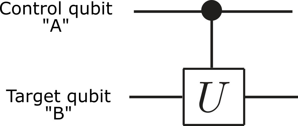
Figure 1.23: control unitary AB

Note that the roles of target and control qubit may be swapped [80]. A controlled unitary, $U_{B,A}^{c}$, with the B as the control qubit and A as the target qubit is denoted:

$$U_{B,A}^{c}=I_{A}\otimes\lvert 0\rangle\langle 0\rvert_{B}+U_{A}\otimes\lvert 1\rangle\langle 1\rvert_{B},$$ (1.31)

Where $I_{A}$ represents the identity gate operating on qubit A, and $U_{A}$ is the single-qubit gate that operates conditionally on qubit A. The quantum circuit of this controlled gate is shown in the following figure.

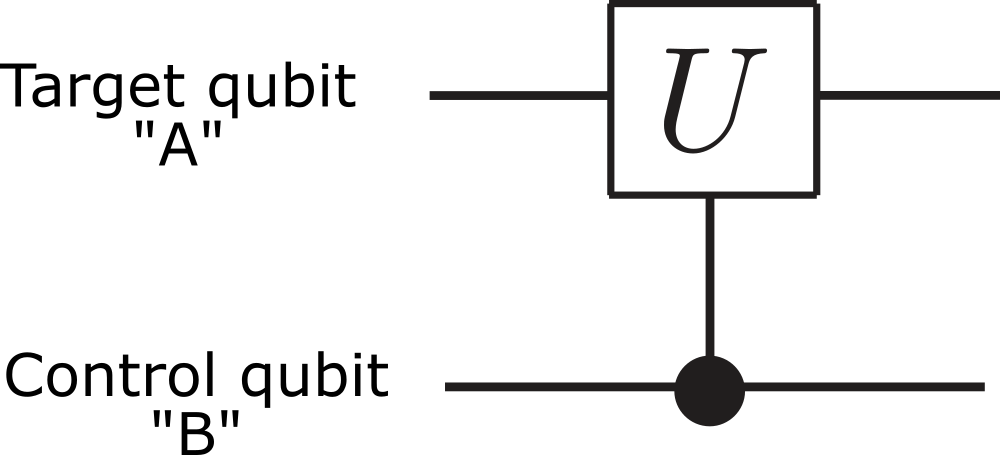
Figure 1.24: control unitary BA

Two common examples of conditional gates are the controlled-phase gate referred to as the CZ-gate and the controlled-NOT gate most commonly referred to as the CNOT-gate (it could also be called a CX-gate). Both gates take their name from the single-qubit operation U that is conditionally applied to the target qubit.

In the case of the controlled-phase gate, the conditional single-qubit operation is the Z-gate. The word “phase” refers to the phase factor $(\exp{i\pi}=-1)$ that results from an application of the Z-gate on state $\lvert 1\rangle$,

$$\begin{split}Z\lvert 0\rangle&=\lvert 0\rangle,\\ Z\lvert 1\rangle&=-\lvert 1\rangle.\end{split}$$ (1.32)

If qubit A is the control and B is the target, the controlled-phase gate can be written in Dirac notation as

$$Z_{A,B}^{c}=\lvert 0\rangle\langle 0\rvert_{A}\otimes I_{B}+\lvert 1\rangle\langle 1\rvert_{A}\otimes Z_{B},$$ (1.33)

and its quantum circuit is given by

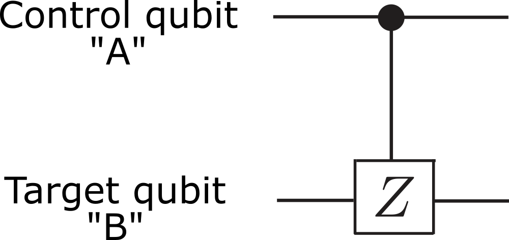
Figure 1.25: CZ gate

In the case of the CNOT gate, the single-qubit operation is the X-gate. The word “NOT” comes from the effect of the X-gate on the state $\lvert 0\rangle$ and $\lvert 1\rangle$,

$$\begin{split}X\lvert 0\rangle&=\lvert 1\rangle,\\ X\lvert 1\rangle&=\lvert 0\rangle.\end{split}$$ (1.34)

If qubit A is the control and B is the target, CNOT operator and its corresponding quantum circuit are:

$$CNOT_{A,B}=\lvert 0\rangle\langle 0\rvert_{A}\otimes I_{B}+\lvert 1\rangle\langle 1\rvert_{A}\otimes X_{B}.$$ (1.35)

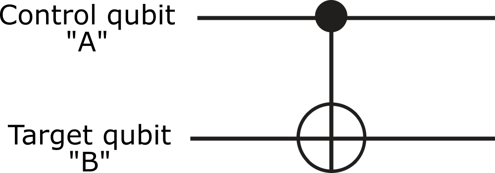
Figure 1.26: CNOT AB

Similarly, if the role of the control and target qubits are interchanged, the CNOT operator and its quantum circuit are:

$$CNOT_{B,A}=I_{A}\otimes\lvert 0\rangle\langle 0\rvert_{B}+X_{A}\otimes\lvert 1\rangle\langle 1\rvert_{B}.$$ (1.36)

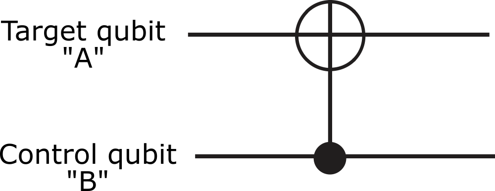
Figure 1.27: CNOT BA

A CNOT gate can be implemented using a Z-gate by applying a Hadamard gate, H, before and after a Z-gate, since X=HZH. The figures below represent this identity.

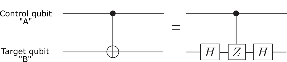
Figure 1.28: CNOT CZ Identity

The table below shows a summary of the two controlled-gates CZ and CNOT. Note that the sub-indexes A and B in $cZ_{A,B}$ are usually omitted. In their absence, it is generally assumed that the first qubit is the “control qubit,” and the second qubit is the “target qubit.” It is not only valid for the controlled-phase gate (CZ) but also the controlled-unitary gate (cU) and the controlled-NOT gate (CNOT).

Figure 1.29: Two Qubit

1.14   How Universal Algorithm Works

How is a universal quantum algorithm implemented on a quantum computer? In this section, we will have an intuitive introduction to how a universal quantum computer uses single-qubit and two-qubit gates to implement an algorithm.

Let us get an intuitive picture of how a quantum algorithm works. A universal quantum algorithm is built from a small set of single and coupled qubit gates. The input to a quantum computer is a massive superposition state, in general. Then, we apply the types of single-qubit gates that we have just discussed. The single-qubit gate operates on all the states simultaneously through quantum parallelism. It is followed by quantum interference, which modifies the coefficients in front of those states. We will also apply the types of coupled qubit gates that we have discussed, for example, the rotation of qubit y-depends on the state of qubit-x. Again, through quantum parallelism, these operations apply to the entire state space, followed by quantum interference, which will again modify the coefficients. Moreover, the goal of an algorithm designer is to ensure that, by the end of the algorithm, one of these coefficients has a value that is unity or very close to unity. It corresponds to the state that gives us the answer to the problem. It is a crucial point because we need to measure the output from the quantum computer to find the answer to the problem. The measurement process itself, in a quantum system, is probabilistic and leads to a classical result. So, although the output of the quantum computer is a massive superposition state, in general, the measurement process will project those qubits on to only one of the classical states that makes up the superposition. The probability that we get any given state corresponds to the magnitude squared of that coefficient. So, having a coefficient that is close to one or unity will give us a very high probability, the correct answer.

A quantum algorithm comprises a sequence of single-qubit and two-qubit gates. Quantum parallelism and quantum interference are used by the algorithm designer to take an input state typically a massive superposition state and, in a step-by-step manner, modify the weighting coefficients (probability amplitudes) until the quantum mechanical state evolves into an output state that encodes the answer to the problem. Since a projective quantum measurement will yield a single, classical state, it is imperative that the algorithm results in a final state with a probability amplitude near unity such that near-unity probability, the measurement will lead to the correct answer.

1.15   Universal Quantum Algorithm

What types of algorithms can be run on a universal quantum computer? What are the advantages, requirements, and challenges associated with universal quantum computation? In this section, we present a high-level introduction to universal quantum algorithms and quantum computation.

There are a couple of different kinds of quantum computers. The most general is a Universal Fault-Tolerant Quantum Computer. The gate model algorithm that we discussed earlier runs on this type of computer. Building a Universal, Fault-Tolerant Quantum Computer[81], we think, is one of the most significant scientific and technological endeavors today. Such a machine, when we build it, will have all the power that quantum has to offer. A Universal Fault-Tolerant Quantum Computer is a holy grail, in some sense, as it means we will be able to program, implement, and reliably run complex, large-scale quantum algorithms. We use a small set of single and two-qubit gates to implement universal quantum computation. In principle, this computer can run any type of algorithm-quantum or classical. However, there are only specific algorithms that are known to exhibit a quantum advantage. Something that We will refer to as quantum speed up. One example is Shor’s Factoring Algorithm. Shor’s algorithm is used to break public-key cryptography. For example, RSA encryption a scheme that is used for secure communications[82]. The security of RSA encryption is based on the premise that factoring a large integer number into two smaller prime numbers is a challenging computation for a classical computer to perform. The computational complexity scales poorly with the length of the encryption key. So, for example, if we are dissatisfied with our current security level, just double the length of our public key, and it will become exponentially harder for a classical computer to break that encryption scheme. In contrast, Shor’s algorithm can perform the same tasks, with only a marginal increase in difficulty, as the key’s length has increased. Other examples include Grover’s algorithm for searching an unsorted database [83], or sampling solutions to linear equations. For these types of algorithms, quantum speedup of some degree exists over known classical algorithms when run on a universal quantum computer[77]. The actual amount of speed up for these algorithms we will discuss later in the section. The advantage of a Gate Model Quantum computer is that it is universal. In principle, it can run any algorithm. Now, in practice, not all algorithms will exhibit a quantum speedup, but many will present. The challenge lies in making a computer that is both large enough and operates for long enough to complete an algorithm and obtain the answer. Even though the fundamental building blocks, the qubits themselves, are prone to errors. In a quantum computer, each operation has a probability of being noisy, That is of adding an error to the computation. We need a way to combat the build-up of all these errors so that the output we get out of the algorithm, or the computation is reliable. We will see later in the section; such errors can be overcome by something called Quantum Error Correction. However, it will require additional resources to implement it.

The power of a universal computer is that it can implement any algorithm that can be expressed in terms of a circuit comprised of logical gates. A universal, fault-tolerant quantum computer will enable people to program, implement, and reliably run arbitrarily complex quantum algorithms. In fact, a universal quantum computer can run any type of algorithm quantum or classical. Determining when it is advantageous to implement an algorithm on a quantum computer, as opposed to a classical computer, is one of the principal aims of quantum information science. The study of how efficiently a computer, whether a classical or a quantum computer, can solve a given problem results in the formal segregation of algorithms into what are called “computational complexity classes.” This efficiency is determined based on how the computational resources needed to solve a problem, grow, or “scale” with the size of the problem instance. For example, how the size of the memory or the number of computational steps scales with the problem size.

Two important computational complexity classes are P and NP[84, 85]. An example of a problem in P is the multiplication of two numbers of length n, which requires $n^{2}$ time steps to complete. For example, this means multiplying the binary numbers 01 and 10 requires 4-time steps since each number has n=2 digits, but multiplying 100 and 110 requires 9-time steps, since n=3 for these numbers. This time scaling, and any time scaling of $a\times n^{b}$ where both a and b are constants, is referred to as “polynomial scaling” and is considered efficient.

These problems should be compared with those in the complexity class NP, where the time required to solve a problem is exponential in the number of problem inputs and is therefore not considered to be efficiently solvable. An example of such scaling would be $2^{n}$. One common point of confusion is that time steps required to solve both P and NP problems can be comparable for small n. For example, when n=1,2,3, the given polynomial scaling requires time steps of $n^{2}=1,4,9,$ as compared to the exponential scaling, which requires $2^{n}=2,4,8$ time steps. However, as n increases, these two scalings rapidly diverge, and this is why they are categorized into different complexity classes. Considering n=10, these two scalings are already an order of magnitude apart, with $10^{2}=100$and $2^{10}=1024$. Go to n=100, and $100^{2}=10,000$, whereas $2^{100}>1\times 10^{30}$that is, 10 followed by 30 zeros! That is the power of exponential scaling. Finally, it is important to note that problems are classified into these categories based on the best-known algorithm for solving them and are therefore subject to change as discoveries are made.

One of the main reasons for the current interest in quantum computers is that specific problems can be solved in polynomial time on a quantum computer even though the best known classical algorithm for the same problem requires exponential time. A prominent example of this is Shor’s algorithm. Shor’s algorithm effectively factors large integer numbers into two constituent prime numbers, a computationally hard task for classical computers. The difficulty of Factorization is that it is used as the foundation for public-key cryptography[86], for example, RSA encryption. It is even using the best-known classical algorithm, the resources required to break RSA encryption using a classical computer increase exponentially with the length of the public key. Hence, the problem is considered to be in NP (although it has not yet been formally proven to be NP). Practically, this means that doubling the number of bits in an RSA encryption key makes it exponentially more difficult for a classical computer to break the scheme. In contrast, Shor’s algorithm can perform the same task efficiently on a quantum computer, with only a marginal increase in difficulty as the length of the key increases.

1.16   Quantum Simulation Emulation

Quantum computers can simulate a quantum system using both digital gates and analog evolution. They can also emulate a quantum system by tailoring the qubits and their connectivity. In this section, we will take a look at quantum simulations [87] and a specific example, nitrogen fixation. Another type of quantum computer is a quantum simulator [88], a processor that simulates a physical system’s behavior, a chemical reaction, or a biological process. Simulations can be implemented using single and two-qubit gates as on a universal quantum computer, and we will call these digital simulations. Alternatively, the qubits themselves, the way that they connect, and the strengths of those connections can be designed to emulate a system’s behavior. We will call this an analog simulator. There are also examples of hybrid simulators [89]that use aspects of both digital and analog approaches [90]. Nature is quantum mechanical. So, with quantum computers, we get this ability to take a step closer to being able to computationally model aspects of physical systems. So, we think this is a pretty fantastic potential first application of quantum computers. As the first business application, with the knowledge of today, we would say the simulation of molecules in materials [51] is the most likely, which, in turn, can have a broad impact on science, technology, and society. One example is the simulation of chemical reaction mechanisms. It is estimated that somewhere between 1% and 2% of worldwide energy production is used to produce ammonia for agricultural fertilizer. The critical step is a process called nitrogen fixation. In industry, nitrogen fixation is performed using the Haber Bosch process, which requires both high pressure and high temperature. In contrast, there exist bacteria that use an enzyme called molybdenum nitrogenase, which, even at room temperature, can catalyze atmospheric nitrogen into ammonia. How do the bacteria do it? we do not know precisely. We do know the critical component is an iron-molybdenum cofactor, a chemical compound that acts as a helper molecule for the enzyme. However, it is not known how the reaction works in detail. Simulations with classical computers, exist but only provide approximate answers. If we could study that process and understand it, we could potentially engineer a catalyst that makes this reaction efficient. Now to study this with classical computers, this is the lifetime of the universe time scale to get a solution. On the other hand, quantum simulation of the chemical reaction steps would provide the reaction energies involved in the nitrogen fixation. This type of quantum chemistry simulation has many applications[91, 92, 93]. For example, developing new pharmaceutical drugs or tailoring a material to have unique properties. For these types of simulations, it has been shown that a quantum speedup can exist over known classical algorithms.

Quantum computers can be applied to many types of simulation problems. The challenge is that many of these problems require large numbers of well-behaved qubits, and such large-scale quantum computers are still likely a decade or more away. Before we get to the point where we can simulate systems entirely on quantum computers, there may be room for hybrid classical-quantum systems to hold a quantum advantage over purely classical algorithms[77]. One example is called a variational quantum eigensolver, another hybrid quantum-classical algorithm is Variational Quantum Fidelity Estimation[94],variational quantum factoring (VQF) algorithm[95].

A variational quantum eigensolver [96, 97, 98, 99, 100, 101, 102, 103] determines the lowest-energy state of a quantum system, a difficult task of importance to quantum chemistry. The protocol goes as follows:

1. The quantum processor is set so that it simulates the dynamics of the quantum system of interest

2. The classical computer proposes a trial ground state, which is then loaded into the quantum processor

3. The quantum processor calculates the energy of that state and passes it back to the classical computer

4. The classical computer takes that value for the energy and uses it to generate a new ground trial state, one which should give a lower energy

5. This process repeats until the VQE cannot find a new trial state that gives yet lower energy. This state is then likely the lowest-energy state of the system.

A vital aspect of this process is that the classical computer is not merely being used to initialize a quantum computation; the classical and quantum computers are passing information back and forth throughout the simulation. Therefore, the quantum computer is acting as a co-processor. It need not be coherent over the entire duration of the simulation, but only over the period of time, it takes to simulate the energy of a single trial state. This approach may allow useful computations to be done in the nearer term using less reliable qubits.

The VQE method has been shown to successfully determine the molecular spectra [104]of a hydrogen molecule $H_{2}$. To simulate the hydrogen molecule comprising two electrons, a quantum processor with 2 superconducting qubits is sufficient [105]. It has also been used to simulate other small molecules, such as $BeH_{2}$. All of these simulations to date are prototype problems that demonstrate the mechanics of the quantum simulation, but the problems themselves are easily solved on a classical computer. As the number of qubits increases, VQE can be applied to larger, more challenging simulations.

1.17   Quantum Annealing

A quantum annealer is a different type of computer that addresses classical optimization problems by mapping them onto a set of interconnected qubits and then searching for a solution (or solutions) that minimizes the total energy. In this section, we will get a high-level introduction to quantum annealing computers and how they work.

The third type of quantum computer is called a quantum annealer, and it is used solely to solve classical optimization problems. Optimization problems are those that we face every day. What is the best way for us to be able to drive home when there is traffic? What is the best way to route aircraft around an airport? All of those are optimization problems. If we are planning a very complicated mission, space mission with many moving parts that involve materiel, people, gasoline, if we can optimize and improve the efficiency of something like that, quantum computing could have a considerable impact. Quantum annealers do not use digital gates. Instead, an optimization problem is encoded directly into the qubits and their connectivity to one another, and by the strength of those connections. Finding the qubit states that then minimize their total energy is equivalent to optimizing and finding an encoding problem. However, how do we anneal these qubits into states that minimize their energy? So, the name quantum annealing is related to making a sword, where we take a piece of metal, and then we heat it, and in the old days, a swordsmith would beat the sword into some shape, and they would cool it, quench it in water heat it up again, and then beat it into shape and do that multiple times. Furthermore, that was called an annealing process. So, heat it, cool it down, heat it, cool it down. Quantum computing uses a similar technique. To perform annealing, we start by setting the qubit states and their couplings to one another in a configuration where we know the ground state. Let us call this the starting configuration or its starting Hamiltonian. We then slowly change the qubits and their couplings from those in the starting Hamiltonian to those in the encoded problem Hamiltonian [106]. Now, if we make these changes slowly enough, it is likely that We will remain in or very near the ground state of the system so that by the end of this evolution, the qubits are in their ground state, and that represents the solution to the optimization problem. If we have a problem that we can craft as a landscape like the Alps, for example, what the computer does is, without adding or subtracting, it would find the lowest valley or valleys in that landscape. It is probabilistic, and again, does not add or subtract, but rather, it is not a three-dimensional version of the Alps. However, it is an n-dimensional energy landscape, and it is finding a low energy solution to that problem. The challenge is that for problems of unusual size and complexity, it is almost certain that no matter how slowly we change these parameters, the annealer will, at some point, leave its ground state. It is due to the more significant number of energy states and their proximity to one another and as a result, quantum annealers must find additional mechanisms to return the computer to the ground state, for example, through quantum tunneling or by introducing excess relaxation, a loss of energy that returns the computer to its ground state. If we hit a barrier like a mountain range, as we described earlier, what the machine does is rather than we have to put more energy to climb the mountainside and go down the other side, we use the quantum mechanical property of tunneling. We tunnel through the barrier to get to what should be a lower energy solution in the next valley if we will. On the other hand, add too much relaxation and the computer may not even be quantum mechanical anymore. As a result, it is currently unknown if a quantum annealer can exhibit quantum enhancement for a general class of optimization problems. It may just represent another type of classical computer. Although, as a classical computer, it would not scale well with the size of the problem. However, it may still be interesting if it were substantially faster than any of today’s transistor-based classical computers. Volkswagen, in March of 2017, announced the optimization of about 500 taxis going from downtown Beijing to the airport, always congestion used the machine to see if we could come up with optimized routes for each of those taxis to get everyone moving more quickly. Worked, but it is a prototype application. Could not yet handle all the vehicles in Beijing, for example. There are technical challenges facing quantum computing. For the quantum annealing computers, how do we scale them up to be able to start attacking more real-world problems instead of subsets of real-world problems? There has a keen interest in quantum annealers because classical optimization problems are everywhere, from supply transport optimization to sensor and satellite tasking, pattern recognition[107], needle in a haystack problem. Many problems can be reduced to optimization, and so there is an extensive application pull to understand quantum annealers better.

The third type of quantum computer is a quantum annealer, an “application-specific” computer that is used solely to solve classical optimization problems. Quantum annealers do not use digital gates. Instead, an optimization problem is encoded directly into the qubits and their interactions (qubit interaction is referred to as coupling). Minimizing the total energy of the system is equivalent to optimizing and finding an encoding problem.

To quickly explain some physics jargon: Every quantum system has some amount of energy that is determined by the state of each object (e.g., each qubit) in the system. The state of each individual object, in turn, determines the global state of the entire system, and each global state corresponds to the system having particular total energy. The Hamiltonian is a function that matches each state to an energy value. So, for our purposes, the Hamiltonian is a function that tells us “if our qubits are in the state $|\psi\rangle$, our system has energy $E_{\psi}$. The state that gives the lowest energy for a system is called the ground state.

The idea behind quantum annealers is that if we have a quantum system governed by one Hamiltonian, we can transfer it to another Hamiltonian by changing the system’s parameters.

Quantum annealing starts with a qubit state configuration for which the ground state is well known. It is the starting configuration or starting Hamiltonian. By gradually turning off the starting Hamiltonian, while turning on the problem Hamiltonian, one can transition to the configuration that encodes the problem. If this transition is performed slowly enough and the system has no noise, then the computer will remain; it is ground state throughout the evolution. Measuring the state of the computer in the final configuration yields the answer to the problem. As described here, this is an “adiabatic quantum computer.”[108, 109]

The challenge is that for problems of unusual size and complexity, it is almost certain that no matter how slowly the coupling parameters are changed, the annealer will leave its ground state. There are two primary reasons for this: first, the “minimum gap” between the ground state energy and nearby excited-state energy levels gets very small as the size of the problem increases; and second, there is always noise in the system due to non-zero temperature. Although operation in a cryogenic environment reduces noise, it does not eliminate it [110]. as the minimum gap gets smaller eventually, even cryogenic temperatures begin to look relatively “warm.”

Consequently, quantum annealers must find additional mechanisms such as quantum tunneling or excess relaxation to keep the computer in the ground state. On the other hand, too much relaxation will make the computer manifestly classical. As a result, it is presently unknown if a quantum annealer can exhibit quantum enhancement for a general class of optimization problems or whether it is merely another type of classical computer. Nevertheless, there is intense research into quantum annealers today, because the application pull is strong. Many real-world can be cast as optimization problems (e.g., financial portfolio optimization [111], product distribution, routing of autonomous vehicles[112]), and so there is a strong motivation to understand quantum annealers better. Quantum annealing is a method for finding solutions to classical optimization problems. The quantum annealer encodes the problem on to a set of qubits and biases those qubits into a starting state with a known ground state (that is not the solution to the problem). The system is then slowly evolved towards a set of bias points that do represent the problem being solved, and the ground state of the system is the answer to the problem. However, a quantum annealer is likely to leave its ground state during this evolution. The concept is that, though a combination of quantum tunneling and relaxation processes, the system should find its way back to the ground state (or a lower-energy state) to find the encoded (approximate) solution to the optimization problem [113].

1.18   The DiVincenzo Criteria for Quantum Computers

There are a variety of physical systems that have been proposed as the qubits for quantum computers. What properties must a given technology possess in order to build a quantum computer? In this section, we will discuss the DiVincenzo Criteria[114, 115], the minimum set of requirements a qubit technology must have to be considered a viable candidate for quantum computing, and for communicating quantum information.

There are numerous examples of quantum mechanical two-level systems in nature that could potentially serve as qubits. For example, the electronic states of an ion, or the electron spin of a phosphorus atom implanted in silicon [116] or a nuclear spin of a defect in diamond. We can even manufacture electrical circuits that behave as quantum mechanical two-level systems or artificial atoms. However, what makes a useful qubit? Furthermore, how do we assess these qubit modalities and compare them to one another? Furthermore, how can we determine if a modality is well-suited for quantum computing? We can begin to answer these questions by first drawing on the intuition from classical computing. What makes an excellent classical logic element? Furthermore, why did we end up with transistors? If we want to build a computer at a scale large enough to perform new problems, we should start with a technology that scales well, one where we know how to define and characterize the logic elements and where we can manufacture them in large numbers. These devices must also accurately represent and process classical information. We need to set their states to provide input to the computer, and we need to be able to measure the result to get an answer. Finally, these devices must be robust against failure to complete the computation and reliably obtain the answer. Transistors satisfy all these requirements very well, so it is no wonder that today’s computers are built from transistors and not, vacuum tubes, or mechanical switches. So, what makes a useful qubit? Around the year 2000, David DiVincenzo, then a researcher at IBM, articulated five necessary conditions that any qubit technology must at least possess for a suitable physical implementation for large scale quantum computation [115]. First, it should be a scalable physical system with well-defined and characterized qubits. Second, we must be able to set the input state and, third, measure the resulting output state. Fourth, we must be able to perform a universal set of gate operations. For example, the single and two-qubit gates that we discussed previously that are needed to run an algorithm. Fifth, the qubits must robustly represent quantum information. In many ways, these requirements are like those for classical computers. It is only in how the requirements are met that we can identify differences—for example, performing a universal set of one-qubit and two-qubit gates rather than universal Boolean logic. Alternatively, to robustly represent quantum information, qubits must have long coherence times[117], a concept that loosely translates to the meantime to failure for a transistor. In addition to these five requirements for the qubit technology, David DiVincenzo added two conditions related to the communication of quantum information between qubits. So, continuing from number five, number six is that the technology must support the interconversion of quantum information between a stationary qubit and a flying qubit. Moreover, seven, there must be a way to transfer flying qubits faithfully between two locations. These two requirements describe a quantum version of an interconnect that is, the means to take the quantum information encoded in one qubit, convert it to an object that can move, like a photon, provide the means to guide a photon without loss to another qubit at a distant location, and then hand back that quantum information. Again, analogous to requirements for routing signals within a classical computer but following the rules of quantum mechanics. These criteria, today referred to as the DiVincenzo Criteria, articulate the basic requirements that any qubit technology must possess if it is a viable physical implementation for quantum computation.

Several quantum mechanical two-level systems potentially could serve as qubits. For example, the electronic states of an ion, the electron spin of a phosphorus atom implanted in silicon, a nuclear spin of a crystal defect in diamond, and even manufactured “artificial atoms,” electrical circuits can be described as quantum mechanical two-level systems. What are the basic requirements any one of these modalities must at least possess to be a candidate for a quantum computing technology?

In 2000, David DiVincenzo, then a researcher at IBM, articulated five fundamental requirements for any qubit technology to be a suitable physical implementation for large scale quantum computation (see the paper here [115]).

In addition to these five criteria for qubit technology, David DiVincenzo added two conditions related to the communication of quantum information between qubits.

Figure 1.30: DiVincenzo Criteria

These criteria, known as the DiVincenzo Criteria, are, in many ways, adapted from the conditions for classical operational computers and summarize the fundamental requirements qubit technologies need to fulfill at a minimum to be a candidate quantum computing technology.

1.19   Qubit Coherence and Gate Time

In this section, we will discuss two types of errors that can occur in qubits energy relaxation and decoherence and their corresponding characteristic lifetimes $T_{1}$ and $T_{2}$. We will also consider the clock speed at which qubit operations can be performed[118].

The average number of operations that can be performed within a qubit lifetime is a proxy for a more rigorous metric called gate fidelity. Implementing more operations before an error occurs is good. As we will see in this section, longer coherence times do not necessarily translate to more operations per gate time, as the gate operations themselves are generally slower in long-lived qubit modalities. However, just as with classical computers, there is a distinct advantage to faster clock speed, as that means we obtain results faster.

The DiVincenzo criteria articulated the requirements that a qubit technology must have to be a viable candidate for the physical implementation of a quantum computer. In this section, we will build on two of those criteria, related to qubit robustness and quantum gates, to define metrics that will allow us to compare qubit modalities with one another. To do this, let us first look, in more detail, at the qubit coherence time, the analog of the meantime to failure for a transistor. Quantum computers, like classical computers, must be built from robust elements. The coherence time is one metric that quantifies the robustness of a quantum bit. Essentially, it is the amount of time, on average, that a qubit state is maintained before the quantum state is lost. As an illustration, let us consider a qubit that we set into a quantum state psi, and consider what happens to that qubit over time. At first, the state is well-defined, we just put it in that state, we are confident that we did a good job, and so we know what the state is. Over time, however, the qubit begins to interact with its environment. When it does so, the qubit experiences noise that alters the qubit state in ways that we did not anticipate. Intuitively, we can imagine that the state begins to blur. as time goes on, and the qubit is subject to more of this environmental noise. Eventually, we can no longer recognize the state, and the quantum information is fully lost. The qubit is still there, but it is no longer in the state that we would have expected it to be in after this amount of time. The noise has altered the behavior of the qubit, and it is now in some other state. Let us now look at how we quantify qubit lifetimes, by looking at errors on the Bloch Sphere. There are two fundamental ways in which a qubit loses quantum information. The first is energy relaxation. Imagine that we put the qubit in its excited state, state 1. Unfortunately, it probably will not stay there, due to noise at the qubit frequency, the qubit will, at some point, lose its energy to the environment and return to the ground state. This loss of energy is called energy relaxation, and on average, it occurs after a time called $T_{1}$. The second way a qubit can lose quantum information is through a loss of phase coherence. Imagine that we intentionally set the qubit at one point on the equator of the Bloch Sphere. It likely will not stay in that direction forever, due to interactions with the environment. there are two ways that phase coherence can be lost. First, the qubit state may move around on the equator, due to the environmental noise. If we repeat the experiment often, the noise will sometimes drive the Bloch vector east along the equator, sometimes to the west, and over time, the Bloch vector fans out more and more. It does this until, eventually, we can no longer tell which direction, or equivalently, which phase, the Bloch vector has. the average time it takes for this to happen is called the pure dephasing time, $T_{\phi}$. Now there is another way things can go wrong on the equator. Remember that, on the equator, the qubit is in a superposition state of 0 and 1, with 1 being the excited state. If that component of the superposition state loses its energy to the environment, then the 1 state flips to 0, and the superposition state is lost. Essentially, the qubit is relaxed from the equator to the north pole. Energy relaxation is also a phase breaking process since once the Bloch vector points to the north pole, we can no longer tell which way it had been pointing on the equator, that phase information is lost to the environment. Thus, the average amount of time that a qubit remains coherent is related to both the dephasing time, $T_{\phi}$, and the energy relaxation time, $T_{1}$, which together give a time $T_{2}$, over which phase coherence is lost. Thus, a qubit loses its quantum information by two mechanisms, energy relaxation and loss of phase coherence, characterized by the times $T_{1}$ and $T_{2}$. Now another important metric for quantum computers, just as with classical computers, is the clock speed, the time required to perform a quantum operation. It is called the gate time, and although it generally differs for single and two-qubit gates, we can use a typical time, or conservatively, use the slowest gate time, to define the clock speed with which we can operate the quantum computer. as with all computers, faster is better. Even if we have an exponential speedup from a quantum algorithm, it still takes some time to perform that algorithm. All else being equal, a faster clock speed will translate to obtaining the answer more quickly. A key figure of merit, then, is the number of gates one can perform within the qubit lifetime. The more gates one can implement before an error occurs, the larger an algorithm one can run. This metric also illustrates an interesting trade-off with qubits. In general, qubits with long lifetimes have less interaction with their environment. That is good because they have less sensitivity to noise. However, the trade-off is that they respond more slowly, even when we intentionally try to control them. It is because They are not just weakly interacting with their environment. They are also weakly interacting with the control fields. Similarly, qubits that more strongly interact with their environment may have shorter coherence times, but they generally respond faster. The number of gates one can perform, on average, before an error occurs, may not differ much between these two cases. However, one of these qubit modalities may have a much faster clock speed than the other one, and that is a good thing. This figure of merit, the average number of gates one can perform before an error occurs, is a proxy for a more general and rigorous concept, called gate fidelity, which We will discuss next.we would like to understand if a quantum processor will have the same limitation of classical processors regarding the gigahertz and clock speed hardware. It is possible to have a or is it possible to have a quantum CPU with much more than with many more gigahertz than is typical nowadays at 3 gigahertz? that the clock speed matters whether we are discussing about classical or quantum computers from the point of view of it will take a certain amount of time to solve a problem. if we want to solve that problem faster, then we need to run the computer faster. But we think making a comparison between classical clock speeds and quantum clock speeds is not really the right comparison because, as we know, a classical computer can really get bogged down on some of these hard problems that a quantum computer can solve very efficiently. so, a problem like factorization, which might take the age of the universe on a classical computer so, just completely impractical on 100-megahertz quantum computer might be able to do this factorization could be done in about an hour or a couple of hours. that is for, a 2,000 or 4,000-bit number. So, that has nothing to do with clock speed. That has to do with quantum computing being a fundamentally different computing paradigm than classical computing. But then what we discuss and we think this is an important point, is that if we have a quantum computer and it can do that calculation in a day at, 100 megahertz, fantastic. It did not take the age of the universe. It took a day much more efficient, exponentially more efficient. But if we run on another quantum computer that is 1,000 times slower, then that will take 1,000 days. so, there, the speed actually matters. So, within quantum computing paradigm [119, 120], comparing different computers, it makes sense to discuss about gate speed. But we also want to emphasize that It is not just gate speed. So, it is gate speed, assuming that all else is equal, meaning that we have two computers and they have the same connectivity, the same overhead for error correction. If they are identical in and along all of those axes, then clearly, running one 1,000 times faster is going to give we an answer at 1,000 times sooner. But gate speed is not the only thing that determines how fast we achieve a solution. the degree to which qubits can be connected to one another for example, do we only have in array of qubits, we only able to connect to a nearest neighbour or do we have an all-to-all connectivity? Can every qubit discuss through a two-qubit gate directly to any other qubit in the system? That is a huge difference. That makes a tremendous difference in the execution speed. So, it is not just clock speed that matters. But clock speed does matter, as explained.

There are two processes by which a qubit loses quantum information. The first is called energy relaxation, and it is characterized by time $T_{1}$. It is characteristic time it takes for a qubit in its excited state to relax back to its ground state by emitting energy to the environment. It can be visualized on the Bloch sphere as a qubit prepared in the excited state (south pole) switching to the ground state (north pole) through energy loss. $T_{1}$ also characterizes the time over which a qubit will absorb energy from the environment. However, most leading qubit technologies today operate in a regime where such energy absorption processes are negligible compared with energy decay.

The second way a qubit loses information is through decoherence. There are two ways for a qubit to lose coherence. The first is that due to environmental noise, a Bloch vector on the equator might move along the equator away from it is the original position in a manner we cannot predict, and over time, we lose track of which way the vector is pointing. It is called dephasing, and it occurs over a characteristic time $T_{\phi}$. The second is that the excited-state portion of the qubit superposition state could lose its energy to the environment, and the qubit “falls off” the equator and back to the ground state (north pole). It is also a phase-breaking process since once the vector is at the north pole, we can no longer tell which way it had been pointing on the equator, and it occurs over the same characteristic relaxation time, $T_{1}$. Together, these two dephasing mechanisms lead to the decoherence time $T_{2}$, which is a function of the dephasing time and the energy relaxation time: $1/T_{2}=1/T_{\phi}+1/2T_{1}$.

Mitigating the resulting errors can be quite challenging on quantum computers, much more so than correcting classical errors on conventional computers. For example, one can periodically error-correct a bit by simply measuring and resetting its state on a classical computer. For example, a classical bit might be stored as a voltage, where a voltage of 5V denotes a 1, and 0V denotes a 0. Even though we cannot assume that a bit set to 1 will stay at 5V forever, we can periodically measure it is voltage and reset it to 5V if it starts to decrease.

In contrast, because of the way measurements affect quantum systems, this option is not directly available to us in quantum computers. It is not possible to measure a state and then reset it precisely, because making that measurement disrupts the quantum state of the system in a manner that is not entirely reversible. It is why we work very hard to shield qubits from environmental noise in the first place. Still, there are quantum versions of error mitigation and error correction that can fix residual errors, provided the underlying qubits are “good enough”.

1.20   Gate Fidelity

How does one confirm that a gate operation is working as intended? In this section, we will discuss the gate fidelity of a quantum operation. Gate fidelity quantifies the quality of gate operation, and it is used to compare qubit modalities of varying types.

In the last section, we focused on two of the DiVincenzo criteria, qubit coherence, and quantum gates. We developed an intuitive figure of merit, the average number of gate operations that can be performed before an error occurs. Such metrics are important because they allow us to compare different qubit modalities, even when those modalities have remarkably different properties. However, the definition we introduced only accounted for errors due to qubit decoherence. That is fine for qubits dominated by decoherence, but other sources of errors limit some qubit modalities. For example, control errors, imperfections in the pulses that are used to drive a gate operation. For these qubits, even if their coherence times were practically infinite, their gates would still be subject to control errors. So, we need a more rigorous way to characterize the robustness of gate operation, one that is sensitive to a broad set of error sources. that leads us to this section’s subject, a more general concept called gate fidelity. Gate fidelity is a rigorous means to define how well a gate operation works. Essentially, it is a measure of how closely the actual gate operation matches, on average, a theoretically ideal version of that operation. For example, if we apply an X-gate to a qubit prepared in state 0, how close do we get to state 1? Now intuitively, errors could occur along any direction of the Bloch Sphere, and so we need to check for errors along with all directions after the operation is complete. Until this point in the section, we have only measured the qubit along the Z-direction. In principle, we can measure the qubit along any axis that passes through the center of the Bloch Sphere, including the x-axis or the y-axis. Besides, gate errors may be manifest differently, depending on the starting point of the qubit, so we need to check how the gate performs against different initial states, and not just the north pole, for example. Now at this point, we may be asking ourselves, how is this even feasible? The qubit state can be anywhere on the surface of the Bloch Sphere, representing an infinite number of possible initial and final states. How can we possibly check them all? Well, we do not have to. That is because we can define a basis set that spans the entire qubit state space. To draw an analogy, think of global positioning. the position anywhere on the globe can be represented by projecting it onto a convenient basis, in this case, a coordinate system that spans the globe. We often use latitude and longitude, but we could equally use Cartesian coordinates, x-, y-, and z. Similarly, we can define a basis that spans the entire qubit state space, and then use it to specify any qubit state at the input. We can also use it to characterize any state at the output, by projecting back onto this basis. It works because quantum mechanics is described by linear algebra. It is enough to understand projections to and from the basis set to know what will happen globally. We will see in the section later, and such projective measurement plays a crucial role in the digitization of errors and the ability to correct them. Although the coefficients of a superposition state will dictate the probability of obtaining a 0 or 1 when the measurement is done, for any given measurement, we will get a 0 or a 1. In this way, quantum states and their errors, which appear to be analog, can be digitized through projective measurement. Now we discuss previously that n-qubits could represent $2^{N}$ states. Here, the basis can be represented in a matrix form, and the number of matrix elements that span the state space is the square of the number of states. So, $2^{N}$, quantity squared. For a single qubit, n equals 1, and we need four elements. For two qubits n equals 2, and the number quickly increases to 16. So, determining the gate fidelity is essentially a standard black box type problem. We have a gate operation, and theoretically, we know how it should perform. However, due to errors, its actual operation is not precisely known. That is the black box. Thus, we need to characterize, on average, how well the gate operation performs. To do this, we probe the gate operation using the input basis states, perform the actual gate operation, and then, for each input, project the resulting output state onto the entire basis set. We then compare the results to what we would expect from a theoretically ideal operation to determine the gate fidelity. The described approach is called process tomography [121], and it represents a complete description of the errors during a gate operation. It also requires many steps to implement, as the product of input and output elements is $2^{4N}$. Now, although there are $2^{2N}$-th constraints, due to the properties of these matrices, this only reduces the total number of measurements by a small amount. Thus, implementing process tomography scales very poorly with the number of qubits, and becomes impractical as n gets large. This is an issue, because although the gates only act on one or two qubits, the errors may leak to nearby qubits, qubit 3, qubit 4, or qubit 5. Thus, to account for this, the basis we choose must encompass all n qubits. Besides, process tomography is sensitive to all errors, including initialization errors, when preparing the input state, and measurement errors at the output, which, although certainly real errors, are unrelated to the quality of the gate operation itself. As a result, an alternative approach, called randomized benchmarking [122, 123, 124, 125], has also been developed. Randomized benchmarking essentially interleaves the gate operation being characterized by a random assortment of other gate operations[126]. Although half of the gates are chosen at random, we know what they are, and so we can predict the expected output state, assuming all the gates were ideal. It is then compared to the same experiment, but with only the random assortment of gates, to see how much the error rate has changed when adding the interleaved gate. This change in error rate is then attributed to the interleave gate itself. This approach is repeated for increasing numbers of pulses to obtain a refined estimate for the average error per gate and, thereby, the gate fidelity. Randomized benchmarking is much more efficient than process tomography, and it is also insensitive to initialize and measurement errors. However, it only provides a net error rate without revealing specific error channels. However, it is measured, a gate fidelity of 100% means that the actual operation perfectly matches the ideal operation. For example, no matter where the qubit starts on the Bloch Sphere, the actual x-gate would perfectly rotate the input state to the correct output state. Now, as we might expect, it is generally not possible to achieve a perfect gate fidelity. There will always be some level of error, whether due to qubit decoherence during the operation, imperfections in the control pulse itself. The goal is to see how many nines, two nines, 99%, three nines, 99.9%, that one can achieve. The higher the fidelity, the closer it comes to an ideal gate. We will see later in the section, achieving high fidelity is critical, because it translates directly to two important aspects of quantum error correction. First, the fidelity must at least reach a minimum value, called the threshold, for the error correction to give us a net improvement in the error rate. second, once above this threshold, the higher the fidelity, the less the resource overhead required to implement the error correction.

Gate fidelity is a metric that characterizes how well a gate operation works. Intuitively, we are asking the question: how close does the actual implemented gate operation come to an ideal, theoretically calculated one?

To answer this question, we need to consider all potential errors that may impact the gate operation and the resulting qubit evolution. These errors can, in principle, arise from any direction on the Bloch sphere, so we need to check the fidelity for different starting states of the qubit. Similarly, we need to assess the qubit’s final state in all directions along which errors may occur.

To do this, we define a basis set for the qubit that spans all of the possible qubit states and qubit operations. Global positioning is an analogous concept, where we can identify our position on the planet earth using a basis of longitude and latitude, or, equivalently, we could use the Cartesian coordinates x-, y-, and z. Similarly, since quantum mechanics is governed by states and operators that follow linear algebra rules, we can define a basis for the qubit states and operations.

Qubit state tomography is the projection of a qubit state onto this basis[69], and it fully characterizes a qubit state (its position on the Bloch sphere, for example). Similarly, process tomography fully characterizes a gate operation. Since a gate may be applied to any qubit input state, we must first prepare the qubit in each of the basis states that span the possible input state-space. Then, for each of these inputs, the gate operation is applied, and the resulting output state must then be projected and measured against the entire set of basis states at the output. This process is then repeated for each input state. Ultimately, the net results are then compared to a theoretical gate operation, and the “distance” between the two results quantifies the gate errors.

The number of elements in the input matrix that represents the basis states for N qubits is $2^{2N}$, and there is the same number of elements in the output matrix. Since the gate operation must be applied to each input state, and the result in turn projected on to each of the output states, the total number of input-output combinations is $2^{2N}\times 2^{2N}=2^{4N}$. For a single qubit, this is 16; for two qubits, the number quickly increases to 256. while there are a few constraints that will reduce these totals by $2^{2N}$, the net number of combinations that must be measured is only reduced to 12 and 240, respectively. It is another example of the power of exponential growth, but, in this case, the rapid expansion in the number of states works against us. We must make all of these measurements to characterize the gate entirely. Besides, process tomography is sensitive to state preparation and measurement errors commonly referred to as SPAM errors. While SPAM errors are real errors, they are independent of the gate operation and should not be included in the gate fidelity.

An alternative approach is called randomized benchmarking. Randomized benchmarking characterizes a gate operation’s aggregate performance by interleaving it with a random (but known) assortment of other gates[127, 128]. The random gates are first characterized by themselves to assess a baseline level of error, including SPAM errors. Then, the same measurement is performed with the desired gate operation interleaved into the sequence. The outputs are then compared, and the net additional error is attributed to the addition of the desired gate operations. This process is repeated while increasing the number of gates to refine an estimate for the net error per gate. In this way, randomized benchmarking provides an aggregate fidelity that is somewhat more efficient to implement and is ideally independent of SPAM errors. The trade-off means that it averages all error channels without quantifying each individually (as is possible with process tomography).

Gate fidelity is a crucial metric that allows us to compare remarkably different qubit technologies on an equal footing. Gate fidelity is a benchmark that determines the feasibility, efficacy, and resource overhead required for implementing quantum error correction.

1.21   Qubit Modalities: Electron and Nuclear Spins

There are several physical manifestations of qubits. In the next three sections, we will discuss several qubit modalities. In this first section, we will be introduced to physical qubit modalities based on electron and nuclear spins. In the second section, neutral atoms and trapped ions. In the third section, superconducting qubits and other modalities.

Until this point in the section, we have generally discussed qubits as quantum mechanical two-level systems. However, how do we physically realize a qubit in practice? Moreover, what are the leading physical realizations today? In this section, we will have a general introduction to several candidate qubit technologies. Later, we will present an in-depth look at two of the leading qubit modalities. Let us start with electron spin. As in the introduction to quantum parallelism and quantum interference, the electron spin has two states, spin up and spin down. The question is how to isolate a single electron. In this first example, the electron spin is trapped in a quantum dot, a small region of semiconductor material where a single electron can be trapped. We start with a two-dimensional sheet of electrons called a two-dimensional electron gas, which can be realized at the interface of a slab of silicon and a slab of silicon germanium. Metallic gates are then defined on the surface of the device to define the quantum dot region electrostatically, and by applying the appropriate gate voltages, a single electron spin can be trapped there. Combinations of microwaves and baseband pulses are then used to implement quantum gates. Now we will find several key properties of quantum dot qubits shown here. We will not read through them all, as we can find them in the table associated with this section. In the next section, we will make comparisons between qubit modalities based on these numbers. Now, in addition to the single dot shown here, there are also more complex designs, including double dots, triple dots, and even dots based on CMOS devices. Each of which adds complexity to gain certain advantages. In general, the main attraction of quantum dots is that they leverage advanced silicon fabrication technology[129], two, they are relatively small in area and so in principle can be integrated into large numbers. Three, much like CMOS, they are controlled using gate voltages. The main challenge is that multiple gates are required to define a single qubit. Thus, 3D integration techniques will certainly be required to realize large scale circuits. Another example of an electron spin qubit is in phosphorus-doped silicon [130]. Here phosphorus atoms are implanted in the silicon substrate, and the spin-off of its outermost electron serves as the qubit. As with quantum dots, electrostatic gates control the qubits using a combination of the baseband, RF, and microwave pulses. The main advantages of phosphorus-doped silicon are that it also leverages silicon fabrication technologies. The electron spin qubit has very long coherence times[130]. The primary challenge is that the dopants must be close to one another, around 10 nanometers, to have a sufficiently large two-qubit coupling to implement a two-qubit gate. It makes it extremely challenging to place the gates and route the wires required to control the qubits. It also means that crosstalk between control lines and qubits will be significant. Again, 3D integration will be required here. A second challenge is that the phosphorus dopants must be implanted in the silicon with very high precision. This remains an outstanding challenge. Phosphorus dopants also have a nuclear spin that can be used as a qubit controlled using radiofrequency or RF pulses. The main advantage of nuclear spin qubits is their extremely long coherence times, which arise because the spins are largely decoupled from their environment. The trade, though, is that the gate times are rather slow. A second system that affords both an electron spin and a nuclear spin is the nitrogen-vacancy center in diamond. Diamond is formed from a tetrahedral lattice of carbon atoms. Occasionally, however, a defect interrupts this lattice, and one example is called a nitrogen-vacancy [131], in which a nitrogen atom is injected into the lattice and causes the carbon vacancy to form. The result is an extra pair of electrons that form a spin 1 system, which is the lowest 2 spin levels that can be used as the qubit. Alternatively, the nuclear spin of the nitrogen atom, or the surrounding carbon atoms, may also be used as the qubit. The electron spin is addressed by a combination of microwave pulses to implement the quantum control and lasers to initialize and measure the qubit. The nuclear spin has a magnetic field dependent splitting that is controlled at radio frequencies. The advantage of NV centers is that they are rather well-suited to the interconversion and communication of quantum information. They also have reasonably long coherence times. They can even be operated at room temperature, albeit with some lower coherence. The primary challenge for NV centers is their scalability. While few qubits spin clusters local to a single NV center have been demonstrated, currently, it is not possible to place high coherence nitrogen vacancies in precise locations to create large qubit arrays.

1.22   Qubit Modalities: Atomic States

Another qubit technology is based on the internal states of atoms, or neutral atoms, as they are called, to contrast them with the ions that we will discuss next. Neutral atoms can be trapped by cross propagating optical beams, which combine to form an egg carton like potential. The qubit states are hyperfine states, resulting from an interaction between the electron spin and the nuclear spin. Such hyperfine transitions are driven at very well-defined microwave frequencies, commonly used for atomic clocks[29, 30]. These are highly stable qubits, and as such, their coherence times are very long. Thus, the gate fidelity in neutral atoms is generally limited by control errors. The main advantage of neutral atoms is their long coherence times, and the Ability to trap these neutral atoms in two dimensional, and even three dimensional, arrays. Arrays with up to 49 qubits have been demonstrated, although not yet adequately controlled. There are a few challenges, however. One is the high laser power required to trap and control these neutral atoms. Another is that loading the trap is a stochastic process. Atom re-arrangement can later be made to fill in the gaps, but it requires extra steps. Furthermore, third, neutral atoms will require integrated optics to ultimately be scalable, something that is not yet been implemented, although concepts exist for its implementation. The next example, trapped ions, is a leading qubit modality today. Trapped ions have been used as atomic clocks for decades. These systems are stable and very well-characterized. Ion qubits generally start as atoms with two electrons in their outermost shell. Then, one of those electrons is removed through ionization. The qubit is realized as either an optical transition between orbital states of this outermost electron or a microwave transition between hyperfine states. A primary advantage is that many of the DiVincenzo criteria are satisfied for trapped-ion qubits [132]. To date, arrays of 10 to 20 trapped-ion qubits have been demonstrated, and surface traps in silicon are now being developed and used to both capture and control these ions in a scalable manner[133]. The primary challenge is the 3D integration of optical and electrical technologies into the surface traps to make them scalable. We will discuss more trapped ions and their relative advantages and challenges at the end of this section.

A trapped-ion is a charged particle that is confined in all three spatial dimensions by electromagnetic fields. The initial goal of trapping ions stemmed primarily from the desire to perform high-precision spectroscopy and mass spectrometry on the ions. The hope was that by suspending them free in space, the ions could be interrogated for long periods of time (which improves precision), while at the same time being as weakly perturbed by their confinement as possible (which improves accuracy). However, it turns out that it is not trivial to construct such a trap due to a well-known result from electromagnetism, known as Earnshaw’s theorem, which states that three-dimensional trapping cannot be achieved simply by electrostatic fields alone.

Despite this complication, two ingenious methods were developed in the late 1950s to trap ions: the Penning trap and the Paul trap, invented by Hans Dehmelt and Wolfgang Paul, respectively. The Penning trap gets around Earnshaw’s theorem by utilizing a combination of static electric and magnetic fields, and the Paul trap does so by utilizing radiofrequency electric fields. For this work, Dehmelt and Paul shared the 1989 Nobel Prize in physics.

In 1975, David Wineland, who studied electrons confined in Penning traps with Dehmelt and who would receive a Nobel Prize of his own in 2012, first proposed with Dehmelt a method to cool the motion of an atomic ion in a trap to very low temperature with the use of lasers. The ultimate motivation of this laser cooling was to realize even higher precision atomic spectroscopy due to the reduction of spectroscopic shifts that result from the motion. Wineland subsequently moved on from his postdoc to the National Institute for Standards and Technology (NIST), and in 1978, he along with his colleagues there, implemented laser cooling of a cloud of trapped magnesium ions. At nearly the same time, Dehmelt and colleagues at the University of Heidelberg in Germany demonstrated the cooling of barium ions using the same method.

The demonstration of laser cooling of atomic ions, and the high-accuracy and precision spectroscopy it enabled, led to another idea: using laser-cooled trapped ions as a frequency standard, or atomic clock. In 1984, Wineland and his colleagues at NIST demonstrated this concept using beryllium ions in a Penning trap. In order to realize this high-performance clock, ion trapping and cooling of the motion were not the only essential things. Instead, having two internal (electronic) quantum states of the ion that had long coherence times was essential. This is because the certainty in the splitting between these two levels sets the accuracy and precision of the clock, and this certainty is degraded by decoherence. In addition to long coherence times, it was necessary to be able to prepare accurately, or initialize the internal quantum state of the ion before interrogation by the radiation field used as the clock’s master oscillator, as well as to read out the final state of the ion after this interrogation had occurred.

In 1994, Peter Shor developed an algorithm that could be run on a quantum computer and perform the cryptanalytical task of factorization of numbers into their constituent primes exponentially faster than classical ones [59]. Later that year, motivated to some degree by the importance of factoring algorithms to the security of many modern cryptosystems, Ignacio Cirac and Peter Zoller at the University of Innsbruck laid out a framework for physically implementing a quantum computer using cold ions confined in a Paul trap[134]. They recognized that most of the critical ingredients for quantum computing with ions were already in place due to work on atomic clocks, namely ion-motion cooling, high coherence, high-fidelity internal ion state preparation and readout, and the ability to put ions in superpositions of two internal states accurately. This last technique had been demonstrated as part of the method of clock interrogation, and it was evident that it represented the presence and control of a qubit in the trapped-ion system [135]. The chief innovation of Cirac and Zoller was their development of a method to use the motion of the ions in the trap, coupled to one another via their Coulomb repulsion, as a way to implement a so-called controlled-NOT (CNOT) gate [136]. The CNOT gate creates quantum entanglement between the ions [137], which is essential for the implementation of Shor’s algorithm, by universal quantum computing.

Over the next few years, the CNOT gate and ion-ion entanglement were demonstrated experimentally by Wineland’s team at NIST and by a group at the University of Innsbruck led by Rainer Blatt. Since then, motivated by the success of these early demonstrations and by the general interest in quantum computing, there has been an explosion of groups around the world developing and implementing techniques and technology for more sophisticated control of trapped-ion qubits. This includes a proof-of-principle demonstration of Shor’s algorithm by Blatt’s group using five trapped ions to factor the number fifteen. While this work has mostly been carried out by academic research groups, it has recently begun to be explored in the private sector as well, with a startup company called IonQ focused on developing a commercially-available trapped-ion quantum computer. One of IonQ’s founders, Chris Monroe, worked on Wineland’s team to implement the first trapped-ion CNOT gate.The Honeywell has also recently reported an effort to develop quantum computers with trapped ions. The field of trapped-ion quantum computing also relies heavily on other specialty industries, such as high precision optics and laser companies, since laser light is one of the primary means of trapped-ion quantum control, and it must be highly stable in both its absolute frequency as well as its direction of propagation.

The future appears bright for trapped ions since they offer a platform for high-coherence qubits and high-precision, universal quantum control. The main challenges going forward will be scaling systems of trapped ions to a large enough that they can move beyond the science experiments and proof-of-principle demonstrations of today to quantum processors that can outperform classical computers for practically useful tasks. In order to achieve this, there will be a need for the further development of ion control technology and techniques that do not suffer performance degradation as the system size grows. Besides, the development of quantum algorithms that make efficient use of trapped-ion qubits will be required. New academic research groups and industrial efforts will likely spring up to meet these challenges.

1.23   Qubit Modalities: Superconducting Qubits

The next example, superconducting qubits, are manufactured artificial atoms. Unlike the previous examples based on spins and naturally occurring atoms, superconducting qubits are electrical circuits that behave like atoms. Necessarily superconducting qubits are nonlinear oscillators built from inductors and capacitors [138, 139]. The inductor is realized by a Josephson Junction [140, 141, 142], a nonlinear inductor that makes the resonator anharmonic. We will discuss this in the following section. Anharmonic oscillators feature in the addressable two-level system that We will call the qubit. The qubit states can either be states of phase across the Josephson Junction, the flux in a superconducting loop, or even charge on the Junction island. The main advantages of superconducting qubits are that the gates are fast compared with the other qubits, and They are manufactured on silicon wafers using materials and tools common to CMOS foundries. To date, arrays of 10 to 20 qubits have been demonstrated, including the cloud-based quantum processors that We will use in this section. The main challenge is the integration of control and readout technologies that maintain qubit coherence, even at millikelvin temperatures. We will discuss the challenges, advantages, and the current state of the art in the following section. Finally, several other qubit modalities are being pursued that are at various stages of development and maturity. The most developed and mature include linear optics quantum computing, where the presence or absence of a photon constitutes the qubit. Quantum information is processed using linear optical components like beam splitters[143], phase shifters, mirrors, and interferometers. Effective nonlinear interactions are achieved using single-photon sources, photodetectors, and the like. The main challenge with linear optical quantum computing is that it is tough to make photons interact with one another. Besides, high fidelity memory is a big challenge, and many schemes rely on probabilistic sources and gates to process information. Another type of quantum computer based on neutral atoms is a quantum emulator. A quantum emulator uses Rydberg atoms [144] or Bose-Einstein condensates to emulate a condensed matter or atomic system using tailored atomic energies and coupling terms[145]. A more exotic qubit modality that is generating significant interest today is based on something called a Majorana fermion [146], a fermion that is its own anti-particle. Several efforts worldwide are trying to realize a Majorana qubit[147], using a combination of superconducting and semiconductor materials[148, 149], which feature a strong spin-orbit interaction. If successfully realized, Majorana qubits have been theoretically shown to exhibit topological protection, resilience to noise [150]. That is not unlike the resilience afforded by quantum error correction. The challenge is that They are challenging to realize. To date, there has been no definitive demonstration of a Majorana qubit featuring this topological protection. Other qubit candidates include molecular ions, which are trapped and controlled in a manner like atomic ions, and electrons on liquid helium, which are free electrons that form an electron lattice on the surface of liquid helium and can be controlled using electron spin resonance techniques. In superconducting qubits, it appears that there really is only a move up and down in an energy level. how is this useful for quantum computation? From the Bloch sphere, it appears that spin and superposition play an important role in storing information that would be used in the final answer after the gate operations. How is this working? Whether it is the superconducting qubit or trapped ion qubit, whether it is a physical electron spin in a semiconductor qubit or what we call a pseudospin, a system that behaves like a spin, in all of these cases, a qubit has two energy levels that we care about, state 0 and state 1. But because it is a spin-1/2 system or a pseudospin-1/2 system, a system that behaves like a spin-1/2 system, quantum mechanically, the states of that system are described within this Bloch sphere picture that we have discussed about. so, classically, states 0 and 1 would be the North Pole and the South Pole. the excited state would have an energy that is generally higher by some value than the ground state energy is state 0. But the point is that we can put the qubit into superpositions of these states, 0 and 1. when they are in a superposition of 0 and 1, the state or the Bloch vector is pointing to any position on the earth, any position except the North and South Pole. Now, it is important to remember that It is a bit hard to describe these states in the vernacular because the words we use describe the world around us, which is classical. so, we often say that the qubit is in state 0 and state 1 simultaneously. There is some truth to that. But the thing to keep in mind, and this is what is hard to describe in words, is that It is one state. The qubit is in a state. that state could be state 0, that state could be state 1 those are classical states or it could be in a superposition state. It is a single state. But it carries aspects of both 0 and 1. so, with some weighting coefficients that we call probability amplitudes could be $\alpha 0+\beta 1$ and so, it is a single state that carries aspects of both 0 and 1. So, even though we say, look, It is in a superposition of 0 and 1, that does not imply that It is in both states and that there are somehow two states. It is a single state. But it carries aspects of both 0 and 1. that is true whether It is a superconducting qubit, which, due to its design, is a pseudospin-1/2 system, or whether It is, an electron spin, literally an electron spin, that is being electrostatically trapped in a semiconducting material.

1.24   Comparing Qubit Modalities

In this section, we will compare the different qubit modalities that we just discussed. We will first do this in the context of the DiVincenzo criteria, and then compare the gate fidelity and the clock rate for a single qubit and two-qubit gates. Let us begin with a stoplight chart and the DiVincenzo criteria. Now, this is undoubtedly going to be a subjective assessment. With all the ongoing rapid technology development, the actual coloring will undoubtedly change over time. Still, it is useful to take a snapshot of the current state of the art to gain insight into the relative strengths and challenges that different modalities face, and that is the purpose here. The stoplight chart assigns colors to indicate progress. Green will indicate that a modality has made the requisite demonstrations and has sufficiently matured to the point that we can envision it proceeding to 100 plus qubits. Yellow indicates that concepts or first demonstrations may exist, but that the technology is not ready to scale to the 100-qubit level. Red indicates that no realistic concepts are currently known that would enable reaching 100 qubits. However, we are not going to consider any of these qubit modalities. They are still too nascent for the purposes here, so we will not see any red. Starting with the first DiVincenzo criteria, D1, scalable systems, and most mature are neutral atoms, trapped ions, and superconducting qubits. All have demonstrated systems of 10 to tens of qubits, with 50 qubit prototypes coming to a line soon. Silicon germanium and doped silicon qubits are yellow because they will require high wire counts to address their qubits. Moreover, those wires need to be routed with high density, due to the relatively small qubit geometries. All these issues will need to be addressed with 3D integration, which is only just beginning to be conceived for these modalities. Besides, both doped silicon and NV centers are currently limited by the inability to implant high coherence dopants or defects with the precision required to reach the 100-qubit level. Next, for initialization D2, most technologies are doing well. The one exception is NV centers, where the strong laser used to initialize the qubit will occasionally remove an electron. This makes the defect charge-neutral, effectively destroying the qubit until it is reset. For measurement D3, the measurement of neutral atoms is extremely slow and would certainly limit the ultimate clock speed of an error-corrected system. That is why this one is colored yellow. In terms of D4, universal gates, the doped silicon community has not yet reported a 2-qubit gate fidelity. For neutral atoms and silicon-germanium qubits, although their two-qubit gates have been demonstrated, they still have a relatively low fidelity, around 80%, which is why these are colored yellow. In terms of coherence, D5, all these technologies, grade well. For D6 and D7, the interconversion and communication of quantum information, there has been no published work yet for silicon germanium or doped silicon approaches. However, it is anticipated that conversion to microwave photons should follow from the same approaches used for superconducting qubits. Now, as we can see, both trapped ions and superconducting qubits have made significant progress toward meeting the DiVincenzo criteria. It is one reason they are viewed today as leading candidates. Let us turn now to the gate fidelity and gate speed of these modalities. The number of operations before an error occurs directly related to the fidelity, and they are plotted here against the gate speed for single and two-qubit gates. The upper right corner represents the best performance. Additionally, it is desirable to be above the dashed red line, which is representative of the most lenient threshold for quantum error correction. What we see is that trapped ions have the highest single qubit fidelity. On the other hand, they are about 500 times slower than a superconducting qubit gate. For two-qubit gates, superconducting qubits and trapped ions have similar levels of gate fidelity. However, again, the superconducting qubit gate is about 1,000 times faster than the ion traps. Some technologies, like doped silicon, have measured and reported single-qubit gate fidelities, but They are still working on their two-qubit gate fidelities. Again, we can see that both trapped ions and superconducting qubits are leading modalities today. In the case studies, we will take a detailed look at each of these technologies.

The following table provides a snapshot of the current state of technology for several leading qubit modalities as of 2020. Entries labeled “TBD” have not been reported for a given qubit modality.

Figure 1.31: Quibit Modality

The table below is the reproduction of the “stoplight chart” from the section. It provides us with an overview of several leading qubit technologies and their performance concerning the seven DiVincenzo Criteria.

Figure 1.32: DiVincenzo Criteria

This evaluation is somewhat subjective, but it serves to place these technologies on a common footing to compare progress concerning one another. It indicates where each technology excels and where improvements are needed.

The DiVincenzo criteria, which is, what is the minimum requirement for a particle or a system to be used as a qubit? And among all of the elementary particles in the standard model, which ones can or cannot be used and why? So, we believe, the DiVincenzo criteria specify what is the minimum again, minimum requirement for a technology or modality to be considered for quantum computing in a scalable sense. so there are many engineering problems beyond that to actually truly scale to a large size. But the DiVincenzo criteria look, whatever technology we have, it has to at least meet these requirements. so, for example, it has to be a uniquely identifiable and addressable two-level system. we need to have a universal set of gates typically, a handful of single and two-qubit gates. so, these were the DiVincenzo criteria. It has to have a long coherence time, for example. so, any technology that we might imagine, we wonder if this would be a good candidate to be used in quantum computing, would start with those five criteria. Now, if we look at the elementary particles in the standard model. we think that we can take out some examples of ones that would be good examples and one that would be a bad example. So, first, a good example is the one that is currently being used, which is the electron and its spin. So, the electron is a spin-1/2. whether this is an electron that arises from doping a semiconductor, with phosphorus the phosphorus dopant has one extra electron and that electron is then used as the quantum bit of information or whether that electron is, say starts out in a two-dimensional electron gas and, through electrostatic gating, we either deplete most of the electrons away and leave just one that is a depletion mode semiconductor quantum dot, or There is another version, which is an accumulation mode, and we start with no electrons and then we apply a positive voltage to a gate so, that we pull up one and only one electron however we gather that electron or isolate that electron, it is a spin-1/2. It is been shown that these spin-1/2 electrons are controllable. We can address it with either electric or magnetic fields. So, the spin is magnetic. But through spin-orbit coupling, for example, one can use an electric field to drive a rotation of the spin. There are single-qubit gates. contemporary research now demonstrating two-qubit gates with, doped silicon[151]. so, we think that the electron is a good example of an elementary particle that would make a good qubit. Some other examples electron and helium surface. People have done experiments where they try to isolate single electrons on the surface with the helium. It is less mature. But that would be another example. So, what is an example of a particle which may not be such a great qubit? And we can think of one off the top of my head, which is a neutrino. So, a neutrino we might think, They do not interact with anything. so, their coherence time is presumably infinite. true enough. But it is not enough to have a long coherence time. we also have to have a reasonable gate time. It is actually the number of gates that we can apply within that coherence time that matters, how many gates per coherence time. How many gates can we apply before decoherence sets in? That is the metric. It is related to the fidelity of the qubit. so, a neutrino, although it lasts forever as we know, it is very hard to detect these neutrinos because It is very hard to couple to them and to control them. So, even if we could grab onto a neutrino, which we think is very difficult, and hold it in isolation, where we could operate on it, It is very challenging to actually perform the analog of quantum operations on such a neutrino because it interacts so, weakly with its environment. so, this is an example of a particle which would not make a good qubit simply because the gate times would be far too long so, perfectly isolated, but useless for quantum computing. NV centers and doped silicon modalities are still working to meet criterion D1, as they are currently limited by the inability to implant high-coherence dopants or defects with high precision reliably. Besides, NV centers are still addressing criterion D2, as the strong laser used to initialize the qubits will occasionally remove an electron and make the defect charge neutral. The doped silicon modality qubits are working towards criteria D4, D6, and D7. Two-qubit gates are just now being demonstrated, and definitive fidelity measurements are being performed. The interconversion and communication of quantum information have yet to be demonstrated.

1.25   Trapped Ions: Introduction

We will explore todays leading trapped ions qubit modality engineering, science, and technological aspects. Trapped ions were the first qubit technology, primarily due to their historical use in atomic clocks and precision measurements. Ions start as neutral atoms, the chemical elements in the periodic table. For example, we will discuss strontium in this section. A strontium ion is formed when its outermost electron is removed, and a process called ionization. With one less electron, the atom now has a net positive charge, so it is no longer charged neutral, and We will call this an ion. Because the ion is charged, it can be trapped or held in place using oscillatory electromagnetic fields. Although these fields used to be applied using large electrodes arranged in a three-dimensional configuration, today, they are implemented using surface traps electrodes manufactured on silicon wafers that hold the ions just above the wafer surface. Trapped ion qubits are one of the leading modalities being developed to realize a quantum computer, and it has several advantages. From a business perspective, trapped ions are attractive because they leverage a substantial existing technology base, one that goes back three decades to the development of atomic clocks and mass spectrometers. Besides, trapped ions today are fundamentally silicon-based technology. The surface traps themselves are fabricated on silicon wafers, and they use standard semiconductor fabrication tools and techniques. Also, all the critical control and readout circuitry can be integrated with existing CMOS electronics. For example, the electrode voltage is used to hold and move the ions, or the integrated photonic waveguides and gradings used to control the ions optically. Furthermore, even the photodetectors used to read out the ions are all compatible with existing CMOS foundries and materials. In this sense, they are lithographically scalable to large numbers of qubits. Today, there are a growing number of commercial efforts pursuing or supporting the development of trapped ion qubits, including a startup company called IonQ. From an engineering perspective, the surface traps used to capture and hold ions are designed using standard CAD software and layout tools. The electrode control electronics are CMOS circuits, and They are designed in the same way as conventional CMOS electronics. Similarly, the photonic waveguides and couplers are designed and integrated directly into the silicon. Scientifically, state of the art trapped ion quantum processors has demonstrated several prototype quantum algorithms, such as Shor’s algorithm at the 10-qubit level, and larger-scale circuits at the several tens of qubit level are expected soon. Although trapped ions operate more slowly than superconducting qubits, they have demonstrated a more significant degree of connectivity between the ions. It may help offset the relatively slow speed by making problem embedding more efficient. Finally, from a technology standpoint, trapped ion qubits leverage both microwave and data communications technology. The lasers used in trapped ion experiments have an application to atomic clocks, precision navigation, even biology, and optogenetics. Developing compact instrumentation, for example, size, weight, power, even cost, will benefit an array of technologies even beyond trapped ions.

1.26   Trapped Ions: How They Work

In the following section, we will introduce how trapped ions work, from the ionization of neutral atoms to how they are captured using surface traps. MIT Lincoln Laboratory, is developing technologies to enable practical quantum information processing, including quantum computation, simulation, and sensing, [53, 132, 152, 153]. Starting with neutral atoms with two electrons in the outermost level, we can remove one of these electrons, producing an ion with a positive charge that we can hold onto very tightly using electromagnetic fields. In machines like these, we can trap individual atoms, the smallest amount of an element in the case, strontium, or things like calcium. That is one atom. That is something like smaller than a tenth of a nanometer. we manipulate them with lasers and electromagnetic fields such that we can hold onto them for many hours and manipulate their quantum states to do things like quantum information processing. So, in an individual trapped ion, the amount of time that the quantumness survives, or the coherence time, can be made to be very long. In systems like this, where people regularly manipulate trapped ions, this coherence time can be seconds, even minutes. this allows us to do lots of coherent quantum operations between larger numbers of qubits in the amount of time available to do anything with those quantum systems. Other advantages are that the error rates in the quantum operations that we perform single qubit, double qubit operations that are keys to quantum information processing[154], and the preparation and readout of the quantum states can be done with very low error rate in trapped ion systems. Because these atomic systems are very clean, single quantum systems that we can control very well, we can theoretically predict exactly how They are going to behave. We know where they are, and we can manipulate their states very, very cleanly. We have defined the qubit state within a single ion, but how do we hold on to one atom? Utilizing the positive charge of the ion, we can trap it in a combination of static and dynamic electric fields. By applying a radio frequency electric field to two diametrically opposed rods out of a four-rod square configuration, we can produce a quadripolar field in two dimensions. At any one moment in time, this field will tend to push an ion toward the center of the trap in one dimension and push it away in the other. However, since this field oscillates in time, for the right combination of frequency and amplitude, the ion can effectively be pushed toward the center in all directions as if it were in a two-dimensional bowl. In the third dimension, we can apply a combination of static voltages to trap the ion. This is the same technology used for mass spectrometry, and we see potential offshoots of ion quantum information processing in improvement to small sample sensing and identification. A promising approach to large-scale ion control and manipulation is based on chip-based traps, as shown here. By patterning metal using standard microfabrication techniques onto an insulating substrate, we can produce a flat version of the four-rod trap structure We just described. We will describe in a bit, and ions are trapped in space above the center of the trap where the quadripolar trapping field is produced. To hold onto an individual ion for a long time, a very low-pressure environment is required, as molecules in the air have enough energy to knock the ions out of the trap. Ultra-high vacuum conditions with background pressures more than 12 orders of magnitude less than standard atmospheric pressure can be maintained in specialized chambers. These extremely low pressures are produced in the laboratory. It employs a cryopump, in which various surfaces in the chamber are made very cold, within a few degrees of absolute zero, utilizing refrigeration. Much as water condenses from the air onto a cold beverage container on a humid day, cryo-pumping results in condensation of almost all the air’s constituents quickly and dramatically lowering the pressure in the closed vacuum chamber. Ions can be maintained for hours to days in UHV systems like this. It is important to point out that the ions themselves are not cooled in this manner. They are cooled too much lower temperatures, eventually to only a few tens of millionths of a degree above absolute zero, using lasers. Perhaps counterintuitively, it is possible to remove motional energy from atoms by allowing them to absorb light at a very particular frequency. They re-emit light at a slightly higher frequency, leading to a reduction in motional energy. This laser cooling process developed 30 years ago, is a key enabling technology for quantum computing with atomic systems. This animation shows the process by which we get individual ions into the trap. Inside the vacuum system, we heat a piece of metal to a few hundred degrees celsius, producing hot atomic vapor. Using a combination of laser beams and a magnetic field gradient, we cool approximately a million neutral atoms into what is known as a magneto-optical trap. These cold atoms can then be accelerated toward the ion trap chip using another laser beam. With the radio frequency trapping potential applied to the trap electrodes, neutral and ionized atoms, using other lasers within the trapping volume, will feel the trapping fields and be localized within the trap, where they are cooled with yet another set of lasers, these resonant with transitions in the ion. The result is a single atom held in space approximately 50 micrometers from the surface of the chip. We can image the ions using the light they scatter during cooling, producing images like that shown here.

1.27   Trapped Ions: Qubit Operations

In the following section, we introduces how to control and measure the states of trapped ions to implement universal quantum computation. It is done using pulses of coherent laser light, of carefully controlled amplitude and phase, applied to the trapped ion. Each ion encodes roughly one qubit, and multiple ions can be trapped next to each other, to allow multi-qubit systems to be controlled and measured.

Once we have the ions, how do we manipulate the qubits? Single-qubit gates are brought about by applying laser pulses resonant with the qubit transition for a certain amount of time. If the qubit starts in the ground state as a function of the laser pulse duration, the qubit state coherently oscillates between the ground state and the excited state, performing what is known as Rabi oscillations. By choosing the appropriate time to stop the Rabi oscillations, we could perform a flip of the quantum state from 0 to 1, producing a quantum version of the classical NOT gate, or the inverter. In this way, we perform a $\pi$ pulse. Interestingly, if we use a laser pulse half as long as a $\pi$ pulse to perform a $\pi/2$ pulses, that is a gate with no classical analog, we produce in the ion qubit a superposition state, 0 and 1 at the same time, where the electron is effectively in two states at once. These manipulations form the basis of single-qubit operations on ion qubits. Along with single-qubit gates, 2-qubit gates are required to do arbitrary quantum computations. We bring about these operations utilizing the strong Coulomb interaction between two positively charged ions. Two ions in the same trap share vibrational modes due to their interaction, much like two balls with a spring connecting them. These modes can be excited, depending on their internal qubit states, using laser beams. Thus, the internal qubit states can be entangled through the quantum vibrational mode channel used as a quantum bus. The basic 2-qubit gate is a controlled-NOT gate, somewhat analogous to a classical exclusive OR gate. It can be produced using this bus interaction in combination with a few single-qubit gates, we just described. If one ion starts in an equal superposition state, the state after application of a controlled-NOT gate will be a maximally entangled state, capable of effects like Einstein called “spooky action at a distance.” Not only is this spooky action the way entangled systems work, as verified many times in laboratories around the world, it is also a fundamental component that large-scale quantum computers will rely on for their operation. Finally, after a series of single and 2-qubit operations, as we would perform to carry out an algorithm, the quantum state of the ion qubit must be measured. Ions allow a particularly useful mechanism for high-fidelity state readout when compared with other systems[155, 156, 157, 158]. By illuminating the ion with light resonant with an auxiliary transition, we cause the ion to absorb and re-emit light on this transition if it is measured in zero states. In contrast, the light will be off-resonant if it is measured to be in the 1 state, and the ion will be dark. The ion state may have been in a superposition before the measurement, but during illumination, the state will be projected to 0 or 1 and remain there. It forms a quantum non-demolition measurement, allowing us to scatter many photons and get useful statistics on the ion state. By setting a threshold on the number of photons we detect from the ion during measurement using a single photon-sensitive detector, we can measure the ion’s state with very high fidelity. Therefore, we have established techniques to perform all the operations required for quantum computing using trapped ions, and the properties of the ions themselves allow for very low error in these operations. Researchers in the field of trapped ion quantum computing have demonstrated basic quantum computing primitives in a few ion experiments that approach or surpass the fidelity levels we think we need for useful large-scale systems. Coherence times for a single ion are about 10 minutes long for quantum properties to persist, even becoming comparable to human time scales. Single-qubit gates, with errors at the one-in-a-million-one level, have been achieved using microwave fields. Furthermore, 2-qubit gate fidelities are at the 99.9 percent level in experiments performed by a few different groups. Besides, a few tens of ions have been trapped and individually manipulated as well, though not simultaneously with the highest fidelity gates. The remaining challenge is to maintain the exquisite level of quantum control that is possible while scaling systems to many ions. It must include providing control and readout capability for arrays of ions without simply multiplying up the number and size of the bulk optics and external electronics setups used today equipment that can take up a small room. It is an exciting area of current research.

1.28   Trapped Ions: Chip-Scale Integration Technology

In the following section, we introduces photonic integration technologies that are being developed to engineer larger-scale surface traps for multi-qubit trapped-ion processors of the future[132, 159, 160]. One of the most significant technical challenges for trapped ion quantum computing systems is providing all of the laser controls needed. It is precisely focused on the many ions held just about a hundred micrometers above the surface of a microfabricated chip. we explains how this can be accomplished by integrating optical waveguides into the chip, and lithographically patterning optical gratings onto the chip’s surface, such that light traveling within the chip can exit, then come to a focus, on single atomic ions above the chip. This laser light needs to come in many different colors, ranging from blue wavelengths to red and far-infrared. Surprisingly, the technology exists to guide all these colors within the integrated optics. As we discussed previously, all the required operations for performing quantum computing with trapped ions have been demonstrated in research groups around the world. However, this has been achieved in only a few-qubit system, that is, with around 1 to 10 ions. Perhaps the most significant obstacle to realizing a practically useful quantum computer is the current lack of ability to control and measure huge numbers of ions. we think We will need thousands to millions, with the same exquisite precision demonstrated in the few-ion systems. It is the direction, the direction of so-called scalability, in which the field is looking. There are four key things we need to do with the trapped ion qubits. We would like to go through them and discuss the technology being developed to address how we might do each one on a large scale. That is, on many ion qubits. First, ions need to be trapped or held in fixed positions. we already discussed that this is done with a combination of both static and oscillating voltages applied to metal electrodes placed around the positions. We would like the ions to be trapped in. These electrodes are typically centimeter to millimeter scale and are made in standard machine shops. It works well for few-ion systems, but to trap huge arrays of ions finely detailed and complex electrode structures are required. this is something challenging to achieve with machining techniques. We would like to utilize micro or nanofabrication techniques, like those employed for making classical computer chips, where metal layers are deposited on wafer substrates, like silicon or sapphire, and are subsequently deposited on wafer substrates finely patterned using what is called optical lithography. Fortunately, we have figured out a way to use these techniques to make ion traps. It turns out it works to unfold the electrodes normally placed around the ion onto a plane that lies below it. By applying a similar set of voltages to these planar electrodes, the ion can be trapped above the surface of the plane, with the surface to ion distance scale being set by the size and spacing of the electrodes. Since these planar electrodes can be fabricated using microchip techniques, they can be made small, and in an arbitrary pattern. It allows us to produce large numbers of zones arrayed in two dimensions for large numbers of ions to be trapped in, as well as to reduce the size of the electrodes to the micrometer scale. In these types of traps, which we call surface electrode traps, ions are typically trapped a few tens to 100 microns above the chip surface. An important additional benefit of these microchip surface electrode traps is that they provide a platform for integration of a host of other key ion control technologies. We have the potential to put anything we can currently put in classical computer chips and more into these ion traps. The second key thing we need to do with the ions is to control their internal quantum states. That is, perform the actual quantum gates or quantum operations. Here, we are including the initialization steps of cooling the ions’ motions and setting the internal electronic states in which the ions begin a computation. As we already discussed, this is done primarily with lasers. For the types of ions, we plan to use, we require about a dozen different laser wavelengths, ranging from the near-ultraviolet to the near-infrared, pretty much over the whole visible spectrum. These layers are directed and tightly focused on the ions housed inside a vacuum chamber, through the chamber windows using large numbers of bulk optics, like mirrors and lenses. It is a pretty effective way to control a few ions, but it is nearly impossible to imagine how to use bulk optics to address a large ion array. We need to find a way to focus a dozen different colored laser beams on each ion in a highly controlled manner. For example, we will want the ability to hit one ion that resides in the middle of a large two-dimensional ion array with one laser beam without hitting any of the other ions, which would lead to operation error. A dream would be to plug a fiber for each color of light we need into the chip and have that light routed around the chip, much like a metal trace or wire routes electrical signals. This light will be split up into many paths of the chip, and then directed and focused out of the chip plane to each ion location. Perhaps surprisingly, this technology exists. It is called integrated photonics, and we are beginning to incorporate it into ion traps. we can think of integrated photonics as basically fiber optics on a chip. These tiny fibers called waveguides are made by depositing the right materials, which must be transparent over the visible spectrum, onto the trap chips. These materials are then patterned using the same techniques used to pattern the ion trap electrodes. These waveguide patterns define the paths that the laser light travels along, and we can design them to split the light from one path into many branches. To get the light out of the chip and onto the ions, we can pattern periodic gaps in the waveguide material that act like a diffractive grating. This grating will bounce and focus the light in the vertical direction. This out-coupling process works in reverse. it turns out to be a very effective way of getting the light into the chip from a fiber optic cable coupled to the laser source. Lincoln Laboratory have demonstrated quantum control of trapped ions with light integrated into a surface electrode ion-trap chip in collaboration with MIT. In this case, the waveguides run below the trap’s metal electrodes, and we pattern holes in the electrodes so that the light can get through to reach the ions.

1.29   Trapped Ions: Leveraging CMOS for Integration

In the following section, We introduces CMOS integration technologies that are being developed to control the ion trap electrodes needed to hold and shuttle ions, and integrated photodetectors for readout in larger-scale surface traps for multi-qubit trapped-ion processors of the future. The third thing we need to do with the ions is to measure or read out their quantum states. As explained earlier, this is done by counting photons that are emitted from the ions when a readout laser illuminates them. This readout needs to be done fast, and the speed is determined by the number of photons we can collect from the ion and how quickly and efficiently the photon detector can give us a click when the photon hits it. Ions emit light isotopically, or in all directions, so it is not very easy to collect it all. For few-ion systems, the light collection is typically done with a huge lens, which, due to its size, is located outside the vacuum chamber. It can collect a few percents of the total emitted light and send it to a detector, such as a photomultiplier tube that converts individual arriving photons into short electrical pulses that we can count on electronics. It works well because we only must collect from a tiny region in space where the few ions reside. For large arrays of ions, this technique is highly inefficient. Instead, we are now working to eliminate the large collection lens and integrate the photon detectors into the ion trap chips with a detector right below each ion[161]. Since the detector is located only a few tens of micrometers away from the ion, they can be made very small and still collect the same amount of light as a big lens placed far away. At the same time, these detectors can be arrayed around the ion trap chip in huge numbers to match the size and pitch of the ion qubit array. It can, in principle, be a very efficient and scalable way to collect and detect light in a trapped-ion quantum processor. The detectors that we are using for this purpose are known as Avalanche Photodiodes or APDs. They are routinely fabricated by academic research groups and by industry using the same facilities and techniques for microchip technology. there is, therefore, a clear path to incorporating them in ion traps. We could detect photons emitted from trapped ions using these integrated APDs. The fourth thing we need to do with the ions is moving them around. We call this shuttling, and it provides a capability that is unique to the ion qubit modality. To create the large entangled states required for practical quantum algorithms, we must find some way to move and distribute quantum information around our quantum computer. Ions can be shuttled by changing the voltages applied to the trap electrodes. The voltages are typically generated with electronics located outside the vacuum system and brought to the electronics via long wires that are connected to the chip around the edges. It is done routinely and is straightforward for few-ion systems because there are few electrodes and corresponding voltage sources required for such a small scale. However, for large arrays of ions, we will require lots of electrodes, and therefore lots of voltages and wires. Think about 10 per ion. Once again, we lean on integration to solve this scalability problem. Lincoln Laboratory have begun to develop tunable voltage sources integrated into ion traps, with an individual voltage source below each electrode and connected through on-chip wiring. Commercial CMOS foundry facilities can be used to fabricate these integrated electronic devices because they are built from the same transistor technology used in classical computer chips. These individual voltage sources called Digital to Analog Converters, or DACs, can all be programmed and varied at high speed with digital signals that come down just a few wires connected to the trap chip, like the USB communication protocol. We would also like to point out that, as we go forward, there are other electronic devices that we can think about integrating, things like circuits that detect the electrical pulses from the photon counters, or even classical computing processors can store and manipulate classical information. As we might expect, we ultimately need to integrate these different control and measurement technologies together into one chip. It means that we need to use a fabrication process that is compatible with it all. It is not a trivial concern since the performance of the required devices is very sensitive to the fabrication techniques and the materials used. We keep this important constraint in mind as we develop the scalable technology, and make sure we are keeping everything compatible. All the technologies We have discussed are completely compatible with advanced CMOS fabrication techniques and materials. It means that we are truly poised to take advantage of all the incredible scalable technology that has been developed for classical computers, propelled by billions of dollars of investment over decades for the quantum computer. It is the vision of what a scalable trapped ion quantum computer will look like. Ions are trapped above the plane of a surface electrode ion-trap chip. They are individually addressed and controlled with laser light delivered by integrated photonics, and light emitted by the ions is detected with integrated single-photon APDs below the trap electrodes. The ions are shuttled around by varying the voltages on these trap electrodes using integrated electronic circuits. The movie shows a quantum computing algorithm, and we may think to ourselves, this does not look like a computer. We would say that we are trying to build something that computes in a fundamentally different and transformative way. we would argue that we should not expect it to look like anything We have ever seen.
Measuring Ions:

The state of an ion is measured by illuminating it with light that resonates with an auxiliary transition, depending on the qubit’s state. It means the transition will “light up” or “stay dark.” In the following figure, the arrow pointing up indicates that the electron transitions to a higher-energy auxiliary state. The arrow pointing down indicates that the electron goes back to the initial state. If the electron goes from the auxiliary state back to the ground state, it will emit light (light up); if not, it will stay dark.

1.30   Superconducting Qubits: Introduction

In this section, we will explore the leading qubit modality superconducting qubits. We will take a closer look at superconducting qubits. Superconducting qubits are electrical circuits built from inductors, capacitors, and Josephson Tunnel Junctions that exhibit quantum mechanical behavior when cooled to millikelvin temperatures. It is often said that superconducting qubits are “artificial atoms.” Furthermore, what meant by that is that these circuits can be designed to have properties like atoms. For example, the energy level separation between state 0 and state 1, or their sensitivity to environmental noise, can all be determined by design. Furthermore, this is quite different from qubits based on elements that we find in the periodic table, where we just go with what nature provides. Today, superconducting qubits are one of the leading modalities being developed to realize a quantum computer, and there are several advantages. From a business perspective, superconducting qubits are attractive because they leverage a substantial existing technology base. For example, superconducting qubits are fundamentally silicon technology. They are fabricated on silicon wafers. They use standard semiconductor fabrication tools and techniques. Furthermore, materials like aluminum or titanium nitride are fully compatible with CMOS foundries. In this sense, they are graphically scalable to large numbers of qubits. Many major corporations are pursuing superconducting qubits, including Google, IBM, and Intel, as well as startup companies like D-Wave [128]and Rigetti. From an engineering perspective, superconducting qubits are designed in much the same way as classical transistor-based circuits. They use the same kinds of CAD software for layout and simulation and have many of the same considerations as larger-scale computer chips, for example, when routing wires to and from the devices. Scientifically, state-of-the-art superconducting quantum processors are pushing 50 to 100 qubits. Furthermore, this is at a level where even the most massive foreseeable classical computers, let alone the ones we have today, simply would not be able to simulate the quantum computer’s behavior or its output. When this happens, we will have reached a point that is often referred to as quantum supremacy[162, 163], a point where a quantum computer has performed a task that could not be calculated precisely on a classical computer. Finally, from a technology standpoint, superconducting qubits leverage and rely on existing technologies, such as microwave control electronics and microwave packaging [164, 165], often using the same frequency bands used in cell phone electronics.

1.31   Superconducting Qubits: How They Work

We will introduce how quantum mechanical artificial atoms can be built from superconducting electrical circuits, including inductors, capacitors, and Josephson junctions. We will also introduce dilution refrigerators, which cool these artificial atoms to near absolute zero degrees Kelvin, and why they are needed for superconducting quantum computing [166, 167]. Superconducting circuits are a quantum computing modality where quantum information is stored in superpositions of charge and current [168]. In a superconducting metal, as we cool it down below some transition temperature, the electrons pair up into what known as Cooper pairs after one of the inventors of the most successful theory of superconductivity, the BCS theory. The B is for Bardeen, and the S is for Schrieffer. Superconductors have many applications. there is a large market for them far beyond for quantum computing. Superconductors have zero resistance at DC frequencies. So, they are useful for applications where we have large currents, for example, to create large magnetic fields. So, if we get an MRI, the large magnetic fields will probably be generated by currents going around in superconductors. If we tried to make those fields out of regular wire, we would have so much heating that it would not work. Superconductors are also sometimes used for maglev trains and low power classical digital circuits. One of the simplest types of the superconducting circuit is just a linear harmonic oscillator made up of some inductor, L, and a capacitor, C. In an LC oscillator, if we put in energy at the right frequency, it will cycle between charging up the capacitor and putting current through the inductor. How fast this happens depends on the values of the capacitor and the inductor. However, for the circuits we are discussing, it happens a few billion times a second or at gigahertz frequencies. It is also the same frequency that many consumer electronics work at, like our Wi-Fi network at home or our cell phone, which means that we get to use much equipment that is being developed over the years to meet growing consumer and commercial needs. A linear harmonic oscillator has equally spaced energy levels. the energy spectra are quantized, meaning we can only have a discrete number of excitations. we can observe this quantization provided our circuit is cold enough that the energy associated with the temperature is much less than the energy level spacing. Our materials are good enough that we do not lose much energy every oscillation period. It is one of the reasons we need to use superconductors. If the metal were normal, we would lose too much energy per oscillation period. However, there is a problem with using a simple linear oscillator as a qubit. If we have a qubit, we want to be able to move it around the Bloch Sphere into superpositions of 0 and 1. However, in a linear oscillator, all the energy levels are equally spaced. It means that if we are in the 1 state and try to put in the energy to make the qubit go to the 0 states, we can end up in the 2 states or some higher state instead. Thus, we cannot think of the system as a qubit anymore, because a qubit should only have two energy levels. The way to make a linear oscillator into something that can be used as a qubit is to introduce a nonlinear element. That will make it, so the energy splitting between the 0 and the 1 state is different from the energy levels between the other states. The most common way of doing this is to use a Josephson Junction or JJ. Brian Josephson predicted JJ’s in 1962. A JJ is just a very thin insulating barrier between two superconductors. If the barrier is thin enough, the superconducting electrons can tunnel through the barrier without losing any energy. The most important thing about a Josephson Junction for the purposes is that the inductance depends on the current going through the junction. It is different from a loop of wire where the inductance is just a fixed value. the nonlinear dependence of the inductance changes the energy spectra, so the levels are no longer equally spaced. It means we can uniquely address one energy level that we are going to make into the qubit. One of the DiVincenzo Criteria is that we must be able to initialize the system. If we want to be able to put the system in the ground state and have it stay there, thermal excitations must not excite the qubit out of the ground state. That means we need to be cold. Exactly how cold this is depending on what the energy levels are. A typical superconducting qubit frequency of 5 gigahertz corresponds to about 250 millikelvins. So, we need to be much colder than that, around 10 millikelvin or so. we can get to these temperatures using dilution fridges. It is a three-case stage, 3 Kelvin, so 3 degrees above absolute zero. We get to that temperature by using a pulse tube cooler, which we might be able to discuss in the background. then to get colder, we use a dilution refrigerator, which uses a mixture of helium-3 and helium-4. Helium-3 is just a lighter isotope of helium-4. the basic concept behind a dilution refrigerator is that it is like the way we cool a coffee cup. we blow across the top of it. what we are doing is removing the vapor. what must happen is more coffee has to come out of the liquid and into the vapor, and that takes energy, and that is how our coffee cools. So, we can use the same trick with helium-3 and helium-4. Dilution fridges used to be very specialized, hard to use, and required liquid helium. Now, in part driven by the interest in quantum computing, companies are making automated systems that are much easier to operate and to maintain. They also do not require a continuous source of liquid helium to run, only electricity.

1.32   Superconducting Qubits: “Artificial Atoms”

In the this section, we introduces artificial atoms as they are used for superconducting quantum processing, including their coupling to resonators for control and readout, coherence times, and single-qubit and two-qubit gates. One of the neat things about superconducting qubits is that they are macroscopic things, but they act a lot like atoms. They have discrete energy levels, and we can couple them to cavities just like we can with atoms. With atoms, we have cavity quantum electrodynamics, or cavity QED, that describes how light in a cavity interacts with atoms. With superconducting qubits, we have circuit QED, which describes how light in a cavity interacts with superconducting circuits[169]. The math is the same. However, unlike with atoms where we are limited to whatever is on the periodic table, with superconducting qubits, we can engineer the energy levels to be whatever we want by changing the values of the capacitors and the sizes and numbers of the Josephson Junctions. Therefore, superconducting circuits are sometimes called artificial atoms. Because They are like atoms, but we can engineer their energy levels. Here is a picture of a fabricated superconducting qubit. The two squares of metal make up the capacitor. In between, they are a loop of superconducting material that has JJs in it. In this qubit, it is easiest to think of the encoded information in currents moving clockwise and counterclockwise. To control the qubit, we can send in a pulse of microwave energy at the qubit is frequency [164]. The phase and length of the control pulse will determine how much the qubit rotates around the x and y-axes of the Bloch sphere. So, this instrument is called an arbitrary waveform generator. Moreover, we can think of as mostly the central command for the experiments. So, these are what we are going to load the qubit pulses, the entangling pulses, and the readout pulses. So, it is going to send, for example, our INQ signals to our qubit. It could also send an INQ signal to our readouts. So, this would be enough to control, at a minimum, a single qubit. By multiplexing, that is, by sending signals at multiple frequencies down the same lines, we can use a unit like this to control multiple qubits simultaneously. Typical single-qubit control pulses are tens of nanoseconds, which is very short compared to the best coherence times of 100 microseconds, and fidelities greater than 99.9% have been achieved. Now, we also need to be able to do two-qubit gates between two superconducting qubits. There are lots of ways to a couple of superconducting qubits to each other, including coupling them directly to each other through a capacitive, or inductive interaction, or mediating the coupling with a resonator or another qubit. In many coupling schemes, it is necessary to change the qubits’ energy levels, which we can do by changing the magnetic flux through the loop. Two qubit gate times range from tens to hundreds of nanoseconds. Gate fidelities greater than 99% have been demonstrated. Now, at some point in the quantum algorithm, we also need to be able to get information out of the qubit. One common way of doing this is to couple it to a linear resonator, like the harmonic oscillator we discussed before. In this picture, we see a qubit coupled to a readout resonator. Previously, we discussed using an inductor and a capacitor to make a resonator. However, in this case, we are just taking a microwave transmission line with a distributed inductance and capacitance and is also a resonator. The qubit interacts with a resonator just like an atom interacts with a cavity. Moreover, we end up shifting the resonator frequency by a different amount if the qubit is in the zero states or the one state. So, by sending a pulse of microwave energy to interrogate the resonator, we can discuss the qubit’s state. Readout times vary but can be as short as hundreds of nanoseconds.

1.33   Superconducting Qubits: Manufacturing Artificial Atoms

In this section, we will introduces how superconducting qubits can be manufactured with high coherence using modern CMOS-compatible toolsets.[170, 171, 172]. We often say that superconducting qubits are artificial atoms. What we mean by that is that we can build electrical circuits that behave much like the natural atoms on the periodic table. For these artificial atoms, we can design all their properties, their energy level spacing, their sensitivity to noise. It is quite different from qubits based on natural atoms, where we are limited to what we are given by nature. Thus, a key advantage of superconducting qubits is that we design these superconducting quantum circuits and their properties. A second advantage is that superconducting qubits are silicon technology. We manufacture superconducting qubits on silicon wafers using the same tools photolithography, metal deposition, and metal etch. That is used by industry to make Complementary Metal-Oxide-Semiconductor, or CMOS, transistors. The active elements we use, Josephson Junctions, have thin oxide barriers, just like transistors’ thin gates. Even the metals we use aluminum, titanium nitride, niobium are all compatible with CMOS fabrication. Thus, in an authentic sense, superconducting qubits are silicon technology. Moreover, this affords us lithographic scalability. It is a straightforward path to increasingly complex circuitry with many interconnected qubits. There are a few differences in the specific process temperatures and other processing parameters used for CMOS and superconducting qubits. This is related primarily to the need for pristine materials and fabrication in order to maintain high qubit coherence. Superconducting qubits have a variety of ways they can lose quantum information, or what we call decoherence. Several examples of decoherence channels are illustrated here, including charges fluctuating on the device surface [173, 174], trapped magnetic vortices, and stray magnetic or electrical fields. Many of these channels can be enhanced and suppressed by the materials and fabrication choices we make in manufacturing superconducting qubits, as well as by their design. Research within the superconducting qubit community for the last 20 years has focused on identifying and mitigating decoherence sources to improve qubit performance with tremendous success. We have seen more than five orders of magnitude improvement in qubit coherence within these 20 years. In 2018, multiple major modalities of superconducting qubits with unique parameters tuned for different applications had achieved coherence times that exceed the most lenient thresholds for quantum error correction. This is one of the reasons superconducting qubits are at the forefront of demonstrations today.

1.34   Superconducting Qubits: Fabrication

In the next section, we describes the tool chain used for fabricating superconducting qubits, and the process flow, in this section. The three main steps include the first deposition of superconducting material, a second large-scale patterning of the pristine material, then a third fine-scale patterning of the actual qubit.

Patterning superconducting qubits requires state of the art fabrication technologies. For example, MIT Lincoln Laboratory fabricate superconducting qubits in the 70,000 square foot micro-electronics laboratory. Within this clean room have a full suite of 90 nanometers CMOS tools, and also have dedicated superconducting deposition and etch tools. These dedicated superconducting tools are essential for limiting magnetic contamination sources, which is one of the decoherence within qubits. When we are fabricating superconducting qubits, we first deposit pristine materials. We then work to keep them as pristine as possible by minimizing, processing, and choosing the parameters carefully. Many processing steps have the potential to introduce sources of fabrication induced loss, and We have systematically studied ways to mitigate this potential. There are three main steps in the baseline superconducting qubit fabrication process. First, we prepare substrates and deposit a pristine layer of the superconductor, often aluminum or titanium nitride. Second, we pattern this pristine material into essentially everything for the superconducting qubit circuit, other than the qubit loop. This can include readout and control circuitry, such as resonators that interact with the qubit, the device ground plane, and shunt capacitors, which can store energy from the qubits. Third, we add the qubit loops, which contain Josephson Junctions. Josephson Junctions are thin oxide barriers sandwiched between two layers of superconductor. We often use aluminum as this qubit loop superconducting material. After we fabricate the qubit wafers, we conduct extensive testing of the devices. We then wire-bonded package some chips from the wafers to cool down and measure in the dilution fridges. We fabricate the devices on either 200-millimeter manufacturing style wafers or smaller 50-millimeter prototyping wafers. For the 50-millimeter prototyping wafers, we focus on quickly turning around new designs for rapid testing. For the 200-millimeter manufacturing scale wafers, we focus on the high yield of defect-free complex designs. We now will walk through these main process steps in more detail and highlight at each stage some of the key considerations, starting with the preparation of the silicon substrate and deposition of the high-quality base metal. Silicon substrates have a native surface oxide that is about 1 and 1/2 nanometers thick. The silicon oxide can contain dangling bonds and is a source of loss for superconducting qubits. In order to remove this oxide, we first do a wet chemical etch, and then we load the wafers immediately into the molecular beam epitaxy or MBE system. Using the MBE, we further prepare the silicon surface by annealing at high temperature and reconstructing the top monolayers of silicon. This is a molecular beam epitaxy deposition system, and this is critical in making superconducting qubits because it forms an essential part of the qubit, the very base metal. the metal we typically use is aluminum. This forms the capacitors, and the wiring, and the connections to the Josephson Junctions, which form the qubit itself. The aluminum comes from these effusion cells, which is a fancy tool, but all it means is that we have a little cone-shaped crucible where we put our aluminum in, and it is melted through these wires around the circuitry. the specific amount of power that goes into it controls the temperature of the aluminum down to under a tenth of a degree. That means we have precise control over the vapor pressure of the aluminum, which means we control how fast the aluminum film is deposited into the tool. we can monitor, in situ, the growth of these aluminum films using those high energy RHEED gun, which stands for reflective high energy electron diffraction What this gives us is a two-dimensional diffraction view of the surface of the wafer. So, we can see the silicon wafer, two, the desorption of the hydrogen on the silicon wafer, and three, the deposition in real-time of the aluminum on the wafer. Next, we pattern the high-quality metal into the shunt capacitor’s control and readout circuitry and the ground plane. We pattern a layer of optical resist onto the superconducting base metal to define the features of interest. The pattern is transferred into the underlying superconducting material using either a wet chemical etches or a plasma etch process. Afterward, we strip the resist mask using a chemical stripper. Sources of loss within superconducting qubits can be attributed either to the wafers’ materials or to the fabrication process. As a proxy for assessing the loss within superconducting qubits, we can use coplanar waveguide resonators. Lincoln Lab is useing quarter-wave resonators that are capacitively coupled to a center feed line to deposit the same metal as the qubit base metal, and pattern, and etch using identical processes. The standard chip layout has five resonators that are each spaced 200 megahertz apart in frequency by varying the length of the resonators. When cooled to milli-Kelvin temperatures, which have passed the superconducting transition point, we can look at a loss within these resonators as a function of photon number. We assess performance at the single-photon limit, where on average, a single photon is in the resonator cavity. As of 2018, we typically see single-photon quality factors of 500,000 to one million for aluminum and one to 2.3 million for titanium nitride.

1.35   Superconducting Qubits: High Coherence Qubit Loops and Josephson Junctions

We will describes how high-coherent superconducting qubits are lithographically patterned and fabricated using modern semiconductor fabrication methods. The section includes introduction of cleanroom, where the fabrication process and the actual equipment employed in the process. Next, We will look at the fabrication of high coherence qubit loops and Josephson Junctions. Starting from the patterned base metal, the next step is to lithographically define the region where we will deposit the qubit loops and the embedded Josephson Junctions. We start by depositing a stack of three layers of material. First, we spin on a layer of methyl methacrylate resist that we use as a spacer layer. Second is a layer of germanium, which we use as a hard mask. For the prototyping process on top, we coat a layer of ZEP electron beam or e-beam resist. We pattern the ZEP using an electron beam lithography system to define the qubit loops. Lincoln Lab use a Raith e-beam system. The 100 kilovolts system has a 50-megahertz clock speed, which enables reasonable write times of the nanometer-scale patterns. We say reasonable because we raster an electron beams back and forth across the wafer’s surface rather than exposing full dye at a time as we would do in photolithography. This is a slower process than photolithography, but we gain patterning flexibility for rapid prototyping. Using the e-beam system patterning lines down to less than 10 nanometers on the system are demonstrated. For Josephson Junctions, we routinely pattern sub-150 nanometer features. Alternately, we also can pattern the qubit loops using stepper photolithography. For manufacturing scale wafers, Lincoln Lab use a 193-nanometer wavelength ASML scanner, which enables to pattern features smaller than 100 nanometers. Optical lithography enables orders of magnitude speedup in write time compared to e-beam lithography, since now we are exposing much larger write areas at a time, rather than rastering a nanometer-scale beam across the wafer. After the resist is exposed, by either e-beam lithography or photolithography, we transfer the pattern into the germanium hard mask using a plasma etch. We use plasma etching to pattern features on a smaller scale than what we can do with wet chemistry. we use gas, an ionized gas, and electric field to etch small metal features, silicon features, or oxide features to make the layers in our integrated circuit. After etching the germanium, we etch the spacer methyl methacrylate layer using an oxygen plasma etch. This exposes the silicon substrate and metal contact regions. Besides, this oxygen plasma simultaneously removes the ZEP top layer of resist. In addition to defining the open area for the qubit loops, we also pattern small germanium bridges, where We will pattern the Josephson Junctions. To release the bridges, we over-etch and undercut the methyl methacrylate. Zooming in on a cross-sectional view of the freestanding germanium bridge, we can schematically show the shadow evaporation process used to define the Josephson Junctions. All the shadow evaporation steps happen in situ within different chambers of the same vacuum system. Since we will be making superconducting contact between the qubit loop and the underlying base metal capacitive shunts, we first must prepare that base layer by removing the metal’s native oxide. To do this, we sputter away the oxide using argon ions. We then transfer the wafer into the deposition module and put down the first layer of aluminum. Afterward, we move the wafer into the oxidation chamber, flow in oxygen, and allow it to oxidize the aluminum for a specific amount of time to reach the target oxide thickness. The target oxide thickness depends on the desired qubit parameter for the Josephson Junction critical current. Next, we move the wafer back into the deposition chamber, tilt the wafer to the opposite angle, and deposit a second layer of aluminum. We are now located at the PLASSYS shadow evaporation system, a tool that we use to fabricate one of the critical components of the superconducting qubits. This is where we deposit the Josephson Junctions and the associated qubit loops that surround them. So, what we do in here is four steps. First, we load a wafer into the load-lock. Then we load it into the etch chamber once it has pumped down to vacuum. In this etch chamber, we first ion mills the surface as a method to prepare it before we put down the Josephson Junction layers. Now in this etch chamber, we are preparing that top surface by removing the top layer, about a nanometer of aluminum oxide before we come in and deposit these junctions and qubit loops. So, then we move from the etch module over to the deposition module. In this module, we first put down the bottom layer of what will define the Josephson Junctions and qubit loops. This connects directly to that MBE material. From there, we move into the oxidation module. This module’s job in life is to be able to put down very pristine, very uniform aluminum oxide layers. It flows in oxygen into the chamber when we have this exposed aluminum film, and it oxidizes to a precise thickness that We have tuned. From there, we move back into the deposition module. by tilting the stage differently, we can use the e-beam defined shadow mask to create a small layer of overlap between the bottom layer of aluminum. that is now being oxidized and a top layer of aluminum. That layer of overlap is specifically the Josephson Junction for the superconducting qubit loop. From there, the process is complete, and we move back out to the load -lock and take the wafers out. After shadow evaporation, we remove the wafer from the deposition system and lift off the resist stack in a chemical solvent. Once the resist is removed, wafer fabrication is complete. The completed wafer contains the superconducting qubits with integrated Josephson Junctions, as well as base metal pattern and capacitive shunts, the ground plane, and readout and control circuitry.

1.36   Superconducting Qubits: Testing

In this section, we introduces the use of data-driven process monitoring for assessing fabrication yield and device parameter spreads. The next stage is room temperature testing. we have to do extensive automated testing on every wafer that we fabricate. We conduct data-driven process monitoring to assess device performance and drive the process development. We test each component of the superconducting qubit system. Two examples include checking the critical current density of the Josephson Junctions and measuring the contact resistance between the base metal and the qubit loop shadow evaporated metal. Each wafer is tested using an automated wafer probing station. After we load the wafer, we do thousands of four-point probe measurements using a 26-pin probe card combined with a switch matrix. At each probing location, we apply current to a four-wire test structure and measure the voltage drop. The switch matrix re-assigns the current end voltage locations for all test structures accessible to the 26-pin probe card. Then, the probe card is lifted and transferred to a new position where the measurements continue. After testing is complete, the results are automatically databased. Besides, some devices can be selected for further cryogenic testing, either at liquid helium temperature of 4.2 Kelvin or at millikelvin temperatures in one of the dilution fridges. As one example of room temperature testing, we measure the resistance of Josephson Junctions with varying junction lengths ranging from 100 nanometers to three microns. We plot the inverse of the resistance, which is the conductance, as a function of the junction length. We use the slope of that plot to extract out the low temperature critical current density, JC, of the wafer. On the prototyping 50-millimeter wafers, we measure the critical current density at six identically patterned process monitor chip locations spread across the wafer. In this example, we targeted a critical current density of three micrograms per micron squared. We met that target average critical current density and had less than 2% cross-wafer variation. In a second example of the test structures, we measure contact resistance between the metal layers. We show a false-color scanning electron microscope image of contact between the base MBE aluminum metal in blue and the top shadow evaporated Josephson Junction metal in orange. Additionally, we also check for continuity of millimeter long snaking lines and isolation between interdigitated combs. We use these measurements to check for any particle defects and consistency of lithographic patterning. After testing, the last step is to select wafers for dicing and packaging. Wafers are diced using an automated water-cooled dicing saw. The qubit chips are then packaged, and wire bonded to make connections from the outside cabling to the chip circuitry. From there, the chips are loaded into one of the dilution fridges for measurement.

1.37   Superconducting Qubits: Why 3D Integration?

We will describe in this section why three-dimensional Integration is needed for superconducting qubit chips and illustrate conceptually how this can be achieved using through-silicon vias and stacked wafer technology[166, 167]. So far, people have been working with small arrays of qubits, up to around a few tens of qubits. At some point, however, we run into a fundamental problem of where to put everything. We want many qubits that are coupled together. However, if we look back at the picture, we can see that the actual qubit is only a small portion of what needs to go on the chips. We have bias lines, control lines, readout resonators, for example. those can all be bigger than the qubit. Now, we can imagine making some of these smaller. However, eventually, if we have a large array of qubits, it will be hard even to get the wiring to the qubits in the center if we are working in two dimensions. most of the demonstrations to date have been limited to geometries where we can laterally access the qubits on the surface of a chip. This problem is not unique to superconducting qubits. Many applications have this same issue. Consider, for example, a large-scale imager with lots of pixels. we need to be able to get our signals out of the pixels. However, we also want to be able to put many pixels on a chip to fill a 2D array. The one-way industry has solved this issue by moving to 3D Integration, where signals are brought vertically instead of laterally. We think it is necessary to move to 3D Integration to make large scale superconducting qubit circuits. However, we need to be careful when doing so because the qubits are affected by things that are not an issue with classical electronics, which is what 3D integration was developed. For example, one way to efficiently route wires in 3D is to build up a multi-layer stack of metal, with a dielectric in between so wiring on different layers can cross each other. However, we know that having lossy dielectric materials near a qubit can cause it to lose its quantum state. So, we have developed a new idea for how to get the benefits of 3D Integration, efficient wiring, and the ability to bring in signals vertically without affecting the qubit. Here is the proposed scheme, which has three separate silicon chips that are held together with indium bump bonds. Within the three stacks, each of the layers is fabricated separately. We have seen that there are process incompatibilities between the processes in separate layers of these three stacks. For example, we must stay at a relatively low temperature once We have deposited shadow evaporated Josephson Junctions on the qubit layer, the interposer layer. However, we need to have processed at a higher temperature for the readouts and interconnect wafer. By separately fabricating each layer, and combining them at the end of the process, we can combine the best processes and optimize the capabilities of the full stack. The top layer of the three stacks contains the qubits. Here we show two examples, capacitively shunted flux qubits[172], that we use for quantum annealing applications [175, 176, 177, 178, 179], and transmons, another type of qubit that we use for gate-based quantum computing. As of 2020, state of the art single qubit coherence times for each of these styles are on the order of 50 to 100 microseconds. Simultaneously work is going on to increase qubit coherence further and retain that coherence as we move into the third dimension with increasing interconnect complexity. The second tier in the three stacks is the interposer wafer, where Through Silicon Vias, or TSVs, that are lined with superconducting metal, route signals between the two sides of the wafer. The interposer provides three key benefits. First, it provides an isolated mode volume for each of the high coherence qubits to retain coherence times comparable to those in a planar device geometry. Second, the interposer provides a nearby surface for inductive or capacitive coupling across the vacuum gap between the qubit plane and the interposer plane. This interposer surface can be used for control and readout circuitry, or for coupling qubits that bridge two devices on the qubit plane. The third benefit of the interposer is that it connects the qubits with the readouts and interconnect multi-layer wafer on the bottom layer of the three stacks, while still having the qubits keep a healthy distance from the lossy dielectrics on that multi-layer interconnect module. Moving down to the multi-layer readout and interconnect layer on niobium devices. We previously fabricated tri-layer Josephson Junctions for superconducting qubits, which turned out to have lower coherence than the aluminum shadow evaporated Josephson Junctions that we use today. We also currently fabricate fully planarized multi-layer niobium devices with integrated tri-layer Josephson Junctions for both Single Flux Quantum, or SFQ circuits, as well as near quantum, limited traveling wave parametric amplifiers, or TWPAs. For the three-stack configuration, we envision embedding Josephson Junctions within the multi-layer niobium wiring that could be used for active circuit components, such as on-chip TWPAs. Last, after the fabrication of each of these three separate wafers, we need to assemble the complete circuit. To do this, we are developing a double bump bonding approach with indium thermal compression bonding. Indium, which is superconducting at the millikelvin operational temperatures, can be used both for the mechanical stability of the wafer stack and for electrical connectivity. We align the chips, using a precision bump bonder system. We use the feature in feature alignment marks, where part of the alignment structure is on each wafer, both during alignment, and as a check afterward of how well we align the two surfaces. We have seen that we routinely achieve better than one-micron alignment between the chips. In addition to lateral alignment, tilt control is also critical for consistent inductive or capacitive coupling across the vacuum gap. Using multiple techniques, we have demonstrated tilt control between wafers of less than 250 micro radians.

1.38   Superconducting Qubits: How 3D Integration Works

In this section, we will focus on the fabrication procedure used for superconducting qubit systems. How through-silicon vias allow a three-dimensional circuit structure to be realized[166, 167]. Unlike most traditional silicon fabrication processes used for conventional CPUs, multiple wafers are employed for this process. This enables chips made with superconducting qubits to be stacked together with other chips, e.g., for readout, and potentially, classical control circuitry. Such high levels of Integration are likely needed for future quantum computing systems.

Let us now take a deeper dive into the fabrication of the superconducting TSV interposer wafer. First, we fabricate the TSVs, fill them with superconducting material, and pattern the metal on the wafer surface. Next, we mount the interposer wafer to a temporary carrier wafer, flip over the TSV wafer, and remove the excess wafer thickness down to the TSVs. Afterward, we add metal to this revealed surface. Fabricate control circuitry or qubits onto that surface. This revealed side is the surface that ultimately will be near the qubit layer qubits. After all the processing is complete, we dice the wafer and release the individual chips from the temporary carrier wafer. In the end, the chips are available for bump bonding into the three stacks. After the wafers are fabricated, but before we dice and release them, we do extensive room temperature and cold temperature testing to confirm that the TSVs are superconducting. Here, we see a 200-millimeter TSV wafer, which has 52 identical dies. On each die, we have several TSV test structures in addition to the active circuits that we are using for the qubit stacks. We use the process control monitor chips to assess the individual metal properties, as well as four-point probe structures, to look at both single TSVs and chains of TSVs. As one example, we have links of 400 TSVs in a series that we can probe to assess the resistance. When we look at the room temperature resistance of these 400 TSV chains, we see that, on average, we have 37 ohms of resistance per link. Of even more interest to us at room temperature is that we see the standard deviation is only two ohms, which shows a high degree of uniformity across the wafer. Afterward, we took a subset of these devices and cooled them down in the dilution fridge to assess the superconducting transition temperature. The devices go superconducting around 1.6 Kelvin, and that the midpoint is 3.1 Kelvin. It is well above the millikelvin operational temperature. In advance of having the full three stacks available for testing, in 2016 and 2017, we also conducted several experiments looking at components of the eventual three stack. Since qubits are so sensitive to materials and processes, the first experiment we did was to take a regular single-chip qubit and design a flip-chip version of it where all the inductors and capacitors had the same values. However, the qubit chip was flipped and bonded to another chip. We wanted to make sure that the extra processing and the presence of another chip bonded to the qubit chip did not affect the coherence time. Here is what the circuit looked like for the single-chip qubit. The chip has six superconducting flux qubits, and each coupled to a bias line and a readout resonator. For the flip-chip version, we took all the control and readout circuitry and moved it to another chip. The only things left on the qubit chip were the qubits themselves. Then we bonded the two chips together. The figure on the right shows an infrared image looking through both chips and showing that structures on one chip are well aligned to those on the other chip. We found that the relaxation and coherence times of the single-chip and flipped chip qubits were virtually identical. This is interesting for a couple of reasons. First, it shows that 3D Integration does not significantly degrade qubit performance, which is essential. Second, we have demonstrated that we can move all the control and readout circuitry to another chip, which we are planning to do for the full 3D integration scheme. In this experiment, we stuck with the same general design because we wanted to isolate the effect of 3D Integration. In future work, we are planning to shrink the resonator and other components so they can fit under or between qubits in a 2D array. We are excited to be continuing to develop further and further demonstrations using this three-stack scalable architecture. Within both digital quantum computers and simulators and analog quantum systems, there is a strong need for high connectivity between qubits and significant control and readout complexity. Although there are differences between digital and analog quantum algorithms, both systems have similar 3D scalability needs that are requiring significant engineering developments. We are planning to use this three-stack hardware to scale to testbeds with 100 qubits or more. We will then use what we discuss from these systems as a stepping-stone to future large-scale demonstrations of quantum computers.

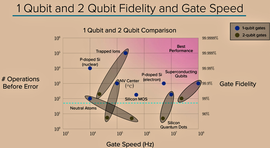
Figure 1.33: 1-Qubit and 2-Qubit fidelity and gate speed

Figure 1.34: 1-Qubit and 2-Qubit fidelity and gate error

1.39   The Promise of Quantum Computers

we have discussed how a quantum computer differs from a classical computer, and we have seen examples of the tremendous potential of quantum computing. In this section, we will turn to a more practical question: How can one realize the promise of quantum computing and quantum communication? Let us begin with the promise of quantum computation.

In this section, we will look at quantum algorithms and quantum communication. We will start by considering the promise of these technologies, what is needed to realize that promise, how to get there, and where we are today. Let us begin with quantum algorithms and the promise of quantum computers. As we discussed earlier, quantum computers are not smaller, faster versions of classical computers, nor are they an incremental step in the evolution of Moore’s law. Instead, quantum computing represents a fundamentally new approach to processing information. Furthermore, it is the only computing model we know of today. That is qualitatively different from existing computers. This difference and the potential promise of a quantum computer is reflected in the fact that simulating a quantum computer using a classical computer requires exponential overhead. This means that, as we add one qubit to the quantum computer, the size of the classical computer required to simulate it will grow exponentially. Now we do not often experience exponential growth in the everyday lives, and so, to gain an intuition for how powerful it can be, we may remember the old riddle where our employer asks us how we would like to be paid this month, and we have two choices. Either We will start us with one penny, and then each day for one month, We will double the number of pennies and keep the pennies from the last day. Alternatively, we can have $1 million. Now, it is entirely reasonable to think through the first few days of pennies. For example, two pennies on day one, four pennies on day two, double that to eight pennies on day three. Moreover, we begin to think that $1 million is starting to look pretty good. However, in fact, if we take that $1 million, we have lost a lot of money because the number of pennies is growing exponentially as 2 to the n-th power, where n is the number of days. So, on the 31st day, the last day of the month, we have 2 to the 31 pennies. That is equivalent to about $21 million. That is the power of exponential growth. Returning to computing, if we consider the amount of memory, we would need to store all the available states in the state space of a quantum computer We will similarly see the immensity of exponential growth. For example, representing all the quantum states of just 30 qubits would require at least a very powerful laptop. Increase that to just 40 qubits, and now we need a supercomputer. Double that to just 80 qubits, and we would need all the classical computers we have on Earth. Then double that again to 160 qubits, and now we need all the silicon atoms on Earth. Even small increases in qubits translate to exponential growth in the amount of memory required to represent all 2 to the n numbers that n qubits can store. So, there is a big difference between classical and quantum computers. Furthermore, this suggests the potential for substantial quantum advantage. However, what is needed to realize this in practice? To realize a quantum advantage, we need to identify the intersection of three essential requirements. First, we would like to identify a useful problem, one that has practical importance. Second, this problem should not have a known fast classical algorithm to solve it. Otherwise, we might as well just use a classical computer. Then third, the problem must have a known fast quantum algorithm, one that offers a substantial speedup. Now, this sounds great, but in fact, this promise has been mostly empty, except for a small area of overlap that we know about today. Nonetheless, there are useful problems with a quantum advantage, and this improvement can be quantified using a mathematical expression. One place is in the prefactor of that expression [180], and one place is in the exponential. The prefactor A can be a large fixed number, or it can scale polynomials with the number of qubits n. The exponential scaling of a problem of size n is in the exponential factor. Either of these two types of improvement can indicate quantum advantage. In the following sections, we will compare several algorithms and their respective speedup.

In the section above, an example of the power of exponential growth. In the salary example, if we earn two pennies on the first day, and double that amount each day for 31 days, then we will receive $2^{31}$ pennies on the last day of the month, equivalent to over $ 21M dollars. This growth rate is termed exponential because the output $y=2^{x}$ depends exponentially on the number of inputs x (in this case, the number of days). In computer science, algorithms can be classified according to the scaling of the resources required to run an algorithm as the number of inputs the problem size grows. An algorithm is said to scale exponentially if the resources (time, space) needed to run the algorithm grow following an expression such as $y=c^{x}$, where c is a constant greater than 1 and x is the problem size. Two other examples of growth functions are linear and polynomial. An algorithm is said to be linear if it can be solved by using$y=ax$resources, where a is a constant, and polynomial if it uses $y=ax^{c}$ resources where c is a constant greater than or equal to 1. The linear case is itself an example of polynomial scaling with $y=c=1$.

1.40   Understanding Quantum Algorithms

Realizing the promise of quantum computing relies on developing new quantum algorithms that offer a quantum advantage. In this section, we will review several algorithms that are known today and present several different approaches to the development of new quantum algorithms.

In the last section, the promise of quantum computing and its potential for quantum advantage. However, although a quantum computer can do anything a classical computer can do, it often does not improve. we only have a small set of useful algorithms at the disposal today. So, what can we do to realize the promise of quantum computing? Quantum advantage starts with having useful quantum algorithms. Developing new algorithms is very challenging, in large part because quantum computers are based on quantum mechanics. Thus, developing an algorithm for a quantum computer is quite different from doing so on a classical computer. To understand how quantum algorithms work and what they can do. There are currently a couple of different approaches. One is to develop algorithms based on mathematical theorems and their proofs. Shor’s algorithm and Grover’s algorithm are both excellent examples. Based on either intuition or insight into the problem, a quantum algorithm is first proposed. then, it is theoretically determined if the algorithm is efficient or not. For example, proving that an N-bit number can be factored with high probability, in a time that scales polynomials with the size of that and that N-bit number, rather than exponentially. Again, this type of development generally requires insight into a structure of the problem, that lends itself to enhancement on a quantum computer. A second approach is to use classical computers to simulate quantum computers’ behavior, to glean some insight into algorithmic primitives that can then be used to realize quantum enhancement in larger systems. Now, as we might imagine, simulating a quantum computer with a classical computer is not very efficient. After all, if we could easily simulate a quantum computer, we would not need to build one. Currently, classical supercomputers, with significant effort, can simulate about 50 qubits. Various probabilistic and Monte-Carlo techniques have been developed to further increase the qubit number, in exchange for accuracy or completeness in the solution. Again, these kinds of classical simulations can provide insights into how a quantum algorithm works at small scales[181]. So, it can be leveraged in quantum algorithms run on larger scale quantum computers. Beyond small scale simulations, a third approach is just to throw caution to the wind, build a quantum system, and see what happens. The D-Wave system is a great example of this approach. D-Wave has built a quantum annealer with more than 2000 qubits [182], a fantastic engineering achievement[128]. Although there is, yet, no theoretical or experimental evidence pointing to quantum enhancement in quantum annealers, at least for machines and problems studied so far, there remains a lot that we do not know. as we discussed previously, because optimization problems are so important, there is a tremendous application pull to develop quantum-enhanced optimization tools[183]. Thus, getting a real machine into the hands of engineers, computer scientists, and algorithm designers is a great way to start discussing what is and is not possible with the various quantum computing approaches. So, developing quantum algorithms is very challenging, and tremendous efforts have been applied to their development. it is because of this that we have useful, or potentially useful, algorithms today. Examples in the user now category are Shor’s factoring algorithm [184]and Grover’s search algorithm. Shor’s algorithm can be used to break public-key cryptosystems and afford exponential speedup over known classical algorithms. Doing so at a meaningful scale requires a medium-sized quantum computer, with thousands of logical qubits [185]. Although we do not have such quantum computers yet, they are foreseeable. research today is oriented towards developing new, quantum-resistant public-key cryptography standards, as well as a new generation of quantum algorithms to break them. Grover’s algorithm is related to a general class of search, collision, and optimization algorithms that afford a quantum advantage over known classical algorithms [186]. However, currently, more research is needed to help make these algorithms practical. There are a couple of reasons for this. One is the data loading problem. For example, we can efficiently load large amounts of data into a quantum computer so it can be efficiently searched. Also, there is currently a rather limited range of problem sizes that admit benefit. Namely, problems that are large enough to make use of the quantum advantage, and yet not so large that it becomes practically prohibitive to operate on a human time scale. For example, a quantum enhancement that reduces the runtime from a few thousand years to a few decades is obviously a fantastic improvement. However, very few people would find that useful. Although Shor’s and Grover’s algorithms are perhaps the most well-known examples of a quantum algorithm, it is widely anticipated that quantum simulation will have the greatest economic impact in the future. The simulation would apply broadly to a range of problems, from solid-state and nuclear physics to material science and chemistry. these are problems of importance to both science and industry. Classical simulations of quantum systems are generally limited to very small problem sizes, or an array of simplifying assumptions, such as no entanglement, or semi-classical dynamics[181]. Exact solutions are generally intractable because the number of variables needed to describe a fully quantum system grows exponentially with the problem size. It has been shown that quantum simulations can efficiently model quantum systems. the hope is that some of these problems may see the quantum advantage, on a smaller scale, or even error-prone quantum computers. Whether or not this is achievable remains an open question. Other quantum algorithms in the “may be useful" category include sampling solutions to linear equations [89], adiabatic optimization problems, and machine learning[187]. In these cases, the ultimate degree of quantum advantage will depend on several factors, including input-output complexity, such as the loading problem. We mentioned earlier and making a meaningful connection to applications. Besides, to offer a useful advantage, these algorithms must also outperform existing heuristics. Classical computing methods that, while not guaranteed to give an exact or optimal answer, do give very high-quality solutions. That is often enough for many applications. In summary, developing quantum algorithms that exhibit quantum advantage is at the heart of realizing the promise of a quantum computer. in the next section, we will look at the degree and type of quantum enhancement these algorithms provide. In the context of D-Wave quantum annealing versus gate model quantum computing[188, 189]. so, what is the potential of D-Wave’s quantum annealing machine versus, IBM or others’ quantum gate machines? And more specifically, which model will be a better choice for businesses in the immediate future? The universal gate model machines we know if we can build and engineer that system, there are problems that will have a quantum advantage when run on a quantum computer. But to get to that point requires fault tolerance and error correction. Now, in contrast to that, a quantum annealer addresses specifically classical optimization problems. it is not theoretically known whether a quantum annealer will afford quantum advantage or not over classical computers. There is no theory that says it will, nor is there a theory that says that it cannot. so, that is an open question. Now, it is true that there are many, many problems that can be broken down into optimization problems. Optimization problems are ubiquitous [190]. so, there is a huge application pull to develop computers, whatever they may be, that can solve optimization problems better than we can currently do. that is really the motivation for quantum annealing[191, 192]. we simply do not know if There is going to be quantum advantage there. Now, it could be that a quantum annealer is just a much better classical computer. if that is the case, it still has value. we think we still hope that There is a region of the parameter space where quantum annealers do show quantum enhancement. What we can say is that the quantum annealing in particular, the system that the D-Wave company has built, is really a fantastic engineering achievement. They very quickly, over a decade, went from just a few qubits up to systems with more than 2,000 qubits. They co-locate cryogenic electronics to control that machine. That is a fantastic achievement. But as a system engineer will know that to do that, they had to restrict the flexibility of that machine to a degree that it can scale quickly to those large sizes. so, the reason we bring that up is that there is some hope that, even though quantum enhancement has not been observed yet for a general class of problems the phase space that has been tested so, far is rather narrow. For example, only zz-type coupling interactions have been demonstrated. The degree of connectivity is limited to one specific type. the coherence times of the qubits that are used in the D-Wave machine are rather low when compared to the coherence times that we have on gate model machines. so, by moving to different types of coupling for example, xx-or yy-, sometimes called non-stochastic type couplings or to moving towards much higher coherence qubits, there is a hope that this may actually be a region of parameter space where quantum enhancement can be found.

1.41   Quantum Advantage

In this section, we will compare the resource scaling for several algorithms when implemented on a classical computer and a quantum computer. An improvement (reduction) in the resource-scaling is a quantifiable metric for the degree of quantum advantage.

In the last section, we introduced several algorithms, including those like Shor’s and Grover’s algorithm, that are useful now if we can build a quantum computer that is large enough and robust enough to run the algorithm. We also looked at quantum simulation, a very promising set of algorithms which, when realized, has the potential for substantial economic impact, and may even find utility on today’s smaller scale, non-error-corrected machines. we looked at a few potentially useful algorithms currently under development. For each of these examples, let us now look at the resource requirements for implementing an algorithm on both a classical and a quantum computer. It will then show the degree of quantum advantage one can obtain by using the quantum computer. We will also identify the leading limitations as They are currently known for realizing this advantage. Let us take them in order of their applicability as we see it today. At the top of the list is a quantum simulation[193] with application to quantum chemistry and material science[194, 195]. The classical resources scale as $2^{N}$-th power for simulation of N atoms, whereas the quantum resources scale as N to a constant power C, where C generally ranges from 2 to 6. Now, by resources, we mean both the time required to reach a solution, referred to as a temporal resource, and the number of logic or memory elements needed to implement the problem, often referred to as a spatial resource. To quantify the resource requirements, we quote a mathematical expression for the scaling law. We are looking at how the resource requirements grow as the problem gets larger, as parameterized by the size N, for example, the number of atoms being simulated. Presumably, as N gets larger, the problem gets harder. However, the question is, how does it get harder? Does it require exponentially more resources, such as $2^{N}$-th power, or a polynomial scaling, like N to an integer power? For quantum simulation, we see that the classical resources scale exponentially with N, whereas the quantum resources only scale polynomials. It means that there is an exponential advantage to using a quantum computer. To simulate the system dynamics for a time $t$, both a classical and a quantum computer would require a similar number of time steps. For example, if we want to simulate the dynamics of a reaction for one second, we would divide it into a similar number of time slices. However, the quantum advantage is that there is an exponential reduction in the amount of memory needed to perform the simulation on a quantum computer. Thus, the quantum advantage is exponential. The main limitation is in determining the mapping of a physical problem onto the qubits, their couplings, and the gate operations needed to implement a quantum simulation. Next, factoring and related number-theoretic algorithms also have an exponential scaling in the number of classical resources, going as 2 to the n-th power and the number of digits being processed. In contrast, the quantum resource requirements scale polynomial, as N to the third power. Thus, the quantum advantage is again exponential. The main limitation, or perhaps uncertainty, is that the best-known classical algorithm has not been proven to be optimal. So, there may still be a more efficient classical algorithm yet to be discovered[196]. if so, then the degree of quantum advantage might also change. Sampling solutions to linear systems of equations [197] is the next algorithm. In this case, we solve linear algebraic problems of the type $ax=b$, where $a$ is matrix, $b$ is a known vector, and $x$ is an unknown vector. The classical resources scale exponentially as $2^{N}$-th power, whereas the quantum resources scale only approximately as $N$. so, this algorithm also exhibits exponential advantage. The main limitation is related to a variety of restrictions on operating conditions. For example, a requirement for a sparse matrix A. The classical resources required for optimization problems also scale exponentially, as $2^{N}$-th power, where $N$ is again related to the size of the problem. However, in this case, the corresponding quantum resources, and the quantum advantage, are not well-defined. It is in part because one generally cannot determine if the resulting answer is indeed optimal. We can only tell if it is better than a solution We have had previously. Thus, we can only derive empirical evidence that a quantum optimization algorithm provides a quantum advantage. this is currently the main limitation of this algorithm. Finally, there is Grover’s search algorithm for unsorted or unstructured data. Here, the scale of the classical resources with the number of data elements $N$, whereas the quantum resources go as the $\sqrt{N}$. Thus, the quantum advantage is the $\sqrt{N}$, a polynomial enhancement. The main limitation of this type of search algorithm is the data loading problem. Namely, how can we efficiently load in a large amount of unsorted or unstructured data that needs to be searched? In general, we can see that, for many, if not all these algorithms, there can be a substantial quantum advantage when the problem size $N$ becomes large. for those with an exponential advantage, classical computers, and Moore’s law-like scaling will never be able to catch a quantum computer’s performance [198].

Developing applications that demonstrate a clear quantum advantage is challenging. However, there are several areas where the quantum advantage is known to exist (if we can build a large enough quantum computer to run the problem at scale).
Simulation of quantum systems: Quantum simulations of quantum systems afford an exponential advantage in the amount of space (memory) over classical simulations. Essentially, quantum systems generally comprise a very large number of variables to monitor during a simulation, and these can be handled more efficiently on a quantum computer.
Shor’s factoring algorithm: has an exponential temporal advantage over the fastest known classical algorithm for factoring. While it has not been formally proven that an efficient classical algorithm does not exist, it is believed that it does not.
Linear systems of equations: An exponential quantum advantage has been proven for linear systems that satisfy certain properties. From a matrix A and a vector b, the quantum algorithm can find a vector x such that $Ax=b$ as long as A is sparse and has a low condition number.
Grover’s search algorithm: has a proven polynomial speedup over the best possible classical search algorithms. This advantage is still subject to the data loading problem: the data to be searched must also be loaded into the quantum computer efficiently. Overcoming this loading problem is an active area of research.

It is challenging to prove that a quantum computer offers a quantum speedup for optimization problems. There are two main reasons for this. First, although one can generally identify a candidate solution and confirm that it is better than a previous solution, knowing (or proving) that the solution is optimal is generally not possible. Second, near-optimal solutions are often sufficient in practice for most problems. For example, in finding the shortest route home over a distance measured in kilometers, solutions that differ by a few meters are practically interchangeable with the true optimal solution. Proving speedup is thus confounded with the notion of “good enough,” making such proofs challenging. There is currently intense research to find quantum algorithms that provide a quantum advantage for finding higher-quality solutions in less time than is possible on a classical computer.

The following table compares the resource scaling for several algorithms that feature a quantum advantage. The resource scaling with system size N is shown for both classical and quantum versions of the algorithm when performed on a classical and quantum computing. The resulting degree of quantum advantage is shown along with current known limitations to the quantum algorithm implementation.

Figure 1.35: Quantum Speedups

1.42   The Promise of Quantum Communication

Quantum communication is qualitatively different from classical communication. In this section, we will discuss the promise of quantum communication and how to realize this potential by looking at what criteria must be met to realize the quantum advantage.

Just as quantum mechanics can dramatically enhance the way we process information, it also has the potential to enhance the way we communicate information. So, in this section, let us look at the promise of quantum communication. Communication is broadly defined as the conveyance of information, and it encompasses sending that information as well as receiving it. It certainly refers to verbal communication between people as well as nonverbal forms such as written text and signatures. It often comes in an encoded form. For example, the digital zeros and ones that are created by sampling the voices on a cell phone or representing the words of an email that are then routed from one computer to another. Even information on a chip must be shuttled around, communicated between a processor and its memory. Moreover, this concept can be extended to include several spatially distributed computing nodes, all of which are available to attack a problem but must be coordinated and require communication between these different nodes. All of these are examples of classical communication. However, quantum communication is different, and it represents a fundamentally different means to encode, convey, and authenticate information. These differences and the potential promise of quantum communication are reflected in three basic facts or theorems. The first is that classical information encoded in qubits can be transmitted two times faster than by classical means. This is achieved using a concept known as superdense coding, and it is a provable quantum enhancement. Two bits of classical information can be transmitted using a single qubit when that qubit is part of an entangled pair of qubits called a Bell state[199, noauthor_big_nodate-1]. Now, two qubits, but We only needed to transmit one of them to send two classical bits. That is superdense coding. The second is that quantum bits cannot be copied or cloned. Moreover, it is, again, a provable consequence of quantum mechanics. Now, if We prepared a qubit in each state, we know that state and so We can prepare a second qubit in the same state. However, if We have a qubit in an unknown state, we cannot make an exact copy of it, and that is called the no-cloning theorem. The third fact is that attempts to intercept or measure quantum bits can be detected. The no-cloning theorem cannot duplicate those bits. Thus, an eavesdropper must measure in order to glean any information. Moreover, it is the measurement process that always leaves a signature that is detectable in some way. What is needed to leverage these three facts and realize the promise of quantum communication? To realize the quantum advantage, we need to identify problems at the intersection of three key applications. The first is to find a problem that can leverage the enhanced capacity to encode information that quantum mechanics enabled. Second, there are problems related to authentication—the ability to confirm an individual’s identity or the truth of an attribute. Furthermore, third are problems associated with collaboration, the collaboration between people or agents such as secret sharing or game theory[200]. For example, enhance means to auction or to vote without attribution. Alternatively, using quantum mechanics to verifiably share public goods in a way that avoids certain rational yet self-destructive tendencies such as the tragedy of the commons. Realizing the promise of quantum communication will require finding problems that exhibit quantum advantage. In the next section, we will look at several such problems.

Communication describes the conveyance of information between a sender and a receiver. Some familiar examples of classical communication include verbal or written language, encoded information transmitted from one location to another via smartphones or the internet, and fetch calls made by a classical processor to its memory unit. Classical communication beyond speaking or writing is generally mediated by classical states of light or electricity, incapable of assuming quantum superposition.

Alternatively, the field of quantum communication considers the advantages that can potentially be found by communicating via the transmission of quantum states. Such quantum communication is fundamentally different from classical communication with respect to encoding, conveying, and authenticating information. These differences, and the potential promise of quantum communication, are reflected in the following three basic concepts.

The first concept is called superdense coding, also referred to as quantum dense coding (QDC). QDC is a fundamental quantum communications protocol that conveys two bits of classical information through the transmission of a single qubit. This protocol makes use of quantum entanglement as a resource and requires that the two users[201], traditionally referred to as Alice and Bob, have access to pre-shared entangled qubits.

As an overview, the protocol presumes that Alice and Bob have already pre-shared entangled qubits, such that each has one qubit from an entangled pair. Alice wants to send information to Bob, and so she proceeds to encode her information by performing one of four operations to the qubit in her possession. She then sends this qubit to Bob, so that Bob now has both entangled qubits. Bob then performs a joint measurement on each of the qubits now in his possession. By doing this, he is able to determine which of the four operations Alice performed during the encoding phase, and hence reveal two bits of classical information (since $\log_{2}(4)=2)$. Thus, Alice manipulates and sends one qubit to Bob, and in doing so, effectively transmits two classical bits of information.

The important feature of quantum mechanics, which enables this protocol to work, is the presence of entanglement, which provides access to a larger space of possible states. More specifically, if Alice and Bob did not share entanglement between their qubits, then the most information Alice could encode on the qubit she transmits to Bob is $\log_{2}=1$ bit, since the state space is spanned by two orthogonal states (usually written as $|0\rangle$ and $|1\rangle)$ it would just be a single, classical bit. However, due to the nonlocal nature of entanglement, Alice can hold just one of the two entangled qubits and still have access to the larger state space of the entangled qubits one that is spanned by the four orthogonal Bell states. Whichever Bell state Alice and Bob initially shared, Alice can change it to any of the other four through the application of one of the four following unitary operations to her local qubit: Identity, X-gate, Y-gate, or Z-gate.

To see how this works, Let us look at the four distinct Bell states for qubits A and B and label each with a unique binary number (00, 01, 10, 11):

$$\begin{split}\lvert\Phi^{+}\rangle&=\frac{1}{\sqrt{2}}\left(\lvert 0\rangle_{A}\lvert 0\rangle_{B}+\lvert 1\rangle_{A}\lvert 1\rangle_{B}\right)\leavevmode\nobreak\ \leavevmode\nobreak\ \leavevmode\nobreak\ \rightarrow\leavevmode\nobreak\ \leavevmode\nobreak\ \leavevmode\nobreak\ 00\\ \lvert\Phi^{-}\rangle&=\frac{1}{\sqrt{2}}\left(\lvert 0\rangle_{A}\lvert 0\rangle_{B}-\lvert 1\rangle_{A}\lvert 1\rangle_{B}\right)\leavevmode\nobreak\ \leavevmode\nobreak\ \leavevmode\nobreak\ \rightarrow\leavevmode\nobreak\ \leavevmode\nobreak\ \leavevmode\nobreak\ 01\\ \lvert\Psi^{+}\rangle&=\frac{1}{\sqrt{2}}\left(\lvert 0\rangle_{A}\lvert 1\rangle_{B}+\lvert 1\rangle_{A}\lvert 0\rangle_{B}\right)\leavevmode\nobreak\ \leavevmode\nobreak\ \leavevmode\nobreak\ \rightarrow\leavevmode\nobreak\ \leavevmode\nobreak\ \leavevmode\nobreak\ 10\\ \lvert\Psi^{-}\rangle&=\frac{1}{\sqrt{2}}\left(\lvert 0\rangle_{A}\lvert 1\rangle_{B}-\lvert 1\rangle_{A}\lvert 0\rangle_{B}\right)\leavevmode\nobreak\ \leavevmode\nobreak\ \leavevmode\nobreak\ \rightarrow\leavevmode\nobreak\ \leavevmode\nobreak\ \leavevmode\nobreak\ 11\end{split}$$ (1.37)

As an example, we assume that Alice and Bob initially share a $|\Phi^{+}\rangle$ state. If Alice wishes to send 00, then she need only send her qubit to Bob (the Identity operation). However, if Alice wishes to send the bits 10, then she must first perform an X-gate on her qubit, indicated with the subscript;
$A:(X\otimes I)\lvert\Phi^{+}\rangle=\frac{1}{\sqrt{2}}\left(\lvert 0\rangle_{A}\lvert 1\rangle_{B}+\lvert 1\rangle_{A}\lvert 0\rangle_{B}\right)=|\Psi^{+}\rangle$, with similar relations for the $Y-$ and $Z-$ gates. Once the encoding is complete, Alice transmits her qubit to Bob. With possession of both qubits, Bob is able to perform a measurement known as a Bell-state measurement. This measurement allows him to determine which of the four Bell states the two qubits are in, so he can decode the message.

While QDC offers a simple, clear indication of how classical and quantum communications differ, there are several important challenges to its real-world implementation. The first is that distributing a Bell state between distant users, a requirement to begin QDC is not trivial in practice. One of the most promising methods currently for this is to use photons entangled in such degrees of freedom as polarization, frequency, or time of arrival. Unfortunately, a single photon is extremely fragile. Therefore, it is likely to be corrupted or lost during transmission through free-space or optical fiber over distances of tens or hundreds of kilometers. A second challenge is how to store those pre-shared entangled photons before they are needed for communication. A third challenge is that the most straightforward ways to perform Bell-state measurements as currently do not distinguish between all four Bell states. For example, a setup might not be able to distinguish between the $|\Psi^{\pm}\rangle$ states, and hence only $\log_{2}$ (3) bits are conveyed with a single qubit. For these reasons, the rate at which information can be conveyed using QDC is at present significantly less than the rate at which classical communication can be performed in practice, making QDC an important protocol to study from a theoretical perspective, but unlikely to be of practical use any time soon.

The second concept is the no-cloning theorem of quantum mechanics, which states that an arbitrary unknown quantum bit cannot be copied. This is a fundamental consequence of the linearity of quantum mechanics. It is important to stress that this theorem only applies to unknown quantum states, for if the state is known, it can be identically prepared over and over again. However, given a qubit in an unknown state, there is no means to copy it and end up with two qubits in the same unknown state. This concept has far-reaching consequences, one of the most direct of which is that quantum states used for quantum communication cannot be amplified, since an amplifier should essentially make many copies of a state and sends them along the transmission path to amplify the signal. Efforts to overcome this limitation have resulted in significant research into what are called quantum repeaters. These devices potentially enable longer distance transmission of quantum states, but at a heavy technological price.

The third concept is that attempts to intercept or measure a quantum state are detectable, a pillar of secure quantum communication. The no-cloning theorem rules out duplication of an unknown qubit state. Therefore, a potential eavesdropper has no choice but to measure some aspect of a qubit to glean its information, and this measurement process always leaves a detectable signature. A sender and receiver, therefore, know when an eavesdropper is present.

Quantum communication holds the potential for quantum advantage. This promise is found at the intersection of three broad applications: source authentication, secure communication, and collaboration, each of which will be described in the next section.

1.43   Understanding Quantum Communication

The quantum advantage potential for quantum communication can be understood in the context of the number of participating parties, from two-user communication to multi-user distributed applications. In this section, we will discuss several such examples that illustrate the promise of quantum communication.

In the last section, we discussed the promise of quantum communication and its potential for quantum advantage. That advantage was based on three tenets of quantum mechanics, namely quantum-enhanced channel capacity, a concept known as superdense coding, the no-cloning theorem, which forbids copying an unknown quantum state, and a form of communication non-disturbance, by which any attempt to intercept or measure quantum bits can be detected. We can begin to understand how these tenets enable the promise of quantum communication by considering the number of participants as simultaneously participating in that quantum communication. The first example is the point to point secure communication using quantum key distribution. Secure communication relies on the use of a private key, essentially a string of bits used by a cryptographic algorithm. Quantum key distribution provides a means to transmit and share such a secret key securely. The secret key can then be used to encrypt and decrypt information. Any attempt to intercept that key can be detected, and when this happens, the compromised bits are simply discarded and replaced with additional secure bits. In this way, quantum mechanics enables two parties to communicate securely. Besides, We will discuss later, and quantum mechanics can also be used to generate true randomness, a resource for many cryptographic applications, and a step above existing classical pseudo-random number generators. Second are applications involving a few participants. One important example is quantum secret sharing amongst two or more people. Let us say Alice wishes to send a secret to both Bob and Charlie. She would like them to learn that information simultaneously so that neither Bob nor Charlie can have an advantage over one another by learning the secret first. Using quantum communication to distribute an entangled state shared between Bob and Charlie, Alice has created a situation where Bob and Charlie must coordinate to uncover what that secret is. They can coordinate on an open classical channel, but quantum mechanics will ensure that they receive the information simultaneously. Finally, the third set of applications involves multiple distributed participants or multiple distributed computing nodes that, in concert, perform a quantum algorithm. One example is quantum scheduling, which uses Grover’s Algorithm to search for a time when n distributed people are available. Another example is related to distributed computing systems, such as the leader election problem. In this application, a unique leader or a master node must be chosen from amongst all the distributed computing nodes. In both cases, it is known that quantum communication and quantum computing together provide an advantage over classical approaches. Despite the promise and numerous examples of problems where quantum communication gives an advantage, there are only a few practical applications to date. One application that is available now, even commercialized[202], is quantum key distribution or QKD. In QKD schemes, Alice and Bob want to share a private key, and any attempts by Eve to intercept it can be detected. There are demonstrations of QKD using photons over 100 kilometers of optical fiber and even a demonstration of transmitting signals between two points on earth using satellite quantum communication [26]. QKD even serves as a foil to quantum codebreaking by Shor’s Algorithm. We have already discussed, Shor’s Algorithm can efficiently break RSA public key encryption. It is also efficient against Diffie-Hellman key exchange and elliptic curve cryptographic schemes. However, messages encrypted using a one-time pad are, in principle, secure. One-time pad schemes use each bit in a key only once and then discard it. They, therefore, need to be continually renewed, and this can be done securely with QKD. The main issue with QKD security is that, as with most cryptographic schemes, there are many channels for the attack. For example, one must generally control access to the hardware used to implement a QKD scheme[203]. Another limitation is signal attenuation. Classical communication links use repeaters to regenerate and amplify a signal. However, due to the no-cloning theorem, this is not straightforward with quantum communication. Instead, We will discuss later in the section, a quantum version of repeaters has been proposed that can effectively extend communication lengths using quantum teleportation and distributed entanglement[204]. In conjunction with quantum memory, distributed entanglement would enable a quantum communication link to be established[205]. Other applications that may be useful include quantum secret sharing, auctioning or voting without attribution, verifiable quantum digital signatures, and message authentication. For all these examples, developing robust protocols and hardware systems that are immune to compromise will be necessary to realize the promise of quantum communication schemes fully.

1.44   Fundamentals of Quantum Communication

1.44.1 Non-Cloning Theorem

The no-cloning theorem states that it is impossible to replicate with certainty an arbitrary quantum bit. We can illustrate this statement by trying to come up with an operator $\hat{U}_{clone}$ that can clone a qubit. Let us assume we have found a unitary operator $\hat{U}_{clone}$ that can clone single-qubit states $\lvert 0\rangle$ and $\lvert 1\rangle.$

$$\hat{U}_{clone}\lvert 0\rangle\rightarrow\lvert 0\rangle\lvert 0\rangle\leavevmode\nobreak\ \leavevmode\nobreak\ \leavevmode\nobreak\ \leavevmode\nobreak\ \leavevmode\nobreak\ \&\leavevmode\nobreak\ \leavevmode\nobreak\ \leavevmode\nobreak\ \leavevmode\nobreak\ \leavevmode\nobreak\ \hat{U}_{clone}\lvert 1\rangle\rightarrow\lvert 1\rangle\lvert 1\rangle$$ (1.38)

However, if we apply this to an equal superposition state, following the rules of linear algebra, we find:

$$\begin{split}\hat{U}_{clone}\left(\frac{1}{\sqrt{2}}(\lvert 0\rangle+\lvert 1\rangle)\right)\rightarrow\frac{1}{\sqrt{2}}(\lvert 0\rangle\lvert 0\rangle+\lvert 1\rangle\lvert 1\rangle)\\ \leavevmode\nobreak\ \leavevmode\nobreak\ \leavevmode\nobreak\ \leavevmode\nobreak\ \leavevmode\nobreak\ \leavevmode\nobreak\ \leavevmode\nobreak\ \leavevmode\nobreak\ \leavevmode\nobreak\ \leavevmode\nobreak\ \leavevmode\nobreak\ \leavevmode\nobreak\ \leavevmode\nobreak\ \leavevmode\nobreak\ \leavevmode\nobreak\ \leavevmode\nobreak\ \leavevmode\nobreak\ \leavevmode\nobreak\ \leavevmode\nobreak\ \leavevmode\nobreak\ \leavevmode\nobreak\ \leavevmode\nobreak\ \leavevmode\nobreak\ \leavevmode\nobreak\ \leavevmode\nobreak\ \leavevmode\nobreak\ \leavevmode\nobreak\ \leavevmode\nobreak\ \neq\left(\frac{1}{\sqrt{2}}(\lvert 0\rangle+\lvert 1\rangle)\right)\left(\frac{1}{\sqrt{2}}(\lvert 0\rangle+\lvert 1\rangle)\right)\end{split}$$ (1.39)

As this example suggests, it is impossible to define a $\hat{U}_{clone}$ that can clone any arbitrary quantum state. This is a consequence of linear algebra and the nature of quantum mechanics, and it is called the no-cloning theorem.

1.44.2 Non-Disturbance

Non-disturbance describes the subsequent alteration of a quantum state due to measurement. The measurement process projects the quantum state on a particular predefined basis and causes an identifiable change. This process can be illustrated using the Bloch sphere. Suppose our predefined measurement basis is the z-axis. A measurement of a qubit in a superposition state will project it onto the z-axis. The resulting quantum state after projection (aligned with the z-axis) differs from the original superposition state before the measurement (it was not aligned with the z-axis). To conclude, attempted measurements of an arbitrary quantum state alter the quantum state and are, therefore, detectable.

1.44.3 Quantum Key Distribution

Quantum Key Distribution (QKD) is a communication method that uses unique features of quantum mechanics to exchange a secret key to encrypt and decrypt messages securely. In the underlying case, the keys are generated via a quantum channel between two parties, Alice and Bob. The principles of non-disturbance enable the detection of potential eavesdroppers on their quantum channels[206]. If the measured level of anomalies in their quantum measurement is below a certain threshold, the key is considered secure. Once a secure key is generated, it can, in turn, be used to encode and securely transmit information. The method of generating a secure key using quantum mechanics is known as quantum key distribution.

1.45   Industry Perspective: Introduction

In this section, we will discuss several leading industrial and start-up efforts targeting quantum computing. To get the discussion started, we asked several baseline questions. First, what technological approach are we employing to realize quantum computers, and why? Second, what is the business application we have in mind for the quantum computing systems we are developing? Third, what are the major technical hurdles we are facing? Fourth, how will our approach contribute to the advancement of scientific knowledge? Furthermore, fifth, what other industries are either vertically or horizontally integrated with respect to our efforts? We also add in other perspectives and thoughts not captured in these questions. The results are very interesting and informative. Thus, with that brief introduction, let us discuss the major commercial players in quantum computing today.

1.46   Industry Perspective: IBM

So, if we want to make a qubit, first we must decide what kind of qubit we want to make at IBM, we like to use superconducting circuit qubits. So, as the name already suggests, it is a circuit approach to qubits, and we use many superconductors. the favorite superconductors here are niobium and aluminum. we also make them on the silicon wafers. So, there is much expertise that we have locally and how to process and make them on the silicon platform. one ingredient that all the different superconducting circuits share is a Josephson junction, which is a little bit of an unusual circuit element. However, the way we make it is, we have two pieces of superconductors that are very weakly coupled. We just separate two superconducting electrodes by a very thin tunnel barrier. That is just an insulating layer. it is like 1/1000 of a hair thick. So very thin. This Josephson junction behaves like a non-linear inductor, but then to make a qubit, we need a second element, a capacitor. we make like of regular linear capacitor out of superconducting material. Then, tying these two together gives us an LC resonator that can behave as a qubit if we tune the parameters correctly. So now we have a qubit. In order to make a useful qubit processor, then we need to tie these different qubits together. We use microwave buses to couple them. then lastly, we provide input and output through a readout resonator to each of the qubits that then couples to the outside. Right over here is one of the dilution refrigeration systems, which cool down the superconducting qubit devices. There are several different plates inside here, which all sit at different temperatures. That gets down to 15 millikelvins. That is colder than outer space itself. The sound we hear is a pulse 2 compressor, which essentially is pumping on a closed cycle of helium 4, which helps us get the system cold. We have much other equipment that we use in order to run the processors. So, there is a lot of microwave hardware, different passive components including filters and attenuators, and co-ax cables, which allow us to send the signals down to address the qubits and to read them out to us the controllability. This is a four-qubit package. We have a five-qubit device that is right now inside of the fridge, but the general idea for how we package up these devices and cool them down is the same. this is a printed circuit board to which we mount the qubit chips. we wire bond to them to connect to essentially these co-axial pins. These co-axial pins connect to cables inside the fridge, allowing us to send the signals down and take signals back and read them out. We are not going to have quantum computers in our pocket. We will have quantum systems in the cloud that we will be able to access. for many people, day-to-day basis, they may not even know that their information is coming from a quantum computer in the future. However, they would benefit from the value that quantum computers have created. By the time we have 50 qubits or so, that system no conventional classical computer, that We have ever built or could ever build, could emulate what that 50-qubit quantum system will have. we are going to see it in the years to come. A central question in general that one must answer here is considering the amount of effort and the challenge that it is to build a quantum computer, why do we want to do this? Moreover, the answer is that there are applications, or there are algorithms for which we know these algorithms vastly outperform their classical counterparts. So, we may be familiar with Shor’s factoring algorithm or Grover’s search and so forth, just to name a few. What is important to keep in mind here is that these algorithms require a universal fault-tolerant quantum computer[207, 208, 209, 210]. At the current stage, we are still quite off from that. Several challenges must be overcome. The hardware must improve. We must develop better error-correcting codes so that the demands of the hardware become less. Nevertheless, at the same time, there has been steady and considerable progress in the experiments, with increased coherence rates and increased gate fidelities. We now enter a regime where it becomes challenging for classical computers to simulate these devices. Now, once we build increasingly large devices, we can ask ourselves, well, if this device is hard to simulate, is there already something meaningful that We can do with this? Furthermore, this is the question of trying to find near-term applications for quantum computers. Considering that we do not have a fault-tolerant computer, we must start making some concessions. Number one is we are going to have to look at algorithms or heuristics that do not come with a clean analysis, as they do for the cases as mentioned above. The other thing is that we must develop algorithms that are closer to the hardware that we are working on. lastly, we must think about errors constantly while developing those algorithms. We are currently focusing on three areas of applications: quantum simulation, quantum heuristics for optimization, and machine learning with quantum computers. One must keep this dichotomy to near-term and long-term in mind because many of the current algorithms that have been developed rely on having a fault-tolerant quantum computer. here, it is the task or goal basically to develop applications that are more closely tailored to the actual hardware that we are dealing with. Work is being done to develop error-correcting codes for use with quantum computers. Does the IBM Cube use an error-correcting code, or does it perform computations on a best-effort basis? If it does, what are the error-correcting codes it uses? And how does it implement that? So, many groups, including IBM, but groups worldwide, are focused on developing and demonstrating error-detection and error-correcting codes. today, there have been, we would say, very small-scale demonstrations of error detection by IBM and Google delved. there has been some demonstrations of error detection and correction, for example, at Yale, again, on smaller scale systems. But if we are asking about the online quantum computer that IBM’s using today, the answer is that it does not use error correction, active error correction, in this sense. As we will discuss there is a hierarchy to an architecture for building a quantum computer. at the bottom of that architecture, are the physical qubits. those qubits are they are good. But they are faulty. They have error rates of $10^{-3}$, to $10^{-4}$. to really run a computation at scale for a period of a day 24 hours, let us say we really need error rates at $10^{-15}$, to $10^{-20}$. So, to achieve that, we need to do active error correction. But in between the hardware and the active error correction, there is another layer that is been developed. this is used by groups worldwide. this is called passive error suppression or error mitigation [209]. what this is, essentially, dynamical decoupling. by applying the same types of gates, single and two-qubit gates, mostly single-qubit gates, that we use to control and run an algorithm, control the computer and run an algorithm, those same gates can be used to mitigate certain types of errors basically, coherent errors, errors where we do not lose information to the environment, but the qubit is dephasing in some way. those types of errors can be mitigated using dynamical decoupling. so, by applying these pulses, mitigating these coherent errors[211], we can make the fundamental physical qubits last even longer. They have even better error rates. that is important because error correction then, active error correction, is very expensive. the better the qubits are to begin with, the less overhead one needs to implement full-op error correction. so, what we would say is that we are not doing active error correction today, generally. But what we are doing, we would say, quite broadly is doing this passive error suppression. we want to call it error correction. So, we will call it passive error suppression or error mitigation [212]. Another part is, what is the status of error-correcting code development as it pertains to trapped ion qubits and semiconducting qubits? just to reiterate, we think in both cases, these technologies or the researchers who are pursuing these technologies are first working on error detection. So, to perform error correction, we first have to identify if and when an error occurred and on which qubits. the magic of quantum error correction, is that through specially designed syndrome measurements, we can make measurements which do not project the quantum information that we are trying to preserve. But they project onto a space where that information we gather is was there an error or not. So, we never discuss, for example, whether the qubit was in state 0 or state 1. We discussed that there was a bit flip error and that a 0 became a 1 or 1 became a 0. we discussed which qubit it happened on. so, with that information, we can go back and flip the qubit back to its correct value. But we never discussed what the correct value was. We never discuss whether it was supposed to be a 0 or supposed to be a 1. We only discussed that a bit flip error occurred, and we should flip it back. So, that intuitively the type of or the way that error correction works and to do that, we first have to detect if there was an error. We have to perform a syndrome measurement. So, many groups are working on doing those syndrome measurements for different types of error-correcting codes. Some of them are relatively simple codes, such as the bit flip code or the phase flip code. Some of them are more mature codes, like the surface code [213]. So, the surface code[214], for example, requires what is called a wait for parity check [215]. researchers, are trying to demonstrate that detection with high efficiency. then once their detection is mastered, then we can run error correction. We can go back in and correct for those errors once we discuss where they are.

1.47   Industry Perspective: Google

As with any information technology, quantum computing requires an entire stack. So, we go from application software to programming environments, all the way down to the hardware that realizes the actual quantum operations. for the hardware, we are currently banking on superconducting qubits since it is a technology suite that is complete. Thus, we know how to initialize a qubit. We know how to manipulate a qubit, or several qubits, by gate operations. we know how to measure those qubits. we know to do all those operations with rather high fidelity. However, we also keep a keen eye on competing technologies, such as silicon qubits or topologically protected qubits. However, at this point, we feel good that with superconducting technology, We will be able to build a small error-corrected quantum computer. On the software side, the most natural way to offer users access to a quantum processor is through a cloud interface. For example, a superconducting qubit the processors, they sit in a refrigerator that keeps them at about 10 millikelvins. it is too bulky to put this under our desk. However, it is no problem to have those in a data center. we abstract this complexity away from the user by offering a cloud API through which we access these processors. the roadmap for developing applications looks as follows. We will first start by passing a waypoint, which is known as quantum supremacy. Quantum supremacy roughly means the point at which a quantum computer, or some quantum device, surpasses the equivalent available technology on classical computers or classical devices. We are particularly interested in computational quantum supremacy, which means that a quantum computer will surpass for a well-defined computational task what we can do with a state-of-the-art supercomputer and state of the art classical algorithms. We call it the way post because the quantum supremacy benchmark task is not necessarily tied to something useful. So, it is important to realize that once we have achieved quantum supremacy, we are not yet in the phase of error-corrected quantum computing. To do error correction, like in classical error correction, we need redundancy. Unfortunately, the ratio of physical qubits to logical qubits to have one well-protected logical qubit is very high. It is about 1,000 to one. So, in order to have 1,000 logical qubits, we would need about a million physical qubits. we are still several years away from that. So, about quantum supremacy. it says, it looks like quantum supremacy has not been proved yet. Why do we need to invest our resources in quantum technology-related projects now before quantum supremacy has been proven? we would say that the aspect of quantum computing that there is a quantum speed-up that would, if we could build that system, demonstrate quantum supremacy that has been proven mathematically, that there are problems for which a quantum computer, if and when we build it, will provide quantum speed-up. Now, this second part of that question related to quantum supremacy has not been demonstrated yet. we think that we are close. we will demonstrate on probably a computer on the order of 100 qubits a calculation of some type that cannot be efficiently simulated on a classical computer. we think that that will happen. that will be a concrete demonstration of a problem for which there is quantum supremacy [216, 217]. we think that will happen within a year or two. Many companies are focused on doing exactly that, which is making a demonstration of quantum supremacy. Now, will that be for a problem that is useful that we will then use in our company to solve some problem that we have? That remains to be seen. We do not know yet. It could be that quantum supremacy is first demonstrated on a problem which may be of importance to, fundamental physics. It may be a problem that demonstrates some aspect of physics, but still needs to be translated into a practical problem for businesses. But we think that the concept of quantum supremacy is much more important than that. The concept is that we have demonstrated, in a real physical system, this concept that there are tasks that a quantum computer can perform and come up with an answer, and we can check that It is the right answer, but that a classical computer just cannot do efficiently. it will be a concrete demonstration. Even though we know mathematically, we have proven that this should be the case and is the case, we think having that physical hardware and demonstrating it directly is important. Nevertheless, we are optimistic that there are several areas in which we can develop algorithms that can already do something useful before error correction. There are probably three applications that We would encourage investigation. One is the quantum simulation. So, this is simulating quantum systems that cannot be simulated by even the world’s biggest supercomputers. The second area would be on discrete optimization. So, this is optimizing very complicated optimization problems. the third is machine learning. In terms of verticals, the verticals that We have seen much interest in would be automotive, aerospace, chemistry, pharmaceuticals, and, more broadly, just defense. the reason why We would say that these are interesting, especially automotive and aerospace, is that both these kinds of industries have both complicated optimization problems, but they also have chemistry-related problems[218]. For example, accelerating the development of batteries for electric cars. Right now, there are many issues with the battery technology we use. For example, it uses a rare material, such as cobalt. So, the number of batteries with today’s technologies that we can build. It is estimated to be 80 to 90 million batteries only, and then all cobalt reserves are exhausted. So, we need to find alternatives. there are just a lot of areas within the electrochemistry of a battery that, with quantum simulation, we possibly can better understand and devise better materials. Quantum processors are finicky beasts. They are cooled to below outer space temperatures. they need to be robust against noise and any interference that happens. so, one of the biggest challenges is just isolating these systems and keeping them in their quantum state. There are two main sources of noise for the systems. there is coherent noise and incoherent noise. we work to reduce both through excellent fabrication, also through the control electronics and the readout as well. Also, scalability is a big challenge for these systems. We are operating in a 20 to the 50-qubit range today. We are looking to scale up to 1,000, eventually a million, qubits. we must invent new technologies as we hit each of those certain milestones. What gotten we to one or two or 10 qubits is not going to get us to 1,000. so that scalability with the packaging, the electronics, the control is key for us to build a system that can scale up to a large enough size that we can run error correction on these chips, which we need. We all know how important computers are in our lives. We think about quantum computing. We have made a change into a realm where the basic rules are different. So, we think understanding the power of quantum computing is important for science, in general. In recent years, everyone has been very hyped, for a good reason, about machine learning and artificial intelligence. people have also been very excited about the possibility of using quantum computers to speed up computation. So, there is a natural question, can we put these things together? Furthermore, to that end, we have personally been thinking about specific setups for quantum computers to run machine learning tasks. We hope that we will discover some areas in classical machine learning where the quantum computers’ additional power accelerates or speeds up the machine learning tasks or allows for more reliable predictions, or perhaps learns to learn with fewer data coming in. Another area, which We think is sort of an obvious approach to use quantum computers, is if our data itself is not classical. So, we all know we can store classical data, like images, on classical computers. However, if We gave us a quantum system and We just told we it was a quantum state, that cannot be represented by a long bit string. The quantum state is too complicated. But nonetheless, quantum states exist in nature. So, we could ask, if We presented a quantum state to a machine a quantum computer could it learn to distinguish some attribute of that state which a conventional computer could not do? Moreover, the conventional computer might not be able to do it because it cannot even accept the input. Alternatively, even if somehow or another, we can encode the input, the quantum computer is just more naturally inclined to be able to answer questions about quantum states. So, we think that is a whole other area for quantum machine learning[219], which needs to be explored. For more information about Google’s Quantum AI research,[220, 221, 222, 223].

1.48   Industry Perspective: Microsoft

Microsoft, are building a full quantum stack, and the approach we are taking harnessing topological qubits that perform longer or more complex computations at a lower cost and higher accuracy. What it allows us to do is store and process quantum information in a more protected way. It is stored in a topological state of matter, these Majorana quasiparticles. What remarkable is that it has built-in fault tolerance and error correction. The actual value of the qubit is stored in a joint parity state, say over a nanowire, where that state is stored across two wires to form a qubit. Moreover, the computation then occurs by moving these quasiparticles around one another. It becomes what we call a braid in space-time, and this braid in space-time is the actual computation. Now it turns out these braids can be implemented through measurement only. So, we do not ever move the quasiparticles, but we can do joint measurements of these quasiparticles, and through sequences of joint measurements, we can enact and implement quantum computation. So, while other quantum approaches have more qubits right now, by number, in the short term, right, we believe the topological approach will deliver orders of magnitude, better accuracy, and scalability in the long term. When We think about the first business application, we think about how We will bring quantum to Microsoft’s cloud, Azure, and allow it to be integrated directly with people and organizations, apps, data, and infrastructure that is already existing. Moreover, we see users in Azure using quantum in concert with advanced classical conventional processing and storage. A quantum system, it will be unlike any other system built to date, and there are a handful of challenges that we must address as we seek to scale this system up. One challenge is the development of a robust, scalable qubit. We have been working on that advancement, with the topological qubit. Another challenge as we work up the stack is the development of the control and readout platform. We have been developing a state-of-the-art cryogenic compute and control system that cools matter to the coldest temperatures inside this dilution refrigerator, while also using an extremely small amount of energy. Throughout this full-stack, then, as we work up even further, we also need software to enable programming the quantum system and to enable running an actual application on the quantum system. We are building out not only a quantum development kit that includes a quantum focus programming language called $Q\#$, but we are also building the full runtime environment for running and controlling the quantum system. Within this runtime, there are several challenges to address, everything from optimizing compilation, layout, and scheduling of the algorithm on the actual device. We must be able to tune and calibrate and verify that the qubits and the operations and the compute. Then, at the highest level, we also face the challenge of developing quantum applications. Quantum computing and quantum algorithms present fundamentally new programming and algorithm design paradigms. How do we get speedups over classical approaches with these new paradigms? How do we fundamentally unlock new ideas in computing? We think we are only scratching the surface in terms of the potential of quantum computers. We already believe that what We have done in quantum computing has contributed to scientific knowledge. In 2012, the team member, Leo Kouwenhoven, and his team in Delft, they demonstrated evidence of the Majorana quasiparticle that underlies the topological qubit. This is not only fundamentally new physics, that really pushes the frontier of the scientific knowledge, but it is also a giant step forward toward a qubit that enables scaling more efficiently. In addition, we think other areas have pushed the scientific knowledge forward. It is in the area of studying quantum methods, quantum algorithms, and quantum programs. So, we have been able to bring new ideas from quantum computing over to classical methods and algorithms and programs. In turn, this has resulted in not only improvements in quantum algorithms, but We have seen improvements in classical algorithms from learning about quantum algorithms. So, for example, we have discovered remarkable connections between synthesizing gate sequences for a quantum computer, like single-qubit rotation operations, decomposing those into a sequence of universal discrete single-qubit operations. We have discovered that there is a connection there with algebraic number theory, which enables proofs of previously opened conjectures. It is truly amazing that quantum computing has the potential to really revolutionize the world to solve problems that we really cannot imagine solving with conventional classical computing. This is a fundamental, game-changing work. It is so exciting to be a part of that.

1.49   Industry Perspective: IonQ

We use individual atoms as the quantum bits. These are atomic ions, they are charged. We hold them in a vacuum chamber, and They are away from any surface. They are not part of the solid. So, they are nearly perfectly isolated from the outside environment, and this makes them perfect quantum testbeds to do quantum operations, quantum gates and to build up a large-scale quantum computer. There have been many results over the last few decades on manipulating these individual atoms and making small scale entangled states, small algorithms. They have largely been demonstration experiments, and they exploit the beautiful coherence properties of individual atoms and that each qubit is the same as its neighbor. So, when these qubits are idle, their quantum memories are as perfect as we can get because They are individual atomic clocks. There are challenges in scaling the system up to go beyond 50 or so qubits would require some sophisticated control engineering to not only trap these ions in a single device but also to think about moving entanglement not only between that device but to another device that has as many qubits. The challenge now in the implementation of quantum computing is to invent and perfect the controller system around these ions. This means that we must develop laser systems and optical control systems to move information around. While it is a challenge and this is unconventional computer hardware, the big benefit of having optical controllers from the outside is that the system is entirely reconfigurable. That means that the atoms themselves are not wired together explicitly; we wire them from the outside. So, we can change the pattern of wiring between qubits, and this leads to great opportunities in the programmability of the quantum computer. One key challenge facing the entire quantum computing industry is finding near-term commercially viable applications. There are very well-known applications for large scale quantum computers. However, today we are focused on developing flexible and fully reprogrammable quantum systems to help drive this technology development. While we expect early applications to be those that map naturally to quantum processes, like quantum chemistry or material simulation, even if niche, these applications will help drive the technology development and will allow us to continue to attract top talent. One of the biggest hurdles for scaling trapped ion quantum computation to larger scales is the sophistication of the laser control that is needed to manipulate these qubits. Currently, we are using multiple channels of laser beams that are controlled by these acousto-optic modulators. Traditionally, these types of optics were constructed on a big optical table using individual optical components, as we would see in an atomic physics lab. As the system gets more sophisticated, the complexity of that optical system gets out of control and, therefore, leading to instabilities, meaning things drift over time, very difficult to service if something goes wrong or some parts of it get misaligned. Because it is so spread out over such a large area, it becomes very sensitive to environmental conditions, such as temperature, the humidity of the room. It turns out that there are significant advances in optical integration technologies that were mostly invented in other nearby industries, such as optical lithography, telecommunications where optics are used to send data signals very far away, and also imaging systems where people are building very large scale high-resolution images. So, we are starting to adopt the technological progress of these areas in these other fields to try to design the control systems for the qubits that are much more scalable, has a lot of multiplexity, and also stable with the precision that we need to control the qubits. So, the ultimate solution, we believe, is to modularize the system where we take a large-scale quantum computer and break them up into a large number of smaller modules, each containing a manageable number, on the order of 100 qubits. We then try to make sure that those modules can be manufactured in vast numbers with a more reliable and compact geometry. Then assemble many, many of those modules and connect them together using a quantum interface in the form of optical communication or photonic interfaces, and that is how we are going to build a large-scale system. We find most exciting is not just the development and continued optimization of well-known algorithms today and applications today, but especially the discovery of new solutions, new capabilities. While we are in the very early days of quantum computing, if the development of classical computing is any indication, it is going to be very exciting next 5, 10, even 50 years.

1.50   Industry Perspective: Rigetti

Rigetti Computing is a full-stack quantum computing company building hybrid quantum-classical computing solutions. So, let unpack both of those. On the full stack side, this means we do everything from making the own design software to making the own chips in the case, superconducting qubit chips. However, we are packaging them in fridges, building control electronics, building software on top, and building that all into a cloud-deployed quantum programming environment, which, for us, is called Forest. So that is the first part. The reason we make this integrated approach is that a lot of the stuff at each of the layers has already been developed in academia, and now the big challenge is to integrate them and engineer them at scale and for a lower cost. The second bit is that we build hybrid quantum-classical computers, and this is to recognize that we are not going to have big, perfect quantum computers in the next few years. We are going to have small, noisy ones. So that means we should not treat quantum computers as standalone devices, standalone compute. They are co-processors that work in concert with classical computing resources. So, a classical computer can do things like tune around the noise in the quantum programs, or to assemble an ensemble of short quantum programs into the answer to a larger algorithm. So, from the ground-up, we have built the control racks, the instruction set, the programming environments, all to work in this hybrid model[224]. So, we are building full-stack hybrid superconducting qubit systems. There are three sets of areas that we are most interested in beginning with. Those are quantum simulation, optimization, and machine learning. So fundamentally, in quantum simulation, it is because we have these quantum systems that we can apply all the techniques We have discussed in classical approaches to solving computational quantum chemistry and map them into how to do quantum programming for quantum simulation. Then in optimization and ML, it is a little more nascent, but there we are using the fact that we have, basically, a large linear algebra resource and trying to figure out how to sample and exploit from it. So, we are excited about both those areas of development. We think the most important business challenge is not something that affects just Rigetti Computing. It affects the whole industry, and it is education. If we must have a Ph.D. in quantum computing to build the technology or use the technology, this is never going to change the world. So, we need to figure out a way to make a new kind of community. It is a quantum computer engineering community, and there needs to be a shared corpus. There needs to be shared the basic content. The basic textbooks are still to be written for this quantum computer engineering community. We need to both do that on a technical level, and then translate that into something on the business side that people come to understand. One way to think about quantum computers is as a way of exploring this new reality that is out there. We have known about quantum physics for 110 years, and it is played its way subtly into how the technology works in a lot of ways, but we never really grasped it. A quantum computer is like a vessel that we can use to go into this new area of exploration to see what we can do with large, well-controlled quantum systems. That is a very, very fundamental question. On the one hand, if it turns out that we cannot build quantum computers, this would break the models of physics, which is almost as interesting as the stuff we can do by applying them in a powerful way. There is so much foundational stuff to do. There are so many foundational concepts to discover. There is just a lot of ways on how to create an impact on how the field will evolve and grow. There is just not a lot of historical opportunities to be at the forefront of something like that. It is like we are going back to the 50s or 60s and saying, this computing thing that might happen. How could we be involved in that? Furthermore, quantum computers can happen faster because we have all regular computing to help us.

1.51   Industry Perspective: QCI

We have been pioneering a couple of new approaches for how to make quantum computations more robust and more easily scalable. This is what we call hardware efficient error correction, which means we need fewer parts to build into our quantum computer. Something called the modular architecture, which is a way of assembling smaller pieces into a more powerful whole, entangles them. The machines we see in the lab, are used to cool the special superconducting quantum circuits to temperatures a few thousandths of a degree above absolute zero, where we can prolong their quantum behavior, and where all the elements inside become superconducting so that there is no electrical loss in the computer at all. There are several other players in this field, including Google and IBM. Moreover, they also use superconducting qubits and a circuit QED approach. They have decided to make their quantum processors out of a relatable technology, in the form of big 2D grids of these devices. QCI takes a different approach. We believe that just like supercomputers should be, and are, built out of networks of simple processors, quantum computers should not just be large grids of qubits. Thus, we are making the architecture modular, in the sense that the goal is to build a quantum computer out of reliable, easy to understand, and easily characterize units that are connected in a reconfigurable way. Thus, we feel we have a real head start, and a much easier path to rapidly scaling to large scale and useful quantum computers. What is special about the quantum system is that they offer possibilities that no classical system will ever offer. They operate on using, not the conventional logic we are used to, which is the Greek logic, but the logic of nature. There are aspects of it which we cannot predict as of now. We mean, there is an event and breakthrough that will make this new science available in fields that are not even thinkable as of now. So just a bit like asking the makers of the first classical vacuum tube computer to predict the internet.

1.52   Industry Perspective: D-Wave Systems

D-Wave uses superconductor integrated circuits to build annealing quantum computers. In terms of annealing quantum computing, this is kind of the most interesting part of what D-Wave has chosen to do because it is very different from what most of the quantum computing community has chosen to focus on, which is called gate model quantum computing. We are trying to harness quantum mechanical tunneling. So, the qubits have the possibility of tunneling back and forth between the zero and the one state. We can control how easy it is for them to tunnel back and forth between these two states. So, we start the algorithm, the quantum annealing algorithm, where all the qubits in the system are tuned so that it is easy to tunnel back and forth between zero and one. Furthermore, the idea with quantum annealing is to start in that configuration and progressively make it more difficult to tunnel back and forth between the zero and the one state. So, at the beginning of the algorithm, the system, each one of the qubits is in a superposition of zero. One and the system is, in a sense, in a superposition of all possible answers that the final processor could encode. Some of those answers in that superposition are going to be the better or best answers for our set of constraints. We just do not know which ones yet. The algorithm works because we start with our dimmer switch turned down in this way, and we gradually turn up the strength of the constraints that we wanted to program on the processor. We are stating the problem more and more strongly as we go. Moreover, as we are doing this, we are making it more and more difficult for the qubits to tunnel back and forth between the zero and the one-state—each of them. The idea with this, and again, just at sort of a hand-wavy level, is that we progressively select out, preferentially select out, those combinations of zeroes and ones, which are going to end up being the better answers. The lower energy cost-function answers out of this large massive superposition. Annealing quantum computing is relevant in areas of optimization, sampling, and machine learning. It cannot run Grover’s algorithm, which is a prescription for a gate model algorithm, but it naturally solves an optimization problem at its core. Everything in a superconducting integrated circuit is made with Josephson’s junctions. The current generations of processors have about 135,000 of those junctions on them. So, scaling the technology to be able to yield at that level has been challenging. However, also, the actual architecture of the processor to function, to be programmed, measured, and annealing properly at that kind of scale has been a big challenge. D-Wave has had to tackle the problem of bringing classical control circuitry directly into the quantum processors’ environment to control and manipulate them and read them out properly. However, we are not there yet. So, there is still is a little way to go to mature technology. There is a whole world in front of us. What we find are the major challenges still facing us are continuing to scale the processors and crossing into a territory where we can run real commercial applications. So, D-Wave was the first company to produce a commercial quantum computer. We are the first to be able to go through these rapid development cycles, get customer feedback. Then the physicists, engineers, and software developers can improve the architectures as sort of, as pointed by customers working on actual applications and making them better. People discuss, in the digital computing world, that Moore’s Law is coming to an end. In the part of the quantum computing market, we have gone from 120 qubits to 500 to 1000 to 2000, and then machines with four of five thousand qubits are on the horizon in the next few years as well.

1.53   Limits of Classical Computing: A Brief Introduction to Computational Complexity

We have discussed the promise of quantum computers and their potential for quantum advantage. Some problems are very hard to compute on a classical computer, and for some of these problems, a quantum computer is much more efficient. However, what makes a problem hard in the first place? we have probably discussed problems being categorized as $P$ or $NP$, $NP-$complete[225]. Nevertheless, what do these categories mean, and how do computer scientists classify a problem as an easy problem or a hard one? In this deep dive, We will discuss about the computational complexity of classical computing[84], how it is defined, and how problems are classified, including a discussion of several standard problems that are classified as $P$, and $NP$, and $NP-$complete. Let us describe a little bit about universality in the language of the circuit model of computation. That is what we naturally know best and is what we will build quantum computation upon as a language. So, in the circuit model, for example, we may have AND gates and NOT gates. we want to claim that all Boolean circuits, circuits that compute Boolean functions, can be composed of AND and NOT. this is easy to see, but first, let us look at the family of Boolean functions. They will be functions that take, if there are $n$ bits of input, say $x_{0}$ to $x_{n-1}$, and the result of this is going to be either 0 or 1, so for example, in the notation, We will say that we may have $f$ of $x_{1}x_{2}$ be $x_{1}x_{2}$. this product represents an AND gate. Alternatively, for example, $f$ of $x$ is equal to $\bar{x}$ . This is how we will represent a NOT gate? Now, the question of universality dovetails with another question. we have not finished the universality description yet. However, we want us to keep this in mind of complexity because it is not useful if We say something about universality without saying how much cost it takes to accomplish something. So, the key idea which we will not have time to go into much depth on, but We hope we already know something about, which is that some math problems are harder than others. we do not mean it is hard to multiply two million-digit numbers, and that is harder than multiplying two 10-digit numbers. No, that is not the point. The point is They are scaling with respect to the size of the problem. this leads to a statement which we hope that all of we already know of in some form, which is called the Strong Church-Turing Thesis. we will write this up for us because we think the words of this are instrumental in understanding the perspective. So, we say, any model of computation can be simulated on a specific kind of machine. the machine and model We would choose will be this one here, the Turing machine. However, we are going to choose a specific variant of it, the probabilistic Turing machine. we need to say something about the cost of this kind of simulation. the essence of that thesis is that this simulation cost comes with, at most, a polynomial increase in the number of elementary operations required. It is an excellent thesis. It defines equivalence between models, whether they be electrical and optical or electrical and DNA or quantum and DNA or quantum and classical. for even that to be possible, conceptually is remarkable. we have not defined a lot of the technical terms in this, like simulation and the overhead costs, but We hope we will appreciate that as we go along. So now, in order to highlight this statement of equivalence, let us make sure we are aware of one of the greatest motivating factors for quantum computing, which is the difference between two of the most important classes of mathematical problems. we will use this fact that many problems can be expressed as decision problems. So, for example, is the number $M$ prime? Furthermore, the answer to this is yes or no. Is this a hard problem or an easy problem? This was not known for many years. It was then realized that we could answer this question with some randomness. we would not know it for certain. This is Rabin’s primality testing algorithm. then some 15 years ago, somebody in India proved that we could do it deterministically. So, it moved from this probabilistic model, which people had to use previously for this question, to something which did not need probability. So today, there is a deterministic primality testing algorithm. This problem is called primality. That is one example. Here is another one. It is called factoring. Given a composite integer m, but not just the number that we are going to try to factor, also and a number l, an integer l, which is less than $m$, does $m$ have a factor that is non-trivial which is less than l? So, we need to bound the sides of the range of numbers we are going to consider as being answers to the problem. again, this is a yes or no question. we have this distinction. If the time taken to answer this question, needed to answer this question, it is polynomial in the size of the question. Here, for example, for factoring, this is the number of bits of $m$, the number of digits in the number, not just the number itself, then we say that the problem is polynomial in complexity. We say it is in this class that We will call $P$. Now, let us break down the class on whether this is answered by a yes or by a no. If the yes instances of the problem are easily checked, and We will use the word verified as a technical term with the aid of a witness, which is a short description piece of information that enables somebody else who is not skilled at the arts but can be very reliable, to verify our claim. Sometimes, we discuss Merlin and Arthur [226]. We say that the Merlin is very clever and can come up with proofs, but we need the Arthur, who is not clever but can be very, very reliable to take that proof and verify the claim. So, there are two parties to this, the verifier and the prover. the verifier takes this witness. If this is true, then the problem, even if it is challenging, is the fact that we can verify that the proof of it means we will say that the problem is in this class called $NP$. in some senses, we want to say this is non-polynomial, but the main point is the distinction between $P$ and $NP$. for the sake of completeness, we have another parallel to this: the mirror image. If no instances, so this is the answer is yes, and the answer is no with the same language, then we say that the problem is in a different class called $co-NP$. we do this not because We want to say anything more about P versus $co-NP$ or $NP$ versus $co-NP$, but just to share with we a trivial fact in a moment. So, the reason We show this is because so much of the motivation for computation today, and much of quantum computation comes from this question of $NP$ versus $P$. We think that the $P$ problems are easy. The $NP$ problems are the hard ones and meaningful ones to do. There is this plot that we can make, which shows that, if this is the space of all mathematical problems, then $P$ is a subset of something we might say is $NP$, but there is also this extra area over here, which is the hardest of the $NP$ problems. we call these $NP-$complete problems. they are defined as such because, if we can solve any of the $NP-$complete problems, then it gives us a polynomial-time algorithm to solve any other problems in the $NP$ regime. So, where is quantum computation in all this map? Well, we are not going to answer that for we today, but We hope that, through this, we will start to appreciate where quantum computation is relative to this landscape of the field of all problems and their complexities. Quantum computation sits a kind of difference in this landscape. It has a complexity class, typically of something we call $BQP$ [227, 228, 229]. part of the reason is that the model is slightly different and does not fit directly into either of these classes, because sometimes the output is quantum mechanical. There are errors involved, and some things We will come to later. Good. We hope that many of us already knew about most of this, but We also hope that it starts to connect some things for us. An example of an $NP-$complete problem and now We going to go back to the concept of universality is, so an example is a problem called $3-SAT$. this is about the satisfiability of Boolean functions, which looks something like this. So, suppose we have, again, a function of bits $x_{0}$ through $x_{n-1}$. The formulas that are involved in $3-SAT$ look something like $x_{1}+x_{3}+x_{9}$, OR’d together, AND’d with there is a multiplication here another term, like $x_{4}+\bar{x_{7}}+x_{11}$, and so forth and so on, where each one of these terms just has three bits. our goal is to say, does there exist an assignment of zeros and ones to the $x$ inputs such that the output is equal to 1? It seems very simple. It is straightforward to write this problem on the board. However, if we can solve this problem fast in time. That is polynomial with $n$ here, and then it turns out we can quickly solve all the rest of these problems. if we can solve this problem fast, we can solve problems like the optimum way to pack boxes into a FedEx truck, or the optimum way to route a packet in for information from San Francisco to Boston. we know, it is remarkable how powerful such a simple problem can be. However, we can show that, in practice, we cannot solve most of the instances of this problem as well as we would like to. Are there simple problems that are neither $P$ nor $NP$? Are there simple problems that are neither P nor NP? Another interesting class that sits outside of this class is counting the number of solutions to a problem. That is the class called sharp$-P$. so forth, because we might count the number of things to count the number. However, we know this is how we get a career as a theoretical computer scientist. It is very effective.

1.54   Computational Complexity: Topics on Complexity Theory

So, what is complexity theory? Theoretical computer scientists love to come up with complexity classes[230]. So, $P$ is polynomial-time computation. $NP$, things we can prove in polynomial time. So, who here does not know about $NP$? So let us explain $NP$ a little bit. The most famous $NP-$complete problem may be the traveling salesman problem. Here we have a graph, distances between, let us call them, cities, which are the nodes of the graph. The question, is there a path visiting all cities less than length l? So, this might be 1, 2, 3, 5, or no 2, 3, 1, 1, 2, 3. So this would be a path of length 12. Moreover, there are distances We mean there are roads between the cities. We have not put on here at distances along those roads. If these were the only roads, it would be an easy problem. If there are only six vertices, it is an easy problem. So, it is easy to prove. So, if We want to prove that there is a path, we just give us the path, and we add up the distances and check it. Moreover, we can prove it. However, it is hard, or it may be hard to prove no. So how can We prove that there is no path shorter than distance 12 on that route? We could run through all paths and check all their distances, but that takes a very long time. If We know, and if We were trying to convince us that we have done this, would there be a better way to convince us other than just say, well, we ran through all the paths and checked them? Furthermore, there are better ways for the traveling salesman problem, but they all seem to be an exponential time in the worst case. Or the exponential time in the number of cities. Now, some problems are $NP-$Complete, which is as hard as any $NP$ problem. In other words, if We could solve an $NP-$Complete the problem in polynomial time in the length of its input, we could solve any problem in $NP$ in polynomial time the length of its input. We do that by reducing one problem to another. Furthermore, at some point in the 1990s, we think computer scientists came up with interactive proofs. There are three classes of interactive proofs. $IP$, no bound on the number of rounds, $AM$, and here $``A"$ stands for Arthur, and $``M"$ stands for Merlin. Merlin has infinite computing power, and Arthur only has a polynomial amount of computing power. So, $A$ sends $M$ message, $M$ returns the message. So that is two rounds. Then there is also an $MA$. $M$ gives proof. $A$ verifies it with coin flips. So, $NP$, Merlin gives Arthur a proof, and Arthur verifies it deterministically. $MA$, Merlin gives Arthur a proof and Arthur verifies it, but probabilistically. Moreover, $AM$, Arthur sends Merlin a message, and Merlin returns a message. The classic example of $AM$ is graph non-isomorphism. Are these two graphs isomorphic and $NP$. We are given two graphs, and We guess these have 5, 6, 1, 2, 3, 4, 5 6. So, the question is, is there a way to relabel the vertices so that they are the same? Moreover, the guessed answer is an $NP$, and an isomorphism is in $NP$. Merlin just gives Arthur a relabeling. So, Merlin says 1 in this graph corresponds to 5 in this graph. 3 in this graph corresponds to 4 in this graph. Non-isomorphism is an $AM$. Arthur takes one of the graphs. He re-numbers the vertices at random, and he sends it to Merlin. Furthermore, Merlin is supposed to Merlin says which graph it is. Now, if the two graphs are isomorphic, we know, Merlin has the scrambled graph, but a random scrambling of this graph looks exactly like a random scrambling of this graph. So, he cannot tell them apart. If Merlin has an infinitely powerful computer, he can try all possible permutations and tell them apart if the two graphs are not isomorphic. So that says that non-isomorphism is an Arthur-Merlin.

1.55   Classical Circuit Model

This section we will program and execute the Deutsch-Jozsa algorithm on a cloud-based quantum computer using the IBM Quantum Experience[231]. The Deutsch-Jozsa algorithm is programmed and implemented using a quantum circuit model of quantum computation. To get started, let us first review an example of a circuit model for classical computation.

In this section, we will run an actual quantum algorithm, the Deutsch Jozsa algorithm, on a real quantum computer. Of the section, we will first discuss in detail how that works. To do this, we will need to introduce the algorithm using a circuit model of quantum computation [1]. However, before we do that, let us first examine a circuit model in the context of classical computation. The circuit model for classical computation begins with input data prepared at the initialization stage. We can think of the computational bits in the input register being reset to all zeros and then set to the initial values that will be input to the computer. Now, this reset step may not be necessary for a classical computer. However, we will include it here for comparison with the quantum circuit model that We will discuss later. The initialized bits are then inputted to a computational stage. Here, a series of logical operations are implemented using classical Boolean logic gates to compute a series of functions. Furthermore, once this is complete, the output for this stage encodes the result of the computation. For example, let us consider a full adder circuit comprising a series of Boolean logic gates. The full adder takes as inputs the bits B1 through B3. Where B1 and B2 are the binary numbers we want to add, and B3 holds any carry in that we may have from a previous calculation. Here we do not have a carry forward, so its value is zero. An output of this circuit is the sum, B1 plus B2 modulo 2, where the modulo 2 arises because this is binary arithmetic. The second output is the arithmetic carry out that may result from the addition. These two values are then assigned to bits B4 and B5 and stored in the output register. In this case, we add 1 plus 1, which is 2 with decimal numbers. Furthermore, for the binary addition performed by this circuit, the addition is modulo 2, 1 plus 1 equal 0, and has a carry forward of 1. Finally, the results from this addition problem are obtained in a measurement stage, where the values of bits B4 and B5 are the binary representation of the answer, which may then be converted back to a decimal result. This type of initialized, compute, and measure process is the foundation for a universal classical machine. To access this machine, a user interface provides the input data and the program instruction set to calculate the desired function. This instruction set is then applied to the physical hardware using a controller layer. This layer takes the input data, sets the input bits, implements the physical logic gates according to the instruction set, measures the output, and then sends the resulting data back to the user interface. This computational model illustrates the basic building blocks that we need to implement an algorithm using a quantum circuit model. The main distinction will be the role of quantum mechanics and its impact on the initialization, compute, and measurement stages.

The blueprint for implementing an algorithm on a classical computer is the classical circuit mode. It describes how a set of input states is manipulated by a processing core and subsequently stored in an output register.

For example, a 2-bit$\times$2-bit binary multiplier uses a series of Boolean logic gates to multiply two input numbers, each taking an integer value between 0 and 3. The computation starts by first resetting the input register and then initializing it to the values of the two inputs represented as binary numbers. After that, the input states are then processed by a gate sequence that implements multiplication. Finally, the resulting output bit sequence, the computed result is placed in the output register where it can be readout.

All possible 2-bit inputs (a and b) and resulting outputs (c) are summarized in the following table:

Table 1.1: 2-bit inputs (a and b) and resulting outputs (c)

decimal	binary	decimal output	binary composition	binary output
$a\cdot b$	$[a_{1}a_{0}]\cdot[b_{1}b_{0}]$	$c$	$c_{3}2^{3}+c_{2}2^{2}+c_{1}2^{1}+c_{0}2^{0}]$	$[c_{3}c_{2}c_{1}c_{0}]$
$0\cdot 0$	$(00)\cdot(00)$	$0$	$0\cdot 2^{3}+0\cdot 2^{2}+0\cdot 2^{1}+0\cdot 2^{0}$	$0000$
$0\cdot 1$	$(00)\cdot(01)$	$0$	$0\cdot 2^{3}+0\cdot 2^{2}+0\cdot 2^{1}+0\cdot 2^{0}$	$0000$
$0\cdot 2$	$(00)\cdot(10)$	$0$	$0\cdot 2^{3}+0\cdot 2^{2}+0\cdot 2^{1}+0\cdot 2^{0}$	$0000$
$0\cdot 3$	$(00)\cdot(11)$	$0$	$0\cdot 2^{3}+0\cdot 2^{2}+0\cdot 2^{1}+0\cdot 2^{0}$	$0000$
$1\cdot 0$	$(01)\cdot(00)$	$0$	$0\cdot 2^{3}+0\cdot 2^{2}+0\cdot 2^{1}+0\cdot 2^{0}$	$0000$
$2\cdot 0$	$(10)\cdot(00)$	$0$	$0\cdot 2^{3}+0\cdot 2^{2}+0\cdot 2^{1}+0\cdot 2^{0}$	$0000$
$3\cdot 0$	$(11)\cdot(00)$	$0$	$0\cdot 2^{3}+0\cdot 2^{2}+0\cdot 2^{1}+0\cdot 2^{0}$	$0000$
$1\cdot 1$	$(01)\cdot(01)$	$1$	$0\cdot 2^{3}+0\cdot 2^{2}+0\cdot 2^{1}+1\cdot 2^{0}$	$0001$
$1\cdot 2$	$(01)\cdot(10)$	$2$	$0\cdot 2^{3}+0\cdot 2^{2}+1\cdot 2^{1}+0\cdot 2^{0}$	$0010$
$2\cdot 1$	$(10)\cdot(01)$	$2$	$0\cdot 2^{3}+0\cdot 2^{2}+1\cdot 2^{1}+0\cdot 2^{0}$	$0010$
$1\cdot 3$	$(01)\cdot(11)$	$3$	$0\cdot 2^{3}+0\cdot 2^{2}+1\cdot 2^{1}+1\cdot 2^{0}$	$0011$
$3\cdot 1$	$(11)\cdot(01)$	$3$	$0\cdot 2^{3}+0\cdot 2^{2}+1\cdot 2^{1}+1\cdot 2^{0}$	$0011$
$2\cdot 2$	$(10)\cdot(10)$	$4$	$0\cdot 2^{3}+1\cdot 2^{2}+0\cdot 2^{1}+0\cdot 2^{0}$	$0100$
$2\cdot 3$	$(10)\cdot(11)$	$6$	$0\cdot 2^{3}+1\cdot 2^{2}+1\cdot 2^{1}+0\cdot 2^{0}$	$0110$
$3\cdot 2$	$(11)\cdot(10)$	$6$	$0\cdot 2^{3}+1\cdot 2^{2}+1\cdot 2^{1}+0\cdot 2^{0}$	$0110$
$3\cdot 3$	$(11)\cdot(11)$	$9$	$1\cdot 2^{3}+0\cdot 2^{2}+0\cdot 2^{1}+1\cdot 2^{0}$	$1001$

A 2-bit$\times$2-bit multiplier can be constructed using Boolean logic gates of the following type (note: this is not a unique construction):

AND gate: outputs logic-state 1 solely if both input bits are in logic state-1, and outputs 0 otherwise.

XOR gate: outputs logic-state 1 if the input bits differ, and outputs 0 otherwise.

Analyzing the output bits $c_{0}$ through $c_{3}$ yields the following conclusions:

• $c_{0}$ equals 1 only if both a and b are non-zero and odd. Therefore, an AND gate applied to the bits $a_{0}$ and $b_{0}$ is sufficient to compute $c_{0}$:
  $c_{0}=a_{0}\leavevmode\nobreak\ AND\leavevmode\nobreak\ b_{0}$

• $c_{1}$ will equal 1 if not all input bits and either $a_{0}$ and $b_{1}$ or $b_{0}$ and $a_{1}$ are in logic-state 1:
  $c_{1}=(a_{0}\leavevmode\nobreak\ AND\leavevmode\nobreak\ b_{1})\leavevmode\nobreak\ XOR\leavevmode\nobreak\ (a_{1}\leavevmode\nobreak\ AND\leavevmode\nobreak\ b_{0})$

• $c_{2}$ will equal 1 only if both primary bits $a_{1}$ and $b_{1}$ but not all involved bits are in logic-state 1:
  $c_{2}=((a_{0}\leavevmode\nobreak\ AND\leavevmode\nobreak\ b_{0})\leavevmode\nobreak\ AND\leavevmode\nobreak\ (a_{1}\leavevmode\nobreak\ AND\leavevmode\nobreak\ b_{1}))\leavevmode\nobreak\ XOR\leavevmode\nobreak\ (a_{1}\leavevmode\nobreak\ AND\leavevmode\nobreak\ b_{1})$

• $c_{3}$ equals 1 only if all bits composing a and b are initialized in logic state 1:
  $c_{3}=(a_{0}\leavevmode\nobreak\ AND\leavevmode\nobreak\ b_{0})\leavevmode\nobreak\ AND\leavevmode\nobreak\ (a_{1}\leavevmode\nobreak\ AND\leavevmode\nobreak\ b_{1})$

The result stored in the four-bit output register is obtained via a measurement of the register and, for the users convenience, can be converted back to a decimal result. The sequence of initialization, computation, and measurement summarizes the working principle of universal classical machines. Although universal quantum machines [232] follow the principles of quantum mechanics and therefore require a different approach for implementing individual computational steps, the concepts derived from the classical circuit models serve as the basis for designing quantum circuit models.

1.56   Quantum Circuit Model

In this section, we will discuss the quantum circuit model and its similarities and differences with the classical circuit model. The quantum circuit model applies to gate-model algorithms, such as the Deutsch-Jozsa algorithm that we will implement in the lab practicum.

In the last section, we introduced a circuit model for classical computation. This model included an initialization stage to set the input bits, and a compute stage that implemented classical logic gates to compute a function and a measurement stage of extracting the output. In this section, we will introduce an analogous circuit model for quantum computation. The basic structure is the same. Initialize, compute, and measure. We will start with an initialization stage where the qubits are first to reset to a state $\lvert 0\rangle$ and then initialized to their input values. We will assume here that the initial state is also $\lvert 0\rangle$, $\lvert 0\rangle$, $\lvert 0\rangle$. The initialized qubits are then inputted to the computation stage, where a series of quantum logic operations will be performed. In general, one of the first steps in this block is to create an equal superposition state. This is done by applying single qubit Hadamard gates to the input register. To see how this works, let us first consider just a single qubit in state $\lvert 0\rangle$. The Hadamard gate applied to this qubit takes state $\lvert 0\rangle$ and rotates it to an equal superposition state, $\lvert 0+1\rangle$, and the normalization constant is $\frac{1}{\sqrt{2}}$. Now, what happens when we have two qubits each initialized in state zero? Applying a Hadamard gate to each one independently rotates each into an equal superposition state $\lvert 0+1\rangle$. Moreover, when we take the tensor product effectively multiplying out the terms, we find an equal superposition state of 2 qubits, $\lvert 00\rangle+\lvert 01\rangle+\lvert 10\rangle+\lvert 11\rangle$. now, the normalization is the square of $\frac{1}{\sqrt{2}}$, which is $\frac{1}{2}$. Similarly, applying a Hadamard gate to three qubits, each initialized in state zero, results in an equal superposition state of three qubits. We have seen before, this state comprises eight terms, from state $\lvert 000\rangle$ to state $\lvert 111\rangle$. the normalization is now $\frac{1}{2\sqrt{2}}$ . Each coefficient now has this value. Creating a large, equal superposition state sets the stage for quantum parallelism and quantum interference to occur during quantum logic operations. The logic operations themselves are the single-qubit and two-qubit gates we discussed earlier. For example, a single qubit $X-$ gate or another Hadamard gate or a two-qubit CNOT gate, chosen to implement a function or algorithm. As discussed previously, the quantum parallelism and quantum interference that occurred during these operations changed the coefficients’ values in the superposition state. Finally, the qubits are then measured to determine the answer. As we also discuss earlier in the section, the measurement process projects the qubits onto the measurement basis. This effectively collapses the massive superposition state onto a single classical state with a probability that is the magnitude squared of its coefficient. In doing so, the measurement leads to a single classical binary result, either a $0$ or a $1$ for each qubit. Now, if we do not perform any logic operations and simply measure the equal superposition state from the input, each coefficient has the same value, and we have an equal probability, one eighth, of measuring any one of these states. Thus, as we discussed earlier in the section, to be successful, a quantum algorithm is designed such that after applying a designated sequence of quantum logic gates, ideally, all the probability amplitude resides in one of the coefficients. Moreover, this coefficient sits in front of the state that encodes the answer to the problem. Thus, when we make a projective measurement, the probability is a unity that we obtain this result. Using this basic quantum circuit model, we initialize, compute, and measure, and we can implement a universal quantum algorithm. In the next section, we will apply this model to a specific example, the Deutsch-Jozsa algorithm.

The structure of the classical circuit model initialization, computation, and measurement are directly applicable to quantum circuit models. The initialization stage starts with the qubits being set to their starting states, often the ground state $\lvert 0\rangle$ for each qubit. The initialized qubits are subsequently processed by a sequence of quantum logic operations in the computation stage.

In general, the first step of the computational stage is to create a massive superposition state to set the stage for quantum parallelism and quantum interference during the algorithm. For example, to create an equal superposition state from three qubits initialized in $\lvert 000\rangle$, we may apply Hadamard gates to each qubit individually, as shown below.

$$\begin{split}\displaystyle H\otimes H\otimes H\lvert 000\rangle\displaystyle&=\displaystyle\left(\frac{\lvert 0\rangle+\lvert 1\rangle}{\sqrt{2}}\right)\left(\frac{\lvert 0\rangle+\lvert 1\rangle}{\sqrt{2}}\right)\left(\frac{\lvert 0\rangle+\lvert 1\rangle}{\sqrt{2}}\right),(1)\\ \displaystyle&=\displaystyle\frac{1}{\sqrt{2}^{3}}\left(\lvert 000\rangle+\lvert 001\rangle+\lvert 010\rangle+\lvert 011\rangle\right.(2)\\ &\displaystyle+\left.\lvert 100\rangle+\lvert 101\rangle+\lvert 110\rangle+\lvert 111\rangle\right)(3)\end{split}$$ (1.40)

After creating this equal superposition state, a sequence of single and two-qubit gates is applied to implement a particular function or algorithm. Quantum algorithms use quantum parallelism and quantum interference to ideally coalesce all of the probability amplitude into the coefficient of the state that encodes the answer; by bringing this coefficient’s value to unity, the probability of measuring this state which goes as the magnitude squared of the coefficient is also unity. The values of the other coefficients and thus the probability of measuring states that do not contain the solution ideally decrease to zero. Sometimes, as in the Deutsch-Jozsa algorithm, the algorithm reaches a final answer in one step. In other algorithms, such as Shor’s factoring algorithm or Grover’s search algorithm, the algorithm repeats a cycle of operations that gradually modify the coefficients. The system converges to a solution after some number of iterations. In either case, at the end of the computation, the quantum system is in a state that comprises the solution state with coefficient near $1$, and all other coefficients near $0$.

Upon completion of the computation stage, the qubits at the output are measured to determine the answer. Since the solution state has a coefficient at or near 1, we are very likely to measure that state when we perform our measurement. Because of the probabilistic nature of this measurement, and the potential for imperfect coalescence to the solution state, the measurement may need to be performed several times to ensure that we did not project the wrong answer by chance. In practice, the entire process may need to be run multiple times even for algorithms that, in theory, have the correct coefficient converging to 1 because there is always noise in the system that can lead a small probability that the algorithm gives an incorrect result.

1.57   The Deutsch-Jozsa Algorithm

In this section, we will discuss how the Deutsch-Jozsa algorithm works in detail. The section will begin with a general discussion of the N-qubit algorithm. It then presents the key mathematical steps required to implement the algorithm for a single data qubit.

In this section, we will introduce the Deutsch-Jozsa Algorithm. Deutsch-Jozsa was one of the first quantum algorithms that exhibited a provable, exponential speedup over a classical algorithm. In this section, we will discuss how it works and walks through its key steps. by the end of this section, we will implement it on a real cloud-based quantum computer. To get started, imagine that we have an unknown function $f$. It takes $N$ Bits as input, and it outputs a single result, either a $0$ or a $1$. Now, all we know about this function is that it has a unique property. It is either a constant function, or it is a balanced function. What do we mean by that? A constant function takes any input, and no matter what that input may be, the function always produces the same result. For example, independent of the input, the function always outputs a zero, or no matter the input, it always outputs a one. A balanced function, on the other hand, will take those inputs, and for half of them, we do not specify which half, but for half of them, it will output a zero, and for the other half, it will output a one. In this sense, the output is balanced. The Deutsch-Jozsa problem is the following. Determine whether a function $f$ is constant or balanced based on queries that we make of the function $f$. we can send any input state to the function, and we get a result back, and we can query the function as many times as we like. Now for $N$ Bits, there are two to the $n-$th power different input states from which we can choose. we will need to run the function for at least half of them to determine with certainty if the function is constant or balanced. we will have to do it for half plus one. That is because even if we get all zeros for the first half of the states, we will need to try one more to see if the second half remains zeros, a constant function, or all one’s balanced function. Thus, a deterministic classical algorithm will take $2^{{\frac{N}{2}}+1}$ step. it always works. Now, if we have $N$ Qubits instead, we can create an equal superposition state of all $N$ Qubits, and we will determine the answer in just one step. it always works. that is an exponential speed up. To see how this works in detail, let us simplify the problem to just one bit or one qubit. It is the same approach as for $N$ Bits or $N$ Qubits, but it will be much easier to follow if we just take $n$ equals to one. In this case, for a constant function, we have $f$ of $0$ equals $f$ of $1$, and the output is either a $0$ for both, or it is a $1$ for both. for a balanced function, one of the outputs is $0$, and the other is $1$. In the truth table, we can make the following observation, that if we take the exclusive or $f$ of $0$ and $f$ of $1$, the result is $0$ for a constant function, and $1$ for a balanced function. In this case, classically, it takes two steps to implement the algorithm for $n$ equal one. again, quantum-mechanically, it only takes one step. Now, that may not seem like a big speedup. It is only twice as fast, but, for $N$ equal one, it is an exponential speed up. this generalizes to any number $N$ that we may choose. Again, we are going with $N$ equal one because it will be easier to see how the algorithm works. To implement the Deutsch-Jozsa Algorithm for $N$ equal $1$, we need two qubits. One is the data qubit, that is, the $N$ equal one qubit, and the other is a helper qubit or an ancilla qubit. we will use the quantum circuit model to implement this algorithm. First, we initialize the qubits into their starting states. The data qubit is prepared in state zero and the helper qubit in state one. As we proceed through the algorithm, we will indicate the position at each stage of the algorithm and the state of these two qubits. For example, after initialization, we see that the data qubit is in state zero, and the helper qubit is in state one. To keep it all straight, we will use yellow to highlight the data qubit state and green to highlight the helper qubit state. We first create an equal superposition state by applying a Hadamard gate to both qubits. This results in a superposition state for each qubit. There is a plus sign for the data qubit since it started in state zero and a minus sign for the helper qubit since it started in state one. Next, we will just expand out the terms in the data qubit. The zero-state tensor product, the helper qubit superposition state plus one state tensor product, the helper qubit state. This state then inputs into the quantum circuit block. We will just call it $U_{f}$. The data qubit is $x$, and the helper qubit is $y$. $U_{f}$ implements the set of logical operations. it does two things. First, it implements the unknown function $f$, and second, it outputs the exclusive or of bits $y$ and $f$ of $x$. We will show later how this can be implemented with single-qubit and two-qubit operations. For now, though, let us just figure out what happens. At the output of $U_{f}$, we have the helper qubit. it takes on the state $y$, $x$, or $f$ of $x$. So, where the data qubit is zero, the helper qubit is $x$ ord with $f$ of $0$. where the data qubit is one, the helper qubit state is $x$ ord with $f$ of $1$. Now we make an observation. we should try this on scratch paper to convince ourselves that the expression can be written in this way with a minus $1$ to the $f$ of $0$ power and a minus $1$ to the $f$ of $1$ power. To check, there are four cases to consider. For example, if $f$ of $x$ equals $0$ for any $x$, the $x$ or expressions on the left maintain the superposition $0-1$. However, if $f$ of $x$ equals $1$ for any $x$, then the $x$ or expressions on the left result is $1-0$. to return this to the superposition state $0-1$, we need to multiply by a $-1$. It is achieved by taking $-1$ to the $fx$ power. when $fx$ equals $1$, this is the minus one that we are looking for. The expression also works when $f$ of $0$ and $f$ of $1$ are not equal, but take on the values $0$ and $1$, the third case, or $1$ and $0$, the fourth case. The fact that this works for all four cases simultaneously is an example of quantum parallelism. In the next step, we factor out the helper qubit term $0-1$ divided by root 2. we move the $-1$ to the $f$ of $0$ power and the $-1$ to the $f$ of $1$ power over to the data qubit. Next, we apply Hadamard gates to the data and helper qubits. On the data qubit, state zero rotates to $0+1$, and state $1$ rotates to $0-1$. For the helper qubit, $0-1$ rotates to state $1$. Next, we just note that $-1$ to the $f$ of $x$ power is the same as $e$ to the power $-\pi$ $f$ of $x$. then, we just rearrange terms to collect the coefficients of state zero and the coefficients of state one. this is an example of where quantum interference occurs, changing the coefficients values depending on whether the function is constant or balanced. For example, if $f$ of 0 equals $f$ of $1$, a constant function, then $b$ equals 0, and $a$ is either plus or minus $1$. Thus, a measurement will yield state 0 with unity probability. we observe that state zero is equivalent to state $f$of 0, $x$ ord with $f$ of $1$. In contrast, if $f$ of 0 does not equal $f$ of 1, a balanced function, then an equal 0 and $b$ is plus or minus $1$. In this case, a measurement will yield state one with unity probability. we observe that state one can also be replaced with the state f of 0, $x$, or $f$ of $1$. Thus, if we measure a 0 on the qubit, the function is constant, but if we measure a 1 on the qubit, the function is balanced, and we will always measure a state one on the helper qubit. Thus, we were able to determine whether the function was constant or balanced with one evaluation of the quantum algorithm. the same is true if we had instead used $N$ data qubits. One evaluation always works. In contrast, the classical case must evaluate half of the 2 to the $N$ states plus one to get a deterministic answer. Thus, the quantum speedup is one step versus 2 to the $N$ minus 1 plus 1 step. Lastly, we can look at ways to implement the logical operation $U_{f}$. We will not discuss this through all of them here. we can find them in the text unit following this section. However, four cases are corresponding to the two constant functions 0, 0, and 1, 1, and the two balanced functions 0, 1, and 1, 0. We encourage us to work through each of these cases. Now that we understand how the Deutsch-Jozsa Algorithm works within the quantum circuit model, we are ready to write a quantum computer program that will implement it on a quantum computer. We will see how that generally is done in the next section, and then more specifically, in the lab practicum.

To ensure that we understand each step in the computation stage of the Deutsch-Jozsa Algorithm, Let us a review of the section for the 1-qubit case.
Step 0: To start with, we have a data qubit initialized in the state $\lvert 0\rangle$, and a “helper” (or “ancilla”) qubit initialized in $\lvert 1\rangle.$

$$\lvert\Psi_{0}\rangle=\lvert 0\rangle\lvert 1_{a}\rangle$$ (1.41)

We will use the subscript “a” to designate the ancilla qubit. Also note that If we wanted to run the algorithm on an N-bit number, we would need N data qubits, but still only 1 ancilla qubit.
Step 1: The first step of the computation stage is to put both the data and ancilla qubits in a superposition state by applying a Hadamard gate to each.

$$\lvert\Psi_{1}\rangle=H\otimes H\lvert\Psi_{0}\rangle$$ (1.42)

$$\lvert\Psi_{1}\rangle=H\rangle\lvert 0\rangle\otimes H\lvert 1_{a}\rangle$$ (1.43)

$$\lvert\Psi_{1}\rangle=\Big{(}\frac{\lvert 0\rangle+\lvert 1\rangle}{\sqrt{2}}\Big{)}\otimes\Big{(}\frac{\lvert 0_{a}\rangle-\lvert 1_{a}\rangle}{\sqrt{2}}\Big{)}$$ (1.44)

$$\lvert\Psi_{1}\rangle=\frac{1}{\sqrt{2}}\Big{[}\lvert 0\rangle\Big{(}\frac{\lvert 0_{a}\rangle-\lvert 1_{a}\rangle}{\sqrt{2}}\Big{)}+\lvert 1\rangle\Big{(}\frac{\lvert 0_{a}\rangle-\lvert 1_{a}\rangle}{\sqrt{2}}\Big{)}\Big{]}$$ (1.45)

Step 2: Next, we apply the unitary operation $U_{f}$, which is implemented by a sequence of quantum logic gates (we will not worry about exactly which logic gates here). $U_{f}$ has the property that if the data qubits are in-state $\lvert x\rangle$, then it puts the ancilla qubit into the state $1\oplus f(x)$, where f is the function that is either balanced or constant, and $\oplus$ denotes addition modulo 2 (note that this is equivalent to XOR for a single bit).

$$\lvert\Psi_{2}\rangle=U_{f}\lvert\Psi_{1}\rangle$$ (1.46)

$$\lvert\Psi_{2}\rangle=\frac{1}{\sqrt{2}}\Big{[}\lvert 0\rangle\Big{(}\frac{\lvert 0_{a}\oplus f(0)\rangle-\lvert 1_{a}\oplus f(0)\rangle}{\sqrt{2}}\Big{)}+\lvert 1\rangle\Big{(}\frac{\lvert 0_{a}\oplus f(1)\rangle-\lvert 1_{a}\oplus f(1)\rangle}{\sqrt{2}}\Big{)}\Big{]}$$ (1.47)

$$\lvert\Psi_{2}\rangle=\frac{1}{2}\Big{[}\lvert 0\rangle\lvert 0_{a}\oplus f(0)\rangle-\lvert 0\rangle\lvert 1_{a}\oplus f(0)\rangle+\lvert 1\rangle\lvert 0_{a}\oplus f(1)\rangle-\lvert 1\rangle\lvert 1_{a}\oplus f(1)\rangle\Big{]}$$ (1.48)

We can rewrite this as:

$$\lvert\Psi_{2}\rangle=\frac{1}{\sqrt{2}}\Big{[}\lvert 0\rangle(-1)^{f(0)}\Big{(}\frac{\lvert 0_{a}\rangle-\lvert 1_{a}\rangle}{\sqrt{2}}\Big{)}+\lvert 1\rangle(-1)^{f(1)}\Big{(}\frac{\lvert 0_{a}\rangle-\lvert 1_{a}\rangle}{\sqrt{2}}\Big{)}\Big{]}$$ (1.49)

So, we can see that the effect of applying $U_{f}$ to our quantum state was the insertion of these $(-1)^{f(x)}$ factors. These factors will lead to constructive and destructive interference enhancing and suppressing terms in the output state.
Step 3: Once again, apply Hadamard gates to both qubits.

$$\lvert\Psi_{3}\rangle=H\otimes H\lvert\Psi_{2}\rangle$$ (1.50)

$$\lvert\Psi_{3}\rangle=\frac{1}{\sqrt{2}}\Big{[}(-1)^{f(0)}\Big{(}\frac{\lvert 0\rangle+\lvert 1\rangle}{\sqrt{2}}\Big{)}\lvert 1_{a}\rangle+(-1)^{f(1)}\Big{(}\frac{\lvert 0\rangle-\lvert 1\rangle}{\sqrt{2}}\Big{)}\lvert 1_{a}\rangle\Big{]}$$ (1.51)

If $f(0)=f(1)$, the $\lvert 1\rangle$ terms on the data qubit will cancel out, leaving only$\lvert 0\rangle$ terms. But if $f(0)\neq f(1)$, then the $\lvert 0\rangle$ terms will cancel out (because one will get a plus sign and the other will get a negative sign) and we will be left with only $\lvert 1\rangle$ terms in the data qubit. So, we can now measure the data qubit, knowing that if we measure $\lvert 0\rangle$ then f(x) is constant, while if we measure $\lvert 1\rangle$, then f(x) is balanced.

If f(x) only operates on a 1-bit number (as in this example), then it is extremely easy to just measure f(x) on all the possible inputs classically (because there are only two possible inputs). However, imagine f(x) operates on a 50-bit number. We would then have to apply the function to $2^{50}/2+1\approx 10^{14}$ inputs to know with 100% probability that f(x) is constant. In contrast, the quantum algorithm allows us to determine this is only one application of the function.

Even so, the problem is a bit contrived. Although not a deterministic answer, one can establish classically whether the function is balanced or constant with high likelihood after several trials. For example, if one repeatedly outputs a 0, then one gradually builds confidence that the function is likely constant. There are not any real-world problems in which we have a function that we know is either constant or balanced. To obtain the answer with certainty for any a priori unknown function, a classical computer will need to make $N/2+1$ queries, whereas the Deutsch-Jozsa algorithm only needs to make one. Thus, although the Deutsch-Jozsa algorithm does not address a practical problem, it is an easy-to-follow demonstration of how quantum computers can give exponential speedup over the best possible classical algorithms.

1.58   Introduction to Quantum Software Program General overview

Up to this point, we have focused primarily on quantum computing algorithms and hardware. However, how do we efficiently design a quantum processor? How do we validate that it is working properly? Moreover, how do we program it? As with classical computers, there is an array of software that is used for these purposes. In this section, we will discuss the similarities and differences between the classical and quantum computing software stacks.

Like classical computers, quantum computers have a software stack used in the development of programs, analysis of designs, and testing of constructive programs and circuits. The function and examples of these quantum software tools are a topic of this section[31]. Let us start by contrasting quantum software tools to classical ones to perform similar types of functions. To create a classical circuit design, one may use a schematic capture CAD tool. A quantum analog to this is the circuit composer from IBM’s quantum experience. For program-based designs, for example, HDL circuit designs are written in VHDL or Verilog, or high-level computer programs are written in a language like c++, one uses a compiler to translate the program to a lower level format. Numerous quantum compilers exist that perform the same function. Some examples include Quipper developed by Dalhousie University and Q sharp from Microsoft. These quantum compilers typically produce an intermediate format known as QASM [233] or quantum assembly language. Finally, to translate a program or circuit to a format that a machine can execute, one uses an assembler. A similar function is required for quantum circuits. Each hardware platform will have specific gates that it can execute, and the connectivity that it provides is specific to the technology’s topology constraints. Mapping from QASM programs to hardware is something that IBM’s QISKit software performs [233], in this case, for superconductor-based technology. For classical circuit designs, a circuit simulation tool like Spice is commonly used to determine circuit properties like power consumption, timing and to verify the correctness of the circuit. One of the main concerns of quantum circuits is how noise or errors impact the operation of the circuit. Quantum simulation tools exist at multiple levels of abstraction that model error in the operation of quantum circuits. Quantum assimilation tools are also used to calculate the fidelity of gates operating under the control waveforms and to verify circuits’ correctness. The last category of tools as those used for testing of fabricated chips, PCBs. For classical chips, one may use hardware and software tools, such as JTAG and boundary-scan, to verify the operation of a chip. For quantum circuits, quantum characterization, validation, and verification, or QCVV tools provide a similar function. These tools evaluate results obtained from experimental runs to calculate the Fidelity devices and to verify their correctness. Let us now discuss the main steps one would use to program a quantum computer. Program generation, hardware-specific circuit mapping, and hardware control and execution. The program generation phase is hardware agnostic, whereas the other two phases deal with aspects specific to the architecture of the hardware platform [234]. Another difference between quantum computing systems and classical ones is that the control and processing systems are typically separate. There is a classical system for control and a quantum device for processing. In many cases, these two systems are physically separated. For example, a superconducting quantum computer may use room temperature instruments for control, whereas the quantum circuits require millikelvin temperatures, and must be located within a dilution refrigerator. Let us now look at the three main methods for program generation, the first being schematic capture. One of the front ends of IBM’s quantum experience, the composer tool, is an example of a schematic capture tool, where one uses a GUI to construct a circuit consisting of one and two-qubit gates and measurements. The tool knows of underlying hardware constraints and prevents the user from violating these. In many cases, it is convenient to specify the quantum circuit as a program, which allows for the specification of larger-scale circuits. This leads to the motivation behind the second method for program generation, high-level quantum languages. Examples of this are tools like Quipper, Q Sharp, and Scaffold. High-level programs written in these languages are compiled into QASM circuits or can be displayed as circuit diagrams. The last method for program generation that we will discuss is problem specific generation. Google’s Open Fermion software tool is an example of this method. This package is designed specifically for formulating simulations of quantum chemistry. An advantage of this approach is that it incorporates the steps and the known methods used for the class of problems, without requiring the user to know detailed domain knowledge or the methods used to solve these problems. A user specifies a problem at a high level, and the package generates a quantum circuit that can be mapped to a hardware-specific platform or simulation systems. Thus, we have seen the type of software tools commonly used to program a quantum computer and how these tools are like tools used for classical computers. In the next section, we will look at other types of software used in the control, design, and testing of quantum computers.

1.59   Introduction to Quantum Software Analysis Testing

In this second section on software, we discuss of instrument control then transitions to software used for circuit validation, verification, and benchmarking, and software tools used to model qubit performance in the presence of noise at various levels of complexity.

As discussed previously, a quantum computer requires a classical control system. For small to medium-sized quantum computers, the control can be realized using commercially available instruments, such as arbitrary waveform generators, microwave sources, and laser systems. Software is required to program and synchronize the various instruments required. Labor is one example of this type of software. This software also provides a result visualization and logging functions. Quantum computer control systems that are custom designs require firmware and software control software. IBM’s QISKit for superconducting circuits and ARTIQ for ion traps are examples of these types of software control systems. Additionally, and especially for small scale experiments, many experimental groups use homegrown software control systems. We now discuss hardware testing and validation of quantum systems, which is typically performed with the aid of analysis techniques and software known as QCVV, Quantum Characterization, Verification, and Validation. These techniques take the results of a sequence of experiments and produce descriptive metrics, like gate fidelity or operator descriptions of the underlying gates. Two of the most popular techniques in use today are randomized benchmarking and gate set tomography. In randomized benchmarking, an experiment consists of a long sequence of a repeated target gate interspersed with random other gates. The random gates essentially randomize the error seen in the target gate and allow us to calculate the average fidelity of this target gate. This procedure also mitigates the impact that imperfect state preparation and measurement have on the fidelity. One of the disadvantages of randomized benchmarking is that it only provides a single metric for the gate, namely, the fidelity, which may not be enough to help diagnose the cause of error in the system. Gate set tomography goes beyond randomized benchmarking by providing process map descriptions of the quantum gates. These process maps are operator descriptions of both the gate and the error seen in the experiment. Both randomized benchmarking and gate set tomography require a large amount of data and are, therefore, limited to the analysis of small quantum systems. Developing scalable QCVV techniques is an ongoing area of research, which will be increasingly important as larger quantum systems emerge. As mentioned earlier, noise and error are a major concern in today’s quantum devices and computers. One of the main uses of quantum simulation software is to understand the impact of this noise. One can apply modeling and simulation at many different levels of abstraction, ranging from finite element models of materials to devices up to quantum circuit models. QuTiP is a Python-based package that provides libraries useful for modeling and simulating open quantum systems, and systems interacting with unwanted degrees of freedom in the environment. Static modeling can also be applied to devices and circuits to obtain important metrics affecting their performance as qubits. These metrics include the coherence time of the qubits and the sensitivity of the qubit to specific types of noise. Simulating the performance of quantum error correction circuits is another important use of modeling and simulation. Here, one uses simulation to determine the logical error rate of the circuit and determine the scaling of this logical error rate as a function of the individual physical devices. One final example of simulation does not involve error at all. Simulation is also used to understand the computational advantage that quantum computers have over classical ones. Quantum supremacy circuits have been proposed as circuits that are difficult to simulate classically but are easy for a quantum computer to execute. Several groups have developed parallel simulators that run on high-performance computing systems and use these simulators to determine how large a circuit is required to demonstrate a quantum advantage [235]. Thus, in summary, quantum computers have a software stack that serves the same purpose as the software stack used for classical computers[236]. These quantum software tools are important for programming, design, and testing of today’s quantum computers. It will be even more important to the goal of realizing large scale quantum computers.

There exists an array of software tools used in the design, programming, and validation of classical and quantum computers. On the one hand, circuits are designed using CAD software, including circuit layout tools and conceptual circuit schematic-capture. On the other hand, programs are written and compiled through several layers of abstraction, from the high-level program codes we use to “write programs” to the compilation of instruction sets and low-level hardware-specific implementations[237]. Besides, the software is used to make predictions of performance for differing hardware architectures. Once assembled, hardware needs to be benchmarked with the assistance of software. All together, these various software tools comprise the software stack. There are similarities and differences between the classical and quantum versions of a software stack.

The path from the underlying quantum-physical operations (unitary evolutions) introduced in the previous section to actual physical quantum systems is highly dependent on the hardware[238]. Aside from high-level descriptions of quantum gate sequences, there are currently no set standards and, just as many qubit modalities continue to compete, the development of the quantum computing software stack today is a very diverse undertaking. It is linked to the efforts of several academic groups, larger corporations, and small start-up companies, many of which have only formed in the last 2 years. This page of a volunteer-run wiki provides a comprehensive list of a large number of available software platforms, ordered by type, and the (classical) programming language by which they are realized.

Programming a quantum computer comprises three primary types of software:

1. Program generation software

2. Circuit mapping software

3. Control and execution software

Program generation is generally technology agnostic, whereas circuit mapping, control, and execution all require knowledge of the hardware architecture. Program generation can be further divided into three categories:
1. schematic capture (generally related to the quantum circuit model)
2. high-level programming languages (abstracting away subroutines such as phase estimation or period-finding via the Quantum Fourier Transform) and lower-level assembly languages (abstracting away from specific hardware controls and subroutines)
3. problem-specific platforms (e.g., to generate auxiliary inputs to quantum chemistry calculations)

In general, computer code may be abstracted multiple times before the high-level language used by human beings to “code” a quantum computer is compiled and assembled into the instructions that are ultimately used at the hardware level. One example of this reduction is the quantum assembly language (QASM) that we will use to program the Deutsch-Jozsa algorithm directly. QASM is very generic and close to the quantum circuit model.

As this reduction occurs, the hardware-agnostic codes must eventually be implemented on physical circuits using hardware-specific control and execution. Whereas the control and execution systems are typically co-located (and, in many cases, the same technology base) for classical computers, quantum processors are generally controlled by classical hardware. These are different technologies and often reside in different locations. For example, a superconducting quantum computer is controlled with classical electronic instruments at room temperature, while the quantum information is processed inside the dilution refrigerator at cryogenic temperatures[1].

1.60   IBMQ Experience and QASM Programming

In this section, We introduces the IBM Quantum Experience quantum computing system, a graphical user interface called the composer, and a programming language called QASM.

We think one of the most exciting developments in quantum computing in recent years has been the ubiquitous access to real quantum devices. Just a couple of years ago, students would discuss concepts and quantum information and quantum computation without any real means for hands-on experimentation. However, in 2016 with the launch of the IBM Q Experience, the first generation of quantum computers came online. They have generated much excitement, with nearly 80,000 unique users running more than three million experiments. this section will introduce us to some of the resources that will help us get started with quantum programming. Let us start by looking at the composer, which is a simple graphical user interface for building and executing quantum programs. This space has two parts. In the top part, we see information about the devices that are available for experiments. On the left, we see a schematic of the chip where each white square is one of the qubits. right next to that is a diagram of how the qubits are connected to each other. This connectivity diagram influences the operations we can do on this device, as We will see in a moment. One important thing that we must get used to when working with quantum computers is that They are always noisy and imperfect [239]. So, on the right, we see a lot of information about the noise level on each of these qubits and each of the gates. We do not have to believe these numbers. we can design and run certain experiments that will let us measure the exact errors. There is a lot of more interesting data about each of these chips. For example, we see that this one is sitting in a dilution refrigerator with a temperature of around 21 millikelvin, which is colder than the surface of Pluto. At the bottom of the page is the composer itself. we can see there are five wires, each representing one of the qubits in the quantum computer. on the panel on the right, we have the gates available for building the quantum circuit. As we know, the circuit model is a simple yet powerful model for quantum computation. A quantum circuit is a recipe for how to transform the state of several qubits by applying various gates. It can be shown that any quantum computation can be done by just operating on one or two qubits at a time. the very small set of gates is enough for universal quantum computation. So as simple as this interface seems, we can do quite complex computations with it. So, let us do a simple entanglement experiment. All the qubits initially start as being in the zero states. To create an entangled pair of qubits, we first put one of the qubits in a superposition state by applying a Hadamard gate to it. Next, we toggle the second qubit conditioned on the first qubit by applying a CNOT gate. This leaves the qubits to go in a state of 0, 0 plus 1, 1, a state that cannot be described in terms of the state of each qubit individually. It is an entangled state. However, how can we know what state in the qubits are? The qubit is state-space inaccessible to us. the only way we can get any information is to measure the qubits. So, let us add two final measurement operations to this circuit. However, each time we measure the qubits, we read a normal classical bitstream, such as 0, 0, or 1, 1. So, to infer the qubits’ state right before the measurement, we have to repeat this experiment many times and approximate the probability distribution that existed with the entangled states. So now that we are done building the circuit let us execute it. we see that we have the option of either sending our circuit to a simulator or real hardware [122]. First, let us do a simulation to make sure the circuit is working as expected. here is what we get, a histogram of all the measurement outcomes. By default, in the IBM Q Experience, each circuit will be executed about 1,000 times. As we expected, roughly $50\%$ of the time, we measured both qubits in state 0. the other $50\%$ of the time, we measured both qubits in state 1. This is an indication of the state correlations that arise as a result of quantum entanglement. Now let us submit the circuit to a real quantum computer. By clicking run, our circuit will be sent to the IBM Research Labs in New York, where they will be translated to the language of qubit manipulations, namely, control pulses. After we receive the measurement results, we see that, indeed, the same outcome is achieved. However, there are some imperfections here in the result. this is exactly due to the noisy qubits and gates that We discussed earlier. A composer is a great tool for just playing around and visualizing our circuits. However, we may prefer to build or alter our circuits more quickly. we can do this by switching to the QASM Editor, which gives us a textual representation of the circuit. we can also import QASM from the file. QASM, or quantum assembly, is a circuit description language. The graphical interface we were using previously was being translated to QASM code under the hood. QASM is a hardware-agnostic language, meaning it can be translated to any physical chip or even a different quantum computing technology altogether. It expresses data dependencies without explicit timings for the instructions, which will be decided at a later stage. Here we see the same circuit we just built written in QASM. The first line imports a standard library of gates for us to use. This is exactly akin to the menu of gates we had previously. The next two lines define the qubits as a quantum register of size 5 and the classical bits, which will be used to hold the final measurement results. Finally, we have the Hadamard, CNOT, and measurement operations. Let us suppose that we want to repeat the entangling experiment, but this time on two different qubits, let us qubit 2 and 3. This seems trivial. We just change the indices on Q and C. However. We get an error message saying that a CNOT is not allowed from Q2 to Q3. That is right. This is due to the connectivity graph of the qubits in this chip. We see that in order to do a CNOT operation between these two qubits, we need to designate Q3 as control and Q2 as a target. Luckily, there is an easy transformation that can be used to flip a CNOT. This circuit identity is achieved by sandwiching the CNOT that we have between two layers of Hadamard’s, giving us the flipped CNOT. Now we repeat the experiment on the real chip again. We see the same result as we expected. If we look closely, however, we see that the accuracy of the results is slightly degraded compared to the previous experiment. This is because the new circuit uses more gates, leading to a higher chance of errors accumulating in the circuit. To conclude, it is easy to use the IBM Q Experience to program a quantum computer. All the many layers of technology that goes into building a working quantum computing stack are conveniently abstracted. Quantum information science is no longer only done in the lab[240]. Now we can control a real quantum computer remotely. While these devices are still small and noisy, in a way, they force us to be cleverer in using them. For example, we must consider the connectivity of the qubits and try to use fewer gates in order to preserve information fidelity. We will see many more interesting examples of quantum information science if we visit the IBM Q Experience user guide, and each one accompanied it with its composer circuit and QASM code. we also encourage us to get involved in the Community Forum, which is a great place to discuss anything related to quantum computing and discussing it from each other.

In the following sections, we will discuss Open QASM [233] and how this programming language can be used to demonstrate several simple quantum circuits and, ultimately, the Deutsch-Jozsa quantum algorithm on the IBM Quantum Experience quantum computer.

The IBM Q Experience platform allows anyone with access to the internet to write and run quantum algorithms on a real quantum computer. In this section, we will receive the necessary resources to implement algorithms on the IBM platform. However, we encourage to register on the IBM page to access the composer’s graphical interface (alternatively, if we are comfortable writing text-based programs, the interface here may be just fine).

The IBM Q composer allows one to express quantum circuits and quantum algorithms in a simple graphical way, and on the IBM QE site, we will be able to save the results of our programs and access them later. To introduce us to the use of the platform, IBM has a user beginner’s guide. If we want to discuss how to implement more complicated algorithms, we recommend we visit their full user guide. For researchers, it is now possible to request exclusive access.

Once in the composer, we can create a new experiment and choose if we want to run our program on a real quantum computer or to simulate it using a classical computer. When we decide to run our code on the quantum computer, we will have to choose the number of times that we want to run the code and which “backend” we will use. There are four possible backends on which we can run our codes. We will only use either the classical numerical simulator or one of the five-qubit backends, ibmqx2 [241] (may be unavailable due to maintenance) and ibmqx4 (when available)[241]. We will discuss more backend options in the following sections.

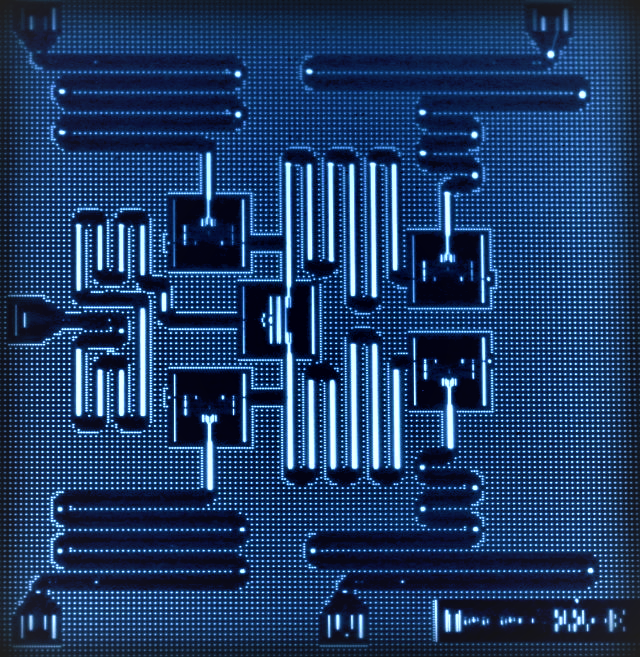
Figure 1.36: IBM QEX2

The IBM Q Experience platform not only allows us to use the composer, but it also allows us to write our code using Open QASM (Quantum Assembly Language). This is a simple text language that has elements of C and assembly languages. By using QASM, we can describe any quantum circuit, in principle, since it has built-in a universal set of quantum gates. In this section, we will discuss how to express quantum circuits and write quantum algorithms using QASM. If we want to discuss the theory behind QASM, we recommend that we read the following paper written by IBM researchers: Open Quantum Assembly Language [233].

Here, we will receive detailed instructions on how to use QASM, we will guide us step by step on how to create our first programs, and we will teach us how to read our results. In this first set of exercises, we will discuss syntax and common mistakes, measurements, single-qubit gates, two-qubit gates, and backends. We will have the opportunity to practice our knowledge and to prove our skills in the end-of-section test. Besides the results that the IBM platform gives us, we will also make a theoretical analysis of the quantum state evolution, so we will easily see the correspondence between the analytical and experimental results.

The numerical simulation employed here is based on the IBM QISKit engine, an open-source package that allows the inclusion of gate and measurement noise, for added realism. This noise model is based on recent calibration data from the 5-qubit IBM QE machines. The output histograms are statistically similar to those that we would obtain from real quantum computers.

By default, each exercise begins with numerical simulations to give us the most rapid feedback for our check-our-understanding answer submission. With select exercises, once our submission is deemed correct, our QASM program will automatically be submitted for execution on a real quantum computer. Once it is run, we should see a plot comparing the simulated and real quantum computer’s results, side-by-side, like this:

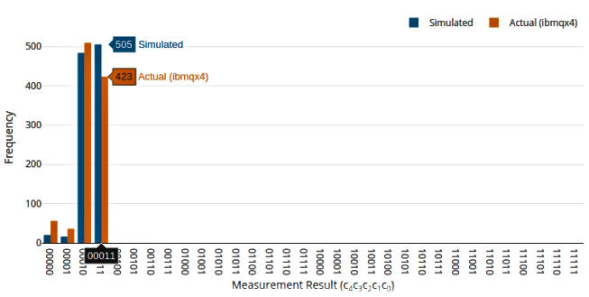
Figure 1.37: Real QC Results Histogram

We will need to be patient, however, because these run requests must be queued for execution since hardware availability is limited. Each program must be run multiple times to generate the output statistics needed for a pedagogical explanation.

1.61   Syntax of QASM

In the figure below, each horizontal line represents the evolution of a qubit with time proceeding from left to right. The five qubits are labeled in order as: q[0], q[1], q[2], q[3] and q[4]. The qubits are always initialized in the quantum state:

$$\lvert 0\rangle=\left(\begin{array}[]{c}1\\ 0\end{array}\right)(1)$$ (1.52)

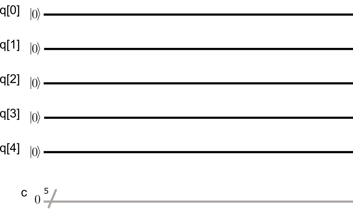
Figure 1.38: Circuit

Classical bits used to store measurement results are indicated by the letter “c” and the number “5” indicates that there are five classical bits in the register being represented with the grey line.

The figure below shows a graphical representation of adding a measurement block to the first qubit. The vertical grey line indicates that the measurement result will be stored in the classical bit register. The number below the grey arrowhead indicates into which classical bit the result will be stored. In this case, the result is stored in bit c[0].

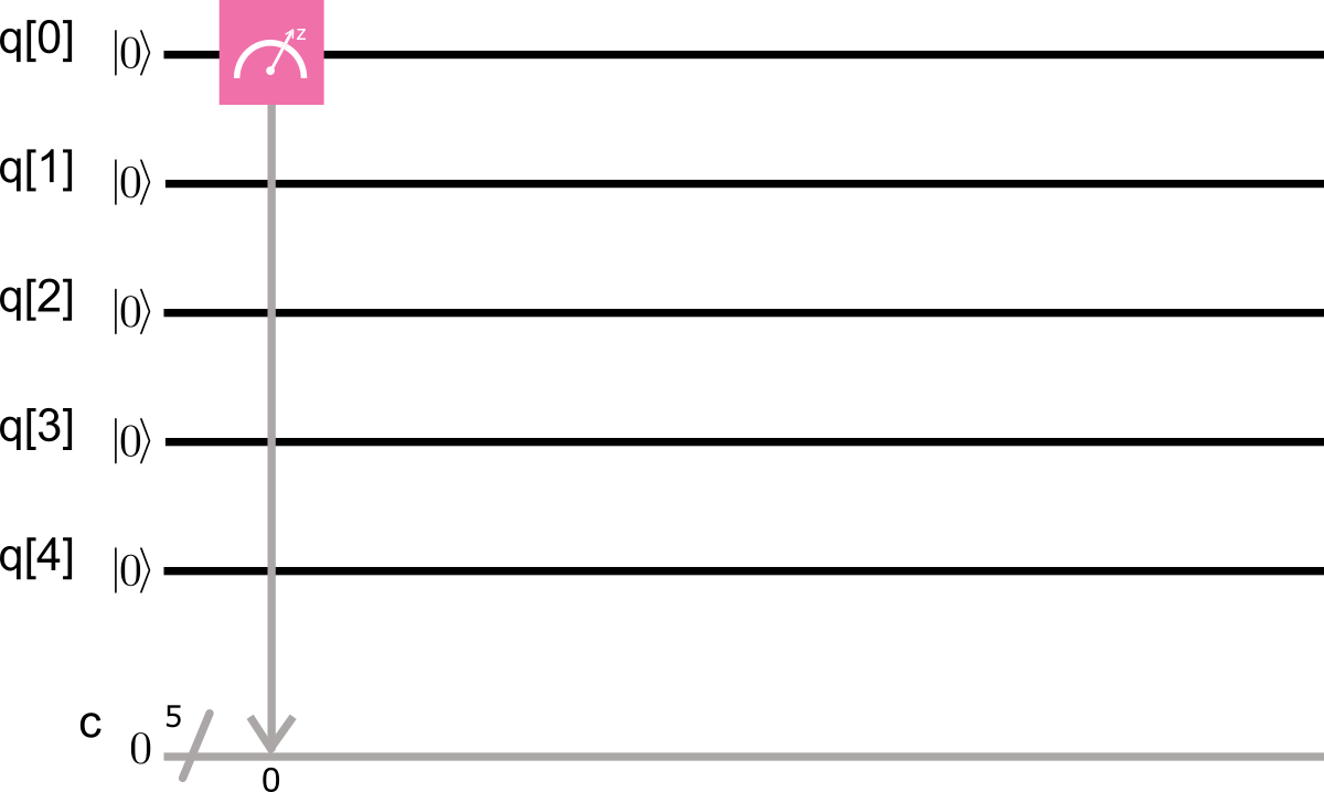
Figure 1.39: Circuit

⬇

1The following QASM code implements the quantum circuit above:

2include ‘‘qelib1.inc’’;

3qreg q[5];

4creg c[5];

5

6// This is a comment

7measure q[0] -> c[0];

Let us take a look at what each line of the previous code does.

Line 1: Includes all gates in the quantum gate library. By adding this, we can then use the X-gate, Y-gate, Z-gate, CNOT gate. Notice that each line has to end in a semicolon “;” (without quotes).

Line 2: Defines a quantum register of five qubits. In this example, we are using five qubits, but we can elect to use any number of qubits from one to five. Note that even if we define a two-qubit register, the quantum circuits depicted here and at the IBM quantum experience site will always graphically illustrate all five qubits by default. This is because the physical quantum computer being used has 5 qubits. Nonetheless, we can choose to work with only a subset of those five qubits.

Line 3: Defines a classical register of five bits. This register is used to store the quantum measurement results. As with the quantum register, even if we define a two-bit classical register, the quantum circuits will indicate all five bits by the grayline. Nonetheless, we can choose to work with only a subset of those five bits.

Line 4: we can insert blank lines to help us organize our sections.

Line 5: we can also insert comments using the “//” (two back-slashes, without quotes). This helps other readers understand our intention in each line. Text that appears after the “//” (without quotes) is not evaluated.

Line 6: Measures the first qubit q[0] and stores the measurement result in bit c[0]. We could alternatively store the information on c[1], but, for organizational purposes, we recommend a direct numerical mapping q[0] to c[0].

1. Syntax Error I, Identify on which line there is an error:
   

   ⬇

   1include‘‘qelib1.inc’’;

   2qreg q[5];

   3creg c[5];

   4measure q[0] -> c[0];

   Solution:
   A space is needed between include and “qelib1.inc”.

2. Syntax Error II, Identify on which line there is an error:
   

   ⬇

   1include ‘‘qelib1.inc’’;

   2qreg q[5];

   3creg c[5]

   4measure q[0] -> c[0];

   Solution:
   There is a missing ; at the end of the line.

3. Syntax Error III, Identify on which line there is an error:
   

   ⬇

   1include ‘‘qelib1.inc’’;

   2qreg q{5};

   3creg c[5];

   4measure q[0] -> c[0];

   Solution:
   Parentesis should be square [] not .

4. Syntax Error IV, Identify on which line there is an error:
   

   ⬇

   1include ‘‘qelib1.inc’’;

   2qreg q[5];\\ this is a comment

   3creg c[5];

   4measure q[0] -> c[0];

   Solution:
   Comments sould be added after // not .

5. Syntax Error V, Identify in which line there is an error:
   

   ⬇

   1include ‘‘qelib1.inc’’;

   2qreg q[2];

   3creg c[2];

   4measure q[0] -> c[2];

   Solution:
   The classical register index should be less than 2. In line 3, creg $c[2]$ defined a classical register with two indexes $c[0]$ and $c[1]$.

   1.62   Measurements

   As we discussed in the previous section, the quantum measurement is probabilistic. When we perform a measurement, we project the state of the qubit onto either $\lvert 0\rangle$ or $\lvert 1\rangle$ with a probability that is the magnitude squared of their respective coefficients (their probability amplitudes). To understand how QASM deals with measurements, Let us go back to the first example,
   

   ⬇

   1include ‘‘qelib1.inc’’;

   2qreg q[5];

   3creg c[5];

   4

   5// This is a comment

   6measure q[0] -> c[0];

   In this example, the first qubit q[0] is measured, and the result of the measurement is stored in classical bit c[0]. The analytical probabilities of projecting q[0] onto states $\lvert 0\rangle$ and $\lvert 1\rangle$ are given by $p(q[0],\lvert 0\rangle)=\lvert\langle 0\lvert 0\rangle\rvert^{2}=1$ and $p(q[0],\lvert 1\rangle)=\lvert\langle 0\lvert 1\rangle\rvert^{2}=0$.

   The IBM QE platform either simulates QASM code or runs it on a real quantum computer, producing numerical results that can be presented as a table. The following figure shows the tabular result of simulating the previous code over 10 “shots” identically prepared and executed experiments. In this example, the qubit was projected 10 times onto state $\lvert 0\rangle$. Note that because the qubit is only projected on to one state in this example, the only label is 0.

   

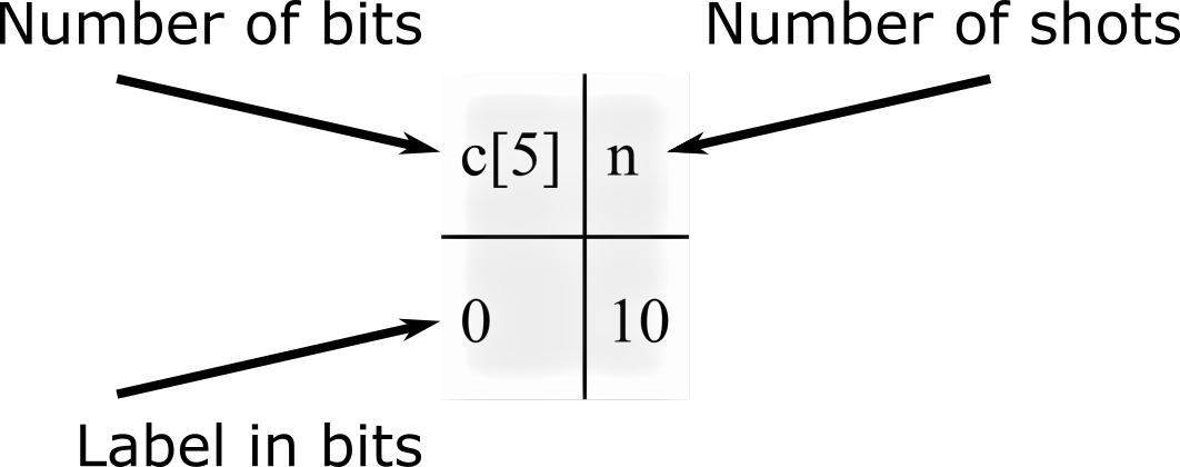
   Figure 1.40: Distribution

   The results are different when the code is run on a real (imperfect) quantum computer. The figure below shows the result of executing the code 8192 times. In this case, there are two different labels because qubit q[0] was projected to state $\lvert 0\rangle$ but was sometimes projected to state $\lvert 1\rangle$. Specifically, it was projected on to $\lvert 0\rangle$ 8182 times and onto $\lvert 1\rangle$ 10 times.

   

   Figure 1.41: Distribution

6. Measuring I, Which option creates a classical register with 3 indexes?
   creg c[0];
   creg c[1]
   creg c[2]
   creg c[3]
   Solution:
   For the classical register to have 3 bits, it must be defined as “creg $c[3]$”, this gives we indices c[0], c[1] and c[2]. The first qubit is labeled q[0], the second is labeled q[1], and so on. To store the second qubit in c[1] we must assign “$q[1]->c[1]$”

7. Measuring II, Which quantum circuit corresponds to the graphical representation of the following code
   

   ⬇

   1include ‘‘qelib1.inc’’;

   2qreg q[5];

   3creg c[5];

   4measure q[1] -> c[3];

   5measure q[3] -> c[1];

   

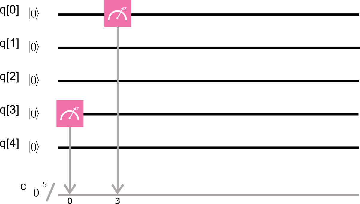
   Figure 1.42: MC 1c

   

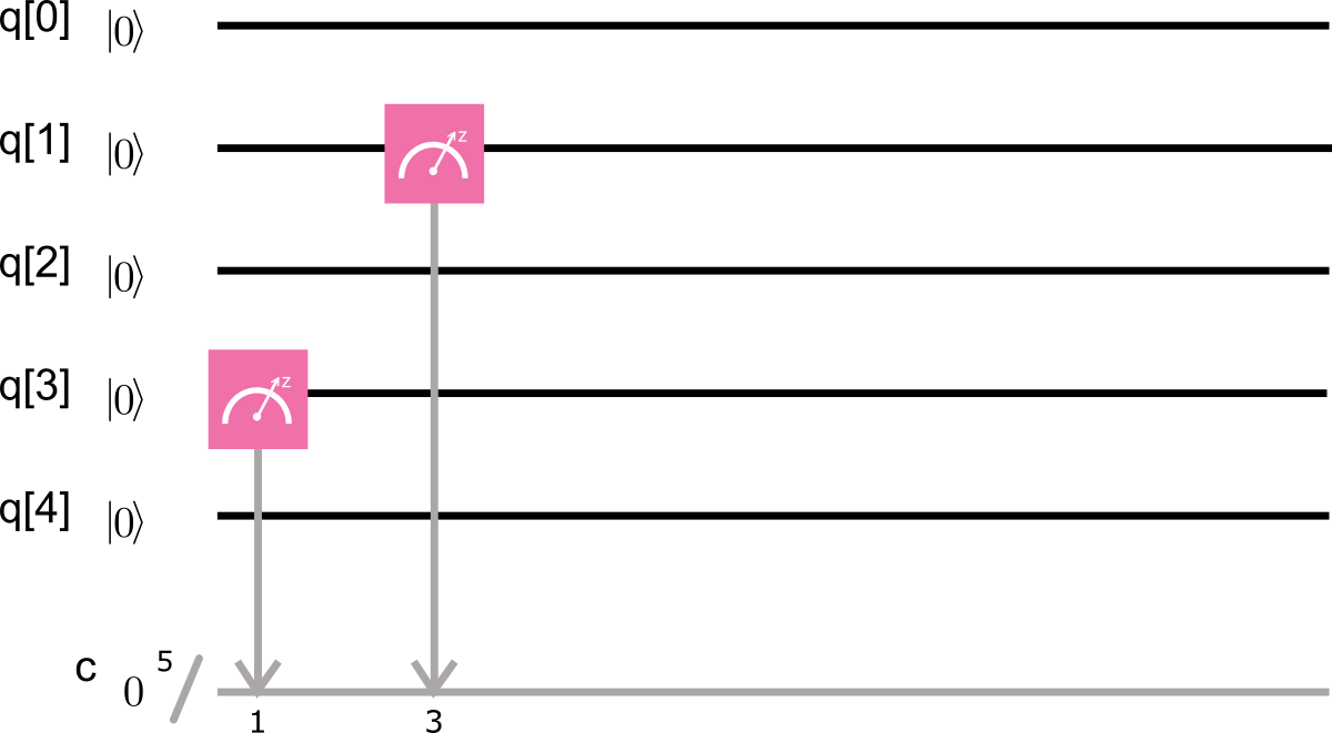
   Figure 1.43: MC 1b

   

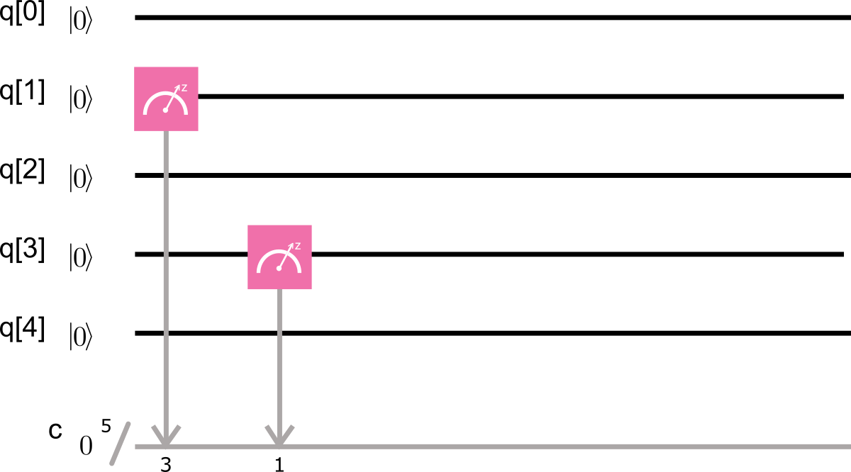
   Figure 1.44: MC 1a

   

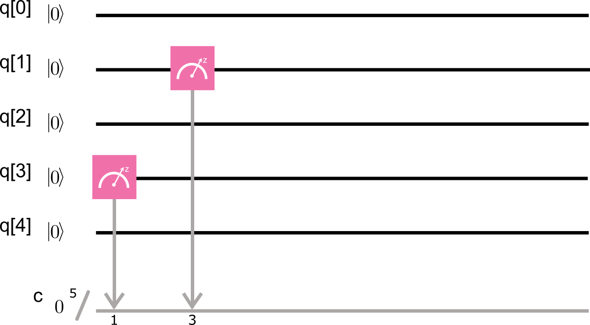
   Figure 1.45: MC 1d

   To better understand how the measurement results are stored in the classical register, Let us consider the quantum circuit below.

   

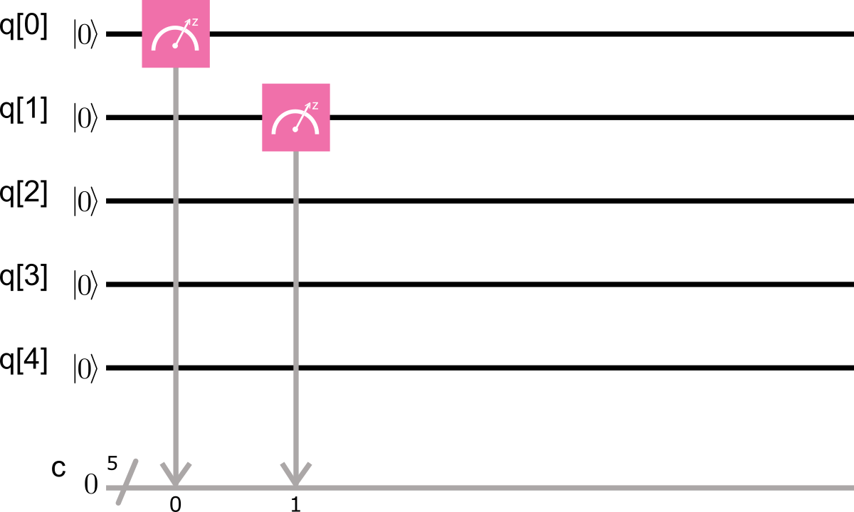
   Figure 1.46: circuit

   The QASM code that generates this circuit is
   

   ⬇

   1include ‘‘qelib1.inc’’;

   2qreg q[5];

   3creg c[5];

   4measure q[0] -> c[0];

   5measure q[1] -> c[1];

   Similar to the previous example, the analytical probabilities of projecting qubits q[0] and q[1] onto states $\lvert 0\rangle$ and $\lvert 1\rangle$ are respectively given by $p(q[0],\lvert 0\rangle)=\lvert\langle 0\lvert 0\rangle\rvert^{2}=1,p(q[0],\lvert 1\rangle)=\lvert\langle 0\lvert 1\rangle\rvert^{2}=0,andp(q[1],\lvert 0\rangle)=\lvert\langle 0\lvert 0\rangle\rvert^{2}=1,p(q[1],\lvert 1\rangle)=\lvert\langle 0\lvert 1\rangle\rvert^{2}=0.$

   The following figure shows the result of simulating the previous code with 10 shots. Qubits q[0] and q[1] were projected 10 times into state $\lvert 0\rangle\lvert 0\rangle$. Note that the label in the left column is “00” because two qubits are being measured.

   

   Figure 1.47: Distribution Updated

   The figure below shows the result of running the previous code in a real quantum computer 1024 times. Since the qubit q[0]measurement was stored in c[0], and q[1] in c[1], the labels are given in the order c[1]c[0]. The number n=1014 at the right of label “00” indicates that qubits q[0] and q[1] were projected onto state $\lvert 00\rangle$ 1014 times. The number n=1 at the right of label “01” indicates that qubits q[0] and q[1] were projected onto state $\lvert 01\rangle$ 1 time. The number n=9 at the right of label “10” indicates that qubits q[0] and q[1] were projected onto state $\lvert 10\rangle$ 9 times. Note that there is no label “11”; this is because the qubits were never projected on to state $\lvert 11\rangle$.

   

   Figure 1.48: Distribution Updated

   The following table shows a summary of the previous results. We can see that the measurement results are in general but not perfect agreement with the analytical probabilities.

   Table 1.2: Results

   Analytical Probabilities	Quantum state $\lvert q[0]q[1]\rangle$	Result Label c[1]c[0]	Projection Frequency n
   1	$\lvert 00\rangle$	00	1014
   0	$\lvert 01\rangle$	10	9
   0	$\lvert 10\rangle$	01	1
   0	$\lvert 11\rangle$	11	0

   To understand how the labeling of the results works can be complicated, so let us analyze the following example.

   

   Figure 1.49: Circuit

   The code that generates this quantum circuit is
   

   ⬇

   1include ‘‘qelib1.inc’’;

   2qreg q[5];

   3creg c[5];

   4measure q[0] -> c[0];

   5measure q[1] -> c[1];

   6measure q[2] -> c[2];

   Since the q[0], q[1] and q[2] measurements are stored in c[0], c[1] and c[2] respectively, the projection results will be stored as in Table 2. If instead the measurements are stored in the following way,
   

   ⬇

   1include ‘‘qelib1.inc’’;

   2qreg q[5];

   3creg c[5];

   4measure q[0] -> c[2];

   5measure q[1] -> c[1];

   6measure q[2] -> c[0];

   then the projection results will be stored as shown in Table 3

   Table 1.3: q[0] $->$ c[0]; q[1] $->$ c[1]; q[2] $->$ c[2]

   Label c[2]c[1]c[0]	Quantum state $\lvert q[0]q[1]q[2]\rangle$
   000	$\lvert 000\rangle$
   001	$\lvert 100\rangle$
   010	$\lvert 010\rangle$
   011	$\lvert 110\rangle$
   100	$\lvert 001\rangle$
   101	$\lvert 101\rangle$
   110	$\lvert 011\rangle$
   111	$\lvert 111\rangle$

   Table 1.4: q[0] $->$ c[2]; q[1] $->$ c[1]; q[2] $->$ c[0]

   Label c[2]c[1]c[0]	Quantum state $\lvert q[0]q[1]q[2]\rangle$
   000	$\lvert 000\rangle$
   100	$\lvert 100\rangle$
   010	$\lvert 010\rangle$
   110	$\lvert 110\rangle$
   001	$\lvert 001\rangle$
   101	$\lvert 101\rangle$
   011	$\lvert 011\rangle$
   111	$\lvert 111\rangle$

   Consider the quantum circuit and measurement results below and respond to the following questions.

   Table 1.5: q[0] $->$ c[2]; q[1] $->$ c[1]; q[2] $->$ c[0]

   c[5]	Quantum state n
   000	7939
   001	113
   010	135
   011	3
   100	11

   

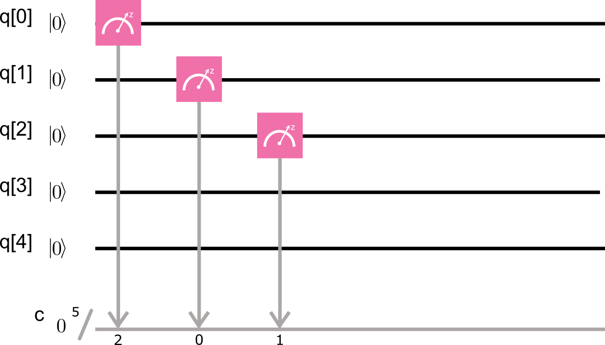
   Figure 1.50: Assessment

8. Measuring III, Which QASM code generates this quantum circuit?
   

   ⬇

   1include ‘‘qelib1.inc’’;

   2qreg q[5];

   3creg c[5];

   4measure q[0] -> c[0];

   5measure q[1] -> c[1];

   6measure q[2] -> c[2];
   ⬇

   1include ‘‘qelib1.inc’’;

   2qreg q[5];

   3creg c[5];

   4measure q[0] -> c[2];

   5measure q[1] -> c[0];

   6measure q[2] -> c[1];
   ⬇

   1include ‘‘qelib1.inc’’;

   2qreg q[5];

   3creg c[5];

   4measure q[0] -> c[2];

   5measure q[1] -> c[1];

   6measure q[2] -> c[0];

9. Measuring IV: How many times was the code run? Solution:
   The sum of all the measurements gives the number of times the experiment is run; 7939+113+135+3+11=8201

10. Measuring V, How many times were the qubits projected to state $\lvert 001\rangle$ Solution:
    The corresponding label to state $\lvert 001\rangle$ is 010. This label shows n=135.

11. Measuring VI, How many times were the qubits projected to state $\lvert 010\rangle$? Solution: The corresponding label to state $\lvert 001\rangle$ is 001. This label shows n=113.

12. Measuring VII, How many times were the qubits projected to state $\lvert 011\rangle$? Solution:
    The corresponding label to state $\lvert 011\rangle$ is 011. This label shows n=3.

13. Measuring VIII, How many times were the qubits projected to state $\lvert 100\rangle$? Solution:
    The corresponding label to state $\lvert 100\rangle$ is 100. This label shows n=11.

    1.63   Single-Qubit Gates

    Up until this point, we have discussed how to measure qubits using QASM and the IBM quantum computer. The IBM platform also enables us to perform single-qubit and two-qubit operations. Table 1 shows the predefined single-qubit gates and the QASM line to apply them on qubit q[0]. We can extrapolate this concept to other qubits.

    Table 1.6: single-qubit gates

    Gate	QASM line
    $X=\left(\begin{array}[]{cc}0&1\\ 1&0\end{array}\right)$	x q[0];
    $Y=\left(\begin{array}[]{cc}0&-i\\ i&0\end{array}\right)$	y q[0];
    $Z=\left(\begin{array}[]{cc}1&0\\ 0&-1\end{array}\right)$	z q[0];
    $H=\frac{1}{\sqrt{2}}\left(\begin{array}[]{cc}1&1\\ 1&-1\end{array}\right)$	h q[0];
    $S=\left(\begin{array}[]{cc}1&0\\ 0&e^{i\frac{\pi}{2}}\end{array}\right)$	s q[0];
    $S^{\dagger}=\left(\begin{array}[]{cc}1&0\\ 0&-e^{i\frac{\pi}{2}}\end{array}\right)$	sdg q[0];
    $T=\left(\begin{array}[]{cc}1&0\\ 0&e^{i\frac{\pi}{4}}\end{array}\right)$	t q[0];
    $T^{\dagger}=\left(\begin{array}[]{cc}1&0\\ 0&-e^{i\frac{\pi}{4}}\end{array}\right)$	tdg q[0];

    In the figure below, an X-gate is applied to the first qubit q[0], and then q[0] and q[1] are measured. The final state of the two-qubit system is given by $\lvert 10\rangle$.

    

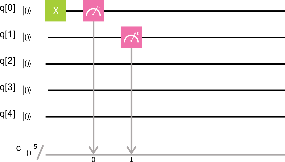
    Figure 1.51: Circuit

    The code below generates the above quantum circuit. Note that there are two blank lines, 4 and 6, this is just to make the code look cleaner. In this way, we will have a first section in which we define our registers, a second section in which we apply the quantum gates, and a third section in which we measure.
    

    ⬇

    1include ‘‘qelib1.inc’’;

    2qreg q[5];

    3creg c[5];

    4

    5x q[0];

    6

    7measure q[0] -> c[0];

    8measure q[1] -> c[1];

    Table 2 shows the results of running the code 1024 times on the perfect quantum simulator. Notice that the two qubits were projected onto state $\lvert 10\rangle$ every time.

    Table 1.7: Results of running the code 1024 times on the perfect quantum simulator

    c[5]	n
    01	1024

    Table 3 shows the results of running the code 1024 times on a real IBM quantum computer. In this case, notice that the two qubits were projected onto state $\lvert 00\rangle$ 70 times, onto state $\lvert 01\rangle 2$ times, onto state $\lvert 10\rangle$ 941 times, and onto state, $\lvert 11\rangle$ 11 times. The difference between the results in tables 2 and 3 are not only given by the errors in the measurements, but also by the error in the X-gate.

    Table 1.8: Results of running the code 1024 times on a real IBM quantum computer

    c[5]	n
    00	70
    01	941
    10	2
    11	11

14. Single-qubit Gates I ) Which code corresponds to the following quantum circuit

    

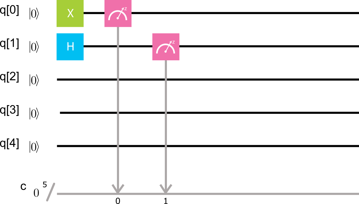
    Figure 1.52: Circuit

    ⬇

    1include ‘‘qelib1.inc’’;

    2

    3qreg q[5];

    4creg c[5];

    5

    6x q[0];

    7h q[1];

    8measure q[0] -> c[0];

    9measure q[1] -> c[1];
    ⬇

    1include ‘‘qelib1.inc’’;

    2

    3qreg q[5];

    4creg c[5];

    5

    6x q[1];

    7h q[2];

    8measure q[1] -> c[1];

    9measure q[2] -> c[2];
    ⬇

    1include ‘‘qelib1.inc’’;

    2

    3qreg q[5];

    4creg c[5];

    5

    6x q[0];

    7h q[1];

    8measure q[0] -> c[1];

    9measure q[1] -> c[0];
    ⬇

    1include ‘‘qelib1.inc’’;

    2

    3qreg q[5];

    4creg c[5];

    5x q[1];

    6h q[2];

    7measure q[1] -> c[2];

    8measure q[2] -> c[1];

    Solution:
    Since an X-gate is applied on qubit q[0], line 6 should be “x q[0]”. Similarly, line 7 should be “h q[1]”, as this is applying a Hadamard gate on qubit q[1].

15. Single-qubit Gates II

    Which the following code generates a quantum circuit

    ⬇

    1include ‘‘qelib1.inc’’;

    2

    3qreg q[5];

    4creg c[5];

    5

    6x q[0];

    7x q[2];

    8measure q[1] -> c[1];

    9measure q[3] -> c[3];

    

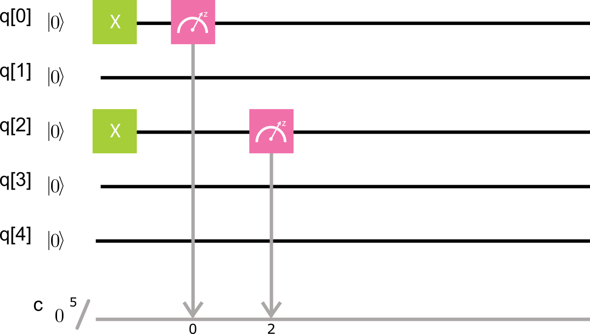
    Figure 1.53: IBM C15a

    

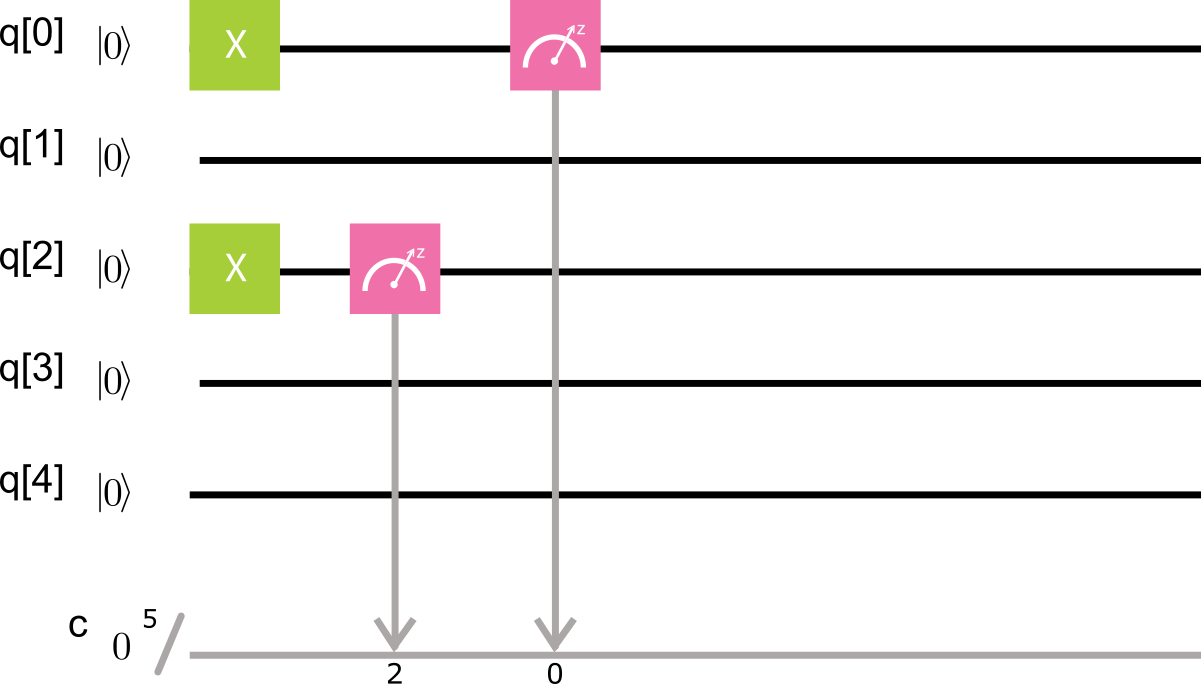
    Figure 1.54: IBM C15b

    

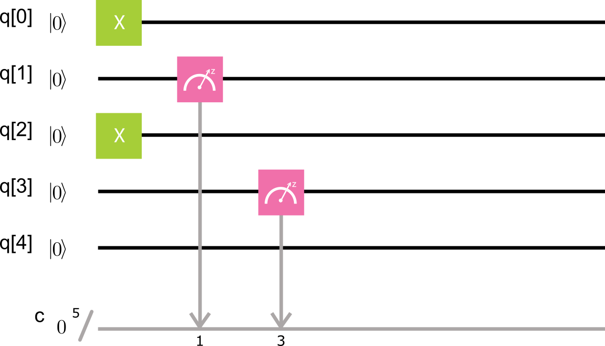
    Figure 1.55: IBM C15c

    

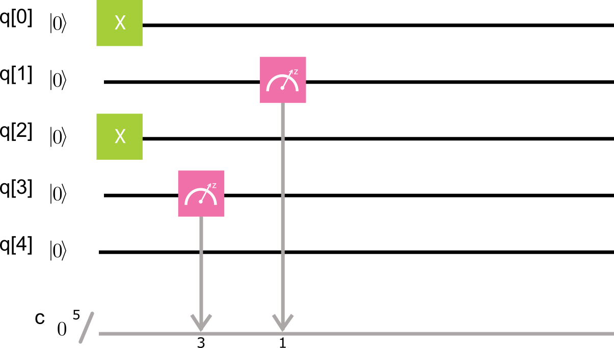
    Figure 1.56: IBM C15d

16. First QASM Code, In the following activity we will run QASM code. Notice that the measurement results will not be given in a tabular format presented as previously, but instead we will see a histogram. Write in the console the following QASM lines:
    

    ⬇

    1include ‘‘qelib1.inc’’;

    2qreg q[5];

    3creg c[5];

    4h q[1];

    5h q[2];

    6measure q[1] -> c[1];

    7measure q[2] -> c[2];

    

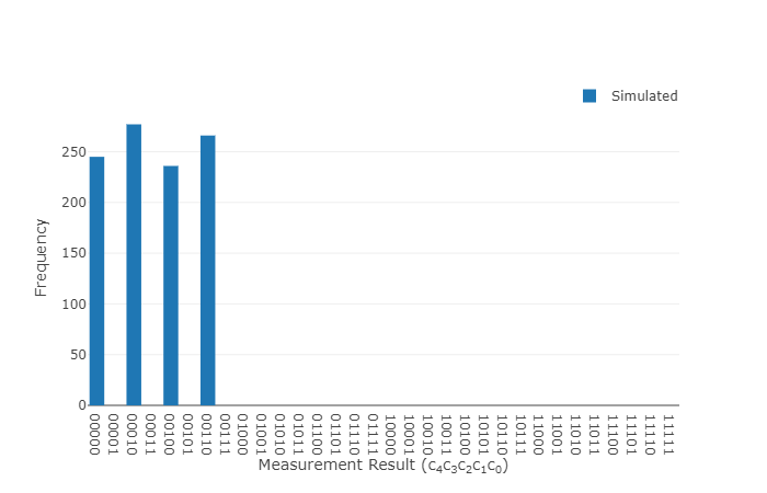
    Figure 1.57: Plot

17. Two Single-Qubit Gates, Write the code that generates the following quantum circuit

    

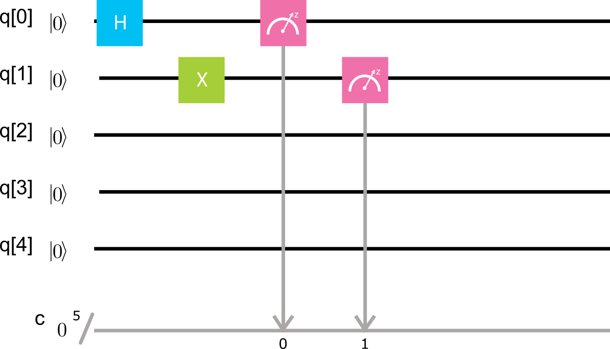
    Figure 1.58: IBM QE2

    ⬇

    1include ‘‘qelib1.inc’’;

    2qreg q[5];

    3creg c[5];

    4h q[0];

    5x q[1];

    6measure q[0] -> c[0];

    7measure q[1] -> c[1];

    Solution:
    Initially, qubits q[0] and q[1] are in the ground state $\lvert 00\rangle$. A Hadamard gate is applied on q[0], and an X-gate on q[1]. This leaves both qubits in the final state $\frac{\lvert 0\rangle+\lvert 1\rangle}{\sqrt{2}}\lvert 0\rangle$. In a perfect simulation, the two-qubit system would project on states $\lvert 01\rangle$ and $\lvert 11\rangle$ with probability 0.5 each.

    

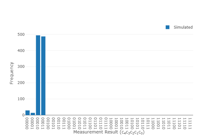
    Figure 1.59: Plot

    1.64   Two-Qubit Gates and Backends

    Controlled NOT Gate

    As we discussed, a universal gate set includes two-qubit gates. A commonly used two-qubit gate is the controlled-NOT operation or CNOT gate. Independent of which qubit is used as the control qubit and which as the target qubit, the CNOT gate will always apply an X-gate onto the target qubit if the control qubit is in the $\lvert 1\rangle$state. When the first qubit is defined as control and the second as a target, the matrix form of the CNOT is given by

    $$CNOT=\left(\begin{array}[]{cccc}1&0&0&0\\ 0&1&0&0\\ 0&0&0&1\\ 0&0&1&0\end{array}\right)$$ (1.53)

    Notice that not all combinations of control and target qubits are allowed in the IBM QE. The combinations that we can use are determined by the topology of the IBM Q experience backend.

    1.64.1 ibmqx2 Backend

    The first backend that we will show is called ibmqx2. The figure below shows its topology.

    

    Figure 1.60: Topology

    The following table shows all the allowed combinations for applying a CNOT-gate in QASM using the ibmqx2 backend.

    Table 1.9: CNOT-gate in QASM

    Control qubit	Target qubit	QASM line
    q[0]	q[1]	cx q[0],q[1]
    q[0]	q[2]	cx q[0],q[2]
    q[1]	q[2]	cx q[1],q[2]
    q[3]	q[2]	cx q[3],q[2]
    q[3]	q[4]	cx q[3],q[4]
    q[4]	q[2]	cx q[4],q[2]

18. CNOT Gate. The following code generates the quantum circuit below.
    

    ⬇

    1include ‘‘qelib1.inc’’;

    2qreg q[5];

    3creg c[5];

    4x q[0];

    5cx q[0],q[1];

    6measure q[0] -> c[0];

    7measure q[1] -> c[1];

    

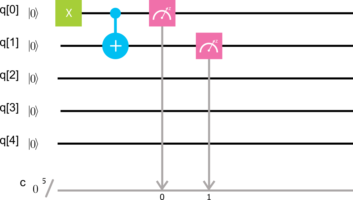
    Figure 1.61: CNIT2

    In the console, write the code that generates the following circuit.

    

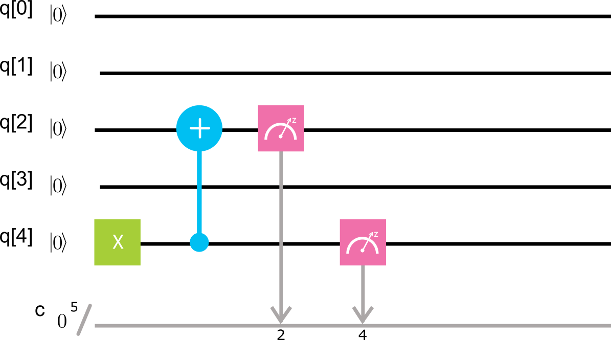
    Figure 1.62: CNOT3

    ⬇

    1include ‘‘qelib1.inc’’;

    2qreg q[5];

    3creg c[5];

    4x q[4];

    5cx q[4],q[2];

    6measure q[2] -> c[2];

    7measure q[4] -> c[4];

    Solution:
    An X-gate is applied on qubit q[4], followed by a CNOT gate with q[4] as control qubit and q[2] as target. The final state of the five qubit system is given by $\lvert 00101\rangle$. The only non-zero analytical probability is $p(q[2]q[4],\lvert 01\rangle)=1$. This is, if the code is run in an perfect quantum computer, the system should always project onto $\lvert 00101\rangle$

    

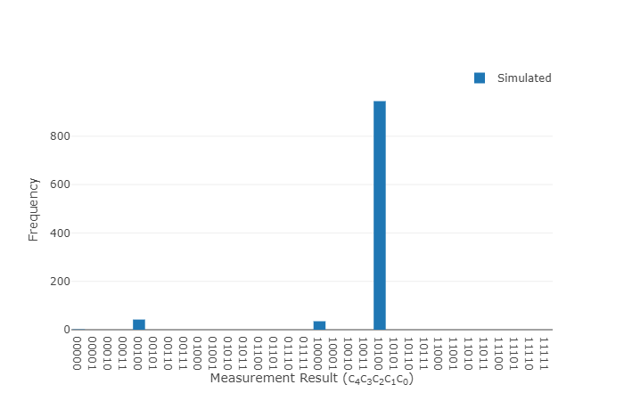
    Figure 1.63: Plot

19. Bell State Creation, In the console, write the code that generates the following circuit

    

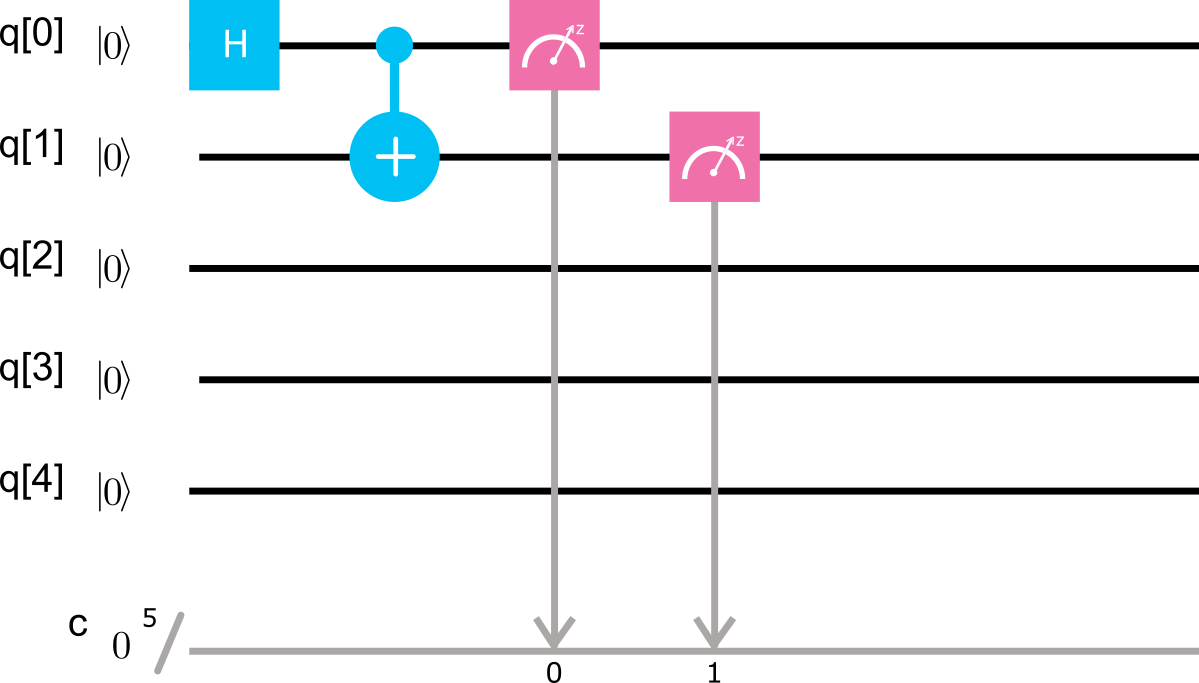
    Figure 1.64: IBM QE4

    ⬇

    1include ‘‘qelib1.inc’’;

    2qreg q[5];

    3creg c[5];

    4h q[0];

    5cx q[0],q[1];

    6measure q[0] -> c[0];

    7measure q[1] -> c[1];

    Solution:
    A Hadamard gate is applied on qubit q[0], followed by a CNOT gate with q[0] as control qubit and q[1] as target. The final state of the five qubit system is given by $\frac{\lvert 00\rangle+\lvert 11\rangle}{\sqrt{2}}$. The non-zero analytical probability are $p(q[0]q[1],\lvert 00\rangle)=0.5$, and $p(q[0]q[1],\lvert 11\rangle)=0.5$.

    

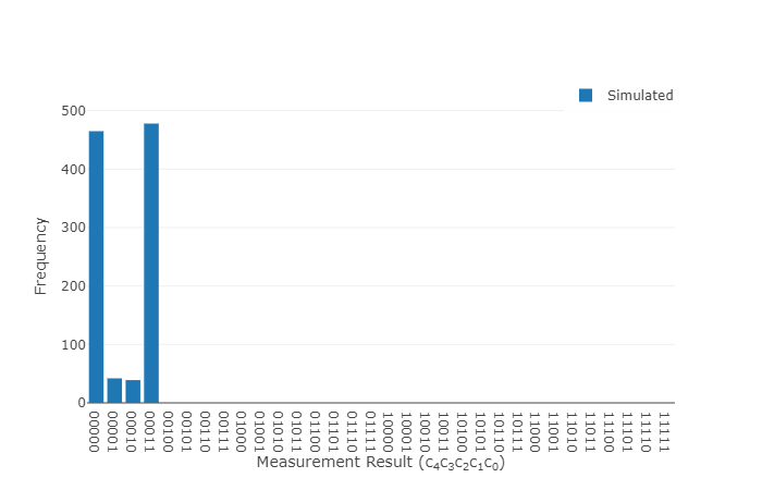
    Figure 1.65: Plot

    1.64.2 ibmqx4 Backend

    The second backend that we will show is called ibmqx4. The figure below shows its topology.

    

    Figure 1.66: Topology 2

    The following table shows all the allowed combinations for applying a CNOT-gate in QASM using the ibmqx4 backend.

    Table 1.10: CNOT-gate in QASM

    Control qubit	Target qubit	QASM line
    q[1]	q[0]	cx q[1],q[0]
    q[2]	q[1]	cx q[2],q[1]
    q[2]	q[0]	cx q[2],q[0]
    q[2]	q[4]	cx q[2],q[4]
    q[3]	q[2]	cx q[3],q[2]
    q[3]	q[4]	cx q[3],q[4]

20. Which of the following QASM programs will work properly with the ibmqx4 backend, meaning that the gates use allowed configurations of control and target qubits? (select all that are valid)
    

    ⬇

    1include ‘‘qelib1.inc’’;

    2

    3qreg q[5];

    4creg c[5];

    5

    6x q[0];

    7h q[1];

    8cx q[0],q[1];

    9

    10measure q[0] -> c[0];

    11measure q[1] -> c[1];

    ⬇

    1include ‘‘qelib1.inc’’;

    2

    3qreg q[5];

    4creg c[5];

    5

    6x q[1];

    7h q[2];

    8cx q[2],q[1];

    9

    10measure q[1] -> c[1];

    11measure q[2] -> c[2];
    ⬇

    1include ‘‘qelib1.inc’’;

    2

    3qreg q[5];

    4creg c[5];

    5

    6x q[2];

    7h q[3];

    8cx q[2],q[3];

    9

    10measure q[2] -> c[2];

    11measure q[3] -> c[3];
    ⬇

    1include ‘‘qelib1.inc’’;

    2

    3qreg q[5];

    4creg c[5];

    5

    6x q[3];

    7h q[4];

    8cx q[3],q[4];

    9

    10measure q[3] -> c[3];

    11measure q[4] -> c[4];

    1.65   N=1 Data Qubit + 1 Ancilla Qubit

    The following quantum circuit is an example of the Deutsch-Jozsa (DJ) algorithm implemented on a single (N=1) data qubit. In this case, the function being evaluated is $f(x)=x_{0}$, and it is balanced. In addition to the data qubit, the DJ algorithm generally needs a second qubit, an ancilla qubit, to facilitate quantum interference during the algorithm evolution.

    In the input register, qubit q[0] serves as the data qubit, and q[1] the ancilla qubit. The Oracle circuit in this case is a CNOT gate, as seen in the composer image:

    

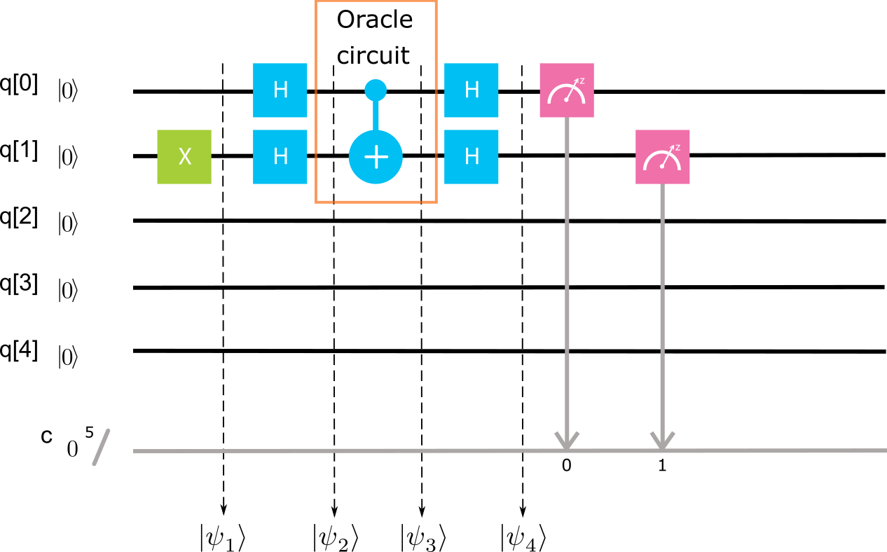
    Figure 1.67: N2 balanced circuit

    Let us now walk through the algorithm step-by-step. All qubits in the IBM Quantum Experience are initialized to state $\left|0\right\rangle$,

    $$\left|\psi_{0}\right\rangle=\left|0\right\rangle\left|0\right\rangle.$$ (1.54)

    Since the ancilla qubit needs to be prepared in state $\left|1\right\rangle$ as prescribed by the DJ algorithm, an X gate is applied to q[1],

    $$\begin{split}\displaystyle\left|\psi_{1}\right\rangle\displaystyle&=\displaystyle\left|0\right\rangle X\left|0\right\rangle,\\ \displaystyle&=\displaystyle\left|0\right\rangle\left|1\right\rangle.\end{split}$$ (1.55)

    Next, a hadamard gate is applied to each qubit to create an equal superposition state of the two qubits.

    $$\begin{split}\displaystyle\left|\psi_{2}\right\rangle\displaystyle&=\displaystyle H\left|0\right\rangle H\left|1\right\rangle,\\ \displaystyle&=\displaystyle\left(\frac{\left|0\right\rangle+\left|1\right\rangle}{\sqrt{2}}\right)\left(\frac{\left|0\right\rangle-\left|1\right\rangle}{\sqrt{2}}\right),\\ \displaystyle&=\displaystyle\frac{1}{2}\left(\left|0\right\rangle\left(\left|0\right\rangle-\left|1\right\rangle\right)+\left|1\right\rangle\left(\left|0\right\rangle-\left|1\right\rangle\right)\right).\end{split}$$ (1.56)

    The Oracle then performs a CNOT gate, with q[0] the control qubit and q[1] the target qubit.

    $$\begin{split}\displaystyle\left|\psi_{3}\right\rangle\displaystyle&=\displaystyle\frac{1}{2}CNOT_{0,1}\left(\left|0\right\rangle\left(\left|0\right\rangle-\left|1\right\rangle\right)+\left|1\right\rangle\left(\left|0\right\rangle-\left|1\right\rangle\right)\right)\\ \displaystyle&=\displaystyle\frac{1}{2}\left(\left|0\right\rangle\left(\left|0\right\rangle-\left|1\right\rangle\right)+\left|1\right\rangle\left(\left|1\right\rangle-\left|0\right\rangle\right)\right)\\ \displaystyle&=\displaystyle\frac{1}{\sqrt{2}}\left(\left|0\right\rangle\left(\frac{\left|0\right\rangle-\left|1\right\rangle}{\sqrt{2}}\right)-\left|1\right\rangle\left(\frac{\left|0\right\rangle-\left|1\right\rangle}{\sqrt{2}}\right)\right)\\ \displaystyle&=\displaystyle\left(\frac{\left|0\right\rangle-\left|1\right\rangle}{\sqrt{2}}\right)\left(\frac{\left|0\right\rangle-\left|1\right\rangle}{\sqrt{2}}\right).\end{split}$$ (1.57)

    Two additional Hadamard gates are then applied to the output state of the oracle, facilitating quantum interference and leading to the output state $\left|f(0)\oplus f(1)\right\rangle$ for q[0] and state $\left|1\right\rangle$ for q[1].

    $$\begin{split}\displaystyle\left|\psi_{4}\right\rangle\displaystyle&=\displaystyle H\frac{\left|0\right\rangle-\left|1\right\rangle}{\sqrt{2}}H\frac{\left|0\right\rangle-\left|1\right\rangle}{\sqrt{2}}\\ \displaystyle&=\displaystyle\left|1\right\rangle\left|1\right\rangle\end{split}$$ (1.58)

    In a DJ algorithm, the function is constant if the values of the data qubits in the output register are all 0’s. Here, they are not, as$f(0)\oplus f(1)=1$, and so the function is confirmed to be balanced.

    Although the DJ algorithm is generally prescribed as N data qubits plus one ancilla qubit, certain specific functions can design a “simplified” or “compiled” version of the oracle that reduces the overhead in implementing the algorithm. In the above graphic, the oracle shown also performs the DJ algorithm on N=2 data qubits for the function $f(x)=x_{0}\oplus x_{1}$. It works, in part, because the function being balanced is determined by $x_{0}$ independent of $x_{1}$ and visa versa. In this “compiled” version of the code, both q[0] and q[1] are data qubits, and q[1] is effectively playing the role of both data qubit and ancilla qubit. At the output, both data qubits are measured and, since they are not both 0’s, the function is confirmed balanced.

21. N=1 Data Qubit, Balanced Function, In the console below write the QASM code that generates the following circuit:

    

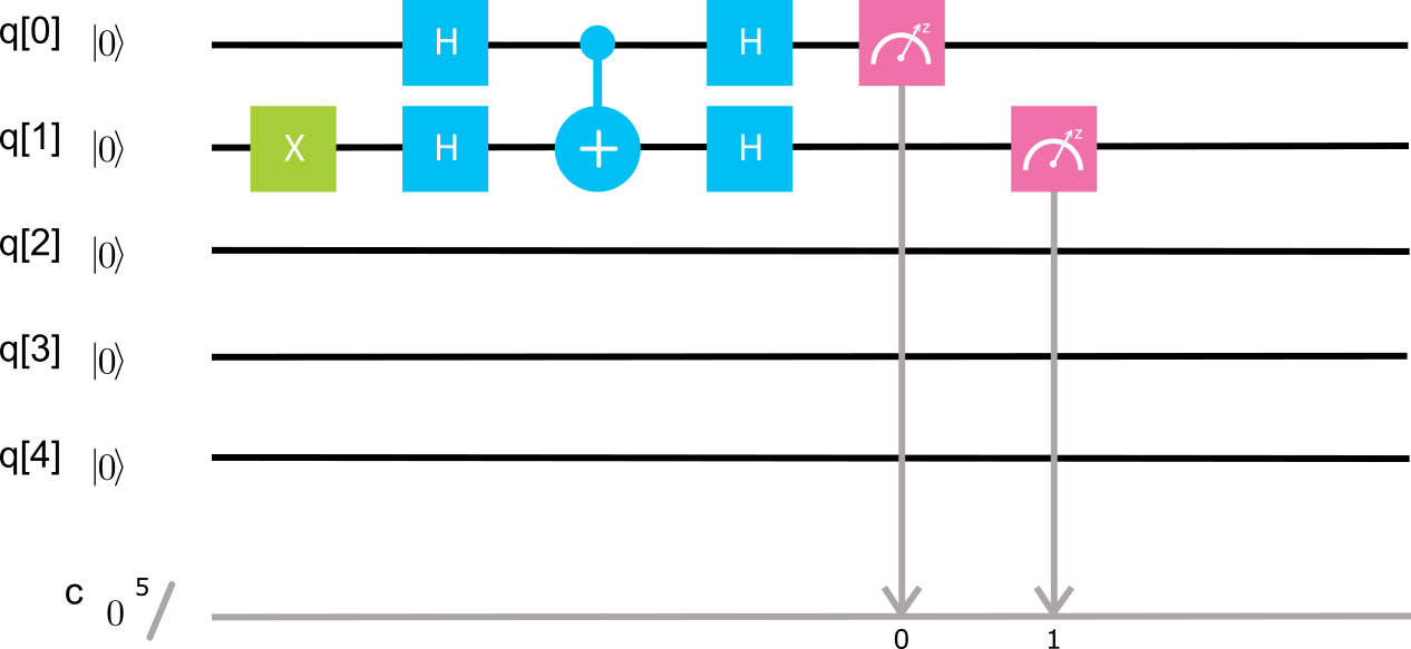
    Figure 1.68: N2 balanced circuit NE

    Submit our response, which will be evaluated with the grader, employing a numerically simulated quantum computer. Once we have a correct submission, our QASM code will automatically be queued to run on a real quantum computer at IBM.
    

    ⬇

    1include ‘‘qelib1.inc’’;

    2qreg q[5];

    3creg c[5];

    4

    5x q[1];

    6h q[0];

    7h q[1];

    8cx q[0],q[1];

    9h q[0];

    10h q[1];

    11measure q[0] -> c[0];

    12measure q[1] -> c[1];

    Solution:
    we just tested the DJ algorithm for N=2 qubits. This circuit implements in above section. Where the top qubit gives $f(0)\oplus f(1)$, and the bottom qubit remains unchanged (so it is 1). Thus, since the function is balanced, $f(0)\oplus f(1)=1$, and we expect the top quit to be 1, and thus both qubits are measured to be 1. The result should thus be a histogram showing $|11\rangle$ with high probability, e.g.:

    

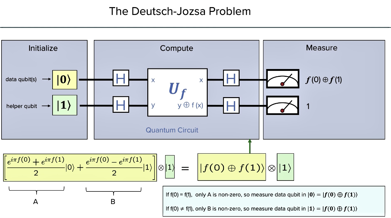
    Figure 1.69: DJ circuit-output

    

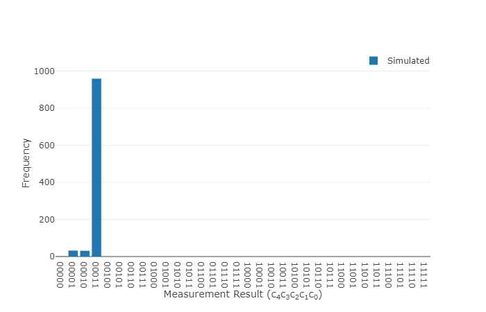
    Figure 1.70: Plot

22. N=1 Data Qubit, Constant Function, In the console below write the QASM code that generates the following circuit:

    

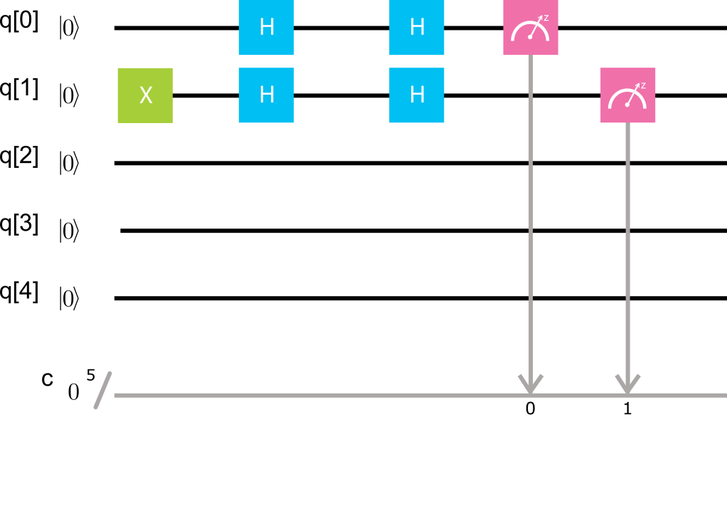
    Figure 1.71: N2 constant circuit

    Submit our response, which will be evaluated with the grader, employing a numerically simulated quantum computer. Once we have a correct submission, our QASM code will automatically be queued to run on a real quantum computer at IBM.
    

    ⬇

    1include ‘‘qelib1.inc’’;

    2qreg q[5];

    3creg c[5];

    4

    5x q[1];

    6h q[0];

    7h q[1];

    8h q[0];

    9h q[1];

    10measure q[0] -> c[0];

    11measure q[1] -> c[1];

    Solution:
    we just tested the DJ algorithm for N=2 qubits for a constant function. Where the top qubit gives $f(0)\oplus f(1)$, and the bottom qubit remains unchanged (so it is 1). Thus, since the function is constant, $f(0)\oplus f(1)=0$, and we expect the top quit to be 0, and thus the output state should be $|01\rangle$. The result should thus be a histogram showing $|11\rangle$ with high probability, e.g.:

    

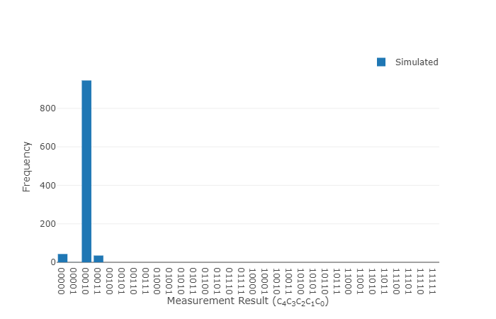
    Figure 1.72: Plot

    1.66   N=3 Data Qubits

    The following quantum circuit is an N=3 data qubit example of the Deustch-Jozsa (DJ) algorithm for a balanced function $f(x)=x_{0}\oplus x_{1}x_{2}$. This function can be understood to be balanced, as toggling the first bit $f(x)=x_{0}$ will toggle the value of f(x) independent of the values of bits $x_{1}$ and $x_{2}$.

    Generally, the DJ algorithm prescribes three data qubits plus one ancilla qubit for this function. However, the oracle circuit shown below is an example of a “compiled” version of the DJ, that is, an implementation that is simplified by design by taking advantage of a particular (but fairly generic) structure of the problem (note the compilation can be done without knowing anything about the answer). In this case, the input register needs only three qubits, all of which are data qubits to test this particular three-bit function f(x). The quantum interference facilitated by the ancilla qubit in the “general” algorithm is built into the oracle circuit in this design.

    

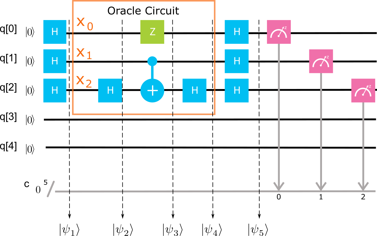
    Figure 1.73: Circuit N3 Balanced

    The three data qubits q[0], q[1], and q[2] are all initialized in state $\left|0\right\rangle$. Note that none of the qubits are initialized in state $\left|1\right\rangle$ as is generally prescribed for the ancilla qubit by the general version of the DJ algorithm.

    $$\left|\psi_{0}\right\rangle=\left|0\right\rangle\left|0\right\rangle\left|0\right\rangle(1)$$ (1.59)

    A three-qubit equal superposition state is then created by applying a Hadamard gate to each qubit.

    $$\begin{split}\displaystyle\left|\psi_{1}\right\rangle\displaystyle&=\displaystyle H\left|0\right\rangle H\left|0\right\rangle H\left|0\right\rangle\\ \displaystyle&=\displaystyle\left(\frac{\left|0\right\rangle+\left|1\right\rangle}{\sqrt{2}}\right)\left(\frac{\left|0\right\rangle+\left|1\right\rangle}{\sqrt{2}}\right)\left(\frac{\left|0\right\rangle+\left|1\right\rangle}{\sqrt{2}}\right)\end{split}$$ (1.60)

    The oracle circuit $U_{f}$ consists a Z-gate on q[0], and a controlled-Z gate (CZ gate), realized by a CNOT gate with q[1] the control qubit and q[2] the target qubit between two Hadamards H applied to q[2]. Starting with the first Hadamard,

    $$\begin{split}\displaystyle\left|\psi_{2}\right\rangle\displaystyle&=\displaystyle\left(\frac{\left|0\right\rangle+\left|1\right\rangle}{\sqrt{2}}\right)\left(\frac{\left|0\right\rangle+\left|1\right\rangle}{\sqrt{2}}\right)\left(H\frac{\left|0\right\rangle+\left|1\right\rangle}{\sqrt{2}}\right)\\ \displaystyle&=\displaystyle\left(\frac{\left|0\right\rangle+\left|1\right\rangle}{\sqrt{2}}\right)\left(\frac{\left|0\right\rangle+\left|1\right\rangle}{\sqrt{2}}\right)\left|0\right\rangle\end{split}$$ (1.61)

    Next, the Z-gate is applied on q[0], and the CNOT gate to q[2] (target) and q[1] (control).

    $$\begin{split}\displaystyle\left|\psi_{3}\right\rangle\displaystyle&=\displaystyle\left(Z\frac{\left|0\right\rangle+\left|1\right\rangle}{\sqrt{2}}\right)CNOT_{1,2}\left(\frac{\left|0\right\rangle+\left|1\right\rangle}{\sqrt{2}}\right)\left|0\right\rangle\\ \displaystyle&=\displaystyle\left(\frac{\left|0\right\rangle-\left|1\right\rangle}{\sqrt{2}}\right)\left(\frac{\left|0\right\rangle\left|0\right\rangle+\left|1\right\rangle\left|1\right\rangle}{\sqrt{2}}\right)\end{split}$$ (1.62)

    And, then the second Hadamard gate is applied to q[2].

    $$\begin{split}\displaystyle\left|\psi_{4}\right\rangle\displaystyle&=\displaystyle\left(\frac{\left|0\right\rangle-\left|1\right\rangle}{\sqrt{2}}\right)\left(\frac{\left|0\right\rangle H\left|0\right\rangle+\left|1\right\rangle H\left|1\right\rangle}{\sqrt{2}}\right)\\ \displaystyle&=\displaystyle\left(\frac{\left|0\right\rangle-\left|1\right\rangle}{\sqrt{2}}\right)\left(\frac{\left|0\right\rangle\left|0\right\rangle+\left|0\right\rangle\left|1\right\rangle+\left|1\right\rangle\left|0\right\rangle-\left|1\right\rangle\left|1\right\rangle}{2}\right)\end{split}$$ (1.63)

    After the oracle circuit, each qubit is again operated on by a Hadamard gate, leaving the final state of the 3 qubits as

    $$\begin{split}\displaystyle\left|\psi_{5}\right\rangle\displaystyle&=\displaystyle H\left(\frac{\left|0\right\rangle-\left|1\right\rangle}{\sqrt{2}}\right)\left(\frac{H\left|0\right\rangle H\left|0\right\rangle+H\left|0\right\rangle H\left|1\right\rangle+H\left|1\right\rangle H\left|0\right\rangle-H\left|1\right\rangle H\left|1\right\rangle}{2}\right)\\ \displaystyle&=\displaystyle\left|1\right\rangle\left(\frac{H\left|0\right\rangle H\left|0\right\rangle+H\left|0\right\rangle H\left|1\right\rangle+H\left|1\right\rangle H\left|0\right\rangle-H\left|1\right\rangle H\left|1\right\rangle}{2}\right)\\ \displaystyle&=\displaystyle\frac{\left|1\right\rangle\left|0\right\rangle\left|0\right\rangle+\left|1\right\rangle\left|1\right\rangle\left|0\right\rangle+\left|1\right\rangle\left|0\right\rangle\left|1\right\rangle-\left|1\right\rangle\left|1\right\rangle\left|1\right\rangle}{2}\end{split}$$ (1.64)

    In each Deutsch-Jozsa algorithm realization, if the data qubits at the output are all 0’s, then the function is constant. Otherwise, it is balanced. In this case, there are no states $\left|0\right\rangle\left|0\right\rangle\left|0\right\rangle$ in the output superposition state with non-zero probability amplitude, and thus any measurement will have at least one of the qubits in-state $\left|1\right\rangle$. Consequently, the function is confirmed to be balanced in just one query.

23. Balanced DJ Algorithm, In the console below write the QASM code that generates the following circuit:

    

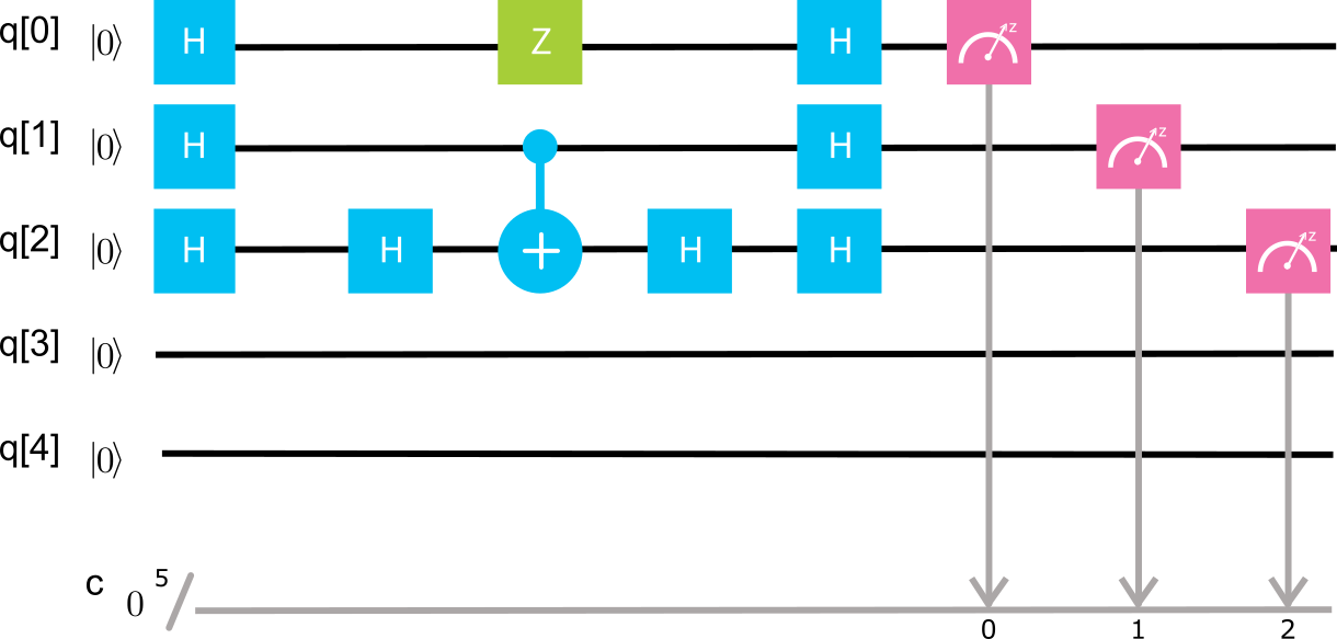
    Figure 1.74: Circuit N3 Balanced NE

    Submit our response, which will be evaluated with the grader, employing a numerically simulated quantum computer. Once we have a correct submission, our QASM code will automatically be queued to run on a real quantum computer at IBM.
    

    ⬇

    1include ‘‘qelib1.inc’’;

    2qreg q[5];

    3creg c[5];

    4

    5h q[0];

    6h q[1];

    7h q[2];

    8h q[2];

    9z q[0];

    10cx q[1],q[2];

    11h q[2];

    12h q[0];

    13h q[1];

    14h q[2];

    15measure q[0] -> c[0];

    16measure q[1] -> c[1];

    17measure q[2] -> c[2];

    Solution: we just tested the DJ algorithm for N=3 qubits. The code was run 1024 times. The expected histogram is something like this: four states with nonzero probability all have the first qubit being equal to 1 this is the signature expected for the function being balanced.

    

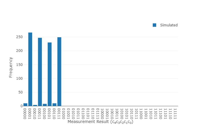
    Figure 1.75: Plot

24. Constant DJ Algorithm, In the console below write the QASM code that generates the following circuit:

    

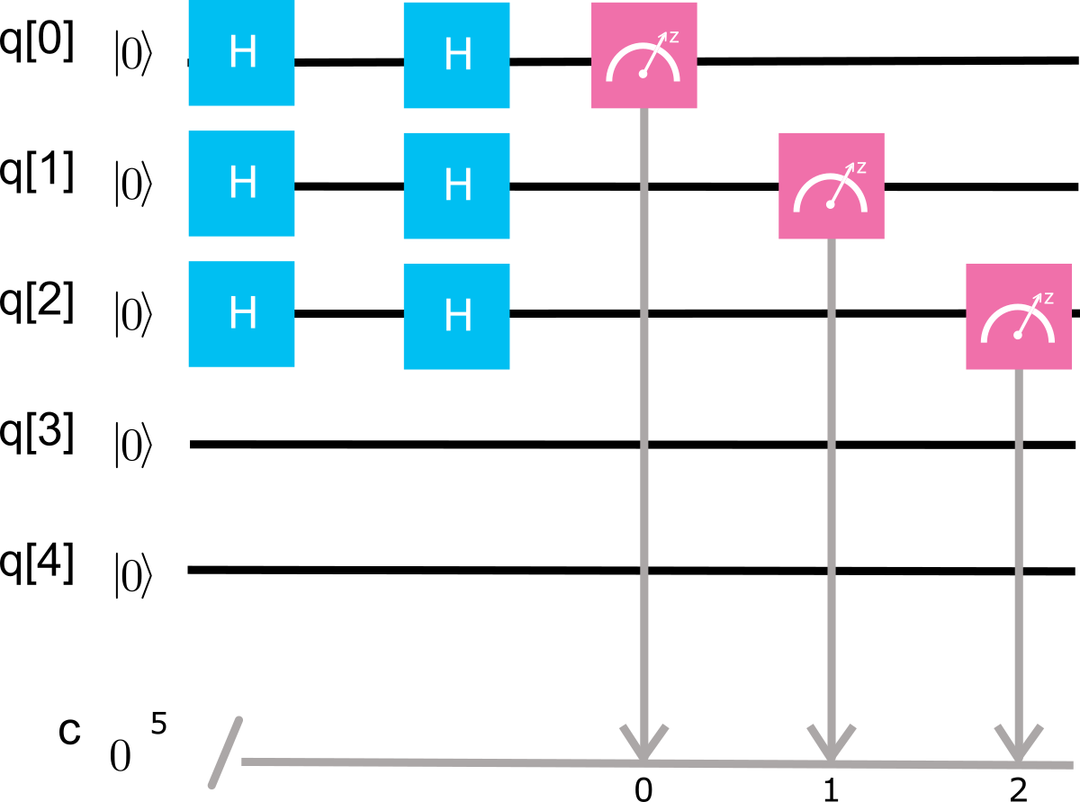
    Figure 1.76: Circuit N3 Constant

    Submit our response, which will be evaluated with the grader, employing a numerically simulated quantum computer. Once we have a correct submission, our QASM code will automatically be queued to run on a real quantum computer at IBM.
    

    ⬇

    1include ‘‘qelib1.inc’’;

    2qreg q[5];

    3creg c[5];

    4

    5h q[0];

    6h q[1];

    7h q[2];

    8h q[0];

    9h q[1];

    10h q[2];

    11measure q[0] -> c[0];

    12measure q[1] -> c[1];

    13measure q[2] -> c[2];

    Solution: we just tested the DJ algorithm for N=3 qubits. The code was run 1024 times. The expected histogram of measurement results is something like this: fact that the output state is all zeros is expected, because all the Hadamard gates pair up and simply cancel each other.

    

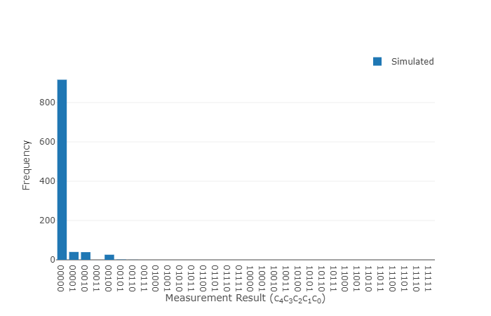
    Figure 1.77: Plot

25. QASM Code I In the console below write the QASM code that generates the following circuit

    

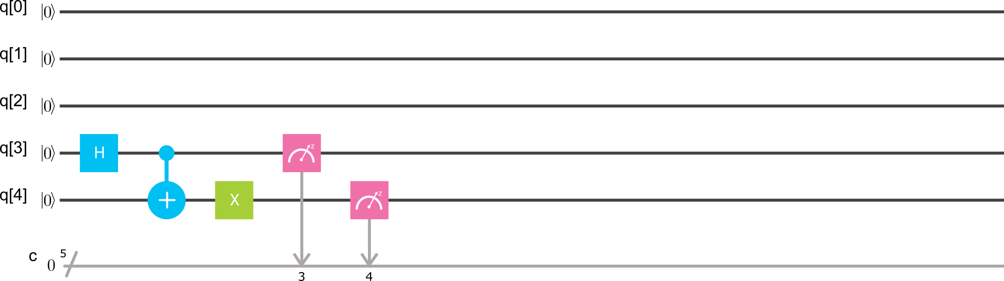
    Figure 1.78: GA1

    ⬇

    1include ‘‘qelib1.inc’’;

    2qreg q[5];

    3creg c[5];

    4

    5h q[3];

    6cx q[3],q[4];

    7x q[4];

    8measure q[3] -> c[3];

    9measure q[4] -> c[4];

    Solution:
    The circuit should act on qubits q[3] and q[4], and produce an output histogram like this one: The output is a superposition of $|00010\rangle and|00001\rangle$; by inspection, this is because the output after the Hadamard and CNOT is (up to normalization) $|00000\rangle+|00011\rangle$; the last X gate then flips the bottom qubit.

    

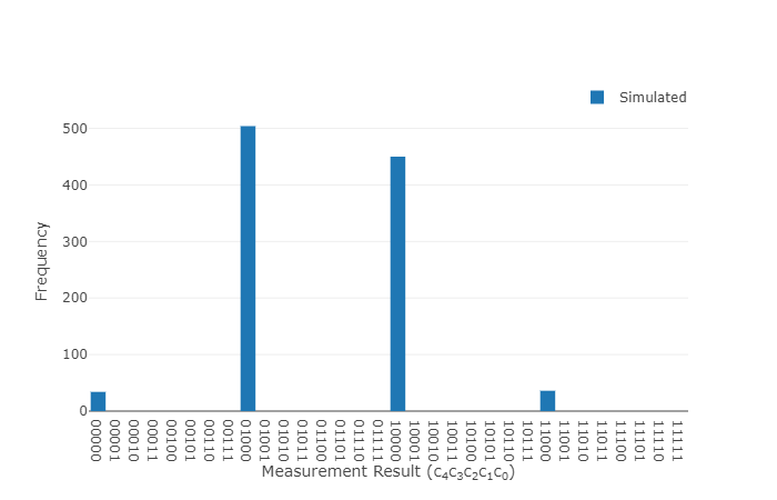
    Figure 1.79: Plot

26. QASM Code II In the console below, write the QASM code that generates the following circuit.

    

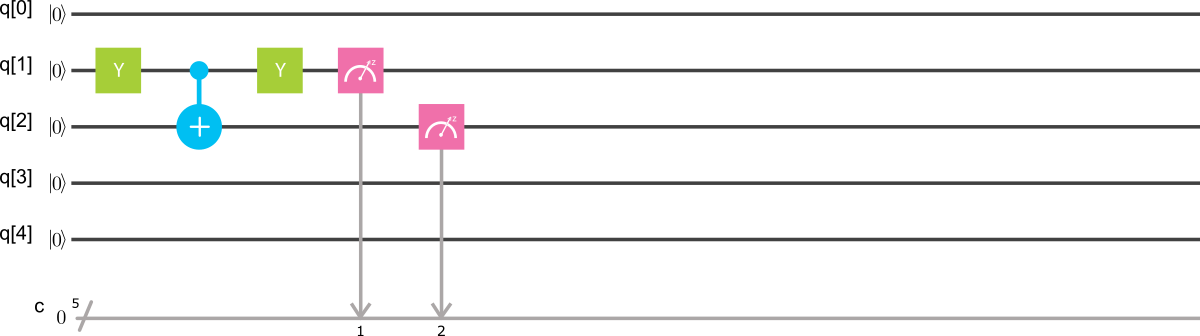
    Figure 1.80: GA2

    ⬇

    1include ‘‘qelib1.inc’’;

    2qreg q[5];

    3creg c[5];

    4

    5y q[1];

    6cx q[1],q[2];

    7y q[1];

    8measure q[1] -> c[1];

    9measure q[2] -> c[2];

    Solution:
    The circuit should act on qubits q[1] and q[2], and produce an output histogram like this one: The output is a single state, $|00100\rangle$; by inspection, this is because the first Y gate flips the control qubit from 0 to 1, causing the CNOT to flip its target qubit; the second Y gate flips the control qubit back to 0.

    

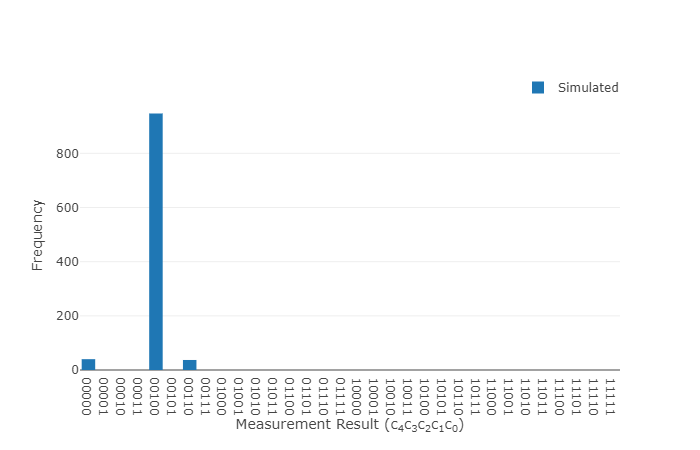
    Figure 1.81: Plot

27. QASM Code III In the console below, write the QASM code that generates the following circuit.

    

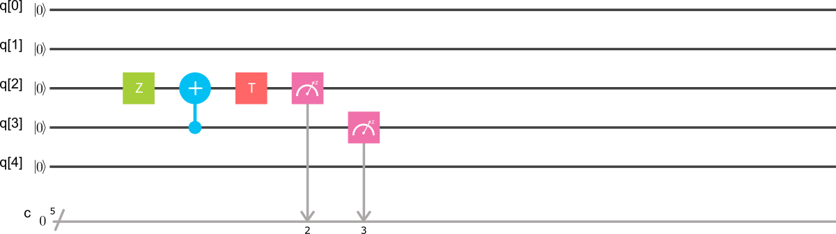
    Figure 1.82: GA3

    ⬇

    1include ‘‘qelib1.inc’’;

    2qreg q[5];

    3creg c[5];

    4

    5z q[2];

    6cx q[3],q[2];

    7t q[2];

    8measure q[2] -> c[2];

    9measure q[3] -> c[3];

    Solution:
    The circuit should act on qubits q[2] and q[3], and produce an output histogram like this one: The output is a single state, $|00000\rangle$; by inspection, this is because the CNOT has a control qubit in the 0 states, so the CNOT does nothing. The Z and T gates also do nothing on their input, the $|0\rangle$ state, so the output is all zeros.

    

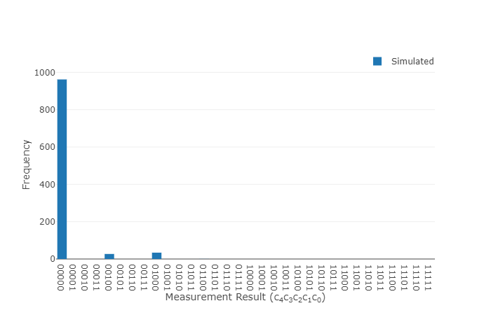
    Figure 1.83: Plot

    

    Figure 1.84: Classical Circuit Model

    

    Figure 1.85: Quantum Circuit Model

    

    Figure 1.86: Quantum Circuit Model

    

    Figure 1.87: The Deutsch-Jozsa Algorithm

    

    Figure 1.88: The Deutsch-Jozsa Algorithm

    

    Figure 1.89: Quantum Software

    

    Figure 1.90: Quantum Software

    

    Figure 1.91: Programming Tools

Index

Part II Quantum-Computation Algorithms

CHAPTER 2  Quantum-Computation Algorithms

Quantum-Computation Algorithms Bhupesh Bishnoibishnoi[At]ieee[Dot]org

In this research notebook on quantum computation and algorithms for quantum engineers, researchers, and scientists, we will discuss and summarized the application of quantum computing algorithms. The most famous quantum algorithm is for factoring numbers. We begin by describing how this algorithm has an enormous potential impact on the world of public-key cryptography. We began by looking at public-key encryption, and Shor’s algorithm, and how Shor’s algorithm can efficiently decrypt, for example, the RSA encryption protocol, which is the basis for information security. We discuss the difference between symmetric and asymmetric keys. We look at classical modern cryptography schemes, which are based on one-way functions. How factoring is performed today and why it is so hard on a classical computer. Furthermore, we went into detail about how Shor’s algorithm can perform this same task, factoring, or order-finding, more efficiently. We first look at it at an intuitive level, and then went through it in mathematically detail. Next, we describe how quantum key distribution provides a method for regaining secure communications, founded upon the basic principles of quantum physics. Thus, we look at how quantum mechanics can break encryption. However, we are also looking at how quantum mechanics can support the encryption of communication protocols, how we can distribute keys using quantum mechanics. We discuss quantum key distribution (QKD) at some level that distributing these symmetric keys using quantum key distribution is an excellent way to encrypt data. So, we want to have a one-time pad at the disposal to encrypt data, but how do we exchange, or continually refresh that one-time pad? Furthermore, that is the task of QKD. We will discuss two general classes of QKD, one based on single-photon sources and detectors, and the other is based on entangled photons and Bell state measurements. Both rely on quantum concepts, which we will be discussing. For example, entanglement, projective measurement, and the no-cloning theorem are essential, so we are expanding on those concepts in detail. We are also going to discuss the importance of randomness in implementing QKD. Pseudo-random number generators that we have on the computers. They are random, but they are generated by the computers using a seed, and so, they are not truly random, never genuinely random. However, the randomness of projective measurements in quantum mechanics allows us to generate what we believe is true randomness. We will discuss how that is used today and the concept of long-distance quantum repeaters. How can we communicate using QKD over long distances when trying to communicate via photons, and photons can be lost or absorbed on an optical fiber? Moreover, in a practical sense, we can probably communicate without quantum repeaters over a metropolitan scale, length scale, but if we start to say, communicate over hundreds of miles or thousands of miles, or beyond, then we need to regenerate this quantum information somehow. The no-cloning theorem puts severe restrictions on what we can do. We cannot simplify amplify the quantum information. We need to develop a quantum repeater, and so, we will discuss that as well. Next, we transition to physicist Richard Feynman’s original application for quantum computer simulation of the quantum systems and how this is now arising as the key near-term application area for the quantum computation field. Finally, we explore another application area in the optimization, by going in-depth into the quantum search algorithm, and implement the algorithm utilizing a real physical quantum computer by IBM Q Experience.

2.1   Introduction to Quantum Information and Cryptography

Quantum computing is investigated worldwide, and we have looked at many efforts that are being done in the United States [242]. Many other efforts are going on worldwide, large efforts in the European Union [243]. They have a flagship program that spends about a billion dollars over the next ten years, investigating quantum computing, quantum communication, and quantum sensing [244]. There are national-level efforts, in Sweden and in Finland, Russia, and Japan [245], Canada [246], Australia [247]. Now many of these are funded by their respective governments, and so different governments have different levels of security. Many of the programs are open, and we can read about them in the public literature, but we should not expect that everything we are seeing is everything that is being done. Many of them are pursuing quantum computing, quantum simulation, universal quantum computation, quantum communication, and quantum sensing. However, in detail, we do not necessarily know what they are doing or what their strategies. In this section, we will manifest quantum mechanical effects that enable quantum computers to process information efficiently [1, 2, 3, 4, 5, 6, 7, 8, 9, 10, 11, 12, 13, 17]. we build on the fundamentals studies to probe more deeply the applications of quantum computing [14, 15] and quantum cryptography [86]. We will not worry about practical issues, like noise at this moment, but rather focused on understanding how these algorithms and protocols work [17]. We will explore the algorithms for cybersecurity, chemistry, and optimization purpose. we want to understand how these algorithms work and their applications. We began by looking at modern cryptography and its use of asymmetric keys, one public, one private, to realize secure public-key cryptography based on one-way functions. We will study in detail one primary example, the RSA cryptosystem [82]. We will discuss that RSA is based on the idea that it is mathematically easy for a classical computer to multiply two large prime numbers, P and Q, and obtain their product N. However. It is a very hard problem for a classical computer to do the inverse, the factor that number N into its constituent primes, P and Q [180]. afterward, we will begin by looking at how Quantum nature can be used to break public-key encryption. We will go into details of Shor’s Algorithm [184], which can efficiently defeat certain important encryption protocols if implemented on a quantum computer. For example, RSA encryption, which serves as the basis for information security today, can be compromised by efficiently performing period finding of modular exponentiation, which is related to prime number factorization. We will look at modern cryptography schemes based on one-way functions. We will look at how factoring is performed and why it is so hard on a classical computer. We will then look at how Shor’s Algorithm can perform the same task in a much more efficient manner, at an intuitive level, and then deep mathematical level into how his algorithm works. Next, we turn to quantum cryptography and discuss how quantum mechanics could enhance communication security through quantum key distribution. We will discuss single-photon generation and detection, and their use in the BB84 QKD protocol. We then look at entangled photons, Bell States, and Bell State measurements [199, noauthor_big_nodate-1], and their uses in the Ekert91 protocol, quantum teleportation, and random number generation.Then, we transition to quantum simulation [33]. We first discuss Hamiltonians, describe the dynamics of a quantum system, and the simulation of those dynamics using Trotterization [81, 211]. We then turn to algorithms, such as phase estimation and variational quantum eigensolvers [56, 100], that address problem in quantum chemistry [218, 91], another hybrid quantum-classical algorithm are variational quantum fidelity estimation algorithm[94], variational quantum factoring (VQF) algorithm [95]. Next, we will discuss adiabatic quantum computing [108, 109], optimization algorithms, the quantum approximate optimization algorithms (QAOA) [21, 248]. We will also discuss quantum annealing [34, 175, 176, 191, 192, 177, 178, 179], and its use of tunneling and relaxation to approach low energy solutions [23]. Although it is not yet known if such processes afford a quantum enhancement, quantum annealers are actively studied in the research, because of optimization problems are ubiquitous. Finally, we will investigate Grover’s Search Algorithm [83], and how it works within the quantum circuit model, and then do prototype experimental demonstrations and implement it on the IBM quantum experience [186].

2.2   Modern Cryptography

We generate and communicate tremendous amounts of digital data every day. Nevertheless, how do we protect this data from eavesdroppers? This section will discuss modern cryptography and how it is used to protect data through encryption. In this section, we will look at modern cryptography schemes and their use in information security today. Every day we generate, accumulate, and communicate tremendous amounts of data. Everything from the personal emails, financial transactions, and medical records, to a corporation’s intellectual property, business strategy, and online sales, to the daily operation and functioning of the government and military organizations. In each of these cases, we expect, even require, that the information is stored and communicated securely such that it is available to ourselves and the intended recipients, but to nobody else. in general, information is protected using encryption. Encryption takes raw data, such as a message, often referred to as plain text, and translates it or encodes it into an unrecognizable message called a cyphertext. It does this by using an algorithm called a cipher. A cipher takes as inputs the plaintext being encoded and a key, typically a numerical bit string in today’s cryptography schemes. The cipher then combines them into an unreadable cyphertext through a prescribed algorithmic protocol based on mathematical operations. Similarly, a decryption key is used with a corresponding decryption protocol to reconstruct the plaintext message. The most common cryptography schemes historically are called symmetric-key cryptography in which the encryption and decryption keys are the same or can be trivially related to one another. Examples include the older data encryption standard, DES, and the more modern advanced encryption standard, AES. The one-time pad that we discussed in section one in the context of quantum key distribution is another example of the symmetric key cryptography scheme. Since symmetric keys are used to both encrypt and decrypt a message, they must remain private. It is not a serious issue, say, a personal computer where we want to encrypt the hard drive, and so, the keys are stored locally. However, it raises a challenge when communicating information. When two parties want to communicate securely, they need to meet in advance to secretly discuss the symmetric keys, not a very practical option, or they need to establish private channels to distribute the key securely. In the future, efficient quantum key distribution protocols may provide a quantum-enhanced security level when transmitting a secret symmetric key. However, today, secure communication links are established using public-key cryptography based on asymmetric keys. Public key cryptography was developed in the 1970s by several groups. Whitfield Diffie and Martin Hellman published the first public-key cryptography scheme, the Diffie-Hellman key exchange protocol, in 1976. Later in 1978, the RSA algorithm was published by Ronald Rivest, Adi Shamir, and Len Adleman. Researchers at the British General Communications Headquarters, GCHQ, had developed similar public-key cryptography schemes in the early 1970s, but only declassified those achievements in 1997. Public key cryptography is based on asymmetric keys. A public key is used for encryption, and a separate independent, private key is used for decryption. The keys are necessarily related to one another mathematically, and the information security relies on it being computationally impractical to determine the private key given the public key. It is possible to use one-way mathematical functions. For example, RSA cryptography [82] is based on the idea that it is mathematically easy for a computer to multiply two large prime numbers, p, and q, and obtain their product, N. However, it is a hard problem for a computer to do the inverse, that is, a factor that number, N, into its constituent prime factors, p, and q[180]. With one-way mathematical functions, ease of use is based on the mathematical simplicity in the forward direction, and security is based on mathematical complexity in the inverse direction. To get an idea for how this works, consider the following cartoon. Bob wants to communicate a message securely to Alice without that message being read by an eavesdropper, Eve. To do this, Bob requests a public encryption key from Alice. Alice then sends a public encryption key but retains her private decryption key. we will represent this by keys with the letter E for encryption, D for decryption, and a notional open lock. During transmission on a public channel, in principle, Eve obtains the open lock and the encryption key. When Bob receives them, he encrypts his plaintext message using the encryption key, creating cyphertext, and effectively locks the padlock. Bob then sends the cyphertext back to Alice on a public channel. Although Eve can obtain the cyphertext in principle, she cannot unlock the padlock since she only has the public encryption key. The security here is based on it is very hard for Eve to figure out the decryption key based on what she has in her possession. Alice, on the other hand, is able to trivially unlock the padlock using her decryption key, thereby converting the cyphertext to plaintext and reading the message. This type of public-key encryption scheme is used ubiquitously today for secure communication. In many cases, it is used to establish a private channel that provides authentication and enables symmetric keys to be exchanged securely. It is because the public key approach based on asymmetric keys is slower to implement than symmetric schemes. Public key encryption is a foundation for information security today. in the next section, we will take a more detailed look at one specific example, RSA cryptography, and how it works.

The Enigma machine is a legendary cipher machine used by German forces before and during World War II. Enigma is an electro-mechanical rotor cipher machine. A message called "plaintext" written by the operator is encoded by the machine similar in appearance to a typewriter in the following manner: a single character is pseudo-randomly replaced with a different letter according to the wiring of the machine. The subsequent letter is replaced following the same mechanism, but with the rotor shifted to a different position. The shifted rotor position causes the letter to be substituted according to a different electrical pathway and hence character substitution table. Thus, each character of the message is replaced according to a different encoding scheme. The resulting "ciphertext" can subsequently be transmitted via regular public communication channels. It can only be decoded using a machine with the same configuration and capability to reverse the encoding. Finally, a successful decipher trial reveals the true content of the message in the form of a plaintext again.

In 1941, at Bletchley Park, a British team, including Alan Turing, uncovered Enigma’s working principles for the Allies. The deciphered information of the intercepted messages provided the Allies with a significant advantage that ultimately became a key element in their victory over the Axis powers.

The Enigma machine is an example of the symmetric encryption scheme, where the same key is used to encode and decode a message. Symmetric encryption schemes are still in use today. However, since World War II, a cryptographic key generation has evolved from electro-mechanical methods to classically constructed digital bit strings serving as encrypting keys. The keys are mathematically challenging to derive and require a significant amount of computational power and time. The computational power and time required to decode are to determine the security of an encoding key.

In 1975, the Data Encryption Standard (DES) was introduced by IBM. The DES algorithm generates a 56-bit symmetric encryption key using a complex mathematical method. Despite this mathematical complexity, DES was known from the beginning to be potentially susceptible to a brute-force key-search attack due to its relatively limited key size. In fact, by the beginning of the 21st century, computational power had sufficiently advanced to the point that one could determine the key in less than a day. For example, Distributed.Net is an organization specializing in the use of idle computer time, utilizing more than 100,000 computers ranging from slow PCs to powerful multiprocessor machines to test 250 billion keys per second and thereby determine a particular 56-bit key in about 23 hours. Given the increasing vulnerability of DES, in 2001, DES was replaced by the Advanced Encryption Standard (AES), a more secure symmetric-key cryptography scheme.

However, there remained a conundrum: how can two parties exchange a symmetric key to initiate secure communication, before they have a secure channel on which to send it? In 1976, a new method for distributing cryptographic keys was introduced by Whitfield Diffie, and Martin Hellman referred to as the Diffie-Hellman key exchange protocol, which heralded the era of public-key cryptography with asymmetric keys. Asymmetric keys comprise a public key used to encrypt messages and a mathematically related (but unique) private key used to decrypt messages. The security of public-key cryptosystems is premised on the use of one-way mathematical functions to create the public and private keys. One-way mathematical functions are straightforward to calculate in the forward direction but prohibitively complex to calculate in the inverse direction. A widely used public-key distribution algorithm was published in 1978 by Ronald Rivest, Adi Shamir, and Len Adleman, referred to as the RSA algorithm. It was later declassified in the late 1990s that asymmetric encryption schemes like RSA were already developed by the British General Communications Headquarters (GCHQ) in the early 1970s. With public-key cryptosystems, one could exchange public keys and establish a secure link, without having symmetric keys in hand at the beginning. Once a secure link was established, one then has the option of continuing to communicate using asymmetric keys, or one can alternatively use this newly established secure link to exchange symmetric keys and use symmetric encryption/decryption protocols.

In practice, public-key encryption techniques are primarily used to establish a secure channel and distribute symmetric keys, which are, in turn, used to encrypt messages. It is because encryption using an asymmetric-key protocol is generally less resource-efficient than using a symmetric-key protocol. For example, a 128-bit symmetric key has $2^{128}$ different possible key combinations. In contrast, a 3000-bit asymmetric key can leverage only the fraction of the $2^{3000}$ possible bit strings that comply with the conditions required by the underlying one-way function. Therefore, whereas the symmetric key of 128 bits and a 3000-bit public key afford a similar level of security, the symmetric-key approach is generally more efficient to implement.

2.3   RSA Cryptosystem

We often communicate securely by encrypting data using cryptographic schemes. However, how do we initiate and establish a secure channel, if we have not yet securely exchanged cryptographic keys? In this section, we will discuss the RSA cryptosystem, a quintessential example of a public-key cryptosystem that leverages asymmetric keys based on one-way mathematical functions to communicate sensitive information.

In the last section, we introduced modern cryptography schemes and discussed the difference between symmetric and asymmetric keys. we discuss that cryptographic algorithms based on symmetric keys have a conundrum when it comes to key distribution. Namely, how can we securely exchange the keys if we do not yet have them in the possession to encrypt the initial transmission? The answer, as we discuss, is to use public-key cryptography based on asymmetric keys. That is, using a public key for encryption and a different private key for decryption. The keys are related to one another mathematically. Their associated information security relies on it being computationally impractical to determine the private key even when we know the public key. This is achieved through the use of one-way mathematical functions where the ease of use of the cryptosystem is based on the mathematical simplicity of implementing the function in the forward direction, and its security is based on the mathematical complexity of implementing it in the reverse or inverse direction. Thus, now, in this section, we will look at a specific quintessential example of public-key cryptography, the RSA cryptosystem, and discuss the fundamentals of how it works. We will discuss communication in the context of Alice and Bob in the presence of an eavesdropper, Eve. Bob would like to send a secure message to Alice. So, he requests her public key, which we will represent here with the letter E. He uses it to encrypt his plain text message, which we will call M, and generate an unreadable cyphertext called C. Alice retains her private key, D, which she uses to decrypt the cyphertext she receives from Bob, and thereby reconstruct the original plain text message. Although Eve has access to the public key and the cyphertext, she cannot decrypt it to reconstruct the plain text message because she does not have access to the private decryption key. because the two keys are mathematically related to one another through a one-way function, computing the private key from what Eve has in hand is, by design, a very hard problem to solve on a classical computer. The RSA cryptosystem is based on a mathematical concept called modular exponentiation. The basic idea is that one can efficiently define three large positive integers, e, d, and N, such that the following expression is true for all integers to m between 0 and N. Namely, m raised to the power e and then raised again to the power d is equal to itself, modulo N. It is very hard for a computer to calculate the number d even when given the numbers e and N. Now this is a fantastic result because it says that Bob can generate cyphertext by taking a plain text message, converting it to an integer N using an agreed-upon protocol, and then raising N to the power e using the public encryption key. Then Alice can decrypt the cyphertext by raising it to the power d to obtain back the number N, modulo N, from which she can reconstruct the plain text message. The public key comprises the numbers e and N, and the private key comprises the numbers d and N. Now, strictly speaking, the only d needs to be kept private, but Alice will need both d and N to do the decryption. With this background, the RSA cryptosystem can be broken into four steps, key generation, key distribution, encryption, and decryption. Let us take them one at a time. Key generation starts with finding two distinct prime numbers, p, and q, a task which can be performed efficiently on a classical computer using mathematical protocols called primality tests. Prime numbers are those that are divisible by only themselves and unity. importantly, these numbers must be chosen at random. we will discuss later in the section more about how quantum mechanics can, in principle, generate true randomness. For now, though, let us assume that we use a pseudo-random number generator on a classical computer. Next, the prime numbers p and q multiply together to generate the number N. Multiplication, which is also efficient on a classical computer. The number N is used as the modulus for both the public and private keys in the performance of modular exponentiation. The next step is to determine the encryption and decryption keys themselves, e and d. This is done using the periodicity property of modular exponentiation. To see this, let us consider a simple example. we will take the number 3 and its exponents, modulo 10. So, 3 to the ith power, modulo 10, where i is an integer, 1, 2, 3. we see that 3 to the first power modulo 10 is 3. 3 squared modulo 10 is 9. 3 cubed is 27, and so, 3 cubed modulo 10 is 7. The modulo 10 is the remainder when dividing 27 by 10. So, 27 divided by 10 is 2 with a remainder 7. Next, 3 to the fourth power is 81, which modulo 10 is 1. continuing, we see that the numbers repeat, 3, 9, 7, 1. 3, 9, 7, 1. Thus, the periodicity here is 4. we will call this periodicity r, So, r equals 4 in this case. Now there is a relationship between the periodicity r and the prime numbers p and q. Consider a general sequence: x modulo N, x squared modulo N, x cubed modulo N, where N equals p times q and x is a number that is not divisible by p or q. Then the sequence has a period r that evenly divides p minus 1-time q minus 1. Let us see how this plays out in the above example. There, the modulus is N equal 10, which has prime factors p equal 2 and q equals 5. 2 times 5 equals 10. Then p minus 1 is 1. q minus 1 is 4. Thus, the quantity p minus 1 time q minus 1 is 1 time 4, and that equals 4. this evenly divides the period r equals 4. So, that checks. What is important here is that this is the one-way function. If we are given prime numbers p and q, then we can calculate the periodicity r. we will not go into how this is done here. we just note that it can be done efficiently on a classical computer, again, if we know the prime numbers p and q. However, if we are just given N, but we do not know p and q, it is hard to find the periodicity r. typically, the periodicity is very large, unlike the simple example given here. So, a brute force search is not efficient either. So, returning to the key generation, Alice has prime numbers p and q. She used them to determine the period r, and she keeps all these numbers private. She now uses r to determine the keys e and d. First, she chooses an integer e in the range 1 to r that is also co-prime with r. That is, e and r have no common divisor other than 1. Now often, this number is simply chosen so that it is not too big and has mostly 0s to enable efficient encryption. For example, 2 to the 16th power plus 1 equal 65,537, which, in binary, is 1 followed by 15 0s and another 1. This is the public encryption key, e. Then the private decryption key is directly calculated from the expression d times e equals 1 modulo r. In summary, Alice generated the public encryption key e and the private decryption key d from the periodicity r based on randomly chosen prime numbers p and q, which multiply together to yield N. Alice keep private the integers p, q, and r, which she used to calculate her private decryption key d. In contrast, the encryption key e and the number N can be made public. In the next step, key distribution, Alice sends Bob the public encryption key e and the number N. Bob has a plain text message that he wants to transmit to Alice securely. He first turns his message into an integer N using an agreed-upon reversible protocol called padding scheme. He then computes the cyphertext c using modular exponentiation and the public key. c equals N to the eth power modulo N. Bob then sends the ciphertext to Alice. Alice then applies her decryption key d to the cyphertext. Using modular exponentiation once more, c to the d-th power, Alice calculates the result, N modulo N. by reversing the padding scheme, Alice recovers the original plain text message. Again, the security of the RSA cryptosystem is based on the use of a one-way function, in this case, the challenge of period finding in modular exponentiation. As we just discussed, if one knows the prime factors p and q, then one can efficiently find the modular exponentiation period r, and thus generate encryption keys e and d. However, if we are just given the modulus N, there is no known efficient classical algorithm that lets us find its prime factors p and q. Thus, there is no efficient means to determine the period r under these conditions. Thus, even if we reveal the modulus N and the public encryption key e, there are no known efficient means for Eve to calculate the private key d, that is, on a classical computer. In the next section, we will look at Shor’s Algorithm and discuss how period finding can be efficiently performed on a quantum computer, thus enabling, in principle, an efficient pathway to breaking the RSA cryptosystem.

Modern cryptography is a foundation for today’s information and economic security, enabling secure communication between individuals, businesses, and governments. There are two basic classes of cryptosystems: symmetric-key and asymmetric-key cryptography. Asymmetric-key cryptography also referred to as public-key cryptography, uses a public key and a private key to encode and decode messages. The two distinct keys are mathematically related via a one-way function, which is computationally efficient to calculate in one direction, but not in the inverse direction.

The workhorse of public-key encryption schemes is the RSA cryptosystem, which can be broken into four steps:

1. key generation (a public key ${\{e,N\}}$and a private key ${\{d,N\}}),$

2. public key distribution,

3. message encryption (a message ${m}\leavevmode\nobreak\$ $\rightarrow$ a ciphertext ${c})$ and transmission,

4. message decryption.

Key Generation and Distribution:

The encryption and decryption keys are generated using a one-way function related to modular exponentiation. To begin with, the two distinct prime numbers p and q are chosen at random. The key generation then centers on the function.

$$f(x)=a^{x}\mod N,$$ (2.1)

Where $a\neq p,q$ is an integer number, the modulus$N=pq$ is the product of p and q, and “mod N" means “modulo N." The term “modular exponentiation" refers to an exponential $a^{x}$ that is calculated modulo N.

From the number theory of modular exponentiation, it is known that the function $f(x)$ is periodic with period r, and finding the value of r is called order finding. Order finding is a manageable task if one knows p and q, but not if one only knows their product N. This is the one-way function under the security of RSA.

To see this, consider the following. When $x=0$ in the above function,

$$f(0)=a^{0}\mod N=1.$$ (2.2)

If f(x) is periodic in r, then it follows that the function f(r), f(2r), f(3r), … must also equal 1. The period r can be derived using Fermat’s little theorem, which uses Euler’s totient function

$$r=(p-1)(q-1)$$ (2.3)

To find the period r.

In essence, Euler’s totient function gives the number of positive integers smaller than the product $pq=N$, which have no prime factors in common with N, that is, co-prime with p, q, and N and Fermat’s little theorem shows that this is the period r. Note that r may be the fundamental period or an integer multiple of the fundamental period. The fundamental period is the least common multiple of $(p-1)$ and $(q-1)$. Both the fundamental period or a multiple of the fundamental period will work.

With p and q are known, the totient can be easily calculated with a classical computer. However, if one is only given N (without knowledge of q and q), then one must factor N to find p and q and thereby find the period r. Factoring is a hard problem for a classical computer[180].

With the period r in hand, one can generate the public key ${\{e,N\}}$ and private key ${\{d,N\}}$. One first chooses a public encryption exponent e that satisfies the following conditions:
1.

$$3\leq e\leq(N-1),$$ (2.4)

2. e is co-prime with r.

The second condition means that there is no integer (other than 1) that divides both e and r, and so their greatest common divisor (gcd) is 1. This is written as $\gcd(e,r)=1.$

Once a value of e is chosen, then one calculates a private decryption exponent d as the modular multiplicative inverse of e, modulo r:

$$d=e^{-1}\mod r$$ (2.5)

Note that when using a modular calculator [249], we will have to use the syntax $A^{B}$mod C and not $\frac{1}{A}$ mod C as the modular multiplicative inverse is only defined for integers. The notation above, while often found, can be misleading in this way.

Intuitively, as we explain in more detail below, the inversion follows that d is used to decrypt a message that is encrypted using e. one can again trivially calculate the private decryption exponent d given the public encryption exponent e, provided one knows the period r.

The steps are summarized in the following table for the specific example of p=17 and q=19.

Table 2.1: p=17 and q=19

1	p,q:	choose two random prime numbers	p= 17, 19
2	N:	calculate N = pq	N = 17*19=323
3	r:	find the period r = ( p-1)(q-1)	r = 16*18=288
4	e:	choose a public exponent e with greatest common divisor gcd (e,r) =1	e =7, gcd(7,288) =1
5	d:	calculate the private exponent $d=e^{-1}\mod r$	d=247

Having created the keys, Alice sends the public key $\{e,N\}$ to Bob. Importantly, she retains the private key $\{d,N\}$, and does not reveal the values p, q, or r.

Message Encryption and Decryption:

Bob has a message m he wants to send to Alice. Having received the public encryption key {e, N}, he encrypts m to create cyphertext c using the public key and modular exponentiation:

$$c=m^{e}\mod N.$$ (2.6)

After the message is sent to Alice, she decrypts it with her private key $\{d,N\}$ using the properties of modular exponentiation,

$$c^{d}\mod N=(m^{e})^{d}\mod N=m$$ (2.7)

provided the original message m is smaller than the modulus N. Eve has access to the public key $\{e,N\}$, but this is no use to her in trying to decrypt the cyphertext, since $c^{e}\mod N\neq m.$

In summary, the number theory and properties of modular exponentiation underlie the security of the RSA cryptosystem. As we have seen, the challenge of order finding can be related to the problem of factoring. While it is straightforward to multiply two numbers p and q to give the modulus N, the inverse problem is hard on a classical computer. If N is chosen sufficiently large, then a brute-force search to find p and q is also inefficient. Thus, the RSA cryptosystem is believed to be securely provided the prime numbers p and q, and the private exponent d are not made public. However, the encryption exponent e and modulus N can be made public. This type of cryptosystem, where the encryption key is public, and anyone can encrypt a message. In contrast, the decryption key is private, and only the receiver can decrypt the cyphertext, which is the backbone of our modern-day communication systems.

2.4   Factoring With a Quantum Computer: Shor’s Algorithm

The security of the RSA cryptosystem is premised on a one-way function that is difficult to invert using a classical computer. However, using Shor’s algorithm, a quantum computer can perform this task much more efficiently. In this section, we will discuss how Shor’s algorithm works.

In the last section, we looked at a specific implementation of public-key cryptography in the RSA cryptosystem. The security of RSA is based on the use of a one-way function prime factorization, which is related to the problem of period finding in modular exponentiation. As we discuss, if one picks two prime numbers, p, and q, which multiply together to give a modulus N, then one can efficiently find the modular exponentiation period r, and thus generate a public encryption key e and a private decryption key d. However, if we are just given the modulus N, then we are stuck, because there is no known efficient classical algorithm that lets us find the prime factors p and q, and so, there is no efficient means to determine the period r. Thus, even if we reveal the modulus N and the public encryption key e, there is no known efficient way for an eavesdropper to calculate the private key d on a classical computer. However, if Eve has access to a quantum computer that can run Shor’s Algorithm, she can efficiently find the modular exponentiation period r. This is called an order finding. Shor’s algorithm finds the order r of a number with respect to the modulus N, where a number is raised to integer powers under modular exponentiation. With a means to efficiently determine, r. Eve can calculate the prime numbers p and q and derive the decryption key d, thus compromising RSA. In this section, we will walk through Shor’s Algorithm using the quantum circuit model presented in section 1 [31]. Then, we will continue with the simple example of modular exponentiation to see the connection between order finding and factorization. Let us begin with the initialization stage. we need two registers of qubits for Shor’s Algorithm. Roughly speaking, Register 1 is used to store the results of a period finding protocol, which is implemented using the Quantum Fourier Transform. we will discuss that one in a moment. Register 2 is used to store the values of the modular exponentiation. This is the function that will apply in the computing section. The number of qubits in the first register should generate a state space that is at least large enough to capture the maximum possible period, and do so, at least twice to see it repeat. Let us define N as twice the maximum period. So, we need at least L qubits, such that 2 to the L power is greater than N. Now, in fact, the more qubits we have, the more densely we can sample the solution space and reduce the error in determining the period. Here, we will take 2L qubits for the first register. for simplicity, we will use the same number of qubits in the second register. By choosing 2L qubits, the number of states 2 to the 2L power is greater than N squared. This guarantees that at least N terms are contributing to the probability amplitude when estimating the period. Even as the period r gets exponentially large, approaching N over 2. we prepare the qubits in state 0, which we denote with a superscripted tensor product, 2L. As we did in section 1 for the Deutsch-Jozsa algorithm, we will track the register states by color yellow for Register 1, and green for Register 2. we will track the current position within the algorithm using the vertical line. Next, at the compute stage, we use Hadamard gates to place the Register 1 qubit into an equal superposition state. Again, we use the superscripted tensor product notation to indicate that we apply a Hadamard gate to each of the 2L qubits. This puts each qubit into a superposition state, 0 plus 1. Multiplying out all 2L of these single qubit superposition states results in a single large equal superposition state with 2 to the 2L components. From a component with 2L qubits in state 0 to a component with all qubits in state 1, and with all combinations in between. If we now number these components from 0 to 2 to the 2L minus 1, we can rewrite the superposition state as a sum over x. Each decimal number x corresponds to one of the binary numbers represented by the 2L qubits. Next, the function f is performed. f of x implements modular exponentiation, which outputs a number a to the x power modulo N. we will not present in detail how the modular exponentiation is implemented in a real circuit. There are multiple approaches to doing it based on reversible computing and multiplication algorithms. For the purposes here, we note that this function can be implemented using ancilla qubits and that it is efficient, requiring several gates that scales only polynomials with the number of qubits[24]. Now, the number is chosen at random, and it must be co-prime with N. That is, it must have no common factors with N. The resulting output values from the function f are then stored in the Register 2 qubits. Since the values of the power x are taken from the qubits in the first register, implementing f of x makes a conditional connection between the qubits in Register 1 and those in Register 2. Although we will not need to measure the qubits in Register 2, this step sets the stage for quantum interference and quantum parallelism to occur in Register 1 at the next step, which is the Quantum Fourier Transform. The Quantum Fourier Transform is a quantum version of the classical discrete-time Fourier Transform. The classical Fourier Transform takes a vector of numbers, x often a digital sampling of a signal to be analyzed and transforms it into a vector of numbers, y, in the frequency domain. Periodic behavior in the time domain is more easily identified in the transformed frequency domain, which is why we do this. For example, a sine wave that oscillates in time with a specific frequency will transform to a large amplitude spike at plus or minus that frequency in the transform domain. Thus, it is easy to identify the spikes’ location and then read off the frequency directly. if we know a signal’s frequency, we also know its period, since the frequency is 1 over the period. Now, the Quantum Fourier Transform is essentially the same transformation, which is why we will use it for period finding. It takes a state j and transforms it into a superposition state with specific phase factors. If we start with a superposition state with coefficients Xj, the transformed result is also a superposition state with coefficients Yk, where the probability amplitudes Yk are the classical discrete-time Fourier Transform of the probability amplitudes Xj. due to quantum parallelism and quantum interference, implementing the Quantum Fourier Transform is exponentially faster than implementing the classical fast Fourier Transform algorithm. Now, that sounds great, but there is an important catch related to quantum measurement. As we know, the measurement of a quantum state is probabilistic. Although the output of the Quantum Fourier Transform is a large superposition state with transformed probability amplitudes, we cannot access those amplitudes. the measurement projects out only a single state, and even if we identically prepare the system and measure it many times, we only discuss the magnitude squared of the corresponding coefficients. we lose the phase information. So, we do not have access to the probability amplitudes in the quantum computer, which is quite different from the classical Fourier Transform, where the entire output vector of complex numbers can be directly read. Thus, the Quantum Fourier Transform is most useful in problems with a unique period or phase that can be found with high probability. For now, let us return to Shor’s Algorithm. The Quantum Fourier Transform is applied here to the qubits in Register 1, and it imparts specific phase factors that are related to both x and z. That is, they are related to both the coefficients of the qubits on Register 1 and the modular exponentiation stored on Register 2. The phase sampling increment is represented here by omega, and it is the phase 2 $\pi$ divided by the total number of states 2 to the 2L power. Here we can see that increasing the number of qubits will reduce the step size, and thus the error in estimating the actual period. Essentially, more qubits will more densely sample the phases that represent the period. Lastly, we measure the qubits in Register 1. The projected state that results is a binary value of z, and its decimal value is equal to or an integer multiple of 2 to the 2L-th power divided by r. Thus, it can be used to find the period r using a continued-fraction expansion of z divided by 2 to the 2L. we can discuss more the Quantum Fourier Transform and related topics in the text units following this section. in the next section, we will take a closer look at how the Quantum Fourier Transform mediates the quantum interference terms that constructively converge to estimates for the period r.

The classical Discrete Time Fourier Transform (DTFT) is a mathematical transformation that takes a vector x of numbers as an input typically a digital sampling of a time-domain signal being analyzed and outputs a vector of numbers y that is its frequency-domain representation:

$$y_{k}=\frac{1}{\sqrt{N}}\sum_{j=0}^{N-1}x_{j}\exp\left(i\frac{2\pi}{N}jk\right)$$ (2.8)

Where N is the total number of points in the vector x, this transform is used ubiquitously in the analysis of signals, because periodic behavior in the time domain is more easily identified in the transformed frequency domain. For example, a sinusoidal signal in time with a frequency f will transform to spikes at $\pm$ f in the frequency domain, find the spikes, and know the frequency of the input signal (or, equivalently, the inverse of its period).

The quantum analog of this transform the Quantum Fourier Transform (QFT) is essentially the same transformation. It takes a single quantum state $\left|j\right\rangle$ and transforms it to a superposition of states, each with specific phase factors:

$$\left|j\right\rangle\rightarrow\frac{1}{\sqrt{N}}\sum_{k=0}^{N-1}\exp\left(i\frac{2\pi}{N}jk\right)\left|k\right\rangle,$$ (2.9)

where N is the total number of states $\left|k\right\rangle$; for n qubits, $N=2^{n}$. If we start with a superposition of states $\left|j\right\rangle$ with coefficients $x_{j}$, then the QFT yields an output superposition of states $\left|k\right\rangle$ with coefficients $y_{k}$,

$$\sum_{k=0}^{N-1}x_{j}\left|j\right\rangle\rightarrow\sum_{k=0}^{N-1}y_{k}\left|k\right\rangle,$$ (2.10)

Where the output amplitudes $y_{k}$ are the DTFT of the input coefficients $x_{j}$. Due to quantum parallelism and quantum interference, the QFT can be implemented using only $(n^{2})$ gates. This is exponentially faster than the Fast Fourier Transform (FFT) algorithm used to calculate the classical DTFT, which requires $O(n2^{n})$ gates.

This sounds terrific, and it is, but there is an important caveat. In general, the QFT cannot be used as a straightforward replacement for the DTFT for real-world data processing applications, and the reason is related to quantum measurement.

In the case of the classical DTFT, even for a real input vector x, the transformed output vector y is complex. We can classically access all of the complex elements of y.

In contrast, in the case of the QFT, a measurement of the output superposition state will project the system into only one of those states with a probability that is the magnitude squared of the corresponding coefficient. We generally have no access to the complex probability amplitudes $y_{k}$. Even if we identically prepare the system and measure it many times, we can only reconstruct the magnitude squared of those coefficients (the magnitude squared of the Fourier spectrum); we have no access to the phase information, and it will take an exponentially large number of measurements to reconstruct the probability for all $2^{n}$ states.

Nonetheless, the QFT is a critical element in quantum computing protocols, including phase estimation and period finding. For these types of applications, the desired output from the QFT is highly localized into a few states with high probability. These states encode the desired information, for example, the period r of modular exponentiation used in Shor’s algorithm.

2.5   Factoring With a Quantum Computer: How Shor’s Algorithm Works

In the last section, we discuss how Shor’s Algorithm is implemented within the circuit model for quantum computing. In this section, we will discuss one more critical step in the algorithm, the application of the quantum Fourier transform.

In the last section, we presented Shor’s Algorithm in the context of the quantum circuit model. we used two registers of qubits. Register 1 was used to store the results of period finding, and Register 2 was used to store the modular exponentiation function’s values. we then applied the Quantum Fourier Transform to Register 1 and measured the output. The projected state resulted in a binary value of z, and its decimal value was an integer multiple of 2 to the 2L divided by r. This, in turn, can be used to find the period r using a continued-fraction expansion. In this section, we will take a closer look at how the Quantum Fourier Transform and the resulting quantum interference lead us to this result. To see how this works, we need to rewrite the sum over x as a combination of two sums. we can use the example of an equal 3 and N equal 10, which we discuss has a period r equal 4. we want to sum over all x from 0 to 2 to the 2L power minus 1. The corresponding function f of x, the modular exponentiation is calculated for several values of x, and the period is, indeed, 4. Let us call the values of x in the first period x0, and the resulting values of the function f we will call w. we see that w has only four unique values and repeats for values of x equal to x0 plus integer multiples of the period r. That is, x0 plus y times r, where we use y as the integer. for a given x0, the function f of x0 plus y r is the same value, as indicated in orange for x0 equals 0. we can see the same behavior for x0 equals 1 in green, x0 equals 2 in blue, and x0 equals 3 in gray. we see that in doing this for the four values of x0, we have covered all values of x. Thus, we can rewrite the sum over x as a sum over the four values of x0 and a sum over the integer y, which runs from 0 to 2 to the Lth power divided by r. Together, these two sums run over all x values from 0 to 2 to the L minus 1. Writing in this way enables us to see how quantum interference occurs with these phase vectors. we first replace omega with its explicit value, e to the power i times 2 $\pi/2$ over 2 to the 2L. there are two-phase factors here. The first is a fixed phase offset independent of the sum over y. It will rotate the phase of any net result that survives the sum. The second is the quantum interference phase related to the sum over y itself. This sum is performed for every value of x0 and z, and it is essentially a test to see if the value of z is related to the period r when starting from a value x0. The sum over y adds together vectors with specific phases related to x0, z, r, and y. In most cases, these phases are not multiples of 2 $\pi$, so the corresponding vectors, according to their phases, end up pointing in various directions, uniformly distributed around the unit circle. Since they point in all directions, adding these vectors gives a net result of 0, which is another example of destructive quantum interference. Now, for a few specific cases where z is related to r through x0, the phases are a multiple of 2 $\pi$. When this is true, the corresponding vectors will always point in the same direction to the right and thus add together constructively. There are 2 to the 2L divided by r unit vectors, and so, the sum is 2 to the 2L divided by r. Mathematically, the sum over y is a geometric sum. we encourage us to calculate this and find the condition which yields non-0 values. we will find the resulting condition is that 2 $\pi/2$ to the 2L times z times r is 2 $\pi$ times an integer, d. Thus, it occurs when z equals d times 2 to the 2 L divided by r. If we plot the probability at the output of the Quantum Fourier Transform, we find a series of spikes that occur when z equals d times 2 to the 2L over r. The probability of measuring any one of these spikes is 1 over r since there are r spikes between 0 and 2 to the 2L over r. This is for a specific value of x0. Whichever one of these spikes we measure, the projected state z with value d times 2 to the 2L over r can be used to find the period r using a continued-fraction expansion procedure. we will not discuss here in detail how that is done. we just note that it is a known algorithm and it can be effectively performed on a classical computer. Now, we just discuss how Shor’s Algorithm can find the period r, but how is this connected to the factoring problem in RSA? Again, we will take the example with N equal 10. we want to find the prime factors p and q that, multiplied together, equal 10. To do this, we randomly pick a number, a that is smaller than N and prime. That is, their Greatest Common Divisor-GCD is unity. we will again choose a equal 3. we then use Shor’s Algorithm to find the period of a to the x modulo N. Shor’s Algorithm, with classical post-processing, will efficiently give us the period r equal 4. Before proceeding, we need to do a couple of checks. First, r must be an even number. second, we need to ensure that a to the r over 2 power plus 1 does not equal 0 modulo N. If we fail either of these tests, we need to go back to step 1 and pick another value of a. However, in the case here, we are fine. For a equal 3 and r equal 4, both conditions check, and we can proceed. we know that a to the r equals 1 modulo N, as this is a property of modular exponentiation. we can rewrite this expression as a to the r-th power minus 1 equals k times N for an integer, k. we then replace N with the unknown prime factors p and q, and we factor the left-hand side to yield a to the r over 2 minus 1 time a to the r over 2 plus 1. Then, p and q can be found from the greatest common divisor of a to the power r over 2 plus or minus 1, and N. Let us take them one at a time. a to the power r over 2 minus 1 is 8. Thus, the greatest common divisor of 8 and 10 is 2, so, p equals 2. Then a to the r over 2 plus 1 is 10, and so, the greatest common divisor of 10 and 10 that is not trivial is 5, so q will equal 5. Therefore, p equals 2, q equals 5, both are prime numbers, and p times q equals 10. Now, this is a very simple example. However, it illustrates how Shor’s Algorithm and period finding can be used to calculate prime numbers p and q, and thus calculate the private decryption key and compromise the RSA cryptosystem. More details and background information related to these topics can be found in the following text units.

2.6   Quantum Fourier Transform

The Quantum Fourier Transform (QFT) is a critical operation used in quantum computing protocols, including period finding and phase estimation. For example, in the period finding protocol, the input state encodes a sequence with an underlying periodic structure, and, following the application of the QFT, the output encodes the period of the sequence.

The QFT is a unitary linear transformation implemented with a series of quantum gates. It maps an n-qubit quantum state $\left|j\right\rangle$ as

$$\left|j\right\rangle\rightarrow\frac{1}{\sqrt{N}}\sum_{k=0}^{N-1}\exp\left(i\frac{2\pi}{N}jk\right)\left|k\right\rangle,$$ (2.11)

N is a constant defined by the number of qubits $N=2^{n}$, and j and k go from 0 to N-1.

Note that the input quantum state can be written as $\left|j\right\rangle$ where j is a decimal number spanning 0 to N-1 (as above), or, equivalently, it can be written as a binary number $\left|j\right\rangle=\left|j_{1}j_{2}...j_{n-1}j_{n}\right\rangle$, where each $j_{i}$ take the value 0 or 1. As short-hand notation, this is sometimes written as the decimal value, e.g. $\left|10\right\rangle=\left|2\right\rangle$ or $\left|11\right\rangle=\left|3\right\rangle.$

In addition to knowing the mapping of the Quantum Fourier Transform, we also need to know how to implement it. For a single-qubit, the mapping of the QFT is:

$$\frac{1}{\sqrt{2^{1}}}\sum_{k=0}^{2^{1}-1}\exp\left(i\frac{2\pi}{2^{1}}0\times k\right)\left|k\right\rangle=\frac{\left|0\right\rangle+\left|1\right\rangle}{\sqrt{2}},$$ (2.12)

$$\frac{1}{\sqrt{2^{1}}}\sum_{k=0}^{2^{1}-1}\exp\left(i\frac{2\pi}{2^{1}}1\times k\right)\left|k\right\rangle=\frac{\left|0\right\rangle-\left|1\right\rangle}{\sqrt{2}},$$ (2.13)

This transformation corresponds to a Hadamard gate,

$$H=\frac{1}{\sqrt{2}}\left(\begin{array}[]{cc}1&1\\ 1&-1\end{array}\right).$$ (2.14)

The figure below shows a graphical representation of the Quantum Fourier Transform for a single-qubit system (the notation $0.j_{1}$ in the exponent is a binary representation that will be introduced below).

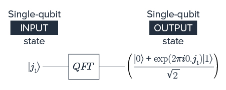
Figure 2.1: Quantum Fourier Transformation

To understand how the Quantum Fourier Transformation works, Let us analyze the two-qubit case, n=2. The state $\left|j\right\rangle$ transforms to:

$$\left|j\right\rangle\displaystyle\rightarrow\displaystyle\frac{1}{\sqrt{2^{2}}}\sum_{k=0}^{2^{2}-1}\exp\left(i\frac{2\pi}{2^{2}}jk\right)\left|k\right\rangle,$$ (2.15)

$$\begin{split}\displaystyle=\displaystyle\frac{1}{\sqrt{2^{2}}}\left(\exp\left(i\frac{2\pi}{2^{2}}j\times 0\right)\left|0\right\rangle+\exp\left(i\frac{2\pi}{2^{2}}j\times 1\right)\left|1\right\rangle\right.\\ \displaystyle\left.+\exp\left(i\frac{2\pi}{2^{2}}j\times 2\right)\left|2\right\rangle+\exp\left(i\frac{2\pi}{2^{2}}j\times 3\right)\left|3\right\rangle\right)\end{split}$$ (2.16)

When the system is initialized in the ground state, j=0, the QFT leaves each qubit in the equal superposition state

$$\frac{\left|0\right\rangle+\left|1\right\rangle}{\sqrt{2}}$$ (2.17)

This is true for any number of qubits n. The QFT maps the ground state of n qubits into n equal superposition single-qubit states,

$$\lvert 00...0\rangle\to\frac{\left|0\right\rangle+\left|1\right\rangle}{\sqrt{2}}\otimes\frac{\left|0\right\rangle+\left|1\right\rangle}{\sqrt{2}}\otimes...\otimes\frac{\left|0\right\rangle+\left|1\right\rangle}{\sqrt{2}}.$$ (2.18)

The table below shows the output state corresponding to each of the values of j.

Table 2.2: output state

$j=0$	$\left|0\right\rangle$	$\frac{1}{\sqrt{2^{2}}}\left(\left|0\right\rangle+\left|1\right\rangle+\left|2\right\rangle+\left|3\right\rangle\right)$
$j=1$	$\left|1\right\rangle$	$\frac{1}{\sqrt{2^{2}}}\left(\left|0\right\rangle+\exp\left(\frac{1}{2}i\pi\right)\left|1\right\rangle+\exp\left(i\pi\right)\left|2\right\rangle+\exp\left(\frac{3}{2}i\pi\right)\left|3\right\rangle\right)$
$j=2$	$\left|2\right\rangle$	$\frac{1}{\sqrt{2^{2}}}\left(\left|0\right\rangle+\exp\left(i\pi\right)\left|1\right\rangle+\left|2\right\rangle+\exp\left(i\pi\right)\left|3\right\rangle\right)$
$j=3$	$\left|3\right\rangle$	$\frac{1}{\sqrt{2^{2}}}\left(\left|0\right\rangle+\exp\left(\frac{3}{2}i\pi\right)\left|1\right\rangle+\exp\left(i\pi\right)\left|2\right\rangle+\exp\left(\frac{9}{2}i\pi\right)\left|3\right\rangle\right)$

When the system consists of more than one qubit and is not initialized in its ground state, the implementation of the QFT is not as simple as implementing Hadamards. To gain insight, Let us write the input and output states as the product of single-qubit states. The input state for an n qubit system is

$$\begin{split}\displaystyle\left|j\right\rangle\displaystyle&=\displaystyle\left|j_{1}j_{2}...j_{n-1}j_{n}\right\rangle,\\ \displaystyle&=\displaystyle\left|j_{1}\right\rangle\otimes\left|j_{2}\right\rangle\otimes...\otimes\left|j_{n-1}\right\rangle\otimes\left|j_{n}\right\rangle\end{split}$$ (2.19)

and the output state is

$$\begin{split}\displaystyle\left|k\right\rangle\displaystyle&=\displaystyle\left|k_{1}k_{2}...k_{n-1}k_{n}\right\rangle,\\ \displaystyle&=\displaystyle\left|k_{1}\right\rangle\otimes\left|k_{2}\right\rangle\otimes...\otimes\left|k_{n-1}\right\rangle\otimes\left|k_{n}\right\rangle\end{split}$$ (2.20)

Next, we should write the indexes j and k in binary using the following procedure:

$$k=k_{1}2^{n-1}+k_{2}2^{n-2}+...+k_{n}2^{0}=\sum_{i=1}^{n}k_{i}2^{n-i},$$ (2.21)

and

$$\frac{j}{2^{n}}=j_{1}2^{-1}+j_{2}2^{-2}+...+j_{n}2^{-n}\equiv 0.j_{1}j_{2}...j_{n}.$$ (2.22)

Note that the notation $0.j_{1}j_{2}...j_{n}$ is new, and the treatment of the entries is position dependent: that is, the position of the variable $j_{n}$ to the right of the “0.” matters, and not it is subscript. For example, the following equivalences follow:

$$0.j_{1}=j_{1}2^{-1}$$ (2.23)

$$0.j_{2}=j_{2}2^{-1}$$ (2.24)

$$0.j_{1}j_{2}=j_{1}2^{-1}+j_{2}2^{-2}$$ (2.25)

$$0.j_{2}j_{4}=j_{2}2^{-1}+j_{4}2^{-2}$$ (2.26)

and so on.

Replacing the terms $k=\sum_{i=1}^{n}k_{i}2^{n-i}$ and $\frac{j}{2^{n}}=0.j_{1}j_{2}...j_{n}$ in equation (1), the n -qubit output state can be written as the product of n single-qubit states

$$\displaystyle\left|j_{1}\right\rangle\otimes\left|j_{2}\right\rangle\otimes...\otimes\left|j_{n-1}\right\rangle\otimes\left|j_{n}\right\rangle$$

$$\displaystyle\rightarrow\displaystyle\left(\frac{\left|0\right\rangle+\exp\left(2\pi i0.j_{n}\right)\left|1\right\rangle}{\sqrt{2}}\right)\otimes\left(\frac{\left|0\right\rangle+\exp\left(2\pi i0.j_{n-1}j_{n}\right)\left|1\right\rangle}{\sqrt{2}}\right)$$

$$\otimes...\otimes\left(\frac{\left|0\right\rangle+\exp\left(2\pi i0.j_{2}...j_{n}\right)\left|1\right\rangle}{\sqrt{2}}\right)\otimes\left(\frac{\left|0\right\rangle+\exp\left(2\pi i0.j_{1}...j_{n}\right)\left|1\right\rangle}{\sqrt{2}}\right).$$ (2.27)

The figure below shows a graphical representation of the Quantum Fourier Transform for an n-qubit system.

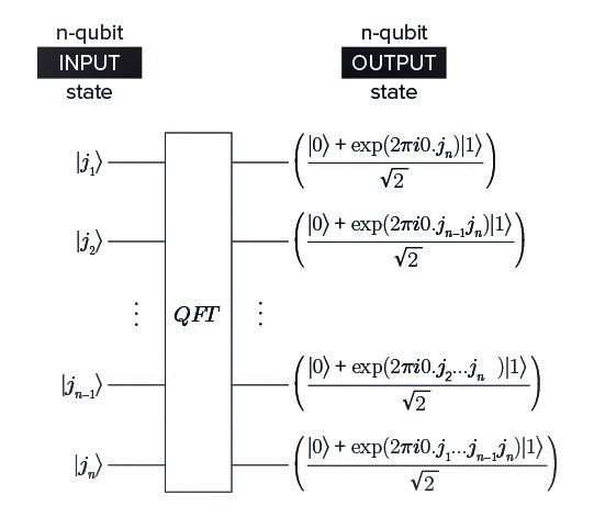
Figure 2.2: Quantum Fourier Transform

To understand how this new representation works, Let us go back to the n=2 example. The table below shows the output state corresponding to each of the values of $j_{1}$ and $j_{2}$. Note, that these states are all written in the single-qubit basis $\left\{\left|00\right\rangle,\left|01\right\rangle,\left|10\right\rangle,\left|11\right\rangle\right\}.$

Table 2.3: output state

	binary to decimal	quantum states
$j_{1}=0,j_{2}=0$	$00\equiv|0\rangle$	$\left|00\right\rangle=\left|0\right\rangle\otimes\left|0\right\rangle$	$\frac{\left|0\right\rangle+\left|1\right\rangle}{\sqrt{2}}\otimes\frac{\left|0\right\rangle+\left|1\right\rangle}{\sqrt{2}}$
$j_{1}=0,j_{2}=1$	$01\equiv|1\rangle$	$\left|01\right\rangle=\left|0\right\rangle\otimes\left|1\right\rangle$	$\left(\frac{\left|0\right\rangle+\exp\left(\pi i\right)\left|1\right\rangle}{\sqrt{2}}\right)\otimes\left(\frac{\left|0\right\rangle+\exp\left(\pi i\frac{1}{2}\right)\left|1\right\rangle}{\sqrt{2}}\right)$
$j_{1}=1,j_{2}=0$	$10\equiv|2\rangle$	$\left|10\right\rangle=\left|1\right\rangle\otimes\left|0\right\rangle$	$\left(\frac{\left|0\right\rangle+\left|1\right\rangle}{\sqrt{2}}\right)\otimes\left(\frac{\left|0\right\rangle+\exp\left(\pi i\right)\left|1\right\rangle}{\sqrt{2}}\right)$
$j_{1}=1,j_{2}=1$	$11\equiv|3\rangle$	$\left|11\right\rangle=\left|1\right\rangle\otimes\left|1\right\rangle$	$\left(\frac{\left|0\right\rangle+\exp\left(\pi i\right)\left|1\right\rangle}{\sqrt{2}}\right)\otimes\left(\frac{\left|0\right\rangle+\exp\left(\pi i\frac{3}{2}\right)\left|\right\rangle}{\sqrt{2}}\right)$

(The binary to decimal column illustrates the connection to the table above, where the decimal short-hand notation was used.)

The single-qubit output states are transformed as:

$$\left|0\right\rangle\displaystyle\rightarrow\displaystyle\frac{\left|0\right\rangle+\left|1\right\rangle}{\sqrt{2}},$$ (2.28)

$$\left|1\right\rangle\displaystyle\rightarrow\displaystyle\frac{\left|0\right\rangle+\exp\left(i\phi_{m}\right)\left|1\right\rangle}{\sqrt{2}}$$ (2.29)

where $\phi_{m}$ is a phase between 0 and $2\pi$. If the input state is $\left|0\right\rangle,$ then the output state is always an equal superposition state with zero relative phase. If the input state is $\left|1\right\rangle,$ then the output is an equal superposition state, but with a phase shift $\exp\left(i\phi_{m}\right)$ on state $\left|1\right\rangle.$ Specifically, for n qubits, the phase of the first output qubit is $\phi_{1}=2\pi 0.j_{n},$ the second is $\phi_{2}=2\pi 0.j_{n-1}j_{n},$ the third is $\phi_{3}=2\pi 0.j_{n-2}j_{n-1}j_{n},$ and so on until the last qubit which phase is $\phi_{n}=2\pi 0.j_{1}...j_{n}.$

There are two takeaways:
1. When the input state is $\left|0\right\rangle,$ the output state is an equal superposition state with zero relative phases.
2. When the input state is$\left|1\right\rangle,$ the output state is an equal superposition state that undergoes a relative phase rotation.

From these two points, it is clear that the implementation of the QFT is related to a controlled operation that modifies a qubit state, as shown in the table below.

From these two points, it is clear that the implementation of the QFT is related to a controlled operation that modifies a qubit state as shown in the table below.

Table 2.4: QFT

Controlled Operation
Input state	Output state
$\left|0\right\rangle$	$\frac{\left|0\right\rangle+\left|1\right\rangle}{\sqrt{2}}$
$\left|1\right\rangle$	$\frac{\left|0\right\rangle+R_{k}\left|1\right\rangle}{\sqrt{2}}$

The figure below shows the circuit implementation of the Quantum Fourier Transform in terms of multiple Hadamard gates and controlled $R_{k}$ gates. The phase rotation $R_{k}$ is defined as

$$R_{k}\left|0\right\rangle\displaystyle=\displaystyle\left|0\right\rangle,$$ (2.30)

$$R_{k}\left|1\right\rangle\displaystyle=\displaystyle\exp\left(i\frac{2\pi}{2^{k}}\right)\left|1\right\rangle.$$ (2.31)

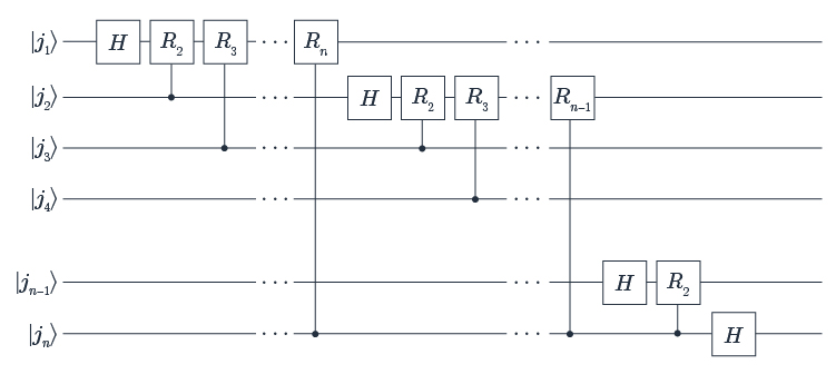
Figure 2.3: Quantum Fourier Transform

Let us analyze how the system evolves under this implementation.

1. A Hadamard gate is applied on the first qubit

$$\lvert j_{1}\rangle\rightarrow\frac{\lvert 0\rangle+\exp(2\pi i0.j_{1})\lvert 1\rangle}{\sqrt{2}},$$ (2.32)

and this puts the system in the state

$$\frac{\left|0\right\rangle+\exp\left(2\pi i0.j_{1}\right)\left|1\right\rangle}{\sqrt{2}}\otimes\left|j_{2}\right\rangle\otimes\left|j_{3}\right\rangle\otimes...\otimes\left|j_{n}\right\rangle.$$ (2.33)

2. A controlled phase $R_{2}$-gate is applied with the second qubit as control and the first as target,

$$\frac{\left|0\right\rangle+\exp\left(2\pi i0.j_{1}j_{2}\right)\left\lvert 1\right\rangle}{\sqrt{2}}\otimes\left\lvert j_{2}\right\rangle\otimes\left\lvert j_{3}\right\rangle\otimes...\otimes\left|j_{n}\right\rangle.$$ (2.34)

3. A controlled phase $R_{3}$-gate is applied with the third qubit as control and the first as target,

$$\frac{\left|0\right\rangle+\exp\left(2\pi i0.j_{1}j_{2}j_{3}\right)\left|1\right\rangle}{\sqrt{2}}\otimes\left|j_{2}\right\rangle\otimes\left|j_{3}\right\rangle\otimes...\otimes\left|j_{n}\right\rangle.$$ (2.35)

4. This continues until a controlled phase $R_{n}$-the gate is applied with the last qubit as control and the first as a target, leaving the system in the state

$$\frac{\left|0\right\rangle+\exp\left(2\pi i0.j_{1}j_{2}j_{3}...j_{n}\right)\left|1\right\rangle}{\sqrt{2}}\otimes\left|j_{2}\right\rangle\otimes\left|j_{3}\right\rangle\otimes...\otimes\left|j_{n}\right\rangle.$$ (2.36)

5. A Hadamard gate is applied on the second qubit,

$$\left(\frac{\left|0\right\rangle+\exp\left(2\pi i0.j_{1}j_{2}j_{3}...j_{n}\right)\left|1\right\rangle}{\sqrt{2}}\right)\otimes\left(\frac{\left|0\right\rangle+\exp\left(2\pi i0.j_{2}\right)\left|1\right\rangle}{\sqrt{2}}\right)\otimes\left|j_{3}\right\rangle\otimes...\otimes\left|j_{n}\right\rangle.$$ (2.37)

6. A controlled phase $R_{2}$-gate is applied with the third qubit as control and the second as target,

$$\left(\frac{\left|0\right\rangle+\exp\left(2\pi i0.j_{1}j_{2}j_{3}...j_{n}\right)\left|1\right\rangle}{\sqrt{2}}\right)\otimes\left(\frac{\left|0\right\rangle+\exp\left(2\pi i0.j_{2}j_{3}\right)\left|1\right\rangle}{\sqrt{2}}\right)\otimes\left|j_{3}\right\rangle\otimes...\otimes\left|j_{n}\right\rangle.$$ (2.38)

7. This continues until a controlled phase $R_{n-1}$-gate is applied with the last qubit as control and the second as target, leaving the system in the state

$$\frac{\left|0\right\rangle+\exp\left(2\pi i0.j_{1}j_{2}j_{3}...j_{n}\right)\left|1\right\rangle}{\sqrt{2}}\otimes\frac{\left|0\right\rangle+\exp\left(2\pi i0.j_{2}j_{3}...j_{n}\right)\left|1\right\rangle}{\sqrt{2}}\otimes\left|j_{3}\right\rangle\otimes...\otimes\left|j_{n}\right\rangle.$$ (2.39)

8. This same process is done on each qubit until the last qubit, on which we can only apply a Hadamard gate. This implementation transforms as

$$\displaystyle\left|j_{1}\right\rangle\otimes\left|j_{2}\right\rangle\otimes...\otimes\left|j_{n-1}\right\rangle\otimes\left|j_{n}\right\rangle$$

$$\displaystyle\rightarrow\displaystyle\left(\frac{\left|0\right\rangle+\exp\left(2\pi i0.j_{1}...j_{n}\right)\left|1\right\rangle}{\sqrt{2}}\right)\otimes\left(\frac{\left|0\right\rangle+\exp\left(2\pi i0.j_{2}...j_{n}\right)\left|1\right\rangle}{\sqrt{2}}\right)$$

$$\otimes...\otimes\left(\frac{\left|0\right\rangle+\exp\left(2\pi i0.j_{n-1}j_{n}\right)\left|1\right\rangle}{\sqrt{2}}\right)\otimes\left(\frac{\left|0\right\rangle+\exp\left(2\pi i0.j_{n}\right)\left|1\right\rangle}{\sqrt{2}}\right).$$ (2.40)

However, the output states in equations (2.27) and (2.40) are not equal. The output state of the first qubit in (2.27) is equivalent to the output state of the last qubit in (2.40). The output state of the second qubit in (2.27) is equivalent to the output state of the penultimate qubit in (2.40). The state of qubit n in (2.40) should be the state of the first qubit in (2.27), the state of qubit n-1 in (2.40) should be the state of the second qubit (2.27), and so on. To return the qubit states to their original ordering, we need to apply swap-gates, which are generally used to exchange qubit states. Thus, the difference between the output states in equations (2.27) and (2.40) can be straightforwardly undone by applying a swap gate between qubits “1” and “n”, a swap gate between qubits “2” and “n-1”, a swap gate between qubits “3” and “n-2”, and so on[80].

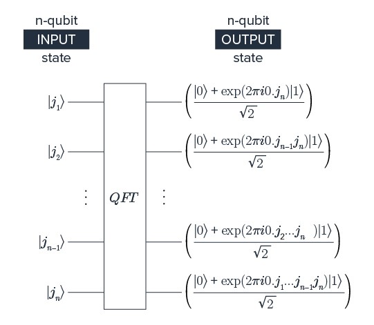
Figure 2.4: RSA Cryptosystem, Factoring, and Shor’s Algorithm Quantum Fourier Transform

2.7   Period Finding Algorithm

The quantum part of Shor’s algorithm is called “period finding.” In this section, we will discuss this quantum subroutine.

The period finding algorithm determines the period r of a periodic function $f\left(x\right)=f\left(x+r\right)$ from modular exponentiation. For example, to find the period of $f\left(x\right)=2^{x}\mod{15}$, we could test the function for different values of x from its smallest to its greatest value until we find the first x for which $f\left(x\right)=2^{x}\mod{15}=1\mod{15},$
$\displaystyle f\left(0\right)\displaystyle=\displaystyle 2^{0}\mod{15}=1,$
$\displaystyle f\left(1\right)\displaystyle=\displaystyle 2^{1}\mod{15}=2,$
$\displaystyle f\left(2\right)\displaystyle=\displaystyle 2^{2}\mod{15}=4,$
$\displaystyle f\left(3\right)\displaystyle=\displaystyle 2^{3}\mod{15}=8,$
$\displaystyle f\left(4\right)\displaystyle=\displaystyle 2^{4}\mod{15}=1,$
$\displaystyle f\left(5\right)\displaystyle=\displaystyle 2^{5}\mod{15}=2,$
$\displaystyle f\left(6\right)\displaystyle=\displaystyle 2^{6}\mod{15}=4.$

From here, we can realize that the function’s period is r=4 since the function’s values start repeating after x=4. However, for large numbers, finding this period is difficult to implement by hand, but it is also inefficient to find the brute force on a classical computer. However, Shor’s algorithm provides an alternative, efficient method.

The quantum period-finding algorithm uses two registers of qubits. The first register is called the source register, and the second one the target register. If the number to be factorized using Shor’s algorithm is N, then the number of qubits l in the first register has to satisfy

$$N^{2}\leq 2^{l}\leq 2N^{2}.$$ (2.41)

The number of qubits in the first register should generate a state-space that is at least large enough to capture the maximum possible period. The larger the value of ${l}$, the more densely the solution-space that can be sampled, and thereby, the error in determining the period can be reduced. For simplicity, the number of qubits in the second register will be ${l}$.

1. The qubits in the both registers start in the $\left|0\right\rangle$ state. The first step is to apply Hadamard gates to the source register to create a large, equal superposition state. This is equivalently sometimes called a QFT, although a QFT is much less efficient to implement in general than a single Hadamard on each qubit. Whether written as Hadamards or as a QFT, the operation transforms the state of the source qubits:

$$\begin{split}\left|0\right\rangle\otimes\left|0\right\rangle\otimes...\otimes\left|0\right\rangle\otimes\left|0\right\rangle\rightarrow\left(\frac{\left|0\right\rangle+\left|1\right\rangle}{\sqrt{2}}\right)\otimes\left(\frac{\left|0\right\rangle+\left|1\right\rangle}{\sqrt{2}}\right)\otimes...\\ ...\otimes\left(\frac{\left|0\right\rangle+\left|1\right\rangle}{\sqrt{2}}\right)\otimes\left(\frac{\left|0\right\rangle+\left|1\right\rangle}{\sqrt{2}}\right)\end{split}$$ (2.42)

which can also be written as

$$\left|0\right\rangle\rightarrow\frac{1}{\sqrt{2^{l}}}\sum_{x=0}^{2^{l}-1}\left|x\right\rangle,$$ (2.43)

where now $\left|0\right\rangle$ is in the l-qubit basis. This leaves the system in the state

$$\frac{1}{\sqrt{2^{l}}}\sum_{x=0}^{2^{l}-1}\left|x\right\rangle\left|0\right\rangle$$ (2.44)

2. The unitary operation $U_{f}$ is applied. This gate implements the modular exponentiation,$x\rightarrow f\left(x\right)=a^{x}\mod{N},$ such that the system ends in the state

$$\frac{1}{\sqrt{2^{l}}}\sum_{x=0}^{2^{l}-1}\left|x\right\rangle\left|a^{x}\mod{N}\right\rangle.$$ (2.45)

From here, we can see that the result of the period function $f\left(x\right)=a^{x}\mod{N}$ gets stored on the target register.

3. The second register is measured, and assume that this measurement projects the second register to the state $\left|f\left(x_{0}\right)\right\rangle=\left|a^{x_{0}}\mod{N}\right\rangle,$ where $x_{0}$ are the unique values of x in the first period of f(x) values.

Now, remember that a periodic function with period r only takes r different values. The function $f\left(x\right)$ is unique for distinct periodic values of x,

$$f(x_{0})=f(r+x_{0})=f(2r+x_{0})=f(3r+x_{0})=...=a^{x_{0}}\mod{N}$$ (2.46)

If the second register is projected to $\left|f\left(x_{0}\right)\right\rangle,$the first register will be in a superposition of the states $\left|x\right\rangle$ for which$f\left(x\right)=a^{x_{0}}\mod{N}$. For simplicity, Let us assume that there are $2^{l}/r$ different values of x for which $f\left(x\right)=a^{x_{0}}\mod{N},$ such that

$$f(x_{0})=f(r+x_{0})=f(2r+x_{0})=...=f\left(\frac{2^{l}}{r}r+x_{0}\right)=a^{x_{0}}\mod{N},$$ (2.47)

or

$$\sum_{y=0}^{2^{l}/r-1}f\left(yr+x_{0}\right)=a^{x_{0}}\mod{N},$$ (2.48)

with y an integer from 0 to $2^{l}/r-1.$ Once the second register is projected to $\left|f\left(x_{0}\right)\right\rangle,$ state of the system can be written as

$$\frac{1}{\sqrt{2^{l}/r}}\sum_{y=0}^{2^{l}/r-1}\left|yr+x_{0}\right\rangle\left|f\left(x_{0}\right)\right\rangle.$$ (2.49)

4. Even though the information of the period r is encoded in the first register, there is still one more step before being able to find its value. A (second) Quantum Fourier Transform is applied on the first register, this leaves the first register on the state

$$\frac{1}{\sqrt{r}}\sum_{z=0}^{r-1}\exp\left(\frac{2\pi i}{r}zx_{0}\right)\left|z\frac{2^{l}}{r}\right\rangle.$$ (2.50)

5. The first register is measured, projecting the l-qubit system to the state $\left|C\right\rangle,$ with $C=z2^{l}/r.$ Knowing the value of C implies knowing the value of the ratio

$$\frac{C}{2^{l}}=\frac{z}{r}.$$ (2.51)

If z and r have no common divisors, $\gcd\left(z,r\right)=1,$ the ratio $C/2^{l}$can be reduced to an irreducible fraction, as

$$\frac{C}{2^{l}}=a_{0}+\frac{1}{a_{1}+\frac{1}{a_{2}+\frac{1}{...}}}.$$ (2.52)

The approximations to the ratio z/r can be computed by using the continued fraction expansion relations:

$\displaystyle z_{0}\displaystyle=\displaystyle a_{0},$

$\displaystyle r_{0}\displaystyle=\displaystyle 1,$

and

$\displaystyle z_{n}\displaystyle=\displaystyle a_{n}z_{n-1}+z_{n-2},$

$\displaystyle r_{n}\displaystyle=\displaystyle a_{n}r_{n-1}+r_{n-2}.$

6. Different values for $z_{j}$ and $r_{j}$ are tested, until one finds values such that $\gcd\left(z_{j},r_{j}\right)=1$. For the valid values of $r_{j}$, the function $f\left(x\right)=a^{x}\mod{N}$ is evaluated with $x=r_{j}$. If $f\left(r_{j}\right)=1,$ then the period of f is $r_{j}$; otherwise, we have to go back to step 1.
To understand how this algorithm works, Let us find the period of the function $f\left(x\right)=11^{x}\mod{21}.$

We start by choosing the number of qubits in each register. For the first register, the number ${l}$ has to satisfy$21^{2}\leq 2^{l}\leq 2\times 21^{2}or441\leq 2^{l}\leq 882.$ Let us consider that each register has ${l}$ = 9 qubits.

1. All the qubits start in the ground state $\left|0\right\rangle.$ A Hadamard gate is applied on each one of the qubits on the first register. This transforms the state of the first register as

$$\left|0\right\rangle\rightarrow\frac{1}{\sqrt{2^{9}}}\sum_{x=0}^{2^{9}-1}\left|x\right\rangle.$$ (2.53)

This leaves the system in the state

$$\frac{1}{\sqrt{2^{9}}}\sum_{x=0}^{511}\left|x\right\rangle\left|0\right\rangle,$$ (2.54)

Where $\left|0\right\rangle$ represents the ground state of 9 qubits.

2. The unitary operation $U_{f}$ is applied, leaving the system in the state

$$\frac{1}{\sqrt{2^{9}}}\sum_{x=0}^{511}\left|x\right\rangle\left|11^{x}\mod{21}\right\rangle$$ (2.55)

$$=\displaystyle\frac{1}{\sqrt{2^{9}}}\left(\left|0\right\rangle\left|11^{0}\mod{21}\right\rangle+\left|1\right\rangle\left|11^{1}\mod{21}\right\rangle+\left|2\right\rangle\left|11^{2}\mod{21}\right\rangle\right)$$ (2.56)

$$+...+\left(\left|509\right\rangle\left|11^{509}\mod{21}\right\rangle+\left|510\right\rangle\left|11^{510}\mod{21}\right\rangle+\left|511\right\rangle\left|11^{511}\mod{21}\right\rangle\right)$$ (2.57)

$$=\displaystyle\frac{1}{\sqrt{2^{9}}}\left(\left|0\right\rangle\left|1\right\rangle+\left|1\right\rangle\left|11\right\rangle+\left|2\right\rangle\left|16\right\rangle+...+\left|509\right\rangle\left|2\right\rangle+\left|510\right\rangle\left|1\right\rangle+\left|511\right\rangle\left|11\right\rangle\right)$$ (2.58)

3. Assume the second register is measured, projecting it into the state $\left|f\left(2\right)\right\rangle=\left|16\right\rangle.$ This leaves the first register in

$$\frac{1}{\sqrt{2^{9}/r}}\sum_{y=0}^{2^{9}/r-1}\left|yr+2\right\rangle\left|16\right\rangle$$ (2.59)

$$=\displaystyle\frac{1}{\sqrt{2^{9}/r}}\left(\left|2\right\rangle+\left|r+2\right\rangle+\left|2r+2\right\rangle+...+\left|\left(\frac{2^{9}}{r}-1\right)r+2\right\rangle\right)\left|16\right\rangle$$ (2.60)

4. A Quantum Fourier Transform is applied on the first register such that

$$\frac{1}{\sqrt{2^{9}/r}}\sum_{y=0}^{2^{9}/r-1}\left|yr+2\right\rangle\left|16\right\rangle\rightarrow\frac{1}{\sqrt{r}}\sum_{z=0}^{r-1}\exp\left(2\frac{2\pi i}{r}z\right)\left|z\frac{2^{9}}{r}\right\rangle.$$ (2.61)

5. Assume the first register is measured, projecting it into the state $\left|427\right\rangle$. The irreducible fraction of the ratio $C/2^{9}$ is given by

$$\frac{C}{2^{l}}=\frac{427}{2^{9}}=0+\frac{1}{1+\frac{1}{5+\frac{1}{42+\frac{1}{2+\frac{1}{...}}}}}.$$ (2.62)

Note that we can calculate this irreducible fraction in Wolfram Alpha by typing in the bar “continued fraction of 427/512.”

6. The values $z_{j}$ and $r_{j}$ are tested for the condition $\gcd\left(z_{j},r_{j}\right)=1$ with j from 0 to 3,
$\displaystyle\gcd\left(z_{0},r_{0}\right)\displaystyle=\displaystyle\gcd\left(0,1\right)=1,$
$\displaystyle\gcd\left(z_{1},r_{1}\right)\displaystyle=\displaystyle\gcd\left(1,1\right)=1,$
$\displaystyle\gcd\left(z_{2},r_{2}\right)\displaystyle=\displaystyle\gcd\left(5,6\right)=1,$
$\displaystyle\gcd\left(z_{3},r_{3}\right)\displaystyle=\displaystyle\gcd\left(427,512\right)=1.$

The function $f\left(x\right)=11^{x}\mod{21}$ is evaluated for different valid values of $r_{j}$,
$\displaystyle f\left(1\right)\displaystyle=\displaystyle 11^{1}\mod{21}=11$
$\displaystyle f\left(6\right)\displaystyle=\displaystyle 11^{6}\mod{21}=1$
$\displaystyle f\left(512\right)\displaystyle=\displaystyle 11^{512}\mod{21}=16$

With this result, we can conclude that the period of the function f is r=6.

2.8   Shor’s Algorithm: Reduction of Factoring to Order Finding

In the next text units, we will take a deep dive into several details behind Shor’s algorithm, including a discussion of the reduction of factoring to order finding, the related Simon’s algorithm that helped inspire Shor’s algorithm, and the use of Shor’s algorithm to perform order finding.

How do we get factoring from order finding? So, first, let say the second-fastest classical algorithm is the quadratic sieve. So, we would say most classical algorithms[77]. So, suppose we have N equals P times Q. They work in more general cases, but we will just worry about the case of two products. So, the first step, really the only step, the trick is to find x squared congruent to y squared mod N x not congruent to plus or minus y mod N. So, suppose we are trying to factor 21. we get 4 is congruent to 25 mod 21, right? Because 25 minus 4 is a multiple of 21. So, 4, these are both squares. Moreover, now we have 5 minus 2 times 5 plus 2 is congruent to zero mod 21. whenever this happens, one of these contains P, and the other contains Q. Or rather, whenever neither of these is 0, we have a product of two numbers, which is zero mod 21. Thus, we know that the product has to contain three somewhere, and it has to contain somewhere. If neither of these factors is 0 mod 21, 3 has to be contained in one factor and 7 in the other. Then, what we can do is we can use Euclid’s algorithm for GCD to get P and Q. So, we are essentially done whenever we get two squares, which are equal to each other. This is how the quadratic sieve works. That is the second-fastest classical factoring algorithm known. How do we find x squared y squared? Well, let us look at the function f of x equals g to the x mod N. So, this is periodic. If g to the r is congruent to 1, then g to the x plus r is congruent to g to the x mod N. Because if g to the r plus is congruent to 1, then g to the x plus r congruent to g to the x because it is just multiplying both sides of this by g to the x. So, that says that f of x is periodic. We mean, it has to start repeating some time because there are only N possible things here. Whenever it starts repeating, we get a g to the x plus r congruent to g to the x. that means g to the r is congruent to 1. g to the r over 2 squared is congruent to 1 squared if r is even. So, let us do an example. Suppose we are trying to factor 21. So, 2 to the 0, 2 to the first, 2 squared. So, this is 1, 2, 4, 8, 16, 32. 32 minus 21 is 11, so, the next column then is 11. 22 minus 21 is 1. 1. So, 2 to the sixth is congruent to 1 mod 21. That means 2 cubed minus 1 minus time 2 cubed plus 1 is congruent to 0 mod 21. this is 7, and this is 9. 7 contains the factor 7, 9 contains the factor 3. So, the question is, how can this go wrong? Moreover, well, there is a couple of things that could go wrong. We could have started with 4. 4, 16. 16 squared, well, we know 2 to the sixth is congruent to 1 mod 21. So, 4 cubed is congruent to 1 mod 21. So, we get 4 cubed is congruent to 1 mod 21. 4 to the 3/2 does not exist. Well, we cannot compute it. So, this shows that 4 could go wrong. The only thing that could go wrong is we could do this. When we look at the middle element, it is minus 1. that would be a problem because then we have x is equal to minus y mod N. we cannot use that, we cannot use this trick then. So, some things can go wrong, but the great theorem is the probability of success with g to the xth is greater than or equal to 1/2 for a random g between 0 or a random g less than N. So, we choose a random g less than N. we do this repeated squaring. The probability this will work is at least 1/2. If it does not work, we choose another random g. So, eventually, with high probability, we will get a g, which lets us factor.

2.9    Introduction to the Shor Quantum Factoring Algorithm

we discovered the factoring algorithm after seeing Simon’s algorithm before Simon’s algorithm got published. We are going to show we write down a circuit diagram so we can see the similarity. So, Simon’s algorithm, remember, we started with n qubits in the plus. Then we went, and here is a black box that computes 0 to the n. From x, it computes f of x. then we did a Hadamard transform to the n, which is just the quantum Fourier transform over the group of two elements to the n-th power. So, n copies of the group of two elements. So, this is just binary strings under addition without carries. After that, we believe we measured this register, and then did classical post-processing. So, what is factoring? So, what we are not going to do directly is a quantum algorithm for factoring. We are going to do a quantum algorithm for an order finding a quantum algorithm for periodicity. So, suppose we have a function over integers, f of x is equal to f of x plus c for some c. here we can see that f of x 2c equals f of x plus 3c. So, it is a periodic function, and a period is well, we call it C right now, but at some point during this section, we are going to start calling it r because that is what we used to call it. Find c. Now we might think this is easy. We just start with f of 0, f of 1, f of 2, f of 3, and keep on going until f starts repeating. So, even if the period is exponentially long. That means that if we want to try to find a period of length r, we can do this length polynomial and log of r. So, we can find the period. On the classical computer, if we have a black-box function, the best thing we can do is to keep on testing values until it starts repeating. So, that means the best we can do is period r. in quantum mechanics, quantum computing, we can do log r. So, it is going to be exponentially long in a period of a number we want to factor. However, if we are just finding a period, find a period in time O of log c. So, we will be able to find the period and time well, that is going to be quicker than log c if we want to do it quicker. Log c squared if we want to do it quickly because we cannot use the exact quantum Fourier transform, but the approximate quantum Fourier transform, which has like log c, log log c gates But here, so, we want to find a period. We have a black box function for f. f has some period of c. So, what is the quantum algorithm for this? Well, we are going to do the same thing here. We are going to start at plus to the c, 0, the n here. Here we have a black-box function, which, if we put in x, computes f of x. Alternatively, actually, it computes well, remember this took x, t to x, t xr f of x. we can assume this does the same thing. x, t to x t xr f of x. nowhere is the only difference, really, between the circuits. We use the quantum for each transform over 2 to the actual, let us do this right. There is 2n. We want 2n qubits, n qubits here. Quantum Fourier transforms over 2 to the n. then we measure. Then we do classical post-processing. So, it looks very similar. So, let us go into detail, in both these cases, what happens to the bottom branch? We do nothing to the bottom branch. We mean that we could measure the bottom branch and throw away the results if we want to. Alternatively, we do not have to. If we measure something and throw away the results, it does not matter whether we measure it. However, we do need to compute it. Because if we do not compute it, what have we done? We have taken the Hadamard transform of x to the n. That is just all 0’s. So, if we do not compute f of x, it destroys the interference in the upper half. Again, action in a quantum circuit has back action.

2.10   Simon’s Algorithm

In 1994, Daniel Simon posed the following question: Does a particular function map distinct input elements to unique output elements hence representing a permutation or a one-to-one mapping function or, does it follow a two-to-one mapping scheme? Despite the problem’s small practical importance, it is a quantum algorithm that exhibits an exponential speedup. Simon’s algorithm served as an inspiration for Peter Shor and his famous quantum algorithm for period finding.

Simon’s algorithm addresses a particular black-box function $f:\{0,1\}^{n}\rightarrow\{0,1\}^{n}$, which is known to map inputs in either a one-to-one or two-to-one manner. Two distinct input bit strings $a_{1},a_{2}\in\{0,1\}^{n}$ are mapped to the same output $f(a_{1})=f(a_{2})$ if:
1. the two bit strings $a_{1}$ and $a_{2}$ are equivalent a one-to-one function, or
2. there exists a bit string $s\neq 0^{n}$such that $a_{1}\oplus s=a_{2}-a$ two-to-one function.

If there exists a single $s\neq 0^{n}$, the mapping is “two-to-one” and otherwise (if $s=0^{n}$ works) it is “one-to-one”. Simon’s algorithm finds the bit string s and the type of function mapping exponentially faster than known classical algorithms.

The algorithm starts with the initialization of 2n qubits in their ground state. Subsequently, half the qubits are rotated with a Hadamard gate to form an equal superposition state.Thereafter, the oracle function $U_{f}$ is applied on all qubits. A second Hadamard gate is applied to the same qubits that received the first Hadamard gate, and then then qubits are read out. The mathematical description of the protocol can be formulated as follows:

$$\begin{split}\lvert 0\rangle\dots\lvert 0\rangle=\lvert 0^{n}\rangle\lvert 0^{n}\rangle\leavevmode\nobreak\ \leavevmode\nobreak\ \leavevmode\nobreak\ \xrightarrow{H^{\otimes n}I^{\otimes n}}\leavevmode\nobreak\ &\frac{1}{\sqrt{2^{n}}}\sum_{a\in\{0,1\}^{n}}\lvert a\rangle\lvert 0^{n}\rangle\\ \xrightarrow{\leavevmode\nobreak\ \leavevmode\nobreak\ \leavevmode\nobreak\ U_{f}\leavevmode\nobreak\ \leavevmode\nobreak\ \leavevmode\nobreak\ }&\frac{1}{\sqrt{2^{n}}}\sum_{a\in\{0,1\}^{n}}\lvert a\rangle\lvert f(a)\rangle\\ \xrightarrow{H^{\otimes n}I^{\otimes n}}&\frac{1}{2^{n}}\sum_{b\in\{0,1\}^{n}}\sum_{a\in\{0,1\}^{n}}(-1)^{a\cdot b}\lvert a\rangle\lvert f(a)\rangle\\ \text{if }f(a_{1})=f(a_{2})\rightarrow a_{1}\oplus s=a_{2}:\leavevmode\nobreak\ \leavevmode\nobreak\ \\ \frac{1}{2^{n}}\sum_{b\in\{0,1\}^{n}}\sum_{a_{1}\in A}((-1)^{a_{1}\cdot b}+(-1)^{a_{1}\oplus s\cdot b})\lvert a_{1}\rangle\lvert f(a_{1})\rangle\\ \frac{1}{2^{n}}\sum_{b\in\{0,1\}^{n}}\sum_{a_{1}\in A}(-1)^{a_{1}\cdot b}(1+(-1)^{s\cdot b})\lvert a_{1}\rangle\lvert f(a_{1})\rangle\\ \text{summands\leavevmode\nobreak\ }\neq 0\text{\leavevmode\nobreak\ \leavevmode\nobreak\ only if\leavevmode\nobreak\ }s\cdot b=0:\leavevmode\nobreak\ \leavevmode\nobreak\ \\ \frac{1}{2^{n-1}}\sum_{b\in\{0,1\}^{n}\leavevmode\nobreak\ \&\leavevmode\nobreak\ s\cdot b=0}\sum_{a_{1}\in A}(-1)^{a_{1}\cdot b}\lvert a_{1}\rangle\lvert f(a_{1})\rangle\end{split}$$ (2.63)

The detectable states non-zero coefficients fulfill the condition of $s\cdot b=s_{1}b_{1}\oplus\cdot\cdot\cdot\oplus s_{n-1}b_{n-1}=0$ a dot product modulo 2. To determine s with high accuracy it is necessary to repeat the algorithm to acquire n-1 linearly independent $b_{1},\dots,b_{n-1}$. Upon repeated runs of the algorithm, equations $s\cdot b_{1}=0,\dots,s\cdot b_{n-1}=0$enable a classical calculation of the solution $s^{\prime}$. If$f(s^{\prime})=f(0^{n})$ holds, the black box function maps its input states in a two-to-one manner. In contrast, if $f(s^{\prime})\neq f(0^{n})$ with $s^{\prime}\neq 0^{n}$, the derived $s^{\prime}$ is not a valid solution. Therefore, only $s=0^{n}$ satisfies $f(s^{\prime})=f(0^{n})$ and the function is one-to-one. Simon’s algorithm is optimal and yields an answer after $\mathcal{O}(n$) queries. In contrast, a classical algorithm requires at least$\mathcal{O}(2^{n/2})$ queries.

Both Simon and Shor’s algorithms are related to finding the order or the period of a function of interest. In Simon’s algorithm, this is accomplished through quantum interference induced by Hadamard gates and multiple measurements. In Shor’s algorithm, the period finding is accomplished using the quantum Fourier transform.

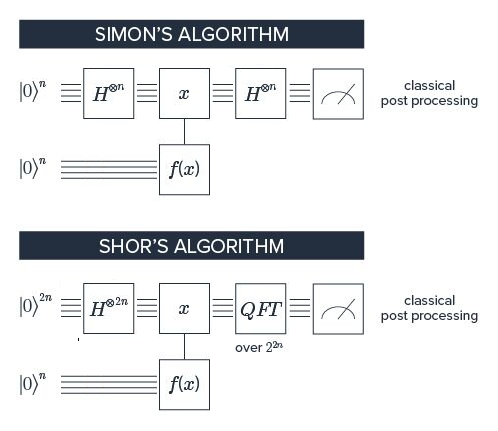
Figure 2.5: SS Algorithm

2.11   Shor’s Algorithm: Detailed Steps of the Quantum Order Finding Algorithm

What is the algorithm in detail? So, suppose we have a bound-on r we should call it r-max and choose a power of 2 bigger than 2 r-max. Well, we will write down the algorithm. We start with plus to the 2l 0. That is here. Next, we take the compute f with x. We know that whatever ends in the first register, we compute it in the second register. However, this is just sum i equals 0 to 2 to the 2l. i, where i is just the binary representation of the number. We need to divide by 2 to the l because we want this to be a unit vector. So, we compute f. So, this becomes sum to the 2l i f of i. i equals 0 to 2 to the 2l. Do the quantum Fourier transform. So, that is 1 over to 2 to the 2l summation. We know i is a really bad letter to use because it is also the square root of minus 1. So, let us use x. So, the quantum Fourier transform takes x to, let us call it, z f of x. z equals 0 to 2 to the 2l minus 1. e to the 2 $\pi$ i xz over 2 to the 2l. So, we have taken x and taken the Fourier transform of it, which gives us this. Now, what happens if we measure f of x? well, we are going to get some value for f of x. we are going to leave that out the normalization constant for the time being because figuring out exactly What is going on with a normalization constant is possible, but it is much tedious algebra. We will come back to it later. So, without a normalized, z equals 0 through 2 to the 2l. Let x0 be the smallest x giving f of x. So, this is going to be z of the form x0 plus y times $\pi$. Because when we measure f of x, we only get z no, not z. When we measure f of x, we only get x equals x0 plus yr f of x0 z e to the 2 minus 2 $\pi$ i x well, xz, but x is of the form x0 plus yrz over 2 to the 2l. So, what did we do? We measured f of x here. We are just looking at the ones who give us f of x0. We know all of these x’s are the form x0 plus yr. The phase factor does not change, and z does not change. So, now we have the sum. We have to figure out how big it is. Well, we can write sum z equals 0 through 2 to the 2l. Sum y equals 0 through 2 to the 2l over r, plus or minus 1 here, but that does not matter. f of x0 z e to the 2 $\pi$ i x0 plus yrz over 2 to the 2l. What is this? This is a geometric sum.

2.12   Shor’s Algorithm: Order Finding Algorithm Measurement Result as a Geometric Sum

So, first, we will do the intuition, and then we will do the math. So, it is a geometric sum, and it is a whole bunch of points around the unit circle. So, we start with e to the minus 2 $\pi$ i x0. Let us plot these points minus 2 $\pi$ i x0. now we go r, z over to the 2 to the 2l. So, the next one we want to plot is y equals 1. So, we go some distance around the circle. Let us plot another point. Then we plot another point, another point, another point. We keep ongoing. What we get is quite possibly points that are exactly uniformly distributed over the unit circle, sum close 0. well, and next, what happens is, here was e to the 2 $\pi$ i x0 2 to the 2l. Here is e to the minus 2 $\pi$ i x0 plus rz zero over 2 to the 2l. So, unless what happens is when we plot the point, we move around by the angle 2 $\pi$ i rz over 2 to the 2l. Suppose this angle is tiny. Well, what happens then is we get points uniformly distributed. Suppose it is tiny enough so, that when we add all of these 2 to the l over r points, we get points that are we know, some kind of an arc, which does not even go all the way around the unit circle sum is close to well, how many points were there? There were 2 to the 2l over r. they were all pointing in more or less the same direction. So, an absolute value. So, there are two cases here. 2 $\pi$ i yr If 2 $\pi$ i rz over 2 to the 2l is close to 1, which means y rz over 2 to the 2l is close to an integer. Let us call that integer d. So, if this is close to an integer, then we get a large probability of seeing this. If it is not close to an integer, we get a tiny probability of seeing it. So, the geometric sum is 1 minus e to the 2-$\pi$ i. we want the last term of the sum. So, that is 2 to the 2l rz over 2 to the 2l. No, it is y goes from 1 to 2 to the 2l over r. So, the last term we substitute in 2 to the 2l r over z. So, something like 2 to the 2l over r. we will have to take the floor of that time r times z over 2 to the 2l. Which really, because of this floor could be anywhere on the unit circle. However, it is always less than 2 in absolute value. We are dividing that by 1 minus e to the 2 $\pi$ i rz over 2 to the 2l. Remember, the sum is, so we are dividing something by something else. It is going to be relatively small unless something else we are dividing is close to 0. So, this is roughly something O of 1 divided by oh, what is this? This is rough rz over 2 to the 2l. The probability of seeing a number z is rough rz over 2 to the 2l squared minus d because d was the integer. So, we have d over r is roughly z over 2 to the 2l. So, what the algorithm does is it output z. we know 2 to the 2l, and we need to round it off to something like d over r. there is a procedure for rounding real numbers of two smaller fractions that is efficient. It is called continuous fractions. However, it is a classical algorithm. So, once we get this, we can round it to d over r, and then we are found r, which was the period we were looking for.

2.13   Demonstrations of Shor’s Algorithm: Introduction

In the next several sections, we will explore two demonstrations of Shor’s algorithm on small-scale quantum-computers realized using liquid-state NMR and trapped ions. Although the numbers of qubits and the number being factored is rather small (15 = 3 x 5), the demonstrations illustrate that Shor’s algorithm works in principle. We will also discuss how many demonstrations have used “compiled” versions of Shor’s algorithm that are not generalizable.

To date, there have been a handful of prototype demonstrations of Shor’s Algorithm using different qubit modalities, including nuclear spins, photonic qubits, superconducting qubits[185], and trapped ions. In this section, we will look at two of these demonstrations in detail. The first is a demonstration of Shor’s Algorithm using liquid-state nuclear magnetic resonance, NMR. This was, in fact, the first such experimental demonstration, and it showed the factorization of 15 into the primes 3 times 5. It used molecules with seven individually addressable nuclear spins in a liquid solution at room temperature, and the algorithm comprised a sequence of around 300 pulses. we will discuss this work. The second demonstration is recent, and it was performed using trapped ions [250]. In this case, seven ions were used to again factor the number 15 into primes 3 and 5. In this example, modular multiplication was implemented, and no simplifications presumed prior knowledge of the result were employed. Instead, a concept called qubit recycling was used to make up for the fact that seven qubits are insufficient to implement the general algorithm. Still, to date, this demonstration constitutes the most realistic implementation of Shor’s Algorithm. MIT Professor Isaac Chuang participated in this demonstration with Professor Rainer Blatt’s team at Innsbruck. To factor 15 in a straightforward manner, it is estimated that one needs about 12 qubits, eight qubits in the period register, and four qubits in the modular multiplication register. The demonstrations we will discuss in this study had fewer than 12 qubits, and so, certain simplifications had to be made. Now in many cases, the simplifications were quite reasonable. For example, the use of qubit recycling. Nonetheless, it is important to understand the impact of various types of simplifying assumptions. Finally, from a business perspective, these prototype demonstrations of Shor’s Algorithm illustrate that quantum computing is real. Although these implementations are not yet at scale, they are concrete indications of and steps towards the promise of quantum computing. From an engineering perspective, these types of demonstrations force groups to confront practical realities of implementation, from qubit control engineering to algorithmic compilation. Although not yet at scale, these algorithms motivate experimental groups to go beyond scientific demonstrations and to meet face-to-face with the practical realities that will need to be accommodated to enable scalable quantum computing. scientifically, these demonstrations test the knowledge of system noise [126, 150] and decoherence [117]. Lastly, from a technology standpoint, these demonstrations serve as a benchmark of progress in the field, indicating where the technology currently stands and clarifying what needs to be addressed in order to reach future milestones. With that brief introduction, let us discuss.

2.14   Demonstrations of Shor’s Algorithm: Shor’s Algorithm with NMR

In 1998, after implementation of the first two-qubit algorithms on the chloroform molecule and using NMR, Isaac Chuang, who supervised the research, gave a great challenge to factor the number 15 within the time span of Ph.D. at Stanford. At that time, Isaac Chuang was transitioning from Los Alamos National Laboratory to the IBM Almaden Research Center outside San Jose. He was finishing the first year of Ph.D. at Stanford. At that time, Isaac set up his new lab at Almaden, some 30 minutes away from Stanford. Researcher did not know what it would take to factor the number 15, but it did seem like a great challenge. certainly, it was clear that there was an enormous interest in Shor’s Algorithm and that it was a major driver for the field. So, we thought it would be very awesome to demonstrate Shor’s Algorithm experimentally. So, what would it take to run Shor’s Algorithm experimentally? The simplest instance of quantum factoring is to factor the number 15, to pull it apart into 3 times 5. However, how many qubits does that take, and how many operations? we got great insight from a pedagogical article by Dave Beckman from the Preskill group at Caltech. In particular, he analyzed the steps for factoring the number 15. Shor’s algorithm, in general, consists of two parts, a classical part and the quantum mechanical part. The quantum part that we run on the quantum computer is designed to find the period of a function, specifically the function a to the power x modulo N, that is to say, the remainder after division of a to the x by N. N here is the number we are trying to factor. A number can be anything as long as it is co-prime with N, and x is the function’s argument. For period finding on a quantum computer, we divide the number of qubits into two registers. One register needs to be large enough that it can store the number N. For 15, we need four bits, so, four qubits are needed for that register. The other register, in principle, needs to be twice as large or eight qubits, bringing the total to 12 qubits to factor the number 15. The algorithm consists of, first, a Hadamard operation that prepares an equal superposition of all the states of the first register then a function call of the function a to the x modulo N where x is the states of the first register. the result is mapped into the state of the second register. the third step is the Quantum Fourier Transform applied to the first register. At the end of the computation, we read out this first register. Now, if we begin to analyze how to implement this complex function a to the x modulo N, we realize that it can be broken apart into multiple simpler operations. Each of them is an operation controlled by just one bit out of all the bits of the first register. then we find for the number 15 that we are lucky. Only two of the control qubits play a role in factoring 15. in some cases, some choices of a, even just one of the control qubits, plays a role. So, that allows us to eliminate many qubits of the first register. In principle, we could eliminate all of them except two. We decided that for a meaningful Quantum Fourier Transform, we would like to have not just two qubits but three qubits. With two qubits, the Quantum Fourier Transform comes down to a single two-qubit gate. we thought that was too trivial. So, in the end, we went with an experiment with a total of seven qubits to factor the number 15. So, in NMR, the qubits are represented by the nuclear spins in the molecule, the spins of the atomic nuclei in a molecule. For a successful molecule for NMR qubit experiments, the molecule needs to have rather unusual properties. we need what we call large chemical shifts. That is to say, large separations in frequency between all the spins we want to get involved in the computation for selective addressing of the qubits. nd we want a coupling network that allows sufficient pairs of qubits, pairs of spins, to be coupled to each other so that all the required two-qubit gates can be implemented on the molecule. So, a staff member at IBM Almaden did an extensive search looking through fast tables and documents with tabulated NMR properties of known molecules. after spending days in this process, he concluded that none of the tabulated molecules were good enough for the experiment that were attempting. However, there was one that came close. It consisted of a backbone of four carbon atoms. surrounding it, there were five fluorine atoms that all could serve as a spin one-half and provide a qubit. besides, there was an iron complex. The iron complex created asymmetry in the molecule so that the resonance frequencies of the five fluorine atoms would be separated. To go from five fluorine spins to seven, what we needed to do was to isotopically label two of the carbon spins so that they became carbon-13 and also acquired a spin one-half. Synthesizing this molecule was a real tour de force. Greg Breyta, IBM staff member who usually worked on chemical synthesis in the Resist program, spent over one year trying to synthesize this molecule. at any point in time in this multi-step synthesis, they did not know if this next step would be successful. However, finally, after more than a year, actually just in time, when they were ready to try the experiment, he delivered the molecule. So, the next challenge was to develop the control techniques to take the seven spins through the steps of Shor’s Algorithm, to make them do the spin dance with a great degree of control. Here we could benefit from decades of technology development in NMR spectroscopy, where people were interested in revealing the structure of molecules they were synthesizing. Mark Sherwood done great work on NMR spectroscopy at IBM. In the years that followed in 1999 and 2000, we did experiments with the first two, then three, and five spins to discuss how to control the time evolution of increasing spins. They were all coupled together. Nevertheless, the factoring experiment became clear beyond anything that anyone had ever done in terms of controlling many coupled quantum spins. It required more than 300 radio frequency pulses, specially tailored in amplitude and phase, to allow selective addressing of each of the seven spins. Also, we had to account for unintended phase shifts that occurred on any of the qubits when we drove any other qubits. In addition to that, since we were competing against the decoherence timescale, we had to apply simultaneous rotations where crosstalk effects were even more severe. we had to account for those as well. then finally, in NMR in these molecules, the couplings are always on. So, we had to use some sophisticated so, called decoupling sequences that effectively remove the effect of all the couplings except the one coupling that we needed to run a two-qubit gate between two spins. So, together with Matthias Stephan, fellow Ph.D. student at Stanford, who started one year after, they went out to try and control the seven spins, starting in September of 2000. throughout that fall and the winter of 2001, they made much progress. they used a variant NMR four-channel spectrometer to control the seven spins. after some time, they were far enough that the output spectra revealed the information about the period of a to the x modulo 15. from that, they could say that they had factored 15. At the same time, they were disappointed because the output spectra, even though they did give us the right information, they did not look like what ideally expected. even though they added more and more sophistication in the control techniques, it seemed like they were hitting a wall. At some point, they set out to write a model to capture the main effects of decoherence simply. there it was, beautifully reproducing the experimental spectra, the simulated spectra accounting for decoherence. It was interesting because, in the four years of experience programming NMR sequences and operating on molecules, this was the first time that decoherence had become the limiter. The relationship between duration, strength, and phase of our pulses and their ultimate effect on rotations? so, we can think of operations on a single qubit in terms of a Bloch sphere, or the planet earth, and so we call the North Pole the ground state, state zero. We call the South Pole state one, and those are just classical states, zero, one. But anywhere else on the Bloch sphere, or think of it as planet earth, anywhere else on the earth, we are in a superposition of zero and one. so, we can perform rotations by applying resonant pulses to the qubit, and that will effectively rotate this Bloch vector around the planet earth. So, Let us say we start at the North Pole, and if we, so first we will discuss about duration and strength of the RF pulses. Basically, the amount of rotation we going to get is the area under this pulse. So, it is both the duration, as well as the amplitude of the pulse that matters. Now, we often apply a Gaussian-shaped pulse, or some kind of smoothly-shaped pulse. But if we think of it as a rectangle, then it is very easy to just say, look, it is the duration of the pulse, times the amplitude of the pulse, and we can rotate a given amount of degrees around a certain axis, and we can do that for a short, poll pulse, or we can do that for a very long pulse that is got a low amplitude. As long as they have the same area, we going to rotate the same amount. If we want to rotate further, similarly, we can increase the amplitude more, or we can keep the amplitude fixed, and increase the duration more. So again, it is the area under the pulse that matters, that is going to determine how far we rotate around the Bloch sphere. so, one of the first things that an experimentalist will do is calibrate their pulses, and part of what that means is understanding what duration and amplitude do we need to rotate 90 degrees? And what do we need to rotate 180 degrees? so that has to do with the amount of rotation. Now the second question is, what axis am we rotating around? And so, the, if we think of the, equator around the Bloch sphere, or around the earth, we can put an x and a y axis on here. so x is going to point in one direction, and y will be 90 degrees away from that, pointing in a perpendicular direction. there is plus and minus x, and there is plus and minus y. Now, when we apply this microwave pulse, we can generate that pulse using IQ mixing. so we means in-phase, Q means quadrature, and basically, what this allows us to do is output a pulse where the microwave tone that is resonant with our qubit transition is[164, 165], has zero phase shift with respect to the source, that would be the end phase channel. Or, we can use the quadrature channel, and output same pulse shape, but with the microwave shifted within that envelope by 90 degrees, And when we use the in phase, the in phase port, then what we will do is we will rotate around the x-axis. when we use the quadrature port, which shifts the microwaves by 90 degrees, we will rotate around the y-axis. so that is basically how the phase of the RF pulses will effect the rotation. It determines what axis these rotations are going to occur around. Now we might say, how do we know what is the x-axis to begin with? It turns out that there is always this relative phase offset that people discuss about. it is a little bit of jargon but, in quantum mechanics, and so, what sets the x-axis, basically, is our first pulse, right? So if our first pulse, Let us say it is got zero phase, we will rotate around a given axis. That axis becomes our x-axis, right? And everything relative to that, now, is either in-phase with that, or in quadrature with that, and if it is in-phase, we will rotate around that axis, and we call it x, and if we are in quadrature with that, we will rotate around the y-axis.

2.15   Demonstrations of Shor’s Algorithm: Perspective on NMR

So, let us reflect on what made this experiment successful. The first is that the coherence times, the t2’s in this specially designed molecule, were exceptionally long all more than 1 second. We have to compare, the coherence time to the time scale of the operations that form a single qubit-shaped pulse here varied between 0.2 and 2 milliseconds. We also have to compare to the value of the coupling strings between the spins in the molecule. They varied from about a hertz, which was too low to be usable, to about 200 hertz. In total, the longest sequences we had to run to implement Shor’s Algorithm lasted about 700 milliseconds. The second success factor is that in these experiments, we used liquid state NMR based on ensembles of many copies of a molecule, making the detection trivially easy, almost, compared to the great challenge of trying to work with individual spins as is done today. Furthermore, the liquid state NMR Hamiltonian is relatively transparent and simple. All the terms in the Hamiltonian commute with each other. Single qubit terms have to form omega times $\sigma$ z. the two-qubit interactions have to form J times $\sigma$ z on one qubit and $\sigma$ z on another qubit. Scaling this approach, however, is hard. First, we have already commented on the difficulty of finding a suitable molecule with seven spins. Moreover, finding molecules with larger numbers of qubits, with larger numbers of suitable spins, to solve more complex problems quickly gets extremely difficult. However, there is a more fundamental and severe limitation to the liquid state NMR approach, and it is that even though we work in large magnetic fields, the fact that we use liquid states pushes us to work at large temperatures. We operated at room temperature. Nuclear spins in a magnetic field at room temperature are in a highly mixed state, that is to say, the probability for a spin to start in the upstate or the downstate are almost equal. We used techniques developed in the community to prepare so-called, effectively pure states. These are states that produce a signal that is proportional to that of a pure state, but the cost of this technique is that the signal is halved for every qubit that we add. Thus, this induces exponential cost that offsets any exponential gain that we hope to get from the quantum algorithms [251]. The NMR experiments, and in particular the short experiment, had been great fun. Furthermore, we think we discussed a great deal from it that also benefit and still benefits, today, the community. However, certainly, we wanted to move to technology, where the potential for scaling was far better. We decided to move from nuclear spins to electron spins and from molecules to artificial molecules. The artificial molecules we make use of are built from Silicon quantum dots in which we can find individual electrons and use their spins as qubits[151]. Similar to the NMR molecules, these electron spins in silicon offer long coherence times[116], but the devices are much more scalable, and the control, in the end, can take us much further. Matthias Stephan, instead, chose to work on superconducting qubits, and he was one of the early members of the IBM team working on superconducting qubits, a very large and successful program today. Isaac Chuang finally decided to move to trapped ions. He set up a lab at MIT, and in collaboration with the group of Reiner Blatt Some years later. They redid the factoring experiments a beautiful experiment implementing the factoring of 15 on trapped ions. As for the silicon spins that we work, we set state of the art earlier this year in implementing for the first time, in this type of system, again, a two-qubit algorithm. It brought back great memories from ’98. However, different from the NMR approach and these early memories, the expectation is that with the group at QuTech in Delft and close collaboration with Intel, with the silicon spin qubits, we can go much beyond factoring 15.

2.16   Demonstrations of Shor’s Algorithm: Quantum Factoring With Trapped Ions - Ion Trapping System

Shor’s quantum factoring algorithm has been implemented by several physical systems, including trapped ions. Let us consider what was done and why. Perhaps the most important starting point is to consider the question, what is the smallest meaningful instance of the Shor quantum factoring algorithm? Recall that the intent of Shor’s factoring algorithm is to compute the period of this function, f of x equals a to the x mod N. In this expression, N is a number we wish to factor. x is the argument to the function. a is a random number, which is chosen that co-prime to N. It shares no prime factors in common with N. The period of this function, r, allows us to find with some probability, a high probability, a factor of N, which is non-trivial. Quantum factoring, thus, has as a goal finding this period, r. Solving this problem takes an amount of time, or several operations roughly proportional to L cubed where L is the number of digits of the number N. Classically, using the best-known algorithm, the time required, or several operations required roughly go as e to the L/3. The difficulty of this factoring problem is at the root of what secures widely used cryptosystems, such as RSA. To appreciate the smallest meaningful instance of Shor’s quantum factoring algorithm, it is helpful to review the quantum circuit for the algorithm. Recall that there are two registers, the top one here, which holds the value x in a superposition of all possible values, and a bottom register, where the result of the modular exponentiation is held. The top register is then fed three inverse Quantum Fourier Transform, which returns the result. There are three main steps in this procedure. First, the input superposition of the top register must be created. Second, the modular exponentiation, a to the x mod N, must be computed. It is the most difficult part of Shor’s quantum factoring algorithm because multi-qubit gates are required. The third step is a Quantum Fourier Transform. because the result of the Fourier transform is measured, only single-qubit gates, some of them controlled by classical results, are required in principle. After the result is measured, there are some classical post-processing. this can be done by essentially any classical computer. Now, the number we are factoring is N., And it is clear that the algorithm is too trivial when N is an even number. That is, it has a factor, which is 2. Thus, the smallest meaningful factors are 3 and 5. Here is a generic quantum factoring circuit for the case of N equal 15, namely 3 times 5. What makes this specific for N equal 15 is the choices available for the random base to be chosen, a. a must be co-prime with N. In other words, it must not discuss any factors with N. it must be less than N. Therefore, the only two meaningful cases are a being 7 and 11. Thus, the modular exponentiation circuit in the middle reduces to looking like this, where we have used repeated squaring as it is common to realize the modular exponentiation. Note that each one of these exponentiations is calculated mod 15. So, we began with a controlled multiplication by a, then a controlled multiplication by a square, a to the fourth, a to the eighth, a the 16th, and so, forth, all the way up to a to the 128th power. the result of each of these multiplications is still a number between 0 and 14 because of the modular multiplication being performed. So, two non-trivial values of a may be used in factor 15. we claim that one of these is easy to handle, and the other is hard. Why is this the case? well, let us see why by working out the two cases explicitly. Consider the case of a being equal to 11. Now, what we want is to take powers of a modulo 15. a to the 1 is equal to 11. Now, if we multiply 11 by 11, we get 121. That value, modulo 15, is simply equal to 1. Thus, the pattern continues to repeat. If we multiply again by 11, we get 11 and then 1, and then 11 and 1. So, computing 11 to the x modulo 15 for any value of x is really easy because it only requires one bit of x. thus, the quantum circuit looks simply like this. Because the period is 2 in this case, we find that the quantum circuit required is very simple. All it is a single controlled a multiplication circuit with 1 bit of x involved, the least significant bit. since only two possible values of multiplication by a matter, 11 and 1, it is tempting to replace this controlled by just a single controlled-NOT gate. thus, this case is the easy one. Now, consider the other case of a being equal to 7. Here, we find 7 to the 1 is equal to 7. 7 squared is equal to 49. Modulo 15 is equal to 4. 4 times 7 is 28. 28 modulo 15 is equal to 13. 13 times 7 modulo 15 gives us 1. thus, the period here is 4. So, the quantum circuit required needs 2 bits of x. thus, we find that the quantum circuit is much less trivial. It involves a controlled multiplication by 7, as well as a controlled multiplication by 49 modulo 15. In contrast to the a equal 11 case, this circuit is much more complicated. thus, this is known as the hard case. From this analysis, it is clear that only 7 qubits are needed to realize Shor’s Algorithm for factoring 15. Here is the quantum circuit. This circuit includes both easy and hard cases. If we further consider what is needed for the controlled multiplication by a as well as the controlled multiplication by a squared modulo 15, we find that this sequence of gates suffices. It includes two controlled-NOT gates for the easy case and four additional controlled-NOT gates and two Toffoli gates for the hard case. Altogether, including the Quantum Fourier Transform and the superposition creation Hadamard gates, around 20 gates are required. some of these are not elementary gates. The Toffoli gates are three-qubit gates, controlled-controlled NOT gates. they can be very highly non-trivial to realize in a physical system. The first realization of Shor’s quantum factoring algorithm was done with a nuclear magnetic resonance system, [252]. The NMR experiment did both the easy and hard cases and required around 200 pulses. Each of these pulses realizing some elementary operation, a sequence of which, for example, realized the Toffoli gate. It was done in 2001 at IBM. More recently, in 2007, Shor’s Algorithm was also realized using a linear optics setup. However, only the easy case was implemented in that experiment. Thus, only 3 qubits were required, and 13 elementary gates were performed. this experiment required post-selection, meaning that the results were only correct when conditioned on a specific output being in a certain state. The first solid-state qubit implementation of Shor’s Algorithm was done with a superconducting qubit system in 2012. Again, this was for factoring the number 15 using 3 qubits, and two controlled-NOT gates. A more complicated case factoring the number 21 was also done using linear optics quantum computing. However, again, only an easy case was performed with a 4-qubit system and 26 gates in 2011. One of the lessons from these experiments is that it is incredibly tempting to reduce this quantum factoring algorithm into something increasingly simple to realize with an experiment. factoring almost any number using a quantum algorithm can be done trivially by choosing the period r is equal to 2. In this case, the quantum circuit for Shor’s Algorithm reduces to a very simple 2-qubit circuit shown here. It illustrates the ridiculousness of what happens when one compiles the quantum factoring algorithm down too far. This point is driven home by a beautiful article by John Smolin, Graham Smith, and Alex Vargo, which appeared in Nature in 2013, "Pretending to factor large numbers on a quantum computer." They observed that running algorithms on such tiny experiments is a somewhat frivolous endeavor when such extreme compilation is performed[237]. So, one must be very careful in choosing a meaningful instance of Shor’s Algorithm as well as a meaningful rendition of that instance in a physical system. If this is done, quantum factoring can be a useful test of scalability. One of the main points of the trapped ion quantum computing realization was how Shor’s Algorithm could provide a meaningful and stringent test of the scalability, integration, classical control, and quantum control of quantum computers[250]. In the trapped ion realization of Shor’s quantum factoring algorithm, there were four main goals. First, when doing both the easy and hard cases, it is clear that a cascade of multi-qubit gates is required. if each one of these gates fails with a small probability, the cascade rapidly fails because of the product of those probabilities decreasing very fast. So, to achieve high fidelity, the non-pole selected deterministic output is a challenging goal to realize. The trapped ion demonstration’s second goal was to demonstrate the feed-forward control needed for the recipes used in fault-tolerant quantum computation[207, 208, 209, 210]. A third goal was to perform not just quantum computation but also to integrate quantum memory with quantum computation. finally, one of the most important goals of building a process for building quantum computers is to be able to predict their performance in advance of realizing the hardware[127, 128]. thus, one of the goals of the trapped ion demonstration of Shor’s quantum factoring algorithm was to demonstrate such predictive modeling of expected system behavior. Altogether, this meant that the goal of the trapped ion quantum computing realization of Shor’s quantum factoring algorithm was to use it as a strategic test of scalability elements.

2.17   Demonstrations of Shor’s Algorithm: Quantum Factoring With Trapped Ions - Ion Trapping System

Let now discuss with us a description of the trapped ion quantum computing system employed for the demonstration of Shor’s quantum factoring algorithm. Two energy levels of an atom can be employed as a qubit. However, it is ordinarily very hard to hold onto a single atom and not lose it. On the other hand, if an electron is removed from the atom, it becomes a positively charged ion that is much easier to trap and hold. Calcium 40 is a common ion which can be trapped in this way and employed for quantum computation because of its internal level structure. The so-called D5/2 and S1/2 levels of calcium 40 make excellent two-level systems used as a qubit because of its approximately one second lifetime, and the transition can be excited by photons, which is accessible to the solid-state lasers. In reality, however, the atom has other energy levels also involved. For example, the higher energy P3/2 level can connect with the D5/2 level via an 854-nanometer optical transition. The P3/2 level can also decay to the S1/2 ground state via a short wavelength 393-nanometer optical transition. It produces a closed cycle, which is useful for controlling the ion’s motion. This cycle and the short wavelength photon emitted are also employed to measure the qubit state since this emission occurs if the qubit is in the S1/2 state but not in the D5/2 state. Two additional levels, the P1/2, and D3/2 levels, also form a closed cycle and provide the primary transitions used for laser cooling of the ion. How the ion itself is trapped, however, only involves its charge. Consider a single ion[29, 30]. Trapping is accomplished based on the following idea. Surround the ion with four electrodes shown here in cross-section. Two additional end cap electrodes in front and the back are not pictured. These metal electrodes hold positive and negative charges via electrical voltage is applied. Opposite charges attract and equal charges repel. However, if the ion were exactly in the middle, all forces would balance. More likely than not, an ion would initially be off-center, and thus, it would move towards the nearest oppositely charged electrode, such as the negatively charged one on the upper left. As the ion moves, we change voltages such that the close electrode becomes positive, repelling the ion before it reaches the electrode. The ion then moves onward, for example, to the next closest negative electrode on the bottom left. Again, we change voltages to keep the ion dancing around, never reaching one of the electrodes, always confined within the region defined by the electrodes. This idea is at the heart of the physical process for which Wolfgang Paul was awarded the 1989 Nobel Prize in physics. The left is a picture of an actual four-electrode quadripolar linear ion guide, which can be employed as an ion trap [161] when the end cap electrodes are added. By applying lasers, which cool the motion of the ion using its internal level structure, the trapped ions can be made to come to rest at the very center of the electrical potential. Such trapping and cooling have been demonstrated with a wide variety of atomic and molecular ions, including strontium, beryllium, ytterbium, barium, magnesium, and calcium. Physical parameters determined by the lasers and by the atomic structure determine how cold the ions get and how cooling competes with heating processes. For scalable quantum computation, the quadripolar ion structure can be simplified as follows. First, imagine rotating the electrode configuration by 90 degrees. Next, envision replacing the three lower electrodes with three coplanar electrodes beneath the ion. The top electrode becomes a top metallic conductor that may be far away from or part of the confining vacuum chamber. This configuration still traps ions. Lasers can be applied from the side just as before for cooling and also to perform quantum gates. The substrate can be cooled, for example, to liquid helium temperatures, to allow integration with devices such as superconducting electronics. This substrate can be micro-fabricated with modern semiconductor lithography techniques with geometries that include sophisticated patterning in the third dimension, such as the segmented structures shown here, comoving ions. A wide variety of such surface electrode ion traps have now been realized in laboratories around the world, including six pictured here from research groups at the University of Mainz, MIT, Maryland, Sussex, Sandia National Lab, and NIST. Designs for trapped-ion chips [53, 135, 155, 156, 157, 158, 132] include ones fabricated using sophisticated modern semiconductor line processes such as this one fabricated by Lucent Technologies and pictured installed in a vacuum chamber at MIT. The ion trapped chips have also been operated at cryogenic temperatures, including this one made of silver on quartz used at MIT to trap crystals of strontium ions, shown here with one, two, three, four, and over 20 individual atomic ions visible in the CCD image. The quantum factoring demonstration with trapped ions was carried out in this laboratory at the University of Innsbruck. Pictured here from photos we took during the opening collaboration in 2001, the ion trap here is a macroscopic hand machined quadripolar trap at the center of these magnetic field coils. It shows the same setup from another angle showing the optical components needed to guide all the laser beams to the trapped ions. It is the control computer and electronics used to generate the frequency and amplitude-controlled laser pulses, which perform quantum operations on the ion state. Professor Rainer Blatt, at the University of Innsbruck, his group and David Wineland at NIST set the standard for the field, as well as the character of scientific openness and collaboration that shaped the field of trapped ion quantum information science today[1, 240]. The trapped ion quantum factoring demonstration was done with a linear ion chain of five calcium ions, each of which has the internal level structure shown earlier and reproduced. Recall that the qubit transition is between the D5/2 level and the ground state S1/2 level. Laser pulses focused on individual ions realize single-qubit rotations addressed at individual qubits. The laser is typically tuned to affect rotations about the qubit is z axes. Multi-qubit collective gates are realized either by applying a monochromatic laser beam to multiple ions, which implements in parallel many single-qubit rotations or by applying two simultaneous laser frequencies tuned such that a multi-qubit gate operation is realized, known as the Molmer-Sorensen gate, after its inventors. It is the mathematical form of the gate, which we can discuss more in atomic physics. The basic set of Molmer-Sorensen collective spin-flip and individual light shift operations available can be combined to realize arbitrary multi-qubit quantum gates. For example, the quantum Toffoli gate can be realized as this sequence of five collective three Molmer-Sorensen and three single qubit light shift gates. How well do the traps and gates work in practice? Here are performance numbers for the system employed for the quantum factoring demonstration. The system was demonstrated to reliably trap up to 14 ions with state preparation of 99.5% fidelity, taking a few milliseconds for each preparation, routinely realizing T1 and T2 coherence times of one second and five seconds respectively. Requiring about 400 microseconds for a quantum state measurement when using a photomultiplier tube, and between 20 and 45 microseconds to realize single and multi-qubit gates, which have gate fidelities of over 99% for single-qubit operations, and between 99% and 94% for two and five ion gates. Additional energy levels within the ions can also be employed as quantum memories with storage fidelity of 99.5% and write times of 45 microseconds.

2.18   Demonstrations of Shor’s Algorithm: Quantum Factoring With Trapped Ions - Experimental Results

Let us now go in-depth into the actual experimental demonstration of quantum factoring with trapped ions. Recall that this demonstration has four strategic goals. First, to demonstrate fast feed-forward control, the capability needed for quantum error correction used in fault-tolerant quantum computation[60, 214]. Second, to integrate quantum memory with quantum computation, noting that data memory is a vital component of modern classical computation. Third, to cascade a sizable number of multi-qubit quantum gates deterministically and with high fidelity. fourth, to demonstrate predictive modeling of the system behavior allowing extrapolation to large scale system performance. The following four issues challenge these four goals. First, the Quantum Fourier Transform and the modular exponentiation circuit for the hard case naively requires over 200 gates. even if the fidelity of each is around 99%, the product of these is expected to have a fidelity lower than 10%. Second, multi-qubit gates, measurement, and state initialization can be slow, meaning that the total time required can exceed a millisecond, which approaches the available quantum coherence time. Third, multi-qubit gate fidelities typically decrease inversely with the number of qubits. Fourth, measurement readout causes ions to fluoresce, and this scattered light can decohere near ion qubits. This experiment brings two main new ideas to address these challenges. These are a new way to use additional magnetic sub-levels of electronic states as quantum memory and an algorithmic structure for the Quantum Fourier Transform originally developed by Alexei Kitaev, which reduces the number of qubits required. we now go through the challenge for each of the four goals starting with the first to demonstrate feed-forward control. For this, we employ Kitaev’s version of the Quantum Fourier Transform, which replaces the multi-qubit circuit by a serial single-qubit circuit based on the fact that the outputs are measured. This example is for the 3-qubit QFT, which is what we need for the factoring demonstration. The trapped ion system is suitable for demonstrating Kitaev’s QFT because of the ability to read out single qubits and to re-initialize and reset qubit states, all within a given computation which continues onward. we test Kitaev’s QFT using this 3-qubit circuit with three different inputs. The experimental results in red and the expected theoretical results in blue for the three input states are shown here. The expected outputs match the experimental data with classical squared statistical output fidelity of 95%. It is much better than the full three ion qubit QFT fidelity due to the quantum memory performance being higher than that of multi-qubit gates. The second challenge goal to integrate quantum memory with quantum computation is tested by implementing the quantum order-finding algorithm. Recall, this takes a permutation of N objects as input and finds the power r such that the permutation returns to identity. The quantum phase estimation circuit shown here solves the problem with an exponential speed-up over the classical algorithm compared by counting the number of uses of the permutation operation. For permutations of N equal 4 objects, this is the required quantum circuit. it simplifies to this 3-qubit quantum circuit using Kitaev’s Quantum Fourier Transform. The experimental implementation of quantum order-finding tested these four permutations and produced these results shown in red, which matched theoretical expectations shown in blue, with fidelities of the 80% level. The third challenge goal is to implement both the easy and hard cases of Shor’s quantum factoring algorithm. Recall that this algorithm is essentially a special case of order-finding, where this modular multiplication function defines the permutation. Shor’s algorithm begins with a random choice of a number a, and the algorithm finds the order of a to the x mod N. For factoring 15, and there are two non-trivial choices of a, namely 11 and 7, as we have seen. The a equal 11 case is easy because it has a power of 2. In contrast, the a equals 7 cases hard because it has a longer period of 4. we employ the Kitaev version of the QFT for the factoring algorithm with 5 qubits, an extra quantum memory qubit state, and feed-forward control. observe that for the a equal 11 easy case, only the controlled a multiplication need be implemented, and that requires only two CNOT gates realized using 16 laser pulses. For the a equals 7 hard cases, controlled a and controlled a squared multiplication must be implemented. after the peephole compilation, which only uses local information and is blind to the final result, the circuits required involve two 3-qubit quantum Fredkin gates and two CNOT gates, altogether needing 52 laser pulses. Such complex 3-qubit gates had not been realized with trapped ion systems before this experiment. Here are the experimental results for the easy and hard cases of Shor’s Algorithm. The data are shown in blue, and the ideal noiseless theoretical expectations shown in red agree to over 90% for both cases. This is an improvement over the NMR implementation from 15 years ago, which had a much worse performance for the hard case than the easy case. The fourth challenge is to predict the actual results, taking into consideration all known imperfections and noise sources without fine-tuning. we developed a tool for this, known as TIQC-SPICE, inspired by the similarly named SPICE tool important in simulating integrated electronic circuits. TIQC-SPICE compiles quantum algorithms into laser pulses, simulates the resulting ion internal and motional state from the pulses, and analyzes performance to produce the same metrics as obtained from the experiment. Shown here, the experimental in red, ideal theoretical in blue, and TIQC-SPICE simulated results in green for the easy and hard cases of the quantum factoring demonstration. The TIQC-SPICE results accurately predict the experimental results to within error bars, including four sources of major errors, namely addressing of individual ions by laser beams, dephasing of ion states due to fluctuations in the laser or magnetic field [118], the spontaneous emission lifetime of the ion qubits, and measurement and gate times. In conclusion, the trapped ion demonstration of quantum factoring provides a meaningful test of scalability by demonstrating fast feed-forward control, quantum memory interleaved with quantum computation, multiple cascaded and deterministic multi-qubit gates, and predictive simulation of outputs using TIQC-SPICE. These results indicate that technical and not fundamental issues limit scalability. For the future, we now understand how modular multiplication circuits can be realized using an algorithm known as the Quantum Fourier Montgomery Multiplier as an elementary building block, such that the factoring of an N bit number would require 2n plus 2 qubits. on the order of N squared gates, of which less than 3N and are 3-qubit Toffoli gates, the hard ones to implement. A feasible future experiment could thus demonstrate the factoring of N equal 21 for which the hard case has a period of 6. Using the Quantum Fourier Montgomery Multiplier circuit, this would require 7 ions and 52 Molmer-Sorensen laser pulses. Altogether, this experiment, while tiny compared with those needed to break cryptographic codes, shows how meaningful conclusions and serious extrapolations can be drawn from this scientific endeavor.

2.19   Demonstrations of Shor’s Algorithm: Pretending to Factor

Peter Shor’s 1994 polynomial-time quantum factoring algorithm is what started the quantum computing revolution. It was discovered at IBM Research in 2001 that 15 equals 3 times 5 using seven NMR qubits. Then it was discovered again in 2007 using a different technology, photonics, with just four qubits, and in 2009 using five, finally, in 2012, using only three superconducting qubits. Also, 21 was factored using a photonic qubit and qutrit, which is a three-level system. We have plotted these results versus time, and we may notice something strange. The number of qubits is going down. Furthermore, one can extrapolate that by 2020, 15 will be factored without any qubits at all. So, we started to wonder just What is going on here. How many qubits do we need to factor a number? First, a quick review of Shor’s Algorithm. The core of the algorithm is as follows. To Factor a number N, we first pick a base a which is some integer. Then we find the period r of a to the power x modulo N. This period finding is the only quantum part of the algorithm. If we find that r is odd, or that a to the r over 2 is minus 1 mod N, we try again. Otherwise, the greatest common divisor of a to the r over 2 plus or minus 1 and N is a factor. Euclid’s algorithm, which is rather old technology circa 300 BCE, is efficient for finding the GCD. The quantum period finding step requires a register big enough to hold N and one more bit, which is used to pull out bits of the Quantum Fourier Transform using a technique known as qubit recycling. So, to Factor N, we need log N plus 1 qubit. For 15, this works out to five bits as the minimum and even more if qubit recycling is not used. So, how did people factor 15 with so, few qubits? It turns out that even the original 2001 experiment with seven qubits used an additional trick called in an abuse of the term compiling. What was noticed was that for some bases a, the period r is small. Then the quantum register used to find the period only needs to be big enough to hold r instead of N. Can we always find a base that results in a small r? It turns out that the answer is yes. We employ a much more modern result than Euclid’s algorithm, the Chinese remainder theorem from 400 CE. It says that given two primes p and q, then a squared is 1 mod PQ if and only if a squared is 1 mod p and also mod q. If we then choose a equal plus or minus p PQ plus or minus q QP where PQ is the inverse of p mod q, and QP is the inverse of q mod p, then by construction, a squared equals 1 mod p and mod q. Furthermore, we can find PQ and QP efficiently using what else Euclid’s algorithm. In other words, for any N equals p times q, we have an efficient algorithm for finding a base a with a squared equals 1 mod N, or period r equals 2. So, we can now implement Shor’s Algorithm using exactly 2 qubits and Factor an arbitrary N. The circuit looks like this. We can further simplify if we notice that the bottom qubit is never measured and realize that the circuit makes a maximally entangled state, and it measures just one of the qubits. So, all it does is produce random bits. We implemented this using the device shown. Here is the back of the device with a quarter next to it for scale. We factored 15 RSA 768, which we believe is the largest number ever factored on classical computers, and a 20,000-digit number of the own creation called N 20,000. Now, this devolved somewhere into nonsense. The trick the cheating part is that finding a base with a small period is easy only if we already know the factors p and q. Naturally, factoring is easy provided only that we know the factors. As it is the 100th birthday of Richard Feynman, so, let us leave we with this quote from his commencement address to the 1974 class at Caltech. "The first principle is that we must not fool yourself. We are the easiest person to fool. After we have not fooled yourself, it is easy not to fool other scientists." [57, 58]

2.20   Quantum Cryptography - Making Codes

In the last section, we introduced the basics of modern cryptography schemes with a focus on public-key encryption based on one-way mathematical functions. We discussed the RSA cryptosystem in detail and showed that its security is based on prime number factorization and the related problem of period finding. The period finds it is a hard problem for a classical computer. We showed how it could be efficiently performed on a universal quantum computer running Shor’s algorithm. We also discussed the topic of key distribution, namely the conundrum that arises when using symmetric keys for encryption and decryption. How can we securely exchange symmetric keys when we do not yet have the encryption keys in the possession for the first transmission? The answer was to use public-key encryption based on asymmetric keys, like the RSA cryptosystem. However, as we just noted, RSA is vulnerable to attack by a quantum computer running Shor’s algorithm. However, where quantum figuratively closes one door, it can also open another. In this section, we will show quantum mechanics not only gives us the tools to compromise secure communication protocols but also provides the resources to enhance secure communication through quantum key distribution or QKD [154]. In section one, we briefly discussed QKD in the context of a one-time pad, that is, distributing symmetric keys continuously to provide fresh secure keys that can then be used continually to encrypt data. Here, we will introduce two general classes of QKD [203]. One is based on single-photon sources and detectors. The other is based on entangled photons and Bell state measurements. Both rely on many of the quantum concepts we discussed in section one, such as entanglement, projective measurement, and the no-cloning theorem. In this section, we will expand on those concepts. We will also discuss the importance of randomness in implementing QKD. Pseudorandom number generators output sequences of numbers with properties that are approximately random [253]. However, because it is based on an algorithm that uses an initial value, called a seed, the sequences are never truly random. It has implications for cryptography schemes since, ideally, a current bitstream should not be predictable from the previous bitstream. On the other hand, the randomness of projective measurement is believed to be truly random. This concept, in conjunction with distributed entanglement[201], is a foundation for quantum random number generators.

2.21   Post Quantum Cryptography

Cryptography is the art of using mathematical tools to achieve information security while using untrusted channels like the internet or wireless communication. We use this to confirm that the software we download every day by auto-updates came from a legitimate source and did not tamper[254]. It is what we use to know an online shopping or banking web page is authentic. Public key signatures are one of the most commonly used methods to provide authentication and data integrity guarantees. Most of the encryption we use today to protect the confidentiality of information is symmetric-key encryption. However, how are these symmetric keys established? In a typical transaction, we might use a public key signature to authenticate our bank, then public key encryption to establish a symmetric key, and then AES to encrypt our confidential information. However, quantum computers will break the mathematical problems at the core of virtually all public-key cryptographic schemes in use today, namely integer factorization and the discrete logarithm problem. It means RSA and Diffie-Hellman schemes are decimated. Going to larger keys adds very little extra security against quantum attacks. Quantum computers also weaken symmetric cryptography because they can brute force search quadratically faster. That is, a quantum computer can effectively search space of N keys with only square root N quantum steps. Doubling key lengths can effectively mitigate the known quantum attacks against symmetric cryptography. Now, while acronyms like RSA and ECC might not mean much to most users of technology, these tools underpin the security of tools such as secure web browsing, VPN, secure email, auto-updates, blockchains [255], and so, on, which are the basis of technological infrastructure, including the internet, cloud computing, IoT, and so, on. So, to reap the benefits of quantum computing, it is imperative that we first deploy the new cryptographic tools designed to be safe against quantum attacks. It is sometimes called quantum-safe cryptography or post-quantum cryptography[86]. We do not believe that quantum computers capable of breaking RSA and Diffie-Hellman schemes in use today exist, but this does not mean we can just wait and see before doing something about it. Whether we need to take action now depends on three parameters. Firstly, what is the security shelf-life of the information our system is supposed to protect? Call this x year. Secondly, how long will it take to migrate our systems to ones designed to be secure against quantum attacks? Let y be the migration time. Lastly, what is the collapse time, the time until our threat actors can use quantum computers to attack our systems and compromise our information? Now, note that for the next y years, we are stuck with the vulnerable quantum tools. So, information is recorded during this period may be exploited by quantum computers in the future. This information is supposed to be protected for another x years. However, if x plus y is bigger than zed or z, then we will not be providing the x years of confidentiality that we are supposed to. For example, information may be for sale on the dark web while it is still supposed to be confidential. Suppose our information is supposed to remain secure for ten years after transmission, and it takes ten years before the systems protect those transmissions against quantum attacks. If quantum computers capable of decrypting that information are available in 15 years, then there will be a five-year period where those transmissions will be vulnerable to compromise before their 10-year shelf life is up. Further, if y is bigger than z, then systems collapse with no reliable way to rebuild them. That is, there is no effective remediation because the tools to protect against new attacks are simply not available. Also, it is important to note that rushing y will not only be disruptive and expensive but will lead to flawed and vulnerable implementations. While viable candidates exist, there is a long road to wide-scale, practical, robust deployment, including many challenges. we need to identify candidates. we need to scrutinize them against quantum and classical attacks. Protocols using the tools must also be secure. Software and hardware implementations need to be secure. we need to analyze the side channels and design countermeasures. we need to look at the performance requirements. we have to integrate them into tools and applications. we have to worry about migration and compatibility, standardization so, systems will interoperate and validation and certification, who can easily take 10 to 20 years to migrate existing systems properly. In August 2015, the National Security Agency of the United States announced that it would initiate a transition to quantum-resistant algorithms in the not-too-distant future. This sent a very clear signal to the world that quantum computing was something that needs to be taken seriously now. Shortly after, the National Institute of Standards and Technology, NIST, started outlining its plans to move forward and produce standardized post-quantum algorithms [74]. It launched its post-quantum cryptography project, which is a process to solicit, evaluate, and standardize one or more quantum-resistant public-key cryptographic algorithms. The submission deadline for proposed post-quantum algorithms was November 30, 2017, and the first workshop to review the submissions was held in April 2018. Most submissions are based on the hardness of lattice problems or of solving multi-linear equations or of decoding error-correcting codes or computing kernels of elliptic curve isogenies. For signatures, there are also schemes based on the security of hash functions. we expect to see some NIST standards for public-key signatures and key agreement in the early to mid-2020s. Other standard bodies around the world are also studying this challenge and taking steps to repair the wide range of standards needed to protect the information technologies from quantum attacks. For example, standards for how the financial industry will use new algorithms. This need to upgrade the cryptographic systems might seem like a nuisance. However, there may be an additional positive impact. This very advanced warning of the systemic threat to the cyber systems not only gives us a chance to prepare the defenses against this threat, but, if done properly as part of lifecycle management and not as crisis management, we can rebuild the foundations of cybersecurity to be stronger than ever before. we can have a stronger and more agile cyber immune system capable of protecting, detecting, and responding to new, unexpected threats.

The long-term security of modern cryptographic systems has been brought into question by developments in quantum computing. The existence of Shor’s factoring algorithm shows that the inversion of the one-way functions needed for asymmetric cryptography is an instance where quantum computers have a quantum advantage over classical algorithms. It is worth noting that the development of quantum computers is not catastrophic for symmetric-key cryptography schemes.

Based on the pace of quantum computing research and the effort required to update cryptographic standards, researchers have argued that the process of finding and implementing algorithms that are suitably robust to quantum computers should begin immediately. Michele Mosca, a leading expert in quantum computing research, has estimated the odds of a quantum computer capable of breaking RSA-2048 an RSA cryptosystem using 2048-bit private and public keys being constructed by 2026 and 2031 at 1/7 and 1/2 respectively. These probabilities are informed estimates based on several parameters such as when a fault-tolerant and scalable qubit will be designed, how many qubits are needed to break RSA-2048, and how long it will take to scale quantum computers to this size.

Professor Mosca argues that, based on these projections, quantum computers capable of breaking RSA-2048 are reasonably likely to be available before the shelf-life of information encrypted with RSA-2048 has expired. Both NIST and NSA have advocated that action should begin now to safeguard cryptographic standards from quantum computers. In 2016, NIST began requesting nominations for post-quantum public-key cryptography algorithms, with the eventual goal of standardizing one or more quantum-resistant algorithms. Additionally, in 2015 the Information Assurance Directorate of the NSA announced it would begin transitioning to quantum-resistant algorithms.

The search for cryptographic algorithms and hardware which are secure against both classical and quantum computers is called post-quantum, or quantum-resistant, cryptography. At present, all post-quantum cryptography algorithms come from either quantum cryptography or by exploiting math problems, similar to prime factorization, which have no known efficient solution on either classical or quantum computers.

Quantum key distribution (QKD) uses fundamental quantum-mechanical properties of systems, usually implemented with light, to securely exchange keys over an insecure public channel. Unlike other solutions, the security of QKD does not rely on assumptions about an adversary’s computational resources and can be considered provably secure. Realistically, many QKD implementations are open to attacks on the hardware or software which perform the protocol. At present, QKD is a mature and active area of research with commercial systems available.

Alternatively, two of the most promising post-quantum cryptographic schemes are lattice-based cryptography and code-based cryptography. Lattice-based cryptography makes use of problems on a set of points in n-dimensional space, which have a periodic structure; these sets are called lattices. An example of a lattice problem used in cryptography is the "shortest vector problem," which is based on the shortest non-zero vector for a given lattice. Code-based cryptography uses the properties of error-correcting codes to secure information. Intuitively, these systems consist of a public key that adds random noise to a signal and a private key, an error-correcting code capable of removing the noise. While it is still unclear which of these methods will become a post-quantum cryptographic standard, it is unlikely that the new approach will be compatible with existing systems. Rather, new hardware will likely be required, at significant expense, and therefore careful planning will be required before the current standards are updated.

2.22   Single Photon Sources and Detectors

Quantum mechanics provides a means to enhance information security by encoding information in quantum mechanical systems, such as qubits. then distributing those qubits from point A to point B. However, how is this done in practice? This section will introduce quantum communication protocols and how they are implemented using single and entangled photons. To get started, before discussing photons, Let us first discuss light in general. Light is an example of an electromagnetic field, and electromagnetic fields are responsible for the many phenomena we commonly associate with electricity and magnetism. For example, it is what causes electricity to flow through a wire, making bar magnets attract or repel one another. when whether propagating in a material or an empty space, the electromagnetic field is a wave that oscillates at a given frequency. these oscillations are what we call light. Now fundamentally, the electromagnetic field is quantum mechanical and so, light, as with all quantum mechanical systems, is quantized into discrete quanta called photons. The fact that light could be described as both a particle and a wave is What is known in quantum mechanics as wave-particle duality. this is why we can discuss discrete particle-like photons having a particular frequency or a wavelength, which are both wave-like properties. Now, like any wave, a photon will oscillate with a given frequency and in a particular direction. So, let us take those one at a time. In the vernacular use of the word, light is generally part of the visible electromagnetic spectrum, the part which we can see, with different colors being different frequencies of light. However, more generally, light as we are using the term and its associated photons can exist at any frequency. From the radio frequencies used in radio communication bands to microwaves and terahertz, infrared, visible, ultraviolet light, and on up through x-rays and even $\gamma$ rays. Photons are the quanta of light across this entire electromagnetic spectrum. Now, in addition to frequency, an electromagnetic wave oscillates in a particular direction. It is called polarization, and it generally refers to the direction that the electric field is oscillating. Once that is established, Maxwell’s equations determine the direction of the magnetic field as well. So, the direction a photon’s electric field oscillates is called its polarization [256]. when a photon travels through space, its electric field can oscillate up and down, it can oscillate side to side, and it can even oscillate in an arbitrary, complex superposition of these two directions. we are saying superposition here deliberately. Horizontal and vertical photon polarizations are orthogonal quantum states. So, we can put these polarization states, H and V, on the poles of a block sphere and treat them as qubit states, zero and one. Similarly, on the equator of the Bloch sphere, the X-axis corresponds to diagonal and anti-diagonal linear polarized light, H plus or minus V. as one goes from the north to the south pole along the X-Z plane, the polarization remains linear and rotates from horizontal at the north pole to diagonal at plus X, to vertical at the south pole, anti-diagonal at minus X, and back to horizontal again at the north pole. Now, the Y-axis corresponds to right and left circularly polarized light. Circular polarization results from having a complex coefficient, such as H plus or minus we times V. so, the polarization rotates in time as the photon propagates. Elsewhere on the surface of the block sphere, the polarization is neither purely linear nor purely circular, but instead is generally elliptical. one can think of the linearly and circularly polarized light as special cases of a distorted ellipse. note that in optics, they give the sphere a different name. They call this a Poincare Sphere. their convention is to swap the Y and Z axes so that circularly polarized light is at the poles, and linearly polarized light is on the equator. In any case, we will use the Bloch convention here. The electromagnetic field is quantized into photons. The polarization of a single photon can be used as a qubit with horizontal and vertical polarization at the north and south poles. Now, we generally do not encounter pure, single-photon states in everyday life. First, there are typical, on average many more than a single photon from a given source. For example, the light coming from our computer screen right now contains many many billions of photons, each with some arbitrary polarization. second, such classical light sources are generally statistical combinations or mixtures of many different photon number states. To implement QKD protocols based on single-photon polarization, we need to find a way to generate single photons with a specific polarization state. To begin with, a pure quantum state of n photons is called a Fock State. it is stated with exactly n photons. what we would like to do here is generate a one-photon Fock State. The Fock States are called non-classical states of light because they generally do not exist in the classical world around us. At least, not on their own. However, there is a form of classical light called a Coherent State, which comprises an infinite superposition of Fock States. Lasers and microwave oscillators [138, 139], for example, create this type of light. While a photon Fock State contains a specific number of photons, a coherent state has a probabilistic distribution of photon numbers. For a given coherent state $\alpha$, the probability of measuring n photons is given by a Poisson Distribution centered around some average number of photons, the magnitude of $\alpha$ squared. It means that a Coherent State will always have some probability of being in a one-photon Fock State. However, its presence is stochastic and very unlikely when the average photon number is larger than one. Now, a quick and dirty way to produce a single photon is to attenuate a coherent source simply. If we pass laser light through an extremely opaque filter, the average photon number decreases, and the beam gets dimmer. As the average photon number decreases, the Poisson Distribution shifts, and the probability of measuring a low photon number Fock State increases. To make this concrete, imagine we attenuate a laser light until the average photon number is only 0.1. Plugging this into the formula for the probability of measuring n photons, we find that 90% of the time, we will measure zero photons. Nine percent of the time, we will measure one photon. only one percent of the time will we measure more than one photon. So, with light attenuated to this degree, we can say with reasonably high confidence that if we have a photon, it is likely to be in a single photon state that we need. there is only a one percent chance that it is a multi-photon Fock State. However, while attenuation is by far the simplest way to produce a single photon, this procedure is far from ideal. After attenuation, the light is still in a Coherent State, not the pure single-photon Fock State that we want. while we exceeded increasing the probability of measuring only one photon, this came at the expense of lowering the probability of measuring any photons at all. In the above example, nine out of ten times, there was no photon. as we further lower the average photon number, we will certainly decrease the chance of getting any multi-photon states. However, at the same time, we dramatically increase the likelihood that we obtained no photons. Thus, the rate at which we obtain single photons goes down, which translates to a lower communication rate. A far better scheme for single-photon generation relies on an intermediary quantum system, such as an optically active quantum dot. As we discuss in section one, a quantum dot has a ladder of quantized energy levels. A unique energy splitting separates each pair. transitions between energy levels are generally associated with the absorption or emission of a single photon. The idea is to drive the quantum dot to a higher excited state and then let natural, spontaneous emission occur. The quantum dot relaxes back into its ground state, emitting photons at frequencies corresponding to the energy level spacings of its transitions. Importantly, the final transition from the first excited state to the ground state is generally unique and emits a photon at a specific frequency. We can block all frequencies of light except the frequency of this final single-photon if we filter the photon emission from the quantum dot. This final single photon passes through the filter, creating exactly the single-photon source we need. Although the relaxation process is also stochastic in time, the timing jitter of the single-photon emission can be minimized to the extent to the dot relaxes quickly. in more sophisticated sources, the emission process may even be mediated by a clocked pulse to obtain a heralded stream of single photons. we can then pass these photons through a polarizing filter and prepare the polarization corresponding to the qubit state we need for the QKD protocol. Now, in addition to a single-photon source, we also need a device that can detect single photons at the other end of the communication channel. The challenge here is to convert the small amount of energy stored in a single photon into a measurable electrical signal. A common example of a single-photon detector is a Geiger mode avalanche photodiode. Essentially, a semiconducting material such as silicon with a large external voltage applied across it. When a photon hits the detector, its energy is sufficient to dislodge an electron from the semiconducting material. The external voltage then accelerates this electron through the bulk semiconductor colliding and dislodging more and more electrons, creating an avalanche effect. This cascade of dislodged charges generates a large measurable electrical current, which indicates that a photon was absorbed. Other examples of single-photon detectors include photomultiplier tubes, superconducting nanowires, and superconducting transition-edge sensors. In generating or detecting single photons, these processes should be performed with high quantum efficiency. For example, a photon is generated on each clock cycle, or every photon that is generated is detected without loss. In the coming section, we will see how the source and detector quantum efficiencies come into play when implementing quantum key distribution protocols.

So, the readout for these quantum computers with few qubits are based on bulky microwave components [164]. How should these readout chains develop to actually make use of quantum computers with hundreds of qubits? So, that is particularly true for the solid-state implementations. So for example, superconducting qubits, or semiconducting qubits, the ones that obviously are operated in the microwave regime are going to have these microwave components. in fact, we think that, up to about 1,000 qubits or so, we will be able to do what we are doing today, and just bruteforce it. So up to around 1,000, that is not a hard number. But going beyond 1,000, we start thinking about 10,000, 100,000, a million qubits, then, we are not going to be able to bruteforce it, and we have to come up with other ways to readout these qubits. Now, whether that means we are going to take the current, bulky microwave components that we have got and integrate them into smaller form factors, that is one approach. So for example, today we use microwave isolators, or circulators, so the signal goes away from the quantum computer towards some subsequent amplifiers, but noise is coming back down towards the qubit that is either blocked or diverted to another direction. those today are bulky, as we say. But they are ideas, and some early demonstrations using topological materials. A class of materials called topological materials, or two-dimensional materials, that can show something called chirality, or basically quantum Hall-like effect, but without magnetic field. so, these still need to be improved, and proven out, but there are ideas out there of how we can actually integrate some of these bulky components into a smaller form factor, and in particular, in an integrated manufacturing sense. so, these are the kinds of things that have to happen, right, for these, in particular, the quantum computers that use these bulky, microwave components to scale, as we said, beyond the thousands of qubits.
Single-Photon Generation:
The concept of a photon, a quanta of light, was first introduced by Albert Einstein in 1905. A photon embodies a discrete amount of energy proportional to its frequency. Depending on the characteristics and statistical properties of the photons’ source, the light may be adequately represented classically called "classical light," or it may necessitate a quantum description called "non-classical light."

The conventional light sources we encounter daily, for example, from a light bulb, are generally classical sources emit so-called "chaotic light." Chaotic light originates from a large ensemble of independent and incoherent photon emitters. The incoherent and uncorrelated behavior of the ensemble can be perceived as being chaotic, having large intensity fluctuations, and thus the term "chaotic light." A special case the laser is an ensemble of photon emitters acting in concert to create a coherent light source that essentially behaves as a classical, coherent sinusoidal wave.

In contrast, a typical example of non-classical light is a single-photon source, a system that emits one (and only one) photon at a time. There are two general approaches to realizing single photons, but only one of them is non-classical. The classical approach is to attenuate a classical multi-photon field such as a laser field to ensure that when a photon arrives, it is likely to be only a single photon. It is just attenuated classical light, and, the attenuation must be large enough to reduce the probability of multi-photon arrivals. While large attenuation ensures that most arrival events are single photons, it comes with the trade-off that those single-photon arrival events are relatively rare, and, most of the time, there are no photons.

The second approach is truly a non-classical light source based on the spontaneous emission of a single photon from a two-level quantum system. A two-level system in its excited state will spontaneously relax to the ground state and, in doing so, emit a single photon with energy $\Delta E$(the energy separation between the two levels). The frequency f of this photon is $\Delta E/h$, where h is Planck’s constant. The precise time at which the two-level system emits the photon is generally a random variable described by an exponential probability distribution $(1/\tau)\exp(-t/\tau),$where $\tau$is the characteristic excited-state lifetime. In this case, the single-photon emission time is on average the excited state lifetime $\tau.$ Examples of single-photon emitters include quantum dots[129], quantum-well heterostructures, and certain atoms or molecules with energy-level transitions at the desired emission frequency.

Single-Photon Detection:
Single-photon detectors are devices that respond (or figuratively "click") when a photon is absorbed. Importantly, the detector should ideally distinguish between photon absorption events and background noise. It becomes particularly challenging when detecting low-energy photons, such as microwaves.

A detector’s "internal quantum efficiency" is a measure of how well a detector works, and it is essentially the probability that a photon is accurately detected, given that it enters the detector. Increasing the photon absorption probability and the detector sensitivity will increase the likelihood of detecting a single photon and generally improve quantum efficiency. However, doing so may also make the detector more sensitive to background noise, generating responses even when no signal photons are present. Such errant photon detection events are referred to as “dark counts" and reduce the signal to noise ratio (SNR), negatively affecting the overall detection efficiency.

Avalanche photodiodes (APDs) are one type of a single-photon detector. These detectors are generally semiconductor p-i-n diodes, where p, i, n refer to a hole-doped region, an intrinsic region (no doping), and an electron-doped region of the semiconductor. The diode is operated under a strong voltage bias, which imparts a large electric field across the intrinsic region of the device. When a photon is absorbed, it knocks out an electron. This electron is then accelerated by the electric field and proceeds to knock free other electrons. This process cascades, creating an "avalanche" effect that results in a large, measurable electrical current pulse. The presence of an electrical pulse thus indicates that a photon was absorbed.

Beamsplitters:
A beamsplitter is an optical device that partitions an incoming stream of photons and either transmits or reflects those photons to the output ports. The figure below shows a four-port beamsplitter with input ports (1 and 2) and output ports (3 and 4). As shown, photons impinge on the beamsplitter at port 1 and are transmitted to port 3, and reflected port 4. Photons that arrive at port 2 would similarly be transmitted to port 4 and reflected port 3. There are two basic categories of beamsplitters of interest here: spatial beamsplitters and polarizing beamsplitters.

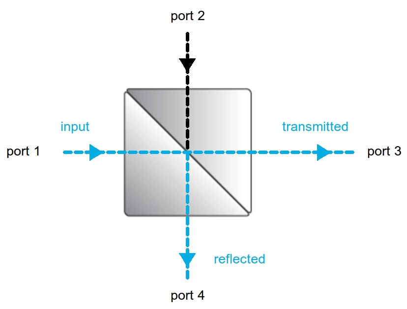
Figure 2.6: Beam Splitter

Polarizing Beamsplitter:
A polarizing beamsplitter is a device that selectively reflects or transmits photons depending on their polarization (the orientation of its electric field). For example, light with polarization V being reflected and H being transmitted. This type of beamsplitter is generally constructed from anisotropic crystals. Light passing through anisotropic (non-uniform) crystals will refract at different angles and spatially separate depending on the light polarization. By choosing the appropriate crystals and angles of incidence, light with one polarization (e.g., vertical) can be completely reflected, while opposing polarization (e.g., horizontal) is completely transmitted. Polarizing beamsplitters are thus a key component in performing a photon polarization measurement. One can infer the photon polarization with a photon detector at each output by measuring a detection event in either the transmission arm or the reflection arm.

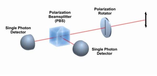
Figure 2.7: Polarized Beam Splitter

Spatial Beamsplitter:
A spatial beamsplitter takes an incoming photon field and transmits it to the output port with a probability T, and reflects it with a probability R. When T=R=50%, we call this a “50:50 beamsplitter.” A spatial beamsplitter is generally described by a 2x2 matrix $U_{\textrm{BS}}$ that takes incoming photon-field amplitudes (we will call them $a_{1}$ and$a_{2}$for short) and outputs transmitted and reflected fields ($a_{3}$ and $a_{4}$).

$$\left(\begin{array}[]{cc}a_{3}\\ a_{4}\end{array}\right)\displaystyle=\displaystyle U_{\textrm{BS}}\left(\begin{array}[]{cc}a_{1}\\ a_{2}\end{array}\right)$$ (2.64)

$$=\displaystyle\left(\begin{array}[]{cc}t&r\\ r&t\end{array}\right)\left(\begin{array}[]{cc}a_{1}\\ a_{2}\end{array}\right)$$ (2.65)

$$\rightarrow a_{3}=ta_{1}+ra_{2}\leavevmode\nobreak\ \leavevmode\nobreak\ \&\leavevmode\nobreak\ \leavevmode\nobreak\ a_{4}=ra_{1}+ta_{2}$$ (2.66)

Since the fields $a_{i}$are amplitudes, it follows that obtaining the photon field energy or photon number requires taking the magnitude squared $|a_{i}|^{2}=a_{i}^{*}a_{i}.$ In cases where these are quantum-mechanical photon-field operators, one similarly calculates an ensemble average $\langle a_{i}^{\dagger}a_{i}\rangle$. The matrix unitarity condition $U_{\textrm{BS}}^{\dagger}U_{\textrm{BS}}=I$ requires that $|r|^{2}+|t|^{2}=1$ and $r^{*}t+t^{*}r=0$, and this ensures that photons are neither lost nor gained in the beamsplitting process. In other words, it conserves probability T+R=1 where $T=|t|^{2}$is the transmission probability and $R=|r|^{2}$ is the reflection probability. For a 50:50 beamsplitter, one can take $r=i/\sqrt{2}$and $t=1/\sqrt{2}$. With this matrix relation in hand, one can calculate the average output field intensity and the intensity fluctuations induced due to the beamsplitter partitioning process.

1. Beam Splitters; When a single photon enters an ideal, lossless 50:50 spatial beam splitter at port 1 shown in Fig. 1, it is partially transmitted to port 3 and partially reflected port 4. Therefore, a single photon leaves the beamsplitter in a superposition state of being in both the transmission and reflection arms. A detection event then randomly collapses the photon into one of those arms, with a 50% chance of detecting the photon in the transmission arm, and a 50% chance of detecting it in the reflection arm. On the other hand, if the beam splitter is a polarizing beam splitter illustrated in Fig. 2, then the horizontal component of the photon is transmitted and detected at port 3, whereas the vertical component gets reflected and detected at port 4. Which of the following phrases is valid?

   

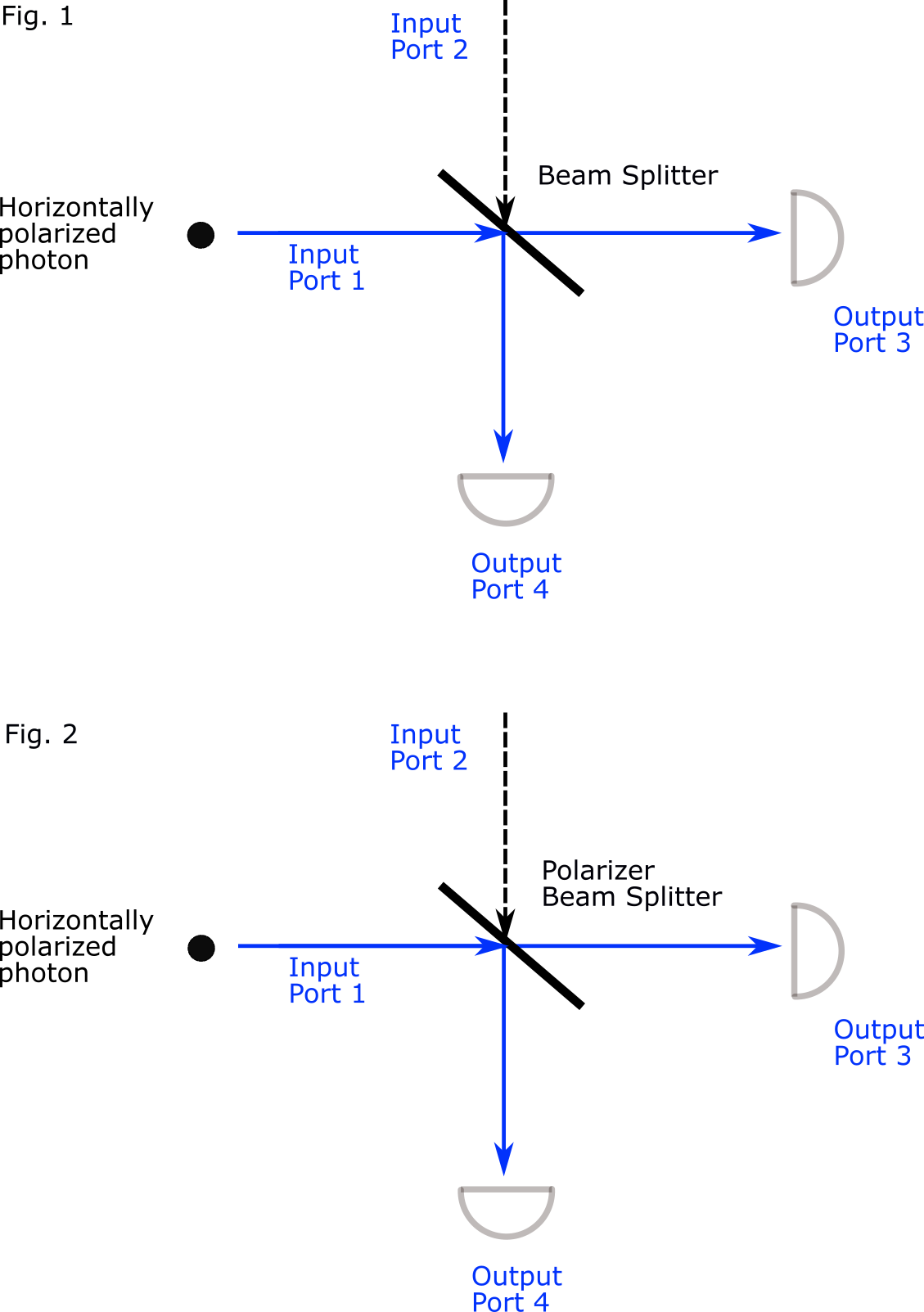
   Figure 2.8: Beam Splitters

   2.23   Quantum Key Distribution - BB84

   Ordinary classical information everybody understands that because it surrounds us. It is like the information in a book. we can copy it at will, and it is not disturbed by reading it. However, what is quantum information[1, 72, 73]? Rather than give a mathematical description, we try to find a metaphor for it. It is rather like the information in a dream. If we try to describe our dream to someone, our memory of it changes, and eventually, we forget the dream, and we only remember what we said about it. we cannot prove to someone else what we dreamed, and we can lie about our dream without getting caught. However, there is no really hard science of dreams, despite the effort of Sigmund Freud. unlike dreams, there is a good mathematical theory of quantum information. Indeed, when we develop it, we will see where classical information comes from, that we used to think was just simple information. well, here are some examples of elementary quantum behavior. we can use single photons of light to carry one bit of information because a horizontal photon, as at the top of the figure, can be reliably distinguished from the vertical photon, as in the middle. if we pass them through a calcite crystal like that, or crystal of any other sufficiently un-symmetric material, the horizontal photons will get passed straight through, and the vertical ones will get deviated by some amount. therefore, we can count them in two separate detectors. that means each photon can carry one reliable bit of classical information. However, if we put in photons at some other angle, instead of being deviated by an intermediate amount, as we might expect, they behave probabilistically. Some go into the upper beam and become horizontal, and the others go into the lower beam and become vertical. It is, we might say, one of the central mysteries of quantum mechanics, the random behavior of things that are individually identically prepared. We can use vertical and horizontal photons to send one bit per photon of the message. However, if we put in diagonal photons, well, simply by rotating the apparatus, we can distinguish a left diagonal from a right diagonal, like a slash from a backslash. However, once that rotated apparatus is used, that thing cannot distinguish the vertical from the horizontal. So, we have four separate states of the photons that are pairwise, perfectly distinguishable. Nevertheless, we cannot distinguish all four kinds. Now we want to get us to worry a little bit about this strange behavior. Bill Wootters, a physics professor, has a pedagogic analog for quantum systems’ behavior when measured. He says it is really like one of those old fashioned 19th-century British schools where the students, who are not supposed to ask any questions they were just supposed to respond to the questions the teacher posed, and where the student is the photon, and the teacher is the measuring apparatus. So, the strict teacher is asking the student a question, saying, is our polarization vertical or horizontal? Furthermore, the students start saying, and we polarized about 56, 55 degrees. we believe we asked a question. Are we vertical or horizontal? Oh, horizontal. Did we ever have any other polarization? No, we were always horizontal. So, that is how quantum systems behave when measured, and that is what lies behind many of the interesting things we can do with it. ultimately, when we come to entanglement, we can understand where that behavior comes from. well, now, we will discuss how we put it to use. This is the quantum money that was proposed by Wiesner in 1968. He says a piece of quantum money will have a serial number on it like ordinary money, but it also will have 20 perfectly reflective boxes, each containing a single photon of one of those four states. the bank will have a record based on the serial number of which photon is in which box, which kind of photon, and when we bring the money back to the bank, the bank will open the boxes, one by one, and measure each photon in the way that it would behave reliably, and therefore check that they all agree with what was supposed to be stored there. However, if we do not know What is stored there, we will disturb some of them by measuring them the wrong way, and the chance of passing a fake bill or making a copy that passes is 3/4 to the 20th power, which is small. It is the idea that Gilles Brassard and Peter Shor used in building the quantum cryptography apparatus where we do not try to store the photons, but we send them over a short distance, which in this case was only about 30 centimeters. the idea is that any eavesdropper in that empty middle section of the apparatus would spoil the sum of the transmitted photons by measuring the wrong way, and therefore, would betray their presence. So, in more detail, the way quantum key distribution works are that we have two parties. we call them Alice and Bob. Alice sends a stream of polar ice photons of those four kinds to Bob. Eve is the nickname for the eavesdropper. She can try to measure those photons if she wants, but if she does, she will introduce errors with high probability. the other thing we allow her to do is to listen to the classical discussion between Alice and Bob. that takes place through a series of ordinary classical messages exchanged over a public channel. when they are done with all this, they end up each with a shared secret key, in other words, a random string that they both know, and they have high confidence that no one else knows. well, that is the case if there is not too much eavesdropping, or there is no eavesdropping, but if there is much eavesdropping, they will detect a lot of errors and effort to distill this key will have failed. However, they will know that it has failed with high probability. they just try again tomorrow. So, in more detail, here is how the protocol works, which is called BB84, after the names of the author and the year that it came out. Alice, in the first line, sends a random sequence of these four kinds of photons. Bob, on the other side, makes random measurements uncorrelated. He does not know what Alice would send, and he randomly chooses to make a rectilinear measurement that is vertical versus horizontal or diagonal. So, he does, and then in the third line, we get his measurement results. we including the realistic effect that some of the photons may get lost or his detectors may not be perfectly efficient. So, in some cases, he does not get anything. For example, in the first case, Alice sent a vertical photon. He chose to make a rectilinear measurement, and he gets a vertical result, which is correct. In the second case, Alice sent a horizontal photon, but he decided to make a diagonal measurement, and he gets a random one of the two diagonal results. However, he does not know that it is bad. It is a 45-degree photon, and so, on for the others. The next stage of the protocol now is, after he is received them, Bob tells Alice which kind of measurement he did. He said we measured the first one rectilinearly, the second one diagonally, the third and fourth one rectilinearly, the fifth one we did not get, and so on. That is indicated by the classical message in quotation marks. then Alice tells him in which cases he did the right thing. That is, he made a measurement that did not spoil the polarization that she sent. She very carefully does not say whether she said vertical or horizontal, but she says in the first case, we made a rectilinear measurement, which was good. Keep that photon. Do not tell what it was, because somebody might be listening. In the second case, too bad, we made a diagonal measurement. we sent a rectilinear photon, and so, on. So, they cull from the photons that Bob received, the ones that he spoiled. we can identify, say, a vertical photon is a 1, a horizontal is 0, or for the diagonal photons, they choose to identify the 45 degrees as a 0, and the 135 is a 1. So, what they have, essentially, at this stage is a bunch of bit values that they ought to agree about if there has been no eavesdropping. So, the next question is to find out whether there has been eavesdropping, and we can do those various ways, but the most economical way that does not involve giving away a lot of the data is for Alice to choose a random subset of the bit positions, and announce the parity of that random subset. in the first case, she chose this collection outlined in red, and it has odd parity. She says that it is odd. then the second one, she chooses a different random subset and says that is even, and they go on for 20 of these random subsets. if they agree about all of them, then the chance that there is even one mistake in their sequence is about one in a million. So, they are pretty happy with that. they have to throw away some of the photons to compensate for the fact that they have leaked 20 bits of information to the eavesdropper. So, that is the elementary version of the BB84 protocol.

   Quantum key distribution (QKD) is a protocol used to distribute shared secret keys with security guarantees that are ideally based on the properties of quantum mechanics, rather than on the presumed computational resources of an eavesdropper. This may be contrasted with classical methods of key exchange, such as the RSA cryptosystem, where security is based on the presumed classical computing complexity of the order-finding problem.

   The first QKD protocol, now commonly referred to as BB84, was introduced in 1984 by Charles H. Bennett from IBM and Gilles Brassard from the University of Montreal. Since then, there have been several proposed QKD protocols, many of which have been demonstrated, including long-range experimental demonstrations via satellite and even commercially available QKD systems.

   The BB84 protocol can be used by a sender (Alice) and a receiver (Bob) who wish to create a shared secret key. It requires that Alice and Bob have access to a quantum channel [79]over which Alice will send polarized photons to Bob and a classical, broadcast channel for coordination purposes. By a broadcast channel, we mean that an eavesdropper (Eve) can listen to and record all information sent over this channel, but she cannot alter it.

   To begin the protocol, Alice produces, records, and sends Bob single photons with polarization encodings each chosen at random from one of the four polarization states:
   

   $\displaystyle|\psi_{H}\rangle\displaystyle=|H\rangle,$

   $\displaystyle|\psi_{V}\rangle\displaystyle=|V\rangle,$

   $\displaystyle|\psi_{+}\rangle\displaystyle=\frac{1}{\sqrt{2}}(|H\rangle+|V\rangle),$

   $\displaystyle|\psi_{-}\rangle\displaystyle=\frac{1}{\sqrt{2}}(|H\rangle-|V\rangle).$

   The first pair and the second pair of states are orthogonal $\langle\psi_{H}|\psi_{V}\rangle=0$ and $\langle\psi_{+}|\psi_{-}\rangle=0$ and, therefore, each pair forms a polarization measurement basis. As such, we can think of photon polarization states as qubit states, with the photon polarization being either in states H and V or in states + and -. Importantly, note that while the states within a basis are orthogonal, states between the two bases are not orthogonal with one another, for example, $\langle\psi_{H}|\psi_{+}\rangle\neq 0.$

   Next, Bob measures each photon in one of the two bases either { H, V} or { +,-} which he chooses at random for each photon, and records the measurement results. Once complete, Bob announces the basis he used for each measurement, but not the result, over the broadcast channel. Because Alice and Bob independently chose the polarization basis at random for each photon, there is a 50-50 chance that they chose the same one for any given photon. For each photon where they did choose the same basis, Alice and Bob will have recorded the same polarization value, because the states within each basis are orthogonal, and we assume an ideal measurement.

   For example, if Alice sends $|\psi_{H}\rangle$ and Bob measures in the $\{H,V\}$ basis, then Bob will also measure and record an H, assuming perfect measurement, since $\langle\psi_{H}|\psi_{H}\rangle=1$ and $\langle\psi_{H}|\psi_{V}\rangle=0$. It is considered a successful trial because both Alice and Bob recorded an H for this photon. However, for the other half of the photons, where Alice and Bob did not select the same basis, the results are uncorrelated, because the two bases are maximally conjugate. It means that a measurement in the wrong basis is equally likely to result in either of the two incorrect outcomes, for example, $|\langle\psi_{H,V}|\psi_{+,-}\rangle|^{2}=\frac{1}{2}.$ It would be considered an unsuccessful trial.

   The security of BB84 starts with the fact that Eve gains no information from listening to the broadcast channel since only information about bases is available and not the measurement results. Thus, she must try to gain information from the photons in the quantum channel [206]. However, any attempt by Eve to extract information reveals her presence through the introduction of abnormalities in the statistics of Bob’s measured results. As a result, Eve is unable to extract information encoded by Alice without alerting Alice and Bob that she is trying to do so.

   A straightforward strategy Eve could use is to intercept each photon and measure it on some basis, record the result, and then send a photon to Bob based on her measurement outcome. In doing this, Eve destroys Alice’s original photon, and due to the no-cloning theorem, Eve cannot precisely reproduce each of Alice’s photons. If Eve got lucky and selected the same polarization basis as Alice did, then she, by chance, will send Bob a photon with the same polarization. However, when Eve does not choose the same basis as Alice, Eve obtains the wrong measurement result, infers a different polarization (without knowing it), and thus sends Bob a photon with a polarization different than Alice’s original photon. Consequently, the statistics of Alice and Bob’s measured results successful trials versus unsuccessful trials and their statistics will be altered by Eve’s activities and reveal her presence.

   Realistically Alice and Bob do not want to throw out the entire key every time an anomaly occurs since even without an eavesdropper, noise and imperfect measurement will always lead to some level of errors and statistical variation. Alice and Bob adopt a strategy called privacy amplification to deal with this problem, which produces a new, shorter, shared key from the original one, which can, in principle, reduce Eve’s inferred information to zero.

   Before implementing privacy amplification, Alice and Bob must first ensure their keys match. They can do this using classical error correction methods: having Alice randomly choose two bits from her key, adding them together modulo 2, and announcing the result to Bob. He, in turn, tries the same and replies with his result. If they match, the two bits are kept. If they differ, the two bits are discarded. Just sending the result of modular addition over the classical channel does not reveal any information to Eve since it only indicates the parity of the bits, that is, whether the two bits have the same or different values, but not their specific values. Using this technique, Alice and Bob will arrive at two matching keys. However, Eve may still have knowledge of a few of these bits (but, certainly not all of them).

   Next, the privacy amplification protocol is applied. Privacy amplification comprises a series of transformations on Alice and Bob’s matching key to create a shorter key, one which Eve cannot replicate without knowing the entire initial key. For example, Alice and Bob jointly choose pairs of bits at random from their keys and replace them with their binary addition. Intuitively, this works because of parity; Eve cannot know the value of the binary addition without knowing the value of both initial bits. Based on the error rates found in Alice and Bob’s initial keys, they can estimate how much information Eve has and then reduce it to the desired level (approaching zero) using the privacy amplification protocol.

   So far, we have only dealt with eavesdropping in the ideal case; however, real-world implementations of BB84 and other QKD protocols are potentially open to a much wider range of system-level vulnerabilities. For example, if attenuated classical light is used to generate single photons rather than a true single-photon source, photon number splitting attacks become possible on residual states with more than one photon. In this case, Eve can split off and measure one of the photons in the multi-photon state without impacting the polarization that reaches Bob. Besides, access to the hardware at Alice and Bob’s locations must be restricted to trusted personnel only. Otherwise, an Eavesdropper can gain access to the random number generator used to select bases or even the encoded keys themselves by other means. There are just a few examples of the types of attacks, many of which are independent of the quantum nature of QKD that may compromise the quantum-enhanced security afforded by an ideally implemented QKD system.

   So, the Chinese satellite perform QKD [26], used to perform quantum cryptography, and the secure communication, and, how does this work, That satellite is independently communicating with two points on the ground. so, it is the satellite that is doing the exclusive or of the message with the pads, then independently, when it is over one city, it is communicating with that city, and then it carries the information when it is on the other side of the earth, communicating with another city. it is then also communicating with that side. so, the satellite is acting basically as a relay, and performing the quantum cryptography during that transit.

   2.24   Entangled Photon Sources and Detectors

   So, for this section, we have introduced single-photon sources and detectors and seen how single photons can be used to encode and transfer quantum information across a communication channel, for example, to distribute a cryptographic key. In this section, we will discuss the generation in the detection of entangled pairs of photons. later this section, we will discuss how entangled photons may also be used for quantum key distribution, as well as for quantum teleportation and random number generation[204]. As discussed in section 1, an entangled state is a manifestly quantum mechanical multi-qubit state that cannot be written as a product of single-qubit states. Let us start with a counter-example. we have seen through section 1 and section 2 that if we apply Hadamard gates to 2 qubits, each prepared in state zero, then we obtain the 2 qubits equal superposition state, 0, 0 plus 0, 1 plus 1, 0, plus 1, 1. While it might appear that this state cannot be factored into single-qubit states, we know it is possible because we generated it by applying Hadamards to single qubits. as we have seen, this state is the tensor product [78, 85] of the single-qubit superposition state 0 plus 1. Thus, it is not an entangled state, because we can write it in terms of the single-qubit states ; 0 plus 1 for qubit A, tensor product 0 plus 1 for qubit B. In fact, 0 plus or minus 1 are the excited and ground states along the x-axis of the block sphere. Thus, we can write this as the plus and minus state in the x spaces. In contrast, we can see that state 0, 0 plus 1, 1 cannot be written as a tensor product of single-qubit states. it is an entangled state of 2 qubits called a Bell state. even when we perform a transformation to the x basis, we still get a state that cannot be factored into single-qubit states A, tensor product B. This is a property of entangled states. They remain untangled even on different bases. looking at the circuit model, we see that we needed a conditional 2 qubit gate to generate the entanglement. Single qubit gates alone were not enough. we will return to Bell states in a moment. Recall from earlier this section that single photons have a polarization, for example, horizontal and vertical. since vertical and horizontal polarizations are orthogonal quantum states, we choose to put them at the poles of the block sphere and call this the qubit. For single-photon QKD protocols, like BB84, this is sufficient. Bob preparers a single photon in a particular qubit state that is a particular polarization state and then sends it along the communication channel to Alice. However, as we will see in the next couple of sections, using entangled photons enables certain alternative types of QKD protocols, as well as a means to generate random numbers in teleport quantum information. Thus, the question is, how do we generate and detect entangled photons? The most common method for producing entangled photons is through a process called spontaneous parametric downconversion. Parametric downconversion is essentially a frequency conversion process, where a photon at frequency 2f is converted into two individual photons whose frequencies together add to 2f and conserve energy, for example, each photon having a frequency, f. Now, linear time-invariant systems, by definition, do not convert frequencies. If we take a sine wave and pass it through a linear system, its amplitude and phase may change, but its frequency remains the same. It is essentially a statement that a plane wave e to the i omega t is an eigenfunction of a linear system. Thus, to take a photon at one frequency and convert into two photons at a different frequency, we need a material with strong nonlinear optical properties. a common example of such a crystal is beta barium borate or BBO. When a strong pump beam passes through a BBO crystal, there is a small probability that one of its photons will convert into two photons, one called a signal, and the other called an idler. It is just convention. Now, due to energy conservation, the signal and idler frequencies are each half of the pump frequency. due to momentum conservation, the signal and idler photons will leave the crystal in correlated spatial directions. Additionally, these two photons will also have correlated polarizations. Depending on the type of crystal we use. The two downconverted photons will either have the same polarization, which we call a Type 1 Crystal, or they have opposite polarizations from a type 2 Crystal. BBO is a Type 2 Crystal. We see that the two downconverted photons exit the crystal in directions that form a cone, one having horizontal polarization and one having vertical polarization. The locations of the photons on the cones are correlated, equidistant from the original beam trajectory, again, due to momentum conservation. For example, the colored dots on the polarization cones indicate the correlated spatial positions of the emitted photons. Now, crucially for the two photons to be polarization entangled, their direction of emission cannot indicate which photon is vertically polarized and which is horizontally polarized. Therefore, we use an iris to selectively keep only photons that arise from positions where the two polarization cones cross. Thus, whether the signal and idler photons travel left or right once they exit the crystal, one will have polarization h and the other polarization v. Nevertheless, which is not known. In other words, the direction of propagation does not label the polarization. Under these conditions, the state of the two downconverted photons is polarization-entangled, and it is all of the form H, V plus e to i $\phi$ V, H. The phase $\phi$ can be made 0 degrees by choosing the correct phase-matching conditions, crystal thickness, or using a phase shifter. Thus, one has the state H, V plus V, H. This is one of the four Bell states. from this, the other Bell states can be generated by changing the phase $\phi$ and swapping the polarizations H and V, using a half-wave plate. Now that we are able to generate all four entangled Bell states Let us see how to detect these states. we first need to introduce an optical device called a polarization beam splitter [143]. A polarization beam splitter will transmit or reflect a photon depending on its polarization, H or V. at each output of the beam splitter is a single-photon detector. By seeing which detector clicks, we can determine whether the photon had horizontal or vertical polarization. To see how this works, let us try a test case. we begin with a photon polarized in the vertical direction. we also show here for completeness a polarization rotator, a device that changes the polarization of incoming photons. For now, however, we just set it so that it passes photons without making any changes. If we send in a vertically polarized photon, it reflects off the polarization beam splitter, which is detected by the single-photon detector in the reflection arm. On the other hand, if we send in a horizontally polarized photon, it is transmitted by the polarization beam splitter and detected using the single-photon detector in the transmission arm. Thus, we can determine the photon polarization by seeing which detector clicks. So, what happens if we have entangled photons? Let us take the H, V plus V, H entangled state. Photon A travels to the left polarization beam splitter, and Photon B travels to the right polarization being splitter. what we will observe are correlated detection events. That is, if Photon A’s polarization analyzer indicates horizontal polarization, then the Photon B analyzer indicates vertical polarization. Similarly, if Photon A is measured to have a vertical polarization, then Photon B must have horizontal polarization. These are correlated detection events. Now, the presence of correlation suggests polarization entanglement, but it is not proof of entanglement. After all, the source may randomly send out classical states of either H, V, or V, H, which would give the same results. However, it is not an entangled quantum state H, V plus V, H. To test for entanglement, one needs to measure the entanglement in different polarization bases[137]. As we discussed earlier, changing the bases does not change the entanglement. Thus, the measured correlations will be retained in any measurement basis. In practice, rather than changing the measurement hardware, one may instead rotate the input state’s polarization. This is experimentally more straightforward, and this is the role of the polarization rotator. With correlation measurements made on different polarization bases, one can compare the measured results with the classical probability model, assuming there is no entanglement. This type of test is called Bell’s inequality test. it is used to determine the degree of entanglement of a quantum state within certain assumptions, called loopholes. we will discuss more Bell state measurements, test the Bell’s inequality and loopholes later in the section, as well as the application of Bell state measurements to the problem of random number generation.

   Entanglement is a manifestly quantum mechanical state of two or more quantum systems whereby the state as a whole cannot be reduced to a representation of independent, single-system states[168]. For example, the two-qubit state $|\Psi\rangle_{12}=\frac{1}{\sqrt{2}}(|0\rangle_{1}|1\rangle_{2}+|1\rangle_{1}|0\rangle_{2}),$ cannot be written as a tensor product of two single-qubit states $|\phi\rangle_{1}\otimes|\psi\rangle_{2}.$ Moreover, we will find that we always get terms that do not appear in $|\Psi\rangle$. The entanglement of two quantum mechanical two-level systems results in what is referred to as Bell states, and there are various means to generate and detect the kinds of quantum states. However, they all share certain features, as we describe below, including the need for some type of two-body “nonlinearity” to generate and detect these states, whether a nonlinear crystal, a controlled-NOT gate, photon-number resolving detectors that distinguish 0, 1, and 2 photons.

   In the case of photons, a common approach to generated Bell states is spontaneous parametric downconversion (SPDC), as described in the section. In this case, a nonlinear crystal, such as one made from beta-barium borate (BBO), converts incident “pump” photons at frequency $\omega_{p}$ into two photons: a signal photon at frequency $\omega_{s}$ and an idler photon at frequency $\omega_{i}$. The process is energy conserving, and hence the frequencies of the two newly created photons will sum to that of the original pump photon: $\omega_{p}=\omega_{s}+\omega_{i}$ (Planck-Einstein relation). Similarly, the process is momentum conserving, and the vector momenta similar sum together as $\vec{k_{p}}=\vec{k_{s}}+\vec{k_{i}}.$ Since the momenta $\vec{k_{s}}$ and $\vec{k_{i}}$ are vector quantities, momentum conservation correlates both the magnitude of the momentum and the directionality of the emitted photons.

   

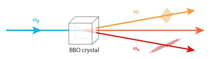
   Figure 2.9: Spontaneous Parametric Down conversion

   There are two general types of SPDC. Type-I SPDC generates two photons with the same polarization, and Type-II SPDC will generate two photons with orthogonal polarization. In both cases, the photons are correlated and, in certain instances, polarization-entangled. As we discuss in the section, BBO is a Type-II SPDC crystal, and so its output comprises a horizontally (H) and a vertically (V) polarized photon. The photon emission forms two cones, one for each polarization. The locations of any two down-converted photons on their respective cones are correlated due to momentum conservation. Thus, in general, the direction of the emission “labels” the photon polarization, such that the resulting two-photon state is not polarization-entangled. However, by selecting photon emission only from the two locations where the two cones cross, the emission direction no longer uniquely specifies the polarization and, in this case, a polarization-entangled state is formed of the form $|\Psi\rangle=\frac{1}{\sqrt{2}}(|H\rangle_{s}|V\rangle_{i}+e^{i\phi}|V\rangle_{s}|H\rangle_{i})$. By choosing the correct phase-matching conditions (e.g., size of the crystal, etc.), one can set the value of $\phi$ and generate the state $|\Psi^{-}\rangle=\frac{1}{\sqrt{2}}(|H\rangle_{s}|V\rangle_{i}-|V\rangle_{s}|H\rangle_{i})$. In the following section, we will look at how to generate the three other Bell states starting from $|\Psi^{-}\rangle.$

   

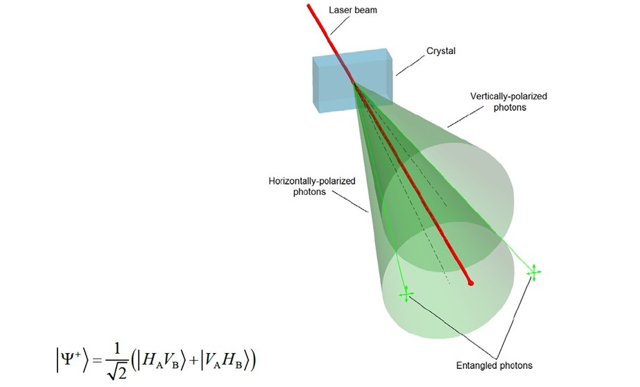
   Figure 2.10: Spontaneous Parametric Down conversion

   Generating the Four Bell States:
   In general, it is possible to create all four Bell states, given just one of them. For a polarization-entangled Bell state with horizontal and vertical polarization, this can be accomplished using optical elements called “waveplates.” Waveplates rotate the polarization axis around the direction of propagation by a specific angle chosen by the design of the waveplate. The waveplate material a birefringent crystal such as quartz has polarization-dependent refractive indices which enable a particular polarization to propagate faster through the material the “fast axis” than the polarization orthogonal to it the “slow axis.” These two axes form a two-dimensional coordinate system.

   Suppose a linearly polarized photon is incident on a waveplate. The overall phase accumulated while the photon travels through the waveplate depends on the waveplate thickness corresponding to the distance the photon has to propagate to pass through the optical element. However, in addition, the photon polarization is projected on to the waveplate’s coordinate system, and the portion along the slow axis accumulates an additional phase with respect to the component along the fast axis.

   If the “extra” phase is equivalent to one-half the incident photon wavelength, the waveplate is referred to as a “half-wave plate.” Moreover, the angle between the half-wave plate coordinate system relative to the photon’s polarization axis determines the projections onto the fast and slow axes and, thus, the rotation of the polarization.

   With two half-wave plates, it is possible to generate all Bell states starting from one of them. Two transformations need to occur: 1) a polarization change that swaps $|H\rangle$ and$|V\rangle,$ and 2) a phase shift $\phi=\pi$ that swaps + and -. To swap polarization, the half-wave plate’s coordinate system is oriented $45^{\circ}$ with respect to the photon polarization axis. To impart a phase shift, another half-wave plate’s fast axis can be oriented $-45^{\circ}$ with respect to the horizontal axis to induce a phase inversion.

   The following table summarizes the required optical elements a polarization swapping half-wave plate, $HWP_{45^{\circ}},$and a phase inversion half-wave plate, $HWP_{0^{\circ}}-$ to alter the polarization of the first photon $p_{1}$ or the second photon $p_{2}$ and what general quantum gate that corresponds to to generate all four Bell states starting with $|\Psi^{+}\rangle=\frac{1}{\sqrt{2}}(|H\rangle_{1}|V\rangle_{2}+|V\rangle_{1}|H\rangle_{2})=\frac{1}{\sqrt{2}}(|0\rangle_{1}|1\rangle_{2}+|1\rangle_{1}|0\rangle_{2}).$

   Table 2.5: optical elements - a polarization swapping half-wave plate

   Target	p_2: Optical Element	Gate	Polarization	General
   $|\Psi^{+}\rangle$	No elements	$I\otimes I$	$\frac{1}{\sqrt{2}}(|H\rangle_{1}|V\rangle_{2}+|V\rangle_{1}|H\rangle_{2})$	$\frac{1}{\sqrt{2}}(|0\rangle_{1}|1\rangle_{2}+|1\rangle_{1}|0\rangle_{2})$
   $|\Psi^{-}\rangle$	$HWP_{0^{\circ}}$	$I\otimes Z$	$\frac{1}{\sqrt{2}}(|H\rangle_{1}|V\rangle_{2}-|V\rangle_{1}|H\rangle_{2})$	$\frac{1}{\sqrt{2}}(|0\rangle_{1}|1\rangle_{2}-|1\rangle_{1}|0\rangle_{2})$
   $|\Phi^{+}\rangle$	$HWP_{45^{\circ}}$	$I\otimes X$	$\frac{1}{\sqrt{2}}(|H\rangle_{1}|H\rangle_{2}+|V\rangle_{1}|V\rangle_{2})$	$\frac{1}{\sqrt{2}}(|0\rangle_{1}|0\rangle_{2}+|1\rangle_{1}|1\rangle_{2})$
   $|\Phi^{-}\rangle$	$HWP_{0^{\circ}},HWP_{45^{\circ}}$	$I\otimes ZX$	$\frac{1}{\sqrt{2}}(|H\rangle_{1}|H\rangle_{2}-|V\rangle_{1}|V\rangle_{2})$	$\frac{1}{\sqrt{2}}(|0\rangle_{1}|0\rangle_{2}-|1\rangle_{1}|1\rangle_{2})$

   Detection of Bell States:
   To determine the success of the generation of a particular type of Bell state, detection schemes that distinguish all four Bell states are necessary. A deterministic measurement of Bell states generally requires nonlinear elements and two-particle interactions capable of performing conditional two-qubit rotations, two-particle interferometry (e.g., Hong-Ou-Mandel experiment sensitive to quantum statistics), number-resolving photodetectors, and the like. The details and trade-space of the various types of Bell state analyzers are beyond the scope of this text unit. For our purposes here, we will consider one example of a Bell-state analysis which uses the CNOT gate as the conditional[136], two-qubit gate and apply it to our photon polarization-entangled Bell-state example.

   Since photons interact only weakly (if at all), it is challenging to make reliable, nonlinear optical elements that implement deterministic, nonlinear operations with high efficiency. Linear optical elements are reliable, but they cannot be used to distinguish all four polarization-entangled Bell states deterministically. However, there are probabilistic schemes that can distinguish the Bell states using linear optics. In this case, one must identically prepare the same Bell state many times and run protocols using linear optical elements followed by measurement. Through these schemes, effective nonlinear interactions can be realized probabilistically and detected through an appropriate measurement scheme. When a spectator measurement indicates that an effective interaction has occurred, the results from that specific experimental trial are kept and aggregated to perform the Bell-state analysis; this is called post-selection. For example, although there is no deterministic CNOT gate with solely linear optics, there is a scheme for implementing a probabilistic, CNOT gate with linear optics that can be leveraged with measurement post-selection.

   The following general protocol is able to distinguish all four Bell states. It can be implemented in a probabilistic manner with a probabilistic CNOT gate following Emanuel Knill’s, Raymond Laflamme’s, and Gerard Milburn’s proposal and a beamsplitter as a Hadamard gate. Note that in the notation below, we use $|0\rangle$ and $|1\rangle$ to represent the polarization states $|H\rangle$and $|V\rangle,$ so as not to confound the polarization state $|H\rangle$ with the Hadamard gate H .
   $\displaystyle|\Psi^{+}\rangle=\frac{1}{\sqrt{2}}(|0\rangle_{1}|1\rangle_{2}+|1\rangle_{1}|0\rangle_{2})\xrightarrow{CNOT}$ $\displaystyle\frac{1}{\sqrt{2}}(|0\rangle_{1}|1\rangle_{2}+|1\rangle_{1}|1\rangle_{2})\xrightarrow{\leavevmode\nobreak\ H\otimes I\leavevmode\nobreak\ }\displaystyle|0\rangle_{1}|1\rangle_{2}$
   $\displaystyle|\Psi^{-}\rangle=\frac{1}{\sqrt{2}}(|0\rangle_{1}|1\rangle_{2}-|1\rangle_{1}|0\rangle_{2})\xrightarrow{CNOT}$ $\displaystyle\frac{1}{\sqrt{2}}(|0\rangle_{1}|1\rangle_{2}-|1\rangle_{1}|1\rangle_{2})\xrightarrow{\leavevmode\nobreak\ H\otimes I\leavevmode\nobreak\ }\displaystyle|1\rangle_{1}|1\rangle_{2}$
   

   $\displaystyle|\Phi^{+}\rangle=\frac{1}{\sqrt{2}}(|0\rangle_{1}|0\rangle_{2}+|1\rangle_{1}|1\rangle_{2})\xrightarrow{CNOT}\displaystyle\frac{1}{\sqrt{2}}(|0\rangle_{1}|0\rangle_{2}+|1\rangle_{1}|0\rangle_{2})\xrightarrow{\leavevmode\nobreak\ H\otimes I\leavevmode\nobreak\ }\displaystyle|0\rangle_{1}|0\rangle_{2}$
   

   $\displaystyle|\Phi^{-}\rangle=\frac{1}{\sqrt{2}}(|0\rangle_{1}|0\rangle_{2}-|1\rangle_{1}|1\rangle_{2})\xrightarrow{CNOT}\displaystyle\frac{1}{\sqrt{2}}(|0\rangle_{1}|0\rangle_{2}-|1\rangle_{1}|0\rangle_{2})\xrightarrow{\leavevmode\nobreak\ H\otimes I\leavevmode\nobreak\ }\displaystyle|1\rangle_{1}|0\rangle_{2}$
   

   The two-qubit states are measured after a CNOT gate, and the Hadamard gate on the first qubit is applied. The measurement reveals the underlying type of the Bell state.

   2.25   Quantum Key Distribution - Ekert91 and BBM92

   There are various forms of quantum key distribution or QKD described by different protocols. They all make use of quantum mechanical properties to establish shared lists of random numbers that can be used for encryption. we have discussed the BB84 QKD protocol where one user, Alice, prepares a specific state that she sends to another user, Bob. Bob then measures the state. Alice and Bob then perform sifting by comparing the preparation basis and the measurement basis and then following several classical postprocessing steps to establish secure encryption keys. Protocols of this sort, which make use of quantum superposition where one party prepares a state and the other party measures it, are called to prepare and measure QKD protocols. An alternative set of protocols is called entanglement-based protocols, and they make use of entanglement. Two common and related entanglement-based protocols are the BBM92 protocol, named for its inventors Bennett, Brassard, and Merman. Its invention, the year of 1992, and E91 or Ekert protocol, was invented by Artur Ekert in 1991. In both of these protocols, a transmitter consisting of an entanglement source generates a two-photon entangled state known as a maximally entangled Bell state, with one photon being sent to Alice and the other photon being sent to Bob. The photons are sent across quantum communication channels that can reliably transmit the single-photon states and preserve their entanglement. The relevant property of Bell states is that the photons are correlated in multiple measurement bases, including the basis consisting of the horizontal and vertical photon polarizations and the 45-degree rotated basis consisting of the diagonal and the antidiagonal polarizations. For an ideal transmission across the channel, if Alice and Bob choose the same measurement basis, their measurement results will be perfectly correlated between the measurement devices. However, individual measurements at each side will look random. Alternately, if Alice chooses the horizontal-vertical basis and Bob chooses the diagonal-antidiagonal measurement basis, the measurements will not be correlated at all. for intermediate basis choices, their measurements will be partly correlated. In the BBM92 protocol, Alice and Bob received their entangled photon, and both choose either the horizontal-vertical or the diagonal-antidiagonal measurement basis. They both record their basis choice and what the actual measurement result is. They repeat this many times, and they now have long lists of chosen measurement bases and measurement results. The remaining protocol steps are identical to the previously described BB84 protocol; namely, Alice and Bob use a classical communication channel to announce their chosen measurement bases to sift out only the instances of them choosing the same basis. They then compare a random subset of measurement results to determine how well the quantum channel performed. if the determined error rate is below 20%, they perform classical postprocessing to erase any information that a potential eavesdropper could have discovered and correct for remaining errors between Alice and Bob. The benefit of the BBM92 protocol is that the protocol does not require that we trust the source that prepares and sends the state. The protocol ensures that there is no way for a malicious actor to take control of the source and spoof Alice and Bob without them detecting it by observing lower correlation strengths and thus higher error rates than are required to form a secure key. The other entanglement-based protocol, the Ekert protocol, is similar but adds an interesting twist. In this protocol, the same sort of state is generated and distributed between Alice and Bob. Alice randomly chooses between three measurement bases: the horizontal-vertical basis, the 45-degree rotated diagonal-antidiagonal basis, and an intermediate basis rotated by 22 and 1/2 degrees. Bob also randomly chooses between three bases the horizontal-vertical basis, the intermediate 22 and 1/2-degree rotated basis, and a final basis rotated by 67 and 1/2 degrees. The measurement bases and the measurement results are recorded. Alice and Bob repeat this many times and again announce their chosen measurement bases over a public classical communication channel. The instances where they have chosen the same basis are used for the key-generation process. The instances where they have chosen different bases are used to determine the performance of the channel. For these instances, the measurement results are announced publicly and are used in a Bell inequality to determine how well the channel transmission has preserved entanglement. This allows Alice and Bob to have an entanglement-based measurement of the maximum amount of information a potential eavesdropper could have obtained. Alice and Bob then perform classical postprocessing to erase any information an eavesdropper could have discovered and to correct for remaining errors between Alice and Bob. That is how entanglement can establish encryption keys, eliminate the need to trust the system transmitter, and check the security of the encryption keys. There are various other QKD protocols with differing benefits and tradeoffs that may be of interest to specific scenarios. However, the important point is that they all make use of the same basic ideas and concepts that we have described here.

   The first quantum key distribution (QKD) protocol BB84 encoded information in the polarization of single photons. BB84 uses a quantum channel to communicate the photons, and a classical channel to broadcast the chosen polarization bases used for preparation and measurement.

   In this section, we will present an alternative method proposed by Artur Ekert in 1991, known as Ekert91, which encodes information using polarization-entangled Bell states. Ekert91 also uses a quantum and classical channel. However, the advantage of the Ekert91 protocol is that its security can be traced directly to fundamental properties of quantum mechanics entanglement and measurement through a test called Bell’s inequality. In this section, we will discuss Bell’s inequality and its use in Ekert91 to communicate information securely and detect the presence of an eavesdropper.
   Entanglement and Bell’s Inequality:
   In 1935, Albert Einstein, Boris Podolsky, and Nathan Rosen (EPR) argued that quantum mechanics is an incomplete theory in a scientific article titled “Can Quantum-Mechanical Description of Physical Reality Be Considered Complete?.” Their argument was a thought experiment that can be related to two-particle entanglement. Essentially, imagine that we take a polarization-entangled state of two photons, and we then send one photon each to Alice and Bob. A very large distance separates them. If Bob and Alice measure on the same basis, then their results should be correlated, for example, if Bob measures H, then Alice measures V., if they measure on different bases, then their measurements are uncorrelated.

   However, what happens if Alice and Bob are separated by a distance so large that they can make their independent measurements faster than it would take light (and thus information) to travel between their locations? Then, we are left with the conundrum called the EPR paradox. Essentially, due to entanglement, there is a quantum-mechanical correlation in the measurements made by Alice and Bob. It is more than simply “if Alice measures H then Bob measures V.” Bob’s results correlated or uncorrelated depend on Alice’s choice of basis; but, Bob makes his measurement long before any knowledge of Alice’s choice could have reached him or his measurement apparatus. Einstein did not like such “spooky action at a distance,” and thus hypothesized that quantum mechanics theory must be incomplete, that there must be “hidden variables” that quantum theory does not account for to connect these measurements. So the perceived randomness of quantum mechanical measurement is a mirage.

   Niels Bohr, a contemporary of Einstien, responded the same year in a scientific article with the same title and argued that the theory of quantum mechanics only captures the interaction of a quantum system with a measurement apparatus and not the intrinsic character of it. Therefore, any conclusion based on the assumption that measurement does not disturb the measured system in question such as the EPR conjecture that quantum theory is incomplete without hidden variables must be invalid[257].

   The debate continued for decades. In 1964, John Bell proposed a theorem later referred to as Bell’s inequality, which can be used to test if hidden variables do exist experimentally. Essentially, Bell’s inequality is a statement based on purely classical arguments. If the inequality is violated in experimental measurements, quantum mechanics must be complete, and there are no hidden variables. In 1969, John Clauser, Michael Horne, Abner Shimony, and Richard Holt presented a method to quantify Bell’s inequality theorem, abbreviated as the CHSH inequality. If the measurement results of a probed quantum system do not exceed a certain threshold, the CHSH inequality is true and hidden variables do indeed exist. In contrast, if the theorem is violated, thus a value exceeding this particular threshold results, true randomness exists.

   Suppose Alice and Bob have each a photon from the spin-singlet state $|\Psi^{-}\rangle=\frac{1}{\sqrt{2}}(|0\rangle_{A}|1\rangle_{B}-|1\rangle_{A}|0\rangle_{B}).$ Alice randomly chooses between two different options to measure her photon, Q or R, once her photon arrives at her laboratory. Similarly, upon arrival of his photon, Bob randomly decides between two other measurements, S or T. Since Alice and Bob decide on and execute the type of measurement of their photon at the same time, any disturbance of each other’s process can be ruled out, and information can not propagate faster than light. Their measurements yield either 1 or -1. Considering all different measurement outcomes and some potential noise in the process, the following Bell’s inequality with the expectation value $\mathrm{E}(x)$ being the probability-weighted average of all possible measurement outcomes $x\in\{-1,1\}$ is always true if there exist a set of hidden variables.

   $$|\mathrm{E}(QS)+\mathrm{E}(RS)+\mathrm{E}(RT)-\mathrm{E}(QT)|\leq 2$$ (2.67)

   Incorporating the rules of quantum mechanics and the definition of Alice’s and Bob’s measurements as single or combinations of quantum Z-gates and X-gates, Q,R,S, and T can for example be expressed the following way:

   $$\hat{Q}=Z_{1}\leavevmode\nobreak\ ,\leavevmode\nobreak\ \leavevmode\nobreak\ \leavevmode\nobreak\ \leavevmode\nobreak\ \leavevmode\nobreak\ \leavevmode\nobreak\ \leavevmode\nobreak\ \hat{R}=X_{1}\leavevmode\nobreak\ ,\leavevmode\nobreak\ \leavevmode\nobreak\ \leavevmode\nobreak\ \leavevmode\nobreak\ \leavevmode\nobreak\ \leavevmode\nobreak\ \leavevmode\nobreak\ \hat{S}=\frac{-Z_{2}-X_{2}}{\sqrt{2}}\leavevmode\nobreak\ ,\leavevmode\nobreak\ \leavevmode\nobreak\ \leavevmode\nobreak\ \leavevmode\nobreak\ \leavevmode\nobreak\ \leavevmode\nobreak\ \leavevmode\nobreak\ \hat{T}=\frac{Z_{2}-X_{2}}{\sqrt{2}}$$ (2.68)

   The expectation value for $\langle\hat{Q}\hat{S}\rangle$ results to be:

   $$\langle\Psi^{-}|\hat{Q}\hat{S}|\Psi^{-}\rangle\displaystyle=\displaystyle\frac{\langle 0|_{A}\langle 1|_{B}-\langle 1|_{A}\langle 0|_{B}}{\sqrt{2}}\left(Z_{1}\otimes\frac{-Z_{2}-X_{2}}{\sqrt{2}}\right)\frac{|0\rangle_{A}|1\rangle_{B}-|1\rangle_{A}|0\rangle_{B}}{\sqrt{2}}$$ (2.69)

   $$=\displaystyle\frac{\langle 0|_{A}\langle 1|_{B}-\langle 1|_{A}\langle 0|_{B}}{\sqrt{2}}\frac{-|1\rangle_{A}|0\rangle_{B}-|1\rangle_{A}|1\rangle_{B}+|0\rangle_{A}|1\rangle_{B}-|0\rangle_{A}|0\rangle_{B}}{2})$$ (2.70)

   $$=\displaystyle\frac{1}{\sqrt{2}}\frac{1+1}{2}={\frac{1}{\sqrt{2}}}={\langle\hat{Q}\hat{S}\rangle}$$ (2.71)

   Similarly, $\langle\hat{R}\hat{S}\rangle=\frac{1}{\sqrt{2}},\langle\hat{R}\hat{T}\rangle=\frac{1}{\sqrt{2}},$ and $\langle\hat{Q}\hat{T}\rangle=-\frac{1}{\sqrt{2}}$ can be derived. The resulting expectation values following the rules of quantum mechanics violate Bell’s inequality.

   $$\langle\hat{Q}\hat{S}\rangle+\langle\hat{R}\hat{S}\rangle+\langle\hat{R}\hat{T}\rangle-\langle\hat{Q}\hat{T}\rangle=2\sqrt{2}{>2}$$ (2.72)

   The violation of Bell’s inequality is experimentally confirmed ruling out the existence of hidden variables and thus quantum mechanics is complete.
   Ekert91 and BBM92:
   The entangled states can be generated by a trusted source such as Alice or Bob. The required entangled state is the spin singlet state $|\Psi^{-}\rangle=\frac{1}{\sqrt{2}}(|H\rangle_{1}|V\rangle_{2}-|V\rangle_{1}|H\rangle_{2})=\frac{1}{\sqrt{2}}(|0\rangle_{1}|1\rangle_{2}-|1\rangle_{1}|0\rangle_{2}).$ The particles are spatially separated, one is sent to Alice and one to Bob. Both perform measurements on their photon’s polarization along three different unit vectors $\vec{a}_{i}$ and $\vec{b}_{j}$ respectively. Alice measures randomly relative to the horizontal axis along a unit vector $\vec{a}$ with angle $\phi_{1}^{A}=0^{\circ},\phi_{2}^{A}=45^{\circ},$ or $\phi_{3}^{A}=90^{\circ}.$ In contrast, Bob measures randomly along a unit vector $\vec{b}$ with angle $\phi_{1}^{B}=45^{\circ},\phi_{2}^{B}=90^{\circ},or\phi_{3}^{B}=135^{\circ}.$

   Similarly to BB84, upon completion of all measurements, Alice and Bob publicly share along which orientation each photon was measured. The group for which they picked the same measurement procedure $(\vec{a}_{2},\vec{b}_{1})$ $and$ $(\vec{a}_{3},\vec{b}_{2})$ serve as the group which the key can be generated from. The group of measurements with differing measurement orientations $(\vec{a}_{1},\vec{b}_{1}),$ $(\vec{a}_{1},\vec{b}_{2}),(\vec{a}_{1},\vec{b}_{3}),(\vec{a}_{2},\vec{b}_{2}),(\vec{a}_{2},\vec{b}_{3}),(\vec{a}_{3},\vec{b}_{1}),$ and $(\vec{a}_{3},\vec{b}_{3})$ are used to evaluate the existence of potential eavesdroppers. The measurement results of the second group can be revealed publicly to evaluate via the CHSH inequality if the channel is corrupted or not. The CHSH inequality requires the subset $(\vec{a}_{1},\vec{b}_{1}),(\vec{a}_{1},\vec{b}_{3}),(\vec{a}_{3},\vec{b}_{1}),$ and $(\vec{a}_{3},\vec{b}_{3})$ to work and yields $-2\sqrt{2}$if the quantum channel is not corrupted and hence secure.

   $$S=\mathrm{E}(\vec{a}_{1},\vec{b}_{1})-\mathrm{E}(\vec{a}_{1},\vec{b}_{3})+\mathrm{E}(\vec{a}_{3},\vec{b}_{1})+\mathrm{E}(\vec{a}_{3},\vec{b}_{3})=-2\sqrt{2}$$ (2.73)

   The CHSH inequality is true, meaning the absolute value of the result is $|S|\leq 2$ if the quantum channel is intercepted and one or both photons are disturbed and hence lost some aspects of their “quantumness.” Unless the CHSH inequality is true, Alice and Bob can proceed and define an arbitrary subset of the group with the same measurement procedure to serve as a secret key. Ekert91 utilizes the completeness of quantum mechanics to generate a secret key and distinguishes itself from BB84 by the information carrier of choice, entangled spin-singlet states instead of single photons.

   Shortly after, Charles Bennett, Gilles Brassard, and N. David Mermin generalized BB84 and Ekert91, referred to as BBM92. The BBM92 protocol is equivalent to BB84 and a simplified version of Ekert91 that does not require entangled states and Bell’s inequality to ensure its security. It is able to withstand all known attacks allowed by the properties of quantum mechanics.

   2.26   Random Numbers: An Introduction

   we are going to discuss random numbers. This is a fascinating topic because random numbers are not only really useful in everyday life but thinking about random number generators also brings up some interesting questions about reality and free will. Let us start out discussing why random numbers are so important. If we were a kid in the 80s, we might remember a game show called Press our Luck. Part of the game show had a box moving around different squares on a board that was also changing, and the player would press a button to stop the motion of the box. Whatever square the box was on would be what the player would win, or they could land on a whammy and lose everything. In 1984, Michael Larson went on the show, and he did well. We notice that he pays much attention, almost like he knows when to press the button. he did because the people that made this game did a really bad job randomizing the motion of the box and the squares. They were not random at all, but just randomly picked from a small number of possible sequences. So, Michael Larson spent much time with a VCR watching and memorizing the various, quote-unquote, random sequences that would come up. He ended up setting a record by winning over $100,000, which we sure had consequences for the people who ran the game show. So, that is one-way random numbers can influence someone’s life. here is another more serious one. As we know, the security of many forms of encryption relies on the computational difficulty of solving certain problems. For example, factoring is difficult with a classical computer, so some types of encryption are based on factoring’s difficulty, and we can have an encryption key that is the product of two large prime numbers. If one of the prime numbers is reused in another encryption key, that breaks the algorithm’s security. Now, this should not be a problem because if prime numbers are selected randomly, the probability of two keys using the same prime should be zero. However, in 2012, researchers found that if they looked at all the publicly accessible keys for RSA, a commonly used public-key cryptosystem, about a quarter of a percent of the time, two unrelated keys shared a prime factor. The authors speculate that the lack of entropy or randomness in one of the inputs to the algorithm resulted in this repeat of factors, which essentially made those systems completely insecure. Beyond public key encryption, many other cryptographic tasks require randomnesses, such as challenge-response protocols, like what we use at an ATM or digital signatures. Modern-day cryptography relies on random numbers, which are also important for scientific applications, like Monte Carlo simulations and lotteries. Now let us look more closely at what a Random Number Generator or RNG [97]. For now, we are going to keep the discussion abstract and just imagine that an RNG is a black box. when we press a button, a one or a zero comes out. to keep the discussion simple, we will assume that they are identically distributed. So, half the time, it is a zero, half the time it is a one. If the black box is truly an RNG, there is no way of knowing what will come out when we press the button, and we can say that each bit coming out has one bit of entropy, which is a measure of randomness. Now it is not just that we or we with limited knowledge have no way of knowing what comes out. It is that nobody, not even somebody with knowledge of everything in the universe, an infinite computational power, can predict it. One problem is that it is hard to tell when something is random or when it is just that we cannot predict it. For example, pseudorandom number generators are often used in practice. With a pseudorandom number generator, we put in a random seed, and what we get out is a lot of numbers that look random. However, a pseudorandom number generator is a classical deterministic algorithm, so it is not random. This quote by John Von Neumann puts it nicely. “Anyone who considers arithmetical methods of producing random digits is, in a state of sin.” Because they are not random, pseudorandom number generators are susceptible to algorithmic and computational advances, and they require that the input seed is random and secret. If we cannot use a classical computer to make random numbers, how about it if we take a physical process that we know is random and use that to make the random numbers. So, flip a coin and say heads are zero, and tails are one. That is kind of a slow random number generator. However, people have built much faster generators using ring oscillators, a single photon hitting a beam splitter, and even images of a lava lamp. Many of these things should be random. For example, with a single photon hitting a perfect 50/50 beam splitter, which arm we detect the photon in should be random, but it is hard to verify that everything is working the way we think it is. People have demonstrated the ability to blind detectors or force them to click, for example. here is an example of adversarial control of an RNG demonstrated by two researchers in 2009. They showed that by injecting noise onto a power supply, they could compromise the randomness of a ring oscillator based RNG of the same type used in challenge-response protocols for chip and pin credit card authorization. here is a visual representation of the RNG output from their paper. Before they launched their attack, it looks random, and after, there are patterns. Looking at this, we might say that just means that we should look for patterns. Many statistical tests will look for patterns and quantify the likelihood that a sequence of long numbers is consistent with being generated by a random process[107]. The problem is that it only looks for specific patterns, and there are plenty of things that do not have any patterns but are not random the digits of $\pi$, for instance. So, we cannot just take the output of the RNG and run statistical tests on it to say whether it is an RNG. We can try instead to open up the box, look at What is inside, characterize it, and make sure everything is working. The problem with that is that systems can be complicated and messy. There are many ways that components can fail or compromise, so there is no way of knowing whether or not we are testing for the right things. In 2010, some researchers realized that we could build something close to a black box random number generator. It turns out that we can make an RNG based on a loophole-free test of Bell’s inequality. We can quantify the entropy of our RNG without knowing the details of how everything inside the box is working under some general assumptions.

   Random numbers are needed in several applications and areas of research, including cryptography, tests of fundamental physical principles, and simulations based on Monte Carlo methods. True randomness is difficult to realize. Most realistic applications use pseudorandom number generation (PRNG) algorithms, which produce a string of numbers mimics randomness but are based on an algorithm using a private “seed” and therefore is ultimately deterministic. Thus, the use of numbers produced by PRNG in principle limits cryptographic security introduces loopholes in fundamental physical tests and may lead to unexpected errors in Monte Carlo simulations.

   The necessity of random numbers in cryptography is exemplified by one-time pad encryption, where each user shares an identical secret key as long as the plaintext. To perform encryption, the sender will add each character of the plaintext to the corresponding character of the key using modular arithmetic. It is important to note that for every plaintext and ciphertext pair of equal length, there exists a key of the same length, which will translate between them. Therefore, if a key is chosen at random, every ciphertext is equally likely given any plaintext, and an eavesdropper gains no information by intercepting the ciphertext. This level of security is referred to as “information-theoretic” security. It is, in principle, unbreakable by an eavesdropper with infinite resources, as long as she does not possess the key.

   Consider a PRNG algorithm called the middle-square method to gain an intuition for the types of problems associated with using PRNG numbers (rather than truly random numbers). In this method, a pseudorandom number of length n is calculated by starting with a seed of the same length, squaring it, and taking the middle n digits of the resulting number. For example, if we want a four-digit pseudorandom number, we could start with the seed 3452, which, when squared, is 11916304, and our new number is the middle four digits given by 9163. This process can then be repeated as many times as needed. One obvious problem with this procedure is that, if at any point, this key is compromised, then an eavesdropper could determine all past and future keys; this property is known as state compromise extension. Another issue with this technique is that it will eventually repeat, which reveals information to an eavesdropper. For example, when starting with the seed 0540, it cycles back to itself after the sequence $0540\rightarrow 2916\rightarrow 5030\rightarrow 3009\rightarrow 0540$. Lastly, some pseudorandom number-generation algorithms will use a shorter seed in length than the message being encrypted, which reduces the number of keys that an adversary needs to search over. Explicitly, a 16-bit plaintext could be encrypted using a 4-bit seed, where the first four rounds of the middle-square method are concatenated to create a 16-bit key. The problem with this is that, even if the eavesdropper does not know the seed, they only need to search over$2^{4}$ bits to cover every possible key, rather than the $2^{16}$ when each bit of the key is random.

   The inherent weaknesses of using PRNG algorithms have motivated significant research to create robust sources of truly random numbers. One of the most promising areas of research in this area is in quantum random number generators (QRNGs), which rely on either superposition of quantum states or quantum entanglement to create randomness[205]. A simple example of how this works on a single system is to prepare a single qubit in the superposition state given by$|\psi\rangle=\frac{1}{\sqrt{2}}(|0\rangle+|1\rangle)$ and then making a measurement in the $\{|0\rangle,|1\rangle\}$ basis. Since $|\psi\rangle$ is an even superposition of both basis states, the outcome of the measurement cannot be predicted, even in principle, and is, therefore, a source of random numbers.

   Unfortunately, it can be difficult to verify that a QRNG based on a single system is properly functioning, without intimate knowledge of the system construction. For example, a QRNG could be manipulated to output states which are statistically random but are supplied by a third party, or less maliciously, the superposition of $|\psi\rangle$ could have collapsed before measurement, meaning that the measurement outcomes are actually classical noise and hence predictable in principle given enough knowledge about the system.

   To contend with these problems and to guarantee the randomness of numbers, techniques known as “self-checking” QRNGs have been developed. Using a Bell state such as $|\Phi\rangle=\frac{1}{\sqrt{2}}(|00\rangle+|11\rangle)$ as a resource, these QRNGs perform what is called a Bell test on $|\Phi\rangle.$ A Bell test is a series of repeated measurements on each qubit of an ensemble of identical entangled pairs [199, noauthor_big_nodate-1], such as $|\Phi\rangle,$ wherein an instance of the process each qubit can be measured in two different ways, and each of these choices has two different outcomes. Once enough statistics are assembled, it can be determined whether the state being tested violates a Bell inequality. All states which satisfy a Bell inequality can, in principle, be described by a deterministic local hidden variable model (DLHVM), which means that all measurement outcomes on particles described by that state are determined ahead of time, even if they are not available to the experimenter[199, noauthor_big_nodate-1]. Alternatively, if a state violates this inequality, it cannot be described by a DLHVM, and joint measurement outcomes on these states are determined at the time of measurement, regardless of the physical distance between them. While there are many ways to interpret the meaning of a Bell violation[199, noauthor_big_nodate-1], it suffices to say that the extent of a violation is quantitatively related to the amount of randomness present in the measurement results.

   2.27   Bells Inequality

   Let us now discuss entanglement, Bell’s inequality, and experiments that can tell us something about the nature of reality[199, noauthor_big_nodate-1]. In the particular example we use here, we will be discussing polarization-entangled photons. However, these concepts have been demonstrated in many different types of systems. we will start by discussing polarized single photons. Say we have a vertically polarized photon, which just means that the photon’s electric field is oriented vertically. We can send it through some polarization rotating element, and then to a polarizing beam splitter, which has single-photon detectors on each output. Right now, we are not rotating the polarization. the way this polarizing beam splitter works is that if the photon is vertically polarized, it will always reflect off the beam splitter and be detected in this port. However, if the photon is horizontally polarized, it will pass through the beam splitter and be detected in that port. So, this idealized system makes a perfect measurement of the photon polarization as long as it is polarized either horizontally or vertically. we call this measuring on the HV basis. The photons can be polarized in other directions too. For example, diagonally. To measure the diagonal basis, we can rotate the polarization before it gets to the beam splitter. Then this detector will be associated with the diagonally polarized photons. this one is associated with the anti-diagonally polarized photons. This is a measurement in the diagonal, or AD basis. What happens if we take a vertically polarized photon and measure it on the AD basis? In that case, quantum mechanics predicts that it will randomly go to one detector or the other, and we cannot know what will happen in advance. we have been discussing single photons, but quantum theory predicts the existence of entanglement. here is a cartoon of an entangled photon source. It puts out two photons. we will call them A and B, and each goes in a different direction two researchers named Alice and Bob. The quantum state is shown here. what it means is that the source puts out a state that is an equal superposition, a photon A being horizontally polarized and B being vertically polarized, and photon A being vertically polarized and B horizontally polarized. When we measure on the HV basis, we find that if Alice measured an H, Bob would always measure a V and vise versa. So, far this does not seem too weird. if Alice and Bob both make their measurements in the same basis, what they measure is consistent with a source just putting out a classically correlated state, where half the time it sends an H photon to Alice and a V photon to Bob and half the time a V photon to Alice and an H photon to Bob. Now, let us rotate the measurement basis so that both Alice and Bob measure the AD basis. Remember, if we have an H photon and measure it on the AD basis, it will randomly go to one detector or the other with a 50% probability. Same with a V photon. If we did start with a classical state, we would expect that Alice and Bob’s detector clicks would be uncorrelated when they measure on the diagonal basis. On the contrary, countless experiments have verified that the detector clicks are always anti-correlated if Alice and Bob measure on the same basis. These are the stronger than classical correlations that Einstein called a spooky action at a distance. However, another interpretation is possible. It could be that the photons have some hidden variable telling them to go to one or the other detector when they are measured on this or that basis. we can loosely phrase the question of which of these alternatives is correct. Is the world quantum, or is it classical and deterministic? Amazingly, there is an experiment that we can do to rule out one of these possibilities. More precisely, we can rule out something called local realism [258]. The local part just says that we cannot send out information faster than the speed of light. realism means that things have definite properties independent of whether or not we choose to measure them. This is, we think, how most of us see the world. Hidden variables are an example of the local realistic theory. The experiment involves doing the same measurement of polarization but changing the measurement basis Alice and Bob used. In the simplest form of the experiment, Alice and Bob each measure on two bases. It turns out that for some selection of their measurement basis, there is a correlation function we can define over the inputs, or basis selection, and the outputs, or which detector clicks, where the value of the correlation function is different if the photons have these hidden variables versus what quantum mechanics predicts. Now, there are some loopholes associated with these tests of local realism. The loopholes are ways in which nature could trick us into thinking that local realism is incorrect when, in fact, it is not. First, we need to make sure that Alice does not know in advance what measurement basis Bob will pick and vice versa. If one of them knew the basis that the other chose, they could trivially reproduce the statistics. The only way to guarantee this is to make sure that their basis selections are space-like separated, so there is no time for the information about which basis Alice chose to make it over to Bob before he needs to choose a basis. There is also the free choice loophole, which says the basis selections on either side need to be uncorrelated with any classical variable. In other words, Alice and Bob’s basis selections need to be made of their own free will without being affected by anything else. Finally, there is the detection loophole, which says we need to measure enough of the photon pairs to make sure we are not only observing a subset, which appears to violate Bell’s inequality. The first experimental test of Bell’s inequality was done in the ’80s. for a long time after that, people tried to close these loopholes. People managed to close all the loopholes separately, but it was not until 2015 that experimentalists could close the loopholes in a single experiment conclusively. This was a tremendous accomplishment. it implies that the world we live in is inherently random. By the way, if we are the type of person who does not like the idea of the world is random, we should note that no experiment can ever rule out the concept of super determinism, which is the idea that everything in the universe, including Alice and Bob’s basis selection, is predetermined. So, we can say that these experiments are consistent with super determinism, but we might also have to accept that we do not have any free will in that case.

   2.28   Bell’s Inequality and Certifiable Random Number Generation

   Bell’s inequality may seem just like an interesting experiment we can do and something to discuss in our first quantum section, but not something that has any real-world applications. However, in 2010, researchers show that we can take the base machinery for demonstrating Bell’s inequality and use it to make a remarkable type of quantum random number generator one that is certified by the violation of Bell’s inequality under some basic assumptions. They showed that they could use the violation of Bell’s inequality to bound the entropy of the outputs of their RNG. Here is how it works. Alice and Bob start with a string of zeros and ones that is used to select one measurement basis or the other. Each time they run the experiment choosing one basis or the other, each gets out a 0 or 1, depending on which detector clicked. They repeat the experiment many times and use the input and output strings to compute the Bell inequality function. This tells them how much entropy is in the output string and uses classical techniques to extract randomness. The amazing thing here is that all we need to know is how much entropy is in the system is the violation of Bell’s inequality. So, there is no need to continuously characterize every component in our system to make sure it is working properly. We have one number that we get out of the system that tells us if it is working properly. Again, something can always break, and this does not guarantee that nothing will go wrong in our black box. However, if something goes wrong, either because something broke or because an adversary is hacking the system, we see it reflected in the violation of Bell’s inequality. This concept is called device independence or black box security. We have discussed here using this for random number generation, but people have demonstrated black-box security proofs for other applications, such as quantum key distribution. In these protocols, it is important to close the loopholes in Bell’s inequality, because those could provide a way for an adversary to compromise the system, for example, by blinding detectors. The verifiable or certifiable random number generator was first demonstrated using trapped ions in 2010. The locality loophole was not closed, but the two halves of the experiment were spatially separated and thought to be not interacting. The only way to know for sure is to close the locality loophole. In 2018, some of the same people that showed they could close the loopholes in Bell’s inequality tests then used their system to make a certifiable random number generator. We would like to close by pointing out the timeline for device-independent applications. It all started back in the ’30s when Einstein, Podolsky, and Rosen wrote a paper on what they viewed as a paradox and a reason that quantum mechanics was incomplete this concept that they rejected called a spooky action at a distance. Nearly 30 years later, John Bell realized that there is an experiment we could do to shed light on this paradox. People did the first experiments demonstrating the violation of Bell’s inequality in the ’80s. More than 20 years later, they came up with an idea of device independence and demonstrated it in a real system. Perhaps, someday we will have black box applications on a chip. If so, this would be an amazing story about how something that started as a scientific curiosity, which addressed a question mainly of philosophical interest, had profound effects on security.

   So, can single entanglement exist between two distant locations, or does the entanglement always need to exist in the same locale for entangled QKD methods? the key property of entanglement, and the one that is so non-intuitive, is the fact that it can be non-local. non-local means, not local, but it means more than that. It means that these two particles, which have been entangled, Let us say two photons in their polarization are separated by such a large distance that even at the speed of light, we cannot communicate a choice to measure, say, particle one, we cannot communicate what we did to make that measurement over to another person over here measuring particle two. so, that is a space-length separation. so these two people could make their measurements on these entangled photons, without even in principle knowing what the other person did and yet the correlations still exist. Meaning that what this person measures is going to depend on the choice of basis that this person over here made. So, that is the spooky action at a distance that Einstein did not like, but as Bell and subsequent Bell test measurements have repeatedly shown, with various loopholes being introduced and subsequently being closed, that this is the way quantum mechanics in nature works, and we think the last loophole, as mentioned in section, the last loophole that still has to be closed is called the free will loophole. so, if everything is predetermined, right, then that is a different story, but if we believe that these two people, person one and person two, have the free will to independently decide, at any given time, which basis they are going to use, then quantum mechanics will not. Now, the question, if we read into it one bit further, is does the entanglement have to be generated locally? And most of the generations, if not all of them, the schemes start locally? That we do say, for example, parametric down conversion. One photon is generated, or one photon is down converted into two photons which then fly away to distant locales. But we think that that is a generation question. it is not a question about can entanglement exist between two distant locations? Absolutely, and that is the point.

   2.29   Quantum Teleportation and Entanglement

   If somebody gives us a single photon of unknown polarization and wants us to transmit it to somewhere else. It is a photon. It naturally likes to travel. we can send it to them. However, suppose it is daytime. we want to send it somewhere else. there are too many photons around. How can we get this photon to another destination intact? well, we could try to measure its polarization. However, if we did, we might measure along the wrong axis. we might spoil it. If we measured it, then We could tell the receiver our result. However, it would be a bad copy. It seems like the uncertainty principle prevents us from getting all the information out about the photon’s state. if we cannot get the information out of it, how can we get a copy of this photon or get it to another destination intact? well, quantum teleportation is a way to make it end-run around this logic. it uses entanglement. here is how we do it. First, we will say why it does not work if we do not use entangle. So, we have got this photon of an unknown polarization. The best we can do is measure it. that uses the photon up and gives incomplete information. So, we would then send this partial information. we would make an approximate copy of a copy that might be right or might be wrong or might have a polarization that is not quite right. So, that is the trouble. it would seem that the uncertainty principle prevents this job from being done. well, nowhere is what we can do to get around that problem. we use more photons. we have the original photon A, and we want to get it to another destination. So, we now take two entangled particles, which we will call B and C. they have never been near photon A., And they do not know anything about the state of A. what we do is we make a measurement, not on A alone, but A and B together. since those are two photons, we can get four possible outcomes of that measurement, so we do that. Essentially we measure the relation between their polarizations without measuring the polarization of either one. that spoils both of them. So, this looks like we are worse off than. we do not even have one copy of the information that we wanted to get to the receiver over on the right side of the figure. However, we take this information that we got the relation. that is a two-bit message. we send it to the receiving location. Then, at the receiving location, the receiver takes the other entangled particle C, who is never anywhere near A and does one of four different rotations. we might say applies a corrective treatment. when we do that, it puts it into an exact copy of the state of photon A that we spoiled by measuring it in the first part of the protocol. So, at no point do we exactly discuss the state of this photon. However, we protected it from being damaged. then we have destroyed one copy on the left and produced a perfect replica on the right. that is what we call quantum teleportation. we could draw some equations for this, showing how this works. However, can we do it, metaphorically? Furthermore, the metaphor we have is to say, suppose Alice suppose she has witnessed a complicated crime with possible terrorist implications here in Boston? Now, the FBI in Washington knows that her memory is this fragile dreamlike form. they want to ask her just the right questions in the right order. not to spoil her memory by asking her wrong questions. they certainly do not want to leave the investigation to the Boston Police, who will ask her stupid questions and confuse her. Thus, they ask her to come to Washington and be interviewed by a panel of experts who will ask her just the right questions in just the right order. probably these questions even depend on confidential information they would not want to discuss with the Boston Police. However, Alice does not like travel, and she refuses to go. So, they decide to send one of their agents to Boston. Unfortunately, their agents are all very opinionated about the case. they do not trust each other to ask the right questions. well, two agents seem to be pretty useless. They are around the FBI, but they do not seem to understand anything. They are twin brothers, Remus and Romulus. they do not have an opinion about anything. If we ask either of them a question about any subject at all, they give a completely random answer. However, for some reason, they would always give the same answer as each other. So, discussing this problem of who is going to go to Boston and talk to Alice, Remus says, well, we do not know anything about the case. So, we less likely to influence her than any of us. Besides, we like to travel, and Romulus agrees. So, they send Remus to Boston to meet Alice, And they explain that this is a speed date. They are not supposed to discuss anything substantive. They just have to figure out whether they click in their relationship. well, it goes badly, and Alice leaves in a few minutes, saying we cannot stand this guy. nd for some reason, it has been so stressful that we forget everything about this crime. the Boston Police thank her and say she can go home. Then they get on the phone to Washington and say, well, Alice and Remus do not get along. So, the FBI, the x, then go to Romulus and say, well it looks like Alice and our brother do not get on. So, any question that we would have asked Alice, we can ask us. we know that whenever we say yes, she would have said no. So, they proceed with their careful questioning, reversing every one of Romulus’s answers to get what Alice would have answered. In other words, the metaphor is that by the speed date, Alice has transplanted her state, not into Remus, but his twin brother but with a random rotation. In this case, a reversal of all the answers. So, when we work for the math of teleportation, essentially, that is what it does.

   Quantum teleportation is a method to transfer the state of a local quantum system from one location to another location through the use of a pre-shared Bell state and the transmission of two bits of classical information. This protocol, first discovered in 1993, represents a fundamental building block for communicating quantum information. For this reason, it has been studied intensely and has been demonstrated numerous times experimentally. Despite the colloquial definition of the word teleportation as popularized by science fiction, no physical object is transferred by the process; instead, just the quantum information describing the state of a qubit is transferred between two local quantum systems.

   To be precise, we can assume that a user Alice is in possession of a qubit in the state $|\psi_{0}\rangle_{C}=a|0\rangle_{C}+b|1\rangle_{C}$ and wishes to transfer this state to another user, Bob. Alice and Bob have pre-shared one of the four Bell states with subscripts A and B which are given by:

   $$|\Psi^{\pm}\rangle=\frac{1}{\sqrt{2}}\left(|0\rangle_{A}|1\rangle_{B}\pm|1\rangle_{A}|0\rangle_{B}\right)\leavevmode\nobreak\ \leavevmode\nobreak\ \leavevmode\nobreak\ \leavevmode\nobreak\ \&\leavevmode\nobreak\ \leavevmode\nobreak\ \leavevmode\nobreak\ \leavevmode\nobreak\ |\Phi^{\pm}\rangle=\frac{1}{\sqrt{2}}\left(|0\rangle_{A}|0\rangle_{B}\pm|1\rangle_{A}|1\rangle_{B}\right)$$ (2.74)

   Suppose Alice and Bob have chosen to pre-share the $|\Psi^{-}\rangle$ state (similar results would be found for the other choices). The initial state of the system can now be written as

   $$|\psi_{0}\rangle_{C}\otimes|\Psi^{-}\rangle_{AB}=\frac{1}{\sqrt{2}}\left(a|0\rangle_{C}+b|1\rangle_{C}\right)\left(|0\rangle_{A}|1\rangle_{B}-|1\rangle_{A}|0\rangle_{B}\right).$$ (2.75)

   By expanding equation (2.75) and grouping Alice’s qubits together, the same state can be equivalently expressed as

   $$\begin{split}\displaystyle&|\psi_{0}\rangle_{C}\otimes|\Psi^{-}\rangle_{AB}\displaystyle=\\ &\displaystyle\frac{1}{\sqrt{2}}\left[a|0\rangle_{C}|0\rangle_{A}|1\rangle_{B}+b|1\rangle_{C}|0\rangle_{A}|1\rangle_{B}-a|0\rangle_{C}|1\rangle_{A}|0\rangle_{B}-b|1\rangle_{C}|1\rangle_{A}|0\rangle_{B}\right]\end{split}$$ (2.76)

   $$=\displaystyle\frac{1}{2}\big{[}a\left(|\Phi^{+}\rangle_{CA}+|\Phi^{-}\rangle_{CA}\right)|1\rangle_{B}+b\left(|\Psi^{+}\rangle_{CA}-|\Psi^{-}\rangle_{CA}\right)|1\rangle_{B}\\$$ (2.77)

   $$-a\left(|\Psi^{+}\rangle_{CA}+|\Psi^{-}\rangle_{CA}\right)|0\rangle_{B}\displaystyle-b\left(|\Phi^{+}\rangle_{CA}-|\Phi^{-}\rangle_{CA}\right)|0\rangle_{B}\big{]}$$ (2.78)

   $$=\displaystyle\frac{1}{2}\big{[}|\Psi^{-}\rangle_{CA}(-a|0\rangle_{B}-b|1\rangle_{B})+|\Psi^{+}\rangle_{CA}(-a|0\rangle_{B}+b|1\rangle_{B})$$ (2.79)

   $$+|\Phi^{-}\rangle_{CA}(a|1\rangle_{B}+b|0\rangle_{B})+|\Phi^{+}\rangle_{CA}(a|1\rangle_{B}-b|0\rangle_{B})\big{]}$$ (2.80)

   where we have used the following identities

   $$|0\rangle|0\rangle\displaystyle=\displaystyle\frac{1}{\sqrt{2}}\left(|\Phi^{+}\rangle+|\Phi^{-}\rangle\right)$$ (2.81)

   $$|0\rangle|1\rangle\displaystyle=\displaystyle\frac{1}{\sqrt{2}}\left(|\Psi^{+}\rangle+|\Psi^{-}\rangle\right)$$ (2.82)

   $$|1\rangle|0\rangle\displaystyle=\displaystyle\frac{1}{\sqrt{2}}\left(|\Psi^{+}\rangle-|\Psi^{-}\rangle\right)$$ (2.83)

   $$|1\rangle|1\rangle\displaystyle=\displaystyle\frac{1}{\sqrt{2}}\left(|\Phi^{+}\rangle-|\Phi^{-}\rangle\right)$$ (2.84)

   The protocol then begins with Alice projecting the state of her two qubits onto one of the four Bell states in a process known as Bell state measurement (BSM). It leaves Bob with one of four qubit states, which for the case of $|\Psi^{-}\rangle_{CA}$ is already equal to $|\psi_{0}\rangle$ up to a meaningless global phase and for the other states can be transformed into $|\psi_{0}\rangle$ using either X, Y, or a Z-gate. However, it should be noted that if Alice does not send Bob the results of her BSM, then Bob does not know which transformation to apply and is unable to recover $|\psi_{0}\rangle$.

   As an example, if the result of Alice’s BSM is $|\Phi^{-}\rangle_{CA},$ then Bob would be left with the state $a|1\rangle_{B}+b|0\rangle_{B},$ which can be rotated into the desired state with an application of the X-gate.

   Intuitively, we can think of teleportation as first comparing the states of Alice’s two qubits through a BSM, and then exploiting the fact that the qubits in the pre-shared Bell state are correlated and our knowledge of the BSM outcome to recover the state of the original qubit.

   For example, if the BSM between Alice’s two qubits results in $|\Psi^{-}\rangle,$ we know that Alice’s qubits are anti-correlated. Then, since Alice and Bob’s initial qubits are also anti-correlated, the two anti-correlations cancel, and Bob is left with the same qubit up to a meaningless global phase as the one Alice wanted to send.

   Quantum teleportation is consistent with the physical principles that information cannot be sent faster than light and that quantum information cannot be cloned. The first is apparent because Bob is unable to recover $|\psi_{0}\rangle$ until he is told the result of Alice’s BSM, which must be sent to Bob using some sort of classical method, and therefore cannot be transferred faster than light. The principle of no-cloning is satisfied because Alice’s BSM leaves her two qubits in a Bell state, which is now completely independent of the state $|\psi_{0}\rangle$. Explicitly, if we were to look at the state of either of Alice’s qubits individually after the BSM, we would find an even statistical mixture of the states $|0\rangle$ and $|1\rangle$ which contains no information related to $|\psi_{0}\rangle$.

   2.30   Quantum Repeaters

   Long-distance quantum communication is problematic due to photon loss inherent in realistic optical channels. This problem is dealt with classically using amplifiers, known as “repeater stations,” which are interspersed along a transmission channel to compensate for the reduction in signal power due to loss. Unfortunately, the no-cloning theorem prohibits the amplification of an unknown quantum state. It would allow for a single photon to be copied into more than one photon carrying the same quantum information. Therefore, classical amplification techniques cannot be used to extend the range over which quantum information can be transmitted.

   Optical fibers are made of silica $(SiO_{2})$, which has two leading loss mechanisms, each of which becomes dominant at different wavelengths. At short wavelengths, the primary loss mechanism is elastic scattering, in the form of Rayleigh scattering, which can change the propagation direction of the light enough to allow it to escape the fiber. Alternatively, at long wavelengths, the dominant loss mechanism becomes absorption by the material itself. At approximately 1550  nm, the combined loss due to both of these effects are at a minimum of about 0.2 dB/km, a value which is referred to as the attenuation coefficient. Here, the decibel (dB) scale quantifies the ratio of output to input power as $10\cdot\log_{10}\left(\frac{\textrm{output}}{\textrm{input}}\right)$. Outside of this optimal wavelength, the attenuation coefficient increases. It defines a relatively small range of wavelengths useful for telecommunications in optical fiber, limiting the prospect of multiplexing signals to overcome the loss. It should be noted that the optimal attenuation coefficient for silica of 0.2 dB/km should be thought of as the lower bound for attenuation coefficients found in real fibers where other loss mechanisms such as absorption due to material impurities or fiber bending also contribute to the overall attenuation.

   Fiber loss is approximately constant, so the total attenuation is proportional to the distance of transmission. For context, assuming the optimal attenuation coefficient for silica of 0.2 dB/km, $95\%$ and $1\%$ of the initial signal power remains after a transmission distance of 1km and 100 km, respectively. Unfortunately, the transmitted power scales very poorly with distance, and at 500km (100dB loss), only one in every $10^{10}$ photons is transmitted through the channel.

   A sophisticated approach to overcoming the limits imposed by attenuation and the no-cloning theorem is the concept of a quantum repeater. Quantum repeaters operate on two entangled states that span consecutive distances of L/2 such that the final state of the system is a single entangled state which spans the entire distance L. To be more specific, if we have two Bell states which span the L/2 distances then a Bell state measurement on the two collocated qubits in the center along with classical communication of the measurement result to the end stations will result in the entanglement between the two outermost qubits which span L. This process can be thought of as the quantum teleportation of a quantum state from the central station to one of the end stations where the initial entanglement of the state is teleported along with it. In general, this process can be nested as many times as needed to span a given initial distance L.

   The final entangled state distributed by quantum repeaters can be used as a resource for any quantum communication protocol. For example, this state can now be used to teleport an unknown quantum state over the total distance L in a deterministic fashion as opposed to direct transmission, which would have only been successful with very low probability due to the attenuation. It is important to note that in this example the quantum repeaters have not only allowed for the transmission of a quantum system over a large distance, the original aim but have also shifted the problem of probabilistic losses to a part of the protocol which can be repeated until successful without risking the loss of the unknown state.

   

   Figure 2.11: Quantum Makes New Cryptography Entangled Photon Schemes-Entangled Photon Sources and Detectors

   2.31   Quantum Simulation: Ideas and Issues

   Over the last two sections, we looked at how quantum computers running Shor’s algorithm enable us to compromise conventional encryption schemes, such as the RSA cryptosystem. we also discuss how quantum mechanics provides a workaround via quantum cryptography and quantum key distribution. In this section, we will turn the attention to the subject of quantum simulation. It was Feynman’s original insight that, if we want to simulate a quantum system, we would better use a quantum system to do it, because it is a really hard problem for a classical computer to solve. Itis due to the exponentially large number of quantum states that we need to keep track of. However, what does it mean to simulate a quantum system, and how do we represent the quantum system that we want to simulate? Moreover, what does quantum mechanics do to make these simulations tractable? Further, what can go wrong? we will address these questions this section, and review several applications based on quantum simulation. However, to get started, let us first discuss about ideas and issues associated with quantum simulation. Some of the issues and the challenges when working through quantum simulation, first, we would like to have, in principle, the knowledge that we can do the simulation. the way one approaches this is to define the problem by saying the goal is to simulate Hamiltonian; we will call the Hsys. However, we are given a different set of Hamiltonians, not just one Hamiltonian, but a whole family of them, which will be the Hamiltonian of the quantum computing units. Like each of the gates or each of the subsystems. we can turn them on and off at will. Then the question is, in a mathematical way, whether or not HkQC can generate Hsys. Mathematically, this is a beautiful group theory question about whether the algebra of H quantum computer spans the algebra of Hsys. However, this is the starting point for quantum computation or quantum simulation. A second idea and issue are how does one transform this kind of a set of Hamiltonians into the system that we would like to simulate. one of the earliest approaches of this is to use analog techniques, which go under the name, for example, of analog deformation. that is that we might have a Hamiltonian which has a number of terms, and our strategy would be then to manipulate these, deform them to make this Hamiltonian look like this one, for example, in a time-averaged way or in a stroboscopic way. So, for example, at every time, capital T, 2T, 3T, 4T, and so, we would like this Hamiltonian to equal that Hamiltonian, not at all times. this is the strategy and approach, for example, employed by ultracold atom gases[87], Bose-Einstein condensates, when they are being utilized to simulate, for example, a superconducting system. that naturally works out, in many ways, because they can be controlled to have similar Hamiltonians. the Bose-Einstein condensate is very controllable, and we can get an equivalent lattice spacing that is much larger than the physical lattice spacing of atoms inside a superconducting solid. Thus, we can engineer the kind of Hamiltonian we would like our quantum computer to simulate in many rich ways. So, this has been a very effective and useful approach. Here are another idea and challenge, however. Even if we can simulate so, this is, in principle, this is one method by which we can simulate we are still faced by a rather annoying and pressing challenge and question, which is what to measure. Even if we just tell us, we can simulate. If we say, we are given some state which is e to the minus iht times some initial state, if we measure this, it collapses. then we get only one statistical sample of that wave function. Does that tell us what we want? Does that give us an actual output? Furthermore, what are its statistical errors? Because after all, nothing is real unless it is reproducible. in Junior Physics Lab here, those of us who have taken Junior Lab to know nothing is real unless it has an error bar. we do not get an error bar from a single instance of something. However, if we have to repeat this many times, our errors now, normally, if there is just a lot of large numbers distributed, going to decrease as the square root of the number of tries. that often is not good enough, because we do not want to try an exponentially large number of times. However, naively, this is what we would have to do here. So, what we want to do is not to measure the state. what we would like to get is some expectation value of some operator. it is going to be easier to measure that operator than it is to, say, get all the coefficients of a wave function. However, even this is fraught with difficulty because it still has the statistical randomness that we just described. It is an issue of precision. we will try to illustrate this issue with the Grover algorithm simulation topic that we will come to in two steps. then let us leave we with one more issue and idea, which is, and this is kind of outside of the scope of quantum simulation of quantum, but it is a very real one for quantum simulations [87, 193]. Instead of building a quantum simulator, why not just improve our classical simulation of the quantum system by using a better approximation?[181] Moreover, this approximation might be quantum-inspired. this has happened over the last decade or so. A whole variety of new approximations have come because of quantum computation that allows us more efficient classical algorithms [196]. these have swept through condensed matter theory, and are now entering into the realm of quantum chemistry[91]. they go by a variety of names. The technique that started all of this in physics was the density matrix renormalization group idea[259, 260], which was awarded the Nobel Prize, Ken Wilson. However, now, we have many more advanced techniques. So, not just DMRG and we will toss out a bunch of acronyms here, for those of we interested in this but also things like PEPS [261], MERA, and all sorts of things. we know we are entering chemistry when all we see are acronyms. These are real ways of getting very useful, highly accurate approximations to answers that we want to find in quantum chemistry[218].

   There is active research going on relating to quantum computing [119, 120] in support of improved classical quantum chemistry computing. So, can we comment on how we see using quantum computing to perform quantum simulations in model systems to improve approximate descriptions [113] using classical quantum chemistry and material science calculations? For example, bond-breaking and electron correlation effects. indeed, those are very challenging, in particular, the correlation effects are very challenging for mean-field theories, and density functional theory. So when we try to come up with these simulations on classical computers, a lot of times, we lose fidelity in the answers, because at various places, we have to make approximations, or truncation, and as a result, unless we start out with something that is very close to the final answer, the results we get are quite fuzzy. this, is exacerbated by, we know, when we are trying to simulate larger and larger molecules, with many atoms and electrons and degrees of freedom. Now, quantum computers, are built upon having entanglement. Long range, large scale correlations built-in. it is part of their instruction set, if we want to think of it that way. so, it seems natural that there will be an advantage using a quantum computer to solve these types of simulation problems. in fact, this really was the genesis of quantum computing with Richard Feynman, saying, we know, if we want to simulate a quantum system, we should use a quantum system to do it. Because, this is where we can access a large number of degrees of freedom. Basically, the Hilbert space gets very large in a quantum computer. so, in principle, we can do that. Now, in practice, we have to build a quantum computer that is large enough to capture these degrees of freedom, and the quantum computer has to operate for a long enough period of time that we can complete that calculation. Now, a fault-tolerant universal quantum computer will be able to do this, and when we can build that computer, we will be able to perform these algorithms. We know that, if we can build, and when we can build that computer, we will be able to have quantum advantage for these types of problems. Now, the outstanding question today in a very active area of research, is what can we do with the qubits that we have today? And so there is this acronym NISQ, Noisy Intermediate Scale Quantum Computing [28], or quantum algorithms [74]. this is a class of algorithms that is being proposed, and investigated, where typically nodes in a quantum computer will work with, in conjunction, or subservient to a classical computer, where the calculations being performed, and the classical computer will periodically poll the smaller-scale quantum computer with these noisy qubits [239], and ask it specific questions, and get specific answers back. the question that researchers are focusing on is, can we develop such algorithms where, using the qubits we have today, with the level of coherence we have today, and the fidelities we have today, can we achieve quantum advantage in this coprocessor architecture configuration? And so, there is a lot of work in this area, and we think that what many people hope is that with these NISQ-era algorithms, we will really be able to start to demonstrate quantum enhancement for important problems, which are then commercialization, and this will kick in this virtuous cycle of development.

   In 1980 Yuri Manin and 1982 Richard Feynman noticed that calculating the evolution of a quantum system using classical computational devices is inefficient and quickly becomes impossible, as the computational time scales exponentially with the number of particles involved. Their solution to this problem: use a quantum device for the calculation as it will scale much more favorably. Today, only a hand full of quantum systems can be efficiently simulated on classical computers, and exact solutions can only be determined for low-dimensional Hilbert spaces, roughly speaking the space of solutions that corresponds to the degrees of freedom involved in a problem. Larger scale simulations of materials [51], which a large part of the world-wide supercomputing time is devoted to, require approximations that unavoidably lead to errors and make, say industrially-relevant, predictions impractical. In contrast, a large-scale quantum computational device can naturally simulate higher-dimensional Hilbert spaces and hence more complex quantum problems with many particles and degrees of freedom.

   Quantum simulation has applications in several fields in physics and chemistry[91, 92, 93]. In physics, the dynamics of solid-state systems involving many atoms is a vast field of a study investigating, e.g., magnetic materials used in hard drives or the electrons in a superconducting material, where collective quantum effects allow for the loss-less transmission of electricity. Similarly, in chemistry, it is a challenge to describe the complicated energy level structure of atoms and molecules and the processes involved in a chemical reaction. This was famously stated by Paul Dirac in 1929 when he remarked that “The underlying physical laws necessary for the mathematical theory of a large part of physics and the whole of chemistry are thus completely known, and the difficulty is only that the exact application of these laws leads to equations much too complicated to be soluble.” [62, 63, 64, 65, 66, 67]. For example, nitrogen fixation is a process in which nitrogen from the air is bound in the form of ammonia $(NH_{3})$, which makes it accessible to plants. It is common in a range of bacteria, yet it has been elusive to reproduce efficiently on an industrial scale. Today, much of the fertilizer production still relies on the very energy-intensive Haber-Bosch process, which requires a pressure of around 200 atmospheres and temperatures of around 400°C (842 °F). Quantum simulation is a promising tool to describe and understand this problem already with a medium scale quantum computer, which was worked out as an example in 2017 [218].

   So, about quantum chemistry, and it says, it is often-cited that, this is likely the near term, killer application, what does this mean, and when do we think a meaningful quantum advantage might be demonstrated? we are going to look at this in more detail, so next section, we will be looking at Schrodinger’s equation, and how to simulate that, how to simulate Hamiltonians and dynamics. we think it is true that this is the killer application. The governments care a lot about security but in terms of breaking cryptographic protocols, or encoding information [68], in particular, the breaking the cryptographic protocols, that will not be a huge, there is not going to generate a huge business around it, because there are only a few people who really want to use that to break other people’s codes. But quantum chemistry, simulating say quantum chemistry, or new materials, pharmaceuticals, drug discovery, things like this [51]. This is where we can really imagine large businesses being developed. so, it is intriguing because, many of these quantum chemistry problems actually do, the ones that are hard, actually do rely on, say, entanglement, and we can map them over on to the working principles of a quantum computer, we know, quantum mechanics. so, we will discuss much more about this next section. as to when we will have them, there are two pathways here, and one is we build a fault-tolerant, error corrected, universal quantum computer, and when we have that one, then we will be able to get quantum chemistry. But in the near term, it is developing these NISQ algorithms, very likely in a coprocessor configuration where a classical computer is, as we have discussed about earlier, asking questions to a smaller quantum computer, or set of quantum computing nodes, and periodically polls it for answers. if these nodes can return an answer with quantum advantage, then fine, overall, there is a quantum advantage to doing this.

   Many challenges remain, both in the size of the calculable problem (related to the number of qubits) and length of simulation (related to the coherence time and accumulation of errors). Hence, various approaches to quantum simulation are being pursued, divided coarsely along the lines of digital simulations, operating a quantum computer as a universal, gate-based machine, and analog simulations in which the available Hamiltonian on a quantum device is mapped and/or deformed to mimic the behavior of another quantum system. A fairly recent step is the introduction of hybrid simulations [89, 101], which combines analog elements with digital gates and generally run in the form of optimization algorithms, where a classical computer guides the computation and the quantum devices sequentially scan the parameter space to find, e.g., an energy minimum. The Variational Quantum Eigensolver discussed later during this section, is an example of one such algorithm. Another hybrid quantum-classical algorithm is Variational Quantum Fidelity Estimation[94],variational quantum factoring (VQF) algorithm[95, 102, 103].

   2.32   What is a Hamiltonian

   We introduced several ideas and issues at play in the previous section when implementing quantum simulations on a quantum computer. The simulation begins with a representation of the system being simulated, and once we have this representation, we can then choose how to simulate it. Quantum systems are generally defined in terms of a mathematical representation called a Hamiltonian[70]. with a Hamiltonian in hand, as discussed in section one, one can simulate the Hamiltonian dynamics using universal gates. It is called a digital simulator. Alternatively, one can use the qubits and the couplings to mimic the system and its Hamiltonian directly. It is called an analog simulator or an emulator[122]. In either case, we need to define the simulation problem in terms of a Hamiltonian, which characterizes the system of interest. Thus, that leads us to the subject of this section, what is a Hamiltonian? A Hamiltonian is a mathematical construct that can be used to describe the time evolution of a system. Now, these systems can be classical, like a ball rolling off a table, or they can be quantum mechanical, like the qubits we have been looked at throughout the section. It sounds pretty abstract, so Let us take a look at how to use a Hamiltonian more concretely. we might remember from physics how to predict an object’s motion using Newton’s laws. First, we write down all the forces acting on our system, taking note of both the strength and direction of each force. we can keep track of all these forces using a free body diagram, like the one shown here. Once we have written down all the forces, we can invoke one of the fundamental laws of physics. Newton’s second law of motion tells us that the sum of all the forces acting on a system is equal to the mass of the system multiplied by its acceleration. Now, this equation is extremely powerful. Recall that acceleration is the rate of change of velocity with respect to time, like our car going from 0 to 60 miles an hour on the highway. Meanwhile, velocity is simply the rate of change in an object’s position with respect to time. We can rewrite the acceleration as the second derivative of the system’s position with respect to time. When we make the substitution to Newton’s second law, we see that we now have a differential equation, which relates the second time derivative of position to the sum of the forces acting on the system. These forces can be constant, or they can be some function of the position of the system. When we solve this differential equation [262], we get an equation x of t, which tells us the system’s position at any arbitrary time. So, we have used the forces acting on the system to figure out how it moves in time. As it turns out, this is not the only method we can use to arrive at the exact same result. Instead of thinking of the forces acting on the system, Let us focus on the system’s energy. Generally, a system has two types of energy, kinetic energy, the energy that comes from a system’s motion, and potential energy, the latent energy stored in the system waiting to be converted into motion. Let us write down each of these energies as equations. A systems kinetic energy is equal to its momentum squared divided by 2 times its mass. Momentum, we might remember, is related to an object’s speed. So, the faster an object moves, the more kinetic energy it has. A system’s potential energy depends on the forces that it is experiencing. So, we need to know exactly what forces we are dealing with and order to write down an exact equation. However, in general, we can say that the potential energy is some function of the system’s position, just like the forces were. So, we have two types of energy, one which depends on the system’s momentum, and one which depends on its position. Let us add these two energies together to get an expression for the total energy stored in the system. This expression for the total energy in the system is called it is Hamiltonian. as we can see, the Hamiltonian depends on two parameters, position, and momentum. These two parameters have a special role in physics, and we call them the canonical coordinates of the system. So, why is the Hamiltonian important? As it turns out, just as we previously used Newton’s laws to find the system’s motion in time from a set of forces, we can use the Hamiltonian to arrive at the same result. To do this, we invoke two extremely elegant equations known as Hamilton’s equations. The first equation tells us that the rate of change of the systems’ position in time will be equal to the derivative of its Hamiltonian with respect to momentum. Symmetrically, the second equation then tells us that the rate of change of the momentum of the system in time is equal to the derivative of its Hamiltonian with respect to position. Just like Newton’s laws, these are differential equations, and if we solve these equations, we arrive at expressions that tell us how the systems position and momentum change in time. With these expressions in hand, we can see where the system is and how fast it is moving at any arbitrary time. To summarize, as long as we have the Hamiltonian of the system and an initial set of conditions, we can calculate exactly how the system will evolve in time. So, far everything we just discussed has referred to classical systems. What about quantum systems? The formalism of Hamiltonian physics is the architecture of quantum mechanics [234, 54]. Like in classical mechanics, we can write down the total energy of the quantum system as a Hamiltonian. This Hamiltonian is simply the sum of the systems kinetic and potential energies, as in the classical case. However, note one minor difference. Whereas in the classical case, the Hamiltonian was a scalar function of the system’s momentum and position, in quantum mechanics, the Hamiltonian takes on the form of a quantum operator, which acts on a given quantum state. we now invoke a fundamental relationship of quantum mechanics. The operation of a Hamiltonian on a given quantum state is equal to the rate of state change in time. This relationship is called Schrodinger’s equation, and it tells us that if we know the operator responsible for the energy of the system, that is the Hamiltonian, we can solve for the evolution of that state in time. For this reason, we often say that the Hamiltonian generates the dynamics of a quantum system. Let us look at how to use the Hamiltonian more concretely in quantum mechanics. Imagine that the quantum system is a single qubit. we can write the qubit’s state as a vector with two entries, A and B, which correspond to the probability of measuring the system, either at a 0 or 1 state at a given time. Just like in the classic example, the exact form of the Hamiltonian depends entirely on what forces that are acting on the qubit. However, in general, we can always write the Hamiltonian of a qubit as a two by two Hermitian matrix. A Hermitian matrix is a special type of square matrix that is equal to its conjugate transpose. When we plug the state vector and Hamiltonian matrix into Schrodinger’s equation, we get two linearly independent differential equations that can be solved to find the values of A and B at any arbitrary time. When we solve these differential equations, we find that for an arbitrary Hamiltonian, an initial state, psi 0, the quantum state at the time, t, will be equal to the complex exponential, e to the iHt time the initial state, psi 0. Recall that we just said the Hamiltonian is a Hermitian matrix. When we work out the math, we can show that e to the iHt is a new matrix, which is unitary. By this point in the section, we are already intimately familiar with unitary operators, like x, y, and z rotations or Hadamard gates. we can now see where these gates physically come from. To implement a particular qubit gate, we must engineer a qubit with the correct Hamiltonian, and apply it for the right amount of time, such that the evolution of the state produces the unitary operator that we need. So, we just showed how to solve for the dynamics of a single qubit. Let us see how this problem scales when we try solving the dynamics of many qubits. To represent a system of n qubits, we need a state vector with 2 to the n entries, corresponding to each of the possible states we might measure the system in. To generate the dynamics of this quantum state, we need a Hamiltonian matrix with 2 to the n by 2 to the n entries. Indeed, as we add more qubits to the system, the number of matrix elements that we need to keep track of in the Hamiltonian scales exponentially. To make matters worse, if we want to solve the dynamics of the system, we need to exponentiate this massive matrix, which is an extremely computationally demanding operation. As we can see, solving for the dynamics of an arbitrary quantum state is an exponentially hard problem classically[236]. This observation has profound consequences, and as we will see in this section, it provides the primary motivation for quantum simulation on a quantum computer.

   The Hamiltonian is a physical quantity that represents the total energy of a system. For a closed system, one that is isolated from its environment, so we can focus solely on the system itself, the Hamiltonian is the sum of the kinetic and potential energy. For example, for a one-particle quantum system, the Hamiltonian is

   $\hat{H}=\frac{\hat{p}^{2}}{2m}+\hat{V}$

   where $\frac{\hat{p}^{2}}{2m}$ corresponds to the kinetic energy with momentum operator $\hat{p},$ and $\hat{V}$ is the potential energy of the particle.

   The Hamiltonian enables one to find the time evolution of a quantum system. In the Schrödinger formulation of quantum mechanics, the state of a particle is represented by a time-dependent wave function $\psi(\vec{x},t)$. The time evolution of a quantum system is then described by the Schrödinger equation:

   $$\hat{H}\psi(\vec{x},t)=i\hbar\frac{d}{dt}\psi(\vec{x},t),$$ (2.85)

   where $\hbar\equiv h/2\pi$ is Planck’s constant h divided by $2\pi$. Erwin Schrödinger first developed this equation (2.85) in 1925, and it was the basis for his 1933 Nobel Prize in Physics.

   The Schrödinger equation has a formal solution,

   $$\psi(\vec{x},t)=e^{-i\hat{H}t/\hbar}\psi(\vec{x},0),$$ (2.86)

   Which one can use to find the time-evolution of the quantum state given its initial condition? However, because the size of the Hamiltonian increases exponentially with the size of the system, for example, for n qubits, the size of the matrix representing the Hamiltonian operator is $2^{n}\times 2^{n}$ solving the differential equation becomes intractable on a classical computer for large n. Thus, another approach is warranted and, throughout this section, we will introduce several techniques that have been developed for quantum computers to simulate the static and dynamical properties of Hamiltonian systems.

   2.33   Simulation Example Particle in Box

   Let us work through something concrete. First, we would like to show we the example of a particle in a one-dimensional well. It is entry-level quantum mechanics. We start at this point because we are very familiar with it, and it will illustrate the first two steps in a quantum simulation process. Imagine that we have a particle located on a one-dimensional axis, and there is some potential V of x—the somewhere delocalized in here. Let the scale of this heat from minus d to plus d or so. Furthermore, the particle is governed by a Hamiltonian, which is of the form p squared over 2m plus V of x. So, this is the energy of a free particle, the kinetic energy. It is the potential energy. This is the set of T terms, and this is the set of V terms that are canonical in a molecule as well. This is a very simplistic scenario, but it is not all that far away from the more complicated molecular Hamiltonian[104]. Moreover, the first step that one employs in simulating the dynamics of this physical system is to discretize. So, normally, we will have some continuous set over the infinite one-dimensional axis. So, we can imagine that these are some coefficients that we have. So, this has now expanded into the eigenbasis of position x. the natural thing for us to do is to replace this with something discrete, like k delta x, so, that this is in some way now going to be a sum over some coefficients, C sub k of k delta x where we choose the delta x to be sufficiently small and defined over this discrete interval from minus d to d. So, many of we have done this, especially if we are doing a computer simulation of such a particle in a potential. It should be very comfortable. The second thing that we do is to be able to simulate the Hamiltonian. So, we evolve the system. Now, how does one evolve a system under a Hamiltonian? The problem is that this Hamiltonian here is comprised of two parts, H1 and H2, and they do not commute. Just let evolution, e to the minus i h t we cannot simply let this be e to the minus i h1 t e to the minus i h2 t. we cannot evolve with one Hamiltonian then evolve with a second Hamiltonian, even though they are added here because they do not commute with each other. Furthermore, this should be something we are very familiar with. Therefore, we have to apply an approximation. The approximation we apply in order to simulate this some of the Hamiltonians is the Lie Product formula, which says that in the limit as we take an infinite number of partitions of e to the i h1 t divided by n, e to the minus i h2 t divided by n, where we evolve by the first Hamiltonian for a small sliver of time, t divided by n, then the second one for another small sliver of time. Repeat this many times, taking the slivers to become smaller and smaller. It gives us equality, which is the sum of the two Hamiltonians. Now, this is a beautiful mathematical fact. Unfortunately, when we do the actual simulation, we have to truncate it at some point, and errors start to pop in. When we truncate it at a certain point, this method is called Trotterization [81].

   The system of a particle in a box is a useful example to study, as it is one of the few systems that can be solved analytically.

   A particle with mass m in one dimension that can move freely over a length $a_{x}$ between $x=0$ and $x=a,$ but is restricted from entering positions at $x<0$ or $x>a,$ is referred to as a particle in a one-dimensional box or a one-dimensional rectangular potential well. The particle is subject to a potential energy $\hat{V}(x)=\infty$ outside the box $(x<0$ and $x>a)$ and $\hat{V}(x)=0$ inside the box.

   The time-independent Schrödinger equation for a particle in such a one-dimensional rectangular potential well is:

   $$\hat{H}\psi(x)\displaystyle=\displaystyle\left(\frac{\hat{p}^{2}}{2m}+\hat{V}(x)\right)\psi(x)=-\frac{\hbar^{2}}{2m}\frac{\partial^{2}}{\partial x^{2}}\psi(x)$$ (2.87)

   $\textrm{for}\leavevmode\nobreak\ \leavevmode\nobreak\ 0\leq x\leq a.$

   where $\hat{p}=-i\hbar\partial/\partial x$ is the momentum operator. In contrast, outside of the potential well $(x<0$ and $x>a)$ the potential energy is $\hat{V}(x)=\infty$, and the wavefunction $\psi(x)$ does not enter this region.

   The most general solution is

   $$\psi(x)=A\sin(kx)+B\cos(kx),$$ (2.88)

   with $k^{2}=2mE/\hbar^{2}.$ The constant coefficients A and B are determined by the boundary conditions

   $$\psi(0)=\psi(a_{x})=0,$$ (2.89)

   due to the fact that the particle is not able to enter the infinitely high potential well. The first condition at x=0 yields B=0, and the second condition at $x=a_{x}$ requires $A\sin(kx)=0.$ Therefore, $ka_{x}=n\pi,$ with $n=1,2,\cdots.$ With this solution, the Schrödinger equation gives energy eigenvalues

   $$E_{n}=\frac{h^{2}n^{2}}{8ma_{x}^{2}}.$$ (2.90)

   The integer n is called a quantum number, and it labels the energy levels of the system.

   In conclusion, the wave function of a one-dimensional rectangular potential well can be written as

   $$\psi_{n}(x)=A\sin(n\pi x/a_{x}).$$ (2.91)

   The parameter A normalizes the wave function to ensure

   $\int_{-\infty}^{\infty}|\psi_{n}(x)|^{2}dx=1,$

   that is, the integral of the probability density function over the entire space is unity or, in other words, the particle is somewhere in the box with absolute certainty. Since the wave function $\psi_{n}(x)$ is only non-zero inside the potential well,

   $\int_{0}^{a}|\psi_{n}(x)|^{2}dx=1$

   yields normalization parameter $A=\sqrt{2/a}.$

   The problem of a particle in a one-dimensional rectangular potential well can be generalized to two and three dimensions. For a particle in a two-dimensional box of length $a_{x}$ and $a_{y}$ the Schrödinger equation inside the potential well is given as follows:

   $$\left[-\frac{\hbar^{2}}{2m}\frac{\partial^{2}}{\partial x^{2}}-\frac{\hbar^{2}}{2m}\frac{\partial^{2}}{\partial y^{2}}\right]\psi(x,y)=E\psi(x,y)$$ (2.92)

   The potential $V(x,y)$ is again zero inside the potential well, and infinite elsewhere. The solutions can be derived using the method of separation of variables. Separation of variables expresses the total wave function as a multiplication of two different functions, one for each dimension:

   $$\psi(x,y)=\Psi_{x}(x)\Psi_{y}(y).$$ (2.93)

   The two-dimensional Schrödinger equation subsequently results as:

   $$-\Psi_{y}(y)\frac{\hbar^{2}}{2m}\frac{\partial^{2}}{\partial x^{2}}\Psi_{x}(x)-\Psi_{x}(x)\frac{\hbar^{2}}{2m}\frac{\partial^{2}}{\partial y^{2}}\Psi_{y}(y)=E\Psi_{x}(x)\Psi_{y}(y),$$ (2.94)

   wich can be rewritten as

   $$-\frac{1}{\Psi_{x}(x)}\frac{\hbar^{2}}{2m}\frac{\partial^{2}}{\partial x^{2}}\Psi_{x}(x)-\frac{1}{\Psi_{y}(y)}\frac{\hbar^{2}}{2m}\frac{\partial^{2}}{\partial y^{2}}\Psi_{y}(y)=E.$$ (2.95)

   If the sum of two independent functions is constant, both functions have to be constant as well:

   $$\begin{split}-\frac{1}{\psi_{x}(x)}\frac{\hbar^{2}}{2m}\frac{\partial^{2}}{\partial x^{2}}\psi_{x}(x)=E_{x},&\\ -\frac{1}{\psi_{y}(y)}\frac{\hbar^{2}}{2m}\frac{\partial^{2}}{\partial y^{2}}\psi_{y}(y)=E_{y},&\\ E_{x}+E_{y}=E\end{split}$$ (2.96)

   These two equations are two, independent one-dimensional problems, one in the x- and one in the y-direction. Thus, the solutions for the energies in each dimension are

   $$E_{x}=\frac{h^{2}n_{x}^{2}}{8ma_{x}^{2}}$$ (2.97)

   and

   $$E_{y}=\frac{h^{2}n_{y}^{2}}{8ma_{y}^{2}}$$ (2.98)

   with quantum numbers $n_{x}$ and $n_{y}$. The wave functions $\psi_{x}(x)$ and $\psi_{y}(y)$ are normalized by $A_{x}$ and $A_{y}$ respectively. Finally, the total normalized wave function can be expressed as

   $$\psi(x,y)=\sqrt{4/(a_{x}a_{y})}\sin(n_{x}\pi x/a_{x})\sin(n_{y}\pi y/a_{y}).$$ (2.99)

   The generalization to three dimensions follows the same mathematical procedure with a separation of variables and three dimensional boundary conditions. The normalized wave function results as

   $$\psi(x,y,z)=\sqrt{8/(a_{x}a_{y}a_{z})}\sin(n_{x}\pi x/a_{x})\sin(n_{y}\pi y/a_{y})\sin(n_{z}\pi z/a_{z}).$$ (2.100)

   2.34   Hamiltonian Simulation: Trotterization

   In the previous section, we discussed the quantum simulation of a particle in a box. Towards the end of the section, we reviewed an important technique for quantum simulation called Trotterization. In this section, we will take a closer look at Trotterization and see why it is such an important tool for quantum simulations. As we have already seen, the first step in quantum simulation is to write down the Hamiltonian, which governs the dynamics of the system we want to simulate. the Hamiltonians have generally separated into different terms corresponding to the system’s different types of energy, for example, the kinetic and potential energies. Alternatively, for systems of many qubits, we might instead use a sum of single-qubit energies plus terms which correspond to qubit-qubit interactions. However, we define the Hamiltonian, the goal of the quantum simulation is to take an initial quantum state psi at time t0 and find out where it ends up at a later time t. as we introduced in the “What is a Hamiltonian?” section, the state psi at time t results from the initial state psi 0 acted upon by the operator e to the iHt where H is the Hamiltonian. Now, e to the iHt is a unitary operator, and, in principle, it can be decomposed into a series of qubit gates and placed into a block in the circuit diagram. However, these operations may be hard to realize in practice. Alternatively, we can break the Hamiltonian into pieces that are more tractable to implement, such as single-qubit rotations and elementary two-qubit gates. To get started, let us say we have a Hamiltonian H that can be broken into two terms, H0 and H1. while H is very difficult to implement, H0 and H1 are much easier. So, how can we use these simpler terms to implement the total Hamiltonian H? Now, we might think that we can simply implement these two terms as two sequential time evolutions, each acting on the system for the total time t, and then we are done. However, unfortunately, this does not work. While it is certainly true that H equals H0 plus H1, it is not necessarily true that e to the iHt equals e to the iH0t times e to the iH1t. It is because, in general, the operators H0 and H1 do not commute with one another. Commutation is a mathematical concept that we take for granted in basic arithmetic. We can multiply numbers in any order and still get the same answer. For example, 3 times 6 is equal to 6 times 3. The order in which we multiply does not matter. Because we can rearrange the numbers on either side of the multiplication sign, we say that multiplication of scalar numbers is commutative and that these numbers commute. Now, it turns out, and this statement is not always true for quantum operators. As we discuss in section 1, we can represent quantum operators as unitary matrices. To check if multiplication still commutes, Let us consider two elementary quantum operators, the z and x operators. When we multiply these matrices, it is clear that z times x does not equal x times z. Therefore, in general, operator matrix multiplication does not obey the commutative property, and we say that the operators z and x do not commute with one another. This means that order matters when we apply these operators to qubits. Change the order, and we get a different outcome. Now, returning to the Hamiltonian problem, we see that implementing H0 first and then H1 will give us a different result than if we first implemented H1 and then H0. How can we take advantage of the simpler terms, H0 and H1, and simulate the full Hamiltonian? This is where the concept called Trotterization comes in. The Suzuki-Trotter method, or Trotterization for short, takes advantage of a clever decomposition of matrices, which allows us to simulate the action of a Hamiltonian using only its constituent pieces. Instead of just breaking the Hamiltonian into two terms and evolving each for the full-time t, we will also break the time evolution into n small pieces and run each evolution for a small fraction t over n of the total time t. we will then repeatedly implement this smaller interleaved evolution a total of n times such that, by the end of the protocol, the system is evolved for the full-time t. as we make n larger and larger that is, as we make the stepwise evolution smaller and smaller, the Trotterization procedure becomes equivalent to evolving the original Hamiltonian H for the full-time t. This remarkable relationship is known as the Trotter equation. By breaking the Hamiltonian time evolution into small pieces and toggling between each term of the Hamiltonian, Trotterization enables us to simulate the full Hamiltonian evolution using only its constituent terms, even if those terms do not commute with one another. as a result, this concept is a powerful, almost universally applicable approach to the simulation of quantum systems and their dynamical evolution.

   The time evolution of a quantum system with a time-independent Hamiltonian $\hat{H}$ is described by $|\psi(t)\rangle=e^{-i\hat{H}t/\hbar}|\psi(0)\rangle$. In this expression, the operator $\hat{U}(t)=e^{-i\hat{H}t/\hbar}$ is a unitary operator [238] that describes the evolution of the state.

   In cases where determining or implementing a single Hamiltonian $\hat{H}$ is challenging, it can often be expressed as $\hat{H}=\sum_{n}\hat{H}_{n},$ a sum of simpler Hamiltonians $\hat{H}_{i}$ that are chosen to be more straightforward to implement. However, the sum of Hamiltonians does not imply $\hat{U}(t)\neq\Pi_{n}e^{-iH_{n}t/\hbar}$, because Hamiltonians do not commute with each other in general.

   If two operators $\hat{A}$ and $\hat{B}$ do not commute that is, $[\hat{A},\hat{B}]=\hat{A}\hat{B}-\hat{B}\hat{A}\equiv c,$ where c is a scalar number not equal to zero then the exponentiation of a sum of $\hat{A}$ and $\hat{B}$ differs from the multiplication of each exponentiated operator:

   $$e^{\hat{A}+\hat{B}}\neq e^{\hat{A}}e^{\hat{B}}.$$ (2.101)

   Rather, the correct expression is given by the Baker-Campbell-Hausdorff formula:

   $$e^{\hat{A}+\hat{B}}=e^{\hat{A}}e^{\hat{B}}e^{\frac{1}{2}[\hat{A},\hat{B}]}.$$ (2.102)

   The Lie product formula provides a means to simplify the simulation of a sum of Hamiltonians.

   $$\hat{U}(t)=e^{-i\hat{H}t/\hbar}=\lim_{\tau\rightarrow\infty}\left(\Pi_{n}e^{-i\hat{H}_{n}t/\tau\hbar}\right)^{\tau}$$ (2.103)

   Essentially, the Lie product formula divides the system time evolution in small time-steps $t/\tau$, each of which implements one factor in the product form of the full Hamiltonian, and then repeats it $\tau$ times. In practice, if the time steps are small enough, this approach called “Trotterization” is a good approximation to the original time evolution. In the limit $\tau\rightarrow\infty$, corresponding to infinitesimal time slices repeated an infinite number of times, this relation is exact.

   Trotterization: The total Hamiltonian of a quantum system can be defined by more than one term, such as $H=H_{1}+H_{2}.$, When $H_{1}H_{2}\neq H_{2}H_{1}$it is said that $H_{1}$ and $H_{2}$ do not commute. Evolving the system under H is not equivalent to evolving it under $H_{1}$and then$H_{2},$, or vice versa.

   If a quantum system in an initial state $\lvert\psi_{0}\rangle$ is allowed to evolve for a time t under the Hamiltonian H, then the state of the system after evolution is given by

   $$\lvert\psi(t)\rangle=\exp{\left(-iHt\right)}\lvert\psi_{0}\rangle.$$ (2.104)

   Since $H_{1}$ and $H_{2}$ do not commute, finding an explicit expression for $\lvert\psi(t)\rangle$ is not as simple as computing

   $$\lvert\psi(t)\rangle=\exp{\left(-iH_{1}t\right)}\exp{\left(-iH_{2}t\right)}\lvert\psi_{0}\rangle\textrm{ (wrong)}.$$ (2.105)

   Which of the following phrases is not valid?

   Trotterization is a method that determines the evolution of a quantum system under non-commuting Hamiltonians The Trotter-Suzuki expansion comes from truncating the Lie product formula The Lie product formula given by,

   $$\exp{\left(-i(H_{1}+H_{2})t\right)}=\lim_{n\to\infty}\left(\exp{\left(-iH_{1}\frac{t}{n}\right)}\exp{\left(-iH_{2}\frac{t}{n}\right)}\right)^{n},$$ (2.106)

   can be used to determine the time evolution of$\exp{\left(-iHt\right)\lvert\psi_{0}\rangle}$ and is exact in the limit $n\to\infty$ The Trotter-Suzuki expansion can only be used for Hamiltonians of the form $H=H_{1}+H_{2}$

   2.35   Simulation of Chemistry Problems

   we want to illustrate the simulation challenge to we today with one very specific thing, and this specific thing has to do with a well-known task known as nitrogen fixation. nitrogen fixation is a process that happens in nature that involves taking gaseous nitrogen from the atmosphere and then combining that with protons, typically from water, and then producing as a result of these two molecules of ammonia. In natural systems, in biological systems, this is not usually ammonia but probably ammonium. However, this is one of the most important processes for biological systems, including our life. It is the rate of this nitrogen fixation process that limits the production, for example, of food. It is an important and interesting reaction can be illustrated by looking at the reaction diagram of the process. So, let this be a reaction coordinate so, progress as the reaction proceeds from the left-hand side to the right-hand side of this equation. the fact is that the reactants coming in have a certain kind of energy and not be too specific about it. However, they have to overcome an enormous activation energy barrier before being able to exit the reaction as a product, the ammonia that we have here. This energy difference here is on the order of 50 kilojoules per mole of the reactants. This energy activation barrier here is much higher, on the order of 400 kilojoules per mole. Thus, although it is desirable to be able to fixate the nitrogen and produce ammonia, we have to at least, if we have no other recourse, supply a great deal of energy before we can get this recovery of energy since this is an endothermic reaction. Many of we may not know, but we have a lot of nitrogens in the body 50% of the nitrogens in our body, according to an article in nature in the early 2000s, comes from a single chemical process. it is remarkable to realize and appreciate that so much of ourselves, the bodies, and the nitrogen are dependent on this process known as the Haber-Bosch process circa 1911. Fritz Haber and Bosch won Nobel prizes for their work in this area. It is a process, which creates high ammonia from nitrogen and steam by cracking it. Thus, it utilizes metal catalysts at a very high temperature and pressure, 200 megapascals, and something like 450 degrees Celsius in a very large-scale industrial process to generate ammonia. what is the ammonia then used for? It turns out that it is used for fertilizer, and that fertilizer goes into us, the human body, and we can estimate that it probably is responsible for something on the order of the sustenance of 40% of the world’s population. Enormous industrial-scale production. at the same time, the cost is between 1% and 2% of the world’s energy. Now, this is fascinating. It is a strange place, perhaps to be discussing starting a section on quantum computation. However, the idea that nitrogen fixation is not done by nature using the Haber-Bosch process, using this very high temperature, a very high-pressure industrial process. Instead, nature does it with catalysts, not metal catalysts, but biological catalysts, which are enzymes, such as in bacteria, at room temperature, and room pressure. it does it a remarkably different way, which we do not understand today. the example of how this is done is with a special enzyme known as nitrogenase. this is a bacteria enzyme, one of many different kinds of enzymes, which are able to fixate nitrogen from the atmosphere and turn it into ammonium and ammonia. However, what is remarkable about this enzyme is that we do not understand how and why it works today. on the order of a dozen other kinds of varieties of biological enzymes have been manufactured or extracted to accomplish the same task that the Haber-Bosch process does. However, none of them is quite stable and efficient and long-running as what happens in biology today. Now, the reason we do not understand this is because this is all happening in a complex molecule. The actual reaction, which we wrote over there, involves much more than just nitrogen and two molecules of water or hydrogen coming in. Let us balance the reaction over here. Many other things are happening inside these processes. For example, there are 8 protons and 8 electrons that come in typically. It may also involve a proton pump with adenosine triphosphate, losing phosphorus to become on the other side, 16 ADP, and 16 phosphorus like this. So, nature uses a very small amount of energy to be able to catalyze this and take this nitrogen fixation reaction over the activation energy barrier. Now, why is this possible? It turns out there is this amazing center inside this nitrogenase called the iron-molybdenum complex. It has on the order of 100 kilodaltons of atoms inside this, so we are discussing it on the order of 1,000 carbon atoms. they are all shaped in various ways with alpha helices and beta sheets. these shapes then allow of the nitrogen and the hydrogen coming in to dock in a certain way. Then because of where they are docked, they can react and do so much more efficiently than they are able to do in this heterogeneous type of catalytic reaction that is industrially done. So, we would love to, in quantum chemistry, synthesize molecules that have such functionality because we could catalyze all sorts of other reactions. we cannot understand why this is happening from a fundamental standpoint today because we do not know what is happening in a quantum mechanical way with this molecule. Only very recently was even the structure of the molecule understood as with X-ray crystallography and the like. So, we, in principle, could do so. In principle, we can write down all we need in order to figure out What is happening in this because the system is a very simple Hamiltonian in principle. There is the kinetic energy of nucleons, there is the kinetic energy of the electrons, and then there are interaction terms between the nucleons and nucleons, between the nucleons and the electrons, and electrons and electrons. we will expand into this Hamiltonian in a little bit to show we concretely what this means. However, suffice to say that we can write down a very accurate description of the system. We cannot do what we do not know how to do, but to solve for things like the reaction rate and even more simply, just the ground state of the system.

   2.36   Phase Estimation

   we have taken H. we have modeled it with some simplified h prime. Then the two pathways the community has taken, which are rather distinct, are first to utilize what we have already discussed in this section, the phase estimation algorithm. This will give us the ground state and the energy of the ground state approximately. The second approach does something different and is known as a variational quantum eigensolver. We will now find the literature replete with people discussing the VQE algorithm. We want us to know what it is because there is a lot of discussion about that. This will give we a state psi, which might be if we are lucky to close to the ground state, and energy, which might be if we are lucky, the ground state but has a certain guarantee that this energy will be no smaller than the ground state energy that we are looking for. So, let us look at these two different routes, one at a time. The first approach, phase estimation, is very simple to understand, as we described because it is no more than the application of phase estimation. We start with registered qubits, where we are going to store the eigenenergy. So, this is determined by the imprecision that we want the number of qubits. We also start with a state psi, which is an approximation of the ground state, but we do not know how good it is. So, it is the ground state plus epsilon times some other component, which is orthogonal to the ground state. Allow that we have prepared this somehow. We may prepare it badly. That is still fine. we perform It is going to be some sum over all values k. we perform a controlled h to the k operation over here. It is feasible because we have shown we how to trotterize. However, this is painful because we now have to trod right and also trod right to the kth power. So, now we have to rerun that [troderization] an exponentially large number of a span of energy, for example. But allow this. We know from the phase estimation algorithm that what we get as the output of this is going to be a sum over energy eigenstates and then phases, which are on the order of some constant over e sub k. So, these are going to give us the energies of the system. It is the top register, and this is the bottom register. There are some coefficients. When we measure this top register after the quantum Fourier transform, we collapse into an eigenstate down here. If our initial overlap is sufficiently large, so, epsilon is small, then we get the ground state that we desire. We will have a measure, which is the energy eigenstate. However, by the way, this is exactly Shor’s algorithm. It is a quantum factoring algorithm also being used for quantum simulation. It is not accidental that all known exponentially fast algorithms today, quantum algorithms are essentially the structure of Shor’s factoring algorithm. We put something in superposition. We do control something to a higher power based on the superposition. We do the inverse quantum Fourier transform. So, if we know Shor’s factoring algorithm, we essentially know this whole route to quantum simulation. Why is this challenging? Well, first, it is good because we get the eigenstate and eigenenergy, the ground state, right away. However, the challenge is that we need a perfect quantum computer with long coherence times. There is a beautiful analysis of the requirements by Matthias Troyer and others from now at Microsoft [41, 42], where he shows that if one uses this phase estimation approach, one can simulate nitrogenase exactly what we started in section. If we can run the quantum computer for about a day with a relatively fast clock cycle as well, the longest coherence time we have for many of the quantum bits like in superconductors is on the order of a millisecond [198]. For ions, it is perhaps tens of seconds. So, a day is a bit of a stretch right now. This might need something on the order of a million qubits as well, whereas, in the actual deliverable common computers, companies are discussing 50 qubits today. So, that gives us an idea of the gap between the ideal system needed and that which is available.

   Phase estimation is an important module of several quantum algorithms, such as Shor’s factorization algorithm. Suppose there is a unitary operator $\hat{U}$ with eigenvector $\lvert u\rangle$ and eigenvalue $e^{2\pi i\phi}$ with an unknown value $\phi$. As the name “phase estimation” suggests, the module estimates the phase $\phi$ of an eigenvalue of a system with eigenvector $\lvert u\rangle$ and operator $\hat{U}$.

   The quantum phase estimation protocol requires a register with n qubits initialized in the ground-state and a second register representing state $\lvert u\rangle$. The number of qubits n can be chosen arbitrarily and ultimately defines the digital accuracy of the estimated phase $\phi$ as well as the probability of success.

   The first step of the protocol creates a superposition state composed of the n qubits of the first register. The second step involves controlled $U^{2^{j}}$ operation on state $\lvert u\rangle$. The non-negative integer j in $U^{2^{j}}$ depends on the individual controlling qubit, $j=0,\cdots,n-1.$

   

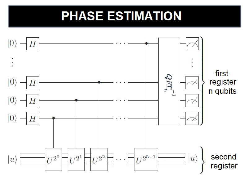
   Figure 2.12: Phase Estimation

   The first register prior to implementing the inverse quantum Fourier transformation can be expressed as:

   $$\frac{1}{2^{n/2}}\left(\lvert 0\rangle+e^{2\pi i2^{n-1}\phi}\lvert 1\rangle\right)\left(\lvert 0\rangle+e^{2\pi i2^{n-2}\phi}\lvert 1\rangle\right)\cdots\left(\lvert 0\rangle+e^{2\pi i2^{0}\phi}\lvert 1\rangle\right)$$ (2.107)

   $$=\frac{1}{2^{n/2}}\sum_{k=0}^{2^{n}-1}e^{2\pi ik\phi}\lvert k\rangle$$ (2.108)

   Subsequently, an inverse quantum Fourier transformation is applied on the first register, yielding:

   $$\frac{1}{2^{n/2}}\sum_{k=0}^{2^{n}-1}e^{2\pi ik\phi}\lvert k\rangle\xrightarrow{QFT_{n}^{-1}}\frac{1}{2^{n}}\sum_{k,l=0}^{2^{n}-1}e^{\frac{-2\pi ikl}{2^{n}}}e^{2\pi ik\phi}\lvert l\rangle\displaystyle=\displaystyle\frac{1}{2^{n}}\sum_{l=0}^{2^{n}-1}\left[\sum_{k=0}^{2^{n}-1}\left(e^{\frac{-2\pi il}{2^{n}}}e^{2\pi i\phi}\right)^{k}\right]\lvert l\rangle$$ (2.109)

   $$=\displaystyle\frac{1}{2^{n}}\sum_{l=0}^{2^{n}-1}\frac{1-e^{2\pi i(2^{n}\phi-l)}}{1-e^{2\pi i(\phi-l/2^{n})}}\lvert l\rangle$$ (2.110)

   The sum in the square brackets is a geometric sum and can be simplified. The resultant state contains the estimation of the phase $\phi$. Suppose $\phi$ can be expressed with n bits as $\phi=0.\phi_{1}\dots\phi_{n}$. Then, the exponential term $(2^{n}\phi-l)$ can be expressed as $(\phi_{1}\dots\phi_{n}-l)$ with l being an integer between 0 and $2^{n}-1$. Note that exponential terms are periodic in $2\pi i$ thus $e^{2\pi i1.\phi_{n}}=e^{2\pi i(1+0.\phi_{n})}=e^{2\pi i0.\phi_{n}}.$ The last term $l=2^{n}-1$ contains all digits of $\phi$ up to the $n^{th}$ digit, which determines the precision of the phase estimation protocol.

   The phase estimation protocol enables the estimation of the eigenvalue’s phase $\phi$ of a quantum system with an operator $\hat{U}$ and eigenvector $\lvert u\rangle.$ The output of the measurement of n qubits estimates the phase $\phi$ up to a precision $\propto n$.

   2.37   Variational Quantum Eigensolver

   So, now we come to the second approach. The point of this second approach, VQE, is to get by with a much poorer, worse quantum computer by not asking for quite as much, and we will see how that works by describing the algorithm. The point of this argument is to rely upon the variational principle, which in this context says that if we were given some state, psi, which is not the ground state. We measure the Hamiltonian’s expectation value, which is full total Hamiltonian with respect to that state. We will get some expectation value average energy, which is no smaller than the energy of the ground state. So, therefore, we might do something like introducing a bunch of parameters here. Let us call these $\theta$. So, $\theta 1$, $\theta 2$, $\theta 3$, and say we use the $\theta$ to manipulate the degrees of freedom we have in the input state to this expectation value. Then again, it will also be no smaller than that. So, we might define this thing as an expectation value of H parameterized by some $\theta$. we can do this on a classical computer, but the hardest part about the classical computation is preparing this state and then computing this matrix element of H with that state. the VQE algorithm proposes to do those two steps on a quantum computer. the rest, it does with a classical computer. So, here are the steps. Prepare psi of $\theta$, where $\theta$ it is controlled by a classical algorithm, and this is done on a quantum computer. ensure this H of $\theta$, and there are many ways of doing this measurement. One of which we will describe in a moment if we have time on a quantum computer. then, third, take this classical measurement result that we now have and run an optimization algorithm. For example, the Nelder-Mead simplex algorithm, or stochastic gradient descent, or we choose our favorite optimization algorithm, changing $\theta$ to minimize each of $\theta$. go back to the beginning, and this is done on a classical computer. So, now we have a hybrid, where we have a quantum computer executing some steps, and a classical computer executing some other steps. we can show that this kind of a variational expectation value is true even if we have a natty density matrix here, instead of a pure state. So, if our quantum computer starts to devolve and go not so, quantum on we halfway through, it still cannot give us an expectation value that is better than the ground state. there are various versions of these sets of theorems, which apply to variances in other quantities that we might want to measure. Thus, one can try to assert, although it is largely done without proof, that this argument will still work reasonably fine on a noisy quantum computer with not so good quantum bits. therefore, companies can deliver to we a product which is a quantum computer with poor quantum bits, and still expect we to pay a lot of money for it because it could run this algorithm and give we some result. There are not many proofs that it will do so, but it is a very compelling argument and a very interesting direction. there are now experimental results showing small one and two-qubit quantum computers doing exactly these steps, the variational quantum eigensolver. So, the challenge of this, there are two, we would point out most. First, does this expectation value converge? we have to rely upon this classical optimization algorithm to get we better and better values. However, we do not have proof that we got the lowest possible value or the desired ground state. Second, this state preparation. It is unclear how this state is prepared. There are some ideas on how to prepare this. For example, with adiabatic quantum computation. we start with a beginning Hamiltonian, which we can create, and try to construct an end Hamiltonian whose ground state is this state that we want to create. since we have this parametrized in principle, we have some means by which we can do that. This parameter, by the way, could be things, for example, like the adiabatic path that we use in the quantum computer. related to this first challenge is how we measure H., And one way people have done this is to measure the terms of H. So, we can say this is equal to the average expectation value of H1 plus H2, plus all the way up to however many terms there are in here. So, we can measure, in principle, the expectation value turn by turn in the Hamiltonian. if the Hamiltonian terms are simple, like Pauli matrices[22], we have a feasible way of doing it. Unfortunately, that means that we also now added the error from each one of these expectation values. So, the error can grow very rapidly as we are trying to estimate the expectation value this way. Still, the variational quantum eigensolver is different. we have not looked at any kind of algorithm like that in this section. How do we utilize a system with a quantum computer and a classical computer together so that we can get something of the best of both systems? How can we make them work in concert so that one handoff information to the other one so that now we can feedback and try to speed up, while only have a limited amount of quantum coherence and a limited number of qubits at our disposal? we think this is a fascinating topic. we want to leave us with that challenge, and we want to also leave us with the challenge of thinking about how we can relate Hamiltonians and quantum algorithms [76].

   Phase estimation determines the eigenenergies of a quantum system up to a specified accuracy. However, stringent requirements on the quantum processor’s performance, such as the available coherence time, limits the current applicability of this method as high accuracy requires long quantum circuits with many gates (high gate depth)[226, 77]. In contrast, quantum optimizers such as the variational quantum eigensolver (VQE) have more relaxed requirements on the quantum processor performance and work with shorter quantum circuits (“shallow depth”) contain parameterized, analog elements[55, 97].

   A VQE uses an iterative hybrid approach [224] to calculate the ground-state energy of a problem-specific Hamiltonian by creating a trial wave function on a quantum processor and measuring its energy with respect to the desired Hamiltonian. The trial wave function is made using a quantum circuit based on multi-qubit and single-qubit gates containing tunable parameters and optimized using a classical computer working in tandem with the quantum processor. An optimization loop repeatedly alters between quantum and classical processing until the optimal parameter set has been found, which generates the minimum energy corresponding to the ground state wave function.

   As explained in the section, the VQE protocol is initiated with a trial wave function $\Psi(\alpha)$ on a quantum computer. Here, $\alpha$ is the tuning parameter that will successively get optimized to yield the minimum energy. The quantum processor evaluates the expectation value of the trial wave function, $\langle\Psi(\alpha)|H|\Psi(\alpha)\rangle,$ where $H$ represents the problem-specific Hamiltonian, and $\langle H\rangle$ correspond to the energy of the prepared wave function with respect to the Hamiltonian. Generally, this requires repeated runs for the same parameter set, not just to obtain enough statistics but also to measure in all the different measurement bases specified in the Hamiltonian (a process often referred to as Hamiltonian averaging). A classical optimizer is then used to minimize the expectation value (energy) by varying the trial wave function through the parameter $\alpha$. The process repeats until E converges to a steady-state close or equal to the ground state energy $E_{0}.$

   Early demonstrations of VQEs using superconducting qubits simulated the ground-state energies for a hydrogen molecule $H_{2}$ [90], lithium hydride LiH and beryllium hydride $BeH_{2}$ molecule. A demonstration using trapped-ion qubits [133]also used VQE to simulate a hydrogen molecule $H_{2}$ and lithium hydride LiH., photonic qubits have been used to find the ground-state energy of a $He-H^{+}$ molecule[88, 96, 104].

   2.38   Variational Quantum Eigensolver (VQE)

   Let us start with the energy graph of a simple diatomic molecule. When the atoms are close to each other, the repulsion between the individual nuclei dominates the energy of the system and leads to an unstable configuration. At the other extreme is the case when the two atoms are dissociated. The point of minimum energy is the equilibrium configuration when the bond distance separates the atoms. Evaluating these energies to high accuracy is extremely crucial for accurately predicting chemical reaction rates and pathways and developing insights into molecular structure[104]. The evaluation of these energies essentially comes down to solving the Schrodinger equation, with the following electronic Hamiltonian, which captures the electronic kinetic energies and the Coulomb interaction between pairs of electrons and nuclei, as well as pairs of electrons. However, this eigenvalue problem is one with the exponential cost when addressed by classical computation. this was indeed one of the initial motivations for quantum computers, the idea that one could use a highly controllable programmable quantum processor to efficiently study and predict the properties of quantum systems of interest. The first step of such simulations, then, involves encoding the problem to the quantum processor, in the specific case, mapping the electronic orbitals onto qubits. One then needs an algorithm that solves the eigenvalue problem to evaluate the ground state energy. In this context, hybrid quantum-classical algorithms with short-depth circuits[90], such as the variational quantum eigensolver[96, 97, 100], are well-suited to the capabilities of existing hardware. Here, the trials, or guesses, to the ground state are prepared on the quantum processor, parametrized by some experimental controls $\theta$. The energy of these states is measured and fed to an optimization routine run on a classical computer that updates these parameters to attempt a new trial state. this is now run its iteratively until the energy converges towards its minimum value. It raises three important questions for implementing this algorithm. Are there encoding schemes that are efficient towards the number of qubits required? Are there trial states that are efficient towards the number of gates required while faithfully representing the ground state of the molecule? It is important since this can help reduce the effect of decoherence during state preparation. Finally, are classical optimization routines that can effectively deal with a large number of variational parameters and experimental lines? These were all important components of a recent experiment at IBM. Taking advantage of natural symmetries in the molecular Hamiltonian[104], we were able to encode eight orbitals of beryllium hydride onto a reduced number of 6 qubits at no loss of information. Also, we constructed trial states that used layers of untangling gates that are naturally accessible to the experimental hardware, which is then interleaved with arbitrary Euler rotations. The circuit dept or the number of entangling layers is then set based on the available quantum coherence of the hardware. Making efficient use of coherence time and qubit resources, these states are dubbed hardware-efficient trial states. Using such trial states, we were able to perform energy minimizations of up to 6-qubit Hamiltonians. Here is one such example. In the classical optimization routine, 13 Euler angles, which serve as the variation of parameters, are simultaneously updated as the local reading is approximated using solely two energy measurements by iteration, shown here in red and blue. The iterations are stopped once the energy flattens out towards its minimum. Using these techniques, we were able to address different electronic structure problems [194, 195, 20, 263, 98, 99] of fairly elementary molecules using 2 qubits for hydrogen, 4 qubits for lithium hydride, and 6 qubits for beryllium hydride. These are problems that are small enough to solve even on a laptop. However, a big motivation for this work is to be able to understand the sources of error and when addresses these problems using the normal paradigm of computing, using real quantum hardware. by comparing the experimental results, shown in these black dots with numerical simulations of the noisy device, we see the decoherence at insufficient circuit depth is some of the important sources of error. So, now this raises the question, in the absence of quantum error correction[27], is there a way to do something meaningful with near-term hardware? Is it possible to obtain estimates for, say, these energies in the absence of incoherent noise, despite using a noisy quantum processor? It turns out there are methods that we call error mitigation[212]. If there is an easy way to amplify the strength of the noise and measure the expectation values of interest, we can then use a powerful numerical technique Richardson extrapolation to obtain a zero-noise estimate. Here is a case of two wrongs making a right. In contrast to quantum error correction that has a resource requirement that is perhaps beyond near-term hardware, this error mitigation technique is fairly accessible since it does not require any additional quantum resources[209]. Now, is there a way for us to controllability amplify the strength of the noise? For instance, warming up the dilution refrigerator, which houses the superconducting processor[105, 148], certainly increases decoherence. However, there is not a precise way of scaling the noise strength. However, an alternate, more accessible approach involves rescaling the dynamics of the state preparation. It can be shown to be equivalent to amplifying the strength of the noise if the noise is constant over the duration of the rescale measurements. Let us now revisit the molecular simulation of lithium hydride with 4 qubits. The original experiments used just depth-one circuits to reduce the effect of decoherence. More recently, the mitigation of errors from decoherence enables the benefit of longer computations with increased circuit depth, to achieve accuracies that were otherwise believed to be beyond the scope of the noisy superconducting processor. Although discussed with specific examples of quantum chemistry, the variational algorithms [145] and error mitigation techniques discussed here can be extended to a host of different problems that rely on computations with expectation values problems in quantum simulation addressing fundamental particle physics and condensed matter physics, and even problems in optimization and machine learning [49, 187, 50, 52]. These techniques will likely be crucial to enhance the quality of quantum computation and simulation in this era of noisy intermediate-scale quantum computers.

   

   Figure 2.13: Newtonian Mechanics

   

   Figure 2.14: Hamiltonian Mechanics

   

   Figure 2.15: Schrodingers Equation

   

   Figure 2.16: Trotterization

   2.39   Introduction to Quantum Optimization

   In this section, we turn our attention to optimization problems and their implementation on a quantum computer. Optimization problems are ubiquitous in industry and government, for example, routing signals in electronics to minimize cross-talk, distributing financial portfolios to maximize profit while minimizing risk, or identifying the most likely nexus within a dense network of telephone calls. Such optimization problems with large numbers of variables and constraints are challenging to implement on classical computers. There are significant research efforts aimed at developing quantum optimization algorithms that may yield quantum enhancement.

   There are several approaches to quantum optimization. The first is adiabatic quantum computing and its related[109], restricted cousin, quantum annealing[175, 176]. In this case, a cost function is encoded into a Hamiltonian using a prescribed approach. The quantum device then seeks to minimize the cost function by finding the ground state of this Hamiltonian. A second approach is to use a universal, digital quantum computer to find a solution that satisfies (to the extent possible) a set of boolean clauses. We will discuss this section more about the advantages and challenges of these differing approaches.

   We do not always need exact solutions to optimization problems; approximate solutions are often “good enough.” For example, in establishing an optimal route that minimizes the distance one needs to travel between several cities separated by 100’s of kilometers, one probably would not distinguish between several high-quality solutions that differ by only a few meters or even a few hundred meters. Thus, there is intense interest in identifying quantum approximate optimization algorithms (QAOA) [21, 248] that feature quantum advantage in providing high-quality solutions, without necessarily obtaining the optimal answer. Such algorithms may be realizable on nearer-term, smaller-scale quantum computers, whether acting alone or as the co-processor working in tandem with a classical computer.

   Next, we discuss that the output of quantum computer was one value with a higher probability, and the question is can a simulation algorithm result in a distribution of probabilities? and the answer is yes it can. if there really is only one value, then that value has probability one. because we always normalize the probability to one. so, if any given answer is not obtained with unity probability. it means is that there are other answers floating around with lower probability. such that when we add up all the possible answers then the probabilities of all those answers is that we get one. So, in quantum simulations it could be depending on what we are simulating that we would get a distribution of many different answers with different weightings. the problem with that is we have to at any given instance or run the algorithm we are going to make a measurement projectively and get one of those answers out. so to estimate the probability of each one and sampling all different answers. we have to, identically prepare and repeat the algorithm many times. and if this solution space is exponentially large then that is going to take an exponentially long time. So that is not really the right way to ask a quantum computer a question. Rather, the simulations, or the optimizations, need to ask the questions in such a way that the solution space is not exponentially large, but reduced to either one answer, with high probability, or a set of answers, that all of which are high quality, so that it does not really matter which one we get. so, the example that we have given, we think, before, is that if we are trying to optimize, which route to take home from work, and it is 10 miles away, there may be a whole set of answers that are accurate enough that we do not care which one it is. Let us say that there are a hundred different ways we could get home, and they differ by 100 meters? and it is 10 kilometers to get from home, we know, from work to home. we do not care? it is only 100 meters difference. What matters is not off by a kilometer. So, in these types of cases, optimization problems, for example, there need not be, there may be one truly optimal answer, but in all likelihood, there may be many answers which are equally good from a practical sense. so as long as the algorithm is set up to find those answers, or that set of answers, samples any one with high probability, then it is fine. we can run the algorithm a few times, not an exponentially large number of times, if we can ask it a few times, and we start to sample some of these potential good solutions, and eventually, we gain some confidential cases, it is probably a good solution.

   2.40   Adiabatic Quantum Computing

   Optimization problems are ubiquitous in business, government, and our daily lives. They also tend to be hard problems to solve, because of the large number of variables and connectivity within the problem. In this section, we will discuss adiabatic quantum computing, one approach to addressing optimization problems. We will also discuss how adiabatic quantum computers are different from gate-model quantum computers.

   In the last section, we discussed several topics related to quantum Hamiltonian simulation, including methods like Trotterization [211], phase estimation, and variational quantum eigensolvers. In this section, we will turn the attention to quantum optimization algorithms. Optimization problems are ubiquitous, from supply transport optimization to sensor and satellite tasking, pattern recognition. Many important practical problems can be reduced to satisfy, in an optimal manner, as many constraints as possible. we will first discuss optimization problems and their implementation on an adiabatic quantum computer. we will then turn the attention to quantum annealers, machines that target classical optimization problems. lastly, we will look at Grover’s algorithm and how it works. at the end of the section, we will implement Grover’s algorithm on the IBM Quantum Experience [231]. To get started, let us first study adiabatic quantum computers and quantum optimization algorithms. Adiabatic quantum computing is an all-purpose approach to solving combinatorial optimization problems[264], or generally for finding the minimum of an objective function, using a quantum computer. we know that all systems in nature obey the Schrodinger equation. It is a first-order differential equation, which says that the wave function’s rate of change is proportional to the Hamiltonian operator times the wave function. So, adiabatic quantum computing uses the Schrodinger equation as the basis of the algorithm. It is distinct from the gate model in that sense because we are going to have continuous-time evolution. The quantum state is going to change continuously, as opposed to the gate model, where sequences of discrete transformations update the state. They are very closely related. However, in this case, we think it is a lot easier to think about how the algorithm works if we think in the context of the continuous-time evolution. Let us try to give us a feel for how the adiabatic algorithm works. we want to find the minimum of a complicated cost function. in general, there is no all-purpose algorithm that will guarantee to find the minimum of any cost function in all circumstances. We are trying to find something which we hope will work well in practice in situations we care about. So, the idea is this. We are going to attempt to find the minimum cost function by encoding the cost function in a quantum Hamiltonian. we are going to take a quantum Hamiltonian, whose ground state that is its lowest energy state we know, and we are going to prepare the quantum system in the ground state of this known Hamiltonian. Sometimes we call that the beginning Hamiltonian. If we look at this equation here, we see that the Hamiltonian that controls the evolution of the system has two parts, the beginning Hamiltonian and the problem Hamiltonian. Now, we are going to start the system off in the ground state of the beginning Hamiltonian, because the beginning Hamiltonian is something we know how to construct, and we know its ground state. then what we are going to do is slowly turn off the beginning Hamiltonian and slowly turn on the problem Hamiltonian. So, we are going to go from one to the other slowly. However, the problem Hamiltonian has been constructed so that its ground state encodes the solution to the minimization problem, which is the goal. we are going to take the system, and we are going to slowly change the Hamiltonian as the state evolves, according to the Schrodinger equation, the first equation we showed us. Let us give us a little example of how this might work. Suppose that we put a little ball in hand. it is just sitting there. Imagine it in our mind’s eye. it is sitting in it is in the minimum of a potential well formed by hand. Now we slowly move the hand. the little ball, as we can see in our mind’s eye, stays right there in hand. What is happened in that case is that we are changing the physical system, and we are dragging along the minimum energy configuration. Now, suppose that we put that little ball there, and we jerked hand. The ball would fall away. So, if we let the hand go slowly enough, we will drag along the little ball. the quantum system works in a very similar fashion. If we put a quantum state in Hamiltonian’s ground state, then we slowly change the Hamiltonian. If we go slowly enough, the Hamiltonian ground state will correspond to the evolving quantum state. In other words, we can shlep the ground state from the ground state of the beginning Hamiltonian to the ground state of the problem Hamiltonian, if we go slowly enough. that means that we have a way of finding the ground state, which corresponds to the minimum energy configuration, or the lowest value or the cost function that we sought. It will work, for sure, if we go infinitely slowly. Now, infinitely slowly requires an infinite amount of time. Thus, that is not a practical algorithm. So, the real question becomes, can we go slowly enough but not so, slowly that it is impractical, that we can bring the system to the place we want?

   Adiabatic quantum computing (AQC) is a quantum computing model that casts the problem of finding the solution of a computational problem into the problem of obtaining the lowest energy eigenstate of a specified Hamiltonian. Edward Farhi theoretically proposed it, Jeffrey Goldstone, Sam Gutmann, and Michael Sipser in 2000 [108, 215], as a general computational model, and it was later shown to be polynomially equivalent to universal, circuit-model quantum computation by Dorit Aharonov and colleagues in 2004 [109].

   The physical principle governing AQC is the adiabatic theorem. Essentially, this theorem states that a physical system will remain in its lowest-energy eigenstate under sufficiently slow changes to the parameters of its Hamiltonian. This fact can be put to computational use by initializing a computer in the ground state of a known Hamiltonian, called the “initial Hamiltonian”, and then adiabatically evolving its parameters into the “problem Hamiltonian” with a ground state that encodes the solution to the computational problem. The slow evolution of the system is intended to guarantee that the system remains in the ground-state throughout this process. However, as indicated below, this is generally not achievable for problems of practical size due to the “minimum gap” problem.

   An adiabatic quantum algorithm [108] for a given computational problem is comprised of choice for the initial Hamiltonian, the evolution path, and Hamiltonian. None of these choices are unique (except, possibly, the problem Hamiltonian). The initial Hamiltonian is generally chosen to have a known ground state, and simple implementation, e.g., all spins aligned along the X-axis of the Bloch sphere (state $|+\rangle=\frac{1}{\sqrt{2}}\left(|0\rangle+|1\rangle\right)$ due to an interaction with a large control field. The problem of interest is then embedded onto the hardware to create the problem Hamiltonian, within the constraints imposed by the available qubits and their interactions. Lastly, an evolution path from the initial Hamiltonian to the Hamiltonian’s target is chosen, and ideally, this choice respects the conditions imposed by the adiabatic theorem. Using this approach, small-scale adiabatic quantum algorithms for search, factorization, and optimization have been experimentally demonstrated with nuclear spins and magnetic resonance, superconducting qubits, and photonic qubits [97].

   The choice of initial Hamiltonian, evolution path, and problem Hamiltonian together determine how rapidly the system can be evolved and, thus, determine the runtime complexity of the adiabatic algorithm. In principle, the shorter the runtime, the more efficient the algorithm. However, running the algorithm faster than is allowed by the adiabatic theorem decreases the chances of obtaining a correct solution at the end of the evolution process.

   In fact, for larger problems of practical significance, adiabatic quantum algorithms generally cannot be implemented without the system leaving the ground state. It is because of the “minimum gap” problem. As the system evolves from initial to problem Hamiltonian, the energy levels eventually come close and form an avoided crossing, i.e., come close but do not quite touch. One can intuitively think of this as a “crossing point” where the system leaves its initial-Hamiltonian-like nature behind and starts adopting problem-Hamiltonian-like characteristics. In physics jargon, this is essentially a phase transition [88].

   The problem is that the gap becomes smaller and smaller as the problem size increases. This results in two key issues. First of all, even in the absence of noise, the system must evolve more slowly through the gap region as the gap gets smaller in order to maintain adiabaticity. If the system evolves too quickly, the system will effectively “jump” to the excited state via a nonadiabatic process called a Landau-Zener transition. Avoiding Landau-Zener transitions requires longer evolution times, thus increasing the time-to-solution and slowing the computation.

   Second, and more insidious is that there is always some level of noise. As the gap size decreases, noise from the thermal environment and noise from the control fields implementing the evolution will drive transitions from the ground state to the excited state. For example, once the gap energy becomes smaller than the thermal energy $k_{\textrm{B}}T$ at temperature T, the environment will drive transitions. Thus, for large enough problems, it will be practically prohibitive to evolve the system while remaining in the ground state.

   Given that an adiabatic quantum computer will leave the ground state at some point during its evolution (for a sufficiently large problem), one may wonder if that destroys any potential for quantum enhancement. After all, what if the computer could return to the ground state after passing through the minimum gap region?

   In 1998, Tadashi Kadowaki and Hidetoshi Nishimori proposed such a quantum annealer to solve classical optimization problems. A quantum annealer leverages quantum tunneling [23]and dissipation (relaxation processes) to return a system to its ground state (or a lower-energy state) after passing a small avoided crossing. While such quantum annealers seemingly bypass many of the constraints imposed by an adiabatic quantum computer, there is no evidence that quantum annealing computers feature quantum enhancement to date[191, 192, 177, 178, 179].

   2.41   Adiabatic QC

   How do adiabatic algorithms solve optimization problems? In this section, we will discuss the adiabatic algorithm [215], how it is used to minimize “cost functions,” and how it is implemented using spin Hamiltonians.

   Let us go back to the concept of adiabatic evolution, but let us be a little bit more specific now. So, we want to imagine that we want to find the minimum of a cost function, which is defined over bit strings. that cost function is the sum of terms, each of which depends on a subset of the bits and has a value of 1. Let us say, on certain assignments of those bits in the subset, and has the value 0 on other assignments. For example, if an individual term might look at 2 bits and it will say, if the 2 bits agree in their value, we are going to give it the value 1, but if they disagree, the function has the value of 0. So, now, we want to imagine that the optimization problem is to find the minimum of a function, which is a sum of terms, each of which acts on a few bits. finding the minimum of such a function, in general, is what we call NP-hard. It is not believed that there is any kind of classical time algorithm that can, in polynomial time, solve that problem in general. Nonetheless, we are going to attempt the quantum approach to it. So, the first thing we are going to do is to find what we told us before was the problem Hamiltonian. the problem Hamiltonian we are going to take to be diagonal in the computational basis, so, when the problem Hamiltonian acts on a ket with the string z in it, it will give the value of the cost function times the cat. So, it is diagonal in the computational basis. Note that the minimum string that achieves the minimum value of the cost function can be viewed as the ground state of this particular quantum Hamiltonian because it is diagonal on a computational basis. Now, we need to take a beginning Hamiltonian too. from that, we typically use a magnetic field in the x-direction. If we have a magnetic field on a single spin a half particle and it is pointing in the x-direction, it is represented by the operator. we will take it to be minus $\sigma$ x so that the state in the x-direction is the minimum with the value minus 1. So, the Hamiltonian we are going to take for the beginning Hamiltonian is the sum, a minus in front, the sum of the $\sigma$ x is one for each qubit. That is a very simple Hamiltonian. it is very easy to initialize a quantum state as the ground state of that Hamiltonian because all we have to do is take the spins and line them up in the x-direction. Then we are automatically in the ground state of the beginning Hamiltonian. So, now for all full evolution, we are going to take a Hamiltonian that it interpolates between the beginning Hamiltonian we prescribed and the problem Hamiltonian. So, that is all very simple to write down. Not only is it simple to write down, but it is also easy to imagine implementing such a thing in the lab or on a quantum computer because the terms in the problem Hamiltonian are a sum of local terms diagonal in the computational basis. the beginning Hamiltonian is just a magnetic field in the x-direction. So, we can imagine building this thing. what the D Wave company did is build a machine that runs this algorithm. They chose to implement the quantum adiabatic algorithm because it was simple to imagine building a device that could do that. the way we have discussed it, it is kind of an all-purpose minimizer. So, we now have gone as far as to see that we can have a specific implementation of the adiabatic algorithm. So, What is the killer here? What slows it down? What is the thing that makes it hard to implement this in reality and means that it is hard to show the algorithm works all the time? Furthermore, that has to do with how slowly we have to go to guarantee that we are going to go to the place we want to end up at. that slowness is determined by something we call the minimum gap. At the beginning of Hamiltonian, we have a magnetic field in the x-direction. If we flip a single spin, the energy of that single spin goes from Let us say minus 1 to plus 1. So, the energy difference is 2. That is a big energy difference between the ground state and the first excited state. In the problem Hamiltonian, we told we that all terms were zeros and ones, because the cost function, the way we happened to define it, was a sum of terms, which were all 0 or 1. So, that means that the energy difference between the ground state and the first excited state is Let us say, 1 or 2, but it is going to be an integer. However, as the system evolves, we can track the ground state energy and the energy of the first excited state. we find in these situations that as we move along, the two approach each other, coming very, very close. then they are going to spread out back to that integer at the end. the question is, What is that value, the smallest energy difference between the first excited state and the ground state? we call that the gap. the runtime of the algorithm is determined by the gap. The minimum runtime of the algorithm scales like 1 over the minimum gap squared. That is just a little math fact, which we could establish. The whole issue from a physics point of view in the adiabatic algorithm is, does the system, as it evolves, make the energy difference between the ground state and the first excited state get too small? Because if it is too small, the run time required to stay in the ground state is too big. So, one of the things we have to study when we think about adiabatic algorithms is the gap between the first excited state and the ground state as the system evolves.

   2.42   Quantum Approximate Optimization Algorithm

   In this section, we continues discussion of optimization algorithms [215]. Here, we will discuss combinatorial search problems and the quantum approximate optimization algorithm (QAOA)[21, 265].

   we have already established what we think throughout this section, and most of us know that optimization is a key problem in all of computer science. Now, let us get a little more specific and think about what optimization means in combinatorial search. There we have a problem defined on bit strings. we have clauses or constraints, which look at subsets of the bits. for certain assignments of the bits, those clauses are satisfied. for others, they are not. What we want to do in combinatorial optimization, is find a string that can satisfy as many clauses as possible. Often we cannot satisfy all the clauses. Because the clauses have intrinsic contradictions, so that assignments for one clause that satisfy it, force other clauses not to be satisfied. The question then becomes, what is the string that satisfies, Let us say, as most clauses as possible? Now that is very ambitious. Because satisfying the most clauses as possible, that is NP-hard. if we could do that in general, we would have a huge computer science breakthrough. Most people believe that there could be no polynomial-time algorithm for that. So, instead, we are going to come back a little bit and look for a string that satisfies many of the clauses, or as many as the algorithm can produce. So, what we are looking for is a good solution, not the best solution. we are looking for a good string, not the best. In that case, if our good solution is very, very close to the best, it is as good as the best; but if it is a little off, it could still be of great value to us. Thus, what we are going to be discussing is an algorithm that is an approximate optimizer. It is looking for approximate solutions in the sense we just said. we are going to try this with a quantum algorithm. However, the quantum algorithm is now not like in the adiabatic, and it is going to be based on a continuous-time evolution. However, rather it is going to be in the gate model, which means we are going to apply a sequence of discrete unitary transformations to an initial state, and then make a measurement, and hope that that measurement gives a string that satisfies a high fraction of the clauses that could be satisfied. So, in order to build this up, we need a few ingredients. we need the initial state and the unitaries that we are going to apply. So, let us think about that. well, for the initial state, what we are going to take is all the spins lined up in the x-direction. the reason we like that is we probably already know that if our spin is in the x-direction, it is a uniform superposition of up and down in the z. In other words, it is an equal combination of 0 and 1. So, if all our spins are lined up in the x-direction, our state is a uniform superposition of all possible bit strings. that is kind of a good place to start. Because we have everything in there when we begin, in the computation basis. Now we are going to apply two operators. The first operator is going to depend on the actual operator-valued cost function. The cost function acting on a string gives us the number of clauses satisfied by the total that string. That is an easy-to-compute function. However, we could promote that function to a quantum operator, and that quantum operator acting on the ket labeled by the bit string z will be the function, which is the number of satisfied clauses times the ket. So, this operator-valued cost function is diagonal in the computational basis, and it is easy to construct. However, it is a Hermitian operator. we would like to apply a unitary transformation that depends on it. So, we are going to introduce a parameter, $\gamma$. we are going to write down the unitary here, e to the minus i $\gamma$ times that cost function. So, this object is a unitary transformation, which we can easily apply to any state. it depends on a parameter, $\gamma$, which we will discuss more later. Now the next operator, which we would like to apply again, there is much room for choice. However, we make a choice that will depend on the operator, which we call B, which is the sum of the $\sigma$ x’s, the sum of the Pauli operators in the x-direction. That is an operator, which we discuss in the adiabatic case, we call the beginning Hamiltonian. This operator B, which is the sum of the $\sigma$ x’s, is easy to construct. However, now what we want to do, though, is make a unitary operator, which depends on that. we are going to do that by writing e to the minus i $\beta$, which is the parameter we have just introduced, times the operator B. So, this operator, if we look at it, e to the minus i $\beta$ B, since each term in B is a $\sigma$ x, what it is doing is rotating the spins around the x-direction by an angle, $\beta$. So, now we have the two building block unitary operators, each of which depends on one parameter. So, the algorithm consists of the following. Start with the initial state, which we already described. Choose $\gamma$. Apply the unitary e to the minus i $\gamma$ C to that state. Then choose the $\beta$. Apply either the minus i $\beta$ B to the state, and now measure in the computational basis. we get out a string. now, What is interesting is that we can show that for certain problems, we can find values of $\gamma$ and $\beta$ such that the string that is produced will satisfy a high fraction of the clauses. we are not going to show we now how we find the $\gamma$ and $\beta$ to do that. However, that can be done for certain problems. in fact, for one problem, called MAX-CUT, when we first introduced this algorithm in 2014, we were able to show that we could achieve a restricted version of MAX-CUT [266]. This certain approximation ratio was better than we would get if we just picked a string at random. Now we could say, so, what? we did a little better than random guessing. However, we managed to show that this worked in every case, no matter how big the instance was, no matter how many bits or qubits were involved. With the right choice of $\gamma$ and $\beta$, we were guaranteed to get a good answer. So, in this case, we were able to show that the quantum computer would perform at a certain level, even on instances that we had not yet seen. The factoring algorithm has that great virtue. we know that if we had a functioning quantum computer, no matter what integer we give, it will be able to find its factors. Thus, we were able to show that we could get an approximation ratio that beat random guessing, no matter what we gave it. Nevertheless, we were not beating the best classical algorithm. then we looked at another problem called E3LIN2. We could be much more specific. However, for now, just go with the story. we looked at this problem, E3LIN2. We showed that with just this shallow depth circuit, we could achieve an approximation ratio, which is 2014 beat the best classical algorithm for this problem. Now at that moment, We had a quantum algorithm that beat the best classical algorithm for a certain task in all cases. The word of this spread. The way it spread was basically because Scott Aaronson blogged about it and said there was this neat new quantum algorithm, which got the classical computer scientists and the non-quantum people together. 10 of them ganged upon, and they devised a classical algorithm that beat the quantum algorithm for this task. Nevertheless, what was interesting there is we got a competition going between the classical and the quantum. at this moment, in terms of provable worst-case performance guarantees, the classical algorithm is outperforming the QAOA. The QAOA is the Quantum Approximate Optimization Algorithm. Now we can go further with the QAOA than we have already outlined. Because of the way we have outlined it, it is a very simple algorithm with just two unitaries. we apply the first one, then the next one, then we measure. Nevertheless, we can go further. we can apply the first one and then the second one. Then we can apply the first one again with a different parameter. then, we can apply the $\beta$ dependent operator with a different parameter. Then if we keep going, by alternations of those two operators, it turns out that we can only improve the performance of the algorithm. Now we have had trouble from a technical point of view showing how much that improvement consists of. It has been too hard for us to analyze it beyond the very shallowest depth circuits that we did. However, we optimistic that when we run a near term quantum computer, if we apply this algorithm which should be fairly simple to do because it is a shallow depth gate model with simple-to-construct operators; that we might discover that there are parameter choices for which the solutions we get are quite good, even as good as what we get from classical algorithms, even better. So, we think that applying the Quantum Approximate Optimization Algorithm to near-term quantum devices is a definite avenue for this community to go down. we look forward to seeing the algorithm run on any platform capable of running it.

   A combinatorial optimization algorithm finds solutions to a problem subject to a set of constraints, and the optimal solution is the one that satisfies the largest number of constraints.

   The problem is defined by an object function C(b), which is a sum of m constraint clauses $C_{\alpha}$, where $\alpha=1...m.$ Each clause is a Boolean function that captures one specific constraint of the optimization problem. The Boolean functions are constructed from n Boolean variables $b_{1}\dots b_{n}$, which together form an n-bit string b, and there are $2^{n}$ such strings. Note that not all Boolean variables need to be used in every clause, and in general, they are not. If a given b satisfies a clause, then $C_{\alpha}(b)=1$ according to the Boolean function it represents; otherwise, $C_{\alpha}(b)=0$.

   The $b=b_{\textrm{opt}}$ that maximizes the object function $C(b)$,

   $$C(b_{\textrm{opt}})=\sum_{\alpha=1}^{m}C_{\alpha}(b_{\textrm{opt}})\geq\sum_{\alpha=1}^{m}C_{\alpha}(b\neq b_{\textrm{opt}})$$ (2.111)

   Is the optimal solution (or, an optimal solution if more than one solution exists). If all clauses are satisfied, $C(b_{\textrm{opt}})=m,$ but this is not required.

   In general, evaluating the optimal solution is a hard problem. An approximate solution that is not necessarily optimal but is still of reasonably high quality is sufficient for many optimization problems and maybe computed more efficiently. The quantum approximate optimization algorithm (QAOA) is proposed to find approximate solutions to a combinatorial optimization problem.

   QAOA is a hybrid approach that utilizes a digital quantum computer (QC) to evaluate the object function and a classical optimizer (CO) to update trial solutions to optimize the object function. The iterative process on n qubits approximated with p optimization steps can be summarized as follows:
   $\displaystyle 1.\leavevmode\nobreak\ \leavevmode\nobreak\ \leavevmode\nobreak\$ CO: generate initial set of angles $\gamma_{1}$ and $\beta_{1}$ to optimize the object function
   $\displaystyle 2.\leavevmode\nobreak\ \leavevmode\nobreak\ \leavevmode\nobreak\$ QC: create superposition of $n$ qubits in computational basis ground-state
   $\displaystyle 3.\leavevmode\nobreak\ \leavevmode\nobreak\ \leavevmode\nobreak\$ QC: rotate qubits on Bloch sphere by angles $\gamma_{1}$ (z-axis) and $\beta_{1}$ (x-axis)
   $\displaystyle 4.\leavevmode\nobreak\ \leavevmode\nobreak\ \leavevmode\nobreak\$ QC: measure qubits in computational basis and evaluate the object function
   $\displaystyle 5.\leavevmode\nobreak\ \leavevmode\nobreak\ \leavevmode\nobreak\$ CO: generate new set of angles $\gamma_{2}$ and $\beta_{2}$ to optimize the object function
   $\displaystyle 6.\leavevmode\nobreak\ \leavevmode\nobreak\ \leavevmode\nobreak\$ QC: create superposition of $n$ qubits in computational basis ground-state
   $\displaystyle 7.\leavevmode\nobreak\ \leavevmode\nobreak\$ QC: rotate qubits on Bloch sphere by angles $\gamma_{1},\gamma_{2}$ and $\beta_{1},\beta_{2}$
   $\displaystyle 8.\leavevmode\nobreak\ \leavevmode\nobreak\ \leavevmode\nobreak\$ QC: measure qubits in computational basis and evaluate the object function
   $\displaystyle\vdots\leavevmode\nobreak\ \leavevmode\nobreak\ \leavevmode\nobreak\ \leavevmode\nobreak\$
   $\displaystyle 4p-3.\displaystyle\text{CO: generate new set of angles $\gamma_{p}$ and $\beta_{p}$ to optimize the object function}$
   $\displaystyle 4p-2.\displaystyle\text{QC: create superposition of $n$ qubits in computational basis ground-state}$
   $\displaystyle 4p-1.\displaystyle\text{QC: rotate qubits on Bloch sphere by angles $\gamma_{0},\gamma_{1},\dots,\gamma_{p}$ and $\beta_{0},\beta_{1},\dots,\beta_{p}$}$ $\displaystyle 4p.\leavevmode\nobreak\ \leavevmode\nobreak\ \displaystyle\text{QC: measure qubits in computational basis and evaluate the object function}$

   The algorithm is composed of two types of operators constructed with unitary quantum gates to rotate the qubits by angles $\gamma$ and $\beta$.

   $$C(b)=\sum_{\alpha=1}^{m}C_{\alpha}(b)\displaystyle\rightarrow\displaystyle U(C,\gamma)=e^{-i\gamma C}=\Pi_{\alpha=1}^{m}e^{-i\gamma C_{\alpha}}$$ (2.112)

   $$B=\sum_{j=1}^{n}X_{j}\displaystyle\rightarrow\displaystyle U(B,\beta)=e^{-i\beta B}=\Pi_{j=1}^{n}e^{-i\beta X_{j}}$$ (2.113)

   The operator C is based on the object function C(b), and it conditionally rotates qubits by an angle $\gamma$. For example, a clause $C_{\alpha}=\frac{1}{2}(-Z_{j}Z_{k}+1)$ rotates qubits j and k by an angle $\gamma$ around the z-axis if they are in opposite states. Therefore, only qubits complying with the clauses of the objective function are affected by the rotation.

   The second operator, B, applies a rotation of angle $\beta$ around the x-axis to all qubits. Note that states co-aligned with the x-axis remain unchanged for an X-rotation.

   An initial state $\lvert\psi\rangle=\frac{1}{\sqrt{2^{n}}}\sum_{s=1}^{2^{n}}\lvert s\rangle$ is iteratively rotated conditionally around the z-axis, and then around the x-axis, to reach a particular location on the two-dimensional Bloch sphere. The measured resulting state after p optimization steps is:

   $$\lvert\vec{\gamma},\vec{\beta}\rangle=U(B,\beta_{p})U(C,\gamma_{p})\cdots U(B,\beta_{1})U(C,\gamma_{1})\lvert s\rangle$$ (2.114)

   It can be shown that the expectation value of the object function improves with additional iterations and ultimately maximizes it. The performance of the underlying quantum processor usually determines the approximation accuracy.

   $$\max_{\vec{\gamma},\vec{\beta}}\langle\vec{\gamma},\vec{\beta}|C|\vec{\gamma},\vec{\beta}\rangle=M_{p}\geq M_{p-1}\leavevmode\nobreak\ \leavevmode\nobreak\ \Rightarrow\leavevmode\nobreak\ \leavevmode\nobreak\ \lim_{p\rightarrow\infty}M_{p}=\max_{z}C(b)$$ (2.115)

   The algorithm’s key element is the ability to conditionally project qubits on arbitrary locations on the Bloch sphere via iterative rotations induced by two distinct unitary operators. Each iterative step starts with a new set of classically optimized angles based on the qubit measurement of the prior step. A sufficient number of repetitions approximates the object function C(b), and the measured qubit state reflects the approximately optimal bit string b.

   There was a question about quantum algorithms, Is it always possible to transform any classical equation or algorithm into a quantum equivalent, or vice-versa, a quantum equation into a graphical tool, or back into a classical equivalent, The answer is yes, if we have a universal, fault-tolerant quantum computer, it is universal, and in principle, it can perform any algorithm, quantum or classical. Now, the key here though is that, the quantum computer may do no better than a classical computer, and oftentimes, it may do far worse, because it runs at a much slower rate, it does not have quantum advantage for that particular type of problem. so, although in principle it can do it, it may not be any better than a classical computer, and in fact, may be slower. Now similarly, we can take a quantum equation, or quantum algorithm, and we can simulate that, or implement that, on a classical computer, but to do that, we need to discretize the problem. We often need to make some assumptions, truncate the problem, reduce it down in some way so that it is tractable to implement on a classical computer and in doing that, we lose information, we lose fidelity. that is why it is generally hard to implement quantum algorithms, or quantum systems, to simulate quantum systems on a classical computer. Now, we could do it in full glory, but then that takes the age of the universe? it is this type of problem if we want to do it and simulate it, with the highest possible fidelities on a classical computer, it is going to take way too long, or it takes way too much memory to implement or to be practicable. If we cut down the problem so that we can do it on our classical computers, then we do not get accurate answers? And so, this motivates why we need to have a quantum computer. Now, is it always possible to transform quantum equations into its equivalent in a graphical tool set, like we have experienced with the IBMQ Quantum Experience. In principle, yes, but, a graphical user interface is an abstraction, so it is a convenience that we build in to, our human-computer interfaces, it is a tool. So, the graphical interface is limited to the extent that some of these programs has capability into it. so, perhaps there are gate operations that are not represented yet in their full generality in that graphical user interface. So it is in principle possible, but this is one reason why we do programming, using programming languages, rather than using a GUI interface, is because we can do operations with more generality when we do a lower level of programming rather than a higher level of graphical user interface. But as an in-principle, sure, there is nothing that prevents us from implementing everything that we would possibly calculate or program into a graphical user interface. It just may become bulky, and it needs to be designed very well, so that human-computer interface is still efficient with all that information.

   2.43   Quantum Annealing: Concept

   How are quantum annealers different from adiabatic quantum computers? Furthermore, how are they used to solve optimization problems? In this section, we will discuss quantum annealers.

   In the previous section, we discussed a paradigm of quantum computing known as adiabatic quantum computation. In this section, we are going to introduce another related quantum computing paradigm called quantum annealing. As we will see, quantum annealing bears many similarities to adiabatic quantum computation, though with a few key differences. First, recall that adiabatic quantum computation is a form of analog quantum computing. That is, rather than digitizing the computation into discrete gates, AQC relies on the continuous transition of a quantum system from the ground state of one Hamiltonian to the ground state of another. While it is true that adiabatic quantum computation is a provably viable method of universal quantum computation[75, 232], ACQ presents a serious practical challenge. In order for the computation to succeed, the system must remain in the ground state for the duration of the computation. If the evolution is not truly adiabatic, and the system ends up in an excited state at the end of the protocol, the computation fails. Unfortunately, this is an extremely hard condition to avoid in any realistic quantum computer. To see this, let us consider what the system’s energy levels might look like as we perform the computation. In particular, Let us focus on the energy gap between the ground state of the system and its first excited state. As the Hamiltonian of the system changes throughout the computation, the gap between the ground and excited states also changes, and in general, it can become very small. It is where the trouble starts. For any physical system at finite temperature, the environment around the qubits generates thermal photons with an energy proportional to the environment’s temperature. When these photons encounter the qubits, their energy is absorbed, and the system has some probability of being excited to a higher state. The smaller the gap with respect to the photon energy, the higher the probability that excitation will occur. If we want to reduce the probability of an excitation occurring for a fixed gap size, we need to cool the system to a temperature much lower than the energy gap between the qubit states. It is precisely why we operate superconducting qubits in a dilution refrigerator cooled to a temperature of around 10 millikelvins. For typical superconducting qubits, the gap between the bare qubits’ states is on the order of 5 gigahertz, which corresponds to a temperature of around 250 millikelvins. By operating the qubits in an environment order of magnitude colder, we dramatically reduce the probability of an unintentional excitation occurring during the computation. Unfortunately, as we change the Hamiltonian during an adiabatic quantum computation, new avoided crossings will open up between the states, which can be much smaller than the energy gaps between the barer qubit states. If we want to avoid transitioning across these small gaps in the case, say, of a superconducting annealer, we would need to engineer a refrigerator that operates much colder than 10 millikelvin, which is not practical given current cryogenic technology [110]. this type of problem generalizes other qubit technologies as well. there is a second problem. As we evolve the computer through a small gap region, if we sweep through the gap too quickly, we can effectively jump to the excited state. It is called a Landau-Zener transition. So, even if we could operate the computer at zero temperature, we would need to evolve the system sufficiently slowly to accommodate smaller and smaller gaps and thereby increase the time to solution. So, although adiabatic quantum computation can, in principle, be universal, it has major drawbacks related to the small gap sizes that occur at larger problem sizes. Given this reality, it is natural to ask, what happens if we allow the computer to leave the ground state during the evolution. Can it return to the ground states, or even a lower excited state, through quantum tunneling and relaxation processes? Furthermore, more importantly, is leaving the ground state consistent with the quantum-enhanced operation? Quantum annealing is an adiabatic quantum computer that has left its ground state at some point during the evolution. conceptually, a combination of quantum tunneling and relaxation processes are leveraged to allow the computer to return to its ground state, or at the very least, a lower energy state. However, to date, there was no proof or evidence that the quantum and dissipative dynamics in quantum annealing could then forward a quantum enhancement for a general class of problems. It remains an open research question. Much like AQC, the principle of quantum annealing involves evolving a quantum state according to some time-dependent Hamiltonian such that the state of the system at the end of the computation encodes the result of the problem of interest. However, unlike ACQ, which is universal and can, in principle, implement any quantum algorithm, quantum annealing is designed only to solve a particular class of computations known as classical optimization problems. we deal with classical optimization problems in every industry and throughout the daily lives. For example, What is the best portfolio of stocks to maximize return on investment? What is the best fighter jet designed to minimize drag? Or to use a more mundane example, What is the best path home from work? The key to an optimization problem is that there are many potentially viable answers to a given problem. For example, many paths will take us home from our office. The goal of an optimization problem is to find the most efficient solution from amongst all the possible solutions. we quantify this by introducing a cost function, which tells us the relative efficiency of a solution. For the commute home, the cost function could be the time it takes to get home if we followed a particular route. Alternatively, it could be the amount of gas we use. Whatever we are optimizing against, the optimal solution tells us the one that minimizes the cost function. although there may be a truly optimal solution, it is very often the case that there are several nearly optimal solutions that are all, in practice, very good. Commutes that differ by a few meters on 10 kilometers or differ by a few drops of gas on a liter are essentially interchangeable. the hope for these kinds of problems is that leaving the ground state may be fine if we end up in a reasonably low energy state. To map an optimization problem onto a quantum annealing problem, we make use of a particular Hamiltonian known as an Ising Hamiltonian. The Ising Hamiltonian was first formulated in the context of quantum magnetism between atomic spins. For a system of physical spin 1/2 particles, the Ising Hamiltonian tells us the energy of the spins as they interact with external magnetic fields plus the energy of the magnetic interactions between pairs of spins. So, how can this physics problem be used for optimization? As it turns out, we can use the Ising Hamiltonian to encode so,-called classical optimization problems[19]. By choosing the right combination of interaction strings between spins, we can mimic the cost function of the problem we are interested in. When we encode this optimization problem into the Ising Hamiltonian, we then find that the Hamiltonian’s energy levels corresponding to the possible solutions to the optimization problem with the energy at each level corresponding to the value of the cost function for that particular solution. Higher energies incur higher penalties. The goal of quantum annealing is to engineer a qubit system with an Ising Hamiltonian corresponding to the optimization problem of interest [190]. we then want to evolve the system such that it ends up in a low-energy eigenstate of this Hamiltonian at the end of the computation. The lower the energy of this final stage, the more optimal the solution. To perform this evolution, we start by initializing the system in the ground state of a much simpler Hamiltonian. Conventionally, this Hamiltonian is the sum of the x operator acting on every qubit, which is analogous to having an array of spin 1/2 particles in a global magnetic field pointing transversely to the spins. When we work out the math, we find that the ground state of this Hamiltonian is straightforward. It is the state where all the qubits are in the plus x state on the equator of the block sphere, which is a relatively easy state to the initialize system in. Once we prepare the system in the ground state of this initial Hamiltonian, we gradually reduce the strength of this initial Hamiltonian and turn on the Hamiltonian, which encodes the optimization problem. In the ideal case, the system evolves adiabatically and remains in the ground state throughout the evolution. It would be an adiabatic quantum computer simulating an Ising Hamiltonian. Ideally, at the end of the evolution, the system would still be in the ground state of the problem Hamiltonian corresponding to the solution, which minimizes the cost function. In other words, we would find the absolute shortest route home. However, as discussed at the beginning of this section, it is very unlikely that we will remain in the ground state throughout the computation. It does not necessarily ruin the computation. Because every energy state of the problem Hamiltonian corresponds to a possible solution, even if we exit the ground state and end up in an excited state at the end of the computation, this excited state may still give us a useful answer to the optimization problem. The question is, how good is this answer. Unfortunately, while quantum annealing relaxes the constraint that we stay in the ground state, it makes no guarantees that the result we arrive at is any more optimal, or any more efficiently found, than the result we might calculate on a classical computer. As such, unlike AQC, quantum annealing can make no provable claim to either universality or a quantum enhancement, and there is no demonstration to date of quantum enhancement for a class of optimization problems. That said, even if a quantum annealer ends upscaling with problem size like the classical computer, it may still be useful if it offers a significant advantage over existing classical computing alternatives. However, this also has yet to be demonstrated. Nonetheless, there is tremendous interest in quantum annealers because optimization problems are ubiquitous. while large-scale universal quantum computers are still a long way from commercial reality, the first generation of commercial quantum annealers designed by D-Wave currently boasts up to 2,000 qubits[128, 189]. while the D-Wave system has yet to demonstrate quantum enhancement for a general class of optimization problems [182], these machines, as currently constructed, only explore a small part of the quantum annealing design space[188]. As work gets underway to design the next generation of quantum annealers, it remains an open question if systems with higher quantum coherence and more sophisticated qubit connectivity might demonstrate a truly conclusive quantum enhancement.

   Quantum annealing (QA) is a method for finding solutions to classical optimization problems. It is essentially an adiabatic quantum computer that is allowed to leave its ground state during its evolution. Then, through a combination of quantum tunneling and relaxation, the system finds its way back to the ground state (or a lower-energy state), which encodes an (approximate) solution to the optimization problem.

   Quantum annealing borrows its name from thermal annealing. For example, in metallurgy, annealing is a process by which a metal is heated such that it is physical shape and composition can be modified. Then, upon cooling, the metal relaxes into this new shape and composition, from which it will not change unless heated. Loosely speaking, the thermal fluctuations present during the heating process enable the metal to reconfigure into an alternate, advantageous configuration.

   To gain insight, it is instructive to consider a classical algorithm called simulated annealing (SA)[267], which uses a thermal activation model to find approximate solutions to optimization problems. Intuitively, SA algorithms seek to replicate thermodynamics, where the cost function is encoded into the total energy of the system. The algorithm seeks to find a low-energy configuration as a parameter analogous to temperature T “reduced” to zero. Operationally, each iteration of an SA algorithm begins with a valid solution with energy E and randomly selects another solution near the current one. The new solution can either have a higher $(E^{\prime}>E)$or lower $(E^{\prime}<E)$ energy, where E’ is the energy of the newly selected solution. In one of the most basic implementations of SA, if $(E^{\prime}<E)$, then the new solution is chosen as the starting point for the next iteration. However, a key feature of SA is that even when $E^{\prime}>E$, although representing a less optimal solution, there is a non-zero probability that the algorithm will use it in the next round. It is intended to mimic thermal fluctuations transiently exciting a physical system, and it helps the algorithm escape from local minima in the potential landscape. The algorithm starts at “high temperature”, and the probability of keeping these $E^{\prime}>E$ solutions is relatively large. As the algorithm proceeds, the temperature is “reduced,” and the probability of retaining such solutions is reduced until the temperature reaches zero. The system is “frozen” into a local or global minimum.

   Quantum annealing is an analog to simulated annealing[267]. Rather than thermal fluctuations, however, quantum annealing relies on “quantum fluctuations.” Quantum fluctuations are generally manifest in the quantum wavefunctions that represent quantum states. In general, a wavefunction is not localized to a single point, but, rather, is distributed or “extended” over some distance in parameter space. Thus, the wavefunction has both mean value and a standard deviation, which intuitively gives some notion of quantum fluctuation. Repeated measurements of an identically prepared system would project out different measurement results. The wavefunction is extended, and the variation in measurement results is a manifestation of the underlying quantum fluctuations.

   In quantum annealing, when the system wavefunction is extended between different local minima in the potential landscape that describes the problem, the corresponding “quantum fluctuations” are manifest as quantum tunneling between potential wells. Thus, quantum annealing relies on quantum fluctuations that enable quantum tunneling through barriers rather than thermal fluctuations, activating the system over a potential barrier. The probability of this tunneling is controlled by the strength of a transverse field in the annealing Hamiltonian a field along the x- or y-axis of the Bloch sphere instead of the temperature.

   As with adiabatic quantum computing, the cost function for QA is encoded into a Hamiltonian $H_{\textrm{problem}}$ such that the system ground state represents the optimal solution. The system is initialized in the known ground state of a starting Hamiltonian $H_{\textrm{initial}}$, which typically has all qubits co-aligned with a large, transverse X-field applied to all qubits. Then, the system is adiabatically evolved from the initial Hamiltonian to the final problem Hamiltonian:

   $$H(t)=A(t)H_{\textrm{initial}}+B(t)H_{\textrm{problem}},$$ (2.116)

   where $A(0)=1$and $B(0)=0$ at the beginning of the evolution, and $A(t_{\textrm{final}})=0$ and $B(t_{\textrm{final}})=1$ at the end of the evolution.

   Moreover, as with an adiabatic quantum computer, the system will encounter a minimum gap at some point during the evolution, and, for practical problems of interesting size, almost certainly leave the ground state due to noise and Landau-Zener transitions. The hope for quantum annealing is that through a combination of quantum tunneling and dissipation, the system can return to lower-energy states or even the ground state.

   The most advanced quantum annealing system is the commercially available D-Wave computer, which features more than 2000 superconducting qubits with fixed connectivity called the “chimera graph”. The D-Wave computer is certainly an engineering achievement, having integrated classical superconducting electronics to calibrate the more than 2000 qubits and implement an annealing schedule. However, despite many years of testing, there is no theoretical or experimental evidence that quantum annealing affords a quantum enhancement for a general class of optimization problems.

   Whether quantum annealing will ever be able to provide quantum enhancement remains an open question. In rapidly scaling to 2000+ qubits, D-wave engineers had to make system choices that constrained them to use relatively low-coherence qubits, fixed connectivity, and solely ZZ interactions. It represents only a small part of the possible annealing “phase space.” Using higher-coherence qubits, other types of interactions, e.g., XX or YY, multi-body interactions, e.g., XXX, and enhanced connectivity graphs, may improve performance. Even if quantum annealers are ultimate “just classical computers” that scale classically with problem size, they may still be valuable if they can outperform existing classical computers for certain problems.

   2.44   Quantum Annealing

   In this section, we will continue our exploration of quantum annealing and on the history and challenges of quantum annealing. we think we should say something about D-wave. It certainly is an interesting story, so that we would put a timeline. In 1999, D-wave was founded. presumably, they came out of nowhere. The founders must have been doing some work before in 1999. In 2000, Fahri, Goldstone, Gutmann, and Sipser wrote a paper that proposes adiabatic quantum computation. a couple of years later, Aharanov, unfortunately, we did not look up the exact date before this. A couple of years later, Aharanov et. al. Show it is universal. in 2007, D-wave announces first a 16-bit prototype adiabatic quantum computer. there is a lot of skepticism about this. So Scott Aaronson goes on a tirade in his blog and launches a crusade against them, saying they could not possibly say the things are saying could not possibly be true. that is well, and there is a couple of questions here. When they were founded, adiabatic quantum computation did not exist. So presumably, they were founded on some other kind of quantum computation. at some point, we decide adiabatic quantum computation was way to go. sometime between 2007 and today, we could not figure out when D-wave now says they do quantum annealing. So what is the difference? Well, adiabatic quantum computation, we are in the ground state, and we would like to operate at a temperature low enough to stay in the ground state. So what is this temperature? We call quantum adiabatic computing ground state. Let us have a first excited state. this is what is known as an avoided crossing, where this line and this line have roughly the same structure of the quantum state, as do this line and this line. we get a superposition of these two structures right here. the more these two structures differ, the smaller the energy gap is between them. So that is an oversimplification and waving hands, but it is something like that. Can we evolve our Hamiltonian quite quickly most of the time, and then just slow down that evolution, when we are going past we can, we know where the gaps are, or rather, if we know where these things are, we can evolve it quickly most of the time. in fact, in Grover’s algorithm, we can get a square root speed up by adiabatic computing, or a square root speed up over the classical search by adiabatic computing. However, the way to do that is in Grover’s algorithm, and there is one spot where we have an avoided crossing, which is we think 1 over square root of n. to get the speed up, we have to go quickly most of the time, then slow down right before the avoided crossing. then speed up right after it. If we do not know where these points where they come close are, it is going to be hard to speed up and slow down our evolution to account for them. the temperature means that one of our qubits might get excited, but if we excite this state, it is not going to go to this state, because the state and this state are structurally quite different with exciting qubit in this state, and we go up to this state. So the temperature is bigger than the smallest gap. So gaps account for energy, and energy converts to temperature by thermodynamics. So the right temperature is probably going to be bigger than the smallest gap. However, it is still small. D-wave does not operate at a temperature small enough to avoid thermal excitations. that is not because they do not operate at a small temperature. They operated at extremely low temperatures. it is just that the structure of their ships allows for thermal excitations, even at that temperature. So people were arguing with them about whether they could call this quantum adiabatic computation. So they decided to call it quantum annealing instead. So what does that mean? If quantum adiabatic computation were quantum, there would be proof that the quantum computer was universal, which means that theoretically, it could solve any problem that any quantum computer can. However, the problem of blowing up the size is due to a polynomial factor converting from the gate model to the adiabatic computation model and back. So if it were a quantum adiabatic computer, they would have a good reason to claim that it could do things that classical computers cannot. Well, they have a quantum annealing computer. it is certainly using quantum processes and operating in the quantum, but is it more powerful? Moreover, we want to say no theoretical results. There are chips that we can program the Hamiltonian, and we can program a Hamiltonian to change from one Hamiltonian to another Hamiltonian slowly. we can put the starting Hamiltonian into the ground state. we are operating at a temperature too large not to have thermal excitations. So presumably, we could take this process and construct some mathematical model of it. Although we might have to worry about what the right temperature for this mathematical model is. then we can ask, does this mathematical model let us do anything that we cannot do on classical computers? we do not know. Nobody knows. the other problem is that they have experiments that they claim show that the computer does things better than classical computers, but is it an exponential speed up? Or is it just that their computer has electrical? It has a Hamiltonian trying to find its ground state, and it does this reasonably fast. there is a constant factor better than classical computers that are letting it find the ground state better than classical computers can because physics processes can be really fast. So we do not know whether D-wave is more powerful.

2. Quantum Annealing II; In quantum annealing, what is the most relevant consequence of the system temperature not being low enough?

   • The minimum energy gap between the ground state and the first excited state is reduced due to the temperature, inducing Landau-Zener transitions.

   • energy from the environment excites the system, bringing it out of the ground state.

   • The coherence time of the spins is reduced, and the gate fidelity is reduced.

   • The minimum computational time necessary to keep the system in its ground state decreases.

   Solution:
   The minimum energy gap does not generally depend on temperature. Although the coherence of a single spin might be affected by temperature, quantum annealing is not based on digital gate operations. The minimum computational time refers to the minimum time required to evolve the system to the ground state of the desired Hamiltonian without excitation to an excited state. The minimum gap energy sets it, and it generally does not depend on the temperature of the system.

   2.45   Grover’s Algorithm: Quantum Search

   In this section, we will discuss Grover’s algorithm and how it works. At the end of this section, we will implement Grover’s algorithm on the IBM quantum computer.

   In this section, we will take a look at Grover’s algorithm. as we have done previously with Deutsch-Jozsa and Shor’s algorithm [184], we will do it in the quantum circuit model. by the end of the section, we will implement it for yourselves on a real cloud-based quantum computer[61]. Grover’s algorithm is often described in the context of searching an unstructured database. Here though, Let us generalize the search problem to the related problem of function inversion. Consider a function, f of x, which can take on the value 0 or 1, depending on the argument x. For example, for x equals 10, the function f of 10 equals 1, and 0 for all other x values. Now, the function inversion problem is the following. Given f of x equals 1, can we find the value of x or a value of x if there is more than one solution. Classically, one has little choice but to try different x-values and test the function. So, for n total x-values of which M satisfy f of x equals 1, it will take on the order of N divided by M tries to succeed with high probability. However, on a quantum computer, the same task succeeds with high probability in the only square root of N over M tries, a quadratic improvement over classical computing. while a quadratic improvement may not seem like a lot, it does become practically significant for problems with large N. To implement Grover’s algorithm, and we need an operational block that can recognize if a test value of x satisfies the function or not. This operation is called an oracle. it is a key part of each trial, which we will call a Grover iteration. Now, it may seem challenging or even cheating to define an oracle that represents, for example, the database. After all, in loading such a database into the quantum computer, have not we already searched it? Now, that is certainly true, but this is not how an oracle works. Again, it is worthwhile to think in terms of a mathematical function. The oracle does not need to know every answer to every function call, nor does it need to have a ledger of all the input and output values. Rather, it just needs to be able to calculate the function and recognize when a particular condition is satisfied. we can conceptually program different functions into the oracle while keeping the underlying machinery in place. we will not discuss in detail how this is done, as it is problem-dependent. However, we just note that this type of oracle can be designed using reversible logic approaches. The idea behind Grover’s algorithm is the following. we start with an index register of values x running from 0 to n minus 1. The oracle takes a test value x, calculates the function f of x, and performs modulo-2 addition of f of x with a helper qubit, which we will call the oracle qubit. The oracle qubit is prepared in a superposition state 0 minus 1, and it plays a similar role as the helper qubit did in the Deutsch-Jozsa algorithm studied in section 1. If f of x equals 0, then the modulo-2 addition leaves the superposition state unchanged. However, if f of x equals 1, then there is a sign change on the oracle qubit. 0 minus 1 becomes 1 minus 0. by pulling out this minus sign, we return to the original superposition state, 0 minus 1, but with a minus sign in front. as we discuss with the Deutsch-Jozsa algorithm, this minus sign can be written as minus 1 to the f of x power. Thus, the minus 1 is realized when f of x equals 1, that is when a particular value of x is a solution to the search problem. It is how the oracle marks a quantum state when it recognizes a satisfied condition. To implement Grover’s algorithm, we start with the initialization stage of the quantum circuit model. Since there are n possible values of x, we will choose q qubits for register 1. register 2 will hold a single qubit, which is the oracle qubit. Register 1 qubits are prepared in state 0 and the oracle qubit in state 1. as before, we will associate register one with yellow and register 2 with green to help keep track as the algorithm unfolds. In the compute stage, the first step is to create a large equal superposition state of register 1 qubits using q Hadamard gates. This state has n equals 2 the q-th power components. as we did before, we will replace the 2 to the q-th power binary combinations of q qubits with decimal equivalence x equals 0 to n minus 1. The oracle qubit is placed into the superposition state 0 minus 1 using a single Hadamard gate. The next step is to implement a Grover iteration, which we will call G, and we will do this on the order of square root of n times to obtain a solution with order unit probability. Each G contains the oracle operator O, which with the help of the oracle qubit, will leave a minus 1 on the register 1 states for values x, which satisfy f of x equals 1. as we will see in a moment, the oracle operation has a geometric interpretation. It is a reflection operation. we will come back to that in a moment. Now, the remainder of the Grover iteration is a conditional phase shift nestled between Hadamard gates. The conditional phase shift leaves state 0 alone and, otherwise, places a minus 1 phase shift in front of all other states x. It can be written in terms of an equal superposition state, just like the one we started with. we will call this state CI. we encourage us to work this out for yourselves. as we will see in a moment, this set of three operations can also be viewed as a reflection across the vector psi. Together with the oracle, these two reflections in the Grover iteration serve to rotate the quantum state by an angle $\theta$. we will look at the geometric picture in a moment. However, for now, let us continue with the circuit model. To see how the Grover iteration acts on register 1, Let us rewrite the sum over x as two terms. One term will be the sum over all x-values that are not solutions, that is, give f of x equals 0. The second term will be the remaining x-values that are a solution and give f of x equal 1. This, in turn, can be written in terms of normalized states, $\alpha$, and $\beta$. we then run the Grover iteration on the order of square root of n times. Let us assume there are k iterations, with each iteration imparting a phase shift $\theta$. The net result is the cosine of 2k plus 1 over 2 in front of state $\alpha$, which is not solutions, and sine 2k plus 1 over 2 in front of state $\beta$, which is the solutions. the oracle qubit remains unchanged throughout. Starting from a small angle $\theta$, much less than $\pi/2$, we see that as k increases, the cosine term goes to 0 suppressing the amplitude of the wrong answers and the sine term towards 1, enhancing the amplitude of the correct answers. Then a measurement is made, and one of the x-value solutions in the state $\beta$ is measured with high probability. Let us now look at the geometric interpretation to see how repeated Grover iterations lead to the correct solution. The state CI is in the register 1 equals superposition state with end components. we write it in terms of the states $\alpha$ and $\beta$, where $\alpha$ is all the x-values that are not solutions, and $\beta$ represents the single x-value or multiple end values that are solutions yielding f of x equals 1. The state’s $\alpha$ and $\beta$ are orthogonal, and we can represent them as orthogonal vectors. Since the state CI is normalized to 1, we can also write state CI in terms of the cosine and sine $\theta/2$. the state CI makes an angle $\theta/2$ with the $\alpha$ axis., and Now since we start with all x-values equally likely, and we assume there are only one or a few solutions, the vector CI is close to the $\alpha$ axis. The oracle acts first, and it places a minus sign in front of the state $\beta$, which represents the valid solutions. It is a reflection over the $\alpha$ axis. The remainder of the Grover iteration, the conditional phase shifts nestled between Hadamard gates, is a reflection of the state CI. The result from a single Grover iteration is then to move the state CI and angle $\theta$ towards the $\beta$ axis. Essentially, the amplitudes of the solutions are enhanced, while the amplitudes of the remaining states are being suppressed. The Grover iteration is then repeated k times, where k is on the order of square root of N. The iterative reflections continue to push the vector toward the $\beta$ axis, increasing the likelihood that when a measurement is made, the state will be projected into a value of x that satisfies f of x equal 1. Lastly, we can show that the number of iterations. R is of the order square root of n. The state CI is an angle $\gamma$ away from the $\beta$ axis, where $\gamma$ equals arccosine square root of M over N., and we know that each iteration pushes us an angle $\theta$ toward the $\beta$ axis. So, the number of repetitions we need is the closest integer to the ratio of $\gamma$ over $\theta$. we want to rotate the state CI at least pass $\pi/4$ from the $\alpha$ axis so that the probability of measuring a $\beta$ solution is greater than a 1/2, and In fact, we can place an upper bound on the number R. It is$\pi/4$ times the square root of M divided by N. This shows that Grover’s algorithm will find a solution with a high probability for only order square root of n iterations. In contrast, it will take a classical computer on the order of n queries.

   what is the current status or capability for the most capable quantum computers today? For running Shor’s algorithm, or Grover’s algorithm [83]. So, the status today is that, all of these algorithms, like Shor’s algorithm and Grover’s algorithm, they are done in prototype fashion, or demonstration fashion, which means that they are not exceeding the capabilities of classical computer today [186]. we are demonstrating on smaller scale quantum computers that these algorithms, in fact, work. That they in fact return the correct answer. that gives us confidence that when we build larger quantum computers that those algorithms will still work. then the question would be, when are we going to get to this threshold or breaking point where a quantum computer can do something that classical computers, in principle could do, but cannot do in any kind of reasonable timeframe? And so that is called quantum supremacy, that turning point. there are many groups now, and industry, in particular, Google is pursuing a quantum supremacy [216, 162, 163] experiment with their Bristlecone chip.[20], we know, it is still not close to being able to implement, say, Shor’s algorithm, or Grover’s algorithm, yet, in a way that cannot be done on a classical computer. Very likely what they are going to do is demonstrate a particular physics problem. It will be a well-posed problem. what they will do is they will demonstrate that they can solve that problem on a quantum computer and get the answer out, whereas trying to solve that exact same problem on a classical computer just does not work in a reasonable amount of time. that will be the first demonstration of quantum supremacy [216, 217, 162]. Now, in some sense, one might say, we have not already done that? we know, neutral atoms, or in other physical systems, we basically set it up, it is a complicated physical system, we set it up, and we look at the answer, and basically, we let our quantum computer emulate another system? And then we say, we could not calculate what was going to happen, so that is quantum supremacy. we think that there is a distinction to be made here. Those are very important experiments, by the way, we not saying they are not. But we think that when we discuss about quantum supremacy, what we mean here is that, not that no classical computer could ever simulate? that is not what we are discussing about. What we are discussing about is using single and two qubit gates, a universal logic set of gates applied to a problem, and that that problem exhibits quantum advantage beyond what a classical computer could do. the reason that distinction is important is because with a universal set of gates, in principle, we could do any algorithm? And we could solve any problem? And so, a demonstration of quantum supremacy should be a demonstration that is abstracted into quantum gates which in principle could do any algorithm? Now, it is only going to be applied to this one, early on, this one particular problem, or set of problems that shows quantum supremacy, and to apply it to practical problems that we care about that may still require yet a larger quantum computer. that is almost certainly going to be true. But that distinction is important. we think emulation in general is not the same as quantum supremacy. we are going to discuss about NISQ algorithms, algorithms that people are trying to develop today with the qubits that we have today. we are going to look at different types of noise, what do we mean by noise? What does noise do to cause decoherence? What types of noise exist? For example, there can be systematic noise. So, for example, we want to rotate from the North Pole to the South Pole, but every time we do that, we go a little bit too far, or we do not go quite far enough. every time we do it, we get the same error, it is just off by the same amount, that is a systematic error. There can also be errors which are stochastic. That, each time there is some noise on my control lines which either over-rotate or under-rotate a little bit, but how much it over or under-rotates is different in time, it changes in time, and we will discuss about these different types of noise, and we will also discuss about, ways that we can mitigate noise. error correction is one way that we can mitigate noise, and that involves adding redundancy, so we add more qubits, but by adding more qubits, and in particular qubits with a high enough fidelity, it exceeds some threshold. When they exceed that threshold, adding more improves the overall situation of all the qubits? And the way that this is implemented is through the use of syndromes, and we will go into detail about what that means. Now, there are other types of mitigation strategies that we can implement, and those are related, primarily to dephasing. Now, dephasing, it turns out in principle, it is reversible. it is a coherent error, as we call it. so, by doing certain pulse sequences, we can dynamically mitigate the error, and we will discuss through that in some detail. we think if these are topics that we find interesting, and in particular, we want to know more than just we have, that we want to take it one level deeper, look at how quantum computing works, and in particular how we are going to fight against noise that we have, either systematic or stochastic noise, and in principle, how error correction works. If we want to understand how error correction works, what fault tolerance means, what these syndromes are, how they are implemented. we will give the picture of how these protocols work, how error correction works. We are trying to introduce terminology, what it means, give some physical intuition.

   So, can quantum computers create the ability to manipulate time, and time travel? What does this really mean? we know, quantum computing is what is called reversible, and we think we may have discussed about that when we looked at single and two qubit gates. But with classical gates, and quantum gates. in classical boolean logic, many of the gates are irreversible. So for example, the AND gate. we have two inputs, we AND them, and we get one number out. But if we look at the output number, we cannot generally go backwards and tell we what the inputs were. Now, for an AND gate, if we get a one out, then we know that the two inputs were one and one. Fine, but if we get a zero out, we cannot tell whether it was zero zero, zero one, or one zero. All three of those combinations of input bits will give a zero out. So in that sense, that is not a reversible gate. so, one might think that we can flow forwards in time and get the output, but we cannot flow backwards in time and derive the inputs from the output. Now, there are a few reversible, there is a concept of reversible logic in classical computing, and in fact, in quantum systems, quantum computers, and quantum qubits, and these operations, these are unitary, and certainly in the absence of noise, they are unitary, and so, ideally, we go forwards, we can also run an algorithm backwards and go from the output to the input. we can run it forwards and go from the input to the output. so, in this sense, if we did those experiments, and many people have, but if we wanted to sell it as, we reverse time, we could think of it that way, but we are not really reversing time. we are just implementing an algorithm backwards.

   2.46   Introduction to Grover’s Algorithm on the Quantum Experience

   In this section, we will continue our exploration of the Grover search algorithm, and discuss how it is applied to a specific problem called the “exactly-1 3SAT” problem[34].

   In this section, we will discuss how to implement and run Grover’s algorithm. First, let us briefly recall What the problem solved by this algorithm is, and what are its benefits compared to classical algorithms. Grover’s algorithm is designed to solve a completely unstructured search problem. Imagine that we have a list of two to the n numbers, and we want to find the position of a given number that appears once in this list. If we know that the list is sorted, we can use binary search, and find the position of the desired number looking at just an element out of the two to the n in the list. However, if we do not have any information whatsoever on the list, we may have to look at all of its elements to find the position of the desired number. In fact, given any deterministic classical algorithm to solve this search problem, we can construct a list on which the algorithm has to look at all of the two to the n elements before it finds the correct answer. Even a randomized classical algorithm would have to look at approximately two to the n elements on average. Using a quantum algorithm, we can do better than this. Let us properly state our assumptions first. we have a function, f, that maps any n digit binary string into zero or one, with the property that there exists a unique binary string for which the function has value one. This is the magic binary string that we want to find. Let us call l the integer that corresponds to it. So, that f of l is equal to one. we want to determine l while evaluating f as few times as possible. Since there is no property of f that can be exploited, we know that we can do it in two to the n evaluations of f classically, simply by applying f to all binary strings. However, can we do better? Grover’s algorithm can do this with only the square root of two to the n evaluations of f, a quadratic improvement. The function f is assumed to be encoded by a quantum circuit that acts on n plus one qubit. The first n qubits are the input register. The last qubit is the output register. The circuit that implements f does not modify the input register. It performs the modulo 2 addition between the output register and the result of f applied to the input register. Separating the input and the output registers are standard in the quantum world because it allows reversibility of the function. we are given a three-set formula that is the logical end of a series of clauses and Boolean variables, where each clause is the logical, or of three Boolean variables or their negation. we want to find an assignment of the Boolean variables that makes the formula evaluate to true, ensuring that there is exactly one true literal per clause. It is a variation of the well-know three-satisfiability problem, and it is NP-hard. In the implementation, when we use the instance of exactly one three-satisfiability, specified by the formula that we can see on the screen. In this section, we will only work with the formula shown here. To construct the function f, we need a quantum circuit that acts on qubits encoding the Boolean variables and determines if this formula is satisfied. Notice that the circuit that implements f should simply be able to decide if the Boolean assignment corresponding to the binary string it is given as input satisfies the formula. Determining and returning the satisfying assignment, we are the goal of Grover’s algorithm, not of the function f. The example formula has three Boolean variables, x1, x2, and x3. There are eight possible assignments. we can see in this table that only one possible assignment evaluates to true. we can verify this. As usual, one means true, and zero means false. Let us call Uf the unitary matrix that implements f. we can implement Uf in several ways. For simplicity, we have composed the problem of computing Uf by introducing three auxiliary qubits, one for each clause. For each clause, we construct a circuit that sets the corresponding zero qubits to one if and only if the clause has exactly one true term. Finally, the output register of Uf is set to one if and only if all three auxiliary qubits are one. For example, the circuit sets the bottom qubit, y1 to one for the close x1, or x2, or not x3. The x-gate flips the qubit corresponding to x3 because x3 appears negated in the clause. Using three CNOT gates, we set y1 equal x1, xor, x2, xor, not x3, implying that y1 is equal to one if an odd number of literals is satisfied. Since we want y1 equals to one if and only if exactly one literal is satisfied, we use a triply-controlled not gate to implement the desired formula finally. The last x-gate simply resets the state of the qubit x3. Similarly, we can implement the circuit that checks whether the second clause, not x1, or not x2, or not x3 is satisfied, and one for the third clause, not x1, or x2, or x3. To implement this circuit, there is a small obstacle; the triply-controlled not gate is not part of the basic gate set. Such a gate can be implemented in several ways. For simplicity, we choose to do it using 3 doubly-controlled, not gates, and one auxiliary qubit, as we show on the screen. In the circuit, we can quickly verify that q4 is set to one if and only if q0, q1, q2 are one. The final doubly-con trolled not resets the state of the auxiliary qubit q3. Remember that if we plan to re-use the auxiliary qubits, we should leave them in the same state as they begin. With these blocks, we can construct the full circuit that implements Uf using four auxiliary qubits, one for each of the three clauses, and one for the triply-controlled not. For each of the three clauses, we set the corresponding auxiliary qubit to one if the clause is satisfied. Then we apply a logical end between these three auxiliary qubits. Finally, we run the same circuit in reverse to reset the state of the auxiliary qubits. we have seen how to implement the function Uf used in one of the building blocks of Grover’s algorithm. Remember that Grover’s algorithms have three steps, initialization, sign flip, and inversion about the average. Let us see how to implement these steps. we will use the first three qubits lines for the input, the fourth as output, and the remaining qubits will be auxiliary qubits. For the initialization, we apply Hadamard gates on the input lines. on the output line, we apply an x-gate and then a Hadamard. It will be important for the science lab. At this point, the state of the input qubits is in the uniform superposition. All amplitudes are equal. For the sign flip, we simply applied the circuit that we constructed for Uf. Because we prepared the state of the output qubit in the way we described, this has the effect of flipping the sign of the amplitude corresponding to the basis state for which Uf outputs one. The last step is the inversion of the average. It is implemented by this simple circuit, which we can easily verify applies the matrix shown at the bottom. The matrix has the effect of mapping each amplitude to twice the average coefficient minus the amplitude itself. Because the average is smaller than most of the coefficients, all amplitudes except the negative one get reduced. the negative one gets amplified. It is one iteration of Grover’s algorithm. The optimal number of iterations, k, can be found using the formula shown on the screen from which we derive that we must perform two iterations. It simply means that we should append to the overall circuit another copy of the circuit that performs a sign flip, and another copy of the circuit that performs the inversion about the average. that is it. we can now run this circuit on the simulator and look at the results. This circuit is, unfortunately, a bit too large to run on a real device, so we will have to rely on the simulator. This is the histogram of the outcome probabilities after 2,048 samples. After two iterations and only two calls to the black box function Uf, we sample the correct string, 101, with a probability of approximately 95%. In comparison, any deterministic classical algorithm would have needed eight calls in the worst case. Notice that as we increase the number of iterations of Grover’s algorithm, the probability of sampling the correct string goes down. This is the histogram for three iterations, and the probability dropped down to 32%. The number of iterations must be chosen optimally.

   The Exactly-1 3-SAT problem requires us to find an assignment such that f = 1 (or, True), and there is exactly one literal that evaluates to True in every clause of f.

   Regarding the Exactly-1 3-SAT problem, which of the following statements are valid for the Boolean function:

   $$f(x_{1},x_{2},x_{3})=(x_{1}\vee x_{2}\vee\neg x_{3})\wedge(\neg x_{1}\vee\neg x_{2}\vee\neg x_{3})\wedge(\neg x_{1}\vee x_{2}\vee x_{3})?$$ (2.117)

   Recall that $x_{1}\vee x_{2}$ means $x_{1}$ OR $x_{2};x_{1}\wedge x_{2}$ means $x_{1}$ AND $x_{2};$ and $\neg x_{1}$ means NOT $x_{1}$
   1. The second clause has $x_{1},x_{2},$ and $x_{3}$ as its literals
   2. The input $(x_{1},x_{2},x_{3})=(0,1,0)$ has three True literals in the third clause
   3. Each clause of the Exactly-1 3-SAT problem can be represented by a sub-circuit and evaluated independently.
   4. The oracle operation is obtained by combining all sub-circuits for all clauses, such that it outputs True if and only if all clauses are satisfied with exactly one True literal each.
   

   2.47   Grover’s Algorithm: Introduction

   Grover’s algorithm can be decomposed into three steps: Initialization of the system, and Oracle operator O, and a (second) reflection operator W. For a list of $N=2^{n}$ items, the system is initialized in the n-qubit equal superposition state. The Oracle operator encodes and marks the information in the list onto the quantum system; this can be viewed as the first reflection. Once the list is encoded, the operator W applies a second reflection. The resulting state after these two operations is closer to the solution state corresponding to the marked item. The product of the two reflections G=WO the Grover iteration is applied several times, and the number of repetitions necessary to find the marked item is upper bounded by $\frac{\pi}{4}\sqrt{N}.$

   we will implement Grover’s algorithm for N=4. To make the problem easier to program, we will use a compiled version of the algorithm, that is, n=2 qubits instead of n=2+1 qubits. The implementation is divided into five sections: Introduction, Initialization, Oracle O, Grover Operator, and Putting it All Together.

   Introduction Grover’s algorithm allows we to find marked items from an unstructured list. We will assume that there is only one marked item, which we will call $\beta$. We start by defining a function f(x) such that the function is true, $f(x)=1$, only if the input x corresponds to the marked item $\beta$, and zero otherwise. Mathematically, this can be written as:

   $$f\left(x\right)=\left\{\begin{array}[]{ccc}0&\text{If}&x\neq\beta,\\ 1&\text{if}&x=\beta.\end{array}\right.$$ (2.118)

   For a list of $N=2^{n}$ items, Grover’s algorithm requires an n-qubit quantum system. We can associate each one of the N items of the list, x, with one of the states of the n-qubit computational basis $x\to\lvert x\rangle.$ In this IBM Q experience [18], we will consider the following associations:

   For a list of N=4 items and a system of two-qubits

   Table 2.6: N=4 items and a system of two-qubits

   Item in decimal	Item in binary	Basis state
   0	00	$\lvert 00\rangle$
   1	01	$\lvert 01\rangle$
   2	10	$\lvert 10\rangle$
   3	11	$\lvert 11\rangle$

   For a list of N=8 items and a system of three-qubits

   Table 2.7: N=8 items and a system of three-qubits

   Item in decimal	Item in binary	Basis state
   0	000	$\lvert 000\rangle$
   1	001	$\lvert 001\rangle$
   2	010	$\lvert 010\rangle$
   3	011	$\lvert 011\rangle$
   4	100	$\lvert 100\rangle$
   5	101	$\lvert 101\rangle$
   6	110	$\lvert 110\rangle$
   7	111	$\lvert 111\rangle$

   To encode the function f(x) into a quantum computer, the Oracle operator O is applied onto the equal n-qubit superposition state. This operation acts as an identity for each basis state that does not correspond to the marked item, and adds a negative sign to the solution state $\left|\beta\right\rangle,$

   $$\left|x\right\rangle\rightarrow\left(-1\right)^{f\left(x\right)}\left|x\right\rangle=\left\{\begin{array}[]{ccc}\left|x\right\rangle&\text{if}&x\neq\beta,\\ -\left|x\right\rangle&\text{if}&x=\beta.\end{array}\right.$$ (2.119)

   N=4 example: If the marked item is $\beta=2$ in decimal, then the function f is given by

   $$f\left(x\right)=\left\{\begin{array}[]{lll}0&\text{if}&x=00,01,11,\\ 1&\text{if}&x=10.\end{array}\right.$$ (2.120)

   and therefore the oracle O must transform the state according to:

   $$\left|00\right\rangle\displaystyle\rightarrow\displaystyle\left(-1\right)^{f\left(00\right)}\left|00\right\rangle=\left|00\right\rangle,$$ (2.121)

   $$\left|01\right\rangle\displaystyle\rightarrow\displaystyle\left(-1\right)^{f\left(01\right)}\left|01\right\rangle=\left|01\right\rangle,$$ (2.122)

   $$\left|10\right\rangle\displaystyle\rightarrow\displaystyle\left(-1\right)^{f\left(10\right)}\left|10\right\rangle=-\left|10\right\rangle,$$ (2.123)

   $$\left|11\right\rangle\displaystyle\rightarrow\displaystyle\left(-1\right)^{f\left(11\right)}\left|11\right\rangle=\left|11\right\rangle.$$ (2.124)

   N=8 example: If marked item is $\beta=2$ in decimal, then the function f is given by

   $$f\left(x\right)=\left\{\begin{array}[]{ll}1&\text{if }x=010,\\ 0&\text{otherwise,}\end{array}\right.$$ (2.125)

   and therefore the oracle $O$ must transform according to:

   $$\left|010\right\rangle\rightarrow\left(-1\right)^{f\left(010\right)}\left|010\right\rangle=-\left|010\right\rangle$$ (2.126)

   and

   $$\left|x\right\rangle\rightarrow\left(-1\right)^{f\left(x\right)}\left|x\right\rangle=\left|x\right\rangle\text{, for }x\neq 010.$$ (2.127)

   How Many Qubits? N=512; For a list of N=512 items, how many qubits would we need to implement Grover’s algorithm?

   Solution:For a list of $N=2^{n}$ elements, the Grover’s algorithm needs n qubits. For 512 items: $512=2^{n}\to n=9$

   2.48   Grover’s Algorithm: Initialization

   State preparation:
   At the beginning of the protocol, there is no information about where the marked item is. Thus, it is convenient to start with an equal superposition state

   $$\left|\psi\right\rangle=\frac{1}{\sqrt{N}}\sum_{x=0}^{N-1}\left|x\right\rangle,$$ (2.128)

   such that each basis state $\left|x\right\rangle$ will have the same probability of being measured:

   $$\frac{1}{N}=\frac{1}{2^{n}}.$$ (2.129)

   Even though we do not know which item is the marked item at the beginning of the algorithm, we can break the equal superposition state into a sum over the marked items and a sum over all other items,

   $$\begin{split}\displaystyle\left|\psi\right\rangle\displaystyle&=\displaystyle\frac{1}{\sqrt{N}}\sum_{x=0}^{N-1}\left|x\right\rangle,\\ \displaystyle&=\displaystyle\frac{1}{\sqrt{N}}\sum_{x:f(x)=0}\left|x\right\rangle+\frac{1}{\sqrt{N}}\sum_{x:f(x)=1}\left|x\right\rangle,\\ \displaystyle&=\displaystyle\underbrace{\frac{1}{\sqrt{N}}\sum_{x:f(x)=0}\left|x\right\rangle}_{\text{Non-solution state}}+\underbrace{\frac{1}{\sqrt{N}}\left|\beta\right\rangle}_{\text{Solution state}}\end{split}$$ (2.130)

   To understand the geometrical interpretation of the algorithm, it is convenient to define the normalized quantum state

   $$\left|\alpha\right\rangle\equiv\frac{1}{\sqrt{\frac{N-1}{N}}}\left(\frac{1}{\sqrt{N}}\sum_{x:f\left(x\right)=0}\left|x\right\rangle\right),$$ (2.131)

   such that the equal superposition state can be written as the sum

   $$\left|\psi\right\rangle=\underbrace{\sqrt{\frac{N-1}{N}}\left|\alpha\right\rangle}_{\text{Non-solution state}}+\underbrace{\frac{1}{\sqrt{N}}\left|\beta\right\rangle}_{\text{Solution state}},$$ (2.132)

   or, equivalently,

   $$\left|\psi\right\rangle=\cos\left(\frac{\theta}{2}\right)\left|\alpha\right\rangle+\sin\left(\frac{\theta}{2}\right)\left|\beta\right\rangle,$$ (2.133)

   where we have defined the angle $\theta$ such that

   $$\begin{split}\displaystyle\cos\left(\frac{\theta}{2}\right)\displaystyle&=\displaystyle\sqrt{\frac{N-1}{N}},\\ \displaystyle\sin\left(\frac{\theta}{2}\right)\displaystyle&=\displaystyle\frac{1}{\sqrt{N}}.\end{split}$$ (2.134)

   The figure below shows a graphical representation of quantum states $\left|\psi\right\rangle,\left|\beta\right\rangle,$ and $\left|\alpha\right\rangle$ as vectors in a two-dimensional space. The projection of the superposition state $\left|\psi\right\rangle$ onto the solution state $\left|\beta\right\rangle$ is equal to $1/\sqrt{N}$, and the projection of $\left|\psi\right\rangle$ on $\left|\alpha\right\rangle$ is equal to $\sqrt{(N-1)/N}$.

   

   Figure 2.17: Initialization N3

   Two-qubit initialization:
   

   To implement Grover’s algorithm for a list of $N=2^{n}=4$ elements, the compiled algorithm requires two qubits, $n=2$. To prepare the two qubits in an equal superposition state $\left|\psi\right\rangle,$ a Hadamard gate is applied to each qubit,

   $$\begin{split}\displaystyle\left|0\right\rangle\left|0\right\rangle&\displaystyle\to\displaystyle\frac{\left|0\right\rangle+\left|1\right\rangle}{\sqrt{2}}\frac{\left|0\right\rangle+\left|1\right\rangle}{\sqrt{2}},\\ \displaystyle&=\displaystyle\frac{\left|0\right\rangle\left|0\right\rangle+\left|0\right\rangle\left|1\right\rangle+\left|1\right\rangle\left|0\right\rangle+\left|1\right\rangle\left|1\right\rangle}{2}.\end{split}$$ (2.135)

   If we assume that the marked item is given by $\beta=3$ (decimal representation), then it is convenient to write the two-qubit equal superposition state as

   $$\left|\psi\right\rangle=\underbrace{\frac{\left|0\right\rangle\left|0\right\rangle+\left|0\right\rangle\left|1\right\rangle+\left|1\right\rangle\left|0\right\rangle}{2}}_{\text{Non-solution state }}+\underbrace{\frac{\left|1\right\rangle\left|1\right\rangle}{2}}_{\text{Solution state}},$$ (2.136)

   or as a superposition of the non-solution and solution states

   $$\left|\psi\right\rangle\displaystyle=\displaystyle\frac{\sqrt{3}}{2}\left|\alpha\right\rangle+\frac{1}{2}\left|\beta\right\rangle\displaystyle=\displaystyle\cos(30^{\circ})\left|\alpha\right\rangle+\sin(30^{\circ})\left|\beta\right\rangle,$$ (2.137)

   where the non-solution state is given by

   $$\left|\alpha\right\rangle=\frac{1}{\sqrt{3}}\left(\left|0\right\rangle\left|0\right\rangle+\left|0\right\rangle\left|1\right\rangle+\left|1\right\rangle\left|0\right\rangle\right),$$ (2.138)

   and the solution state by

   $$\left|\beta\right\rangle=\left|1\right\rangle\left|1\right\rangle.$$ (2.139)

   The figure below shows the graphical representation of the two-qubit equal superposition state $\left|\psi\right\rangle$. The projection of $\left|\psi\right\rangle$ on $\left|\alpha\right\rangle$ and $\left|\beta\right\rangle$ are $\sqrt{3}/2$and $1/2$ respectively.

   

   Figure 2.18: Initialization N2

3. Two-qubit Equal Superposition State; Write a QASM code [38]that generates the equal superposition state for two-qubits. To do this:

   • Apply a Hadamard gate in the first qubit

   • Apply a Hadamard gate in the second qubit

   • Save the measurement’s result of the first qubit in the first bit

   • Save the measurement’s result of the second qubit in the second bit

   

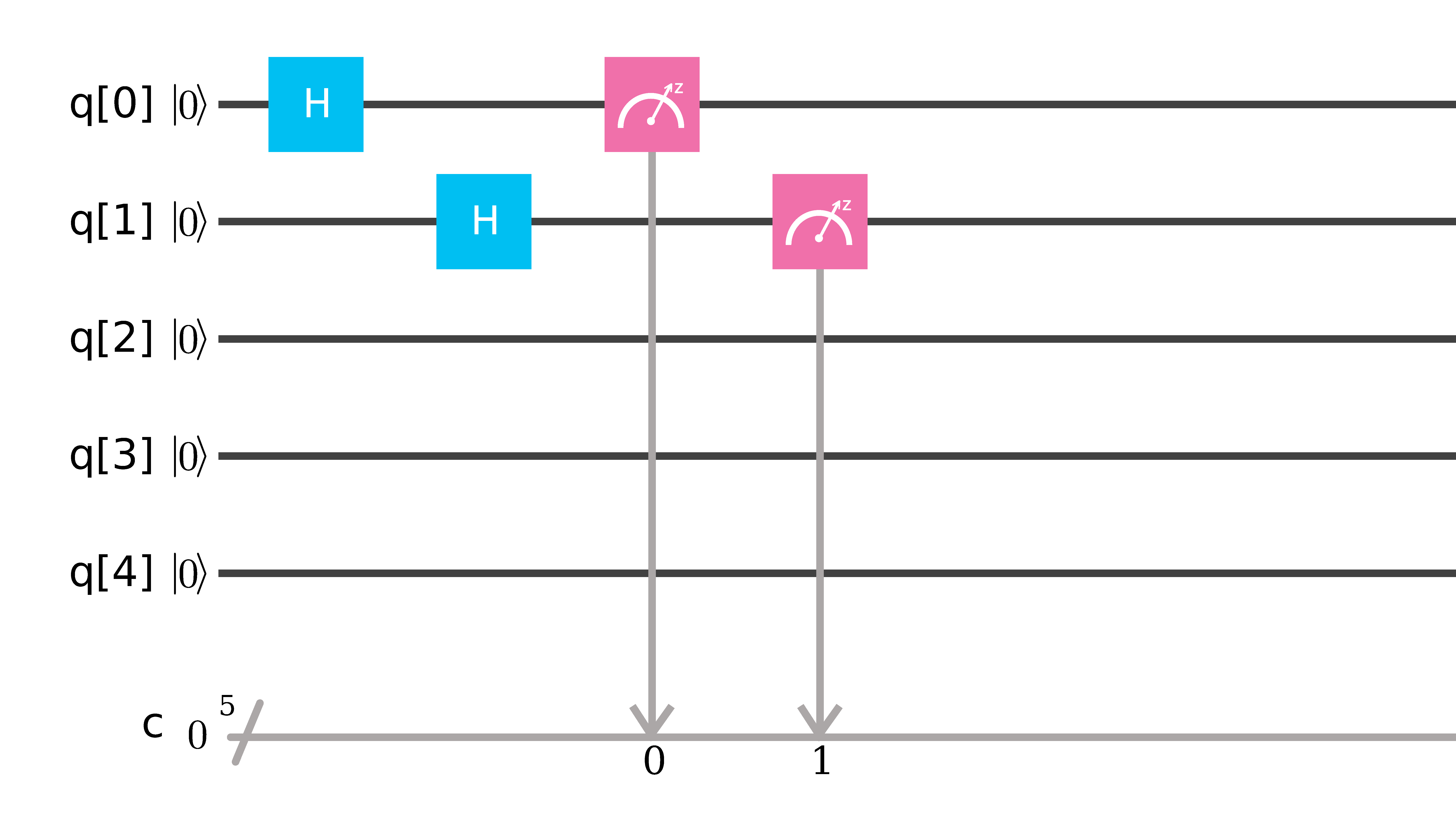
   Figure 2.19: Two-qubit Equal Superposition State

   Solution:
   

   ⬇

   1include ‘‘qelib1.inc’’;

   2qreg q[5];

   3creg c[5];

   4h q[0];

   5h q[1];

   6measure q[0] -> c[0];

   7measure q[1] -> c[1];

   A Hadamard gate transforms the states $\lvert 0\rangle$ and $\lvert 1\rangle$ into $\frac{\lvert 0\rangle+\lvert 1\rangle}{\sqrt{2}}$ and $\frac{\lvert 0\rangle-\lvert 1\rangle}{\sqrt{2}}$ respectively. By applying a Hadamard gate on each qubit, we have just created the equal superposition two-qubit state $\frac{\lvert 0\rangle\lvert 0\rangle+\lvert 0\rangle\lvert 1\rangle+\lvert 1\rangle\lvert 0\rangle+\lvert 1\rangle\lvert 1\rangle}{2}$.

4. Three-qubit Equal Superposition State; Write a QASM code that generates the equal superposition state for three-qubits. To do this:

   • Apply a Hadamard gate in the first qubit

   • Apply a Hadamard gate in the second qubit

   • Apply a Hadamard gate in the third qubit

   • Save the measurement’s result of the first qubit in the first bit

   • Save the measurement’s result of the second qubit in the second bit

   • Save the measurement’s result of the third qubit in the third bit

   

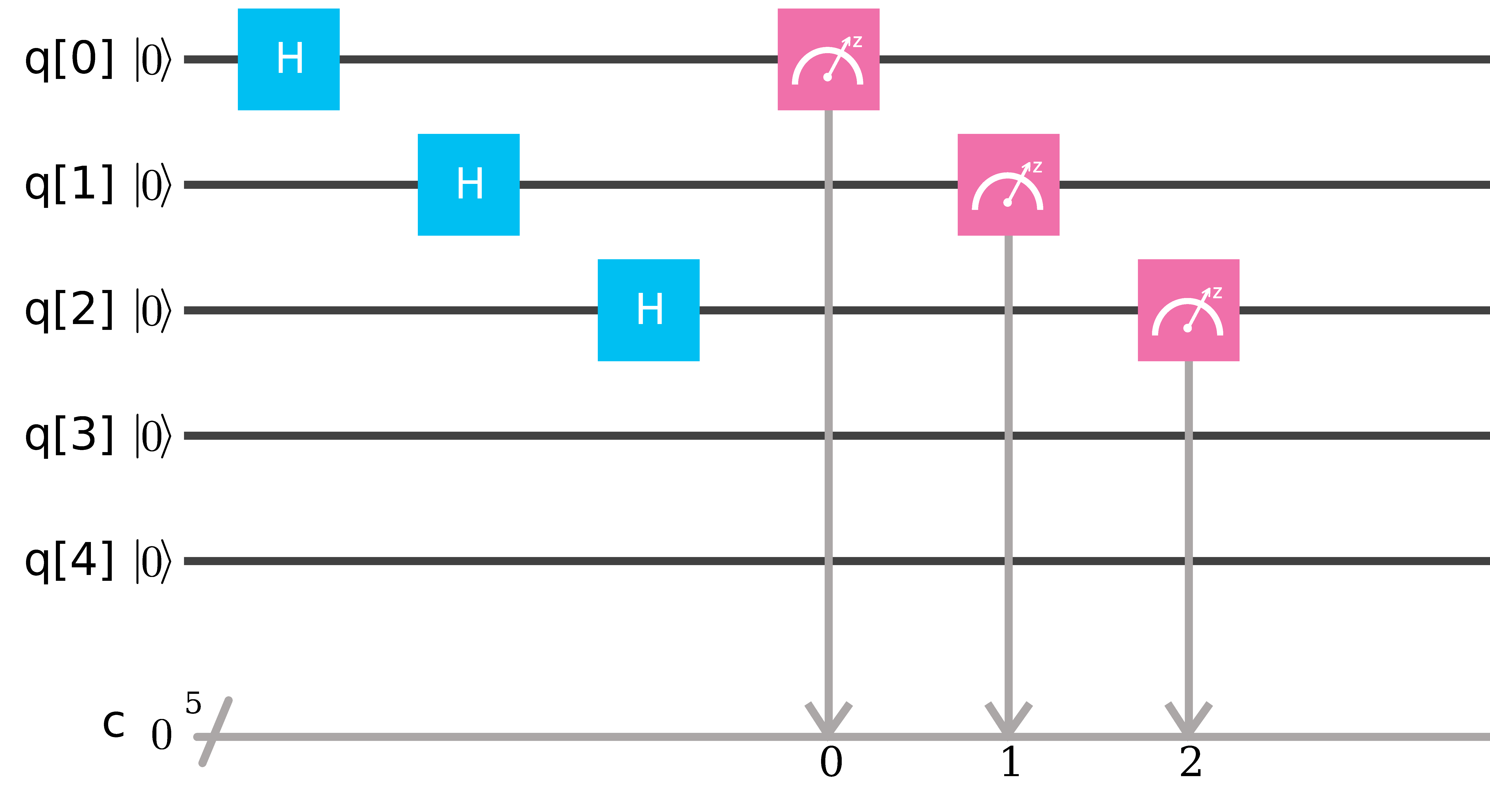
   Figure 2.20: Three-qubit Equal Superposition State

   Solution:
   

   ⬇

   1include ‘‘qelib1.inc’’;

   2qreg q[5];

   3creg c[5];

   4h q[0];

   5h q[1];

   6h q[2];

   7measure q[0] -> c[0];

   8measure q[1] -> c[1];

   9measure q[2] -> c[2];

   2.49   Grover’s Algorithm: Oracle O

   Oracle operation:
   The role of the oracle, O, is to encode the function f(x) in the quantum system and mark the solution. The operation transforms each state of the computational basis as

   $$\left|x\right\rangle\to\left(-1\right)^{f\left(x\right)}\left|x\right\rangle.$$ (2.140)

   In the first iteration of the protocol, this operation transforms the equal superposition state according to:

   $$O\left|\psi\right\rangle\displaystyle=\displaystyle\cos\left(\frac{\theta}{2}\right)O\left|\alpha\right\rangle+\sin\left(\frac{\theta}{2}\right)O\left|\beta\right\rangle\displaystyle=\displaystyle\cos\left(\frac{\theta}{2}\right)\left|\alpha\right\rangle-\sin\left(\frac{\theta}{2}\right)\left|\beta\right\rangle.$$ (2.141)

   The figure below shows the graphical representation of the equal superposition state after the Oracle operator, $O\left|\psi\right\rangle.$ The amplitude of $\left|\psi\right\rangle$ in front of $\left|\alpha\right\rangle$ remains the same as before. However, the amplitude in front of $\left|\beta\right\rangle$ acquires a negative sign. The oracle operation serves to reflect the state $\left|\psi\right\rangle$ about the non-solution state $\left|\alpha\right\rangle$.

   

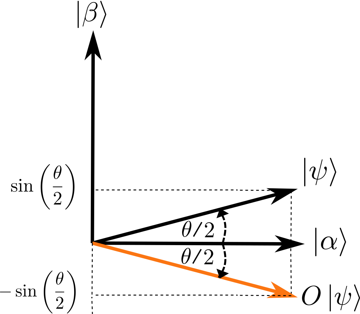
   Figure 2.21: Oracle N

   N=4 item list
   Example 1: If the marked item is $\beta=3$(decimal representation), then the function f is given by $f\left(x\right)=\left\{\begin{array}[]{cc}1,&\text{if }x=11,\\ 0,&\text{otherwise,}\end{array}\right.$

   and therefore the oracle O must transform according to:

   $$\left|\psi\right\rangle\rightarrow\cos\left(30^{\circ}\right)\left|\alpha\right\rangle-\sin\left(30^{\circ}\right)\left|\beta\right\rangle,$$ (2.142)

   where the non-solution state is

   $$\left|\alpha\right\rangle=\frac{1}{\sqrt{3}}\left(\left|0\right\rangle\left|0\right\rangle+\left|0\right\rangle\left|1\right\rangle+\left|1\right\rangle\left|0\right\rangle\right),$$ (2.143)

   and the solution state is

   $$\left|\beta\right\rangle=\left|1\right\rangle\left|1\right\rangle.$$ (2.144)

   In particular, the Oracle must transform each element of the two-qubit basis according to:

   $$\left|0\right\rangle\left|0\right\rangle\displaystyle\rightarrow\displaystyle\left(-1\right)^{f\left(00\right)}\left|0\right\rangle\left|0\right\rangle=\left|0\right\rangle\left|0\right\rangle,$$ (2.145)

   $$\left|0\right\rangle\left|1\right\rangle\displaystyle\rightarrow\displaystyle\left(-1\right)^{f\left(01\right)}\left|0\right\rangle\left|1\right\rangle=\left|0\right\rangle\left|1\right\rangle,$$ (2.146)

   $$\left|1\right\rangle\left|0\right\rangle\displaystyle\rightarrow\displaystyle\left(-1\right)^{f\left(10\right)}\left|1\right\rangle\left|0\right\rangle=\left|1\right\rangle\left|0\right\rangle,$$ (2.147)

   $$\left|1\right\rangle\left|1\right\rangle\displaystyle\rightarrow\displaystyle\left(-1\right)^{f\left(11\right)}\left|1\right\rangle\left|1\right\rangle=-\left|1\right\rangle\left|1\right\rangle.$$ (2.148)

   The figure below shows a graphical representation of the non-solution, solution, and reflected states.

   

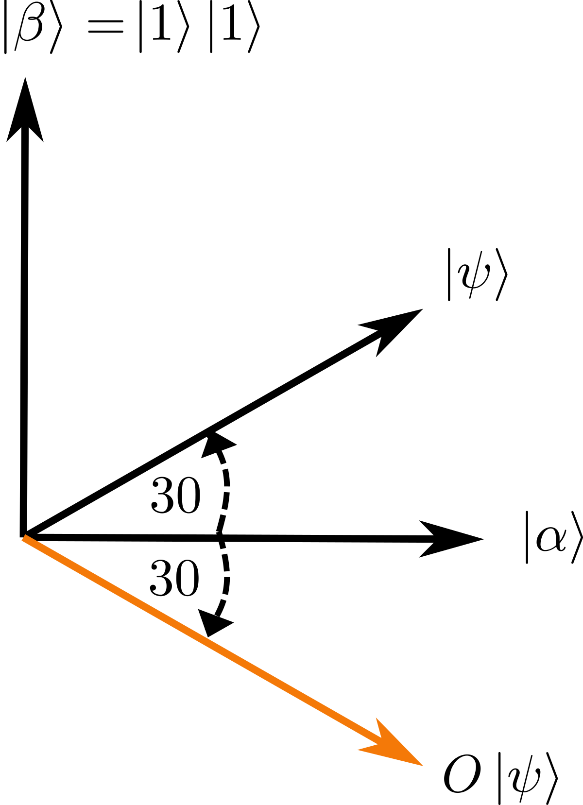
   Figure 2.22: Oracle 2

   The quantum circuit below implements the Oracle for this marked item. We can verify this by computing the state of each element of the basis after the operation. In this case, the Oracle is composed of two Hadamard gates on the second qubit, and one CNOT gate with the first qubit as control and the second as the target. Remember that the Hadamard gate maps a single qubit state according to:

   $$\begin{split}\displaystyle\left|0\right\rangle&\displaystyle\rightarrow\displaystyle\frac{\left|0\right\rangle+\left|1\right\rangle}{\sqrt{2}},\\ \displaystyle\left|1\right\rangle&\displaystyle\rightarrow\displaystyle\frac{\left|0\right\rangle-\left|1\right\rangle}{\sqrt{2}}.\end{split}$$ (2.149)

   And, the CNOT gate maps a two-qubit state according to:

   $$\left|0\right\rangle\left|0\right\rangle\displaystyle\rightarrow\displaystyle\left|0\right\rangle\left|0\right\rangle,$$ (2.150)

   $$\left|0\right\rangle\left|1\right\rangle\displaystyle\rightarrow\displaystyle\left|0\right\rangle\left|1\right\rangle,$$ (2.151)

   $$\left|1\right\rangle\left|0\right\rangle\displaystyle\rightarrow\displaystyle\left|1\right\rangle\left|1\right\rangle,$$ (2.152)

   $$\left|1\right\rangle\left|1\right\rangle\displaystyle\rightarrow\displaystyle\left|1\right\rangle\left|0\right\rangle.$$ (2.153)

   

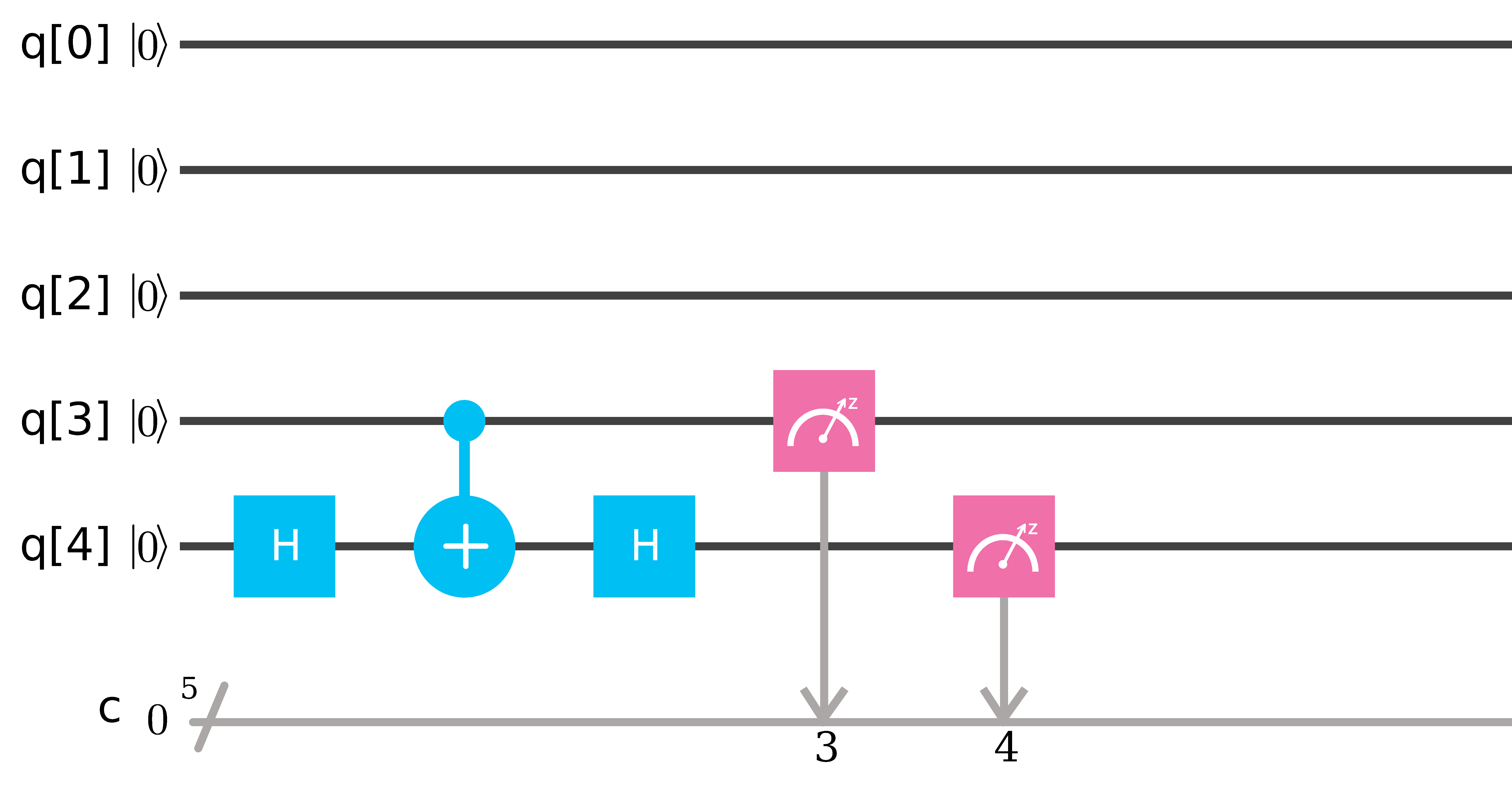
   Figure 2.23: Oracle 11

   The table below shows the evolution of the two-qubit basis states. we can see that the only basis state that acquires a negative sign is the solution state.

   Table 2.8: two-qubit basis states

   Basis State	After first Hadamard H	After CNOT gate	After second Hadamard H
   $\left|0\right\rangle\left|0\right\rangle$	$\left|0\right\rangle\frac{\left|0\right\rangle+\left|1\right\rangle}{\sqrt{2}}$	$\left|0\right\rangle\frac{\left|0\right\rangle+\left|1\right\rangle}{\sqrt{2}}$	$\left|0\right\rangle\left|0\right\rangle$
   $\left|0\right\rangle\left|1\right\rangle$	$\left|0\right\rangle\frac{\left|0\right\rangle-\left|1\right\rangle}{\sqrt{2}}$	$\left|0\right\rangle\frac{\left|0\right\rangle-\left|1\right\rangle}{\sqrt{2}}$	$\left|0\right\rangle\left|1\right\rangle$
   $\left|1\right\rangle\left|0\right\rangle$	$\left|1\right\rangle\frac{\left|0\right\rangle+\left|1\right\rangle}{\sqrt{2}}$	$\left|1\right\rangle\frac{\left|0\right\rangle+\left|1\right\rangle}{\sqrt{2}}$	$\left|1\right\rangle\left|0\right\rangle$
   $\left|1\right\rangle\left|1\right\rangle$	$\left|1\right\rangle\frac{\left|0\right\rangle-\left|1\right\rangle}{\sqrt{2}}$	$-\left|1\right\rangle\frac{\left|0\right\rangle-\left|1\right\rangle}{\sqrt{2}}$	$-\left|1\right\rangle\left|1\right\rangle$

5. N=4: Oracle Operator $\beta=3$; For a list of N=4 items, write the QASM code that generates the Oracle operator when the marked item is $\beta=3$(decimal representation). Use qubits q[3] and q[4] as the first and second qubit respectively. Remember that we are using the ibmqx4 backend [241], and do not forget to measure our two qubits. Compare our results with the table above using $q[3],q[4]=\lvert 0\rangle\lvert 0\rangle.$

   

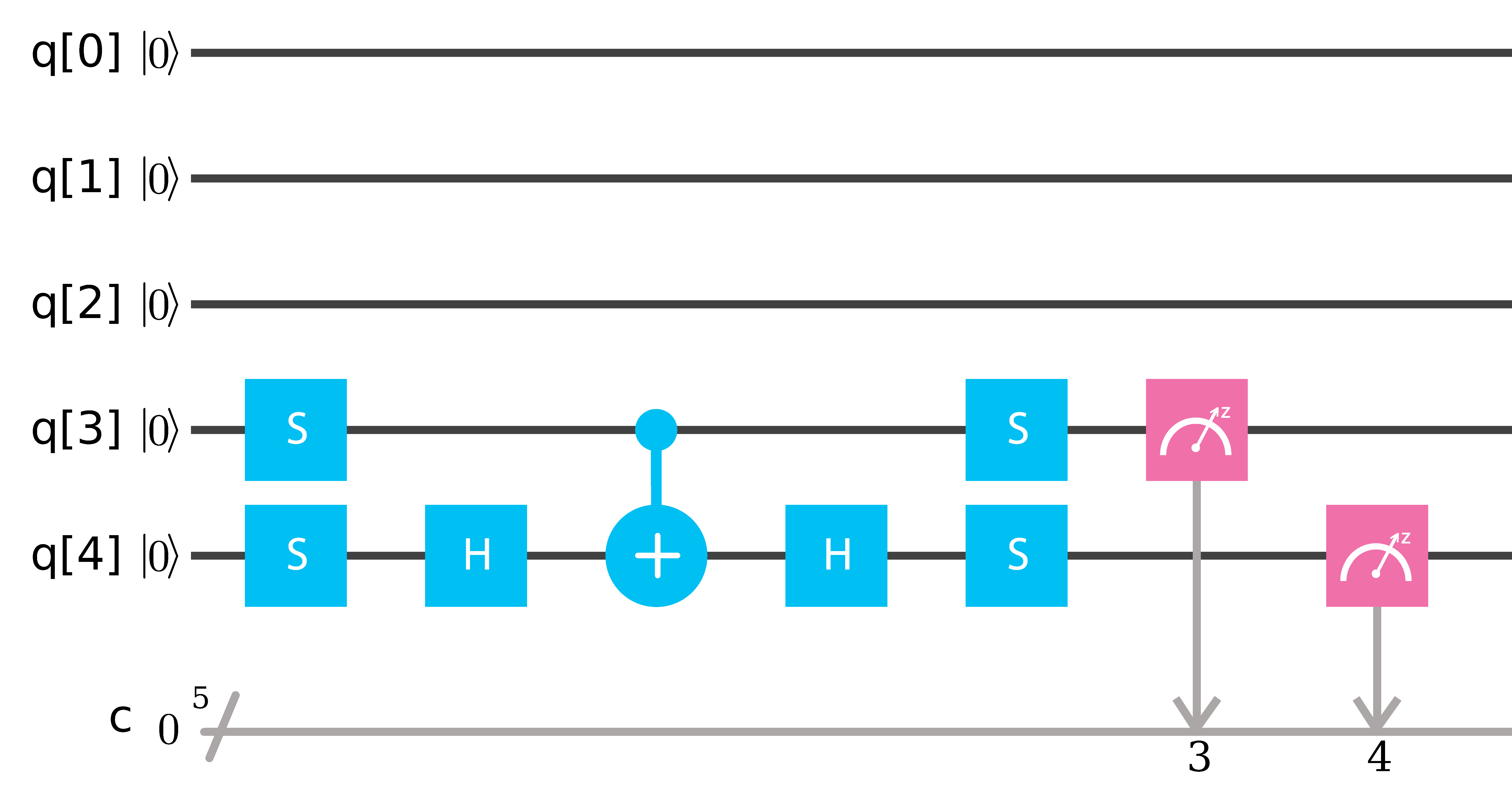
   Figure 2.24: N=4: Oracle Operator $\beta=3$

   Solution:
   

   ⬇

   1 include ‘‘qelib1.inc’’;

   2 qreg q[5];

   3 creg c[5];

   4 h q[4];

   5 cx q[3],q[4];

   6 h q[4];

   7 measure q[3] -> c[3];

   8 measure q[4] -> c[4];

   Example 2: If the marked item is $\beta=2$ (decimal representation), then the function f is given by

   $$f\left(x\right)=\left\{\begin{array}[]{cc}1,&\text{if }x=10,\\ 0,&\text{otherwise.}\end{array}\right.$$ (2.154)

   The Oracle must transform each element of the two-qubit basis according to:

   $\displaystyle\left|0\right\rangle\left|0\right\rangle\displaystyle\rightarrow\displaystyle\left(-1\right)^{f\left(00\right)}\left|0\right\rangle\left|0\right\rangle=\left|0\right\rangle\left|0\right\rangle$

   $\displaystyle\left|0\right\rangle\left|1\right\rangle\displaystyle\rightarrow\displaystyle\left(-1\right)^{f\left(01\right)}\left|0\right\rangle\left|1\right\rangle=\left|0\right\rangle\left|1\right\rangle$

   $\displaystyle\left|1\right\rangle\left|0\right\rangle\displaystyle\rightarrow\displaystyle\left(-1\right)^{f\left(10\right)}\left|1\right\rangle\left|0\right\rangle=-\left|1\right\rangle\left|0\right\rangle$

   $\displaystyle\left|1\right\rangle\left|1\right\rangle\displaystyle\rightarrow\displaystyle\left(-1\right)^{f\left(11\right)}\left|1\right\rangle\left|1\right\rangle=\left|1\right\rangle\left|1\right\rangle$

   

   Figure 2.25: Oracle 10

   The circuit above implements the Oracle for the item $\beta=10$, where the S gate transforms according to:

   $\displaystyle\left|0\right\rangle\displaystyle\rightarrow\displaystyle\left|0\right\rangle$

   $\displaystyle\left|1\right\rangle\displaystyle\rightarrow\displaystyle i\left|1\right\rangle$

   The table below shows the evolution of the basis state under the Oracle. we can see that the only basis state that acquires a negative sign is the solution state $\left|1\right\rangle\left|0\right\rangle$

   Table 2.9: basis state under the Oracle

   Basis State	After first S	After first H	After CNOT	After second H	After second S
   $\left|0\right\rangle\left|0\right\rangle$	$\left|0\right\rangle\left|0\right\rangle$	$\left|0\right\rangle\frac{\left|0\right\rangle+\left|1\right\rangle}{\sqrt{2}}$	$\left|0\right\rangle\frac{\left|0\right\rangle+\left|1\right\rangle}{\sqrt{2}}$	$\left|0\right\rangle\left|0\right\rangle$	$\left|0\right\rangle\left|0\right\rangle$
   $\left|0\right\rangle\left|1\right\rangle$	$\left|0\right\rangle\left|1\right\rangle$	$\left|0\right\rangle\frac{\left|0\right\rangle-\left|1\right\rangle}{\sqrt{2}}$	$\left|0\right\rangle\frac{\left|0\right\rangle-\left|1\right\rangle}{\sqrt{2}}$	$\left|0\right\rangle\left|1\right\rangle$	$\left|0\right\rangle\left|1\right\rangle$
   $\left|1\right\rangle\left|0\right\rangle$	$i\left|1\right\rangle\left|0\right\rangle$	$i\left|1\right\rangle\frac{\left|0\right\rangle+\left|1\right\rangle}{\sqrt{2}}$	$i\left|1\right\rangle\frac{\left|0\right\rangle+\left|1\right\rangle}{\sqrt{2}}$	$i\left|1\right\rangle\left|0\right\rangle$	$-\left|1\right\rangle\left|0\right\rangle$
   $\left|1\right\rangle\left|1\right\rangle$	$i\left|1\right\rangle\left|1\right\rangle$	$i\left|1\right\rangle\frac{\left|0\right\rangle-\left|1\right\rangle}{\sqrt{2}}$	$-i\left|1\right\rangle\frac{\left|0\right\rangle-\left|1\right\rangle}{\sqrt{2}}$	$-i\left|1\right\rangle\left|1\right\rangle$	$\left|1\right\rangle\left|1\right\rangle$

6. N=4: Oracle Operator $\beta=2$; For a list of N=4 items, write the QASM code [233] that generates the Oracle operator when the marked item is $\beta=2$(decimal representation). Use qubits q[3] and q[4] as the first and second qubit respectively.

   

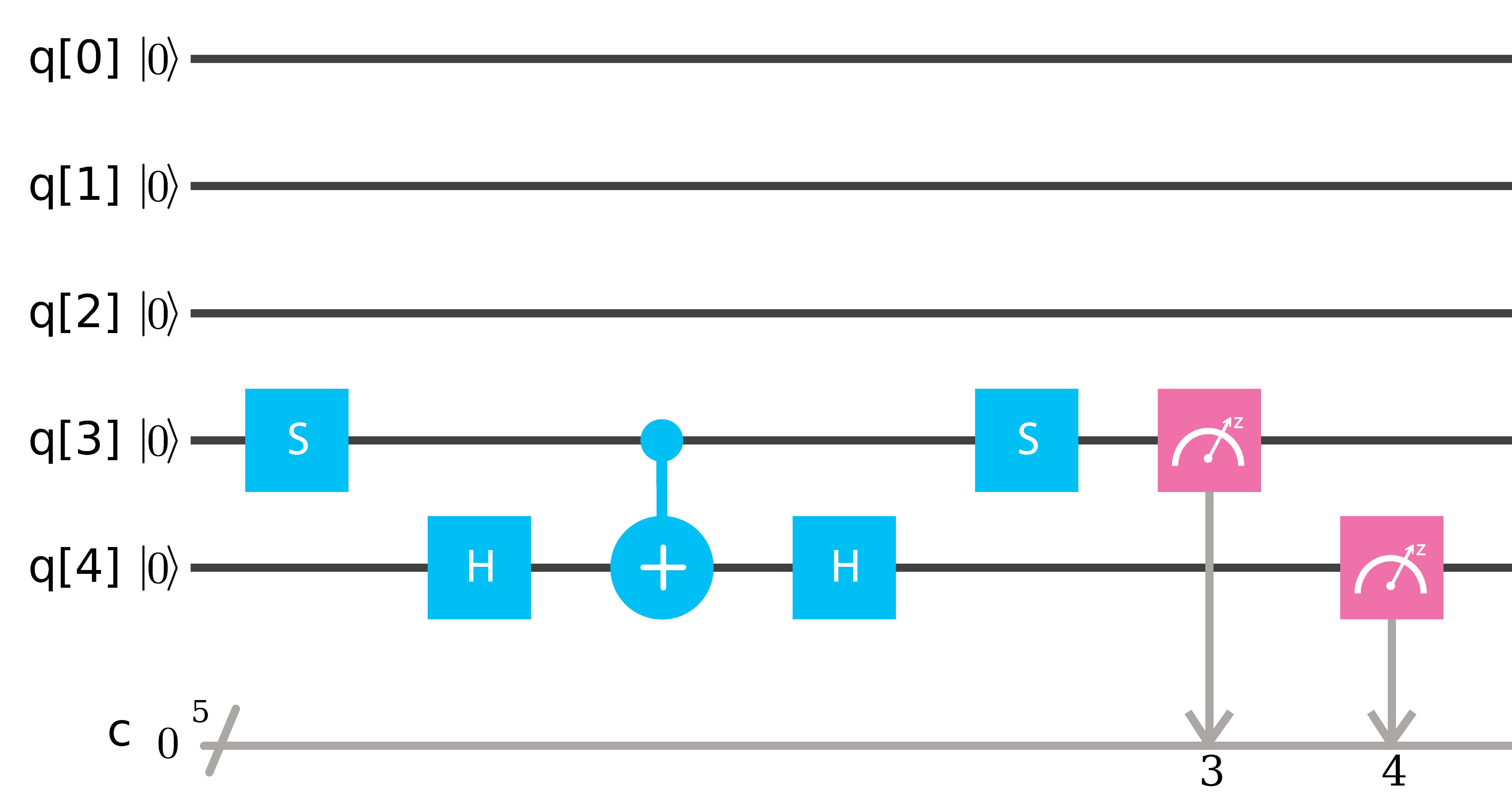
   Figure 2.26: N=4: Oracle Operator $\beta=2$

   Solution:
   

   ⬇

   1 include ‘‘qelib1.inc’’;

   2 qreg q[5];

   3 creg c[5];

   4 s q[3];

   5 h q[4];

   6 cx q[3],q[4];

   7 h q[4];

   8 s q[3];

   9 measure q[3] -> c[3];

   10 measure q[4] -> c[4];

   2.50   Grover’s Algorithm: Grover Operator

   Reflection W:
   The third step in Grover’s algorithm is given by the implementation of the second reflection, which we will call W. Let us recall the state after the first implementation of the Oracle Operator,

   $$O\left|\psi\right\rangle=\cos\left(\frac{\theta}{2}\right)\left|\alpha\right\rangle-\sin\left(\frac{\theta}{2}\right)\left|\beta\right\rangle.$$ (2.155)

   The $\beta$operator then corresponds to a reflection about the equal superposition state $\left|\psi\right\rangle$. Since this operator does not depend on the function f(x) and, rather, depends only on the superposition state, W is the same for any marked item $\beta$.

   Grover Operator
   We define the Grover operator as $G=WO,$

   that is, the application of the Oracle operator followed by the W reflection.

   $$G\left|\psi\right\rangle=\cos\left(\frac{3\theta}{2}\right)\left|\alpha\right\rangle+\sin\left(\frac{3\theta}{2}\right)\left|\beta\right\rangle$$ (2.156)

   

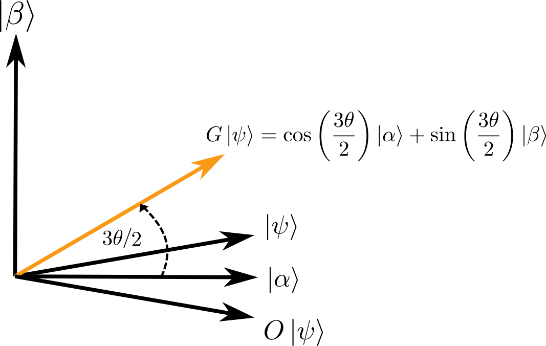
   Figure 2.27: N Grover

   The state after the second Grover iteration is:

   $$G^{2}\left|\psi\right\rangle=\cos\left(\frac{5\theta}{2}\right)\left|\alpha\right\rangle+\sin\left(\frac{5\theta}{2}\right)\left|\beta\right\rangle$$ (2.157)

   

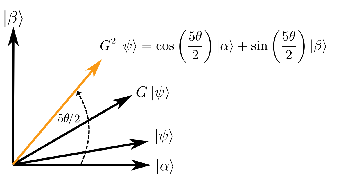
   Figure 2.28: N Grover

   In general, the state after the k-th Grover iteration will be given by

   $$G^{k}\left|\psi\right\rangle=\cos\left(\frac{2k+1}{2}\theta\right)\left|\alpha\right\rangle+\sin\left(\frac{2k+1}{2}\theta\right)\left|\beta\right\rangle$$ (2.158)

   $N=4$ items: Marked item $\beta=11$
   

   As we discussed in the previous section, the equal superposition state for a list of 4 items is given by:

   $$\left|\psi\right\rangle=\cos\left(30^{\circ}\right)\left|\alpha\right\rangle+\sin\left(30^{\circ}\right)\left|\beta\right\rangle,$$ (2.159)

   where the non-solution and solution states are respectively given by

   $$\begin{split}\displaystyle\left|\alpha\right\rangle\displaystyle&=\displaystyle\frac{\left|0\right\rangle\left|0\right\rangle+\left|0\right\rangle\left|1\right\rangle+\left|1\right\rangle\left|0\right\rangle}{\sqrt{3}},\\ \displaystyle\left|\beta\right\rangle\displaystyle&=\displaystyle\left|1\right\rangle\left|1\right\rangle\end{split}$$ (2.160)

   After the Oracle operator for the item $\beta=11$ is applied, the equal superposition state $\lvert\psi\rangle$is reflected about the non-solution state $\lvert\alpha\rangle$

   $$O\left|\psi\right\rangle=\cos\left(30^{\circ}\right)\left|\alpha\right\rangle-\sin\left(30^{\circ}\right)\left|\beta\right\rangle.$$ (2.161)

   The second reflection is applied, and this reflects the state $O\left|\psi\right\rangle$ about the equal superposition state $\left|\psi\right\rangle$,

   $$WO\left|\psi\right\rangle=\cos\left(90^{\circ}\right)\left|\alpha\right\rangle+\sin\left(90^{\circ}\right)\left|\beta\right\rangle.$$ (2.162)

   How many times should we apply the Grover Operator? For a list of $N=4$ items and one marked item $\beta$, the number of necessary repetitions R required to find w is bounded above by:

   $$\begin{split}\displaystyle R&\displaystyle\leq\displaystyle\frac{\pi}{4}\sqrt{4},\\ &\displaystyle\leq\displaystyle\frac{\pi}{4}\sqrt{4},\\ &\displaystyle\leq\displaystyle 1.5\end{split}$$ (2.163)

   Since the upper bound is $\approx 1.5$, we know that the optimal number of iterations to find the marked item is equal to one. The state after the first Grover iteration, $G=WO$, is given by

   $$G\left|\psi\right\rangle=\cos\left(90^{\circ}\right)\left|\alpha\right\rangle+\sin\left(90^{\circ}\right)\left|\beta\right\rangle.$$ (2.164)

   The figure below illustrates the final state after the first Grover iteration. we can see that the final state matches the solution state.

   

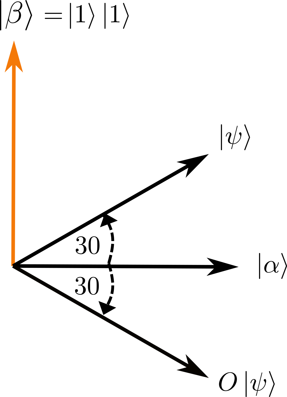
   Figure 2.29: N4 Grover

   From the figure below, we can see that applying the Grover operator a second time, $G^{2}=\left(WO\right)^{2}$, does not improve the performance of the algorithm. After a second iteration, the resulting state moves away from the solution state,

   $$G^{2}\left|\psi\right\rangle=\cos\left(150\right)\left|\alpha\right\rangle+\sin\left(150\right)\left|\beta\right\rangle$$ (2.165)

   

   Figure 2.30: N4 Grover

7. W Reflection for N=4 items; The figure below shows the quantum circuit used to implement the reflection W for a list of N=4 items. Write the QASM code that generates this quantum circuit.

   

   Figure 2.31: Reflection N4

   Solution:
   

   ⬇

   1 include ‘‘qelib1.inc’’;

   2 qreg q[5];

   3 creg c[5];

   4 h q[3];

   5 h q[4];

   6 x q[3];

   7 x q[4];

   8 h q[4];

   9 cx q[3],q[4];

   10 h q[4];

   11 x q[3];

   12 x q[4];

   13 h q[3];

   14 h q[4];

   15 measure q[3] -> c[3];

   16 measure q[4] -> c[4];

   2.51   Grover’s Algorithm: Putting it All Together

   By now, we have seen how to implement each step of Grover’s algorithm: Initialization, Oracle $O$, and Reflection W, where the last two correspond to the implementation of the Grover operator $G=WO$. In particular, we discussed the compiled quantum circuit to implement the Oracles for two marked items in a list of $N=4$ items. In this section of the IBM Q experience, we will program Grover’s algorithm for all the possible marked items when $N=4$.

8. Grover’s Algorithm: N=4 Items with $\beta=00$; The figure below shows the quantum circuit to implement Grover’s algorithm for a list of N=4 items with $\beta=00$. Write the QASM code that generates this quantum circuit.

   

   Figure 2.32: Grover final

   Solution:
   

   ⬇

   1 include ‘‘qelib1.inc’’;

   2 qreg q[5];

   3 creg c[5];

   4 //INITIALIZATION

   5 h q[3];

   6 h q[4];

   7 //ORACLE 00

   8 s q[3];

   9 s q[4];

   10 h q[4];

   11 cx q[3],q[4];

   12 h q[4];

   13 s q[3];

   14 s q[4];

   15 //REFLECTION

   16 h q[3];

   17 h q[4];

   18 x q[3];

   19 x q[4];

   20 h q[4];

   21 cx q[3],q[4];

   22 h q[4];

   23 x q[3];

   24 x q[4];

   25 h q[3];

   26 h q[4];

   27 measure q[3] -> c[3];

   28 measure q[4] -> c[4];

   In this circuit, the first two Hadamard gates, H, create the equal superposition two-qubit state

   $\frac{\left|0\right\rangle\left|0\right\rangle+\left|0\right\rangle\left|1\right\rangle+\left|1\right\rangle\left|0\right\rangle+\left|1\right\rangle\left|1\right\rangle}{2}$

   The following combination of four S gates, two H gates, and one CNOT gate implements the oracle O for the marked item $\beta=00$ in binary notation. This oracle leaves the two-qubit system in

   $\frac{-\left|0\right\rangle\left|0\right\rangle+\left|0\right\rangle\left|1\right\rangle+\left|1\right\rangle\left|0\right\rangle+\left|1\right\rangle\left|1\right\rangle}{2}$

   The remaining section of the circuit implements the reflection W for a two-qubit system. The Grover operator $G=WO$ maps the equal superpostition state as

   $\frac{\left|0\right\rangle\left|0\right\rangle+\left|0\right\rangle\left|1\right\rangle+\left|1\right\rangle\left|0\right\rangle+\left|1\right\rangle\left|1\right\rangle}{2}\rightarrow\left|0\right\rangle\left|0\right\rangle$

   we can see that the analytical result agrees with the simulation. The higher frequency is given by the measurement result $(c_{4},c_{3},c_{2},c_{1},c_{0})=(0,0,0,0,0)$, where$c_{0},c_{1},c_{2},c_{3}$, and $c_{4}$ refers to the measurement result of qubit $q_{0},q_{1},q_{2},q_{3},$ and $q_{4}$ respectively.

9. Grover’s Algorithm: N=4 Items with $\beta=01$; The figure below shows the quantum circuit to implement Grover’s algorithm for a list of N=4 items with $\beta=01$. Write the QASM code that generates this quantum circuit.

   

   Figure 2.33: Grover final

   Solution:
   

   ⬇

   1 include ‘‘qelib1.inc’’;

   2 qreg q[5];

   3 creg c[5];

   4 //INITIALIZATION

   5 h q[4];

   6 //ORACLE 01

   7 s q[4];

   8 h q[4];

   9 cx q[3],q[4];

   10 h q[4];

   11 s q[4];

   12 //REFLECTION

   13 h q[3];

   14 h q[4];

   15 x q[3];

   16 x q[4];

   17 h q[4];

   18 cx q[3],q[4];

   19 h q[4];

   20 x q[3];

   21 x q[4];

   22 h q[3];

   23 h q[4];

   24 measure q[3] -> c[3];

   25 measure q[4] -> c[4];

   In this circuit, the first two Hadamard gates, H, create the equal superposition two-qubit state

   $\frac{\left|0\right\rangle\left|0\right\rangle+\left|0\right\rangle\left|1\right\rangle+\left|1\right\rangle\left|0\right\rangle+\left|1\right\rangle\left|1\right\rangle}{2}$

   The following combination of two S gates, two H gates, and one CNOT gate implements the oracle O for the marked item $\beta=01$ in binary notation. This oracle leaves the two-qubit system in

   $\frac{\left|0\right\rangle\left|0\right\rangle-\left|0\right\rangle\left|1\right\rangle+\left|1\right\rangle\left|0\right\rangle+\left|1\right\rangle\left|1\right\rangle}{2}$

   The remaining section of the circuit implements the reflection W for a two-qubit system. The Grover operator $G=WO$ maps the equal superpostition state as

   $\frac{\left|0\right\rangle\left|0\right\rangle+\left|0\right\rangle\left|1\right\rangle+\left|1\right\rangle\left|0\right\rangle+\left|1\right\rangle\left|1\right\rangle}{2}\rightarrow\left|0\right\rangle\left|1\right\rangle$

   we can see that the analytical result agrees with the simulation. The higher frequency is given by the measurement result $(c_{4},c_{3},c_{2},c_{1},c_{0})=(1,0,0,0,0)$, where$c_{0},c_{1},c_{2},c_{3}$, and $c_{4}$ refers to the measurement result of qubit $q_{0},q_{1},q_{2},q_{3},$ and $q_{4}$ respectively.

10. The figure below shows the quantum circuit to implement Grover’s algorithm for a list of N=4 items with $\beta=10$. Write the QASM code that generates this quantum circuit.

    

    Figure 2.34: Grover final

    Solution:
    

    ⬇

    1 include ‘‘qelib1.inc’’;

    2 qreg q[5];

    3 creg c[5];

    4 //INITIALIZATION

    5 h q[3];

    6 h q[4];

    7 //ORACLE10

    8 s q[3];

    9 h q[4];

    10 cx q[3],q[4];

    11 h q[4];

    12 s q[3];

    13 //REFLECTION

    14 h q[3];

    15 h q[4];

    16 x q[3];

    17 x q[4];

    18 h q[4];

    19 cx q[3],q[4];

    20 h q[4];

    21 x q[3];

    22 x q[4];

    23 h q[3];

    24 h q[4];

    25 measure q[3] -> c[3];

    26 measure q[4] -> c[4];

    In this circuit, the first two Hadamard gates, H, create the equal superposition two-qubit state

    $\frac{\left|0\right\rangle\left|0\right\rangle+\left|0\right\rangle\left|1\right\rangle+\left|1\right\rangle\left|0\right\rangle+\left|1\right\rangle\left|1\right\rangle}{2}$

    The following combination of two S gates, two H gates, and one CNOT gate implements the oracle O for the marked item $\beta=10$ in binary notation. This oracle leaves the two-qubit system in

    $\frac{\left|0\right\rangle\left|0\right\rangle+\left|0\right\rangle\left|1\right\rangle-\left|1\right\rangle\left|0\right\rangle+\left|1\right\rangle\left|1\right\rangle}{2}$

    The remaining section of the circuit implements the reflection W for a two-qubit system. The Grover operator $G=WO$ maps the equal superpostition state as

    $\frac{\left|0\right\rangle\left|0\right\rangle+\left|0\right\rangle\left|1\right\rangle+\left|1\right\rangle\left|0\right\rangle+\left|1\right\rangle\left|1\right\rangle}{2}\rightarrow\left|1\right\rangle\left|0\right\rangle$

    we can see that the analytical result agrees with the simulation. The higher frequency is given by the measurement result $(c_{4},c_{3},c_{2},c_{1},c_{0})=(0,1,0,0,0),$ where $c_{0},c_{1},c_{2},c_{3},$ and $c_{4}$ refers to the measurement result of qubit $q_{0},q_{1},q_{2},q_{3},$ and $q_{4}$ respectively.

11. The figure below shows the quantum circuit to implement Grover’s algorithm for a list of N=4 items with $\beta=11$. Write the QASM code that generates this quantum circuit.

    

    Figure 2.35: Grover final

    Solution:
    

    ⬇

    1 include ‘‘qelib1.inc’’;

    2 qreg q[5];

    3 creg c[5];

    4 //INITIALIZATION

    5 h q[3];

    6 h q[4];

    7 //ORACLE11

    8 h q[4];

    9 cx q[3],q[4];

    10 h q[4];

    11 //REFLECTION

    12 h q[3];

    13 h q[4];

    14 x q[3];

    15 x q[4];

    16 h q[4];

    17 cx q[3],q[4];

    18 h q[4];

    19 x q[3];

    20 x q[4];

    21 h q[3];

    22 h q[4];

    23 measure q[3] -> c[3];

    24 measure q[4] -> c[4];

    In this circuit, the first two Hadamard gates, H, create the equal superposition two-qubit state

    $\frac{\left|0\right\rangle\left|0\right\rangle+\left|0\right\rangle\left|1\right\rangle+\left|1\right\rangle\left|0\right\rangle+\left|1\right\rangle\left|1\right\rangle}{2}$

    The following combination of two H gates, and one CNOT gate implements the oracle O for the marked item $\beta=11$ in binary notation. This oracle leaves the two-qubit system in

    $\frac{\left|0\right\rangle\left|0\right\rangle+\left|0\right\rangle\left|1\right\rangle+\left|1\right\rangle\left|0\right\rangle-\left|1\right\rangle\left|1\right\rangle}{2}$

    The remaining section of the circuit implements the reflection W for a two-qubit system. The Grover operator $G=WO$ maps the equal superpostition state as

    $\frac{\left|0\right\rangle\left|0\right\rangle+\left|0\right\rangle\left|1\right\rangle+\left|1\right\rangle\left|0\right\rangle+\left|1\right\rangle\left|1\right\rangle}{2}\rightarrow\left|1\right\rangle\left|1\right\rangle$

    we can see that the analytical result agrees with the simulation. The higher frequency is given by the measurement result $(c_{4},c_{3},c_{2},c_{1},c_{0})=(1,1,0,0,0),$ where $c_{0},c_{1},c_{2},c_{3},$ and $c_{4}$ refers to the measurement result of qubit $q_{0},q_{1},q_{2},q_{3},$ and $q_{4}$ respectively.

Figure 2.36: Quantum Annealing

Figure 2.37: Grovers Algorithm

Index

Part III Quantum-Computation and Quantum-Communication

CHAPTER 3  Quantum-Computation and Quantum-Communication

References

- [1] M. A. Nielsen and I. L. Chuang, Quantum Computation and Quantum Information: 10th Anniversary Edition, 10th ed. USA: Cambridge University Press, 2011.
- [2] I. Chuang, Quantum Information Science II MIT EECS 6.443J / Physics 8.371J / 18.409, 2014, publication Title: Quantum Information Science II MIT 6.443J / 8.371J / 18.409. [Online]. Available: http://cua.scripts.mit.edu/8.371/S2014/index.php
- [3] J. Preskill, Quantum Computation Physics 219/Computer Science 219 (Formerly Physics 229), 2019, publication Title: Quantum Computation Physics 219/Computer Science 219 (Formerly Physics 229). [Online]. Available: http://www.theory.caltech.edu/preskill/ph219/index.html
- [4] U. Vazirani, Quantum Computation CS294-2, 1997, publication Title: CS294-2 Quantum Computation Fall 1997. [Online]. Available: https://people.eecs.berkeley.edu/vazirani/qc.html
- [5] J. Watrous, Theory of Quantum Information John Watrous’s Lecture Notes, 2011, publication Title: John Watrous’s Lecture Notes Theory of Quantum Information (notes from Fall 2011). [Online]. Available: https://cs.uwaterloo.ca/watrous/LectureNotes.html
- [6] U. Vazirani, Quantum Computation CS294-2, 2007, publication Title: Quantum Computation CS294-2. [Online]. Available: https://people.eecs.berkeley.edu/vazirani/quantum.html
- [7] S. Aaronson, Quantum Computing Since Democritus PHYS771, 2006, publication Title: Quantum Computing Since Democritus PHYS771. [Online]. Available: https://www.scottaaronson.com/democritus/
- [8] P. W. Shor, Quantum Computation, 2003, publication Title: Quantum Computation MIT Course Number 18.435J / 2.111J / ESD.79J. [Online]. Available: https://ocw.mit.edu/courses/mathematics/18-435j-quantum-computation-fall-2003/
- [9] I. Chuang and P. Shor, Quantum Information Science, 2006, publication Title: Quantum Information Science MIT Course Number MAS.865J / 6.443J / 8.371J. [Online]. Available: https://ocw.mit.edu/courses/media-arts-and-sciences/mas-865j-quantum-information-science-spring-2006/
- [10] S. Aaronson, Quantum Complexity Theory, 2010, publication Title: Quantum Complexity Theory MIT Course Number 6.845. [Online]. Available: https://ocw.mit.edu/courses/electrical-engineering-and-computer-science/6-845-quantum-complexity-theory-fall-2010/
- [11] A. W. Harrow, Quantum Information Science 6.443/8.371/18.436, 2018, publication Title: Quantum Information Science 6.443/8.371/18.436. [Online]. Available: https://web.mit.edu/8.371/www/index.html
- [12] A. Childs, Quantum algorithms CO 781, 2008, publication Title: Quantum algorithms (CO 781, Winter 2008) Type: This course will cover recent developments in quantum algorithms. The objectives of the course are to bring graduate students up to speed with the state of the art in quantum algorithms, and to prepare them to work on research problems in quantum computing. The course will be roughly divided into three parts, on the hidden subgroup problem, quantum walk, and adiabatic quantum computation. [Online]. Available: http://www.math.uwaterloo.ca/amchilds/teaching/w08/co781.html
- [13] R. Cleve, Introduction to Quantum Information Processing CS 667, C&O 681, PHYS 767, 2007, publication Title: Introduction to Quantum Information Processing CS 667, C&O 681, PHYS 767 Fall 2007. [Online]. Available: https://cs.uwaterloo.ca/cleve/courses/F07CS667/index.html
- [14] M. Russo, A. Thaker, and S. Adam, The Coming Quantum Leap in Computing, May 2018. [Online]. Available: https://www.bcg.com/en-in/publications/2018/coming-quantum-leap-computing.aspx
- [15] The Next Decade in Quantum Computing—and How to Play. [Online]. Available: https://www.bcg.com/en-in/publications/2018/next-decade-quantum-computing-how-play.aspx
- [16] “Here, there and everywhere,” The Economist. [Online]. Available: https://www.economist.com/news/essays/21717782-quantum-technology-beginning-come-its-own
- [17] A. W. Harrow, “Why now is the right time to study quantum computing,” XRDS: Crossroads, The ACM Magazine for Students, vol. 18, no. 3, pp. 32–37, Mar. 2012. [Online]. Available: http://arxiv.org/abs/1501.00011
- [18] M. Sisodia, A. Shukla, A. A. A. de Almeida, G. W. Dueck, and A. Pathak, “Circuit optimization for IBM processors: A way to get higher fidelity and higher values of nonclassicality witnesses,” arXiv:1812.11602 [quant-ph], Dec. 2018. [Online]. Available: http://arxiv.org/abs/1812.11602
- [19] A. Cervera-Lierta, “Exact Ising model simulation on a quantum computer,” Quantum, vol. 2, p. 114, Dec. 2018. [Online]. Available: http://arxiv.org/abs/1807.07112
- [20] J. R. McClean, K. J. Sung, I. D. Kivlichan, Y. Cao, C. Dai, E. S. Fried, C. Gidney, B. Gimby, P. Gokhale, T. Häner, T. Hardikar, V. Havlíček, O. Higgott, C. Huang, J. Izaac, Z. Jiang, X. Liu, S. McArdle, M. Neeley, T. O’Brien, B. O’Gorman, I. Ozfidan, M. D. Radin, J. Romero, N. Rubin, N. P. D. Sawaya, K. Setia, S. Sim, D. S. Steiger, M. Steudtner, Q. Sun, W. Sun, D. Wang, F. Zhang, and R. Babbush, “OpenFermion: The Electronic Structure Package for Quantum Computers,” arXiv:1710.07629 [physics, physics:quant-ph], Feb. 2019. [Online]. Available: http://arxiv.org/abs/1710.07629
- [21] E. Farhi, J. Goldstone, and S. Gutmann, “A Quantum Approximate Optimization Algorithm,” arXiv:1411.4028 [quant-ph], Nov. 2014. [Online]. Available: http://arxiv.org/abs/1411.4028
- [22] S. E. Smart, D. I. Schuster, and D. A. Mazziotti, “Experimental data from a quantum computer verifies the generalized Pauli exclusion principle,” Communications Physics, vol. 2, no. 1, pp. 1–6, Jan. 2019. [Online]. Available: https://www.nature.com/articles/s42005-019-0110-3
- [23] N. N. Hegade, B. K. Behera, and P. K. Panigrahi, “Experimental Demonstration of Quantum Tunneling in IBM Quantum Computer,” arXiv:1712.07326 [quant-ph], Feb. 2019. [Online]. Available: http://arxiv.org/abs/1712.07326
- [24] M. J. Bremner, R. Jozsa, and D. J. Shepherd, “Classical simulation of commuting quantum computations implies collapse of the polynomial hierarchy,” Proceedings of the Royal Society A: Mathematical, Physical and Engineering Sciences, vol. 467, no. 2126, pp. 459–472, Feb. 2011. [Online]. Available: http://arxiv.org/abs/1005.1407
- [25] T. Shang, K. Li, R. Chen, and J. Liu, “Continuous-Variable Quantum Network Coding Against Pollution Attacks,” in Quantum Technology and Optimization Problems, ser. Lecture Notes in Computer Science, S. Feld and C. Linnhoff-Popien, Eds. Cham: Springer International Publishing, 2019, pp. 196–206.
- [26] S.-K. Liao, W.-Q. Cai, J. Handsteiner, B. Liu, J. Yin, L. Zhang, D. Rauch, M. Fink, J.-G. Ren, W.-Y. Liu, Y. Li, Q. Shen, Y. Cao, F.-Z. Li, J.-F. Wang, Y.-M. Huang, L. Deng, T. Xi, L. Ma, T. Hu, L. Li, N.-L. Liu, F. Koidl, P. Wang, Y.-A. Chen, X.-B. Wang, M. Steindorfer, G. Kirchner, C.-Y. Lu, R. Shu, R. Ursin, T. Scheidl, C.-Z. Peng, J.-Y. Wang, A. Zeilinger, and J.-W. Pan, “Satellite-Relayed Intercontinental Quantum Network,” Physical Review Letters, vol. 120, no. 3, p. 030501, Jan. 2018. [Online]. Available: https://link.aps.org/doi/10.1103/PhysRevLett.120.030501
- [27] C. L. Edmunds, C. Hempel, R. Harris, H. Ball, V. Frey, T. M. Stace, and M. J. Biercuk, “Measuring and Suppressing Error Correlations in Quantum Circuits,” arXiv:1712.04954 [quant-ph], Dec. 2017. [Online]. Available: http://arxiv.org/abs/1712.04954
- [28] J. Preskill, “Quantum Computing in the NISQ era and beyond,” Quantum, vol. 2, p. 79, Aug. 2018. [Online]. Available: http://arxiv.org/abs/1801.00862
- [29] M. Delehaye and C. Lacroûte, “Single-ion, transportable optical atomic clocks,” Journal of Modern Optics, vol. 65, no. 5-6, pp. 622–639, Mar. 2018. [Online]. Available: http://arxiv.org/abs/1804.02168
- [30] N. Huntemann, C. Sanner, B. Lipphardt, C. Tamm, and E. Peik, “Single-ion atomic clock with $3\textbackslashtimes 10ˆ-18$ systematic uncertainty,” Physical Review Letters, vol. 116, no. 6, p. 063001, Feb. 2016. [Online]. Available: https://link.aps.org/doi/10.1103/PhysRevLett.116.063001
- [31] R. LaRose, “Overview and Comparison of Gate Level Quantum Software Platforms,” Quantum, vol. 3, p. 130, Mar. 2019. [Online]. Available: http://arxiv.org/abs/1807.02500
- [32] N. Killoran, J. Izaac, N. Quesada, V. Bergholm, M. Amy, and C. Weedbrook, “Strawberry Fields: A Software Platform for Photonic Quantum Computing,” Quantum, vol. 3, p. 129, Mar. 2019. [Online]. Available: http://arxiv.org/abs/1804.03159
- [33] A. D. King, J. Carrasquilla, J. Raymond, I. Ozfidan, E. Andriyash, A. Berkley, M. Reis, T. Lanting, R. Harris, F. Altomare, K. Boothby, P. I. Bunyk, C. Enderud, A. Fréchette, E. Hoskinson, N. Ladizinsky, T. Oh, G. Poulin-Lamarre, C. Rich, Y. Sato, A. Y. Smirnov, L. J. Swenson, M. H. Volkmann, J. Whittaker, J. Yao, E. Ladizinsky, M. W. Johnson, J. Hilton, and M. H. Amin, “Observation of topological phenomena in a programmable lattice of 1,800 qubits,” Nature, vol. 560, no. 7719, pp. 456–460, Aug. 2018. [Online]. Available: https://www.nature.com/articles/s41586-018-0410-x
- [34] T. Gabor, S. Zielinski, S. Feld, C. Roch, C. Seidel, F. Neukart, I. Galter, W. Mauerer, and C. Linnhoff-Popien, “Assessing Solution Quality of 3SAT on a Quantum Annealing Platform,” in Quantum Technology and Optimization Problems, ser. Lecture Notes in Computer Science, S. Feld and C. Linnhoff-Popien, Eds. Cham: Springer International Publishing, 2019, pp. 23–35.
- [35] C. F. Abenojar, Eric, IBM \textbackslashtextbar Quantum Computing. [Online]. Available: https://www.ibm.com/quantum-computing/
- [36] IBM Quantum Experience - Dashboard. [Online]. Available: https://quantum-computing.ibm.com/
- [37] Qiskit. [Online]. Available: https://developer.ibm.com/technologies/quantum-computing/projects/qiskit/
- [38] Qiskit/openqasm. Qiskit, May 2020. [Online]. Available: https://github.com/Qiskit/openqasm
- [39] quantumlib. [Online]. Available: https://github.com/quantumlib
- [40] quantumlib/OpenFermion. quantumlib, May 2020. [Online]. Available: https://github.com/quantumlib/OpenFermion
- [41] K. M. Svore, A. Geller, M. Troyer, J. Azariah, C. Granade, B. Heim, V. Kliuchnikov, M. Mykhailova, A. Paz, and M. Roetteler, “Q#: Enabling scalable quantum computing and development with a high-level domain-specific language,” Proceedings of the Real World Domain Specific Languages Workshop 2018 on - RWDSL2018, pp. 1–10, 2018. [Online]. Available: http://arxiv.org/abs/1803.00652
- [42] M. Soeken, T. Häner, and M. Roetteler, “Programming Quantum Computers Using Design Automation,” arXiv:1803.01022 [quant-ph], Mar. 2018. [Online]. Available: http://arxiv.org/abs/1803.01022
- [43] Quantum computing \textbackslashtextbar Microsoft. [Online]. Available: https://www.microsoft.com/en-us/quantum
- [44] IonQ. [Online]. Available: https://ionq.com/
- [45] Home. [Online]. Available: https://rigetti.com/
- [46] Rigetti QCS. [Online]. Available: https://qcs.rigetti.com/request-access
- [47] Q. Circuits and I. . S. P. S. . N. Haven, Quantum Circuits, Inc. [Online]. Available: https://www.quantumcircuits.com/
- [48] D-Wave Systems. [Online]. Available: https://www.dwavesys.com/home
- [49] K. Shiba, K. Sakamoto, K. Yamaguchi, D. B. Malla, and T. Sogabe, “Convolution filter embedded quantum gate autoencoder,” arXiv:1906.01196 [quant-ph], Jun. 2019. [Online]. Available: http://arxiv.org/abs/1906.01196
- [50] M. Schuld, “Machine learning in quantum spaces,” Nature, vol. 567, no. 7747, pp. 179–181, Mar. 2019. [Online]. Available: https://www.nature.com/articles/d41586-019-00771-0
- [51] L. Bassman, K. Liu, A. Krishnamoorthy, T. Linker, Y. Geng, D. Shebib, S. Fukushima, F. Shimojo, R. K. Kalia, A. Nakano, and P. Vashishta, “Towards simulation of the dynamics of materials on quantum computers,” Physical Review B, vol. 101, no. 18, p. 184305, May 2020. [Online]. Available: https://link.aps.org/doi/10.1103/PhysRevB.101.184305
- [52] V. Havlíček, A. D. Córcoles, K. Temme, A. W. Harrow, A. Kandala, J. M. Chow, and J. M. Gambetta, “Supervised learning with quantum-enhanced feature spaces,” Nature, vol. 567, no. 7747, pp. 209–212, Mar. 2019. [Online]. Available: https://www.nature.com/articles/s41586-019-0980-2
- [53] J. Stuart, R. Panock, C. Bruzewicz, J. Sedlacek, R. McConnell, I. Chuang, J. Sage, and J. Chiaverini, “Chip-Integrated Voltage Sources for Control of Trapped Ions,” Physical Review Applied, vol. 11, no. 2, p. 024010, Feb. 2019. [Online]. Available: https://link.aps.org/doi/10.1103/PhysRevApplied.11.024010
- [54] N. M. Linke, D. Maslov, M. Roetteler, S. Debnath, C. Figgatt, K. A. Landsman, K. Wright, and C. Monroe, “Experimental Comparison of Two Quantum Computing Architectures,” Proceedings of the National Academy of Sciences, vol. 114, no. 13, pp. 3305–3310, Mar. 2017. [Online]. Available: http://arxiv.org/abs/1702.01852
- [55] G. Verdon, M. Broughton, and J. Biamonte, “A quantum algorithm to train neural networks using low-depth circuits,” arXiv:1712.05304 [cond-mat, physics:quant-ph], Aug. 2019. [Online]. Available: http://arxiv.org/abs/1712.05304
- [56] M. Schuld, A. Bocharov, K. Svore, and N. Wiebe, “Circuit-centric quantum classifiers,” Physical Review A, vol. 101, no. 3, p. 032308, Mar. 2020. [Online]. Available: http://arxiv.org/abs/1804.00633
- [57] R. P. Feynman, “Simulating physics with computers,” International Journal of Theoretical Physics, vol. 21, no. 6, pp. 467–488, Jun. 1982. [Online]. Available: https://doi.org/10.1007/BF02650179
- [58] A. Hey, Feynman And Computation. CRC Press, Mar. 2018.
- [59] P. Shor, “Algorithms for quantum computation: discrete logarithms and factoring,” in Proceedings 35th Annual Symposium on Foundations of Computer Science, Nov. 1994, pp. 124–134.
- [60] A. M. Steane, “Error Correcting Codes in Quantum Theory,” Physical Review Letters, vol. 77, no. 5, pp. 793–797, Jul. 1996. [Online]. Available: https://link.aps.org/doi/10.1103/PhysRevLett.77.793
- [61] E. F. Dumitrescu, A. J. McCaskey, G. Hagen, G. R. Jansen, T. D. Morris, T. Papenbrock, R. C. Pooser, D. J. Dean, and P. Lougovski, “Cloud Quantum Computing of an Atomic Nucleus,” Physical Review Letters, vol. 120, no. 21, p. 210501, May 2018. [Online]. Available: https://link.aps.org/doi/10.1103/PhysRevLett.120.210501
- [62] P. A. M. Dirac and R. H. Fowler, “The fundamental equations of quantum mechanics,” Proceedings of the Royal Society of London. Series A, Containing Papers of a Mathematical and Physical Character, vol. 109, no. 752, pp. 642–653, Dec. 1925. [Online]. Available: https://royalsocietypublishing.org/doi/abs/10.1098/rspa.1925.0150
- [63] P. a. M. Dirac, “On Quantum Algebra,” Mathematical Proceedings of the Cambridge Philosophical Society, vol. 23, no. 4, pp. 412–418, Oct. 1926. [Online]. Available: https://www.cambridge.org/core/journals/mathematical-proceedings-of-the-cambridge-philosophical-society/article/on-quantum-algebra/EDEC0A7C8B907C6720C0AAF51BBF68A5
- [64] P. A. M. Dirac, “THE MATHEMATICAL FOUNDATIONS OF QUANTUM THEORY,” in Mathematical Foundations of Quantum Theory, A. R. Marlow, Ed. Academic Press, Jan. 1978, pp. 1–8. [Online]. Available: http://www.sciencedirect.com/science/article/pii/B9780124732506500054
- [65] P. a. M. Dirac, “The basis of statistical quantum mechanics,” Mathematical Proceedings of the Cambridge Philosophical Society, vol. 25, no. 1, pp. 62–66, Jan. 1929. [Online]. Available: https://www.cambridge.org/core/journals/mathematical-proceedings-of-the-cambridge-philosophical-society/article/basis-of-statistical-quantum-mechanics/91CE79926CED070AE10A45EF224CC2BB
- [66] P. A. M. Dirac and R. H. Fowler, “Quantum mechanics of many-electron systems,” Proceedings of the Royal Society of London. Series A, Containing Papers of a Mathematical and Physical Character, vol. 123, no. 792, pp. 714–733, Apr. 1929. [Online]. Available: https://royalsocietypublishing.org/doi/abs/10.1098/rspa.1929.0094
- [67] ——, “On the theory of quantum mechanics,” Proceedings of the Royal Society of London. Series A, Containing Papers of a Mathematical and Physical Character, vol. 112, no. 762, pp. 661–677, Oct. 1926. [Online]. Available: https://royalsocietypublishing.org/doi/abs/10.1098/rspa.1926.0133
- [68] K. Setia, S. Bravyi, A. Mezzacapo, and J. D. Whitfield, “Superfast encodings for fermionic quantum simulation,” Physical Review Research, vol. 1, no. 3, p. 033033, Oct. 2019. [Online]. Available: http://arxiv.org/abs/1810.05274
- [69] R. T. Thew, K. Nemoto, A. G. White, and W. J. Munro, “Qudit quantum-state tomography,” Physical Review A, vol. 66, no. 1, p. 012303, Jul. 2002. [Online]. Available: https://link.aps.org/doi/10.1103/PhysRevA.66.012303
- [70] J. Rué and S. Xambó, MATHEMATICAL ESSENTIALS OF QUANTUM COMPUTING. [Online]. Available: https://mat-web.upc.edu/people/sebastia.xambo/QC/qc.pdf
- [71] M. Laforest, the mathematics of quantum mechanics. [Online]. Available: https://uwaterloo.ca/institute-for-quantum-computing/sites/ca.institute-for-quantum-computing/files/uploads/files/mathematics_qm_v21.pdf
- [72] N. D. Mermin, Quantum Computer Science: An Introduction, Aug. 2007. [Online]. Available: /core/books/quantum-computer-science/66462590D10C8010017CF1D7C45708D7
- [73] E. National Academies of Sciences, Quantum Computing: Progress and Prospects, Dec. 2018. [Online]. Available: https://www.nap.edu/catalog/25196/quantum-computing-progress-and-prospects
- [74] P. R. Giri and V. E. Korepin, “A Review on Quantum Search Algorithms,” Quantum Information Processing, vol. 16, no. 12, p. 315, Dec. 2017. [Online]. Available: http://arxiv.org/abs/1602.02730
- [75] A. Y. Kitaev, A. Shen, M. N. Vyalyi, and M. N. Vyalyi, Classical and Quantum Computation. American Mathematical Society, 2002.
- [76] F. de Ridder, N. Neumann, T. Veugen, and R. Kooij, “A Quantum Algorithm for Minimising the Effective Graph Resistance upon Edge Addition,” in Quantum Technology and Optimization Problems, ser. Lecture Notes in Computer Science, S. Feld and C. Linnhoff-Popien, Eds. Cham: Springer International Publishing, 2019, pp. 63–73.
- [77] E. Pednault, J. A. Gunnels, G. Nannicini, L. Horesh, T. Magerlein, E. Solomonik, E. W. Draeger, E. T. Holland, and R. Wisnieff, “Breaking the 49-Qubit Barrier in the Simulation of Quantum Circuits,” arXiv:1710.05867 [quant-ph], Dec. 2018. [Online]. Available: http://arxiv.org/abs/1710.05867
- [78] R. Orus, “A Practical Introduction to Tensor Networks: Matrix Product States and Projected Entangled Pair States,” Annals of Physics, vol. 349, pp. 117–158, Oct. 2014. [Online]. Available: http://arxiv.org/abs/1306.2164
- [79] P. W. Shor, “Capacities of quantum channels and how to find them,” Mathematical Programming, vol. 97, no. 1, pp. 311–335, Jul. 2003. [Online]. Available: http://link.springer.com/10.1007/s10107-003-0446-y
- [80] A. Paler, “On the Influence of Initial Qubit Placement During NISQ Circuit Compilation,” in Quantum Technology and Optimization Problems, ser. Lecture Notes in Computer Science, S. Feld and C. Linnhoff-Popien, Eds. Cham: Springer International Publishing, 2019, pp. 207–217.
- [81] I. D. Kivlichan, C. Gidney, D. W. Berry, N. Wiebe, J. McClean, W. Sun, Z. Jiang, N. Rubin, A. Fowler, A. Aspuru-Guzik, H. Neven, and R. Babbush, “Improved Fault-Tolerant Quantum Simulation of Condensed-Phase Correlated Electrons via Trotterization,” arXiv:1902.10673 [physics, physics:quant-ph], Aug. 2019. [Online]. Available: http://arxiv.org/abs/1902.10673
- [82] J. Jonsson, K. Moriarty, B. Kaliski, and A. Rusch, PKCS #1: RSA Cryptography Specifications Version 2.2. [Online]. Available: https://tools.ietf.org/html/rfc8017
- [83] L. K. Grover, “A fast quantum mechanical algorithm for database search,” arXiv:quant-ph/9605043, Nov. 1996. [Online]. Available: http://arxiv.org/abs/quant-ph/9605043
- [84] S. Aaronson and A. Arkhipov, “The Computational Complexity of Linear Optics,” arXiv:1011.3245 [quant-ph], Nov. 2010. [Online]. Available: http://arxiv.org/abs/1011.3245
- [85] R. Orús, “Tensor networks for complex quantum systems,” Nature Reviews Physics, vol. 1, no. 9, pp. 538–550, Sep. 2019. [Online]. Available: https://www.nature.com/articles/s42254-019-0086-7
- [86] M. Barbeau, “Secure Quantum Data Communications Using Classical Keying Material,” in Quantum Technology and Optimization Problems, ser. Lecture Notes in Computer Science, S. Feld and C. Linnhoff-Popien, Eds. Cham: Springer International Publishing, 2019, pp. 183–195.
- [87] I. Bloch, J. Dalibard, and S. Nascimbène, “Quantum simulations with ultracold quantum gases,” Nature Physics, vol. 8, no. 4, pp. 267–276, Apr. 2012. [Online]. Available: https://www.nature.com/articles/nphys2259
- [88] J. Zhang, G. Pagano, P. W. Hess, A. Kyprianidis, P. Becker, H. Kaplan, A. V. Gorshkov, Z.-X. Gong, and C. Monroe, “Observation of a Many-Body Dynamical Phase Transition with a 53-Qubit Quantum Simulator,” Nature, vol. 551, no. 7682, pp. 601–604, Nov. 2017. [Online]. Available: http://arxiv.org/abs/1708.01044
- [89] C.-C. Chen, S.-Y. Shiau, M.-F. Wu, and Y.-R. Wu, “Hybrid classical-quantum linear solver using Noisy Intermediate-Scale Quantum machines,” Scientific Reports, vol. 9, no. 1, p. 16251, Dec. 2019. [Online]. Available: http://arxiv.org/abs/1903.10949
- [90] N. P. Bauman, E. J. Bylaska, S. Krishnamoorthy, G. H. Low, N. Wiebe, C. E. Granade, M. Roetteler, M. Troyer, and K. Kowalski, “Downfolding of many-body Hamiltonians using active-space models: Extension of the sub-system embedding sub-algebras approach to unitary coupled cluster formalisms,” The Journal of Chemical Physics, vol. 151, no. 1, p. 014107, Jul. 2019. [Online]. Available: https://aip.scitation.org/doi/10.1063/1.5094643
- [91] C. Hempel, C. Maier, J. Romero, J. McClean, T. Monz, H. Shen, P. Jurcevic, B. Lanyon, P. Love, R. Babbush, A. Aspuru-Guzik, R. Blatt, and C. Roos, “Quantum chemistry calculations on a trapped-ion quantum simulator,” Physical Review X, vol. 8, no. 3, p. 031022, Jul. 2018. [Online]. Available: http://arxiv.org/abs/1803.10238
- [92] A. J. McCaskey, Z. P. Parks, J. Jakowski, S. V. Moore, T. Morris, T. S. Humble, and R. C. Pooser, “Quantum Chemistry as a Benchmark for Near-Term Quantum Computers,” arXiv:1905.01534 [physics, physics:quant-ph], May 2019. [Online]. Available: http://arxiv.org/abs/1905.01534
- [93] B. P. Lanyon, J. D. Whitfield, G. G. Gillett, M. E. Goggin, M. P. Almeida, I. Kassal, J. D. Biamonte, M. Mohseni, B. J. Powell, M. Barbieri, A. Aspuru-Guzik, and A. G. White, “Towards quantum chemistry on a quantum computer,” Nature Chemistry, vol. 2, no. 2, pp. 106–111, Feb. 2010. [Online]. Available: https://www.nature.com/articles/nchem.483
- [94] M. Cerezo, A. Poremba, L. Cincio, and P. J. Coles, “Variational Quantum Fidelity Estimation,” Quantum, vol. 4, p. 248, Mar. 2020. [Online]. Available: https://quantum-journal.org/papers/q-2020-03-26-248/
- [95] E. Anschuetz, J. Olson, A. Aspuru-Guzik, and Y. Cao, “Variational Quantum Factoring,” in Quantum Technology and Optimization Problems, ser. Lecture Notes in Computer Science, S. Feld and C. Linnhoff-Popien, Eds. Cham: Springer International Publishing, 2019, pp. 74–85.
- [96] A. Kandala, A. Mezzacapo, K. Temme, M. Takita, M. Brink, J. M. Chow, and J. M. Gambetta, “Hardware-efficient variational quantum eigensolver for small molecules and quantum magnets,” Nature, vol. 549, no. 7671, pp. 242–246, Sep. 2017. [Online]. Available: https://www.nature.com/articles/nature23879
- [97] M. A. Thornton and D. L. MacFarlane, “Quantum Photonic TRNG with Dual Extractor,” in Quantum Technology and Optimization Problems, ser. Lecture Notes in Computer Science, S. Feld and C. Linnhoff-Popien, Eds. Cham: Springer International Publishing, 2019, pp. 171–182.
- [98] S. Endo, T. Jones, S. McArdle, X. Yuan, and S. Benjamin, “Variational quantum algorithms for discovering Hamiltonian spectra,” Physical Review A, vol. 99, no. 6, p. 062304, Jun. 2019. [Online]. Available: http://arxiv.org/abs/1806.05707
- [99] S. McArdle, T. Jones, S. Endo, Y. Li, S. Benjamin, and X. Yuan, “Variational ansatz-based quantum simulation of imaginary time evolution,” npj Quantum Information, vol. 5, no. 1, p. 75, Dec. 2019. [Online]. Available: http://arxiv.org/abs/1804.03023
- [100] X. Yuan, S. Endo, Q. Zhao, Y. Li, and S. C. Benjamin, “Theory of variational quantum simulation,” Quantum, vol. 3, p. 191, Oct. 2019. [Online]. Available: https://quantum-journal.org/papers/q-2019-10-07-191/
- [101] J. R. McClean, J. Romero, R. Babbush, and A. Aspuru-Guzik, “The theory of variational hybrid quantum-classical algorithms,” New Journal of Physics, vol. 18, no. 2, p. 023023, Feb. 2016. [Online]. Available: https://doi.org/10.1088%2F1367-2630%2F18%2F2%2F023023
- [102] A. Peruzzo, J. McClean, P. Shadbolt, M.-H. Yung, X.-Q. Zhou, P. J. Love, A. Aspuru-Guzik, and J. L. O’Brien, “A variational eigenvalue solver on a photonic quantum processor,” Nature Communications, vol. 5, no. 1, p. 4213, Jul. 2014. [Online]. Available: https://www.nature.com/articles/ncomms5213
- [103] Y. Li and S. C. Benjamin, “Efficient Variational Quantum Simulator Incorporating Active Error Minimization,” Physical Review X, vol. 7, no. 2, p. 021050, Jun. 2017. [Online]. Available: https://link.aps.org/doi/10.1103/PhysRevX.7.021050
- [104] P. J. J. O’Malley, R. Babbush, I. D. Kivlichan, J. Romero, J. R. McClean, R. Barends, J. Kelly, P. Roushan, A. Tranter, N. Ding, B. Campbell, Y. Chen, Z. Chen, B. Chiaro, A. Dunsworth, A. G. Fowler, E. Jeffrey, E. Lucero, A. Megrant, J. Y. Mutus, M. Neeley, C. Neill, C. Quintana, D. Sank, A. Vainsencher, J. Wenner, T. C. White, P. V. Coveney, P. J. Love, H. Neven, A. Aspuru-Guzik, and J. M. Martinis, “Scalable Quantum Simulation of Molecular Energies,” Physical Review X, vol. 6, no. 3, p. 031007, Jul. 2016. [Online]. Available: https://link.aps.org/doi/10.1103/PhysRevX.6.031007
- [105] J. M. Gambetta, J. M. Chow, and M. Steffen, “Building logical qubits in a superconducting quantum computing system,” npj Quantum Information, vol. 3, no. 1, pp. 1–7, Jan. 2017. [Online]. Available: https://www.nature.com/articles/s41534-016-0004-0
- [106] S. Bravyi, J. M. Gambetta, A. Mezzacapo, and K. Temme, “Tapering off qubits to simulate fermionic Hamiltonians,” arXiv:1701.08213 [quant-ph], Jan. 2017. [Online]. Available: http://arxiv.org/abs/1701.08213
- [107] F. Leymann, “Towards a Pattern Language for Quantum Algorithms,” in Quantum Technology and Optimization Problems, ser. Lecture Notes in Computer Science, S. Feld and C. Linnhoff-Popien, Eds. Cham: Springer International Publishing, 2019, pp. 218–230.
- [108] E. Farhi, J. Goldstone, S. Gutmann, and M. Sipser, “Quantum Computation by Adiabatic Evolution,” arXiv:quant-ph/0001106, Jan. 2000. [Online]. Available: http://arxiv.org/abs/quant-ph/0001106
- [109] D. Aharonov, W. van Dam, J. Kempe, Z. Landau, S. Lloyd, and O. Regev, “Adiabatic Quantum Computation is Equivalent to Standard Quantum Computation,” arXiv:quant-ph/0405098, Mar. 2005. [Online]. Available: http://arxiv.org/abs/quant-ph/0405098
- [110] J. C. Bardin, E. Jeffrey, E. Lucero, T. Huang, O. Naaman, R. Barends, T. White, M. Giustina, D. Sank, P. Roushan, K. Arya, B. Chiaro, J. Kelly, J. Chen, B. Burkett, Y. Chen, A. Dunsworth, A. Fowler, B. Foxen, C. Gidney, R. Graff, P. Klimov, J. Mutus, M. McEwen, A. Megrant, M. Neeley, C. Neill, C. Quintana, A. Vainsencher, H. Neven, and J. Martinis, “A 28nm Bulk-CMOS 4-to-8GHz \textbackslashtextbackslashtextless2mW Cryogenic Pulse Modulator for Scalable Quantum Computing,” 2019 IEEE International Solid- State Circuits Conference - (ISSCC), pp. 456–458, Feb. 2019. [Online]. Available: http://arxiv.org/abs/1902.10864
- [111] P. Rebentrost and S. Lloyd, “Quantum computational finance: quantum algorithm for portfolio optimization,” arXiv:1811.03975 [quant-ph], Nov. 2018. [Online]. Available: http://arxiv.org/abs/1811.03975
- [112] H. Irie, G. Wongpaisarnsin, M. Terabe, A. Miki, and S. Taguchi, “Quantum Annealing of Vehicle Routing Problem with Time, State and Capacity,” in Quantum Technology and Optimization Problems, ser. Lecture Notes in Computer Science, S. Feld and C. Linnhoff-Popien, Eds. Cham: Springer International Publishing, 2019, pp. 145–156.
- [113] M. Paini and A. Kalev, “An approximate description of quantum states,” arXiv:1910.10543 [quant-ph], Nov. 2019. [Online]. Available: http://arxiv.org/abs/1910.10543
- [114] D. P. Divincenzo, “Two-Bit Gates are Universal for Quantum Computation,” Physical Review A, vol. 51, no. 2, pp. 1015–1022, Feb. 1995. [Online]. Available: http://arxiv.org/abs/cond-mat/9407022
- [115] D. P. DiVincenzo and IBM, “The Physical Implementation of Quantum Computation,” arXiv:quant-ph/0002077, Apr. 2000. [Online]. Available: http://arxiv.org/abs/quant-ph/0002077
- [116] J. Yoneda, K. Takeda, A. Noiri, T. Nakajima, S. Li, J. Kamioka, T. Kodera, and S. Tarucha, “Quantum non-demolition readout of an electron spin in silicon,” Nature Communications, vol. 11, no. 1, pp. 1–7, Mar. 2020. [Online]. Available: https://www.nature.com/articles/s41467-020-14818-8
- [117] E. D. Herbschleb, H. Kato, Y. Maruyama, T. Danjo, T. Makino, S. Yamasaki, I. Ohki, K. Hayashi, H. Morishita, M. Fujiwara, and N. Mizuochi, “Ultra-long coherence times amongst room-temperature solid-state spins,” Nature Communications, vol. 10, no. 1, pp. 1–6, Aug. 2019. [Online]. Available: https://www.nature.com/articles/s41467-019-11776-8
- [118] P. V. Klimov, J. Kelly, Z. Chen, M. Neeley, A. Megrant, B. Burkett, R. Barends, K. Arya, B. Chiaro, Y. Chen, A. Dunsworth, A. Fowler, B. Foxen, C. Gidney, M. Giustina, R. Graff, T. Huang, E. Jeffrey, E. Lucero, J. Y. Mutus, O. Naaman, C. Neill, C. Quintana, P. Roushan, D. Sank, A. Vainsencher, J. Wenner, T. C. White, S. Boixo, R. Babbush, V. N. Smelyanskiy, H. Neven, and J. M. Martinis, “Fluctuations of Energy-Relaxation Times in Superconducting Qubits,” Physical Review Letters, vol. 121, no. 9, p. 090502, Aug. 2018. [Online]. Available: https://link.aps.org/doi/10.1103/PhysRevLett.121.090502
- [119] R. H. (Bo) Ewald, “An Introduction to Quantum Computing and Its Application,” in Quantum Technology and Optimization Problems, ser. Lecture Notes in Computer Science, S. Feld and C. Linnhoff-Popien, Eds. Cham: Springer International Publishing, 2019, pp. 3–8.
- [120] D. Maslov, Y. Nam, and J. Kim, “An Outlook for Quantum Computing [Point of View],” Proceedings of the IEEE, vol. 107, no. 1, pp. 5–10, Jan. 2019.
- [121] M. Mohseni, A. T. Rezakhani, and D. A. Lidar, “Quantum-process tomography: Resource analysis of different strategies,” Physical Review A, vol. 77, no. 3, p. 032322, Mar. 2008. [Online]. Available: https://link.aps.org/doi/10.1103/PhysRevA.77.032322
- [122] B. Villalonga, S. Boixo, B. Nelson, C. Henze, E. Rieffel, R. Biswas, and S. Mandrà, “A flexible high-performance simulator for verifying and benchmarking quantum circuits implemented on real hardware,” npj Quantum Information, vol. 5, no. 1, p. 86, Dec. 2019. [Online]. Available: http://arxiv.org/abs/1811.09599
- [123] A. D. Córcoles, J. M. Gambetta, J. M. Chow, J. A. Smolin, M. Ware, J. Strand, B. L. T. Plourde, and M. Steffen, “Process verification of two-qubit quantum gates by randomized benchmarking,” Physical Review A, vol. 87, no. 3, p. 030301, Mar. 2013. [Online]. Available: https://link.aps.org/doi/10.1103/PhysRevA.87.030301
- [124] S. Sheldon, L. S. Bishop, E. Magesan, S. Filipp, J. M. Chow, and J. M. Gambetta, “Characterizing errors on qubit operations via iterative randomized benchmarking,” Physical Review A, vol. 93, no. 1, p. 012301, Jan. 2016. [Online]. Available: https://link.aps.org/doi/10.1103/PhysRevA.93.012301
- [125] E. Magesan, J. M. Gambetta, and J. Emerson, “Characterizing quantum gates via randomized benchmarking,” Physical Review A, vol. 85, no. 4, p. 042311, Apr. 2012. [Online]. Available: https://link.aps.org/doi/10.1103/PhysRevA.85.042311
- [126] S. Mavadia, C. L. Edmunds, C. Hempel, H. Ball, F. Roy, T. M. Stace, and M. J. Biercuk, “Experimental quantum verification in the presence of temporally correlated noise,” npj Quantum Information, vol. 4, no. 1, pp. 1–9, Feb. 2018. [Online]. Available: https://www.nature.com/articles/s41534-017-0052-0
- [127] C. C. McGeoch, “Principles and Guidelines for Quantum Performance Analysis,” in Quantum Technology and Optimization Problems, ser. Lecture Notes in Computer Science, S. Feld and C. Linnhoff-Popien, Eds. Cham: Springer International Publishing, 2019, pp. 36–48.
- [128] C. C. McGeoch, R. Harris, S. P. Reinhardt, and P. I. Bunyk, “Practical Annealing-Based Quantum Computing,” Computer, vol. 52, no. 6, pp. 38–46, Jun. 2019.
- [129] W. J. Hardy, C. T. Harris, Y.-H. Su, Y. Chuang, J. Moussa, L. N. Maurer, J.-Y. Li, T.-M. Lu, and D. R. Luhman, “Single and double hole quantum dots in strained Ge/SiGe quantum wells,” Nanotechnology, vol. 30, no. 21, p. 215202, Mar. 2019. [Online]. Available: https://doi.org/10.1088%2F1361-6528%2Fab061e
- [130] L. M. K. Vandersypen and M. A. Eriksson, “Quantum computing with semiconductor spins,” Physics Today, vol. 72, no. 8, pp. 38–45, Aug. 2019. [Online]. Available: https://physicstoday.scitation.org/doi/10.1063/PT.3.4270
- [131] L. Childress and R. Hanson, “Diamond NV centers for quantum computing and quantum networks,” MRS Bulletin, vol. 38, no. 2, pp. 134–138, Feb. 2013. [Online]. Available: https://www.cambridge.org/core/journals/mrs-bulletin/article/diamond-nv-centers-for-quantum-computing-and-quantum-networks/978A4B94242CF28F9C60F0D9E95E9CBD
- [132] C. D. Bruzewicz, J. Chiaverini, R. McConnell, and J. M. Sage, “Trapped-Ion Quantum Computing: Progress and Challenges,” Applied Physics Reviews, vol. 6, no. 2, p. 021314, Jun. 2019. [Online]. Available: http://arxiv.org/abs/1904.04178
- [133] V. M. Schäfer, C. J. Ballance, K. Thirumalai, L. J. Stephenson, T. G. Ballance, A. M. Steane, and D. M. Lucas, “Fast quantum logic gates with trapped-ion qubits,” Nature, vol. 555, no. 7694, pp. 75–78, Mar. 2018. [Online]. Available: https://www.nature.com/articles/nature25737
- [134] C. Roos, “Viewpoint: Moving Traps Offer Fast Delivery of Cold Ions,” Physics, vol. 5, Aug. 2012. [Online]. Available: https://physics.aps.org/articles/v5/94
- [135] J. M. Pino, J. M. Dreiling, C. Figgatt, J. P. Gaebler, S. A. Moses, M. S. Allman, C. H. Baldwin, M. Foss-Feig, D. Hayes, K. Mayer, C. Ryan-Anderson, and B. Neyenhuis, “Demonstration of the QCCD trapped-ion quantum computer architecture,” arXiv:2003.01293 [quant-ph], Mar. 2020. [Online]. Available: http://arxiv.org/abs/2003.01293
- [136] J. Chen, J. B. Altepeter, M. Medic, K. F. Lee, B. Gokden, R. H. Hadfield, S. W. Nam, and P. Kumar, “Demonstration of a Quantum Controlled-NOT Gate in the Telecommunications Band,” Physical Review Letters, vol. 100, no. 13, p. 133603, Apr. 2008. [Online]. Available: https://link.aps.org/doi/10.1103/PhysRevLett.100.133603
- [137] T. Monz, P. Schindler, J. T. Barreiro, M. Chwalla, D. Nigg, W. A. Coish, M. Harlander, W. Hänsel, M. Hennrich, and R. Blatt, “14-Qubit Entanglement: Creation and Coherence,” Physical Review Letters, vol. 106, no. 13, p. 130506, Mar. 2011. [Online]. Available: https://link.aps.org/doi/10.1103/PhysRevLett.106.130506
- [138] H. Goto, “Bifurcation-based adiabatic quantum computation with a nonlinear oscillator network,” Scientific Reports, vol. 6, no. 1, pp. 1–8, Feb. 2016. [Online]. Available: https://www.nature.com/articles/srep21686
- [139] ——, “Quantum Computation Based on Quantum Adiabatic Bifurcations of Kerr-Nonlinear Parametric Oscillators,” Journal of the Physical Society of Japan, vol. 88, no. 6, p. 061015, Mar. 2019. [Online]. Available: https://journals.jps.jp/doi/10.7566/JPSJ.88.061015
- [140] B. Abdo, N. T. Bronn, O. Jinka, S. Olivadese, A. D. Corcoles, V. P. Adiga, M. Brink, R. E. Lake, X. Wu, D. P. Pappas, and J. M. Chow, “Active protection of a superconducting qubit with an interferometric Josephson isolator,” Nature Communications, vol. 10, no. 1, p. 3154, Dec. 2019. [Online]. Available: http://arxiv.org/abs/1810.07234
- [141] N. Bergeal, R. Vijay, V. E. Manucharyan, I. Siddiqi, R. J. Schoelkopf, S. M. Girvin, and M. H. Devoret, “Analog information processing at the quantum limit with a Josephson ring modulator,” Nature Physics, vol. 6, no. 4, pp. 296–302, Apr. 2010. [Online]. Available: https://www.nature.com/articles/nphys1516
- [142] B. Abdo, F. Schackert, M. Hatridge, C. Rigetti, and M. Devoret, “Josephson amplifier for qubit readout,” Applied Physics Letters, vol. 99, no. 16, p. 162506, Oct. 2011. [Online]. Available: https://aip.scitation.org/doi/10.1063/1.3653473
- [143] A. Bouland and S. Aaronson, “Generation of universal linear optics by any beam splitter,” Physical Review A, vol. 89, no. 6, p. 062316, Jun. 2014. [Online]. Available: https://link.aps.org/doi/10.1103/PhysRevA.89.062316
- [144] P. T. Greenland, S. A. Lynch, A. F. G. van der Meer, B. N. Murdin, C. R. Pidgeon, B. Redlich, N. Q. Vinh, and G. Aeppli, “Coherent control of Rydberg states in silicon,” Nature, vol. 465, no. 7301, pp. 1057–1061, Jun. 2010. [Online]. Available: https://www.nature.com/articles/nature09112
- [145] A. Kshetrimayum, H. Weimer, and R. Orús, “A simple tensor network algorithm for two-dimensional steady states,” Nature Communications, vol. 8, no. 1, pp. 1–7, Nov. 2017. [Online]. Available: https://www.nature.com/articles/s41467-017-01511-6
- [146] Q. L. He, L. Pan, A. L. Stern, E. C. Burks, X. Che, G. Yin, J. Wang, B. Lian, Q. Zhou, E. S. Choi, K. Murata, X. Kou, Z. Chen, T. Nie, Q. Shao, Y. Fan, S.-C. Zhang, K. Liu, J. Xia, and K. L. Wang, “Chiral Majorana fermion modes in a quantum anomalous Hall insulator–superconductor structure,” Science, vol. 357, no. 6348, pp. 294–299, Jul. 2017. [Online]. Available: https://science.sciencemag.org/content/357/6348/294
- [147] H. Zhang, C.-X. Liu, S. Gazibegovic, D. Xu, J. A. Logan, G. Wang, N. van Loo, J. D. S. Bommer, M. W. A. de Moor, D. Car, R. L. M. Op het Veld, P. J. van Veldhoven, S. Koelling, M. A. Verheijen, M. Pendharkar, D. J. Pennachio, B. Shojaei, J. S. Lee, C. J. Palmstrøm, E. P. A. M. Bakkers, S. D. Sarma, and L. P. Kouwenhoven, “Quantized Majorana conductance,” Nature, vol. 556, no. 7699, pp. 74–79, Apr. 2018. [Online]. Available: https://www.nature.com/articles/nature26142
- [148] H. K. Xu, C. Song, W. Y. Liu, G. M. Xue, F. F. Su, H. Deng, Y. Tian, D. N. Zheng, S. Han, Y. P. Zhong, H. Wang, Y.-x. Liu, and S. P. Zhao, “Coherent population transfer between uncoupled or weakly coupled states in ladder-type superconducting qutrits,” Nature Communications, vol. 7, no. 1, pp. 1–6, Mar. 2016. [Online]. Available: https://www.nature.com/articles/ncomms11018
- [149] A. E. Antipov, A. Bargerbos, G. W. Winkler, B. Bauer, E. Rossi, and R. M. Lutchyn, “Effects of Gate-Induced Electric Fields on Semiconductor Majorana Nanowires,” Physical Review X, vol. 8, no. 3, p. 031041, Aug. 2018. [Online]. Available: https://link.aps.org/doi/10.1103/PhysRevX.8.031041
- [150] J. J. Wallman and J. Emerson, “Noise tailoring for scalable quantum computation via randomized compiling,” Physical Review A, vol. 94, no. 5, p. 052325, Nov. 2016. [Online]. Available: https://link.aps.org/doi/10.1103/PhysRevA.94.052325
- [151] M. A. Broome, S. K. Gorman, M. G. House, S. J. Hile, J. G. Keizer, D. Keith, C. D. Hill, T. F. Watson, W. J. Baker, L. C. L. Hollenberg, and M. Y. Simmons, “Two-electron spin correlations in precision placed donors in silicon,” Nature Communications, vol. 9, no. 1, pp. 1–7, Mar. 2018. [Online]. Available: https://www.nature.com/articles/s41467-018-02982-x
- [152] J. A. Sedlacek, J. Stuart, D. H. Slichter, C. D. Bruzewicz, R. McConnell, J. M. Sage, and J. Chiaverini, “Evidence for multiple mechanisms underlying surface electric-field noise in ion traps,” Physical Review A, vol. 98, no. 6, p. 063430, Dec. 2018. [Online]. Available: https://link.aps.org/doi/10.1103/PhysRevA.98.063430
- [153] R. J. Niffenegger, J. Stuart, C. Sorace-Agaskar, D. Kharas, S. Bramhavar, C. D. Bruzewicz, W. Loh, R. McConnell, D. Reens, G. N. West, J. M. Sage, and J. Chiaverini, “Integrated optical control and enhanced coherence of ion qubits via multi-wavelength photonics,” arXiv:2001.05052 [physics, physics:quant-ph], Jan. 2020. [Online]. Available: http://arxiv.org/abs/2001.05052
- [154] R. Behnia, M. O. Ozmen, A. A. Yavuz, and M. Rosulek, “TACHYON: Fast Signatures from Compact Knapsack,” in Proceedings of the 2018 ACM SIGSAC Conference on Computer and Communications Security, ser. CCS ’18. Toronto, Canada: Association for Computing Machinery, Jan. 2018, pp. 1855–1867. [Online]. Available: https://doi.org/10.1145/3243734.3243819
- [155] T. P. Harty, D. T. C. Allcock, C. J. Ballance, L. Guidoni, H. A. Janacek, N. M. Linke, D. N. Stacey, and D. M. Lucas, “High-Fidelity Preparation, Gates, Memory, and Readout of a Trapped-Ion Quantum Bit,” Physical Review Letters, vol. 113, no. 22, p. 220501, Nov. 2014. [Online]. Available: https://link.aps.org/doi/10.1103/PhysRevLett.113.220501
- [156] C. J. Ballance, T. P. Harty, N. M. Linke, M. A. Sepiol, and D. M. Lucas, “High-Fidelity Quantum Logic Gates Using Trapped-Ion Hyperfine Qubits,” Physical Review Letters, vol. 117, no. 6, p. 060504, Aug. 2016. [Online]. Available: https://link.aps.org/doi/10.1103/PhysRevLett.117.060504
- [157] Y. Wang, S. Crain, C. Fang, B. Zhang, S. Huang, Q. Liang, P. H. Leung, K. R. Brown, and J. Kim, “High-fidelity Two-qubit Gates Using a MEMS-based Beam Steering System for Individual Qubit Addressing,” arXiv:2003.12430 [physics, physics:quant-ph], Apr. 2020. [Online]. Available: http://arxiv.org/abs/2003.12430
- [158] J. P. Gaebler, T. R. Tan, Y. Lin, Y. Wan, R. Bowler, A. C. Keith, S. Glancy, K. Coakley, E. Knill, D. Leibfried, and D. J. Wineland, “High-Fidelity Universal Gate Set for ${ˆ{9}\textbackslashtextbackslashtextbackslashmathrm{Be}}ˆ{+}$ Ion Qubits,” Physical Review Letters, vol. 117, no. 6, p. 060505, Aug. 2016. [Online]. Available: https://link.aps.org/doi/10.1103/PhysRevLett.117.060505
- [159] C. D. Bruzewicz, R. McConnell, J. Stuart, J. M. Sage, and J. Chiaverini, “Dual-species, multi-qubit logic primitives for Ca + /Sr + trapped-ion crystals,” npj Quantum Information, vol. 5, no. 1, pp. 1–10, Nov. 2019. [Online]. Available: https://www.nature.com/articles/s41534-019-0218-z
- [160] W. Loh, J. Stuart, D. Reens, C. D. Bruzewicz, D. Braje, J. Chiaverini, P. W. Juodawlkis, J. M. Sage, and R. McConnell, “A Brillouin Laser Optical Atomic Clock,” arXiv:2001.06429 [physics, physics:quant-ph], Jan. 2020. [Online]. Available: http://arxiv.org/abs/2001.06429
- [161] M. Mueller, K. Hammerer, Y. L. Zhou, C. F. Roos, and P. Zoller, “Simulating open quantum systems: from many-body interactions to stabilizer pumping,” New Journal of Physics, vol. 13, no. 8, p. 085007, Aug. 2011. [Online]. Available: http://arxiv.org/abs/1104.2507
- [162] F. Arute, K. Arya, R. Babbush, D. Bacon, J. C. Bardin, R. Barends, R. Biswas, S. Boixo, F. G. S. L. Brandao, D. A. Buell, B. Burkett, Y. Chen, Z. Chen, B. Chiaro, R. Collins, W. Courtney, A. Dunsworth, E. Farhi, B. Foxen, A. Fowler, C. Gidney, M. Giustina, R. Graff, K. Guerin, S. Habegger, M. P. Harrigan, M. J. Hartmann, A. Ho, M. Hoffmann, T. Huang, T. S. Humble, S. V. Isakov, E. Jeffrey, Z. Jiang, D. Kafri, K. Kechedzhi, J. Kelly, P. V. Klimov, S. Knysh, A. Korotkov, F. Kostritsa, D. Landhuis, M. Lindmark, E. Lucero, D. Lyakh, S. Mandrà, J. R. McClean, M. McEwen, A. Megrant, X. Mi, K. Michielsen, M. Mohseni, J. Mutus, O. Naaman, M. Neeley, C. Neill, M. Y. Niu, E. Ostby, A. Petukhov, J. C. Platt, C. Quintana, E. G. Rieffel, P. Roushan, N. C. Rubin, D. Sank, K. J. Satzinger, V. Smelyanskiy, K. J. Sung, M. D. Trevithick, A. Vainsencher, B. Villalonga, T. White, Z. J. Yao, P. Yeh, A. Zalcman, H. Neven, and J. M. Martinis, “Quantum supremacy using a programmable superconducting processor,” Nature, vol. 574, no. 7779, pp. 505–510, Oct. 2019. [Online]. Available: https://www.nature.com/articles/s41586-019-1666-5
- [163] I. L. Markov, A. Fatima, S. V. Isakov, and S. Boixo, “Quantum Supremacy Is Both Closer and Farther than It Appears,” arXiv:1807.10749 [quant-ph], Sep. 2018. [Online]. Available: http://arxiv.org/abs/1807.10749
- [164] J. Randall, S. Weidt, E. D. Standing, K. Lake, S. C. Webster, D. F. Murgia, T. Navickas, K. Roth, and W. K. Hensinger, “Efficient preparation and detection of microwave dressed-state qubits and qutrits with trapped ions,” Physical Review A, vol. 91, no. 1, p. 012322, Jan. 2015. [Online]. Available: https://link.aps.org/doi/10.1103/PhysRevA.91.012322
- [165] G. S. Paraoanu, “Microwave-induced coupling of superconducting qubits,” Physical Review B, vol. 74, no. 14, p. 140504, Oct. 2006. [Online]. Available: https://link.aps.org/doi/10.1103/PhysRevB.74.140504
- [166] D. Rosenberg, D. Kim, R. Das, D. Yost, S. Gustavsson, D. Hover, P. Krantz, A. Melville, L. Racz, G. O. Samach, S. J. Weber, F. Yan, J. L. Yoder, A. J. Kerman, and W. D. Oliver, “3D integrated superconducting qubits,” npj Quantum Information, vol. 3, no. 1, pp. 1–5, Oct. 2017. [Online]. Available: https://www.nature.com/articles/s41534-017-0044-0
- [167] D. Rosenberg, S. Weber, D. Conway, D. Yost, J. Mallek, G. Calusine, R. Das, D. Kim, M. Schwartz, W. Woods, J. L. Yoder, and W. D. Oliver, “3D integration and packaging for solid-state qubits,” arXiv:1906.11146 [cond-mat, physics:quant-ph], Jul. 2019. [Online]. Available: http://arxiv.org/abs/1906.11146
- [168] C. Song, K. Xu, W. Liu, C.-p. Yang, S.-B. Zheng, H. Deng, Q. Xie, K. Huang, Q. Guo, L. Zhang, P. Zhang, D. Xu, D. Zheng, X. Zhu, H. Wang, Y.-A. Chen, C.-Y. Lu, S. Han, and J.-W. Pan, “10-Qubit Entanglement and Parallel Logic Operations with a Superconducting Circuit,” Physical Review Letters, vol. 119, no. 18, p. 180511, Nov. 2017. [Online]. Available: https://link.aps.org/doi/10.1103/PhysRevLett.119.180511
- [169] M. H. Devoret and R. J. Schoelkopf, “Superconducting Circuits for Quantum Information: An Outlook,” Science, vol. 339, no. 6124, pp. 1169–1174, Mar. 2013. [Online]. Available: https://science.sciencemag.org/content/339/6124/1169
- [170] J. I.-J. Wang, D. Rodan-Legrain, L. Bretheau, D. L. Campbell, B. Kannan, D. Kim, M. Kjaergaard, P. Krantz, G. O. Samach, F. Yan, J. L. Yoder, K. Watanabe, T. Taniguchi, T. P. Orlando, S. Gustavsson, P. Jarillo-Herrero, and W. D. Oliver, “Coherent control of a hybrid superconducting circuit made with graphene-based van der Waals heterostructures,” Nature Nanotechnology, vol. 14, no. 2, pp. 120–125, Feb. 2019. [Online]. Available: https://www.nature.com/articles/s41565-018-0329-2
- [171] Y. Sung, F. Beaudoin, L. M. Norris, F. Yan, D. K. Kim, J. Y. Qiu, U. von Lüpke, J. L. Yoder, T. P. Orlando, S. Gustavsson, L. Viola, and W. D. Oliver, “Non-Gaussian noise spectroscopy with a superconducting qubit sensor,” Nature Communications, vol. 10, no. 1, p. 3715, Sep. 2019. [Online]. Available: https://www.nature.com/articles/s41467-019-11699-4
- [172] F. Yan, S. Gustavsson, A. Kamal, J. Birenbaum, A. P. Sears, D. Hover, T. J. Gudmundsen, D. Rosenberg, G. Samach, S. Weber, J. L. Yoder, T. P. Orlando, J. Clarke, A. J. Kerman, and W. D. Oliver, “The flux qubit revisited to enhance coherence and reproducibility,” Nature Communications, vol. 7, no. 1, pp. 1–9, Nov. 2016. [Online]. Available: https://www.nature.com/articles/ncomms12964
- [173] F. Motzoi, J. M. Gambetta, P. Rebentrost, and F. K. Wilhelm, “Simple Pulses for Elimination of Leakage in Weakly Nonlinear Qubits,” Physical Review Letters, vol. 103, no. 11, p. 110501, Sep. 2009. [Online]. Available: https://link.aps.org/doi/10.1103/PhysRevLett.103.110501
- [174] C. Müller, J. Lisenfeld, A. Shnirman, and S. Poletto, “Interacting two-level defects as sources of fluctuating high-frequency noise in superconducting circuits,” Physical Review B, vol. 92, no. 3, p. 035442, Jul. 2015. [Online]. Available: https://link.aps.org/doi/10.1103/PhysRevB.92.035442
- [175] S. Yarkoni, H. Wang, A. Plaat, and T. Bäck, “Boosting Quantum Annealing Performance Using Evolution Strategies for Annealing Offsets Tuning,” in Quantum Technology and Optimization Problems, ser. Lecture Notes in Computer Science, S. Feld and C. Linnhoff-Popien, Eds. Cham: Springer International Publishing, 2019, pp. 157–168.
- [176] A. Das and B. K. Chakrabarti, “Colloquium: Quantum annealing and analog quantum computation,” Reviews of Modern Physics, vol. 80, no. 3, pp. 1061–1081, Sep. 2008. [Online]. Available: https://link.aps.org/doi/10.1103/RevModPhys.80.1061
- [177] Y. Susa, Y. Yamashiro, M. Yamamoto, I. Hen, D. A. Lidar, and H. Nishimori, “Quantum annealing of the $p$-spin model under inhomogeneous transverse field driving,” Physical Review A, vol. 98, no. 4, p. 042326, Oct. 2018. [Online]. Available: https://link.aps.org/doi/10.1103/PhysRevA.98.042326
- [178] T. Kadowaki and H. Nishimori, “Quantum annealing in the transverse Ising model,” Physical Review E, vol. 58, no. 5, pp. 5355–5363, Nov. 1998. [Online]. Available: https://link.aps.org/doi/10.1103/PhysRevE.58.5355
- [179] M. Pino and J. J. García-Ripoll, “Quantum annealing in spin-boson model: from a perturbative to an ultrastrong mediated coupling,” New Journal of Physics, vol. 20, no. 11, p. 113027, Nov. 2018. [Online]. Available: https://doi.org/10.1088%2F1367-2630%2Faaeeea
- [180] J. A. Smolin, G. Smith, and A. Vargo, “Pretending to factor large numbers on a quantum computer,” Nature, vol. 499, no. 7457, pp. 163–165, Jul. 2013. [Online]. Available: http://arxiv.org/abs/1301.7007
- [181] J. Chen, F. Zhang, C. Huang, M. Newman, and Y. Shi, “Classical Simulation of Intermediate-Size Quantum Circuits,” arXiv:1805.01450 [quant-ph], May 2018. [Online]. Available: http://arxiv.org/abs/1805.01450
- [182] T. Stollenwerk, E. Lobe, and M. Jung, “Flight Gate Assignment with a Quantum Annealer,” in Quantum Technology and Optimization Problems, ser. Lecture Notes in Computer Science, S. Feld and C. Linnhoff-Popien, Eds. Cham: Springer International Publishing, 2019, pp. 99–110.
- [183] A. Mehta, M. Muradi, and S. Woldetsadick, “Quantum Annealing Based Optimization of Robotic Movement in Manufacturing,” in Quantum Technology and Optimization Problems, ser. Lecture Notes in Computer Science, S. Feld and C. Linnhoff-Popien, Eds. Cham: Springer International Publishing, 2019, pp. 136–144.
- [184] P. W. Shor, “Polynomial-Time Algorithms for Prime Factorization and Discrete Logarithms on a Quantum Computer,” SIAM Journal on Computing, vol. 26, no. 5, pp. 1484–1509, Oct. 1997. [Online]. Available: http://arxiv.org/abs/quant-ph/9508027
- [185] E. Kapit, “A Very Small Logical Qubit,” Physical Review Letters, vol. 116, no. 15, p. 150501, Apr. 2016. [Online]. Available: http://arxiv.org/abs/1510.06117
- [186] A. Kirke, “Application of Grover’s Algorithm on the ibmqx4 Quantum Computer to Rule-based Algorithmic Music Composition,” ArXiv, 2019.
- [187] D. Ristè, M. P. da Silva, C. A. Ryan, A. W. Cross, A. D. Córcoles, J. A. Smolin, J. M. Gambetta, J. M. Chow, and B. R. Johnson, “Demonstration of quantum advantage in machine learning,” npj Quantum Information, vol. 3, no. 1, pp. 1–5, Apr. 2017. [Online]. Available: https://www.nature.com/articles/s41534-017-0017-3
- [188] M. Streif, F. Neukart, and M. Leib, “Solving Quantum Chemistry Problems with a D-Wave Quantum Annealer,” in Quantum Technology and Optimization Problems, ser. Lecture Notes in Computer Science, S. Feld and C. Linnhoff-Popien, Eds. Cham: Springer International Publishing, 2019, pp. 111–122.
- [189] E. Pelofske, G. Hahn, and H. Djidjev, “Solving Large Maximum Clique Problems on a Quantum Annealer,” in Quantum Technology and Optimization Problems, ser. Lecture Notes in Computer Science, S. Feld and C. Linnhoff-Popien, Eds. Cham: Springer International Publishing, 2019, pp. 123–135.
- [190] T. Inagaki, Y. Haribara, K. Igarashi, T. Sonobe, S. Tamate, T. Honjo, A. Marandi, P. L. McMahon, T. Umeki, K. Enbutsu, O. Tadanaga, H. Takenouchi, K. Aihara, K.-i. Kawarabayashi, K. Inoue, S. Utsunomiya, and H. Takesue, “A coherent Ising machine for 2000-node optimization problems,” Science, vol. 354, no. 6312, pp. 603–606, Nov. 2016. [Online]. Available: https://science.sciencemag.org/content/354/6312/603
- [191] T. Vyskočil, S. Pakin, and H. N. Djidjev, “Embedding Inequality Constraints for Quantum Annealing Optimization,” in Quantum Technology and Optimization Problems, ser. Lecture Notes in Computer Science, S. Feld and C. Linnhoff-Popien, Eds. Cham: Springer International Publishing, 2019, pp. 11–22.
- [192] Y. Susa, Y. Yamashiro, M. Yamamoto, and H. Nishimori, “Exponential Speedup of Quantum Annealing by Inhomogeneous Driving of the Transverse Field,” Journal of the Physical Society of Japan, vol. 87, no. 2, p. 023002, Jan. 2018. [Online]. Available: https://journals.jps.jp/doi/10.7566/JPSJ.87.023002
- [193] N. P. Bauman, G. H. Low, and K. Kowalski, “Quantum simulations of excited states with active-space downfolded Hamiltonians,” The Journal of Chemical Physics, vol. 151, no. 23, p. 234114, Dec. 2019. [Online]. Available: https://aip.scitation.org/doi/10.1063/1.5128103
- [194] M. Motta, E. Ye, J. R. McClean, Z. Li, A. J. Minnich, R. Babbush, and G. K.-L. Chan, “Low rank representations for quantum simulation of electronic structure,” arXiv:1808.02625 [physics, physics:quant-ph], Aug. 2018. [Online]. Available: http://arxiv.org/abs/1808.02625
- [195] R. Babbush, N. Wiebe, J. McClean, J. McClain, H. Neven, and G. K.-L. Chan, “Low-Depth Quantum Simulation of Materials,” Physical Review X, vol. 8, no. 1, p. 011044, Mar. 2018. [Online]. Available: https://link.aps.org/doi/10.1103/PhysRevX.8.011044
- [196] E. Tang, “A quantum-inspired classical algorithm for recommendation systems,” in Proceedings of the 51st Annual ACM SIGACT Symposium on Theory of Computing, ser. STOC 2019. Phoenix, AZ, USA: Association for Computing Machinery, Jun. 2019, pp. 217–228. [Online]. Available: https://doi.org/10.1145/3313276.3316310
- [197] A. W. Harrow, A. Hassidim, and S. Lloyd, “Quantum algorithm for solving linear systems of equations,” Physical Review Letters, vol. 103, no. 15, p. 150502, Oct. 2009. [Online]. Available: http://arxiv.org/abs/0811.3171
- [198] I. I. Soloviev, N. V. Klenov, S. V. Bakurskiy, M. Y. Kupriyanov, A. L. Gudkov, and A. S. Sidorenko, “Beyond Moore’s technologies: operation principles of a superconductor alternative,” Beilstein Journal of Nanotechnology, vol. 8, no. 1, pp. 2689–2710, Dec. 2017. [Online]. Available: https://www.beilstein-journals.org/bjnano/articles/8/269
- [199] The BIG Bell Test. [Online]. Available: https://thebigbelltest.org/
- [200] F. S. Khan and T. S. Humble, “Nash Embedding and Equilibrium in Pure Quantum States,” in Quantum Technology and Optimization Problems, ser. Lecture Notes in Computer Science, S. Feld and C. Linnhoff-Popien, Eds. Cham: Springer International Publishing, 2019, pp. 51–62.
- [201] J. D. Wong-Campos, S. A. Moses, K. G. Johnson, and C. Monroe, “Demonstration of Two-Atom Entanglement with Ultrafast Optical Pulses,” Physical Review Letters, vol. 119, no. 23, p. 230501, Dec. 2017. [Online]. Available: https://link.aps.org/doi/10.1103/PhysRevLett.119.230501
- [202] M. Mohseni, P. Read, H. Neven, S. Boixo, V. Denchev, R. Babbush, A. Fowler, V. Smelyanskiy, and J. Martinis, “Commercialize quantum technologies in five years,” Nature News, vol. 543, no. 7644, p. 171, Mar. 2017. [Online]. Available: http://www.nature.com/news/commercialize-quantum-technologies-in-five-years-1.21583
- [203] Q. Zhuang, Z. Zhang, J. Dove, F. N. C. Wong, and J. H. Shapiro, “Floodlight Quantum Key Distribution: A Practical Route to Gbps Secret-Key Rates,” Physical Review A, vol. 94, no. 1, p. 012322, Jul. 2016. [Online]. Available: http://arxiv.org/abs/1510.08737
- [204] S. A. Podoshvedov, “Efficient Quantum Teleportation of Unknown Qubit Based on DV-CV Interaction Mechanism,” Entropy, vol. 21, no. 2, p. 150, Feb. 2019. [Online]. Available: https://www.mdpi.com/1099-4300/21/2/150
- [205] N. Friis, O. Marty, C. Maier, C. Hempel, M. Holzäpfel, P. Jurcevic, M. B. Plenio, M. Huber, C. Roos, R. Blatt, and B. Lanyon, “Observation of Entangled States of a Fully Controlled 20-Qubit System,” Physical Review X, vol. 8, no. 2, p. 021012, Apr. 2018. [Online]. Available: https://link.aps.org/doi/10.1103/PhysRevX.8.021012
- [206] L. Gyongyosi, S. Imre, and H. V. Nguyen, “A Survey on Quantum Channel Capacities,” IEEE Communications Surveys & Tutorials, vol. 20, no. 2, pp. 1149–1205, 2018. [Online]. Available: http://arxiv.org/abs/1801.02019
- [207] J. M. Chow, J. M. Gambetta, E. Magesan, D. W. Abraham, A. W. Cross, B. R. Johnson, N. A. Masluk, C. A. Ryan, J. A. Smolin, S. J. Srinivasan, and M. Steffen, “Implementing a strand of a scalable fault-tolerant quantum computing fabric,” Nature Communications, vol. 5, no. 1, p. 4015, Jun. 2014. [Online]. Available: https://www.nature.com/articles/ncomms5015
- [208] A. D. Córcoles, E. Magesan, S. J. Srinivasan, A. W. Cross, M. Steffen, J. M. Gambetta, and J. M. Chow, “Demonstration of a quantum error detection code using a square lattice of four superconducting qubits,” Nature Communications, vol. 6, no. 1, p. 6979, Apr. 2015. [Online]. Available: https://www.nature.com/articles/ncomms7979
- [209] A. Kandala, K. Temme, A. D. Córcoles, A. Mezzacapo, J. M. Chow, and J. M. Gambetta, “Error mitigation extends the computational reach of a noisy quantum processor,” Nature, vol. 567, no. 7749, pp. 491–495, Mar. 2019. [Online]. Available: https://www.nature.com/articles/s41586-019-1040-7
- [210] J. I. Colless, V. V. Ramasesh, D. Dahlen, M. S. Blok, M. E. Kimchi-Schwartz, J. R. McClean, J. Carter, W. A. de Jong, and I. Siddiqi, “Computation of Molecular Spectra on a Quantum Processor with an Error-Resilient Algorithm,” Physical Review X, vol. 8, no. 1, p. 011021, Feb. 2018. [Online]. Available: https://link.aps.org/doi/10.1103/PhysRevX.8.011021
- [211] S. Endo, Q. Zhao, Y. Li, S. Benjamin, and X. Yuan, “Mitigating algorithmic errors in Hamiltonian simulation,” Physical Review A, vol. 99, no. 1, p. 012334, Jan. 2019. [Online]. Available: http://arxiv.org/abs/1808.03623
- [212] S. Endo, S. C. Benjamin, and Y. Li, “Practical Quantum Error Mitigation for Near-Future Applications,” Physical Review X, vol. 8, no. 3, p. 031027, Jul. 2018. [Online]. Available: https://link.aps.org/doi/10.1103/PhysRevX.8.031027
- [213] D. Litinski, “A Game of Surface Codes: Large-Scale Quantum Computing with Lattice Surgery,” Quantum, vol. 3, p. 128, Mar. 2019. [Online]. Available: https://quantum-journal.org/papers/q-2019-03-05-128/
- [214] N. C. Jones, R. Van Meter, A. G. Fowler, P. L. McMahon, J. Kim, T. D. Ladd, and Y. Yamamoto, “Layered Architecture for Quantum Computing,” Physical Review X, vol. 2, no. 3, p. 031007, Jul. 2012. [Online]. Available: https://link.aps.org/doi/10.1103/PhysRevX.2.031007
- [215] E. Farhi, J. Goldstone, S. Gutmann, and M. Sipser, “A Limit on the Speed of Quantum Computation in Determining Parity,” Physical Review Letters, vol. 81, no. 24, pp. 5442–5444, Dec. 1998. [Online]. Available: http://arxiv.org/abs/quant-ph/9802045
- [216] A. W. Harrow and A. Montanaro, “Quantum computational supremacy,” Nature, vol. 549, no. 7671, pp. 203–209, Sep. 2017. [Online]. Available: https://www.nature.com/articles/nature23458
- [217] S. Boixo, S. V. Isakov, V. N. Smelyanskiy, R. Babbush, N. Ding, Z. Jiang, M. J. Bremner, J. M. Martinis, and H. Neven, “Characterizing Quantum Supremacy in Near-Term Devices,” Nature Physics, vol. 14, no. 6, pp. 595–600, Jun. 2018. [Online]. Available: http://arxiv.org/abs/1608.00263
- [218] M. Reiher, N. Wiebe, K. M. Svore, D. Wecker, and M. Troyer, “Elucidating reaction mechanisms on quantum computers,” Proceedings of the National Academy of Sciences, vol. 114, no. 29, pp. 7555–7560, Jul. 2017. [Online]. Available: https://www.pnas.org/content/114/29/7555
- [219] I. Kerenidis and A. Prakash, “Quantum Recommendation Systems,” in 8th Innovations in Theoretical Computer Science Conference (ITCS 2017), ser. Leibniz International Proceedings in Informatics (LIPIcs), C. H. Papadimitriou, Ed., vol. 67. Dagstuhl, Germany: Schloss Dagstuhl–Leibniz-Zentrum fuer Informatik, 2017, pp. 49:1–49:21. [Online]. Available: http://drops.dagstuhl.de/opus/volltexte/2017/8154
- [220] B. Foxen, C. Neill, A. Dunsworth, P. Roushan, B. Chiaro, A. Megrant, J. Kelly, Z. Chen, K. Satzinger, R. Barends, F. Arute, K. Arya, R. Babbush, D. Bacon, J. C. Bardin, S. Boixo, D. Buell, B. Burkett, Y. Chen, R. Collins, E. Farhi, A. Fowler, C. Gidney, M. Giustina, R. Graff, M. Harrigan, T. Huang, S. V. Isakov, E. Jeffrey, Z. Jiang, D. Kafri, K. Kechedzhi, P. Klimov, A. Korotkov, F. Kostritsa, D. Landhuis, E. Lucero, J. McClean, M. McEwen, X. Mi, M. Mohseni, J. Y. Mutus, O. Naaman, M. Neeley, M. Niu, A. Petukhov, C. Quintana, N. Rubin, D. Sank, V. Smelyanskiy, A. Vainsencher, T. C. White, Z. Yao, P. Yeh, A. Zalcman, H. Neven, and J. M. Martinis, “Demonstrating a Continuous Set of Two-qubit Gates for Near-term Quantum Algorithms,” arXiv:2001.08343 [quant-ph], Feb. 2020. [Online]. Available: http://arxiv.org/abs/2001.08343
- [221] F. Arute, K. Arya, R. Babbush, D. Bacon, J. C. Bardin, R. Barends, S. Boixo, M. Broughton, B. B. Buckley, D. A. Buell, B. Burkett, N. Bushnell, Y. Chen, Z. Chen, B. Chiaro, R. Collins, W. Courtney, S. Demura, A. Dunsworth, E. Farhi, A. Fowler, B. Foxen, C. Gidney, M. Giustina, R. Graff, S. Habegger, M. P. Harrigan, A. Ho, S. Hong, T. Huang, W. J. Huggins, L. Ioffe, S. V. Isakov, E. Jeffrey, Z. Jiang, C. Jones, D. Kafri, K. Kechedzhi, J. Kelly, S. Kim, P. V. Klimov, A. Korotkov, F. Kostritsa, D. Landhuis, P. Laptev, M. Lindmark, E. Lucero, O. Martin, J. M. Martinis, J. R. McClean, M. McEwen, A. Megrant, X. Mi, M. Mohseni, W. Mruczkiewicz, J. Mutus, O. Naaman, M. Neeley, C. Neill, H. Neven, M. Y. Niu, T. E. O’Brien, E. Ostby, A. Petukhov, H. Putterman, C. Quintana, P. Roushan, N. C. Rubin, D. Sank, K. J. Satzinger, V. Smelyanskiy, D. Strain, K. J. Sung, M. Szalay, T. Y. Takeshita, A. Vainsencher, T. White, N. Wiebe, Z. J. Yao, P. Yeh, and A. Zalcman, “Hartree-Fock on a superconducting qubit quantum computer,” arXiv:2004.04174 [physics, physics:quant-ph], Apr. 2020. [Online]. Available: http://arxiv.org/abs/2004.04174
- [222] J. R. McClean, Z. Jiang, N. C. Rubin, R. Babbush, and H. Neven, “Decoding quantum errors with subspace expansions,” Nature Communications, vol. 11, no. 1, p. 636, Dec. 2020. [Online]. Available: http://arxiv.org/abs/1903.05786
- [223] T. Takeshita, N. C. Rubin, Z. Jiang, E. Lee, R. Babbush, and J. R. McClean, “Increasing the Representation Accuracy of Quantum Simulations of Chemistry without Extra Quantum Resources,” Physical Review X, vol. 10, no. 1, p. 011004, Jan. 2020. [Online]. Available: https://link.aps.org/doi/10.1103/PhysRevX.10.011004
- [224] R. Shaydulin, H. Ushijima-Mwesigwa, C. F. A. Negre, I. Safro, S. M. Mniszewski, and Y. Alexeev, “A Hybrid Approach for Solving Optimization Problems on Small Quantum Computers,” Computer, vol. 52, no. 6, pp. 18–26, Jun. 2019.
- [225] A. Lucas, “Ising formulations of many NP problems,” Frontiers in Physics, vol. 2, 2014. [Online]. Available: https://www.readcube.com/articles/10.3389%2Ffphy.2014.00005
- [226] B. M. Terhal and D. P. DiVincenzo, “Adaptive Quantum Computation, Constant Depth Quantum Circuits and Arthur-Merlin Games,” arXiv:quant-ph/0205133, Mar. 2004. [Online]. Available: http://arxiv.org/abs/quant-ph/0205133
- [227] S. Aaronson, “BQP and the Polynomial Hierarchy,” arXiv:0910.4698 [quant-ph], Oct. 2009. [Online]. Available: http://arxiv.org/abs/0910.4698
- [228] S. Aaronson and A. Ambainis, “Forrelation: A Problem that Optimally Separates Quantum from Classical Computing,” arXiv:1411.5729 [quant-ph], Nov. 2014. [Online]. Available: http://arxiv.org/abs/1411.5729
- [229] R. Raz and A. Tal, “Oracle separation of BQP and PH,” in Proceedings of the 51st Annual ACM SIGACT Symposium on Theory of Computing, ser. STOC 2019. Phoenix, AZ, USA: Association for Computing Machinery, Jun. 2019, pp. 13–23. [Online]. Available: https://doi.org/10.1145/3313276.3316315
- [230] E. Bernstein and U. Vazirani, “Quantum complexity theory,” in in Proc. 25th Annual ACM Symposium on Theory of Computing, ACM, 1993, pp. 11–20.
- [231] G. B. Lesovik, I. A. Sadovskyy, M. V. Suslov, A. V. Lebedev, and V. M. Vinokur, “Arrow of time and its reversal on the IBM quantum computer,” Scientific Reports, vol. 9, no. 1, pp. 1–8, Mar. 2019. [Online]. Available: https://www.nature.com/articles/s41598-019-40765-6
- [232] H. Goto, “Universal quantum computation with a nonlinear oscillator network,” Physical Review A, vol. 93, no. 5, p. 050301, May 2016. [Online]. Available: https://link.aps.org/doi/10.1103/PhysRevA.93.050301
- [233] A. W. Cross, L. S. Bishop, J. A. Smolin, and J. M. Gambetta, “Open Quantum Assembly Language,” arXiv:1707.03429 [quant-ph], Jul. 2017. [Online]. Available: http://arxiv.org/abs/1707.03429
- [234] R. S. Smith, M. J. Curtis, and W. J. Zeng, “A Practical Quantum Instruction Set Architecture,” arXiv:1608.03355 [quant-ph], Feb. 2017. [Online]. Available: http://arxiv.org/abs/1608.03355
- [235] JMiszczak, List of QC simulators, Oct. 2015. [Online]. Available: https://quantiki.org/wiki/list-qc-simulators
- [236] C. S. Calude, “De-quantizing the solution of Deutsch’s problem,” International Journal of Quantum Information, vol. 5, no. 03, pp. 409–415, 2007.
- [237] K. E. C. Booth, M. Do, J. C. Beck, E. Rieffel, D. Venturelli, and J. Frank, “Comparing and Integrating Constraint Programming and Temporal Planning for Quantum Circuit Compilation,” arXiv:1803.06775 [quant-ph], Mar. 2018. [Online]. Available: http://arxiv.org/abs/1803.06775
- [238] J. D. Franson and R. A. Brewster, “Limitations on the use of the Heisenberg picture,” arXiv:1811.06517 [quant-ph], Dec. 2018. [Online]. Available: http://arxiv.org/abs/1811.06517
- [239] M. J. Bremner, A. Montanaro, and D. J. Shepherd, “Achieving quantum supremacy with sparse and noisy commuting quantum computations,” Quantum, vol. 1, p. 8, Apr. 2017. [Online]. Available: http://arxiv.org/abs/1610.01808
- [240] J. Preskill, “Quantum computing and the entanglement frontier,” arXiv:1203.5813 [cond-mat, physics:quant-ph], Nov. 2012. [Online]. Available: http://arxiv.org/abs/1203.5813
- [241] A. Shukla, M. Sisodia, and A. Pathak, “Complete characterization of the directly implementable quantum gates used in the IBM quantum processors,” arXiv:1805.07185 [quant-ph], Jul. 2018. [Online]. Available: http://arxiv.org/abs/1805.07185
- [242] M. G. Raymer and C. Monroe, “The US National Quantum Initiative,” Quantum Science and Technology, vol. 4, no. 2, p. 020504, Feb. 2019. [Online]. Available: https://doi.org/10.1088%2F2058-9565%2Fab0441
- [243] M. Riedel, M. Kovacs, P. Zoller, J. Mlynek, and T. Calarco, “Europe’s Quantum Flagship initiative,” Quantum Science and Technology, vol. 4, no. 2, p. 020501, Feb. 2019. [Online]. Available: https://doi.org/10.1088%2F2058-9565%2Fab042d
- [244] M. Langione, Where Will Quantum Computers Create Value—and When? [Online]. Available: https://www.bcg.com/publications/2019/quantum-computers-create-value-when.aspx
- [245] Y. Yamamoto, M. Sasaki, and H. Takesue, “Quantum information science and technology in Japan,” Quantum Science and Technology, vol. 4, no. 2, p. 020502, Feb. 2019. [Online]. Available: https://doi.org/10.1088%2F2058-9565%2Fab0077
- [246] B. Sussman, P. Corkum, A. Blais, D. Cory, and A. Damascelli, “Quantum Canada,” Quantum Science and Technology, vol. 4, no. 2, p. 020503, Feb. 2019. [Online]. Available: https://doi.org/10.1088%2F2058-9565%2Fab029d
- [247] T. M. Roberson and A. G. White, “Charting the Australian quantum landscape,” Quantum Science and Technology, vol. 4, no. 2, p. 020505, Feb. 2019. [Online]. Available: https://doi.org/10.1088%2F2058-9565%2Fab02b4
- [248] D. Venturelli, M. Do, E. Rieffel, and J. Frank, “Compiling quantum circuits to realistic hardware architectures using temporal planners,” Quantum Science and Technology, vol. 3, no. 2, p. 025004, Apr. 2018. [Online]. Available: http://arxiv.org/abs/1705.08927
- [249] 7ˆ(-1) mod 288 - Wolfram\textbackslashtextbarAlpha. [Online]. Available: https://www.wolframalpha.com
- [250] T. Monz, D. Nigg, E. A. Martinez, M. F. Brandl, P. Schindler, R. Rines, S. X. Wang, I. L. Chuang, and R. Blatt, “Realization of a scalable Shor algorithm,” Science, vol. 351, no. 6277, pp. 1068–1070, Mar. 2016. [Online]. Available: http://arxiv.org/abs/1507.08852
- [251] C. Moussa, H. Calandra, and T. S. Humble, “Function Maximization with Dynamic Quantum Search,” in Quantum Technology and Optimization Problems, ser. Lecture Notes in Computer Science, S. Feld and C. Linnhoff-Popien, Eds. Cham: Springer International Publishing, 2019, pp. 86–95.
- [252] L. M. K. Vandersypen, M. Steffen, G. Breyta, C. S. Yannoni, M. H. Sherwood, and I. L. Chuang, “Experimental realization of Shor’s quantum factoring algorithm using nuclear magnetic resonance,” Nature, vol. 414, no. 6866, pp. 883–887, Dec. 2001. [Online]. Available: http://arxiv.org/abs/quant-ph/0112176
- [253] E. Chattopadhyay, P. Hatami, K. Hosseini, and S. Lovett, “Pseudorandom Generators from Polarizing Random Walks,” Theory of Computing, vol. 15, pp. 1–26, Oct. 2019. [Online]. Available: https://theoryofcomputing.org/articles/v015a010/
- [254] B. P. Williams, K. A. Britt, and T. S. Humble, “A tamper-indicating quantum seal,” Physical Review Applied, vol. 5, no. 1, p. 014001, Jan. 2016. [Online]. Available: http://arxiv.org/abs/1508.05334
- [255] E. O. Kiktenko, N. O. Pozhar, M. N. Anufriev, A. S. Trushechkin, R. R. Yunusov, Y. V. Kurochkin, A. I. Lvovsky, and A. K. Fedorov, “Quantum-secured blockchain,” Quantum Science and Technology, vol. 3, no. 3, p. 035004, May 2018. [Online]. Available: https://doi.org/10.1088%2F2058-9565%2Faabc6b
- [256] Classification of Polarization. [Online]. Available: http://hyperphysics.phy-astr.gsu.edu/hbase/phyopt/polclas.html
- [257] C. H. Bennett, H. J. Bernstein, S. Popescu, and B. Schumacher, “Concentrating Partial Entanglement by Local Operations,” Physical Review A, vol. 53, no. 4, pp. 2046–2052, Apr. 1996. [Online]. Available: http://arxiv.org/abs/quant-ph/9511030
- [258] T. B. B. T. Collaboration, C. Abellán, A. Acín, A. Alarcón, O. Alibart, C. K. Andersen, F. Andreoli, A. Beckert, F. A. Beduini, A. Bendersky, M. Bentivegna, P. Bierhorst, D. Burchardt, A. Cabello, J. Cariñe, S. Carrasco, G. Carvacho, D. Cavalcanti, R. Chaves, J. Cortés-Vega, A. Cuevas, A. Delgado, H. de Riedmatten, C. Eichler, P. Farrera, J. Fuenzalida, M. García-Matos, R. Garthoff, S. Gasparinetti, T. Gerrits, F. G. Jouneghani, S. Glancy, E. S. Gómez, P. González, J.-Y. Guan, J. Handsteiner, J. Heinsoo, G. Heinze, A. Hirschmann, O. Jiménez, F. Kaiser, E. Knill, L. T. Knoll, S. Krinner, P. Kurpiers, M. A. Larotonda, J.-. Larsson, A. Lenhard, H. Li, M.-H. Li, G. Lima, B. Liu, Y. Liu, I. H. L. Grande, T. Lunghi, X. Ma, O. S. Magaña-Loaiza, P. Magnard, A. Magnoni, M. Martí-Prieto, D. Martínez, P. Mataloni, A. Mattar, M. Mazzera, R. P. Mirin, M. W. Mitchell, S. Nam, M. Oppliger, J.-W. Pan, R. B. Patel, G. J. Pryde, D. Rauch, K. Redeker, D. Rieländer, M. Ringbauer, T. Roberson, W. Rosenfeld, Y. Salathé, L. Santodonato, G. Sauder, T. Scheidl, C. T. Schmiegelow, F. Sciarrino, A. Seri, L. K. Shalm, S.-C. Shi, S. Slussarenko, M. J. Stevens, S. Tanzilli, F. Toledo, J. Tura, R. Ursin, P. Vergyris, V. B. Verma, T. Walter, A. Wallraff, Z. Wang, H. Weinfurter, M. M. Weston, A. G. White, C. Wu, G. B. Xavier, L. You, X. Yuan, A. Zeilinger, Q. Zhang, W. Zhang, and J. Zhong, “Challenging local realism with human choices,” Nature, vol. 557, no. 7704, pp. 212–216, May 2018. [Online]. Available: http://arxiv.org/abs/1805.04431
- [259] G. De Chiara, M. Rizzi, D. Rossini, and S. Montangero, “Density Matrix Renormalization Group for Dummies,” Journal of Computational and Theoretical Nanoscience, vol. 5, no. 7, pp. 1277–1288, Jul. 2008. [Online]. Available: http://arxiv.org/abs/cond-mat/0603842
- [260] J. Brabec, J. Brandejs, K. Kowalski, S. Xantheas, r. Legeza, and L. Veis, “Massively parallel quantum chemical density matrix renormalization group method,” arXiv:2001.04890 [cond-mat, physics:physics, physics:quant-ph], Jan. 2020. [Online]. Available: http://arxiv.org/abs/2001.04890
- [261] M. Lubasch, J. I. Cirac, and M.-C. Bañuls, “Algorithms for finite Projected Entangled Pair States,” Physical Review B, vol. 90, no. 6, p. 064425, Aug. 2014. [Online]. Available: http://arxiv.org/abs/1405.3259
- [262] L. F. Richardson and R. T. Glazebrook, “IX. The approximate arithmetical solution by finite differences of physical problems involving differential equations, with an application to the stresses in a masonry dam,” Philosophical Transactions of the Royal Society of London. Series A, Containing Papers of a Mathematical or Physical Character, vol. 210, no. 459-470, pp. 307–357, Jan. 1911. [Online]. Available: https://royalsocietypublishing.org/doi/10.1098/rsta.1911.0009
- [263] O. Higgott, D. Wang, and S. Brierley, “Variational Quantum Computation of Excited States,” Quantum, vol. 3, p. 156, Jul. 2019. [Online]. Available: https://quantum-journal.org/papers/q-2019-07-01-156/
- [264] H. Goto, K. Tatsumura, and A. R. Dixon, “Combinatorial optimization by simulating adiabatic bifurcations in nonlinear Hamiltonian systems,” Science Advances, vol. 5, no. 4, p. eaav2372, Apr. 2019. [Online]. Available: https://advances.sciencemag.org/content/5/4/eaav2372
- [265] S. Hadfield, Z. Wang, B. O’Gorman, E. G. Rieffel, D. Venturelli, and R. Biswas, “From the Quantum Approximate Optimization Algorithm to a Quantum Alternating Operator Ansatz,” Algorithms, vol. 12, no. 2, p. 34, Feb. 2019. [Online]. Available: http://arxiv.org/abs/1709.03489
- [266] G. G. Guerreschi and A. Y. Matsuura, “QAOA for Max-Cut requires hundreds of qubits for quantum speed-up,” Scientific Reports, vol. 9, no. 1, pp. 1–7, May 2019. [Online]. Available: https://www.nature.com/articles/s41598-019-43176-9
- [267] S. V. Isakov, I. N. Zintchenko, T. F. Rønnow, and M. Troyer, “Optimised simulated annealing for Ising spin glasses,” Computer Physics Communications, vol. 192, pp. 265–271, Jul. 2015. [Online]. Available: http://www.sciencedirect.com/science/article/pii/S0010465515000727
- [268] S. Lloyd, “Ultimate physical limits to computation,” Nature, vol. 406, no. 6799, pp. 1047–1054, Aug. 2000. [Online]. Available: https://www.nature.com/articles/35023282
- [269] A. Dahlberg, M. Skrzypczyk, T. Coopmans, L. Wubben, F. Rozpędek, M. Pompili, A. Stolk, P. Pawełczak, R. Knegjens, J. de Oliveira Filho, R. Hanson, and S. Wehner, “A link layer protocol for quantum networks,” in Proceedings of the ACM Special Interest Group on Data Communication, ser. SIGCOMM ’19. Beijing, China: Association for Computing Machinery, Aug. 2019, pp. 159–173. [Online]. Available: https://doi.org/10.1145/3341302.3342070
- [270] Y. Takeuchi, Y. Matsuzaki, K. Miyanishi, T. Sugiyama, and W. J. Munro, “Quantum remote sensing with asymmetric information gain,” Physical Review A, vol. 99, no. 2, p. 022325, Feb. 2019. [Online]. Available: https://link.aps.org/doi/10.1103/PhysRevA.99.022325
- [271] A. W. Cross, L. S. Bishop, S. Sheldon, P. D. Nation, and J. M. Gambetta, “Validating quantum computers using randomized model circuits,” Physical Review A, vol. 100, no. 3, p. 032328, Sep. 2019. [Online]. Available: http://arxiv.org/abs/1811.12926
- [272] N. Moll, P. Barkoutsos, L. S. Bishop, J. M. Chow, A. Cross, D. J. Egger, S. Filipp, A. Fuhrer, J. M. Gambetta, M. Ganzhorn, A. Kandala, A. Mezzacapo, P. Müller, W. Riess, G. Salis, J. Smolin, I. Tavernelli, and K. Temme, “Quantum optimization using variational algorithms on near-term quantum devices,” Quantum Science and Technology, vol. 3, no. 3, p. 030503, Jun. 2018. [Online]. Available: https://doi.org/10.1088%2F2058-9565%2Faab822
- [273] S. Dutta, A. Suau, S. Dutta, S. Roy, B. K. Behera, and P. K. Panigrahi, “Demonstration of a Quantum Circuit Design Methodology for Multiple Regression,” arXiv:1811.01726 [quant-ph], Nov. 2018. [Online]. Available: http://arxiv.org/abs/1811.01726
- [274] W. Zeng and B. Coecke, “Quantum Algorithms for Compositional Natural Language Processing,” Electronic Proceedings in Theoretical Computer Science, vol. 221, pp. 67–75, Aug. 2016. [Online]. Available: http://arxiv.org/abs/1608.01406
- [275] D. Gottesman, “Stabilizer Codes and Quantum Error Correction,” arXiv:quant-ph/9705052, May 1997. [Online]. Available: http://arxiv.org/abs/quant-ph/9705052
- [276] J. Chen, L. Wang, and B. Wang, “Quantum FPGA architecture design,” in 2013 International Conference on Field-Programmable Technology (FPT), Dec. 2013, pp. 354–357.
- [277] A. Botea, A. Kishimoto, and R. Marinescu, “On the Complexity of Quantum Circuit Compilation,” in Eleventh Annual Symposium on Combinatorial Search, Jul. 2018. [Online]. Available: https://aaai.org/ocs/index.php/SOCS/SOCS18/paper/view/17959
- [278] A. Neville, C. Sparrow, R. Clifford, E. Johnston, P. M. Birchall, A. Montanaro, and A. Laing, “No imminent quantum supremacy by boson sampling,” Nature Physics, vol. 13, no. 12, pp. 1153–1157, Dec. 2017. [Online]. Available: http://arxiv.org/abs/1705.00686
- [279] M. J. Bremner, A. Montanaro, and D. J. Shepherd, “Average-Case Complexity Versus Approximate Simulation of Commuting Quantum Computations,” Physical Review Letters, vol. 117, no. 8, p. 080501, Aug. 2016. [Online]. Available: https://link.aps.org/doi/10.1103/PhysRevLett.117.080501
Index

References

- [1] M. A. Nielsen and I. L. Chuang, Quantum Computation and Quantum Information: 10th Anniversary Edition, 10th ed. USA: Cambridge University Press, 2011.
- [2] I. Chuang, Quantum Information Science II MIT EECS 6.443J / Physics 8.371J / 18.409, 2014, publication Title: Quantum Information Science II MIT 6.443J / 8.371J / 18.409. [Online]. Available: http://cua.scripts.mit.edu/8.371/S2014/index.php
- [3] J. Preskill, Quantum Computation Physics 219/Computer Science 219 (Formerly Physics 229), 2019, publication Title: Quantum Computation Physics 219/Computer Science 219 (Formerly Physics 229). [Online]. Available: http://www.theory.caltech.edu/preskill/ph219/index.html
- [4] U. Vazirani, Quantum Computation CS294-2, 1997, publication Title: CS294-2 Quantum Computation Fall 1997. [Online]. Available: https://people.eecs.berkeley.edu/vazirani/qc.html
- [5] J. Watrous, Theory of Quantum Information John Watrous’s Lecture Notes, 2011, publication Title: John Watrous’s Lecture Notes Theory of Quantum Information (notes from Fall 2011). [Online]. Available: https://cs.uwaterloo.ca/watrous/LectureNotes.html
- [6] U. Vazirani, Quantum Computation CS294-2, 2007, publication Title: Quantum Computation CS294-2. [Online]. Available: https://people.eecs.berkeley.edu/vazirani/quantum.html
- [7] S. Aaronson, Quantum Computing Since Democritus PHYS771, 2006, publication Title: Quantum Computing Since Democritus PHYS771. [Online]. Available: https://www.scottaaronson.com/democritus/
- [8] P. W. Shor, Quantum Computation, 2003, publication Title: Quantum Computation MIT Course Number 18.435J / 2.111J / ESD.79J. [Online]. Available: https://ocw.mit.edu/courses/mathematics/18-435j-quantum-computation-fall-2003/
- [9] I. Chuang and P. Shor, Quantum Information Science, 2006, publication Title: Quantum Information Science MIT Course Number MAS.865J / 6.443J / 8.371J. [Online]. Available: https://ocw.mit.edu/courses/media-arts-and-sciences/mas-865j-quantum-information-science-spring-2006/
- [10] S. Aaronson, Quantum Complexity Theory, 2010, publication Title: Quantum Complexity Theory MIT Course Number 6.845. [Online]. Available: https://ocw.mit.edu/courses/electrical-engineering-and-computer-science/6-845-quantum-complexity-theory-fall-2010/
- [11] A. W. Harrow, Quantum Information Science 6.443/8.371/18.436, 2018, publication Title: Quantum Information Science 6.443/8.371/18.436. [Online]. Available: https://web.mit.edu/8.371/www/index.html
- [12] A. Childs, Quantum algorithms CO 781, 2008, publication Title: Quantum algorithms (CO 781, Winter 2008) Type: This course will cover recent developments in quantum algorithms. The objectives of the course are to bring graduate students up to speed with the state of the art in quantum algorithms, and to prepare them to work on research problems in quantum computing. The course will be roughly divided into three parts, on the hidden subgroup problem, quantum walk, and adiabatic quantum computation. [Online]. Available: http://www.math.uwaterloo.ca/amchilds/teaching/w08/co781.html
- [13] R. Cleve, Introduction to Quantum Information Processing CS 667, C&O 681, PHYS 767, 2007, publication Title: Introduction to Quantum Information Processing CS 667, C&O 681, PHYS 767 Fall 2007. [Online]. Available: https://cs.uwaterloo.ca/cleve/courses/F07CS667/index.html
- [14] M. Russo, A. Thaker, and S. Adam, The Coming Quantum Leap in Computing, May 2018. [Online]. Available: https://www.bcg.com/en-in/publications/2018/coming-quantum-leap-computing.aspx
- [15] The Next Decade in Quantum Computing—and How to Play. [Online]. Available: https://www.bcg.com/en-in/publications/2018/next-decade-quantum-computing-how-play.aspx
- [16] “Here, there and everywhere,” The Economist. [Online]. Available: https://www.economist.com/news/essays/21717782-quantum-technology-beginning-come-its-own
- [17] A. W. Harrow, “Why now is the right time to study quantum computing,” XRDS: Crossroads, The ACM Magazine for Students, vol. 18, no. 3, pp. 32–37, Mar. 2012. [Online]. Available: http://arxiv.org/abs/1501.00011
- [18] M. Sisodia, A. Shukla, A. A. A. de Almeida, G. W. Dueck, and A. Pathak, “Circuit optimization for IBM processors: A way to get higher fidelity and higher values of nonclassicality witnesses,” arXiv:1812.11602 [quant-ph], Dec. 2018. [Online]. Available: http://arxiv.org/abs/1812.11602
- [19] A. Cervera-Lierta, “Exact Ising model simulation on a quantum computer,” Quantum, vol. 2, p. 114, Dec. 2018. [Online]. Available: http://arxiv.org/abs/1807.07112
- [20] J. R. McClean, K. J. Sung, I. D. Kivlichan, Y. Cao, C. Dai, E. S. Fried, C. Gidney, B. Gimby, P. Gokhale, T. Häner, T. Hardikar, V. Havlíček, O. Higgott, C. Huang, J. Izaac, Z. Jiang, X. Liu, S. McArdle, M. Neeley, T. O’Brien, B. O’Gorman, I. Ozfidan, M. D. Radin, J. Romero, N. Rubin, N. P. D. Sawaya, K. Setia, S. Sim, D. S. Steiger, M. Steudtner, Q. Sun, W. Sun, D. Wang, F. Zhang, and R. Babbush, “OpenFermion: The Electronic Structure Package for Quantum Computers,” arXiv:1710.07629 [physics, physics:quant-ph], Feb. 2019. [Online]. Available: http://arxiv.org/abs/1710.07629
- [21] E. Farhi, J. Goldstone, and S. Gutmann, “A Quantum Approximate Optimization Algorithm,” arXiv:1411.4028 [quant-ph], Nov. 2014. [Online]. Available: http://arxiv.org/abs/1411.4028
- [22] S. E. Smart, D. I. Schuster, and D. A. Mazziotti, “Experimental data from a quantum computer verifies the generalized Pauli exclusion principle,” Communications Physics, vol. 2, no. 1, pp. 1–6, Jan. 2019. [Online]. Available: https://www.nature.com/articles/s42005-019-0110-3
- [23] N. N. Hegade, B. K. Behera, and P. K. Panigrahi, “Experimental Demonstration of Quantum Tunneling in IBM Quantum Computer,” arXiv:1712.07326 [quant-ph], Feb. 2019. [Online]. Available: http://arxiv.org/abs/1712.07326
- [24] M. J. Bremner, R. Jozsa, and D. J. Shepherd, “Classical simulation of commuting quantum computations implies collapse of the polynomial hierarchy,” Proceedings of the Royal Society A: Mathematical, Physical and Engineering Sciences, vol. 467, no. 2126, pp. 459–472, Feb. 2011. [Online]. Available: http://arxiv.org/abs/1005.1407
- [25] T. Shang, K. Li, R. Chen, and J. Liu, “Continuous-Variable Quantum Network Coding Against Pollution Attacks,” in Quantum Technology and Optimization Problems, ser. Lecture Notes in Computer Science, S. Feld and C. Linnhoff-Popien, Eds. Cham: Springer International Publishing, 2019, pp. 196–206.
- [26] S.-K. Liao, W.-Q. Cai, J. Handsteiner, B. Liu, J. Yin, L. Zhang, D. Rauch, M. Fink, J.-G. Ren, W.-Y. Liu, Y. Li, Q. Shen, Y. Cao, F.-Z. Li, J.-F. Wang, Y.-M. Huang, L. Deng, T. Xi, L. Ma, T. Hu, L. Li, N.-L. Liu, F. Koidl, P. Wang, Y.-A. Chen, X.-B. Wang, M. Steindorfer, G. Kirchner, C.-Y. Lu, R. Shu, R. Ursin, T. Scheidl, C.-Z. Peng, J.-Y. Wang, A. Zeilinger, and J.-W. Pan, “Satellite-Relayed Intercontinental Quantum Network,” Physical Review Letters, vol. 120, no. 3, p. 030501, Jan. 2018. [Online]. Available: https://link.aps.org/doi/10.1103/PhysRevLett.120.030501
- [27] C. L. Edmunds, C. Hempel, R. Harris, H. Ball, V. Frey, T. M. Stace, and M. J. Biercuk, “Measuring and Suppressing Error Correlations in Quantum Circuits,” arXiv:1712.04954 [quant-ph], Dec. 2017. [Online]. Available: http://arxiv.org/abs/1712.04954
- [28] J. Preskill, “Quantum Computing in the NISQ era and beyond,” Quantum, vol. 2, p. 79, Aug. 2018. [Online]. Available: http://arxiv.org/abs/1801.00862
- [29] M. Delehaye and C. Lacroûte, “Single-ion, transportable optical atomic clocks,” Journal of Modern Optics, vol. 65, no. 5-6, pp. 622–639, Mar. 2018. [Online]. Available: http://arxiv.org/abs/1804.02168
- [30] N. Huntemann, C. Sanner, B. Lipphardt, C. Tamm, and E. Peik, “Single-ion atomic clock with $3\textbackslashtimes 10ˆ-18$ systematic uncertainty,” Physical Review Letters, vol. 116, no. 6, p. 063001, Feb. 2016. [Online]. Available: https://link.aps.org/doi/10.1103/PhysRevLett.116.063001
- [31] R. LaRose, “Overview and Comparison of Gate Level Quantum Software Platforms,” Quantum, vol. 3, p. 130, Mar. 2019. [Online]. Available: http://arxiv.org/abs/1807.02500
- [32] N. Killoran, J. Izaac, N. Quesada, V. Bergholm, M. Amy, and C. Weedbrook, “Strawberry Fields: A Software Platform for Photonic Quantum Computing,” Quantum, vol. 3, p. 129, Mar. 2019. [Online]. Available: http://arxiv.org/abs/1804.03159
- [33] A. D. King, J. Carrasquilla, J. Raymond, I. Ozfidan, E. Andriyash, A. Berkley, M. Reis, T. Lanting, R. Harris, F. Altomare, K. Boothby, P. I. Bunyk, C. Enderud, A. Fréchette, E. Hoskinson, N. Ladizinsky, T. Oh, G. Poulin-Lamarre, C. Rich, Y. Sato, A. Y. Smirnov, L. J. Swenson, M. H. Volkmann, J. Whittaker, J. Yao, E. Ladizinsky, M. W. Johnson, J. Hilton, and M. H. Amin, “Observation of topological phenomena in a programmable lattice of 1,800 qubits,” Nature, vol. 560, no. 7719, pp. 456–460, Aug. 2018. [Online]. Available: https://www.nature.com/articles/s41586-018-0410-x
- [34] T. Gabor, S. Zielinski, S. Feld, C. Roch, C. Seidel, F. Neukart, I. Galter, W. Mauerer, and C. Linnhoff-Popien, “Assessing Solution Quality of 3SAT on a Quantum Annealing Platform,” in Quantum Technology and Optimization Problems, ser. Lecture Notes in Computer Science, S. Feld and C. Linnhoff-Popien, Eds. Cham: Springer International Publishing, 2019, pp. 23–35.
- [35] C. F. Abenojar, Eric, IBM \textbackslashtextbar Quantum Computing. [Online]. Available: https://www.ibm.com/quantum-computing/
- [36] IBM Quantum Experience - Dashboard. [Online]. Available: https://quantum-computing.ibm.com/
- [37] Qiskit. [Online]. Available: https://developer.ibm.com/technologies/quantum-computing/projects/qiskit/
- [38] Qiskit/openqasm. Qiskit, May 2020. [Online]. Available: https://github.com/Qiskit/openqasm
- [39] quantumlib. [Online]. Available: https://github.com/quantumlib
- [40] quantumlib/OpenFermion. quantumlib, May 2020. [Online]. Available: https://github.com/quantumlib/OpenFermion
- [41] K. M. Svore, A. Geller, M. Troyer, J. Azariah, C. Granade, B. Heim, V. Kliuchnikov, M. Mykhailova, A. Paz, and M. Roetteler, “Q#: Enabling scalable quantum computing and development with a high-level domain-specific language,” Proceedings of the Real World Domain Specific Languages Workshop 2018 on - RWDSL2018, pp. 1–10, 2018. [Online]. Available: http://arxiv.org/abs/1803.00652
- [42] M. Soeken, T. Häner, and M. Roetteler, “Programming Quantum Computers Using Design Automation,” arXiv:1803.01022 [quant-ph], Mar. 2018. [Online]. Available: http://arxiv.org/abs/1803.01022
- [43] Quantum computing \textbackslashtextbar Microsoft. [Online]. Available: https://www.microsoft.com/en-us/quantum
- [44] IonQ. [Online]. Available: https://ionq.com/
- [45] Home. [Online]. Available: https://rigetti.com/
- [46] Rigetti QCS. [Online]. Available: https://qcs.rigetti.com/request-access
- [47] Q. Circuits and I. . S. P. S. . N. Haven, Quantum Circuits, Inc. [Online]. Available: https://www.quantumcircuits.com/
- [48] D-Wave Systems. [Online]. Available: https://www.dwavesys.com/home
- [49] K. Shiba, K. Sakamoto, K. Yamaguchi, D. B. Malla, and T. Sogabe, “Convolution filter embedded quantum gate autoencoder,” arXiv:1906.01196 [quant-ph], Jun. 2019. [Online]. Available: http://arxiv.org/abs/1906.01196
- [50] M. Schuld, “Machine learning in quantum spaces,” Nature, vol. 567, no. 7747, pp. 179–181, Mar. 2019. [Online]. Available: https://www.nature.com/articles/d41586-019-00771-0
- [51] L. Bassman, K. Liu, A. Krishnamoorthy, T. Linker, Y. Geng, D. Shebib, S. Fukushima, F. Shimojo, R. K. Kalia, A. Nakano, and P. Vashishta, “Towards simulation of the dynamics of materials on quantum computers,” Physical Review B, vol. 101, no. 18, p. 184305, May 2020. [Online]. Available: https://link.aps.org/doi/10.1103/PhysRevB.101.184305
- [52] V. Havlíček, A. D. Córcoles, K. Temme, A. W. Harrow, A. Kandala, J. M. Chow, and J. M. Gambetta, “Supervised learning with quantum-enhanced feature spaces,” Nature, vol. 567, no. 7747, pp. 209–212, Mar. 2019. [Online]. Available: https://www.nature.com/articles/s41586-019-0980-2
- [53] J. Stuart, R. Panock, C. Bruzewicz, J. Sedlacek, R. McConnell, I. Chuang, J. Sage, and J. Chiaverini, “Chip-Integrated Voltage Sources for Control of Trapped Ions,” Physical Review Applied, vol. 11, no. 2, p. 024010, Feb. 2019. [Online]. Available: https://link.aps.org/doi/10.1103/PhysRevApplied.11.024010
- [54] N. M. Linke, D. Maslov, M. Roetteler, S. Debnath, C. Figgatt, K. A. Landsman, K. Wright, and C. Monroe, “Experimental Comparison of Two Quantum Computing Architectures,” Proceedings of the National Academy of Sciences, vol. 114, no. 13, pp. 3305–3310, Mar. 2017. [Online]. Available: http://arxiv.org/abs/1702.01852
- [55] G. Verdon, M. Broughton, and J. Biamonte, “A quantum algorithm to train neural networks using low-depth circuits,” arXiv:1712.05304 [cond-mat, physics:quant-ph], Aug. 2019. [Online]. Available: http://arxiv.org/abs/1712.05304
- [56] M. Schuld, A. Bocharov, K. Svore, and N. Wiebe, “Circuit-centric quantum classifiers,” Physical Review A, vol. 101, no. 3, p. 032308, Mar. 2020. [Online]. Available: http://arxiv.org/abs/1804.00633
- [57] R. P. Feynman, “Simulating physics with computers,” International Journal of Theoretical Physics, vol. 21, no. 6, pp. 467–488, Jun. 1982. [Online]. Available: https://doi.org/10.1007/BF02650179
- [58] A. Hey, Feynman And Computation. CRC Press, Mar. 2018.
- [59] P. Shor, “Algorithms for quantum computation: discrete logarithms and factoring,” in Proceedings 35th Annual Symposium on Foundations of Computer Science, Nov. 1994, pp. 124–134.
- [60] A. M. Steane, “Error Correcting Codes in Quantum Theory,” Physical Review Letters, vol. 77, no. 5, pp. 793–797, Jul. 1996. [Online]. Available: https://link.aps.org/doi/10.1103/PhysRevLett.77.793
- [61] E. F. Dumitrescu, A. J. McCaskey, G. Hagen, G. R. Jansen, T. D. Morris, T. Papenbrock, R. C. Pooser, D. J. Dean, and P. Lougovski, “Cloud Quantum Computing of an Atomic Nucleus,” Physical Review Letters, vol. 120, no. 21, p. 210501, May 2018. [Online]. Available: https://link.aps.org/doi/10.1103/PhysRevLett.120.210501
- [62] P. A. M. Dirac and R. H. Fowler, “The fundamental equations of quantum mechanics,” Proceedings of the Royal Society of London. Series A, Containing Papers of a Mathematical and Physical Character, vol. 109, no. 752, pp. 642–653, Dec. 1925. [Online]. Available: https://royalsocietypublishing.org/doi/abs/10.1098/rspa.1925.0150
- [63] P. a. M. Dirac, “On Quantum Algebra,” Mathematical Proceedings of the Cambridge Philosophical Society, vol. 23, no. 4, pp. 412–418, Oct. 1926. [Online]. Available: https://www.cambridge.org/core/journals/mathematical-proceedings-of-the-cambridge-philosophical-society/article/on-quantum-algebra/EDEC0A7C8B907C6720C0AAF51BBF68A5
- [64] P. A. M. Dirac, “THE MATHEMATICAL FOUNDATIONS OF QUANTUM THEORY,” in Mathematical Foundations of Quantum Theory, A. R. Marlow, Ed. Academic Press, Jan. 1978, pp. 1–8. [Online]. Available: http://www.sciencedirect.com/science/article/pii/B9780124732506500054
- [65] P. a. M. Dirac, “The basis of statistical quantum mechanics,” Mathematical Proceedings of the Cambridge Philosophical Society, vol. 25, no. 1, pp. 62–66, Jan. 1929. [Online]. Available: https://www.cambridge.org/core/journals/mathematical-proceedings-of-the-cambridge-philosophical-society/article/basis-of-statistical-quantum-mechanics/91CE79926CED070AE10A45EF224CC2BB
- [66] P. A. M. Dirac and R. H. Fowler, “Quantum mechanics of many-electron systems,” Proceedings of the Royal Society of London. Series A, Containing Papers of a Mathematical and Physical Character, vol. 123, no. 792, pp. 714–733, Apr. 1929. [Online]. Available: https://royalsocietypublishing.org/doi/abs/10.1098/rspa.1929.0094
- [67] ——, “On the theory of quantum mechanics,” Proceedings of the Royal Society of London. Series A, Containing Papers of a Mathematical and Physical Character, vol. 112, no. 762, pp. 661–677, Oct. 1926. [Online]. Available: https://royalsocietypublishing.org/doi/abs/10.1098/rspa.1926.0133
- [68] K. Setia, S. Bravyi, A. Mezzacapo, and J. D. Whitfield, “Superfast encodings for fermionic quantum simulation,” Physical Review Research, vol. 1, no. 3, p. 033033, Oct. 2019. [Online]. Available: http://arxiv.org/abs/1810.05274
- [69] R. T. Thew, K. Nemoto, A. G. White, and W. J. Munro, “Qudit quantum-state tomography,” Physical Review A, vol. 66, no. 1, p. 012303, Jul. 2002. [Online]. Available: https://link.aps.org/doi/10.1103/PhysRevA.66.012303
- [70] J. Rué and S. Xambó, MATHEMATICAL ESSENTIALS OF QUANTUM COMPUTING. [Online]. Available: https://mat-web.upc.edu/people/sebastia.xambo/QC/qc.pdf
- [71] M. Laforest, the mathematics of quantum mechanics. [Online]. Available: https://uwaterloo.ca/institute-for-quantum-computing/sites/ca.institute-for-quantum-computing/files/uploads/files/mathematics_qm_v21.pdf
- [72] N. D. Mermin, Quantum Computer Science: An Introduction, Aug. 2007. [Online]. Available: /core/books/quantum-computer-science/66462590D10C8010017CF1D7C45708D7
- [73] E. National Academies of Sciences, Quantum Computing: Progress and Prospects, Dec. 2018. [Online]. Available: https://www.nap.edu/catalog/25196/quantum-computing-progress-and-prospects
- [74] P. R. Giri and V. E. Korepin, “A Review on Quantum Search Algorithms,” Quantum Information Processing, vol. 16, no. 12, p. 315, Dec. 2017. [Online]. Available: http://arxiv.org/abs/1602.02730
- [75] A. Y. Kitaev, A. Shen, M. N. Vyalyi, and M. N. Vyalyi, Classical and Quantum Computation. American Mathematical Society, 2002.
- [76] F. de Ridder, N. Neumann, T. Veugen, and R. Kooij, “A Quantum Algorithm for Minimising the Effective Graph Resistance upon Edge Addition,” in Quantum Technology and Optimization Problems, ser. Lecture Notes in Computer Science, S. Feld and C. Linnhoff-Popien, Eds. Cham: Springer International Publishing, 2019, pp. 63–73.
- [77] E. Pednault, J. A. Gunnels, G. Nannicini, L. Horesh, T. Magerlein, E. Solomonik, E. W. Draeger, E. T. Holland, and R. Wisnieff, “Breaking the 49-Qubit Barrier in the Simulation of Quantum Circuits,” arXiv:1710.05867 [quant-ph], Dec. 2018. [Online]. Available: http://arxiv.org/abs/1710.05867
- [78] R. Orus, “A Practical Introduction to Tensor Networks: Matrix Product States and Projected Entangled Pair States,” Annals of Physics, vol. 349, pp. 117–158, Oct. 2014. [Online]. Available: http://arxiv.org/abs/1306.2164
- [79] P. W. Shor, “Capacities of quantum channels and how to find them,” Mathematical Programming, vol. 97, no. 1, pp. 311–335, Jul. 2003. [Online]. Available: http://link.springer.com/10.1007/s10107-003-0446-y
- [80] A. Paler, “On the Influence of Initial Qubit Placement During NISQ Circuit Compilation,” in Quantum Technology and Optimization Problems, ser. Lecture Notes in Computer Science, S. Feld and C. Linnhoff-Popien, Eds. Cham: Springer International Publishing, 2019, pp. 207–217.
- [81] I. D. Kivlichan, C. Gidney, D. W. Berry, N. Wiebe, J. McClean, W. Sun, Z. Jiang, N. Rubin, A. Fowler, A. Aspuru-Guzik, H. Neven, and R. Babbush, “Improved Fault-Tolerant Quantum Simulation of Condensed-Phase Correlated Electrons via Trotterization,” arXiv:1902.10673 [physics, physics:quant-ph], Aug. 2019. [Online]. Available: http://arxiv.org/abs/1902.10673
- [82] J. Jonsson, K. Moriarty, B. Kaliski, and A. Rusch, PKCS #1: RSA Cryptography Specifications Version 2.2. [Online]. Available: https://tools.ietf.org/html/rfc8017
- [83] L. K. Grover, “A fast quantum mechanical algorithm for database search,” arXiv:quant-ph/9605043, Nov. 1996. [Online]. Available: http://arxiv.org/abs/quant-ph/9605043
- [84] S. Aaronson and A. Arkhipov, “The Computational Complexity of Linear Optics,” arXiv:1011.3245 [quant-ph], Nov. 2010. [Online]. Available: http://arxiv.org/abs/1011.3245
- [85] R. Orús, “Tensor networks for complex quantum systems,” Nature Reviews Physics, vol. 1, no. 9, pp. 538–550, Sep. 2019. [Online]. Available: https://www.nature.com/articles/s42254-019-0086-7
- [86] M. Barbeau, “Secure Quantum Data Communications Using Classical Keying Material,” in Quantum Technology and Optimization Problems, ser. Lecture Notes in Computer Science, S. Feld and C. Linnhoff-Popien, Eds. Cham: Springer International Publishing, 2019, pp. 183–195.
- [87] I. Bloch, J. Dalibard, and S. Nascimbène, “Quantum simulations with ultracold quantum gases,” Nature Physics, vol. 8, no. 4, pp. 267–276, Apr. 2012. [Online]. Available: https://www.nature.com/articles/nphys2259
- [88] J. Zhang, G. Pagano, P. W. Hess, A. Kyprianidis, P. Becker, H. Kaplan, A. V. Gorshkov, Z.-X. Gong, and C. Monroe, “Observation of a Many-Body Dynamical Phase Transition with a 53-Qubit Quantum Simulator,” Nature, vol. 551, no. 7682, pp. 601–604, Nov. 2017. [Online]. Available: http://arxiv.org/abs/1708.01044
- [89] C.-C. Chen, S.-Y. Shiau, M.-F. Wu, and Y.-R. Wu, “Hybrid classical-quantum linear solver using Noisy Intermediate-Scale Quantum machines,” Scientific Reports, vol. 9, no. 1, p. 16251, Dec. 2019. [Online]. Available: http://arxiv.org/abs/1903.10949
- [90] N. P. Bauman, E. J. Bylaska, S. Krishnamoorthy, G. H. Low, N. Wiebe, C. E. Granade, M. Roetteler, M. Troyer, and K. Kowalski, “Downfolding of many-body Hamiltonians using active-space models: Extension of the sub-system embedding sub-algebras approach to unitary coupled cluster formalisms,” The Journal of Chemical Physics, vol. 151, no. 1, p. 014107, Jul. 2019. [Online]. Available: https://aip.scitation.org/doi/10.1063/1.5094643
- [91] C. Hempel, C. Maier, J. Romero, J. McClean, T. Monz, H. Shen, P. Jurcevic, B. Lanyon, P. Love, R. Babbush, A. Aspuru-Guzik, R. Blatt, and C. Roos, “Quantum chemistry calculations on a trapped-ion quantum simulator,” Physical Review X, vol. 8, no. 3, p. 031022, Jul. 2018. [Online]. Available: http://arxiv.org/abs/1803.10238
- [92] A. J. McCaskey, Z. P. Parks, J. Jakowski, S. V. Moore, T. Morris, T. S. Humble, and R. C. Pooser, “Quantum Chemistry as a Benchmark for Near-Term Quantum Computers,” arXiv:1905.01534 [physics, physics:quant-ph], May 2019. [Online]. Available: http://arxiv.org/abs/1905.01534
- [93] B. P. Lanyon, J. D. Whitfield, G. G. Gillett, M. E. Goggin, M. P. Almeida, I. Kassal, J. D. Biamonte, M. Mohseni, B. J. Powell, M. Barbieri, A. Aspuru-Guzik, and A. G. White, “Towards quantum chemistry on a quantum computer,” Nature Chemistry, vol. 2, no. 2, pp. 106–111, Feb. 2010. [Online]. Available: https://www.nature.com/articles/nchem.483
- [94] M. Cerezo, A. Poremba, L. Cincio, and P. J. Coles, “Variational Quantum Fidelity Estimation,” Quantum, vol. 4, p. 248, Mar. 2020. [Online]. Available: https://quantum-journal.org/papers/q-2020-03-26-248/
- [95] E. Anschuetz, J. Olson, A. Aspuru-Guzik, and Y. Cao, “Variational Quantum Factoring,” in Quantum Technology and Optimization Problems, ser. Lecture Notes in Computer Science, S. Feld and C. Linnhoff-Popien, Eds. Cham: Springer International Publishing, 2019, pp. 74–85.
- [96] A. Kandala, A. Mezzacapo, K. Temme, M. Takita, M. Brink, J. M. Chow, and J. M. Gambetta, “Hardware-efficient variational quantum eigensolver for small molecules and quantum magnets,” Nature, vol. 549, no. 7671, pp. 242–246, Sep. 2017. [Online]. Available: https://www.nature.com/articles/nature23879
- [97] M. A. Thornton and D. L. MacFarlane, “Quantum Photonic TRNG with Dual Extractor,” in Quantum Technology and Optimization Problems, ser. Lecture Notes in Computer Science, S. Feld and C. Linnhoff-Popien, Eds. Cham: Springer International Publishing, 2019, pp. 171–182.
- [98] S. Endo, T. Jones, S. McArdle, X. Yuan, and S. Benjamin, “Variational quantum algorithms for discovering Hamiltonian spectra,” Physical Review A, vol. 99, no. 6, p. 062304, Jun. 2019. [Online]. Available: http://arxiv.org/abs/1806.05707
- [99] S. McArdle, T. Jones, S. Endo, Y. Li, S. Benjamin, and X. Yuan, “Variational ansatz-based quantum simulation of imaginary time evolution,” npj Quantum Information, vol. 5, no. 1, p. 75, Dec. 2019. [Online]. Available: http://arxiv.org/abs/1804.03023
- [100] X. Yuan, S. Endo, Q. Zhao, Y. Li, and S. C. Benjamin, “Theory of variational quantum simulation,” Quantum, vol. 3, p. 191, Oct. 2019. [Online]. Available: https://quantum-journal.org/papers/q-2019-10-07-191/
- [101] J. R. McClean, J. Romero, R. Babbush, and A. Aspuru-Guzik, “The theory of variational hybrid quantum-classical algorithms,” New Journal of Physics, vol. 18, no. 2, p. 023023, Feb. 2016. [Online]. Available: https://doi.org/10.1088%2F1367-2630%2F18%2F2%2F023023
- [102] A. Peruzzo, J. McClean, P. Shadbolt, M.-H. Yung, X.-Q. Zhou, P. J. Love, A. Aspuru-Guzik, and J. L. O’Brien, “A variational eigenvalue solver on a photonic quantum processor,” Nature Communications, vol. 5, no. 1, p. 4213, Jul. 2014. [Online]. Available: https://www.nature.com/articles/ncomms5213
- [103] Y. Li and S. C. Benjamin, “Efficient Variational Quantum Simulator Incorporating Active Error Minimization,” Physical Review X, vol. 7, no. 2, p. 021050, Jun. 2017. [Online]. Available: https://link.aps.org/doi/10.1103/PhysRevX.7.021050
- [104] P. J. J. O’Malley, R. Babbush, I. D. Kivlichan, J. Romero, J. R. McClean, R. Barends, J. Kelly, P. Roushan, A. Tranter, N. Ding, B. Campbell, Y. Chen, Z. Chen, B. Chiaro, A. Dunsworth, A. G. Fowler, E. Jeffrey, E. Lucero, A. Megrant, J. Y. Mutus, M. Neeley, C. Neill, C. Quintana, D. Sank, A. Vainsencher, J. Wenner, T. C. White, P. V. Coveney, P. J. Love, H. Neven, A. Aspuru-Guzik, and J. M. Martinis, “Scalable Quantum Simulation of Molecular Energies,” Physical Review X, vol. 6, no. 3, p. 031007, Jul. 2016. [Online]. Available: https://link.aps.org/doi/10.1103/PhysRevX.6.031007
- [105] J. M. Gambetta, J. M. Chow, and M. Steffen, “Building logical qubits in a superconducting quantum computing system,” npj Quantum Information, vol. 3, no. 1, pp. 1–7, Jan. 2017. [Online]. Available: https://www.nature.com/articles/s41534-016-0004-0
- [106] S. Bravyi, J. M. Gambetta, A. Mezzacapo, and K. Temme, “Tapering off qubits to simulate fermionic Hamiltonians,” arXiv:1701.08213 [quant-ph], Jan. 2017. [Online]. Available: http://arxiv.org/abs/1701.08213
- [107] F. Leymann, “Towards a Pattern Language for Quantum Algorithms,” in Quantum Technology and Optimization Problems, ser. Lecture Notes in Computer Science, S. Feld and C. Linnhoff-Popien, Eds. Cham: Springer International Publishing, 2019, pp. 218–230.
- [108] E. Farhi, J. Goldstone, S. Gutmann, and M. Sipser, “Quantum Computation by Adiabatic Evolution,” arXiv:quant-ph/0001106, Jan. 2000. [Online]. Available: http://arxiv.org/abs/quant-ph/0001106
- [109] D. Aharonov, W. van Dam, J. Kempe, Z. Landau, S. Lloyd, and O. Regev, “Adiabatic Quantum Computation is Equivalent to Standard Quantum Computation,” arXiv:quant-ph/0405098, Mar. 2005. [Online]. Available: http://arxiv.org/abs/quant-ph/0405098
- [110] J. C. Bardin, E. Jeffrey, E. Lucero, T. Huang, O. Naaman, R. Barends, T. White, M. Giustina, D. Sank, P. Roushan, K. Arya, B. Chiaro, J. Kelly, J. Chen, B. Burkett, Y. Chen, A. Dunsworth, A. Fowler, B. Foxen, C. Gidney, R. Graff, P. Klimov, J. Mutus, M. McEwen, A. Megrant, M. Neeley, C. Neill, C. Quintana, A. Vainsencher, H. Neven, and J. Martinis, “A 28nm Bulk-CMOS 4-to-8GHz \textbackslashtextbackslashtextless2mW Cryogenic Pulse Modulator for Scalable Quantum Computing,” 2019 IEEE International Solid- State Circuits Conference - (ISSCC), pp. 456–458, Feb. 2019. [Online]. Available: http://arxiv.org/abs/1902.10864
- [111] P. Rebentrost and S. Lloyd, “Quantum computational finance: quantum algorithm for portfolio optimization,” arXiv:1811.03975 [quant-ph], Nov. 2018. [Online]. Available: http://arxiv.org/abs/1811.03975
- [112] H. Irie, G. Wongpaisarnsin, M. Terabe, A. Miki, and S. Taguchi, “Quantum Annealing of Vehicle Routing Problem with Time, State and Capacity,” in Quantum Technology and Optimization Problems, ser. Lecture Notes in Computer Science, S. Feld and C. Linnhoff-Popien, Eds. Cham: Springer International Publishing, 2019, pp. 145–156.
- [113] M. Paini and A. Kalev, “An approximate description of quantum states,” arXiv:1910.10543 [quant-ph], Nov. 2019. [Online]. Available: http://arxiv.org/abs/1910.10543
- [114] D. P. Divincenzo, “Two-Bit Gates are Universal for Quantum Computation,” Physical Review A, vol. 51, no. 2, pp. 1015–1022, Feb. 1995. [Online]. Available: http://arxiv.org/abs/cond-mat/9407022
- [115] D. P. DiVincenzo and IBM, “The Physical Implementation of Quantum Computation,” arXiv:quant-ph/0002077, Apr. 2000. [Online]. Available: http://arxiv.org/abs/quant-ph/0002077
- [116] J. Yoneda, K. Takeda, A. Noiri, T. Nakajima, S. Li, J. Kamioka, T. Kodera, and S. Tarucha, “Quantum non-demolition readout of an electron spin in silicon,” Nature Communications, vol. 11, no. 1, pp. 1–7, Mar. 2020. [Online]. Available: https://www.nature.com/articles/s41467-020-14818-8
- [117] E. D. Herbschleb, H. Kato, Y. Maruyama, T. Danjo, T. Makino, S. Yamasaki, I. Ohki, K. Hayashi, H. Morishita, M. Fujiwara, and N. Mizuochi, “Ultra-long coherence times amongst room-temperature solid-state spins,” Nature Communications, vol. 10, no. 1, pp. 1–6, Aug. 2019. [Online]. Available: https://www.nature.com/articles/s41467-019-11776-8
- [118] P. V. Klimov, J. Kelly, Z. Chen, M. Neeley, A. Megrant, B. Burkett, R. Barends, K. Arya, B. Chiaro, Y. Chen, A. Dunsworth, A. Fowler, B. Foxen, C. Gidney, M. Giustina, R. Graff, T. Huang, E. Jeffrey, E. Lucero, J. Y. Mutus, O. Naaman, C. Neill, C. Quintana, P. Roushan, D. Sank, A. Vainsencher, J. Wenner, T. C. White, S. Boixo, R. Babbush, V. N. Smelyanskiy, H. Neven, and J. M. Martinis, “Fluctuations of Energy-Relaxation Times in Superconducting Qubits,” Physical Review Letters, vol. 121, no. 9, p. 090502, Aug. 2018. [Online]. Available: https://link.aps.org/doi/10.1103/PhysRevLett.121.090502
- [119] R. H. (Bo) Ewald, “An Introduction to Quantum Computing and Its Application,” in Quantum Technology and Optimization Problems, ser. Lecture Notes in Computer Science, S. Feld and C. Linnhoff-Popien, Eds. Cham: Springer International Publishing, 2019, pp. 3–8.
- [120] D. Maslov, Y. Nam, and J. Kim, “An Outlook for Quantum Computing [Point of View],” Proceedings of the IEEE, vol. 107, no. 1, pp. 5–10, Jan. 2019.
- [121] M. Mohseni, A. T. Rezakhani, and D. A. Lidar, “Quantum-process tomography: Resource analysis of different strategies,” Physical Review A, vol. 77, no. 3, p. 032322, Mar. 2008. [Online]. Available: https://link.aps.org/doi/10.1103/PhysRevA.77.032322
- [122] B. Villalonga, S. Boixo, B. Nelson, C. Henze, E. Rieffel, R. Biswas, and S. Mandrà, “A flexible high-performance simulator for verifying and benchmarking quantum circuits implemented on real hardware,” npj Quantum Information, vol. 5, no. 1, p. 86, Dec. 2019. [Online]. Available: http://arxiv.org/abs/1811.09599
- [123] A. D. Córcoles, J. M. Gambetta, J. M. Chow, J. A. Smolin, M. Ware, J. Strand, B. L. T. Plourde, and M. Steffen, “Process verification of two-qubit quantum gates by randomized benchmarking,” Physical Review A, vol. 87, no. 3, p. 030301, Mar. 2013. [Online]. Available: https://link.aps.org/doi/10.1103/PhysRevA.87.030301
- [124] S. Sheldon, L. S. Bishop, E. Magesan, S. Filipp, J. M. Chow, and J. M. Gambetta, “Characterizing errors on qubit operations via iterative randomized benchmarking,” Physical Review A, vol. 93, no. 1, p. 012301, Jan. 2016. [Online]. Available: https://link.aps.org/doi/10.1103/PhysRevA.93.012301
- [125] E. Magesan, J. M. Gambetta, and J. Emerson, “Characterizing quantum gates via randomized benchmarking,” Physical Review A, vol. 85, no. 4, p. 042311, Apr. 2012. [Online]. Available: https://link.aps.org/doi/10.1103/PhysRevA.85.042311
- [126] S. Mavadia, C. L. Edmunds, C. Hempel, H. Ball, F. Roy, T. M. Stace, and M. J. Biercuk, “Experimental quantum verification in the presence of temporally correlated noise,” npj Quantum Information, vol. 4, no. 1, pp. 1–9, Feb. 2018. [Online]. Available: https://www.nature.com/articles/s41534-017-0052-0
- [127] C. C. McGeoch, “Principles and Guidelines for Quantum Performance Analysis,” in Quantum Technology and Optimization Problems, ser. Lecture Notes in Computer Science, S. Feld and C. Linnhoff-Popien, Eds. Cham: Springer International Publishing, 2019, pp. 36–48.
- [128] C. C. McGeoch, R. Harris, S. P. Reinhardt, and P. I. Bunyk, “Practical Annealing-Based Quantum Computing,” Computer, vol. 52, no. 6, pp. 38–46, Jun. 2019.
- [129] W. J. Hardy, C. T. Harris, Y.-H. Su, Y. Chuang, J. Moussa, L. N. Maurer, J.-Y. Li, T.-M. Lu, and D. R. Luhman, “Single and double hole quantum dots in strained Ge/SiGe quantum wells,” Nanotechnology, vol. 30, no. 21, p. 215202, Mar. 2019. [Online]. Available: https://doi.org/10.1088%2F1361-6528%2Fab061e
- [130] L. M. K. Vandersypen and M. A. Eriksson, “Quantum computing with semiconductor spins,” Physics Today, vol. 72, no. 8, pp. 38–45, Aug. 2019. [Online]. Available: https://physicstoday.scitation.org/doi/10.1063/PT.3.4270
- [131] L. Childress and R. Hanson, “Diamond NV centers for quantum computing and quantum networks,” MRS Bulletin, vol. 38, no. 2, pp. 134–138, Feb. 2013. [Online]. Available: https://www.cambridge.org/core/journals/mrs-bulletin/article/diamond-nv-centers-for-quantum-computing-and-quantum-networks/978A4B94242CF28F9C60F0D9E95E9CBD
- [132] C. D. Bruzewicz, J. Chiaverini, R. McConnell, and J. M. Sage, “Trapped-Ion Quantum Computing: Progress and Challenges,” Applied Physics Reviews, vol. 6, no. 2, p. 021314, Jun. 2019. [Online]. Available: http://arxiv.org/abs/1904.04178
- [133] V. M. Schäfer, C. J. Ballance, K. Thirumalai, L. J. Stephenson, T. G. Ballance, A. M. Steane, and D. M. Lucas, “Fast quantum logic gates with trapped-ion qubits,” Nature, vol. 555, no. 7694, pp. 75–78, Mar. 2018. [Online]. Available: https://www.nature.com/articles/nature25737
- [134] C. Roos, “Viewpoint: Moving Traps Offer Fast Delivery of Cold Ions,” Physics, vol. 5, Aug. 2012. [Online]. Available: https://physics.aps.org/articles/v5/94
- [135] J. M. Pino, J. M. Dreiling, C. Figgatt, J. P. Gaebler, S. A. Moses, M. S. Allman, C. H. Baldwin, M. Foss-Feig, D. Hayes, K. Mayer, C. Ryan-Anderson, and B. Neyenhuis, “Demonstration of the QCCD trapped-ion quantum computer architecture,” arXiv:2003.01293 [quant-ph], Mar. 2020. [Online]. Available: http://arxiv.org/abs/2003.01293
- [136] J. Chen, J. B. Altepeter, M. Medic, K. F. Lee, B. Gokden, R. H. Hadfield, S. W. Nam, and P. Kumar, “Demonstration of a Quantum Controlled-NOT Gate in the Telecommunications Band,” Physical Review Letters, vol. 100, no. 13, p. 133603, Apr. 2008. [Online]. Available: https://link.aps.org/doi/10.1103/PhysRevLett.100.133603
- [137] T. Monz, P. Schindler, J. T. Barreiro, M. Chwalla, D. Nigg, W. A. Coish, M. Harlander, W. Hänsel, M. Hennrich, and R. Blatt, “14-Qubit Entanglement: Creation and Coherence,” Physical Review Letters, vol. 106, no. 13, p. 130506, Mar. 2011. [Online]. Available: https://link.aps.org/doi/10.1103/PhysRevLett.106.130506
- [138] H. Goto, “Bifurcation-based adiabatic quantum computation with a nonlinear oscillator network,” Scientific Reports, vol. 6, no. 1, pp. 1–8, Feb. 2016. [Online]. Available: https://www.nature.com/articles/srep21686
- [139] ——, “Quantum Computation Based on Quantum Adiabatic Bifurcations of Kerr-Nonlinear Parametric Oscillators,” Journal of the Physical Society of Japan, vol. 88, no. 6, p. 061015, Mar. 2019. [Online]. Available: https://journals.jps.jp/doi/10.7566/JPSJ.88.061015
- [140] B. Abdo, N. T. Bronn, O. Jinka, S. Olivadese, A. D. Corcoles, V. P. Adiga, M. Brink, R. E. Lake, X. Wu, D. P. Pappas, and J. M. Chow, “Active protection of a superconducting qubit with an interferometric Josephson isolator,” Nature Communications, vol. 10, no. 1, p. 3154, Dec. 2019. [Online]. Available: http://arxiv.org/abs/1810.07234
- [141] N. Bergeal, R. Vijay, V. E. Manucharyan, I. Siddiqi, R. J. Schoelkopf, S. M. Girvin, and M. H. Devoret, “Analog information processing at the quantum limit with a Josephson ring modulator,” Nature Physics, vol. 6, no. 4, pp. 296–302, Apr. 2010. [Online]. Available: https://www.nature.com/articles/nphys1516
- [142] B. Abdo, F. Schackert, M. Hatridge, C. Rigetti, and M. Devoret, “Josephson amplifier for qubit readout,” Applied Physics Letters, vol. 99, no. 16, p. 162506, Oct. 2011. [Online]. Available: https://aip.scitation.org/doi/10.1063/1.3653473
- [143] A. Bouland and S. Aaronson, “Generation of universal linear optics by any beam splitter,” Physical Review A, vol. 89, no. 6, p. 062316, Jun. 2014. [Online]. Available: https://link.aps.org/doi/10.1103/PhysRevA.89.062316
- [144] P. T. Greenland, S. A. Lynch, A. F. G. van der Meer, B. N. Murdin, C. R. Pidgeon, B. Redlich, N. Q. Vinh, and G. Aeppli, “Coherent control of Rydberg states in silicon,” Nature, vol. 465, no. 7301, pp. 1057–1061, Jun. 2010. [Online]. Available: https://www.nature.com/articles/nature09112
- [145] A. Kshetrimayum, H. Weimer, and R. Orús, “A simple tensor network algorithm for two-dimensional steady states,” Nature Communications, vol. 8, no. 1, pp. 1–7, Nov. 2017. [Online]. Available: https://www.nature.com/articles/s41467-017-01511-6
- [146] Q. L. He, L. Pan, A. L. Stern, E. C. Burks, X. Che, G. Yin, J. Wang, B. Lian, Q. Zhou, E. S. Choi, K. Murata, X. Kou, Z. Chen, T. Nie, Q. Shao, Y. Fan, S.-C. Zhang, K. Liu, J. Xia, and K. L. Wang, “Chiral Majorana fermion modes in a quantum anomalous Hall insulator–superconductor structure,” Science, vol. 357, no. 6348, pp. 294–299, Jul. 2017. [Online]. Available: https://science.sciencemag.org/content/357/6348/294
- [147] H. Zhang, C.-X. Liu, S. Gazibegovic, D. Xu, J. A. Logan, G. Wang, N. van Loo, J. D. S. Bommer, M. W. A. de Moor, D. Car, R. L. M. Op het Veld, P. J. van Veldhoven, S. Koelling, M. A. Verheijen, M. Pendharkar, D. J. Pennachio, B. Shojaei, J. S. Lee, C. J. Palmstrøm, E. P. A. M. Bakkers, S. D. Sarma, and L. P. Kouwenhoven, “Quantized Majorana conductance,” Nature, vol. 556, no. 7699, pp. 74–79, Apr. 2018. [Online]. Available: https://www.nature.com/articles/nature26142
- [148] H. K. Xu, C. Song, W. Y. Liu, G. M. Xue, F. F. Su, H. Deng, Y. Tian, D. N. Zheng, S. Han, Y. P. Zhong, H. Wang, Y.-x. Liu, and S. P. Zhao, “Coherent population transfer between uncoupled or weakly coupled states in ladder-type superconducting qutrits,” Nature Communications, vol. 7, no. 1, pp. 1–6, Mar. 2016. [Online]. Available: https://www.nature.com/articles/ncomms11018
- [149] A. E. Antipov, A. Bargerbos, G. W. Winkler, B. Bauer, E. Rossi, and R. M. Lutchyn, “Effects of Gate-Induced Electric Fields on Semiconductor Majorana Nanowires,” Physical Review X, vol. 8, no. 3, p. 031041, Aug. 2018. [Online]. Available: https://link.aps.org/doi/10.1103/PhysRevX.8.031041
- [150] J. J. Wallman and J. Emerson, “Noise tailoring for scalable quantum computation via randomized compiling,” Physical Review A, vol. 94, no. 5, p. 052325, Nov. 2016. [Online]. Available: https://link.aps.org/doi/10.1103/PhysRevA.94.052325
- [151] M. A. Broome, S. K. Gorman, M. G. House, S. J. Hile, J. G. Keizer, D. Keith, C. D. Hill, T. F. Watson, W. J. Baker, L. C. L. Hollenberg, and M. Y. Simmons, “Two-electron spin correlations in precision placed donors in silicon,” Nature Communications, vol. 9, no. 1, pp. 1–7, Mar. 2018. [Online]. Available: https://www.nature.com/articles/s41467-018-02982-x
- [152] J. A. Sedlacek, J. Stuart, D. H. Slichter, C. D. Bruzewicz, R. McConnell, J. M. Sage, and J. Chiaverini, “Evidence for multiple mechanisms underlying surface electric-field noise in ion traps,” Physical Review A, vol. 98, no. 6, p. 063430, Dec. 2018. [Online]. Available: https://link.aps.org/doi/10.1103/PhysRevA.98.063430
- [153] R. J. Niffenegger, J. Stuart, C. Sorace-Agaskar, D. Kharas, S. Bramhavar, C. D. Bruzewicz, W. Loh, R. McConnell, D. Reens, G. N. West, J. M. Sage, and J. Chiaverini, “Integrated optical control and enhanced coherence of ion qubits via multi-wavelength photonics,” arXiv:2001.05052 [physics, physics:quant-ph], Jan. 2020. [Online]. Available: http://arxiv.org/abs/2001.05052
- [154] R. Behnia, M. O. Ozmen, A. A. Yavuz, and M. Rosulek, “TACHYON: Fast Signatures from Compact Knapsack,” in Proceedings of the 2018 ACM SIGSAC Conference on Computer and Communications Security, ser. CCS ’18. Toronto, Canada: Association for Computing Machinery, Jan. 2018, pp. 1855–1867. [Online]. Available: https://doi.org/10.1145/3243734.3243819
- [155] T. P. Harty, D. T. C. Allcock, C. J. Ballance, L. Guidoni, H. A. Janacek, N. M. Linke, D. N. Stacey, and D. M. Lucas, “High-Fidelity Preparation, Gates, Memory, and Readout of a Trapped-Ion Quantum Bit,” Physical Review Letters, vol. 113, no. 22, p. 220501, Nov. 2014. [Online]. Available: https://link.aps.org/doi/10.1103/PhysRevLett.113.220501
- [156] C. J. Ballance, T. P. Harty, N. M. Linke, M. A. Sepiol, and D. M. Lucas, “High-Fidelity Quantum Logic Gates Using Trapped-Ion Hyperfine Qubits,” Physical Review Letters, vol. 117, no. 6, p. 060504, Aug. 2016. [Online]. Available: https://link.aps.org/doi/10.1103/PhysRevLett.117.060504
- [157] Y. Wang, S. Crain, C. Fang, B. Zhang, S. Huang, Q. Liang, P. H. Leung, K. R. Brown, and J. Kim, “High-fidelity Two-qubit Gates Using a MEMS-based Beam Steering System for Individual Qubit Addressing,” arXiv:2003.12430 [physics, physics:quant-ph], Apr. 2020. [Online]. Available: http://arxiv.org/abs/2003.12430
- [158] J. P. Gaebler, T. R. Tan, Y. Lin, Y. Wan, R. Bowler, A. C. Keith, S. Glancy, K. Coakley, E. Knill, D. Leibfried, and D. J. Wineland, “High-Fidelity Universal Gate Set for ${ˆ{9}\textbackslashtextbackslashtextbackslashmathrm{Be}}ˆ{+}$ Ion Qubits,” Physical Review Letters, vol. 117, no. 6, p. 060505, Aug. 2016. [Online]. Available: https://link.aps.org/doi/10.1103/PhysRevLett.117.060505
- [159] C. D. Bruzewicz, R. McConnell, J. Stuart, J. M. Sage, and J. Chiaverini, “Dual-species, multi-qubit logic primitives for Ca + /Sr + trapped-ion crystals,” npj Quantum Information, vol. 5, no. 1, pp. 1–10, Nov. 2019. [Online]. Available: https://www.nature.com/articles/s41534-019-0218-z
- [160] W. Loh, J. Stuart, D. Reens, C. D. Bruzewicz, D. Braje, J. Chiaverini, P. W. Juodawlkis, J. M. Sage, and R. McConnell, “A Brillouin Laser Optical Atomic Clock,” arXiv:2001.06429 [physics, physics:quant-ph], Jan. 2020. [Online]. Available: http://arxiv.org/abs/2001.06429
- [161] M. Mueller, K. Hammerer, Y. L. Zhou, C. F. Roos, and P. Zoller, “Simulating open quantum systems: from many-body interactions to stabilizer pumping,” New Journal of Physics, vol. 13, no. 8, p. 085007, Aug. 2011. [Online]. Available: http://arxiv.org/abs/1104.2507
- [162] F. Arute, K. Arya, R. Babbush, D. Bacon, J. C. Bardin, R. Barends, R. Biswas, S. Boixo, F. G. S. L. Brandao, D. A. Buell, B. Burkett, Y. Chen, Z. Chen, B. Chiaro, R. Collins, W. Courtney, A. Dunsworth, E. Farhi, B. Foxen, A. Fowler, C. Gidney, M. Giustina, R. Graff, K. Guerin, S. Habegger, M. P. Harrigan, M. J. Hartmann, A. Ho, M. Hoffmann, T. Huang, T. S. Humble, S. V. Isakov, E. Jeffrey, Z. Jiang, D. Kafri, K. Kechedzhi, J. Kelly, P. V. Klimov, S. Knysh, A. Korotkov, F. Kostritsa, D. Landhuis, M. Lindmark, E. Lucero, D. Lyakh, S. Mandrà, J. R. McClean, M. McEwen, A. Megrant, X. Mi, K. Michielsen, M. Mohseni, J. Mutus, O. Naaman, M. Neeley, C. Neill, M. Y. Niu, E. Ostby, A. Petukhov, J. C. Platt, C. Quintana, E. G. Rieffel, P. Roushan, N. C. Rubin, D. Sank, K. J. Satzinger, V. Smelyanskiy, K. J. Sung, M. D. Trevithick, A. Vainsencher, B. Villalonga, T. White, Z. J. Yao, P. Yeh, A. Zalcman, H. Neven, and J. M. Martinis, “Quantum supremacy using a programmable superconducting processor,” Nature, vol. 574, no. 7779, pp. 505–510, Oct. 2019. [Online]. Available: https://www.nature.com/articles/s41586-019-1666-5
- [163] I. L. Markov, A. Fatima, S. V. Isakov, and S. Boixo, “Quantum Supremacy Is Both Closer and Farther than It Appears,” arXiv:1807.10749 [quant-ph], Sep. 2018. [Online]. Available: http://arxiv.org/abs/1807.10749
- [164] J. Randall, S. Weidt, E. D. Standing, K. Lake, S. C. Webster, D. F. Murgia, T. Navickas, K. Roth, and W. K. Hensinger, “Efficient preparation and detection of microwave dressed-state qubits and qutrits with trapped ions,” Physical Review A, vol. 91, no. 1, p. 012322, Jan. 2015. [Online]. Available: https://link.aps.org/doi/10.1103/PhysRevA.91.012322
- [165] G. S. Paraoanu, “Microwave-induced coupling of superconducting qubits,” Physical Review B, vol. 74, no. 14, p. 140504, Oct. 2006. [Online]. Available: https://link.aps.org/doi/10.1103/PhysRevB.74.140504
- [166] D. Rosenberg, D. Kim, R. Das, D. Yost, S. Gustavsson, D. Hover, P. Krantz, A. Melville, L. Racz, G. O. Samach, S. J. Weber, F. Yan, J. L. Yoder, A. J. Kerman, and W. D. Oliver, “3D integrated superconducting qubits,” npj Quantum Information, vol. 3, no. 1, pp. 1–5, Oct. 2017. [Online]. Available: https://www.nature.com/articles/s41534-017-0044-0
- [167] D. Rosenberg, S. Weber, D. Conway, D. Yost, J. Mallek, G. Calusine, R. Das, D. Kim, M. Schwartz, W. Woods, J. L. Yoder, and W. D. Oliver, “3D integration and packaging for solid-state qubits,” arXiv:1906.11146 [cond-mat, physics:quant-ph], Jul. 2019. [Online]. Available: http://arxiv.org/abs/1906.11146
- [168] C. Song, K. Xu, W. Liu, C.-p. Yang, S.-B. Zheng, H. Deng, Q. Xie, K. Huang, Q. Guo, L. Zhang, P. Zhang, D. Xu, D. Zheng, X. Zhu, H. Wang, Y.-A. Chen, C.-Y. Lu, S. Han, and J.-W. Pan, “10-Qubit Entanglement and Parallel Logic Operations with a Superconducting Circuit,” Physical Review Letters, vol. 119, no. 18, p. 180511, Nov. 2017. [Online]. Available: https://link.aps.org/doi/10.1103/PhysRevLett.119.180511
- [169] M. H. Devoret and R. J. Schoelkopf, “Superconducting Circuits for Quantum Information: An Outlook,” Science, vol. 339, no. 6124, pp. 1169–1174, Mar. 2013. [Online]. Available: https://science.sciencemag.org/content/339/6124/1169
- [170] J. I.-J. Wang, D. Rodan-Legrain, L. Bretheau, D. L. Campbell, B. Kannan, D. Kim, M. Kjaergaard, P. Krantz, G. O. Samach, F. Yan, J. L. Yoder, K. Watanabe, T. Taniguchi, T. P. Orlando, S. Gustavsson, P. Jarillo-Herrero, and W. D. Oliver, “Coherent control of a hybrid superconducting circuit made with graphene-based van der Waals heterostructures,” Nature Nanotechnology, vol. 14, no. 2, pp. 120–125, Feb. 2019. [Online]. Available: https://www.nature.com/articles/s41565-018-0329-2
- [171] Y. Sung, F. Beaudoin, L. M. Norris, F. Yan, D. K. Kim, J. Y. Qiu, U. von Lüpke, J. L. Yoder, T. P. Orlando, S. Gustavsson, L. Viola, and W. D. Oliver, “Non-Gaussian noise spectroscopy with a superconducting qubit sensor,” Nature Communications, vol. 10, no. 1, p. 3715, Sep. 2019. [Online]. Available: https://www.nature.com/articles/s41467-019-11699-4
- [172] F. Yan, S. Gustavsson, A. Kamal, J. Birenbaum, A. P. Sears, D. Hover, T. J. Gudmundsen, D. Rosenberg, G. Samach, S. Weber, J. L. Yoder, T. P. Orlando, J. Clarke, A. J. Kerman, and W. D. Oliver, “The flux qubit revisited to enhance coherence and reproducibility,” Nature Communications, vol. 7, no. 1, pp. 1–9, Nov. 2016. [Online]. Available: https://www.nature.com/articles/ncomms12964
- [173] F. Motzoi, J. M. Gambetta, P. Rebentrost, and F. K. Wilhelm, “Simple Pulses for Elimination of Leakage in Weakly Nonlinear Qubits,” Physical Review Letters, vol. 103, no. 11, p. 110501, Sep. 2009. [Online]. Available: https://link.aps.org/doi/10.1103/PhysRevLett.103.110501
- [174] C. Müller, J. Lisenfeld, A. Shnirman, and S. Poletto, “Interacting two-level defects as sources of fluctuating high-frequency noise in superconducting circuits,” Physical Review B, vol. 92, no. 3, p. 035442, Jul. 2015. [Online]. Available: https://link.aps.org/doi/10.1103/PhysRevB.92.035442
- [175] S. Yarkoni, H. Wang, A. Plaat, and T. Bäck, “Boosting Quantum Annealing Performance Using Evolution Strategies for Annealing Offsets Tuning,” in Quantum Technology and Optimization Problems, ser. Lecture Notes in Computer Science, S. Feld and C. Linnhoff-Popien, Eds. Cham: Springer International Publishing, 2019, pp. 157–168.
- [176] A. Das and B. K. Chakrabarti, “Colloquium: Quantum annealing and analog quantum computation,” Reviews of Modern Physics, vol. 80, no. 3, pp. 1061–1081, Sep. 2008. [Online]. Available: https://link.aps.org/doi/10.1103/RevModPhys.80.1061
- [177] Y. Susa, Y. Yamashiro, M. Yamamoto, I. Hen, D. A. Lidar, and H. Nishimori, “Quantum annealing of the $p$-spin model under inhomogeneous transverse field driving,” Physical Review A, vol. 98, no. 4, p. 042326, Oct. 2018. [Online]. Available: https://link.aps.org/doi/10.1103/PhysRevA.98.042326
- [178] T. Kadowaki and H. Nishimori, “Quantum annealing in the transverse Ising model,” Physical Review E, vol. 58, no. 5, pp. 5355–5363, Nov. 1998. [Online]. Available: https://link.aps.org/doi/10.1103/PhysRevE.58.5355
- [179] M. Pino and J. J. García-Ripoll, “Quantum annealing in spin-boson model: from a perturbative to an ultrastrong mediated coupling,” New Journal of Physics, vol. 20, no. 11, p. 113027, Nov. 2018. [Online]. Available: https://doi.org/10.1088%2F1367-2630%2Faaeeea
- [180] J. A. Smolin, G. Smith, and A. Vargo, “Pretending to factor large numbers on a quantum computer,” Nature, vol. 499, no. 7457, pp. 163–165, Jul. 2013. [Online]. Available: http://arxiv.org/abs/1301.7007
- [181] J. Chen, F. Zhang, C. Huang, M. Newman, and Y. Shi, “Classical Simulation of Intermediate-Size Quantum Circuits,” arXiv:1805.01450 [quant-ph], May 2018. [Online]. Available: http://arxiv.org/abs/1805.01450
- [182] T. Stollenwerk, E. Lobe, and M. Jung, “Flight Gate Assignment with a Quantum Annealer,” in Quantum Technology and Optimization Problems, ser. Lecture Notes in Computer Science, S. Feld and C. Linnhoff-Popien, Eds. Cham: Springer International Publishing, 2019, pp. 99–110.
- [183] A. Mehta, M. Muradi, and S. Woldetsadick, “Quantum Annealing Based Optimization of Robotic Movement in Manufacturing,” in Quantum Technology and Optimization Problems, ser. Lecture Notes in Computer Science, S. Feld and C. Linnhoff-Popien, Eds. Cham: Springer International Publishing, 2019, pp. 136–144.
- [184] P. W. Shor, “Polynomial-Time Algorithms for Prime Factorization and Discrete Logarithms on a Quantum Computer,” SIAM Journal on Computing, vol. 26, no. 5, pp. 1484–1509, Oct. 1997. [Online]. Available: http://arxiv.org/abs/quant-ph/9508027
- [185] E. Kapit, “A Very Small Logical Qubit,” Physical Review Letters, vol. 116, no. 15, p. 150501, Apr. 2016. [Online]. Available: http://arxiv.org/abs/1510.06117
- [186] A. Kirke, “Application of Grover’s Algorithm on the ibmqx4 Quantum Computer to Rule-based Algorithmic Music Composition,” ArXiv, 2019.
- [187] D. Ristè, M. P. da Silva, C. A. Ryan, A. W. Cross, A. D. Córcoles, J. A. Smolin, J. M. Gambetta, J. M. Chow, and B. R. Johnson, “Demonstration of quantum advantage in machine learning,” npj Quantum Information, vol. 3, no. 1, pp. 1–5, Apr. 2017. [Online]. Available: https://www.nature.com/articles/s41534-017-0017-3
- [188] M. Streif, F. Neukart, and M. Leib, “Solving Quantum Chemistry Problems with a D-Wave Quantum Annealer,” in Quantum Technology and Optimization Problems, ser. Lecture Notes in Computer Science, S. Feld and C. Linnhoff-Popien, Eds. Cham: Springer International Publishing, 2019, pp. 111–122.
- [189] E. Pelofske, G. Hahn, and H. Djidjev, “Solving Large Maximum Clique Problems on a Quantum Annealer,” in Quantum Technology and Optimization Problems, ser. Lecture Notes in Computer Science, S. Feld and C. Linnhoff-Popien, Eds. Cham: Springer International Publishing, 2019, pp. 123–135.
- [190] T. Inagaki, Y. Haribara, K. Igarashi, T. Sonobe, S. Tamate, T. Honjo, A. Marandi, P. L. McMahon, T. Umeki, K. Enbutsu, O. Tadanaga, H. Takenouchi, K. Aihara, K.-i. Kawarabayashi, K. Inoue, S. Utsunomiya, and H. Takesue, “A coherent Ising machine for 2000-node optimization problems,” Science, vol. 354, no. 6312, pp. 603–606, Nov. 2016. [Online]. Available: https://science.sciencemag.org/content/354/6312/603
- [191] T. Vyskočil, S. Pakin, and H. N. Djidjev, “Embedding Inequality Constraints for Quantum Annealing Optimization,” in Quantum Technology and Optimization Problems, ser. Lecture Notes in Computer Science, S. Feld and C. Linnhoff-Popien, Eds. Cham: Springer International Publishing, 2019, pp. 11–22.
- [192] Y. Susa, Y. Yamashiro, M. Yamamoto, and H. Nishimori, “Exponential Speedup of Quantum Annealing by Inhomogeneous Driving of the Transverse Field,” Journal of the Physical Society of Japan, vol. 87, no. 2, p. 023002, Jan. 2018. [Online]. Available: https://journals.jps.jp/doi/10.7566/JPSJ.87.023002
- [193] N. P. Bauman, G. H. Low, and K. Kowalski, “Quantum simulations of excited states with active-space downfolded Hamiltonians,” The Journal of Chemical Physics, vol. 151, no. 23, p. 234114, Dec. 2019. [Online]. Available: https://aip.scitation.org/doi/10.1063/1.5128103
- [194] M. Motta, E. Ye, J. R. McClean, Z. Li, A. J. Minnich, R. Babbush, and G. K.-L. Chan, “Low rank representations for quantum simulation of electronic structure,” arXiv:1808.02625 [physics, physics:quant-ph], Aug. 2018. [Online]. Available: http://arxiv.org/abs/1808.02625
- [195] R. Babbush, N. Wiebe, J. McClean, J. McClain, H. Neven, and G. K.-L. Chan, “Low-Depth Quantum Simulation of Materials,” Physical Review X, vol. 8, no. 1, p. 011044, Mar. 2018. [Online]. Available: https://link.aps.org/doi/10.1103/PhysRevX.8.011044
- [196] E. Tang, “A quantum-inspired classical algorithm for recommendation systems,” in Proceedings of the 51st Annual ACM SIGACT Symposium on Theory of Computing, ser. STOC 2019. Phoenix, AZ, USA: Association for Computing Machinery, Jun. 2019, pp. 217–228. [Online]. Available: https://doi.org/10.1145/3313276.3316310
- [197] A. W. Harrow, A. Hassidim, and S. Lloyd, “Quantum algorithm for solving linear systems of equations,” Physical Review Letters, vol. 103, no. 15, p. 150502, Oct. 2009. [Online]. Available: http://arxiv.org/abs/0811.3171
- [198] I. I. Soloviev, N. V. Klenov, S. V. Bakurskiy, M. Y. Kupriyanov, A. L. Gudkov, and A. S. Sidorenko, “Beyond Moore’s technologies: operation principles of a superconductor alternative,” Beilstein Journal of Nanotechnology, vol. 8, no. 1, pp. 2689–2710, Dec. 2017. [Online]. Available: https://www.beilstein-journals.org/bjnano/articles/8/269
- [199] The BIG Bell Test. [Online]. Available: https://thebigbelltest.org/
- [200] F. S. Khan and T. S. Humble, “Nash Embedding and Equilibrium in Pure Quantum States,” in Quantum Technology and Optimization Problems, ser. Lecture Notes in Computer Science, S. Feld and C. Linnhoff-Popien, Eds. Cham: Springer International Publishing, 2019, pp. 51–62.
- [201] J. D. Wong-Campos, S. A. Moses, K. G. Johnson, and C. Monroe, “Demonstration of Two-Atom Entanglement with Ultrafast Optical Pulses,” Physical Review Letters, vol. 119, no. 23, p. 230501, Dec. 2017. [Online]. Available: https://link.aps.org/doi/10.1103/PhysRevLett.119.230501
- [202] M. Mohseni, P. Read, H. Neven, S. Boixo, V. Denchev, R. Babbush, A. Fowler, V. Smelyanskiy, and J. Martinis, “Commercialize quantum technologies in five years,” Nature News, vol. 543, no. 7644, p. 171, Mar. 2017. [Online]. Available: http://www.nature.com/news/commercialize-quantum-technologies-in-five-years-1.21583
- [203] Q. Zhuang, Z. Zhang, J. Dove, F. N. C. Wong, and J. H. Shapiro, “Floodlight Quantum Key Distribution: A Practical Route to Gbps Secret-Key Rates,” Physical Review A, vol. 94, no. 1, p. 012322, Jul. 2016. [Online]. Available: http://arxiv.org/abs/1510.08737
- [204] S. A. Podoshvedov, “Efficient Quantum Teleportation of Unknown Qubit Based on DV-CV Interaction Mechanism,” Entropy, vol. 21, no. 2, p. 150, Feb. 2019. [Online]. Available: https://www.mdpi.com/1099-4300/21/2/150
- [205] N. Friis, O. Marty, C. Maier, C. Hempel, M. Holzäpfel, P. Jurcevic, M. B. Plenio, M. Huber, C. Roos, R. Blatt, and B. Lanyon, “Observation of Entangled States of a Fully Controlled 20-Qubit System,” Physical Review X, vol. 8, no. 2, p. 021012, Apr. 2018. [Online]. Available: https://link.aps.org/doi/10.1103/PhysRevX.8.021012
- [206] L. Gyongyosi, S. Imre, and H. V. Nguyen, “A Survey on Quantum Channel Capacities,” IEEE Communications Surveys & Tutorials, vol. 20, no. 2, pp. 1149–1205, 2018. [Online]. Available: http://arxiv.org/abs/1801.02019
- [207] J. M. Chow, J. M. Gambetta, E. Magesan, D. W. Abraham, A. W. Cross, B. R. Johnson, N. A. Masluk, C. A. Ryan, J. A. Smolin, S. J. Srinivasan, and M. Steffen, “Implementing a strand of a scalable fault-tolerant quantum computing fabric,” Nature Communications, vol. 5, no. 1, p. 4015, Jun. 2014. [Online]. Available: https://www.nature.com/articles/ncomms5015
- [208] A. D. Córcoles, E. Magesan, S. J. Srinivasan, A. W. Cross, M. Steffen, J. M. Gambetta, and J. M. Chow, “Demonstration of a quantum error detection code using a square lattice of four superconducting qubits,” Nature Communications, vol. 6, no. 1, p. 6979, Apr. 2015. [Online]. Available: https://www.nature.com/articles/ncomms7979
- [209] A. Kandala, K. Temme, A. D. Córcoles, A. Mezzacapo, J. M. Chow, and J. M. Gambetta, “Error mitigation extends the computational reach of a noisy quantum processor,” Nature, vol. 567, no. 7749, pp. 491–495, Mar. 2019. [Online]. Available: https://www.nature.com/articles/s41586-019-1040-7
- [210] J. I. Colless, V. V. Ramasesh, D. Dahlen, M. S. Blok, M. E. Kimchi-Schwartz, J. R. McClean, J. Carter, W. A. de Jong, and I. Siddiqi, “Computation of Molecular Spectra on a Quantum Processor with an Error-Resilient Algorithm,” Physical Review X, vol. 8, no. 1, p. 011021, Feb. 2018. [Online]. Available: https://link.aps.org/doi/10.1103/PhysRevX.8.011021
- [211] S. Endo, Q. Zhao, Y. Li, S. Benjamin, and X. Yuan, “Mitigating algorithmic errors in Hamiltonian simulation,” Physical Review A, vol. 99, no. 1, p. 012334, Jan. 2019. [Online]. Available: http://arxiv.org/abs/1808.03623
- [212] S. Endo, S. C. Benjamin, and Y. Li, “Practical Quantum Error Mitigation for Near-Future Applications,” Physical Review X, vol. 8, no. 3, p. 031027, Jul. 2018. [Online]. Available: https://link.aps.org/doi/10.1103/PhysRevX.8.031027
- [213] D. Litinski, “A Game of Surface Codes: Large-Scale Quantum Computing with Lattice Surgery,” Quantum, vol. 3, p. 128, Mar. 2019. [Online]. Available: https://quantum-journal.org/papers/q-2019-03-05-128/
- [214] N. C. Jones, R. Van Meter, A. G. Fowler, P. L. McMahon, J. Kim, T. D. Ladd, and Y. Yamamoto, “Layered Architecture for Quantum Computing,” Physical Review X, vol. 2, no. 3, p. 031007, Jul. 2012. [Online]. Available: https://link.aps.org/doi/10.1103/PhysRevX.2.031007
- [215] E. Farhi, J. Goldstone, S. Gutmann, and M. Sipser, “A Limit on the Speed of Quantum Computation in Determining Parity,” Physical Review Letters, vol. 81, no. 24, pp. 5442–5444, Dec. 1998. [Online]. Available: http://arxiv.org/abs/quant-ph/9802045
- [216] A. W. Harrow and A. Montanaro, “Quantum computational supremacy,” Nature, vol. 549, no. 7671, pp. 203–209, Sep. 2017. [Online]. Available: https://www.nature.com/articles/nature23458
- [217] S. Boixo, S. V. Isakov, V. N. Smelyanskiy, R. Babbush, N. Ding, Z. Jiang, M. J. Bremner, J. M. Martinis, and H. Neven, “Characterizing Quantum Supremacy in Near-Term Devices,” Nature Physics, vol. 14, no. 6, pp. 595–600, Jun. 2018. [Online]. Available: http://arxiv.org/abs/1608.00263
- [218] M. Reiher, N. Wiebe, K. M. Svore, D. Wecker, and M. Troyer, “Elucidating reaction mechanisms on quantum computers,” Proceedings of the National Academy of Sciences, vol. 114, no. 29, pp. 7555–7560, Jul. 2017. [Online]. Available: https://www.pnas.org/content/114/29/7555
- [219] I. Kerenidis and A. Prakash, “Quantum Recommendation Systems,” in 8th Innovations in Theoretical Computer Science Conference (ITCS 2017), ser. Leibniz International Proceedings in Informatics (LIPIcs), C. H. Papadimitriou, Ed., vol. 67. Dagstuhl, Germany: Schloss Dagstuhl–Leibniz-Zentrum fuer Informatik, 2017, pp. 49:1–49:21. [Online]. Available: http://drops.dagstuhl.de/opus/volltexte/2017/8154
- [220] B. Foxen, C. Neill, A. Dunsworth, P. Roushan, B. Chiaro, A. Megrant, J. Kelly, Z. Chen, K. Satzinger, R. Barends, F. Arute, K. Arya, R. Babbush, D. Bacon, J. C. Bardin, S. Boixo, D. Buell, B. Burkett, Y. Chen, R. Collins, E. Farhi, A. Fowler, C. Gidney, M. Giustina, R. Graff, M. Harrigan, T. Huang, S. V. Isakov, E. Jeffrey, Z. Jiang, D. Kafri, K. Kechedzhi, P. Klimov, A. Korotkov, F. Kostritsa, D. Landhuis, E. Lucero, J. McClean, M. McEwen, X. Mi, M. Mohseni, J. Y. Mutus, O. Naaman, M. Neeley, M. Niu, A. Petukhov, C. Quintana, N. Rubin, D. Sank, V. Smelyanskiy, A. Vainsencher, T. C. White, Z. Yao, P. Yeh, A. Zalcman, H. Neven, and J. M. Martinis, “Demonstrating a Continuous Set of Two-qubit Gates for Near-term Quantum Algorithms,” arXiv:2001.08343 [quant-ph], Feb. 2020. [Online]. Available: http://arxiv.org/abs/2001.08343
- [221] F. Arute, K. Arya, R. Babbush, D. Bacon, J. C. Bardin, R. Barends, S. Boixo, M. Broughton, B. B. Buckley, D. A. Buell, B. Burkett, N. Bushnell, Y. Chen, Z. Chen, B. Chiaro, R. Collins, W. Courtney, S. Demura, A. Dunsworth, E. Farhi, A. Fowler, B. Foxen, C. Gidney, M. Giustina, R. Graff, S. Habegger, M. P. Harrigan, A. Ho, S. Hong, T. Huang, W. J. Huggins, L. Ioffe, S. V. Isakov, E. Jeffrey, Z. Jiang, C. Jones, D. Kafri, K. Kechedzhi, J. Kelly, S. Kim, P. V. Klimov, A. Korotkov, F. Kostritsa, D. Landhuis, P. Laptev, M. Lindmark, E. Lucero, O. Martin, J. M. Martinis, J. R. McClean, M. McEwen, A. Megrant, X. Mi, M. Mohseni, W. Mruczkiewicz, J. Mutus, O. Naaman, M. Neeley, C. Neill, H. Neven, M. Y. Niu, T. E. O’Brien, E. Ostby, A. Petukhov, H. Putterman, C. Quintana, P. Roushan, N. C. Rubin, D. Sank, K. J. Satzinger, V. Smelyanskiy, D. Strain, K. J. Sung, M. Szalay, T. Y. Takeshita, A. Vainsencher, T. White, N. Wiebe, Z. J. Yao, P. Yeh, and A. Zalcman, “Hartree-Fock on a superconducting qubit quantum computer,” arXiv:2004.04174 [physics, physics:quant-ph], Apr. 2020. [Online]. Available: http://arxiv.org/abs/2004.04174
- [222] J. R. McClean, Z. Jiang, N. C. Rubin, R. Babbush, and H. Neven, “Decoding quantum errors with subspace expansions,” Nature Communications, vol. 11, no. 1, p. 636, Dec. 2020. [Online]. Available: http://arxiv.org/abs/1903.05786
- [223] T. Takeshita, N. C. Rubin, Z. Jiang, E. Lee, R. Babbush, and J. R. McClean, “Increasing the Representation Accuracy of Quantum Simulations of Chemistry without Extra Quantum Resources,” Physical Review X, vol. 10, no. 1, p. 011004, Jan. 2020. [Online]. Available: https://link.aps.org/doi/10.1103/PhysRevX.10.011004
- [224] R. Shaydulin, H. Ushijima-Mwesigwa, C. F. A. Negre, I. Safro, S. M. Mniszewski, and Y. Alexeev, “A Hybrid Approach for Solving Optimization Problems on Small Quantum Computers,” Computer, vol. 52, no. 6, pp. 18–26, Jun. 2019.
- [225] A. Lucas, “Ising formulations of many NP problems,” Frontiers in Physics, vol. 2, 2014. [Online]. Available: https://www.readcube.com/articles/10.3389%2Ffphy.2014.00005
- [226] B. M. Terhal and D. P. DiVincenzo, “Adaptive Quantum Computation, Constant Depth Quantum Circuits and Arthur-Merlin Games,” arXiv:quant-ph/0205133, Mar. 2004. [Online]. Available: http://arxiv.org/abs/quant-ph/0205133
- [227] S. Aaronson, “BQP and the Polynomial Hierarchy,” arXiv:0910.4698 [quant-ph], Oct. 2009. [Online]. Available: http://arxiv.org/abs/0910.4698
- [228] S. Aaronson and A. Ambainis, “Forrelation: A Problem that Optimally Separates Quantum from Classical Computing,” arXiv:1411.5729 [quant-ph], Nov. 2014. [Online]. Available: http://arxiv.org/abs/1411.5729
- [229] R. Raz and A. Tal, “Oracle separation of BQP and PH,” in Proceedings of the 51st Annual ACM SIGACT Symposium on Theory of Computing, ser. STOC 2019. Phoenix, AZ, USA: Association for Computing Machinery, Jun. 2019, pp. 13–23. [Online]. Available: https://doi.org/10.1145/3313276.3316315
- [230] E. Bernstein and U. Vazirani, “Quantum complexity theory,” in in Proc. 25th Annual ACM Symposium on Theory of Computing, ACM, 1993, pp. 11–20.
- [231] G. B. Lesovik, I. A. Sadovskyy, M. V. Suslov, A. V. Lebedev, and V. M. Vinokur, “Arrow of time and its reversal on the IBM quantum computer,” Scientific Reports, vol. 9, no. 1, pp. 1–8, Mar. 2019. [Online]. Available: https://www.nature.com/articles/s41598-019-40765-6
- [232] H. Goto, “Universal quantum computation with a nonlinear oscillator network,” Physical Review A, vol. 93, no. 5, p. 050301, May 2016. [Online]. Available: https://link.aps.org/doi/10.1103/PhysRevA.93.050301
- [233] A. W. Cross, L. S. Bishop, J. A. Smolin, and J. M. Gambetta, “Open Quantum Assembly Language,” arXiv:1707.03429 [quant-ph], Jul. 2017. [Online]. Available: http://arxiv.org/abs/1707.03429
- [234] R. S. Smith, M. J. Curtis, and W. J. Zeng, “A Practical Quantum Instruction Set Architecture,” arXiv:1608.03355 [quant-ph], Feb. 2017. [Online]. Available: http://arxiv.org/abs/1608.03355
- [235] JMiszczak, List of QC simulators, Oct. 2015. [Online]. Available: https://quantiki.org/wiki/list-qc-simulators
- [236] C. S. Calude, “De-quantizing the solution of Deutsch’s problem,” International Journal of Quantum Information, vol. 5, no. 03, pp. 409–415, 2007.
- [237] K. E. C. Booth, M. Do, J. C. Beck, E. Rieffel, D. Venturelli, and J. Frank, “Comparing and Integrating Constraint Programming and Temporal Planning for Quantum Circuit Compilation,” arXiv:1803.06775 [quant-ph], Mar. 2018. [Online]. Available: http://arxiv.org/abs/1803.06775
- [238] J. D. Franson and R. A. Brewster, “Limitations on the use of the Heisenberg picture,” arXiv:1811.06517 [quant-ph], Dec. 2018. [Online]. Available: http://arxiv.org/abs/1811.06517
- [239] M. J. Bremner, A. Montanaro, and D. J. Shepherd, “Achieving quantum supremacy with sparse and noisy commuting quantum computations,” Quantum, vol. 1, p. 8, Apr. 2017. [Online]. Available: http://arxiv.org/abs/1610.01808
- [240] J. Preskill, “Quantum computing and the entanglement frontier,” arXiv:1203.5813 [cond-mat, physics:quant-ph], Nov. 2012. [Online]. Available: http://arxiv.org/abs/1203.5813
- [241] A. Shukla, M. Sisodia, and A. Pathak, “Complete characterization of the directly implementable quantum gates used in the IBM quantum processors,” arXiv:1805.07185 [quant-ph], Jul. 2018. [Online]. Available: http://arxiv.org/abs/1805.07185
- [242] M. G. Raymer and C. Monroe, “The US National Quantum Initiative,” Quantum Science and Technology, vol. 4, no. 2, p. 020504, Feb. 2019. [Online]. Available: https://doi.org/10.1088%2F2058-9565%2Fab0441
- [243] M. Riedel, M. Kovacs, P. Zoller, J. Mlynek, and T. Calarco, “Europe’s Quantum Flagship initiative,” Quantum Science and Technology, vol. 4, no. 2, p. 020501, Feb. 2019. [Online]. Available: https://doi.org/10.1088%2F2058-9565%2Fab042d
- [244] M. Langione, Where Will Quantum Computers Create Value—and When? [Online]. Available: https://www.bcg.com/publications/2019/quantum-computers-create-value-when.aspx
- [245] Y. Yamamoto, M. Sasaki, and H. Takesue, “Quantum information science and technology in Japan,” Quantum Science and Technology, vol. 4, no. 2, p. 020502, Feb. 2019. [Online]. Available: https://doi.org/10.1088%2F2058-9565%2Fab0077
- [246] B. Sussman, P. Corkum, A. Blais, D. Cory, and A. Damascelli, “Quantum Canada,” Quantum Science and Technology, vol. 4, no. 2, p. 020503, Feb. 2019. [Online]. Available: https://doi.org/10.1088%2F2058-9565%2Fab029d
- [247] T. M. Roberson and A. G. White, “Charting the Australian quantum landscape,” Quantum Science and Technology, vol. 4, no. 2, p. 020505, Feb. 2019. [Online]. Available: https://doi.org/10.1088%2F2058-9565%2Fab02b4
- [248] D. Venturelli, M. Do, E. Rieffel, and J. Frank, “Compiling quantum circuits to realistic hardware architectures using temporal planners,” Quantum Science and Technology, vol. 3, no. 2, p. 025004, Apr. 2018. [Online]. Available: http://arxiv.org/abs/1705.08927
- [249] 7ˆ(-1) mod 288 - Wolfram\textbackslashtextbarAlpha. [Online]. Available: https://www.wolframalpha.com
- [250] T. Monz, D. Nigg, E. A. Martinez, M. F. Brandl, P. Schindler, R. Rines, S. X. Wang, I. L. Chuang, and R. Blatt, “Realization of a scalable Shor algorithm,” Science, vol. 351, no. 6277, pp. 1068–1070, Mar. 2016. [Online]. Available: http://arxiv.org/abs/1507.08852
- [251] C. Moussa, H. Calandra, and T. S. Humble, “Function Maximization with Dynamic Quantum Search,” in Quantum Technology and Optimization Problems, ser. Lecture Notes in Computer Science, S. Feld and C. Linnhoff-Popien, Eds. Cham: Springer International Publishing, 2019, pp. 86–95.
- [252] L. M. K. Vandersypen, M. Steffen, G. Breyta, C. S. Yannoni, M. H. Sherwood, and I. L. Chuang, “Experimental realization of Shor’s quantum factoring algorithm using nuclear magnetic resonance,” Nature, vol. 414, no. 6866, pp. 883–887, Dec. 2001. [Online]. Available: http://arxiv.org/abs/quant-ph/0112176
- [253] E. Chattopadhyay, P. Hatami, K. Hosseini, and S. Lovett, “Pseudorandom Generators from Polarizing Random Walks,” Theory of Computing, vol. 15, pp. 1–26, Oct. 2019. [Online]. Available: https://theoryofcomputing.org/articles/v015a010/
- [254] B. P. Williams, K. A. Britt, and T. S. Humble, “A tamper-indicating quantum seal,” Physical Review Applied, vol. 5, no. 1, p. 014001, Jan. 2016. [Online]. Available: http://arxiv.org/abs/1508.05334
- [255] E. O. Kiktenko, N. O. Pozhar, M. N. Anufriev, A. S. Trushechkin, R. R. Yunusov, Y. V. Kurochkin, A. I. Lvovsky, and A. K. Fedorov, “Quantum-secured blockchain,” Quantum Science and Technology, vol. 3, no. 3, p. 035004, May 2018. [Online]. Available: https://doi.org/10.1088%2F2058-9565%2Faabc6b
- [256] Classification of Polarization. [Online]. Available: http://hyperphysics.phy-astr.gsu.edu/hbase/phyopt/polclas.html
- [257] C. H. Bennett, H. J. Bernstein, S. Popescu, and B. Schumacher, “Concentrating Partial Entanglement by Local Operations,” Physical Review A, vol. 53, no. 4, pp. 2046–2052, Apr. 1996. [Online]. Available: http://arxiv.org/abs/quant-ph/9511030
- [258] T. B. B. T. Collaboration, C. Abellán, A. Acín, A. Alarcón, O. Alibart, C. K. Andersen, F. Andreoli, A. Beckert, F. A. Beduini, A. Bendersky, M. Bentivegna, P. Bierhorst, D. Burchardt, A. Cabello, J. Cariñe, S. Carrasco, G. Carvacho, D. Cavalcanti, R. Chaves, J. Cortés-Vega, A. Cuevas, A. Delgado, H. de Riedmatten, C. Eichler, P. Farrera, J. Fuenzalida, M. García-Matos, R. Garthoff, S. Gasparinetti, T. Gerrits, F. G. Jouneghani, S. Glancy, E. S. Gómez, P. González, J.-Y. Guan, J. Handsteiner, J. Heinsoo, G. Heinze, A. Hirschmann, O. Jiménez, F. Kaiser, E. Knill, L. T. Knoll, S. Krinner, P. Kurpiers, M. A. Larotonda, J.-. Larsson, A. Lenhard, H. Li, M.-H. Li, G. Lima, B. Liu, Y. Liu, I. H. L. Grande, T. Lunghi, X. Ma, O. S. Magaña-Loaiza, P. Magnard, A. Magnoni, M. Martí-Prieto, D. Martínez, P. Mataloni, A. Mattar, M. Mazzera, R. P. Mirin, M. W. Mitchell, S. Nam, M. Oppliger, J.-W. Pan, R. B. Patel, G. J. Pryde, D. Rauch, K. Redeker, D. Rieländer, M. Ringbauer, T. Roberson, W. Rosenfeld, Y. Salathé, L. Santodonato, G. Sauder, T. Scheidl, C. T. Schmiegelow, F. Sciarrino, A. Seri, L. K. Shalm, S.-C. Shi, S. Slussarenko, M. J. Stevens, S. Tanzilli, F. Toledo, J. Tura, R. Ursin, P. Vergyris, V. B. Verma, T. Walter, A. Wallraff, Z. Wang, H. Weinfurter, M. M. Weston, A. G. White, C. Wu, G. B. Xavier, L. You, X. Yuan, A. Zeilinger, Q. Zhang, W. Zhang, and J. Zhong, “Challenging local realism with human choices,” Nature, vol. 557, no. 7704, pp. 212–216, May 2018. [Online]. Available: http://arxiv.org/abs/1805.04431
- [259] G. De Chiara, M. Rizzi, D. Rossini, and S. Montangero, “Density Matrix Renormalization Group for Dummies,” Journal of Computational and Theoretical Nanoscience, vol. 5, no. 7, pp. 1277–1288, Jul. 2008. [Online]. Available: http://arxiv.org/abs/cond-mat/0603842
- [260] J. Brabec, J. Brandejs, K. Kowalski, S. Xantheas, r. Legeza, and L. Veis, “Massively parallel quantum chemical density matrix renormalization group method,” arXiv:2001.04890 [cond-mat, physics:physics, physics:quant-ph], Jan. 2020. [Online]. Available: http://arxiv.org/abs/2001.04890
- [261] M. Lubasch, J. I. Cirac, and M.-C. Bañuls, “Algorithms for finite Projected Entangled Pair States,” Physical Review B, vol. 90, no. 6, p. 064425, Aug. 2014. [Online]. Available: http://arxiv.org/abs/1405.3259
- [262] L. F. Richardson and R. T. Glazebrook, “IX. The approximate arithmetical solution by finite differences of physical problems involving differential equations, with an application to the stresses in a masonry dam,” Philosophical Transactions of the Royal Society of London. Series A, Containing Papers of a Mathematical or Physical Character, vol. 210, no. 459-470, pp. 307–357, Jan. 1911. [Online]. Available: https://royalsocietypublishing.org/doi/10.1098/rsta.1911.0009
- [263] O. Higgott, D. Wang, and S. Brierley, “Variational Quantum Computation of Excited States,” Quantum, vol. 3, p. 156, Jul. 2019. [Online]. Available: https://quantum-journal.org/papers/q-2019-07-01-156/
- [264] H. Goto, K. Tatsumura, and A. R. Dixon, “Combinatorial optimization by simulating adiabatic bifurcations in nonlinear Hamiltonian systems,” Science Advances, vol. 5, no. 4, p. eaav2372, Apr. 2019. [Online]. Available: https://advances.sciencemag.org/content/5/4/eaav2372
- [265] S. Hadfield, Z. Wang, B. O’Gorman, E. G. Rieffel, D. Venturelli, and R. Biswas, “From the Quantum Approximate Optimization Algorithm to a Quantum Alternating Operator Ansatz,” Algorithms, vol. 12, no. 2, p. 34, Feb. 2019. [Online]. Available: http://arxiv.org/abs/1709.03489
- [266] G. G. Guerreschi and A. Y. Matsuura, “QAOA for Max-Cut requires hundreds of qubits for quantum speed-up,” Scientific Reports, vol. 9, no. 1, pp. 1–7, May 2019. [Online]. Available: https://www.nature.com/articles/s41598-019-43176-9
- [267] S. V. Isakov, I. N. Zintchenko, T. F. Rønnow, and M. Troyer, “Optimised simulated annealing for Ising spin glasses,” Computer Physics Communications, vol. 192, pp. 265–271, Jul. 2015. [Online]. Available: http://www.sciencedirect.com/science/article/pii/S0010465515000727
- [268] S. Lloyd, “Ultimate physical limits to computation,” Nature, vol. 406, no. 6799, pp. 1047–1054, Aug. 2000. [Online]. Available: https://www.nature.com/articles/35023282
- [269] A. Dahlberg, M. Skrzypczyk, T. Coopmans, L. Wubben, F. Rozpędek, M. Pompili, A. Stolk, P. Pawełczak, R. Knegjens, J. de Oliveira Filho, R. Hanson, and S. Wehner, “A link layer protocol for quantum networks,” in Proceedings of the ACM Special Interest Group on Data Communication, ser. SIGCOMM ’19. Beijing, China: Association for Computing Machinery, Aug. 2019, pp. 159–173. [Online]. Available: https://doi.org/10.1145/3341302.3342070
- [270] Y. Takeuchi, Y. Matsuzaki, K. Miyanishi, T. Sugiyama, and W. J. Munro, “Quantum remote sensing with asymmetric information gain,” Physical Review A, vol. 99, no. 2, p. 022325, Feb. 2019. [Online]. Available: https://link.aps.org/doi/10.1103/PhysRevA.99.022325
- [271] A. W. Cross, L. S. Bishop, S. Sheldon, P. D. Nation, and J. M. Gambetta, “Validating quantum computers using randomized model circuits,” Physical Review A, vol. 100, no. 3, p. 032328, Sep. 2019. [Online]. Available: http://arxiv.org/abs/1811.12926
- [272] N. Moll, P. Barkoutsos, L. S. Bishop, J. M. Chow, A. Cross, D. J. Egger, S. Filipp, A. Fuhrer, J. M. Gambetta, M. Ganzhorn, A. Kandala, A. Mezzacapo, P. Müller, W. Riess, G. Salis, J. Smolin, I. Tavernelli, and K. Temme, “Quantum optimization using variational algorithms on near-term quantum devices,” Quantum Science and Technology, vol. 3, no. 3, p. 030503, Jun. 2018. [Online]. Available: https://doi.org/10.1088%2F2058-9565%2Faab822
- [273] S. Dutta, A. Suau, S. Dutta, S. Roy, B. K. Behera, and P. K. Panigrahi, “Demonstration of a Quantum Circuit Design Methodology for Multiple Regression,” arXiv:1811.01726 [quant-ph], Nov. 2018. [Online]. Available: http://arxiv.org/abs/1811.01726
- [274] W. Zeng and B. Coecke, “Quantum Algorithms for Compositional Natural Language Processing,” Electronic Proceedings in Theoretical Computer Science, vol. 221, pp. 67–75, Aug. 2016. [Online]. Available: http://arxiv.org/abs/1608.01406
- [275] D. Gottesman, “Stabilizer Codes and Quantum Error Correction,” arXiv:quant-ph/9705052, May 1997. [Online]. Available: http://arxiv.org/abs/quant-ph/9705052
- [276] J. Chen, L. Wang, and B. Wang, “Quantum FPGA architecture design,” in 2013 International Conference on Field-Programmable Technology (FPT), Dec. 2013, pp. 354–357.
- [277] A. Botea, A. Kishimoto, and R. Marinescu, “On the Complexity of Quantum Circuit Compilation,” in Eleventh Annual Symposium on Combinatorial Search, Jul. 2018. [Online]. Available: https://aaai.org/ocs/index.php/SOCS/SOCS18/paper/view/17959
- [278] A. Neville, C. Sparrow, R. Clifford, E. Johnston, P. M. Birchall, A. Montanaro, and A. Laing, “No imminent quantum supremacy by boson sampling,” Nature Physics, vol. 13, no. 12, pp. 1153–1157, Dec. 2017. [Online]. Available: http://arxiv.org/abs/1705.00686
- [279] M. J. Bremner, A. Montanaro, and D. J. Shepherd, “Average-Case Complexity Versus Approximate Simulation of Commuting Quantum Computations,” Physical Review Letters, vol. 117, no. 8, p. 080501, Aug. 2016. [Online]. Available: https://link.aps.org/doi/10.1103/PhysRevLett.117.080501