Analysis of the decay $D^{0}\rightarrow K_{S}^{0}K^{+}K^{-}$

Abstract

M. Ablikim¹, M. N. Achasov^10,d, P. Adlarson⁶⁰, S.  Ahmed¹⁵, M. Albrecht⁴, M. Alekseev^59A,59C, A. Amoroso^59A,59C, F. F. An¹, Q. An^56,44, Y. Bai⁴³, O. Bakina²⁷, R. Baldini Ferroli^23A, I. Balossino^24A, Y. Ban^36,l, K. Begzsuren²⁵, J. V. Bennett⁵, N. Berger²⁶, M. Bertani^23A, D. Bettoni^24A, F. Bianchi^59A,59C, J Biernat⁶⁰, J. Bloms⁵³, I. Boyko²⁷, R. A. Briere⁵, H. Cai⁶¹, X. Cai^1,44, A. Calcaterra^23A, G. F. Cao^1,48, N. Cao^1,48, S. A. Cetin^47B, J. Chai^59C, J. F. Chang^1,44, W. L. Chang^1,48, G. Chelkov^27,b,c, D. Y. Chen⁶, G. Chen¹, H. S. Chen^1,48, J.  Chen¹⁶, M. L. Chen^1,44, S. J. Chen³⁴, Y. B. Chen^1,44, W. Cheng^59C, G. Cibinetto^24A, F. Cossio^59C, X. F. Cui³⁵, H. L. Dai^1,44, J. P. Dai^39,h, X. C. Dai^1,48, A. Dbeyssi¹⁵, D. Dedovich²⁷, Z. Y. Deng¹, A. Denig²⁶, I. Denysenko²⁷, M. Destefanis^59A,59C, F. De Mori^59A,59C, Y. Ding³², C. Dong³⁵, J. Dong^1,44, L. Y. Dong^1,48, M. Y. Dong^1,44,48, Z. L. Dou³⁴, S. X. Du⁶⁴, J. Z. Fan⁴⁶, J. Fang^1,44, S. S. Fang^1,48, Y. Fang¹, R. Farinelli^24A,24B, L. Fava^59B,59C, F. Feldbauer⁴, G. Felici^23A, C. Q. Feng^56,44, M. Fritsch⁴, C. D. Fu¹, Y. Fu¹, Q. Gao¹, X. L. Gao^56,44, Y. Gao⁴⁶, Y. Gao⁵⁷, Y. G. Gao⁶, B.  Garillon²⁶, I. Garzia^24A, E. M. Gersabeck⁵¹, A. Gilman⁵², K. Goetzen¹¹, L. Gong³⁵, W. X. Gong^1,44, W. Gradl²⁶, M. Greco^59A,59C, L. M. Gu³⁴, M. H. Gu^1,44, S. Gu², Y. T. Gu¹³, A. Q. Guo²², L. B. Guo³³, R. P. Guo³⁷, Y. P. Guo²⁶, A. Guskov²⁷, S. Han⁶¹, X. Q. Hao¹⁶, F. A. Harris⁴⁹, K. L. He^1,48, F. H. Heinsius⁴, T. Held⁴, Y. K. Heng^1,44,48, M. Himmelreich^11,g, Y. R. Hou⁴⁸, Z. L. Hou¹, H. M. Hu^1,48, J. F. Hu^39,h, T. Hu^1,44,48, Y. Hu¹, G. S. Huang^56,44, J. S. Huang¹⁶, X. T. Huang³⁸, X. Z. Huang³⁴, N. Huesken⁵³, T. Hussain⁵⁸, W. Ikegami Andersson⁶⁰, W. Imoehl²², M. Irshad^56,44, Q. Ji¹, Q. P. Ji¹⁶, X. B. Ji^1,48, X. L. Ji^1,44, H. L. Jiang³⁸, X. S. Jiang^1,44,48, X. Y. Jiang³⁵, J. B. Jiao³⁸, Z. Jiao¹⁸, D. P. Jin^1,44,48, S. Jin³⁴, Y. Jin⁵⁰, T. Johansson⁶⁰, N. Kalantar-Nayestanaki²⁹, X. S. Kang³², R. Kappert²⁹, M. Kavatsyuk²⁹, B. C. Ke¹, I. K. Keshk⁴, A. Khoukaz⁵³, P.  Kiese²⁶, R. Kiuchi¹, R. Kliemt¹¹, L. Koch²⁸, O. B. Kolcu^47B,f, B. Kopf⁴, M. Kuemmel⁴, M. Kuessner⁴, A. Kupsc⁶⁰, M. Kurth¹, M.  G. Kurth^1,48, W. Kühn²⁸, J. S. Lange²⁸, P.  Larin¹⁵, L. Lavezzi^59C, H. Leithoff²⁶, T. Lenz²⁶, C. Li⁶⁰, C. H. Li³¹, Cheng Li^56,44, D. M. Li⁶⁴, F. Li^1,44, G. Li¹, H. B. Li^1,48, H. J. Li^9,j, J. C. Li¹, Ke Li¹, L. K. Li¹, Lei Li³, P. L. Li^56,44, P. R. Li³⁰, W. D. Li^1,48, W. G. Li¹, X. H. Li^56,44, X. L. Li³⁸, X. N. Li^1,44, Z. B. Li⁴⁵, Z. Y. Li⁴⁵, H. Liang^1,48, H. Liang^56,44, Y. F. Liang⁴¹, Y. T. Liang²⁸, G. R. Liao¹², L. Z. Liao^1,48, J. Libby²¹, C. X. Lin⁴⁵, D. X. Lin¹⁵, Y. J. Lin¹³, B. Liu^39,h, B. J. Liu¹, C. X. Liu¹, D. Liu^56,44, D. Y. Liu^39,h, F. H. Liu⁴⁰, Fang Liu¹, Feng Liu⁶, H. B. Liu¹³, H. M. Liu^1,48, Huanhuan Liu¹, Huihui Liu¹⁷, J. B. Liu^56,44, J. Y. Liu^1,48, K. Liu¹, K. Y. Liu³², Ke Liu⁶, L. Y. Liu¹³, Q. Liu⁴⁸, S. B. Liu^56,44, T. Liu^1,48, X. Liu³⁰, X. Y. Liu^1,48, Y. B. Liu³⁵, Z. A. Liu^1,44,48, Zhiqing Liu³⁸, Y.  F. Long^36,l, X. C. Lou^1,44,48, H. J. Lu¹⁸, J. D. Lu^1,48, J. G. Lu^1,44, Y. Lu¹, Y. P. Lu^1,44, C. L. Luo³³, M. X. Luo⁶³, P. W. Luo⁴⁵, T. Luo^9,j, X. L. Luo^1,44, S. Lusso^59C, X. R. Lyu⁴⁸, F. C. Ma³², H. L. Ma¹, L. L.  Ma³⁸, M. M. Ma^1,48, Q. M. Ma¹, X. N. Ma³⁵, X. X. Ma^1,48, X. Y. Ma^1,44, Y. M. Ma³⁸, F. E. Maas¹⁵, M. Maggiora^59A,59C, S. Maldaner²⁶, S. Malde⁵⁴, Q. A. Malik⁵⁸, A. Mangoni^23B, Y. J. Mao^36,l, Z. P. Mao¹, S. Marcello^59A,59C, Z. X. Meng⁵⁰, J. G. Messchendorp²⁹, G. Mezzadri^24A, J. Min^1,44, T. J. Min³⁴, R. E. Mitchell²², X. H. Mo^1,44,48, Y. J. Mo⁶, C. Morales Morales¹⁵, N. Yu. Muchnoi^10,d, H. Muramatsu⁵², A. Mustafa⁴, S. Nakhoul^11,g, Y. Nefedov²⁷, F. Nerling^11,g, I. B. Nikolaev^10,d, Z. Ning^1,44, S. Nisar^8,k, S. L. Niu^1,44, S. L. Olsen⁴⁸, Q. Ouyang^1,44,48, S. Pacetti^23B, Y. Pan^56,44, M. Papenbrock⁶⁰, P. Patteri^23A, M. Pelizaeus⁴, H. P. Peng^56,44, K. Peters^11,g, J. Pettersson⁶⁰, J. L. Ping³³, R. G. Ping^1,48, A. Pitka⁴, R. Poling⁵², V. Prasad^56,44, M. Qi³⁴, S. Qian^1,44, C. F. Qiao⁴⁸, X. P. Qin¹³, X. S. Qin⁴, Z. H. Qin^1,44, J. F. Qiu¹, S. Q. Qu³⁵, K. H. Rashid^58,i, K. Ravindran²¹, C. F. Redmer²⁶, M. Richter⁴, A. Rivetti^59C, V. Rodin²⁹, M. Rolo^59C, G. Rong^1,48, Ch. Rosner¹⁵, M. Rump⁵³, A. Sarantsev^27,e, M. Savrié^24B, Y. Schelhaas²⁶, K. Schoenning⁶⁰, W. Shan¹⁹, X. Y. Shan^56,44, M. Shao^56,44, C. P. Shen², P. X. Shen³⁵, X. Y. Shen^1,48, H. Y. Sheng¹, X. Shi^1,44, X. D Shi^56,44, J. J. Song³⁸, Q. Q. Song^56,44, X. Y. Song¹, S. Sosio^59A,59C, C. Sowa⁴, S. Spataro^59A,59C, F. F.  Sui³⁸, G. X. Sun¹, J. F. Sun¹⁶, L. Sun⁶¹, S. S. Sun^1,48, X. H. Sun¹, Y. J. Sun^56,44, Y. K Sun^56,44, Y. Z. Sun¹, Z. J. Sun^1,44, Z. T. Sun¹, Y. T Tan^56,44, C. J. Tang⁴¹, G. Y. Tang¹, X. Tang¹, V. Thoren⁶⁰, B. Tsednee²⁵, I. Uman^47D, B. Wang¹, B. L. Wang⁴⁸, C. W. Wang³⁴, D. Y. Wang^36,l, K. Wang^1,44, L. L. Wang¹, L. S. Wang¹, M. Wang³⁸, M. Z. Wang^36,l, Meng Wang^1,48, P. L. Wang¹, R. M. Wang⁶², W. P. Wang^56,44, X. Wang^36,l, X. F. Wang¹, X. L. Wang^9,j, Y. Wang⁴⁵, Y. Wang^56,44, Y. F. Wang^1,44,48, Y. Q. Wang¹, Z. Wang^1,44, Z. G. Wang^1,44, Z. Y. Wang⁴⁸, Z. Y. Wang¹, Zongyuan Wang^1,48, T. Weber⁴, D. H. Wei¹², P. Weidenkaff²⁶, H. W. Wen³³, S. P. Wen¹, U. Wiedner⁴, G. Wilkinson⁵⁴, M. Wolke⁶⁰, L. H. Wu¹, L. J. Wu^1,48, Z. Wu^1,44, L. Xia^56,44, Y. Xia²⁰, S. Y. Xiao¹, Y. J. Xiao^1,48, Z. J. Xiao³³, Y. G. Xie^1,44, Y. H. Xie⁶, T. Y. Xing^1,48, X. A. Xiong^1,48, Q. L. Xiu^1,44, G. F. Xu¹, J. J. Xu³⁴, L. Xu¹, Q. J. Xu¹⁴, W. Xu^1,48, X. P. Xu⁴², F. Yan⁵⁷, L. Yan^59A,59C, W. B. Yan^56,44, W. C. Yan², Y. H. Yan²⁰, H. J. Yang^39,h, H. X. Yang¹, L. Yang⁶¹, R. X. Yang^56,44, S. L. Yang^1,48, Y. H. Yang³⁴, Y. X. Yang¹², Yifan Yang^1,48, Z. Q. Yang²⁰, M. Ye^1,44, M. H. Ye⁷, J. H. Yin¹, Z. Y. You⁴⁵, B. X. Yu^1,44,48, C. X. Yu³⁵, J. S. Yu²⁰, T. Yu⁵⁷, C. Z. Yuan^1,48, X. Q. Yuan^36,l, Y. Yuan¹, C. X. Yue³¹, A. Yuncu^47B,a, A. A. Zafar⁵⁸, Y. Zeng²⁰, B. X. Zhang¹, B. Y. Zhang^1,44, C. C. Zhang¹, D. H. Zhang¹, H. H. Zhang⁴⁵, H. Y. Zhang^1,44, J. Zhang^1,48, J. L. Zhang⁶², J. Q. Zhang⁴, J. W. Zhang^1,44,48, J. Y. Zhang¹, J. Z. Zhang^1,48, K. Zhang^1,48, L. Zhang⁴⁶, L. Zhang³⁴, S. F. Zhang³⁴, T. J. Zhang^39,h, X. Y. Zhang³⁸, Y. Zhang^56,44, Y. H. Zhang^1,44, Y. T. Zhang^56,44, Yang Zhang¹, Yao Zhang¹, Yi Zhang^9,j, Yu Zhang⁴⁸, Z. H. Zhang⁶, Z. P. Zhang⁵⁶, Z. Y. Zhang⁶¹, G. Zhao¹, J. Zhao³¹, J. W. Zhao^1,44, J. Y. Zhao^1,48, J. Z. Zhao^1,44, Lei Zhao^56,44, Ling Zhao¹, M. G. Zhao³⁵, Q. Zhao¹, S. J. Zhao⁶⁴, T. C. Zhao¹, Y. B. Zhao^1,44, Z. G. Zhao^56,44, A. Zhemchugov^27,b, B. Zheng⁵⁷, J. P. Zheng^1,44, Y. Zheng^36,l, Y. H. Zheng⁴⁸, B. Zhong³³, L. Zhou^1,44, L. P. Zhou^1,48, Q. Zhou^1,48, X. Zhou⁶¹, X. K. Zhou⁴⁸, X. R. Zhou^56,44, Xiaoyu Zhou²⁰, Xu Zhou²⁰, A. N. Zhu^1,48, J. Zhu³⁵, J.  Zhu⁴⁵, K. Zhu¹, K. J. Zhu^1,44,48, S. H. Zhu⁵⁵, W. J. Zhu³⁵, X. L. Zhu⁴⁶, Y. C. Zhu^56,44, Y. S. Zhu^1,48, Z. A. Zhu^1,48, J. Zhuang^1,44, B. S. Zou¹, J. H. Zou¹

(BESIII Collaboration)

¹ Institute of High Energy Physics, Beijing 100049, People’s Republic of China
² Beihang University, Beijing 100191, People’s Republic of China
³ Beijing Institute of Petrochemical Technology, Beijing 102617, People’s Republic of China
⁴ Bochum Ruhr-University, D-44780 Bochum, Germany
⁵ Carnegie Mellon University, Pittsburgh, Pennsylvania 15213, USA
⁶ Central China Normal University, Wuhan 430079, People’s Republic of China
⁷ China Center of Advanced Science and Technology, Beijing 100190, People’s Republic of China
⁸ COMSATS University Islamabad, Lahore Campus, Defence Road, Off Raiwind Road, 54000 Lahore, Pakistan
⁹ Fudan University, Shanghai 200443, People’s Republic of China
¹⁰ G.I. Budker Institute of Nuclear Physics SB RAS (BINP), Novosibirsk 630090, Russia
¹¹ GSI Helmholtzcentre for Heavy Ion Research GmbH, D-64291 Darmstadt, Germany
¹² Guangxi Normal University, Guilin 541004, People’s Republic of China
¹³ Guangxi University, Nanning 530004, People’s Republic of China
¹⁴ Hangzhou Normal University, Hangzhou 310036, People’s Republic of China
¹⁵ Helmholtz Institute Mainz, Johann-Joachim-Becher-Weg 45, D-55099 Mainz, Germany
¹⁶ Henan Normal University, Xinxiang 453007, People’s Republic of China
¹⁷ Henan University of Science and Technology, Luoyang 471003, People’s Republic of China
¹⁸ Huangshan College, Huangshan 245000, People’s Republic of China
¹⁹ Hunan Normal University, Changsha 410081, People’s Republic of China
²⁰ Hunan University, Changsha 410082, People’s Republic of China
²¹ Indian Institute of Technology Madras, Chennai 600036, India
²² Indiana University, Bloomington, Indiana 47405, USA
²³ (A)INFN Laboratori Nazionali di Frascati, I-00044, Frascati, Italy; (B)INFN and University of Perugia, I-06100, Perugia, Italy
²⁴ (A)INFN Sezione di Ferrara, I-44122, Ferrara, Italy; (B)University of Ferrara, I-44122, Ferrara, Italy
²⁵ Institute of Physics and Technology, Peace Ave. 54B, Ulaanbaatar 13330, Mongolia
²⁶ Johannes Gutenberg University of Mainz, Johann-Joachim-Becher-Weg 45, D-55099 Mainz, Germany
²⁷ Joint Institute for Nuclear Research, 141980 Dubna, Moscow region, Russia
²⁸ Justus-Liebig-Universitaet Giessen, II. Physikalisches Institut, Heinrich-Buff-Ring 16, D-35392 Giessen, Germany
²⁹ KVI-CART, University of Groningen, NL-9747 AA Groningen, The Netherlands
³⁰ Lanzhou University, Lanzhou 730000, People’s Republic of China
³¹ Liaoning Normal University, Dalian 116029, People’s Republic of China
³² Liaoning University, Shenyang 110036, People’s Republic of China
³³ Nanjing Normal University, Nanjing 210023, People’s Republic of China
³⁴ Nanjing University, Nanjing 210093, People’s Republic of China
³⁵ Nankai University, Tianjin 300071, People’s Republic of China
³⁶ Peking University, Beijing 100871, People’s Republic of China
³⁷ Shandong Normal University, Jinan 250014, People’s Republic of China
³⁸ Shandong University, Jinan 250100, People’s Republic of China
³⁹ Shanghai Jiao Tong University, Shanghai 200240, People’s Republic of China
⁴⁰ Shanxi University, Taiyuan 030006, People’s Republic of China
⁴¹ Sichuan University, Chengdu 610064, People’s Republic of China
⁴² Soochow University, Suzhou 215006, People’s Republic of China
⁴³ Southeast University, Nanjing 211100, People’s Republic of China
⁴⁴ State Key Laboratory of Particle Detection and Electronics, Beijing 100049, Hefei 230026, People’s Republic of China
⁴⁵ Sun Yat-Sen University, Guangzhou 510275, People’s Republic of China
⁴⁶ Tsinghua University, Beijing 100084, People’s Republic of China
⁴⁷ (A)Ankara University, 06100 Tandogan, Ankara, Turkey; (B)Istanbul Bilgi University, 34060 Eyup, Istanbul, Turkey; (C)Uludag University, 16059 Bursa, Turkey; (D)Near East University, Nicosia, North Cyprus, Mersin 10, Turkey
⁴⁸ University of Chinese Academy of Sciences, Beijing 100049, People’s Republic of China
⁴⁹ University of Hawaii, Honolulu, Hawaii 96822, USA
⁵⁰ University of Jinan, Jinan 250022, People’s Republic of China
⁵¹ University of Manchester, Oxford Road, Manchester, M13 9PL, United Kingdom
⁵² University of Minnesota, Minneapolis, Minnesota 55455, USA
⁵³ University of Muenster, Wilhelm-Klemm-Str. 9, 48149 Muenster, Germany
⁵⁴ University of Oxford, Keble Rd, Oxford, UK OX13RH
⁵⁵ University of Science and Technology Liaoning, Anshan 114051, People’s Republic of China
⁵⁶ University of Science and Technology of China, Hefei 230026, People’s Republic of China
⁵⁷ University of South China, Hengyang 421001, People’s Republic of China
⁵⁸ University of the Punjab, Lahore-54590, Pakistan
⁵⁹ (A)University of Turin, I-10125, Turin, Italy; (B)University of Eastern Piedmont, I-15121, Alessandria, Italy; (C)INFN, I-10125, Turin, Italy
⁶⁰ Uppsala University, Box 516, SE-75120 Uppsala, Sweden
⁶¹ Wuhan University, Wuhan 430072, People’s Republic of China
⁶² Xinyang Normal University, Xinyang 464000, People’s Republic of China
⁶³ Zhejiang University, Hangzhou 310027, People’s Republic of China
⁶⁴ Zhengzhou University, Zhengzhou 450001, People’s Republic of China
^a Also at Bogazici University, 34342 Istanbul, Turkey
^b Also at the Moscow Institute of Physics and Technology, Moscow 141700, Russia
^c Also at the Functional Electronics Laboratory, Tomsk State University, Tomsk, 634050, Russia
^d Also at the Novosibirsk State University, Novosibirsk, 630090, Russia
^e Also at the NRC "Kurchatov Institute", PNPI, 188300, Gatchina, Russia
^f Also at Istanbul Arel University, 34295 Istanbul, Turkey
^g Also at Goethe University Frankfurt, 60323 Frankfurt am Main, Germany
^h Also at Key Laboratory for Particle Physics, Astrophysics and Cosmology, Ministry of Education; Shanghai Key Laboratory for Particle Physics and Cosmology; Institute of Nuclear and Particle Physics, Shanghai 200240, People’s Republic of China
ⁱ Also at Government College Women University, Sialkot - 51310. Punjab, Pakistan.
^j Also at Key Laboratory of Nuclear Physics and Ion-beam Application (MOE) and Institute of Modern Physics, Fudan University, Shanghai 200443, People’s Republic of China
^k Also at Harvard University, Department of Physics, Cambridge, MA, 02138, USA
^l Also at State Key Laboratory of Nuclear Physics and Technology, Peking University, Beijing 100871, People’s Republic of China

Using a data sample of $2.93\text{\,}{\mathrm{fb}}^{-1}$ of $e^{+}e^{-}$ collisions collected at $\sqrt{s}=$3.773\text{\,}\mathrm{GeV}$$ in the BESIII experiment, we perform an analysis of the decay $D^{0}\rightarrow K^{0}_{\scriptscriptstyle S}K^{+}\kern-1.60004ptK^{-}$. The Dalitz plot is analyzed using $1856\pm 45.$ flavor-tagged signal decays. We find that the Dalitz plot is well described by a set of six resonances: $a_{0}(980)^{0}$, $a_{0}(980)^{+}$, $\phi(1020)$, $a_{2}(1320)^{+}$, $a_{2}(1320)^{-}$ and $a_{0}(1450)^{-}$. Their magnitudes, phases and fit fractions are determined as well as the coupling of $a_{0}(980)$ to $K\kern 1.99997pt\overline{\kern-1.99997ptK}{}$, $g_{K\kern 1.39998pt\overline{\kern-1.39998ptK}{}}=($3.77$\pm$0.24$\text{(stat.)}\pm$0.35$\text{(sys.)})$\mathrm{GeV}$$. The branching fraction of the decay $D^{0}\rightarrow K^{0}_{\scriptscriptstyle S}K^{+}\kern-1.60004ptK^{-}$ is measured using $$11\,660$\pm$118$$ untagged signal decays to be $($4.51$\pm$0.05$\text{(stat.)}\pm$0.16$\text{(sys.)})${\mathrm{\times 10}}^{-3}$$. Both measurements are limited by their systematic uncertainties.

I Introduction

The decay $D^{0}\rightarrow K^{0}_{\scriptscriptstyle S}K^{+}\kern-1.60004ptK^{-}$ is a self-conjugate channel with a resonant substructure containing $C\!P$ eigenstates as well as non-$C\!P$ eigenstates. An accurate measurement of the decay and its substructure has implications for various fields. The substructure of $D^{0}\rightarrow K^{0}_{\scriptscriptstyle S}K^{+}\kern-1.60004ptK^{-}$ is dominated by the $K\kern 1.99997pt\overline{\kern-1.99997ptK}{}$ S-wave which can be studied in an almost background-free environment. In particular, light scalar mesons are of interest since their spectrum is not free of doubt (Tanabashi et al., 2018, p. 658ff.). The branching fractions of the resonant substructure and the total branching fraction are inputs to a better theoretical understanding of $D^{0}$-$\kern 1.99997pt\overline{\kern-1.99997ptD}\rule{0.0pt}{6.45831pt}{}^{0}$ mixing. Furthermore, the strong phase difference between the decays $D^{0}$ $\rightarrow$ $K^{0}_{\scriptscriptstyle S}K^{+}\kern-1.60004ptK^{-}$ and $\kern 1.99997pt\overline{\kern-1.99997ptD}\rule{0.0pt}{6.45831pt}{}^{0}$ $\rightarrow$ $K^{0}_{\scriptscriptstyle S}K^{+}\kern-1.60004ptK^{-}$ can be determined from the amplitude model. This phase is an input to a measurement of the angle $\gamma$ of the CKM unitarity triangle using the decay of $B^{-}$ $\rightarrow$ $D^{0}$ $K^{-}$ with $D^{0}$ $\rightarrow$ $K^{0}_{\scriptscriptstyle S}K^{+}\kern-1.60004ptK^{-}$ Aubert et al. (2008). A model-independent determination of the strong phase will be presented in a separate paper Ablikim et al. (2020a).

The most recent analysis of $D^{0}\rightarrow K^{0}_{\scriptscriptstyle S}K^{+}\kern-1.60004ptK^{-}$ was performed by the BABAR experiment Aubert et al. (2005). Using $12\,500$ flavor-tagged $D^{0}$ decays, the total branching fraction was measured relative to the decay $D^{0}$ $\rightarrow$ $K^{0}_{\scriptscriptstyle S}$ $\pi^{+}$ $\pi^{-}$. The current value given by the Particle Data Group (PDG) Tanabashi et al. (2018) is derived from that measurement. Furthermore, a Dalitz plot analysis was performed and it was found that the resonant substructure is well described by a set of four resonances: $a_{0}(980)^{0}$, $a_{0}(980)^{+}$, $\phi(1020)$ and $f_{0}(1370)$.

In this work, the decay $D^{0}\rightarrow K^{0}_{\scriptscriptstyle S}K^{+}\kern-1.60004ptK^{-}$ is analyzed using a data sample of $e^{+}e^{-}$ collisions corresponding to an integrated luminosity of $2.93\text{\,}{\mathrm{fb}}^{-1}$ Ablikim et al. (2013); *Ablikim:2015orh collected with the BESIII detector at $\sqrt{s}=$3.773\text{\,}\mathrm{GeV}$$. At this energy, the produced $\psi(3770)$ decays predominantly to $D^{0}{\kern-1.60004pt\kern 1.99997pt\overline{\kern-1.99997ptD}\rule{0.0pt}{6.45831pt}{}^{0}}$ and $D^{+}{\kern-1.60004ptD^{-}}$. The pair of neutral $D$ mesons is produced in a quantum entangled state. The flavor of one meson can be inferred from the decay of the other meson if it is reconstructed in a flavor-specific decay channel. The subsample in which both $D^{0}$’s are fully reconstructed is referred to as the ‘tagged sample’. The sample in which only the reconstruction of the signal decay is required is denoted as the ‘untagged sample’.

The paper is structured as follows: we introduce the detector and the Monte-Carlo (MC) simulation in Section II followed by the description of the event selection in Section III. The Dalitz plot analysis is presented in Section IV and the branching fraction measurement in Section V. Finally, we summarize our results in Section VI.

II Detector and data sets

The BESIII detector records symmetric $e^{+}e^{-}$ collisions with high luminosity provided by the BEPCII storage ring Yu et al. (2016). The center-of-mass energy ranges from $2\text{\,}\mathrm{GeV}4.6\text{\,}\mathrm{GeV}$, and BESIII has collected large samples in this energy region Ablikim et al. (2020b), in particular in the charmonium region above $3\text{\,}\mathrm{GeV}$. The detector covers $93\text{\,}\mathrm{\char 37\relax}$ of the full solid angle. It is composed of the following main components: the helium-based multi-layer drift chamber (MDC) which is the most inner component of the detector provides momentum measurement of charged tracks as well as a measurement of the ionization energy loss $\mathrm{d}E/\mathrm{d}x$. The momentum of a charged track with a transverse momentum of $1\text{\,}\mathrm{G/c}$ is measured with a resolution of $0.5\text{\,}\mathrm{\char 37\relax}$ and the $\mathrm{d}E/\mathrm{d}x$ resolution for electrons from Bhabha scattering is $6\text{\,}\mathrm{\char 37\relax}$. A plastic scintillator time-of-flight (TOF) system provides a time resolution of $68\text{\,}\mathrm{ps}$ ($110\text{\,}\mathrm{ps}$) in the barrel (end cap) part and is used for particle identification. The electromagnetic calorimeter (EMC) measures the energy of electromagnetic showers with a resolution of better than $2.5\text{\,}\mathrm{\char 37\relax}$ and $5\text{\,}\mathrm{\char 37\relax}$ at energies of $1\text{\,}\mathrm{G}\mathrm{e}\mathrm{V}$ in the barrel and end cap parts, respectively. The outermost part is a system of resistive plate chambers for muon identification (MUC) interleaved in the iron return yoke of a superconducting solenoidal magnet that provides a magnetic field of $1\text{\,}\mathrm{T}$. A detailed description of the detector can be found in Ref. Ablikim et al. (2010).

Monte Carlo (MC) simulated events are used to develop the selection criteria, estimate backgrounds, and to obtain reconstruction efficiencies. The simulation is based on Geant4 Agostinelli et al. (2003) which includes the geometric description of the BESIII detector and the detector response. The simulation includes the beam energy spread and initial state radiation (ISR) in the $e^{+}e^{-}$ annihilations. The inclusive MC samples are simulated using KKMC Jadach et al. (2001) and consist of the production of $D\kern 1.99997pt\overline{\kern-1.99997ptD}$ pairs, non-$D\kern 1.99997pt\overline{\kern-1.99997ptD}$ decays of the $\psi(3770)$, the ISR production of the ${J\mskip-3.0mu/\mskip-2.0mu\psi\mskip 2.0mu}$ and $\Psi(3686)$ states, and continuum processes. The known decay modes are modelled with EvtGen Lange (2001); Ping (2008) using branching fractions taken from the PDG Patrignani et al. (2016), and the remaining unknown decays from the charmonium states with LundCharm Chen et al. (2000); Yang et al. (2014). The final state radiations (FSR) from charged final state particles are incorporated with the Photos package Richter-Was (1993). All samples correspond to a luminosity of 5-10 times that of the data sample. In addition, the Dalitz plot analysis requires a large sample of phase space distributed events of the signal channel. In this case, the decay $\psi(3770)$ $\rightarrow$ $D^{0}{\kern-1.60004pt\kern 1.99997pt\overline{\kern-1.99997ptD}\rule{0.0pt}{6.45831pt}{}^{0}}$ with $\kern 1.99997pt\overline{\kern-1.99997ptD}\rule{0.0pt}{6.45831pt}{}^{0}$ $\rightarrow$ $K^{0}_{\scriptscriptstyle S}K^{+}\kern-1.60004ptK^{-}$ and $D^{0}$ $\rightarrow$ (tag) is simulated. ‘Tag’ refers to a number of flavor-specific channels that are used for flavor tagging (see Table 1). The measurement of the branching fraction requires an accurate decay model for the signal decay, and the result of the Dalitz plot analysis is used to generate appropriate signal events which are used to substitute signal events in the inclusive MC sample.

III Data preparation

III.1 Event selection

Charged tracks are reconstructed from hits in the MDC and their momenta are determined from the track curvature. We require that each track has a point-of-closest approach to the interaction point of $10\text{\,}\mathrm{cm}$ along the beam line ($V_{z}$) and $1\text{\,}\mathrm{cm}$ perpendicular to it ($V_{r}$). Furthermore, we require that the reconstructed polar angle is within the acceptance of the MDC of $|\cos\theta|<0.93$. The particle species is determined from $\mathrm{d}E/\mathrm{d}x$ measured by the MDC and TOF information. The combined $\chi^{2}(H)$ for a particle hypothesis $H$ is given by

$$\chi^{2}(H)=\chi^{2}_{\mathrm{d}E/\mathrm{d}x}(H)+\chi^{2}_{TOF}(H).$$ (1)

Using the corresponding number of degrees of freedom, a probability $P_{H}$ is calculated, and we require that all kaon and pion candidates satisfy $P_{K}>P_{\pi}$ and $P_{\pi}>P_{K}$, respectively.

Two pions with opposite charge are combined to form a $K^{0}_{\scriptscriptstyle S}$ candidate. The requirement on $V_{r}$ is removed and the requirement on $V_{z}$ is loosened to $20\text{\,}\mathrm{cm}$ for these tracks. No particle identification requirement is imposed. The reconstructed $K^{0}_{\scriptscriptstyle S}$ invariant mass is denoted by $m_{ks}$. The common vertex and the signed $K^{0}_{\scriptscriptstyle S}$ candidate flight distance are estimated using a secondary vertex fit. The $\chi^{2}$ of the secondary vertex fit is required to be smaller than $100$. To suppress combinatorial background and decays of the type $K^{+}K^{-}\pi^{+}\pi^{-}$, we require that $K^{0}_{\scriptscriptstyle S}$ candidates have a ratio of flight distance over its uncertainty larger than $2$ for the untagged sample and larger than $0$ for the tagged sample. The flavor tag final states include $\pi^{0}$’s and $\eta$’s which are reconstructed from their decays to a pair of photons Ablikim et al. (2018).

We combine a $K^{0}_{\scriptscriptstyle S}$ candidate and two oppositely charged kaon candidates to form a $D^{0}$ signal candidate. Due to the charm threshold decay kinematics, a convenient variable to discriminate signal from background is the beam-constrained mass

$$m_{bc}^{2}${\mathrm{c}}^{4}$=E_{\text{beam}}^{2}-\absolutevalue{\vec{p}_{D}}^{2}$\mathrm{c^{2}}$.$$ (2)

The combined 3-momenta of the daughter tracks in the rest frame of the $\psi(3770)$ is denoted by $\vec{p}_{D}$ and the beam energy by $E_{\text{beam}}$. A kinematic fit with the nominal $D^{0}$ mass as a constraint is applied, and candidates are required to have a $\chi^{2}$ smaller than $20$. In the untagged sample, only the decay of one $D^{0}$ meson to $K^{0}_{\scriptscriptstyle S}K^{+}\kern-1.60004ptK^{-}$ is reconstructed and the one with the smallest difference between the reconstructed energy of the candidate and half the center-of-mass energy of the $e^{+}e^{-}$ beams is chosen. In the tagged sample, both $D^{0}$ and $\kern 1.99997pt\overline{\kern-1.99997ptD}\rule{0.0pt}{6.45831pt}{}^{0}$ decays are reconstructed. One $D$ meson is reconstructed using decay channels specific to the flavor of the decaying meson (see Table 1). Usually multiple tag-signal candidate combinations are found, and we select the best combination of one tag and one signal candidate via the average beam-constrained mass $m_{bc}$ closest to the nominal $D^{0}$ mass. Finally, $m_{bc}$ and $m_{ks}$ are required to be within the axis boundaries of Fig. 1.

Tagged and untagged samples contain $1935$ and $13\,209$ candidates, respectively. The contributions to the tagged sample from individual tag channels are listed in Table 1. The signal yields are determined using a two-dimensional fit to $m_{bc}$ and $m_{ks}$.

Table 1: Yields of the tagged sample for various tag channels. Yields include background candidates.

Flavor tag	Signal yield
$K^{-}$ $\pi^{+}$	$361$
$K^{-}$ $\pi^{+}$ $\pi^{0}$	$702$
$K^{-}$ $\pi^{+}$ $\pi^{0}\pi^{0}$	$178$
$K^{-}$ $\pi^{+}$ $\pi^{+}\pi^{-}$	$517$
$K^{-}$ $\pi^{+}$ $\pi^{+}\pi^{-}$ $\pi^{0}$	$114$
$K^{-}$ $\pi^{+}$ $\eta$	$63$
Total	$1935$

III.2 Signal and background

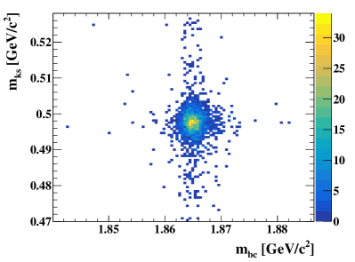
Figure 1: Distribution of $m_{ks}$ versus $m_{bc}$ of the untagged sample.

The analysis requires accurate determination of the signal yields of tagged and untagged samples. The background that passes our selection can be categorized according to its distribution in the plane of $m_{ks}$ versus $m_{bc}$:

• Non-$K^{0}_{\scriptscriptstyle S}$ background: The final state of the signal decay is $K^{+}\kern-1.60004ptK^{-}(\pi^{+}\pi^{-})_{K^{0}_{\scriptscriptstyle S}}$. Events that do not contain the intermediate decay of a $K^{0}_{\scriptscriptstyle S}$ show up as a peak in $m_{bc}$ and a flat distribution in $m_{ks}$.

• Combinatorial background: Events which do not contain the correct final state. These events come from $q\overline{q}$ production and from misreconstructed $D$ decays. The $m_{bc}$ distribution has a phase space component and a wide peak component. The $\pi^{+}\pi^{-}$ pair can, but does not have to originate from a $K^{0}_{\scriptscriptstyle S}$ decay. In case of an intermediate $K^{0}_{\scriptscriptstyle S}$ decay the events show up as a band along $m_{ks}$. Otherwise they are broadly distributed.

The distribution of $m_{ks}$ versus $m_{bc}$ of the untagged sample is shown in Fig. 1. Since the signal peaks in the center of the $m_{bc}$ versus $m_{ks}$ plane, the signal and both background components can be distinguished in data by a fit procedure.

We use an unbinned extended two-dimensional maximum likelihood fit to determine the signal yields. Since the variables $m_{ks}$ and $m_{bc}$ are almost independent the two-dimensional probability density function (PDF) is constructed as a product of the one-dimensional PDFs. The signal components $S^{bc}(m_{bc})$ and $S^{ks}(m_{ks})$ are both modeled by a Crystal Ball function Gaiser (1982) with two-sided power law tails

$$S(x)=\begin{cases}(\frac{n_{L}}{|\alpha_{L}|})^{n_{L}}e^{-\frac{|\alpha_{L}|^{2}}{2}}(\frac{n_{L}}{|\alpha_{L}|}-|\alpha_{L}|-x)^{-n_{L}}\\ e^{-\frac{x^{2}}{2}}\\ (\frac{n_{R}}{|\alpha_{R}|})^{n_{R}}e^{-\frac{|\alpha_{R}|^{2}}{2}}(\frac{n_{R}}{|\alpha_{R}|}-|\alpha_{R}|+x)^{-n_{R}},\end{cases}$$ (3)

with $x=(m-\mu)/\sigma$. The three function components are defined for the lower tail $x<\alpha_{L}$, the central part $\alpha_{L}<x<\alpha_{R}$ and the higher tail $x>\alpha_{R}$. $S^{bc}$ and $S^{ks}$ have separate shape parameters $\mu,\sigma,n_{R},n_{L},\alpha_{R}$ and $\alpha_{L}$.

The combinatorial background model for $m_{bc}$ consists of an ARGUS phase space shape $A(m_{bc})$ Albrecht et al. (1989) and a Gaussian $G_{c}(m_{bc})$. The $m_{ks}$ shape is described by a polynomial of first order $P^{(1)}$ and a peaking component modeled by the $m_{ks}$ shape of the signal

$$B_{c}^{bc}(m_{bc}) =f^{bc}_{c}A(m_{bc})+(1-f^{bc}_{c})G_{c}(m_{bc})$$ (4)

$$B_{c}^{ks}(m_{ks}) =f^{ks}_{c}P^{(1)}_{c}(m_{ks})+(1-f^{ks}_{c})S^{ks}(m_{ks}).$$

The non-$K^{0}_{\scriptscriptstyle S}$ background model has the same shape as the signal in $m_{bc}$ and a polynomial of first order $P^{(1)}$ in $m_{ks}$

$$B_{k}^{bc}(m_{bc}) =S^{bc}(m_{bc})$$ (5)

$$B_{k}^{ks}(m_{ks}) =P^{(1)}_{k}(m_{ks}).$$

The untagged sample additionally contains non-$K^{0}_{\scriptscriptstyle S}$ background candidates which were reconstructed from tracks of the ’tag’ decay. We model these candidates by additional terms $A(m_{bc})$ and $S^{ks}(m_{ks})$ in $B_{k}^{bc}(m_{bc})$ and $B_{k}^{ks}(m_{ks})$, respectively.

Shape parameters are determined using a simultaneous fit to MC samples representing signal and background components. The shape parameters, except the parameter $\sigma$ of the $K^{0}_{\scriptscriptstyle S}$ signal peak, are fixed afterwards. The complete PDF is given by

$$F(m_{bc},m_{ks})= N_{s}\ S^{bc}(m_{bc})S^{ks}(m_{ks})$$

$$+N_{c}\ B_{c}^{bc}(m_{bc})B_{c}^{ks}(m_{ks})$$ (6)

$$+N_{k}\ B_{k}^{bc}(m_{bc})B_{k}^{ks}(m_{ks}).$$

The yields $N_{s}$, $N_{c}$ and $N_{k}$ are determined by an extended maximum likelihood fit to the data sample. This procedure is used for the determination of the untagged signal yield for the branching fraction measurement. The tagged signal fraction for the Dalitz plot analysis is determined by a maximum likelihood fit with fixed sample yield. The fit to the untagged sample is shown in Fig. 2 and yields $11\,660\pm 118.$ signal candidates. For the tagged sample we require additionally to the description in Section III.1 that all candidates are within a box in the $m_{ks}$ versus $m_{bc}$ plane. We choose a box of $\pm$4$$ times the peak width $\sigma$ around the peak maximum in $m_{bc}$ and $m_{ks}$, respectively. The signal yield determined by the fit within this box is $1856\pm 45.$ tagged signal candidates with a purity of $96.37\text{\,}\mathrm{\char 37\relax}$.

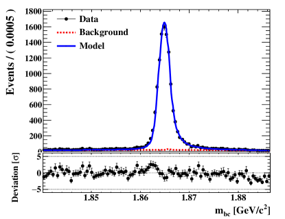
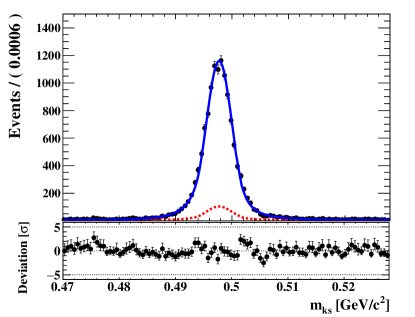
Figure 2: Projections of the untagged data sample and the fit model. Below the deviation between fit model and data sample is shown in units of its uncertainty.

IV Dalitz plot analysis

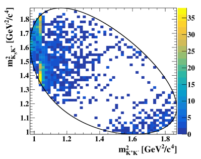
Figure 3: Dalitz plot of the decay $D^{0}\rightarrow K^{0}_{\scriptscriptstyle S}K^{+}\kern-1.60004ptK^{-}$ from the tagged sample. The phase space boundary is indicated.

The Dalitz plot of the decay $D^{0}\rightarrow K^{0}_{\scriptscriptstyle S}K^{+}\kern-1.60004ptK^{-}$ after reconstruction and selection is shown in Fig. 3. Track momenta are updated according to the kinematic fit, described in Section III.1. The distribution is dominated by the $\phi(1020)$ and the $K\kern 1.99997pt\overline{\kern-1.99997ptK}{}$ $S$-wave which in turn is usually described by the charged and neutral $a_{0}(980)$ resonances. The $a_{0}(980)$ mass is below the $K\kern 1.99997pt\overline{\kern-1.99997ptK}{}$ threshold and therefore only its high-mass tail is visible. From the distribution along the $K^{0}_{\scriptscriptstyle S}K^{+}$ invariant mass the vector nature of the $\phi(1020)$ can be observed.

In the following, the free parameters of the Dalitz amplitude model are denoted with $\boldsymbol{\beta}$ and the Dalitz variables with $\boldsymbol{\xi}$. The latter can be either two invariant masses (as used in Fig. 3) or an invariant mass and the corresponding helicity angle (see Eq. 24). The Dalitz plot analysis is performed using the ComPWA framework Michel et al. (2014); Fritsch et al. (2019).

IV.1 Background

The Dalitz plot of background candidates is studied using an MC background sample as well as data and MC sideband samples. Sideband sample events are required to lie outside a box region of $\pm 5$ times the peak width in $m_{bc}$ and $m_{ks}$, and within $1.840<m_{bc}<1.8865$ GeV/c² and $0.470<m_{ks}<0.528$ GeV/c². The comparison of the MC samples with the data sample shows a good agreement (Fig. 4), and the MC background sample is used in the following to fix the shape of a phenomenological background model. A peaking component originates from the decay $D^{0}\rightarrow(KK)_{\phi}(\pi\pi)_{\rho}$. The $\phi(1020)$ is generated unpolarized; the effects of any spin alignment are expected to be negligible. We describe it by a Breit-Wigner model with mass and width parameters of the $\phi(1020)$ and spin zero. An additional Breit-Wigner component with free parameters improves the fit quality close to the $\phi(1020)$ peak. Combinatorial background is described by a phase space component. The background model shows good agreement with sideband data, as shown in Fig. 4. We find $\chi^{2}/\text{ndf}=116/99$ for the comparison of the model and sideband data.

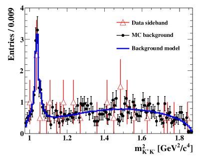
Figure 4: Projection of the MC background sample (full dotted points) and the background model (line) on $m_{KK}^{2}$, both scaled to the expected number of background candidates. The data sideband sample (open triangles) is scaled to approximate the MC background and is also re-binned due to low statistics. Note that zero entries are not plotted.

IV.2 Quantum entangled $D^{0}{\kern-1.60004pt\kern 1.99997pt\overline{\kern-1.99997ptD}\rule{0.0pt}{6.45831pt}{}^{0}}$ decays

We analyze $D^{0}$ mesons produced in the reaction $e^{+}e^{-}\rightarrow D^{0}{\kern-1.60004pt\kern 1.99997pt\overline{\kern-1.99997ptD}\rule{0.0pt}{6.45831pt}{}^{0}}$ via a $\psi(3770)$ as intermediate state. In contrast to an isolated $D^{0}$ decay, this has implications for the decay rate since fundamental conservation laws hold for the combined $D^{0}{\kern-1.60004pt\kern 1.99997pt\overline{\kern-1.99997ptD}\rule{0.0pt}{6.45831pt}{}^{0}}$ decay amplitude and not just for the decay amplitude of one $D^{0}$. We mention especially the conservation of charge-parity ($C\!P$) which we assume to be strictly conserved in the $D^{0}$ system. We follow the phase convention

$$C\!P\ket{D^{0}}=-\ket{\kern 1.99997pt\overline{\kern-1.99997ptD}\rule{0.0pt}{6.45831pt}{}^{0}}.$$ (7)

The decay is mediated by the decay operator $\mathcal{H}$. In the following, the transition amplitude $\matrixelement{j}{\mathcal{H}}{D^{0}}$ of an isolated $D^{0}$ decay to the final state $j$ is denoted by ${\mathcal{A}}_{j}$. From $C\!P$ conservation it follows

$${\mathcal{A}}_{j}=\matrixelement{j}{\mathcal{H}}{D^{0}} =-\matrixelement{{\overline{\jmath}}}{\mathcal{H}}{\kern 1.99997pt\overline{\kern-1.99997ptD}\rule{0.0pt}{6.45831pt}{}^{0}}=-\kern 1.99997pt\overline{\kern-1.99997pt{\mathcal{A}}}{}_{{\overline{\jmath}}}$$

$$\kern 1.99997pt\overline{\kern-1.99997pt{\mathcal{A}}}{}_{j}=\matrixelement{j}{\mathcal{H}}{\kern 1.99997pt\overline{\kern-1.99997ptD}\rule{0.0pt}{6.45831pt}{}^{0}} =-\matrixelement{{\overline{\jmath}}}{\mathcal{H}}{D^{0}}=-{\mathcal{A}}_{{\overline{\jmath}}}.$$ (8)

In the case that $j$ is a $C\!P$ eigenstate we have $j={\overline{\jmath}}$ and we include the $C\!P$ eigenvalue $\eta$ of the final state $j$: ${\mathcal{A}}_{j}=-\eta\kern 1.99997pt\overline{\kern-1.99997pt{\mathcal{A}}}{}_{j}$. We describe the amplitude ratio of $D^{0}$ and $\kern 1.99997pt\overline{\kern-1.99997ptD}\rule{0.0pt}{6.45831pt}{}^{0}$ to the same final state $j$ using its magnitude $r_{j}$ and phase $\delta_{j}$

$$\lambda_{j}=\frac{{\mathcal{A}}_{j}}{\kern 1.99997pt\overline{\kern-1.99997pt\mathcal{A}}{}_{j}}=-r_{j}e^{-i\delta_{j}}.$$ (9)

In general, the amplitudes ${\mathcal{A}}_{j}$ depend on the phase space position: ${\mathcal{A}}_{j}$ is constant only for two-body decays. We denote those final states with $r_{j}\leq 1$ by $j$ and their charge-conjugates with $r_{{\overline{\jmath}}}>1$ by ${\overline{\jmath}}$.

The combined wave function of $D^{0}{\kern-1.60004pt\kern 1.99997pt\overline{\kern-1.99997ptD}\rule{0.0pt}{6.45831pt}{}^{0}}$ is anti-symmetric due to the negative parity of the $e^{+}e^{-}$ reaction. The matrix element of the decay of $D^{0}$ and $\kern 1.99997pt\overline{\kern-1.99997ptD}\rule{0.0pt}{6.45831pt}{}^{0}$ to the final states $i$ and $j$ at decay times $t_{1}$ and $t_{2}$, respectively, is given by

$${\mathcal{M}}_{ij}(t_{1},t_{2})= \frac{1}{\sqrt{2}}\bigg{[}\matrixelement{i}{\mathcal{H}}{D^{0}(t_{1})}\matrixelement{j}{\mathcal{H}}{\kern 1.99997pt\overline{\kern-1.99997ptD}\rule{0.0pt}{6.45831pt}{}^{0}(t_{2})}$$

$$-\matrixelement{i}{\mathcal{H}}{\kern 1.99997pt\overline{\kern-1.99997ptD}\rule{0.0pt}{6.45831pt}{}^{0}(t_{1})}\matrixelement{j}{\mathcal{H}}{D^{0}(t_{2})}\bigg{]}.$$ (10)

The BESIII experiment does not give access to the $D^{0}$ decay time and therefore we are only interested in the time-integrated transition matrix element. The integration of Eq. 10 over the $D^{0}$ decay time difference yields

$$\absolutevalue{{\mathcal{M}}_{ij}}^{2} =\int_{-\infty}^{\infty}\absolutevalue{{\mathcal{M}}_{ij}(\absolutevalue{t_{2}-t_{1}})}^{2}\ d(\absolutevalue{t_{2}-t_{1}})$$

$$\approx\absolutevalue{\kern 1.99997pt\overline{\kern-1.99997pt\mathcal{A}}{}_{j}{\mathcal{A}}_{i}-{\mathcal{A}}_{j}\kern 1.99997pt\overline{\kern-1.99997pt\mathcal{A}}{}_{i}}^{2}.$$ (11)

We choose the normalization such that $\absolutevalue{{\mathcal{M}}_{ij}}^{2}$ and $\absolutevalue{{\mathcal{A}}_{i}}^{2}$ are branching fractions when integrated over the phase space. The $D^{0}$ mixing parameters $x$ and $y$ are of $\mathcal{O}$ ($10^{-3}$) (Tanabashi et al., 2018, p. 691ff) and thus are neglected in second order in the previous expression.

Using Eq. 9 we can write Eq. 11 as

$$\absolutevalue{{\mathcal{M}}_{ij}}^{2} \approx\absolutevalue{\kern 1.99997pt\overline{\kern-1.99997pt\mathcal{A}}{}_{j}{\mathcal{A}}_{i}-{\mathcal{A}}_{j}\kern 1.99997pt\overline{\kern-1.99997pt\mathcal{A}}{}_{i}}^{2}$$

$$=\absolutevalue{\kern 1.99997pt\overline{\kern-1.99997pt\mathcal{A}}{}_{i}}^{2}\absolutevalue{\kern 1.99997pt\overline{\kern-1.99997pt\mathcal{A}}{}_{j}\lambda_{i}-{\mathcal{A}}_{j}}^{2}.$$ (12)

For our case we get

$$\absolutevalue{{\mathcal{M}}_{\text{tag},3K}}^{2} =\absolutevalue{\kern 1.99997pt\overline{\kern-1.99997pt\mathcal{A}}{}_{\text{tag}}}^{2}\absolutevalue{\kern 1.99997pt\overline{\kern-1.99997pt\mathcal{A}}{}_{3K}\lambda_{\text{tag}}-{\mathcal{A}}_{3K}}^{2}.$$ (13)

The decay amplitudes of $D^{0}$ $\rightarrow$ $K^{0}_{\scriptscriptstyle S}K^{+}\kern-1.60004ptK^{-}$ and $\kern 1.99997pt\overline{\kern-1.99997ptD}\rule{0.0pt}{6.45831pt}{}^{0}$ $\rightarrow$ $K^{0}_{\scriptscriptstyle S}K^{+}\kern-1.60004ptK^{-}$ are connected via Libby et al. (2010)

$$\kern 1.99997pt\overline{\kern-1.99997pt\mathcal{A}}{}_{3K}(m_{K^{0}K^{+}}^{2}, m_{K^{0}K^{-}}^{2})$$

$$={\mathcal{A}}_{3K}(m_{K^{0}K^{-}}^{2},m_{K^{0}K^{+}}^{2})$$ (14)

if $C\!P$ is conserved. The amplitude of the flavor tag decay ${\mathcal{A}}_{\text{tag}}$ does not depend on the phase space position of the signal decay and is therefore constant in Eq. 13. The ratio of $D^{0}$ to $\kern 1.99997pt\overline{\kern-1.99997ptD}\rule{0.0pt}{6.45831pt}{}^{0}$ amplitude of the tag decay is denoted by

$$\lambda_{\text{tag}}=-r_{D}e^{-i\delta_{D}}.$$ (15)

We use experimental input for the magnitude and phase of $\lambda_{\text{tag}}$. Since these parameters have not yet been measured for each tag channel separately, we set them to common values for all tag channels. As nominal value we choose the experimental average for the final state $K^{-}\pi^{+}$. Experimental results are summarized in Table 2.

Table 2: Hadronic parameters of tag channels. The mixing parameters and the hadronic parameters for the final state $K\pi$ are obtained by a global fit Amhis et al. (2019). The measurement for $K\pi\pi^{0}$ and $K^{-}\pi^{+}\pi^{-}\pi^{+}$ are from Evans et al. (2016). For the other tag channels no measurements exist today.

Parameter	Value
$x$	$0.50\pm 0.14\text{\,}\mathrm{\char 37\relax}$
$y$	$0.62\pm 0.07\text{\,}\mathrm{\char 37\relax}$
$\left(r_{D}^{K\pi}\right)^{2}$	$0.344\pm 0.002\text{\,}\mathrm{\char 37\relax}$
$\delta_{K\pi}$	$9.8\pm 8.6\text{\,}\mathrm{\SIUnitSymbolDegree}$
$r_{D}^{K\pi\pi^{0}}$	$4.48\pm 0.12\text{\,}\mathrm{\char 37\relax}$
$\delta_{K\pi\pi^{0}}$	$19\pm 14.\text{\,}\mathrm{\SIUnitSymbolDegree}$
$r_{D}^{{\mathrm{K}3\pi}}$	$5.50\pm 0.12\text{\,}\mathrm{\char 37\relax}$
$\delta_{K3\pi}$	$-55\pm 18.\text{\,}\mathrm{\SIUnitSymbolDegree}$

A detailed derivation of the decay amplitude of quantum entangled $D^{0}$ mesons is given in Tanabashi et al. (2018); Asner and Sun (2006). To summarize, the result of an analysis of the $D^{0}\rightarrow K^{0}_{\scriptscriptstyle S}K^{+}\kern-1.60004ptK^{-}$ Dalitz plot needs to be the amplitude model of an isolated $D^{0}$ decay in order to be comparable with other $D^{0}$ production reactions (e. g. $D^{*}\rightarrow D^{0}\pi$). Therefore, the effect of the production mechanism needs to be considered in the amplitude model. For many $D^{0}$ final states this effect can be neglected, but it needs to be considered in this analysis since $K^{0}_{\scriptscriptstyle S}K^{+}\kern-1.60004ptK^{-}$ is a self-conjugate final state. The effect of the quantum entanglement on the measurement of the branching fraction is discussed in Section V.1.

IV.3 Resonance model

The signal decay amplitude ${\mathcal{A}}_{3K}$ is parameterized in the isobar model using the helicity formalism. The dynamic parts are described by a Breit-Wigner formula and, in the case of the $K\kern 1.99997pt\overline{\kern-1.99997ptK}{}$ $S$-wave, by a Flatté description. We consider an intermediate resonance $R$ produced in the initial state $i$ and decaying to the final state $f$ with final state particles $a$ and $b$. The third (spectator) particle in the three-body decay is denoted by $c$. The resonance has the angular momentum $J$ and its parameterization depends on the center-of-mass energy squared $s$ of the final state particles $a$ and $b$.

The Breit-Wigner description suggested by the PDG Tanabashi et al. (2018) is

$$R^{J}(s)=-\frac{g_{D\rightarrow R}\ g_{R\rightarrow f}}{m_{R}^{2}-s+i\sqrt{s}\Gamma(s)},$$ (16)

with the mass dependent width

$$\Gamma(s)=\Gamma_{R}\left(\frac{q(s)}{q(m_{R}^{2})}\right)^{2J+1}\left(\frac{m_{R}}{\sqrt{s}}\right)\frac{F_{J}^{2}(z)}{F_{J}^{2}(z_{R})}.$$ (17)

The center-of-mass daughter momentum $q(s)$ is imaginary below threshold. Therefore, we derive it from an analytic continuation of the phase-space factor:

$$i\rho=\begin{cases}-\frac{\hat{\rho}}{\pi}\log{\absolutevalue{\frac{1+\hat{\rho}}{1-\hat{\rho}}}},&s<0\\ -\frac{2\hat{\rho}}{\pi}\arctan{\frac{1}{\hat{\rho}}},&0<s<s_{{\textrm{th}}}\\ -\frac{\hat{\rho}}{\pi}\log{\absolutevalue{\frac{1+\hat{\rho}}{1-\hat{\rho}}}}+i\hat{\rho},&s_{{\textrm{th}}}<s\\ \end{cases}.$$ (18)

with

$$\hat{\rho}(s)=\frac{1}{16\pi}\frac{2\sqrt{\absolutevalue{\hat{q}(s)}^{2}}}{\sqrt{s}},$$ (19)

and

$$\hat{q}^{2}(s)=\frac{(s-(m_{a}+m_{b})^{2})(s-(m_{a}-m_{b})^{2})}{4s}.$$ (20)

Eq. 19 is input to Eq. 18 and is in turn used to calculate $q(s)$ from the resulting $\rho$. This is the parameterization suggested by the PDG (Tanabashi et al., 2018, Section 48.2.3).

The coupling constants for the production and decay $g_{i}$ in Eq. 16 are related to the partial width $\Gamma_{i}$ via

$$g_{R\rightarrow f}=\frac{1}{q^{J}(s_{R})F_{J}(z_{R})}\sqrt{\frac{m_{R}\Gamma_{R\rightarrow f}}{\rho(s)}}.$$ (21)

This relation holds for narrow and isolated resonances.

The Breit-Wigner model assumes a point-like object. The effect of an extended resonance object is taken into account via the angular momentum barrier factors $F_{J}^{2}(z)$. The Blatt-Weisskopf barrier factors Blatt and Weisskopf (1979) are widely used:

$$F_{0}^{2}(z) =1$$

$$F_{1}^{2}(z) =\frac{2z}{z+1}$$ (22)

$$F_{2}^{2}(z) =\frac{13z^{2}}{(z-3)^{2}+9z},$$

where $z(s)=q(s)^{2}R^{2}$. Experience shows that the influence of the resonance radius $R$ is rather small. We use $R=$1.5\text{\,}\mathrm{G}\mathrm{eV}^{-1}$$.

The $K\kern 1.99997pt\overline{\kern-1.99997ptK}{}$ $S$-wave involves the charged and neutral $a_{0}(980)$. The $a_{0}(980)$ couples strongly to the channel $K\kern 1.99997pt\overline{\kern-1.99997ptK}{}$ as well as to the channel $\eta\pi$. We describe both by a coupled channel formula, the so-called Flatté formula Flatte (1976). We use the parameterization from Ref. Aubert et al. (2005):

$$R^{J}_{2ch}(s)=-\frac{g_{D\rightarrow R}\ g_{K\kern 1.39998pt\overline{\kern-1.39998ptK}{}}}{m_{R}^{2}-s+i(g_{K\kern 1.39998pt\overline{\kern-1.39998ptK}{}}^{2}\rho_{K\kern 1.39998pt\overline{\kern-1.39998ptK}{}}+g_{\eta\pi}^{2}\rho_{\eta\pi})}.$$ (23)

The coupling constants are denoted by $g_{i}$ and the phase space factor $\rho_{i}$ is given in Eq. 18. The $a_{0}(980)^{0}$ couples also to the channel $K^{0}\kern-1.60004pt\kern 1.99997pt\overline{\kern-1.99997ptK}{}^{0}$. Consequently, we add a third channel to the denominator of Eq. 23 with the same coupling as the $K^{+}\kern-1.60004ptK^{-}$ channel. Other than this difference, the $a_{0}(980)^{0}$ and $a_{0}(980)^{+}$ use the same values for their coupling constants.

The decay $D^{0}\rightarrow K^{0}_{\scriptscriptstyle S}K^{+}\kern-1.60004ptK^{-}$ is a decay of a pseudo-scalar particle to three final state pseudo-scalar particles. The angular distribution of an intermediate resonance is therefore given by the Legendre polynomials $P_{J}(\cos\theta_{R})$, which depend on the helicity angle

$$\cos\theta_{R}=-\frac{m^{2}_{ac}-m^{2}_{a}-m^{2}_{c}-2E_{R}^{*}E_{c}^{*}}{2q_{R}^{*}q_{c}^{*}}.$$ (24)

Starred quantities are measured in the rest frame of the resonance.

The total decay amplitude ${\mathcal{A}}_{j}$ to a final state $j$ is the coherent sum over the individual resonances

$${\mathcal{A}}_{j}(\boldsymbol{\xi},\boldsymbol{\beta})=\sum_{J} \frac{\sqrt{2J\!+\!1}}{4\pi}\times$$

$$\sum_{i}c_{i}n_{i}R_{i}^{J}(s_{i}^{2})P_{J}(\cos\theta_{i}).$$ (25)

The prefactor originates from the normalization of the Legendre polynomials. The Dalitz plot variables are denoted by $\boldsymbol{\xi}$ and consist of invariant mass $s_{i}^{2}$ and helicity angle $\theta_{i}$ for each subsystem.

The magnitude and phase are given by the complex coefficient $c_{i}$, and all resonances are normalized with the factors

$$n_{i}^{-1}=\int\differential{\boldsymbol{\xi}}R_{i}^{J}(\boldsymbol{\xi},\boldsymbol{\beta}).$$ (26)

We insert ${\mathcal{A}}(\boldsymbol{\xi},\boldsymbol{\beta})$ into Eq. 13 to obtain the decay amplitude including the effect of the quantum entanglement of $D^{0}$ and $\kern 1.99997pt\overline{\kern-1.99997ptD}\rule{0.0pt}{6.45831pt}{}^{0}$.

IV.4 Likelihood function

The probability function is given by

$$L(\boldsymbol{\xi},\boldsymbol{\beta})= f\cdot\frac{\absolutevalue{{\mathcal{M}}(\boldsymbol{\xi},\boldsymbol{\beta})}^{2}}{\int|{\mathcal{M}}(\boldsymbol{\xi}^{\prime},\boldsymbol{\beta})|^{2}\epsilon(\boldsymbol{\xi}^{\prime})\differential{\boldsymbol{\xi}^{\prime}}}$$

$$+(1-f)\cdot\absolutevalue{B(\boldsymbol{\xi})}^{2}.$$ (27)

$B(\boldsymbol{\xi})$ denotes the Dalitz plot background model. The efficiency function is denoted by $\epsilon(\boldsymbol{\xi})$ and the signal purity by $f=($96.37$\pm$0.43$({\textrm{stat.}}))~{}$\mathrm{\char 37\relax}$$. The normalization integrals are calculated with MC integration using a sample of phase space distributed candidates which have passed reconstruction and selection. In this way the efficiency correction is incorporated without the need to explicitly parameterize $\epsilon(\boldsymbol{\xi})$. The likelihood function is evaluated for each event, and the logarithm of its products can be written as

$$-\log{{\mathcal{L}}}(\boldsymbol{\beta})=-\sum_{\text{ev}}^{N}\log L(\boldsymbol{\xi}_{\text{ev}},\boldsymbol{\beta}),$$ (28)

where $N$ is the size of the data sample. The interesting physics parameters are the fit fractions which are defined as

$$f_{i}=\frac{|c_{i}|^{2}\int\differential{\boldsymbol{\xi}}n_{i}^{2}\absolutevalue{R_{i}(\boldsymbol{\xi},\boldsymbol{\beta})}^{2}}{\int\differential{\boldsymbol{\xi}}\absolutevalue{{\mathcal{M}}(\boldsymbol{\xi},\boldsymbol{\beta})}^{2}},$$ (29)

where $c_{i}$ is the magnitude of resonance $R_{i}$. The integral $\int\differential{\boldsymbol{\xi}}n_{i}^{2}\absolutevalue{R_{i}(\boldsymbol{\xi})}^{2}$ is equal to one, due to our choice for the resonance normalization (Eq. 26). A precise calculation of the statistical uncertainty of the fit fractions requires the propagation of the full covariance matrix through the integration which is achieved using an MC approach.

IV.5 Model selection

Table 3: Overview of resonances that could appear as intermediate states. Mass and width are the Breit-Wigner parameters. In case that these are channel dependent we quote the parameters of the $K\kern 1.99997pt\overline{\kern-1.99997ptK}{}$ final state. The parameters of $f_{0}(980)$ and $a_{0}(980)$ are weighted averages of previous measurements of Refs. Ambrosino et al. (2007); Garcia-Martin et al. (2011); Ablikim et al. (2005) and Refs. Teige et al. (1999); Abele et al. (1998); Bugg (2008); Ambrosino et al. (2009); Athar et al. (2007); Adams et al. (2011), respectively. The other values are from the PDG Patrignani et al. (2016).

Resonance $I^{G}$ ($J^{PC}$) Mass [$\mathrm{M/}$] Coupling $f_{0}(980)$ $0^{+}(0^{++})$ $971\pm 7.$ $g_{K\kern 1.39998pt\overline{\kern-1.39998ptK}{}}=$ $3.54\pm 0.05\text{\,}\mathrm{GeV}$ $g_{\pi\pi}=$ $1.5\pm 0.1\text{\,}\mathrm{GeV}$ $a_{0}(980)$ $1^{-}(0^{++})$ $$994$^{$6$}_{$-4$}$ $g_{\eta\pi}=$ $2.66\pm 0.04\text{\,}\mathrm{GeV}$ $\phi(1020)$ $0^{-}(1^{--})$ $1019.461\pm 0.019$ $\Gamma=$ $4.266\pm 0.031\text{\,}\mathrm{MeV}$ $f_{2}(1270)$ $0^{+}(2^{++})$ $1275.5\pm 0.8$ $\Gamma=$ $($185.9$^{$2.8$}_{$-2.1$})$\mathrm{MeV}$$ $a_{2}(1320)$ $1^{-}(2^{++})$ $1318.1\pm 0.7$ $\Gamma_{K\kern 1.39998pt\overline{\kern-1.39998ptK}{}}=$ $109.8\pm 2.4\text{\,}\mathrm{MeV}$ $f_{0}(1370)$ Vladimirsky et al. (2006) $0^{+}(0^{++})$ $1440\pm 6.$ $\Gamma_{K\kern 1.39998pt\overline{\kern-1.39998ptK}{}}=$ $121\pm 15.\text{\,}\mathrm{MeV}$ $a_{0}(1450)$ $1^{-}(0^{++})$ $1474\pm 19.$ $\Gamma=$ $256\pm 13.\text{\,}\mathrm{MeV}$

The PDG Tanabashi et al. (2018) lists 12 resonances that could potentially contribute to the decay $D^{0}\rightarrow K^{0}_{\scriptscriptstyle S}K^{+}\kern-1.60004ptK^{-}$. Due to the limited size of the data sample we consider only resonance that were found to decay to $K\kern 1.99997pt\overline{\kern-1.99997ptK}{}$ by previous experiments. An overview of known resonances is given in Table 3. The choice of resonances that are included in the model is a common problem in amplitude analysis. Generally, increasing the complexity of the model improves the fit quality. In the usual approach, a minimum statistical significance or a minimum fit fraction (or both) is required for each resonance. Those requirements are somewhat arbitrary parameters and furthermore, the order in which resonances are added (or removed) from the model can lead to different sets of resonances. We apply a more abstract method for resonance selection.

Balancing a model between fit quality and model complexity is a common problem in the area of machine learning and in statistics in general. One approach to solve such a problem is the so-called Least Absolute Shrinkage and Selection Operator (LASSO) method Tibshirani (1996). The basic idea is to penalize undesired behavior of the objective function. In the original approach the objective function is a least square model and the penalty function is the sum of the absolute values of the free parameters. In the context of particle physics this approach is described in Guegan et al. (2015). In our case the objective function is the logarithm of the likelihood, and the undesired behavior is a large sum over all fit fractions (which indicates strong interferences). Therefore, we use the sum of the square-root of fit fractions as penalty function. We modify Eq. 28

$$-\log{{\mathcal{L}}_{\lambda_{P}}} (\boldsymbol{\beta})=-\log{{\mathcal{L}}}(\boldsymbol{\beta})$$ (30)

$$+\lambda_{P}\sum_{i}\sqrt{\frac{\int\differential\boldsymbol{\xi}\ N_{i}^{2}R_{i}R_{i}^{*}}{\int\differential\boldsymbol{\xi}\ \sum\limits_{m,n}N_{m}N_{n}R_{m}R_{n}^{*}}}.$$

The square-root is used since it favors the suppression of small contributions, in contrast to, for example, the sum of the fit fractions which would favor solutions with equal values.

The parameter $\lambda_{P}$ regularizes the model complexity. A large value suppresses the sum of fit fractions and small values allow for larger interference terms. It is a nuisance parameter and we have to determine its optimal value. Again, this is a common problem in statistics and a possible solution is the use of so-called information criteria. Information criteria are mathematical formulations of the ‘principle of parsimony’ Schwarz (1978). This means in hypothesis testing that we prefer the model with fewer parameters over a more complicated model, given the same goodness-of-fit. The criteria suggested by Guegan et al. (2015) are the Akaike information criteria (AIC) Akaike (1974) and Bayesian information criteria (BIC) Schwarz (1978). We choose a slightly modified version of the AIC which takes the size of the data sample into account:

$${\textrm{AIC}}^{\lambda_{P}}_{c}=-2\log{{\mathcal{L}}}_{\lambda_{P}}+2r_{\lambda_{P}}+\frac{2r(r+1)}{N-r-1}.$$ (31)

The number of events in data is denoted by $N$ and the coefficient $r$ is related to the complexity of the model. We follow the suggestion in Ref. Guegan et al. (2015) and use the number of resonances as parameter $r$. We consider only resonances with a fit fraction larger than a minimum value. A minimum value of $2\text{\times}{10}^{-3}$ gives a stable result.

A scan for different values of $\lambda_{P}$ over a wide range is performed to map out the minima of $AIC^{\lambda_{P}}_{c}$. The scan is shown in Fig. 5 and a minimum at $\lambda_{P}^{min}=$9.0$$ is found. The final set of resonances is stable versus small variations of $\lambda_{P}$. After a set of resonances is selected the penalty term is removed from the likelihood.

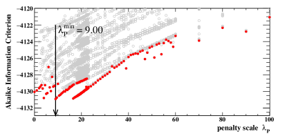
Figure 5: Distribution of $AIC^{\lambda_{P}}_{c}$ versus the penalty scale $\lambda_{P}$. A minimum is found at $\lambda_{P}^{min}=$9.0$$. For each value of $\lambda_{P}$ several fits with different starting parameters are performed (gray circles). Only the result with the lowest value (red dots) is considered.

We obtain a model consisting of $a_{0}(980)^{0}$, $a_{0}(980)^{+}$, $\phi(1020)$, $a_{2}(1320)^{+}$, $a_{2}(1320)^{-}$ and $a_{0}(1450)^{-}$. The model contains the $a_{2}(1320)^{-}$ and $a_{0}(1450)^{-}$ which are expected to be doubly Cabibbo-suppressed with regard to their positively charged partner. We suspect that those contributions appear as an artefact of an imperfect model description in some phase space regions. We therefore decide to quote additionally a ‘basic’ model of $a_{0}(980)^{0}$, $a_{0}(980)^{+}$ and $\phi(1020)$.

IV.6 Goodness-of-fit

The distribution of data events across the Dalitz plot is not uniform, and in a larger area of the phase space almost no events are observed (see Fig. 3). Therefore, we apply a goodness-of-fit test which is more suitable for this situation than the widely used $\chi^{2}$ test. We choose a point-to-point dissimilarity method Aslan and Zech (2005) which provides an unbinned goodness-of-fit test. The test variable $\Phi$ is defined as

$$\Phi=\frac{1}{2}\int \differential\boldsymbol{\xi}\int\differential\boldsymbol{\xi}^{\prime}\left[\rho_{m}(\boldsymbol{\xi})-\rho_{n}(\boldsymbol{\xi})\right]$$

$$\left[\rho_{m}(\boldsymbol{\xi}^{\prime})-\rho_{n}(\boldsymbol{\xi}^{\prime})\right]R(\absolutevalue{\boldsymbol{\xi}-\boldsymbol{\xi}^{\prime}}).$$ (32)

We use the Euclidean metric to calculate the distance between two points in phase space. For the general distance function $R(\absolutevalue{\boldsymbol{\xi}-\boldsymbol{\xi}^{\prime}})$ we choose a Gaussian function with a width which is proportional to the amplitude value. The underlying (in general unknown) PDFs of two samples are denoted $\rho_{m}$ and $\rho_{n}$. Therefore, we estimate $\rho_{m}$ and $\rho_{n}$ by MC integration using samples from each PDF

$$\Phi =\frac{1}{N(N+1)}\sum_{j>i}^{N}R(|\mathbf{n_{i}}-\mathbf{n_{j}}|)$$

$$-\frac{1}{NM}\sum_{j,i}^{M,N}R(|\mathbf{n_{i}}-\mathbf{m_{i}}|)$$ (33)

$$+\frac{1}{M(M+1)}\sum_{j>i}^{M}R(|\mathbf{m_{i}}-\mathbf{m_{j}}|).$$

Elements of both samples are denoted by $\mathbf{m_{i}}$ and $\mathbf{n_{i}}$ and the total sample size by $M$ and $N$, respectively. We identify one sample with our data sample, and the second one is generated using the final amplitude model. To calculate a probability that a certain model fits the data, the distribution of the test variable is needed. This can not be analytically derived and we simulate it using an MC approach; the result is given below.

IV.7 Systematics

Systematic uncertainties on the Dalitz plot amplitude model arise from various sources: background description, amplitude model, inaccuracies of the MC simulation, external parameters and the fit procedure. For each source of uncertainty, we rerun the fit with a different configuration and add the deviations from the nominal amplitude model in quadrature. An overview of the systematic uncertainties is given in Table 4.

Table 4: Overview of uncertainties for the Dalitz plot amplitude model. We list the fit parameters and their statistical and systematic uncertainties. The fit parameters and fit fractions are corrected for their fitting biases and are denoted by ‘corrected value’. Systematic uncertainties are given in units of the statistical uncertainty of the parameter $\bar{\sigma}$ (we use the average value of the asymmetric uncertainties).

Parameter $g_{KK}$ $a_{0}(980)^{0}$ $a_{0}(980)^{+}$ $\phi(1020)$ $a_{2}(1320)^{+}$ $a_{2}(1320)^{-}$ $a_{0}(1450)^{-}$ [$\mathrm{GeV}$] FF [$\mathrm{\char 37\relax}$] $\absolutevalue{c}$ $\phi~{}[$\mathrm{rad}$]$ FF [$\mathrm{\char 37\relax}$] $\absolutevalue{c}$ $\phi~{}[$\mathrm{rad}$]$ FF [$\mathrm{\char 37\relax}$] $\absolutevalue{c}$ $\phi~{}[$\mathrm{rad}$]$ FF [$\mathrm{\char 37\relax}$] $\absolutevalue{c}$ $\phi~{}[$\mathrm{rad}$]$ FF [$\mathrm{\char 37\relax}$] $\absolutevalue{c}$ $\phi~{}[$\mathrm{rad}$]$ FF [$\mathrm{\char 37\relax}$] Fit value 3.80 93 0.59 2.96 33 0.71 1.67 47 0.13 $-$2.97 1.5 0.10 $-$0.14 0.9 0.21 $-$0.23 4.1 Corrected value 3.77 90 0.64 2.94 34 0.74 1.67 48 0.12 $-$2.92 1.4 0.09 $-$0.06 0.8 0.16 0.12 2.2 Mean stat. uncertainty $\bar{\sigma}$ 0.24 10 0.11 0.17 7 0.06 0.08 2 0.03 0.23 0.6 0.03 0.23 0.4 0.08 0.58 2.4 Sys. uncertainty 0.35 14 0.09 0.06 6 0.08 0.19 3 0.01 0.31 0.3 0.02 0.28 0.2 0.04 0.50 1.9 Total uncertainty 0.42 17 0.14 0.17 9 0.10 0.21 4 0.03 0.39 0.7 0.03 0.36 0.5 0.10 0.76 3.1 Systematic uncertainties in units of the mean statistical uncertainty $\bar{\sigma}$ Background 0.25 0.71 0.49 0.18 0.53 0.49 0.17 0.29 0.38 0.34 0.27 0.11 0.15 0.17 0.22 0.53 0.21 Amplitude model 0.16 0.27 0.26 0.17 0.33 0.18 0.07 0.09 0.15 0.04 0.10 0.04 0.08 0.12 0.14 0.28 0.14 Quantum correlation 0.04 1.21 0.56 0.24 0.45 1.14 1.65 1.91 0.13 0.32 0.31 0.19 0.21 0.12 0.21 0.52 0.36 External parameters 1.44 0.49 0.15 0.17 0.48 0.36 1.96 0.27 0.09 1.27 0.19 0.56 1.17 0.59 0.31 0.34 0.55 Fitting procedure 0.07 0.17 0.20 0.05 0.13 0.24 0.05 0.23 0.12 0.11 0.08 0.10 0.17 0.09 0.29 0.30 0.41 Sys. uncertainty 1.46 1.50 0.79 0.34 0.86 1.31 2.56 1.97 0.43 1.35 0.46 0.61 1.21 0.64 0.53 0.87 0.80

IV.7.1 Background

Uncertainties from the background treatment come from the background model as well as from the uncertainty on the signal purity. The fit quality of the background model is good as illustrated in Fig. 4, and we do not assign an uncertainty due to our choice of the model but we use different samples to determine the shape parameters. The nominal sample is the MC background sample and we additionally test MC and data sideband samples. The difference of the fit result in comparison to the nominal model is taken as systematic uncertainty. Note that the contribution to the $\phi(1020)$ peak is different for the signal and sideband region. Thus, the systematic uncertainty is a conservative assumption. The effect on the Dalitz plot analysis of the uncertainty on the signal purity is estimated by varying the signal purity by two times its statistical uncertainty to larger and smaller values.

IV.7.2 Amplitude model

A source of uncertainty of the amplitude model is the resonance radius that is used in the barrier factors. We vary it in steps of $1\text{\,}\mathrm{G}\mathrm{eV}^{-1}$ from $0\text{\,}\mathrm{G}\mathrm{eV}^{-1}$ to $5\text{\,}\mathrm{G}\mathrm{eV}^{-1}$. Our nominal value is $1.5\text{\,}\mathrm{G}\mathrm{eV}^{-1}$.

The quantum entanglement of $D^{0}{\kern-1.60004pt\kern 1.99997pt\overline{\kern-1.99997ptD}\rule{0.0pt}{6.45831pt}{}^{0}}$ is included in the Dalitz amplitude model. We use external measurements of the magnitude and phase of $\lambda_{\text{tag}}$ (Eq. 15). The experimental averages for $r_{D}$ and $\delta_{D}$ from the final state $K^{-}\pi^{+}$ are used as nominal values. The influence on the result is studied using the value for $r_{D}$ from $K^{-}\pi^{+}\pi^{0}$ and twice the $K^{-}\pi^{+}$ nominal value. The phase $\delta_{D}$ is set to zero, twice the $K^{-}\pi^{+}$ nominal value and to the measured value of $K^{-}\pi^{+}\pi^{-}\pi^{+}$.

IV.7.3 Monte-Carlo simulation

The efficiency correction of the data sample is obtained from MC simulation. Differences between data and MC simulation in track reconstruction and particle identification can influence the result. Especially, regions with low momentum $K^{\pm}$ tracks are prone to inaccuracies. We correct for these differences using momentum dependent correction factors obtained from hadronic $D^{0}$ decays. We test the influence of the tracking correction by rerunning the fit without correction. The influence is found to be negligible for the Dalitz plot analysis and thus no systematic uncertainty is assigned.

Another effect comes from different momentum resolutions in data and MC simulation. The $\phi(1020)$ has a width that is of the same order as the mass resolution. We study the influence of the mass resolution by rerunning the minimization with a free width parameter which approximates a resolution difference. The parameter changes from $4.266\text{\,}\mathrm{MeV}$ to $5.2\pm 0.3\text{\,}\mathrm{MeV}$. We add the deviation from the nominal model to the systematic uncertainty. We keep the parameter fixed in the nominal fit.

IV.7.4 External parameters

External parameters are listed in Tables 3 and 2. We shift each parameter by its uncertainty to smaller and larger values and rerun the minimization. The deviation from the nominal model is taken as systematic uncertainty. The influence of the $a_{0}(980)$ coupling to $\eta\pi$ is estimated by rerunning the minimization with both couplings as free parameters. We obtain a value of $g_{\eta\pi}=$2.54\pm 0.16\text{\,}\mathrm{GeV}$$.

IV.7.5 Fit procedure

We validate that the analysis routine is bias free and that the fit routine provides a correct estimate of the statistical uncertainty. We use our nominal fit result to generate a signal MC sample. This sample passes detector simulation and reconstruction as well as the event selection procedure. Then, we add the expected amount of background from MC simulation and rerun the minimization procedure. We calculate the difference between the parameters of the nominal model and the fit result in units of the statistical uncertainty of the parameter. The procedure is repeated with $200$ statistically independent samples.

We find that the error estimate is correct but small biases for some parameters are present, especially for the parameters of the $a_{0}(1450)^{-}$. We correct each fit parameter for its bias and add half of the correction to the systematic uncertainty.

Furthermore, we check that no better minimum exists in the parameter space. We do so by rerunning the minimization with start values chosen randomly across the whole parameter space. From $200$ fits, no fit with a valid minimum exhibits a smaller negative logarithm of the likelihood value than the nominal fit.

IV.8 Results

We find that the Dalitz plot is well described by a model with six resonances: $a_{0}(980)^{0}$, $a_{0}(980)^{+}$, $\phi(1020)$, $a_{2}(1320)^{+}$, $a_{2}(1320)^{-}$ and $a_{0}(1450)^{-}$. The Dalitz plot projections and the fit model are shown in Fig. 6 and the fit parameters are listed in Table 5. The magnitude and phase of the $a_{0}(980)^{0}$ are fixed to $1$ and $0$, respectively, as a reference.

Table 5: Result from the Dalitz plot analysis. The first uncertainty is statistical followed by systematic uncertainty. The coupling constant $a_{0}(980)\rightarrow K\kern 1.99997pt\overline{\kern-1.99997ptK}{}$ is determined to be $g_{K\kern 1.39998pt\overline{\kern-1.39998ptK}{}}=($3.77$\pm$0.24$\pm$0.35$)$\mathrm{GeV}$$. For the $a_{2}(1320)^{+}$, $a_{2}(1320)^{-}$ and $a_{2}(1320)^{+}$ the upper limits and the central values (CV) of the fit fractions are quoted as well as their combined significance.

Final state Magnitude Phase [$\mathrm{rad}$] Fit fraction [$\mathrm{\char 37\relax}$] Sign.[$\sigma$] $a_{0}(980)^{0}K^{0}_{\scriptscriptstyle S}$ $1$ $0$ $$90$\pm$10$\pm$17$$ $>$$10$aaaaa $a_{0}(980)^{+}K^{-}$ $$0.64$^{$0.14$}_{$-0.08$}\pm$0.09$$ $$2.94$^{$0.19$}_{$-0.14$}\pm$0.06$$ $$34$\pm$7$\pm$6$$ $>$$10$aaaaa $\phi(1020)K^{0}_{\scriptscriptstyle S}$ $$0.74$^{$0.08$}_{$-0.04$}\pm$0.08$$ $$1.67$\pm$0.08$\pm$0.19$$ $$48$\pm$2$\pm$3$$ $>$$10$aaaaa $a_{2}(1320)^{+}K^{-}$ $$0.12$\pm$0.03$\pm$0.01$$ $$-2.92$^{$0.21$}_{$-0.26$}\pm$0.31$$ $<$ $2.3$ ($@$$90\text{\,}\mathrm{\char 37\relax}$ C.L.), CV = $1.4$ $<$$\begin{rcases}$3.9$\\ $3.5$\\ $3.5$\\ \end{rcases}$5.9$$ $a_{2}(1320)^{-}K^{+}$ $$0.09$\pm$0.03$\pm$0.02$$ $$-0.06$\pm$0.23$\pm$0.28$$ $<$ $1.6$ ($@$$90\text{\,}\mathrm{\char 37\relax}$ C.L.), CV = $0.8$ $a_{0}(1450)^{-}K^{+}$ $$0.16$^{$0.12$}_{$-0.05$}\pm$0.04$$ $$0.12$\pm$0.58$\pm$0.50$$ $<$ $13.2$ ($@$$90\text{\,}\mathrm{\char 37\relax}$ C.L.), CV = $2.2$ Total $$176$\pm$20$$

The projections of the model and the data sample show an excellent fit quality. The probability of the goodness-of-fit test of the model is $71\pm 3.\text{\,}\mathrm{\char 37\relax}$. The fit fractions for the interference terms are listed in Table 6. The largest interference is a destructive interference between the neutral and charged $a_{0}(980)$. The total fit fraction of the interference terms sums up to $106\text{\,}\mathrm{\char 37\relax}$.

Table 6: Fractions of interference terms in percent of the nominal amplitude model. Values are given without uncertainties and systematic corrections. Interference terms between $D^{0}$ and $\kern 1.99997pt\overline{\kern-1.99997ptD}\rule{0.0pt}{6.45831pt}{}^{0}$ amplitudes are omitted.

$a_{0}(980)^{+}$ $\phi(1020)$ $a_{2}(1320)^{+}$ $a_{2}(1320)^{-}$ $a_{0}(1450)^{-}$ $a_{0}(980)^{0}$ $-0.748\,325\,444\,2$ $0.001\,202\,828\,387$ $-0.014\,034\,883\,54$ $0.005\,643\,837\,9$ $-0.140\,505\,095\,5$ $a_{0}(980)^{+}$ $-0.029\,315\,864\,68$ $0.000\,425\,092\,187\,3$ $-0.006\,248\,431\,554$ $0.082\,335\,599\,52$ $\phi(1020)$ $-0.005\,905\,181\,425$ $0.000\,954\,357\,676\,3$ $0.011\,582\,184\,92$ $a_{2}(1320)^{+}$ $-0.006\,072\,473\,928$ $-0.001\,087\,128\,602$ $a_{2}(1320)^{-}$ $-0.000\,243\,828\,580\,5$

Furthermore, we study a model with a reduced set of resonances that only includes $a_{0}(980)^{0}$, $a_{0}(980)^{+}$, and $\phi(1020)$. The results are listed in Table 7. The probability of the goodness-of-fit test of the reduced model is $68\pm 3.\text{\,}\mathrm{\char 37\relax}$. The nominal amplitude model is used below in the branching fraction measurement to obtain the signal efficiency.

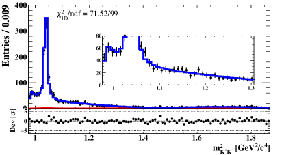
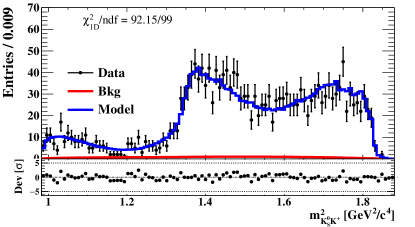
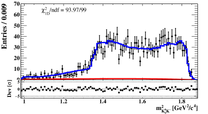
Figure 6: Dalitz plot projections of data sample (full dots) and amplitude model (blue line). Below each projection the deviation between model and data sample is shown in units of its uncertainty. The inset in the first plot shows a zoom on the $K\kern 1.99997pt\overline{\kern-1.99997ptK}{}$ $S$-wave contribution.

Table 7: Result from the Dalitz plot analysis using a model with resonant contributions from $a_{0}(980)^{0}$, $a_{0}(980)^{+}$ and $\phi(1020)$. The first uncertainty is statistical followed by systematic uncertainty. The coupling constant $a_{0}(980)\rightarrow K\kern 1.99997pt\overline{\kern-1.99997ptK}{}$ is determined to be $g_{K\kern 1.39998pt\overline{\kern-1.39998ptK}{}}=($3.47$\pm$0.20$\text{(stat.)}\pm$0.38$\text{(sys.)})$\mathrm{GeV}$$.

Final state Magnitude Phase [$\mathrm{rad}$] Fit fraction [$\mathrm{\char 37\relax}$] $a_{0}(980)^{0}K^{0}_{\scriptscriptstyle S}$ $1$ $0$ $$79$\pm$5$\pm$7$$ $a_{0}(980)^{+}K^{-}$ $$0.67$\pm$0.04$\pm$0.07$$ $$-2.99$^{$0.06$}_{$-0.09$}\pm$0.19$$ $$36$\pm$3$\pm$6$$ $\phi(1020)K^{0}_{\scriptscriptstyle S}$ $$0.78$\pm$0.03$\pm$0.04$$ $$1.84$\pm$0.07$\pm$0.20$$ $$48$\pm$1$\pm$3$$ Total $$163$\pm$11$$

V Branching fraction measurement

The branching fraction of $D^{0}\rightarrow K^{0}_{\scriptscriptstyle S}K^{+}\kern-1.60004ptK^{-}$ is measured using the untagged sample. The branching fraction is given by

$${\mathcal{B}}_{3K}=\frac{N^{3K}}{2N_{D^{0}{\kern-1.12003pt\kern 1.39998pt\overline{\kern-1.39998ptD}\rule{0.0pt}{4.52083pt}{}^{0}}}\cdot f_{QC}\cdot\epsilon_{3K}\cdot{\mathcal{B}}_{K^{0}_{\scriptscriptstyle S}\rightarrow\pi^{+}\pi^{-}}}.$$ (34)

Here, the signal yield is denoted by $N^{3K}$, which is corrected for the efficiency of reconstruction and selection $\epsilon_{3K}$. We correct for the branching fraction of the $K^{0}_{\scriptscriptstyle S}$ reconstruction mode using ${\mathcal{B}}(K^{0}_{\scriptscriptstyle S}\rightarrow\pi^{+}\pi^{-})=$69.20\pm 0.05\text{\,}\mathrm{\char 37\relax}$$ Patrignani et al. (2016). Our branching fraction result is normalized to the number of $D^{0}{\kern-1.60004pt\kern 1.99997pt\overline{\kern-1.99997ptD}\rule{0.0pt}{6.45831pt}{}^{0}}$ decays in the data sample Ablikim et al. (2018):

$$N_{D^{0}{\kern-1.12003pt\kern 1.39998pt\overline{\kern-1.39998ptD}\rule{0.0pt}{4.52083pt}{}^{0}}}=($10\,597$\pm$28$\pm$98$)${\mathrm{\times 10}}^{3}$.$$ (35)

The branching fraction in an untagged $D^{0}{\kern-1.60004pt\kern 1.99997pt\overline{\kern-1.99997ptD}\rule{0.0pt}{6.45831pt}{}^{0}}$ sample is linked to the branching fraction of an isolated $D^{0}$ decay via the correction factor $f_{QC}$ which is derived in the following section.

V.1 Quantum entanglement

We consider a pair of $D^{0}$ mesons, of which one meson decays to the signal final state and the other to an arbitrary final state. In the following, $i$ and $j$ are different final states. The branching fraction is given by

$${\mathcal{B}}_{jX}=\absolutevalue{{\mathcal{M}}_{jX}}^{2} =\sum_{i}\left(\absolutevalue{{\mathcal{M}}_{ji}}^{2}+\absolutevalue{{\mathcal{M}}_{j\overline{\imath}}}^{2}\right)$$

$$=\sum_{i}\left({\mathcal{B}}_{ji}+{\mathcal{B}}_{j\overline{\imath}}\right).$$ (36)

We sum over all possible final states of one $D^{0}$ meson. As mentioned before we use a normalization in which the phase space integral over the norm of an amplitude corresponds to a branching fraction. Using Eq. 9 we find that

$${\mathcal{B}}_{jX} =\sum_{i}\kern 1.99997pt\overline{\kern-1.99997pt{\mathcal{B}}}{}_{j}\kern 1.99997pt\overline{\kern-1.99997pt{\mathcal{B}}}{}_{i}\bigg{[}1+\expectationvalue{r_{i}}+\expectationvalue{r_{j}}+\expectationvalue{r_{i}}\expectationvalue{r_{j}}$$

$$\qquad-\expectationvalue{2\sqrt{r_{i}}\cos\delta_{i}}\expectationvalue{2\sqrt{r_{j}}\cos\delta_{j}}\bigg{]}.$$ (37)

Here, $\expectationvalue{\cdot}$ denotes phase space averaged values. The branching fractions of isolated $D^{0}$ decay sum up to one

$$\sum_{i}\left(\kern 1.99997pt\overline{\kern-1.99997pt{\mathcal{B}}}{}_{i}+{\mathcal{B}}_{i}\right)=\sum_{i}\left(\kern 1.99997pt\overline{\kern-1.99997pt{\mathcal{B}}}{}_{i}+\kern 1.99997pt\overline{\kern-1.99997pt{\mathcal{B}}}{}_{i}\expectationvalue{r_{i}}\right)=1$$ (38)

and the mixing parameter $y$ can be expressed as Asner and Sun (2006)

$$y=2\sum_{i}\kern 1.99997pt\overline{\kern-1.99997pt{\mathcal{B}}}{}_{i}\expectationvalue{\sqrt{r_{i}}\cos\delta_{i}}.$$ (39)

Thus, Eq. 37 gives

$${\mathcal{B}}_{jX}=\kern 1.99997pt\overline{\kern-1.99997pt{\mathcal{B}}}{}_{j}\left[1+\expectationvalue{r_{j}}-\expectationvalue{2\sqrt{r_{j}}\cos\delta_{j}}y\right].$$ (40)

The correction factor that links the branching fraction of a quantum entangled $D^{0}{\kern-1.60004pt\kern 1.99997pt\overline{\kern-1.99997ptD}\rule{0.0pt}{6.45831pt}{}^{0}}$ pair ${\mathcal{B}}_{jX}$ to the branching fraction of an isolated $D^{0}$ decay ${\mathcal{B}}_{j}$ is then given by

$$2f_{QC} =1+\expectationvalue{r_{j}}-y\expectationvalue{2\sqrt{r_{j}}\cos\delta_{j}}.$$ (41)

The quantities $r_{j}$ and $\delta_{j}$ depend on the phase space position, and we use the phase space averaged values for the calculation of $f_{QC}$. From the Dalitz amplitude model a value of $f_{QC}=$1.035\pm 0.015$$ is obtained for the final state $j=K^{0}_{\scriptscriptstyle S}K^{+}\kern-1.60004ptK^{-}$. The statistical uncertainty of the Dalitz amplitude model is propagated to $f_{QC}$ via an MC approach. The limited statistics of the tagged sample cause a rather large uncertainty on $f_{QC}$ of $1.45\text{\,}\mathrm{\char 37\relax}$.

V.2 Systematic uncertainties

Systematic uncertainties on the branching fraction measurement arise from several sources. An overview is given in Table 8.

Deviations between data and MC simulation can lead to different resolutions in specific variables, thus leading to different efficiencies for the selection criteria. Most selection variables are already included in the uncertainty on track reconstruction (see below). For the remaining requirement on the $\chi^{2}$ of the $D^{0}$ vertex fit we find an uncertainty of $0.8\text{\,}\mathrm{\char 37\relax}$. Furthermore, we see a small difference in the $K^{0}_{\scriptscriptstyle S}$ mass resolution and therefore the $K^{0}_{\scriptscriptstyle S}$ width is a free parameter in the fit. The $D^{0}$ mass resolution is consistent between data and MC simulation.

The branching fraction measurement requires the total efficiency for reconstruction and selection which is sensitive to the substructure of the decay. We use the Dalitz plot model to generate signal events which we use for efficiency determination. Since the fit quality of the Dalitz model is excellent we do not assign an additional uncertainty.

The signal yield is determined using models for signal and background. The model shape is determined using MC simulation and discrepancies between data and simulation can therefore lead to a bias in the yield determination. We use the covariance matrix of the fit and a multi-dimensional Gaussian to generate sets of shape parameters and recalculate signal and background yields using these sets of parameters. We find that the systematic uncertainty is less than $0.2\text{\,}\mathrm{\char 37\relax}$. Furthermore, we check that the fit reproduces the correct values.

The systematic uncertainty of the $K^{0}_{\scriptscriptstyle S}$ reconstruction efficiency is studied using ${J\mskip-3.0mu/\mskip-2.0mu\psi\mskip 2.0mu}\rightarrow K^{*\pm}K^{\mp}$ and ${J\mskip-3.0mu/\mskip-2.0mu\psi\mskip 2.0mu}\rightarrow\phi K^{0}_{\scriptscriptstyle S}K^{\mp}\pi^{\pm}$ control samples Ablikim et al. (2015a). We assign an uncertainty of $1.2\text{\,}\mathrm{\char 37\relax}$ for it.

The efficiency for charged track reconstruction and particle identification is studied using hadronic $D\kern 1.99997pt\overline{\kern-1.99997ptD}$ decaysAblikim et al. (2015b). We assign $1\text{\,}\mathrm{\char 37\relax}$ uncertainty per charged kaon track.

The systematic uncertainty, and also the total uncertainty of the measurement is dominated by the contributions due to track reconstruction and particle identification. In total the systematic uncertainty on the branching fraction measurement is $3.5\text{\,}\mathrm{\char 37\relax}$.

V.3 Result

Table 8: Overview of systematic uncertainties.

Systematic uncertainties [$\mathrm{\char 37\relax}$]
Quantum entanglement		$1.45$
Selection		$0.80$
Signal/background model		$0.20$
Efficiency	$K^{0}_{\scriptscriptstyle S}$ reconstruction	$1.20$
	$K^{\pm}$ tracking	$2.00$
	$K^{\pm}$ particle identification	$2.00$
	MC statistics	$0.22$
Ext.	Number of $D^{0}{\kern-1.60004pt\kern 1.99997pt\overline{\kern-1.99997ptD}\rule{0.0pt}{6.45831pt}{}^{0}}$ decays	$1.00$
	$\mathcal{B}$ ($K^{0}_{\scriptscriptstyle S}$ $\rightarrow$ $\pi^{+}$ $\pi^{-}$)	$0.07$
	Total	$3.67$

The signal yield $N^{3K}$ is determined by a two-dimensional fitting procedure. The projections to $m_{bc}$ and $m_{ks}$ of the data sample and the fit model are shown in Fig. 2. We obtain a signal yield of $11\,660\pm 118.$ events. Using the inclusive MC sample we find an efficiency for reconstruction and selection of $\epsilon_{3K}=$17.04\pm 0.04\text{\,}\mathrm{\char 37\relax}$$ where the uncertainty is due to limited MC statistics.

According to Eq. 34 the branching fraction of $D^{0}\rightarrow K^{0}_{\scriptscriptstyle S}K^{+}\kern-1.60004ptK^{-}$ is

$${\mathcal{B}}(D^{0}\rightarrow K^{0}_{\scriptscriptstyle S}K^{+}\kern-1.60004ptK^{-}) =$$ (42)

$$($4.51$\pm$0.05$\text{(stat.)}\pm$0.16$\text{(sys.)})${\mathrm{\times 10}}^{-3}$.$$

The relative statistical and systematic uncertainties are $1.0\text{\,}\mathrm{\char 37\relax}$ and $3.67\text{\,}\mathrm{\char 37\relax}$, respectively. The total uncertainty is $3.81\text{\,}\mathrm{\char 37\relax}$.

VI Conclusion

In summary, we investigate the decay $D^{0}\rightarrow K^{0}_{\scriptscriptstyle S}K^{+}\kern-1.60004ptK^{-}$ using $2.93\text{\,}{\mathrm{fb}}^{-1}$ of $e^{+}e^{-}$ collisions collected at $\sqrt{s}=$3.773\text{\,}\mathrm{GeV}$$ recorded with the BESIII experiment. We analyse the Dalitz plot and measure its branching fraction.

The $K^{0}_{\scriptscriptstyle S}K^{+}\kern-1.60004ptK^{-}$ Dalitz plot is described using an isobar amplitude model. We select the optimal set of resonances using a ‘penalty term’ method and find that the Dalitz plot is well described using an amplitude model with six resonances of $a_{0}(980)^{0}$, $a_{0}(980)^{+}$, $\phi(1020)$, $a_{2}(1320)^{+}$, $a_{2}(1320)^{-}$ and $a_{0}(1450)^{-}$. The largest contribution to the total intensity comes from the $a_{0}(980)^{0}$ that, together with its charged partner, describes the $K\kern 1.99997pt\overline{\kern-1.99997ptK}{}$ threshold. Both resonances show a strong interference which leads to a sum of fit fractions of the Dalitz amplitude model of $176\pm 20.\text{\,}\mathrm{\char 37\relax}$.

The $f_{0}(980)$ could appear as an intermediate resonance, but our strategy for resonance selection does not favor a model that includes the $f_{0}(980)$. With respect to the nominal model its significance is $1.02\text{\,}\sigma$. The $a_{0}(980)$ couples strongly to the channel $K\kern 1.99997pt\overline{\kern-1.99997ptK}{}$ as well as to the channel $\pi\eta$. We measure its coupling to $K\kern 1.99997pt\overline{\kern-1.99997ptK}{}$ to be $g_{K\kern 1.39998pt\overline{\kern-1.39998ptK}{}}=($3.77$\pm$0.24$\pm$0.35$)$\mathrm{GeV}$$; within the uncertainties this is in agreement with previous measurements. For the Dalitz plot analysis, both $D^{0}$ mesons in each event are reconstructed. Therefore the sample size is limited and statistical and systematic uncertainties are of the same order. The result is influenced by the quantum entanglement of $D^{0}$ and $\kern 1.99997pt\overline{\kern-1.99997ptD}\rule{0.0pt}{6.45831pt}{}^{0}$ with respect to the measurements of isolated $D^{0}$ decays. We include this effect in our amplitude models in order to quote parameters of an isolated $D^{0}$ decay. The magnitude and phase of the ratio of $D^{0}$ and $\kern 1.99997pt\overline{\kern-1.99997ptD}\rule{0.0pt}{6.45831pt}{}^{0}$ amplitudes of the tag decays are necessary to describe this effect. Since those are not measured for all tag channels we use the parameters of $D^{0}$ $\rightarrow$ $K^{+}$ $\pi^{-}$ for all channels. The effect of this substitution on the final result is included in the systematic uncertainties.

The model includes the $a_{2}(1320)^{-}$ and the $a_{0}(1450)^{-}$ which are expected to be doubly Cabibbo-suppressed and, therefore, should have a significantly smaller fit fraction than their positively charged partners. The fact that we do not see this could be a hint that those contributions are artefacts of an imperfect model description in parts of the phase space. Those states and the $a_{2}(1320)^{+}$ have a combined statistical significance of $5.9\text{\,}\sigma$. Each of their isospin partners $a_{2}(1320)^{0}$, $a_{0}(1450)^{0}$ and $a_{0}(1450)^{+}$ have a statistical significance of $2.1\text{\,}\sigma$ or less with respect to the nominal model and are not included by our method for resonance selection. Because of the small fit fractions of $a_{2}(1320)^{+}$, $a_{2}(1320)^{-}$ and $a_{0}(1450)^{-}$ we decide to report upper limits. Due to these problems of the model, we additionally quote a model built from the ‘visible’ resonant states $a_{0}(980)^{0}$, $a_{0}(980)^{+}$ and $\phi(1020)$. The result is given in Table 7. In comparison with the result from BABAR Aubert et al. (2005) we use a different set of resonances which leads to stronger interference terms.

We measure the branching fraction of the decay $D^{0}\rightarrow K^{0}_{\scriptscriptstyle S}K^{+}\kern-1.60004ptK^{-}$ to be $($4.51$\pm$0.05$\text{(stat.)}\pm$0.16$\text{(sys.)})${\mathrm{\times 10}}^{-3}$$. This is the first absolute measurement. We use the Dalitz amplitude model to accurately describe the signal decay in simulation and also to obtain the quantum entanglement correction factor. The measurement is in good agreement with previous measurements and we are able to reduce the uncertainty significantly. The measurement is systematically limited.

VII Acknowledgments

The BESIII collaboration thanks the staff of BEPCII and the IHEP computing center for their strong support. This work is supported in part by National Key Basic Research Program of China under Contract No. 2015CB856700; National Natural Science Foundation of China (NSFC) under Contracts Nos. 11625523, 11635010, 11735014, 11822506, 11835012; the Chinese Academy of Sciences (CAS) Large-Scale Scientific Facility Program; Joint Large-Scale Scientific Facility Funds of the NSFC and CAS under Contracts Nos. U1532257, U1532258, U1732263, U1832207; CAS Key Research Program of Frontier Sciences under Contracts Nos. QYZDJ-SSW-SLH003, QYZDJ-SSW-SLH040; 100 Talents Program of CAS; INPAC and Shanghai Key Laboratory for Particle Physics and Cosmology; ERC under Contract No. 758462; German Research Foundation DFG under Contracts Nos. Collaborative Research Center CRC 1044, FOR 2359; Istituto Nazionale di Fisica Nucleare, Italy; Koninklijke Nederlandse Akademie van Wetenschappen (KNAW) under Contract No. 530-4CDP03; Ministry of Development of Turkey under Contract No. DPT2006K-120470; National Science and Technology fund; STFC (United Kingdom); The Knut and Alice Wallenberg Foundation (Sweden) under Contract No. 2016.0157; The Royal Society, UK under Contracts Nos. DH140054, DH160214; The Swedish Research Council; U. S. Department of Energy under Contracts Nos. DE-FG02-05ER41374, DE-SC-0010118, DE-SC-0012069; University of Groningen (RuG) and the Helmholtzzentrum fuer Schwerionenforschung GmbH (GSI), Darmstadt.

References

- Tanabashi et al. (2018) M. Tanabashi et al. (Particle Data Group), Phys. Rev. D98, 030001 (2018).
- Aubert et al. (2008) B. Aubert et al. (BaBar Collaboration), Phys. Rev. D78, 034023 (2008).
- Ablikim et al. (2020a) M. Ablikim et al. (BESIII Collaboration), “Improved model-independent determination of the strong-phase difference between and to decays,” (2020a), to be submitted to PRD.
- Aubert et al. (2005) B. Aubert et al. (BaBar Collaboration), Phys. Rev. D72, 052008 (2005).
- Ablikim et al. (2013) M. Ablikim et al. (BESIII Collaboration), Chin. Phys. C37, 123001 (2013).
- Ablikim et al. (2016) M. Ablikim et al. (BESIII Collaboration), Phys. Lett. B753, 629 (2016).
- Yu et al. (2016) C. Yu et al., in Proceedings, 7th International Particle Accelerator Conference (IPAC 2016): Busan, Korea (2016).
- Ablikim et al. (2020b) M. Ablikim et al. (BESIII Collaboration), Chin. Phys. C44, 040001 (2020b).
- Ablikim et al. (2010) M. Ablikim et al. (BESIII Collaboration), Nucl. Instrum. Meth. A614, 345 (2010).
- Agostinelli et al. (2003) S. Agostinelli et al. (GEANT4), Nucl. Instrum. Meth. A506, 250 (2003).
- Jadach et al. (2001) S. Jadach, B. F. L. Ward, and Z. Was, Phys. Rev. D63, 113009 (2001), arXiv:hep-ph/0006359 [hep-ph] .
- Lange (2001) D. J. Lange, Nucl. Instrum. Meth. A462, 152 (2001).
- Ping (2008) R.-G. Ping, Chin. Phys. C32, 599 (2008).
- Patrignani et al. (2016) C. Patrignani et al. (Particle Data Group), Chin. Phys. C40, 100001 (2016).
- Chen et al. (2000) J. C. Chen, G. S. Huang, X. R. Qi, D. H. Zhang, and Y. S. Zhu, Phys. Rev. D62, 034003 (2000).
- Yang et al. (2014) R.-L. Yang, R.-G. Ping, and H. Chen, Chin. Phys. Lett. 31, 061301 (2014).
- Richter-Was (1993) E. Richter-Was, Phys. Lett. B303, 163 (1993).
- Ablikim et al. (2018) M. Ablikim et al. (BESIII Collaboration), Chin. Phys. C42, 083001 (2018).
- Gaiser (1982) J. E. Gaiser, Charmonium Spectroscopy From Radiative Decays of the and , Ph.D. thesis, SLAC (1982).
- Albrecht et al. (1989) H. Albrecht et al. (ARGUS), Phys. Lett. B229, 304 (1989).
- Michel et al. (2014) M. Michel et al., J. Phys. Conf. Ser. 513, 022025 (2014).
- Fritsch et al. (2019) M. Fritsch, K. Goetzen, W. Gradl, M. Michel, K. Peters, S. Pflüger, A. Pitka, P. Weidenkaff, and J. Zhang, “Compwa: The common partial wave analysis framework,” (2019).
- Libby et al. (2010) J. Libby et al. (CLEO Collaboration), Phys. Rev. D82, 112006 (2010).
- Amhis et al. (2019) Y. S. Amhis et al. (HFLAV), (2019), arXiv:1909.12524 [hep-ex] .
- Evans et al. (2016) T. Evans, S. Harnew, J. Libby, S. Malde, J. Rademacker, and G. Wilkinson, Phys. Lett. B757, 520 (2016), [Erratum: Phys. Lett.B765,402(2017)].
- Asner and Sun (2006) D. M. Asner and W. M. Sun, Phys. Rev. D73, 034024 (2006), [Erratum: Phys. Rev.D77,019901(2008)].
- Blatt and Weisskopf (1979) J. M. Blatt and V. F. Weisskopf, Theoretical Nuclear Physics (Springer, New York, 1979).
- Flatte (1976) S. M. Flatte, Phys. Lett. 63B, 224 (1976).
- Ambrosino et al. (2007) F. Ambrosino et al. (KLOE Collaboration), Eur. Phys. J. C49, 473 (2007).
- Garcia-Martin et al. (2011) R. Garcia-Martin, R. Kaminski, J. R. Pelaez, and J. Ruiz de Elvira, Phys. Rev. Lett. 107, 072001 (2011).
- Ablikim et al. (2005) M. Ablikim et al. (BES Collaboration), Phys. Lett. B607, 243 (2005).
- Teige et al. (1999) S. Teige et al. (E852 Collaboration), Phys. Rev. D59, 012001 (1999).
- Abele et al. (1998) A. Abele et al., Phys. Rev. D57, 3860 (1998).
- Bugg (2008) D. V. Bugg, Phys. Rev. D78, 074023 (2008).
- Ambrosino et al. (2009) F. Ambrosino et al. (KLOE Collaboration), Phys. Lett. B681, 5 (2009).
- Athar et al. (2007) S. B. Athar et al. (CLEO Collaboration), Phys. Rev. D75, 032002 (2007).
- Adams et al. (2011) G. S. Adams et al. (CLEO Collaboration), Phys. Rev. D84, 112009 (2011).
- Vladimirsky et al. (2006) V. V. Vladimirsky et al., Phys. Atom. Nucl. 69, 493 (2006).
- Tibshirani (1996) R. Tibshirani, J. R. Stat. Soc. Ser. B 58, 267 (1996).
- Guegan et al. (2015) B. Guegan, J. Hardin, J. Stevens, and M. Williams, JINST 10, P09002 (2015).
- Schwarz (1978) G. Schwarz, Ann. Stat. 6, 461 (1978).
- Akaike (1974) H. Akaike, IEEE Trans. Autom. Control 19, 716 (1974).
- Aslan and Zech (2005) B. Aslan and G. Zech, Nucl. Instrum. Meth. A 537, 626 (2005).
- Ablikim et al. (2015a) M. Ablikim et al. (BESIII Collaboration), Phys. Rev. D92, 112008 (2015a).
- Ablikim et al. (2015b) M. Ablikim et al. (BESIII Collaboration), Phys. Rev. D92, 072012 (2015b).