Extrapolation for Large-batch Training in Deep Learning

Abstract

Deep learning networks are typically trained by Stochastic Gradient Descent (SGD) methods that iteratively improve the model parameters by estimating a gradient on a very small fraction of the training data. A major roadblock faced when increasing the batch size to a substantial fraction of the training data for improving training time is the persistent degradation in performance (generalization gap). To address this issue, recent work propose to add small perturbations to the model parameters when computing the stochastic gradients and report improved generalization performance due to smoothing effects. However, this approach is poorly understood; it requires often model-specific noise and fine-tuning.
To alleviate these drawbacks, we propose to use instead computationally efficient extrapolation (extragradient) to stabilize the optimization trajectory while still benefiting from smoothing to avoid sharp minima. This principled approach is well grounded from an optimization perspective and we show that a host of variations can be covered in a unified framework that we propose. We prove the convergence of this novel scheme and rigorously evaluate its empirical performance on ResNet, LSTM, and Transformer. We demonstrate that in a variety of experiments the scheme allows scaling to much larger batch sizes than before whilst reaching or surpassing SOTA accuracy.

1 Introduction

The workhorse training algorithm for most machine learning applications—including deep learning—is Stochastic Gradient Descent (SGD). Recently, data parallelism has emerged in deep learning, where large-batch (Goyal et al., 2017) is used to reduce the gradient computation rounds so as to accelerate the training. However, in practice, these large-batch variants suffer from severe issues of test quality loss (Shallue et al., 2018; McCandlish et al., 2018; Golmant et al., 2018), which voids gained computational advantage. While still not completely understood, recent research has linked part of this loss of efficiency to the existence of sharp minima. In contrast, landscapes with flat minima have in empirical studies shown generalization benefits (Keskar et al., 2016; Yao et al., 2018; Lin et al., 2020), though this topic is still actively debated (Dinh et al., 2017).

Another line of research tries to understand general deep learning training from an optimization perspective, in terms of the optimization trajectory in the loss surface (Neyshabur, 2017; Jastrzebski et al., 2020). Golatkar et al. (2019) empirically show that regularization techniques only affect early learning dynamics (initial optimization phase) but matter little in the final phase of training (converging to a local minimum), similar to the critical initial learning phase described in (Achille et al., 2019) and the break-even point analysis on the entire optimization trajectory of Jastrzebski et al. (2020).
These new insights are consistent with empirically developed techniques for the SOTA large-batch training. For example, gradual learning rate warmup for the first few epochs (Goyal et al., 2017; You et al., 2019) is often used; and in local SGD (Lin et al., 2020) for better generalization, stochastic noise injection is only applied after the first phase of training (post-local SGD).

These discussions on optimization and generalization motivate us to answer the following questions when using or developing large-batch techniques for better training: Does the proposed technique improve (initial) optimization, or help to converge to a better local minimum, or both? How and when should we apply the technique?

In this paper, we first revisit the classical smoothing idea (which was recently attributed to avoiding sharp minima in deep learning (Wen et al., 2018; Haruki et al., 2019)) from optimization perspective. We then propose a computational efficient local extragradient method as a way of smoothing for distributed large-batch training, referred to as extrap-SGD; we further extend it to a general framework (extrapolated SGD) for distributed training. We thoroughly evaluate our method on diverse tasks to understand how and when it improves the training in practice. Our empirical results justify the benefits of extrap-SGD, and explain the effects of smoothing ill-conditioned loss landscapes as to exhibit more well-behaved regions, which contain multiple solutions of good generalization properties (Garipov et al., 2018). We show the importance of using extrap-SGD in the critical initial optimization phase, for the later convergence to better local minima; the conjecture is verified by the combination with post-local SGD, which achieves SOTA large-batch training. Our main contributions can be summarized as follows:

• We propose extrap-SGD and extend it to a unified framework (extrapolated SGD) for distributed large-batch training. Extensive empirical results on three benchmarking tasks justify the effects of accelerated optimization and better generalization.

• We provide convergence analysis for methods in the proposed framework, as well as the SOTA large batch training method (i.e. mini-batch SGD with Nesterov momentum). Our analysis explains the large batch optimization inefficiency (diminishing linear speedup) observed in previous empirical work.

2 Related Work

Large-batch training.

The test performance degradation (often denoted as generalization gap) caused by large batch training has recently drawn significant attention (Keskar et al., 2016; Hoffer et al., 2017; Shallue et al., 2018; Masters & Luschi, 2018). Hoffer et al. (2017) argue that the generalization gap in some cases can be closed by increasing training iterations and adjusting the learning rate proportional to the square root of the batch size. Goyal et al. (2017) argue the poor test performance is due to the optimization issue; they try to bridge the generalization gap with the heuristics of linear scale-up of the learning rate during training or during a warmup phase. You et al. (2017) propose Layer-wise Adaptive Rate Scaling (LARS) for better optimization and scaling to larger mini-batch sizes; but the generalization gap does not vanish. Lin et al. (2020) further propose post-local SGD on top of these optimization techniques to inject stochastic noise (to mimic the training dynamics of small batch SGD) during the later training phase.

In addition to the techniques developed for improving optimization and generalization, the optimization ineffectiveness (in terms of required training steps-to-target performance) of large-batch training has been observed. Shallue et al. (2018); McCandlish et al. (2018); Golmant et al. (2018) empirically demonstrate the existence of diminishing linear speedup region across different domains and architectures. Such a limit is also theoretically characterized in (Ma et al., 2017; Yin et al., 2017) for mini-batch SGD in the convex setting.

Smoothing the “sharp minima”.

Some research links generalization performance to flatness of minima. Entropy SGD (Chaudhari et al., 2017) proposes Langevin dynamics in the inner optimizer loop to smoothen out sharp valleys of the loss landscape. From the perspective of large-batch training, Wen et al. (2018) perform “sequential averaging” over models perturbed by isotropic noise, as a way to combat sharp minima. Haruki et al. (2019) claim that injecting different anisotropic stochastic noises on local workers can smoothen sharper minima. However, the claimed “sharper minima” is debatable (Dinh et al., 2017); it is also unclear whether the improved results are due to obtained flatter local minima or improved initial optimization brought by smoothing. We defer detailed discussion to Section 3.2 and 5.2.

Smoothing in classical optimization.

Randomized smoothing has a long history in the optimization literature, see e.g. Nesterov (2011); Duchi et al. (2012); Scaman et al. (2018) which show that a faster convergence rates can be achieved by convolving non-smooth convex functions with Gaussian noise. In contrast to non-smooth convex functions, we focus on the smooth non-convex functions, motivated by deep neural networks.

Extragradient methods and optimization stability.

Another useful building block from optimization is the extragradient method, which is a well-known technique to stabilize the training at each iteration by approximating the implicit update. The method was first introduced in (Korpelevich, 1976) and extended to many variants, e.g. mirror-prox (Nemirovski, 2004), Optimistic Mirror Descent (OMD) (Juditsky et al., 2011) (using past gradient information), extragradient method with Nesterov momentum (Diakonikolas & Orecchia, 2017). Recently its stochastic variants have found new applications in machine learning, e.g., Generative Adversarial Network (GAN) training (Daskalakis et al., 2017; Gidel et al., 2018; Chavdarova et al., 2019; Mishchenko et al., 2019), and low bit model training (Leng et al., 2017).

On the theoretical side, several papers analyze the convergence of stochastic variants of extragradient. Juditsky et al. (2011) study stochastic mirror-prox under restrictive assumptions. Xu et al. (2019) analyze stochastic extragradient in a more general non-convex setting and demonstrate tighter upper bounds than mini-batch SGD, when using mini-batch size $\mathcal{O}(1/\epsilon^{2})$. Mishchenko et al. (2019) revisit and slightly extend the stochastic extragradient for better implicit update approximation. However, their work focuses on min-max GAN training and argues the stochastic extragradient method might not be better than SGD for traditional function minimizations tasks. Our work is the first that combines the idea of Nesterov momentum and extragradient (from past information) for stochastic optimization in the setting of distributed training.

3 Optimization with Extrapolation

Problem Setting and Notation. We consider sum-structured optimization problems of the form $\min_{\mathbf{x}\in\mathbb{R}^{d}}f(\mathbf{x}):=\frac{1}{N}\sum_{i=1}^{N}f_{i}(\mathbf{x})\,,$ where $\mathbf{x}$ denotes the parameters of the model (neural networks in our case), and $f_{i}$ denotes the loss function of the $i$-th (out of $N$) training data examples. To introduce our notation, we recall a standard update of mini-batch SGD at iteration $t$, computed on $K$ devices:

$$\textstyle\mathbf{x}_{t+1}:=\mathbf{x}_{t}-\gamma_{t}\left[\frac{1}{KB}\sum_{k=1}^{K}\sum_{i\in\mathcal{I}^{k}_{t}}\nabla f_{i}(\mathbf{x}_{t})\right]\,.$$ (1)

Here $\mathcal{I}^{k}_{t}$ denotes a subset of the training points selected on device $k$ (typically selected uniformly at random) and we denote by $B:=\left\lvert\mathcal{I}^{k}_{t}\right\rvert$ the local mini-batch size and by $\gamma_{t}$ the step-size (learning rate).

3.1 Accelerated (Stochastic) Local Extragradient for Distributed Training

Motivated by the idea of randomized smoothing in the classic optimization literature (as for reducing the Lipschitz constant of the gradient), we here introduce the novel idea of using extragradient locally, as a way of smoothing loss surface, for efficient distributed large-batch training.

The original idea of extrapolation (or extragradient (Korpelevich, 1976)) was developed to stabilize optimization dynamics on saddle-point problems for a single worker, such as e.g. in GAN training (Gidel et al., 2018; Chavdarova et al., 2019). The idea is to compute the gradient at an extrapolated point, different from the current point from which the update will be performed:

$$\begin{split}\textstyle\mathbf{x}_{t+\frac{1}{2}}=\mathbf{x}_{t}-\gamma\nabla f(\mathbf{x}_{t})\,,\qquad\mathbf{x}_{t+1}=\mathbf{x}_{t}-\gamma\nabla f(\mathbf{x}_{t+\frac{1}{2}})\,.\end{split}$$

This step is intrinsically different from the well-known and widely used accelerated method (i.e. Nesterov momentum):

$$\textstyle\begin{split}\textstyle&\textstyle\mathbf{x}_{t+\frac{1}{2}}=\mathbf{x}_{t}+u\mathbf{v}_{t}\,,\mathbf{v}_{t+1}=u\mathbf{v}_{t}-\gamma\nabla f(\mathbf{x}_{t+\frac{1}{2}})\,,\\ \textstyle&\textstyle\mathbf{x}_{t+1}=\mathbf{x}_{t+\frac{1}{2}}-\gamma\nabla f(\mathbf{x}_{t+\frac{1}{2}})\,,\end{split}$$

where here $1>u\geq 0$ denotes the momentum parameter. The key difference lies in the lookahead step for the gradient computation of these two methods.

Considering different extrapolated local models (with Nesterov momentum) under the distributed training, extrap-SGD combines the effects of randomized smoothing and the stabilized optimization dynamics through extrapolation. Our extrap-SGD follows the idea of extrapolating from the past (currently only used for single worker training (Gidel et al., 2018; Daskalakis et al., 2017)), as a means to avoid additional cost for gradients used to form an extrapolation point. The extrap-SGD method is detailed in Algorithm 1, where the previous local gradients are used for the extrapolation and the superscript $k$ stresses that local models are different. Using the past local mini-batch gradients for extrapolation allows the extrapolation scale $\hat{\gamma}$ to directly take on the learning rate used for small mini-batch training with size $B$, thus avoids the difficulty of hyper-parameter tuning. Note that setting $\hat{\gamma}\!=\!0$ in Algorithm 1 recovers the SOTA large batch training method, i.e., mini-batch SGD with Nesterov momentum.

To the best of our knowledge, it is the first time such an extragradient method is used locally with Nesterov Momentum under the framework of smoothing, for accelerated and smoothed distributed optimization.

Algorithm 1 extrap-SGD

0:  learning rate $\gamma$, inner learning rate $\hat{\gamma}$, momentum factor $u$, initial parameter $\mathbf{x}_{0}$, initial moment vector $\mathbf{v}_{0}\!=\!0$, time step $t\!=\!0$, worker index $k$.

1:  while $\mathbf{x}_{t}$ not converged do

2:    $\mathbf{x}_{t+\frac{1}{4}}^{k}=\mathbf{x}_{t}-\frac{\hat{\gamma}}{B}\sum_{i\in\mathcal{I}^{k}_{t}}\nabla f_{i}(\mathbf{x}_{t-\frac{1}{2}}^{k})$ $\triangleright$ extrapolation step

3:    $\mathbf{x}_{t+\frac{1}{2}}^{k}=\mathbf{x}_{t+\frac{1}{4}}^{k}+u\mathbf{v}_{t}$ $\triangleright$ Nesterov momentum

4:    $\mathbf{v}_{t+1}=u\mathbf{v}_{t}-\frac{\gamma}{KB}\sum_{k,i\in\mathcal{I}^{k}_{t}}\nabla f_{i}(\mathbf{x}_{t+\frac{1}{2}}^{k})$ $\triangleright$ update buffer

5:    $\mathbf{x}_{t+1}=\mathbf{x}_{t}+\mathbf{v}_{t+1}$ $\triangleright$ actual update

6:  end while

6:  $\mathbf{x}_{t}$.

3.2 Unified Extrapolation Framework

Our Algorithm 1 can be extended to a more general extrapolation framework for distributed training, by using diverse extrapolation choices $\mathbf{\zeta}_{t}^{k}$. It is achieved by replacing line 2 in Algorithm 1 by $\mathbf{x}_{t+\frac{1}{4}}^{k}\!=\!\mathbf{x}_{t}-\hat{\gamma}\mathbf{\zeta}_{t}^{k}$. We denote our framework as extrapolated SGD, covering different choices of noise $\mathbf{\zeta}_{t}^{k}$ (e.g. Gaussian noise, uniform noise, and stochastic gradient noise) and extrap-SGD (past mini-batch gradients). We detail some choices of $\mathbf{\zeta}_{t}^{k}$ below and use them as our close baselines for extrap-SGD:

• $\mathbf{\zeta}_{t}^{k}$ as a form of isotropic noise. The noise can be sampled from e.g. an isotropic Gaussian or uniform distribution. Following the idea of Li et al. (2017), the strength of noises added to a filter can be linearly scaled by the $l_{2}$ norm of the filter, instead of fixing a constant perturbation strength over different layers. Formally, the scaled noise $\mathbf{\zeta}^{k}_{t}$ of $j$-th filter at layer $i$ on worker $k$ follows $\left\lVert\mathbf{x}_{t,i,j}\right\rVert\cdot\hat{\mathbf{\zeta}}^{k}_{t,i,j}/\bigl{\|}\hat{\mathbf{\zeta}}^{k}_{t,i,j}\bigr{\|}$. A similar idea was proposed in SmoothOut (Wen et al., 2018), corresponding to letting $\mathbf{\zeta}^{k}_{t}:=\mathbf{\zeta}_{t}$ in our framework.

• $\mathbf{\zeta}_{t}^{k}$ as a form of anisotropic noise. Kleinberg et al. (2018) interpret sequential SGD updates as GD with stochastic gradient noise convolution over update steps. This motivates to use stochastic gradient noise for smoothing (similarly proposed in Haruki et al. (2019)), thus $\mathbf{\zeta}_{t}^{k}$ can be chosen as:

  $$\textstyle\frac{1}{B}\sum_{i\in\mathcal{I}^{k}_{t}}\nabla f_{i}(\mathbf{x}_{t-\frac{1}{2}}^{k})-\frac{1}{KB}\sum_{k}\sum_{i\in\mathcal{I}^{k}_{t}}\nabla f_{i}(\mathbf{x}_{t-\frac{1}{2}}^{k})\,.$$

The side effects of these noise extrapolation variants are the training setup sensitivity, causing the hyperparameter tuning difficulty and limited practical applications. For example, the isotropic noise requires to manually design the noise distribution for each model and dataset; the anisotropic noise distribution will be dynamically varied by different choices of the number of workers, the local mini-batch size, and the objective of the learning task (Zhang et al., 2019).

Despite the existence of variants (Wen et al., 2018; Haruki et al., 2019) and their reported empirical results, none of them has analyzed their convergence behaviors. In the next section, we provide rigorous convergence analysis for our algorithm for distributed training (illustrated in Algorithm 1, which also includes the SOTA practical training algorithm). In Section 5, we empirically evaluate all related methods to better understand the benefits of using extrapolation with smoothing for distributed large-batch training.

4 Theoretical Analysis of Nesterov Momentum and extrap-SGD

We now turn to the theoretical convergence analysis, i.e. we derive an upper bound on the number of iterations to find an approximate solution with small gradient norm.

Following the convention in distributed stochastic optimization, We denote by $f^{\star}$ a lower bound on the values of $f(\mathbf{x})$ and use the following assumptions:

Assumption 1 (Unbiased Stochastic Gradients).

$\forall i\in[N],t\in[T]$, it holds ${\mathbb{E}}\left[\nabla f_{i}(\mathbf{x}_{t})\right]=\nabla f(\mathbf{x}_{t})$.

Assumption 2 (Bounded Gradient Variance).

$\exists\sigma^{2}>0,\forall i\in[N],t\in[T]$, s.t. ${\mathbb{E}}\left[\left\lVert\nabla f_{i}(\mathbf{x}_{t})-\nabla f(\mathbf{x}_{t})\right\rVert^{2}\right]\leq\sigma^{2}$.

Here $\sigma^{2}$ quantifies the variance of stochastic gradients at each local worker and we assume workers access IID training dataset (e.g., data center setting).

Assumption 3 (Lipschitz Gradient).

$\exists L>0$, s.t. $\forall\mathbf{x},\mathbf{y}\in\mathbb{R}^{d},i\in[N]$, the objective function $f_{i}:\mathbb{R}^{d}\rightarrow\mathbb{R}$ satisfies the following condition $\left\lVert\nabla f_{i}(\mathbf{x})-\nabla f_{i}(\mathbf{y})\right\rVert\leq L\left\lVert\mathbf{x}-\mathbf{y}\right\rVert$.

4.1 Analysis for Mini-batch SGD (with Nesterov Momentum)

In this section we first recall the known convergence guarantees for mini-batch SGD (without momentum) on non-convex functions for later reference, and then derive new guarantees for mini-batch SGD with Nesterov momentum.

Theorem 4.1 (Convergence of stochastic distributed mini-batch SGD for non-convex functions (Ghadimi & Lan, 2016)).

Under Assumptions 1–3, after $T$ mini-batch gradient updates, each using $KB$ samples, the mini-batch SGD returns an iterate $\mathbf{x}$ satisfying

$$\textstyle{\mathbb{E}}\left[\left\lVert\nabla f(\mathbf{x})\right\rVert^{2}\right]\leq\mathcal{O}\left(\frac{L\left(f(\mathbf{x}_{0})-f^{\star}\right)}{T}+\frac{\sigma\sqrt{L\left(f(\mathbf{x}_{0})-f^{\star}\right)}}{\sqrt{KBT}}\right)\,.$$

The second term in the rate is asymptotically dominant as long as $KB\!=\!\mathcal{O}\bigl{(}\frac{\sigma^{2}T}{L\left(f(\mathbf{x}_{0})-f^{\star}\right)}\bigr{)}$. In this regime, increasing the mini-batch size gives a linear speedup, as $T\!=\!\mathcal{O}\bigl{(}\frac{\sigma^{2}L\left(f(\mathbf{x})-f^{\star}\right)}{KB\epsilon^{2}}\bigr{)}$ decreases in $KB$, as similarly pointed out by Wang & Srebro (2017). However, when we increase the mini-batch size beyond this critical point, the first term dominates the rate and increasing the mini-batch size further will have less impact on the convergence. This phenomenon has also been empirically verified in deep learning applications (Shallue et al., 2018).

In practice, mini-batch SGD with Nesterov momentum (Nesterov, 1983) is the state-of-the-art deep learning training scheme. However, previous theoretical analysis normally relies on the strong assumption of the bounded mini-batch gradients (Yan et al., 2018). Here we provide a better convergence analysis without such an assumption for distributed mini-batch SGD with Nesterov momentum following closely Yu et al. (2019). The convergence rate is detailed in Theorem 4.2, and for the proof details we refer to Section A of Appendix I.

Theorem 4.2 (Convergence of mini-batch SGD with Nesterov momentum for non-convex functions).

Under Assumption 1–3, for mini-batch SGD with Nesterov momentum, i.e., $\mathbf{x}_{t+\frac{1}{2}}\!=\!\mathbf{x}_{t}+u\mathbf{v}_{t}$, $\mathbf{v}_{t+1}\!=\!u\mathbf{v}_{t}-\frac{\gamma}{KB}\sum_{k=1}^{K}\sum_{i\in\mathcal{I}_{t}^{k}}\nabla f_{i}(\mathbf{x}_{t+\frac{1}{2}})$, $\mathbf{x}_{t+1}\!=\!\mathbf{x}_{t}+\mathbf{v}_{t+1}$, we can show that for optimally tuned stepsize (cf. Lemma A.4) $\gamma\leq\frac{2(1-u)^{2}}{L(u^{3}+1)}$, it holds

$$\textstyle\begin{split}\textstyle{\mathbb{E}}\left[\left\lVert\nabla f(\mathbf{x})\right\rVert^{2}\right]=\mathcal{O}\left(\frac{Lr_{0}(u^{3}+1)}{T(1-u)}+\sqrt{\frac{2Lr_{0}\sigma^{2}}{KBT(1-u)}}\right)\,,\end{split}$$

where here $\mathbf{x}$ denotes a uniformly at random selected $\mathbf{x}_{t+\frac{1}{2}}$ iterate, i.e. $\frac{1}{T}\sum_{t=0}^{T-1}\bigl{\|}\nabla f(\mathbf{x}_{t+\frac{1}{2}})\bigr{\|}^{2}$, and $r_{0}:=f(\mathbf{x}_{0})-f^{\star}$.

The second term is asymptotically dominant as long as $KB=\mathcal{O}\left(\frac{(1-u)}{(u^{3}+1)^{2}}\frac{\sigma^{2}T}{L(f(\mathbf{x}_{0})-f^{\star})}\right)$ and for small $K$ we can achieve the linear speedup where $T=\mathcal{O}\left(\frac{L\sigma^{2}(f(\mathbf{x}_{0})-f^{\star})}{(1-u)KB\epsilon^{2}}\right)$.

Remark 4.3.

Yu et al. (2019) argue that a linear speedup $\mathcal{O}(1/\sqrt{KT})$ for SGD with the local Nesterov momentumcan be achieved. However, this claim is only valid for large $T$ and stepsize $\gamma=\sqrt{K/T}$, cf. (Yu et al., 2019, Cor. 1). We here tune the stepsize differently and show a tighter bound that holds for all $T$, providing a better critical mini-batch size analysis (diminishing linear speedup in terms of optimization) for mini-batch SGD with Nesterov momentum (Shallue et al., 2018).

4.2 Convergence of extrap-SGD

In this subsection, we show the convergence analysis for our novel extrap-SGD for non-convex functions. We also include the analysis for other noise variants of extrapolated SGD, which explains their potential limitations. The proof details can be found in the Section B of Appendix I.

Theorem 4.4 (Convergence of extrap-SGD for non-convex functions).

Under Assumption 1–3, and by defining $\bar{\mathbf{x}}_{t+\frac{1}{2}}:=\frac{1}{K}\sum_{k=1}\mathbf{x}^{k}_{t+\frac{1}{2}}$, it holds for $\hat{\gamma}\leq\frac{u^{2}}{(1-u)^{2}}\gamma$ and $\gamma\leq\frac{(1-u)^{2}}{L(1+3u+u^{3})}$:

$$\textstyle\begin{split}\textstyle&\textstyle{\mathbb{E}}{\frac{1}{T}\sum_{t=0}^{T-1}\left\lVert\nabla f(\bar{\mathbf{x}}_{t+\frac{1}{2}})\right\rVert^{2}}\\ \textstyle&\textstyle\leq\frac{2(1-u)}{\gamma T}{\mathbb{E}}\left[f(\bar{\mathbf{x}}_{0})-f^{\star}\right]+\left(\frac{4\hat{\gamma}^{2}L^{2}}{B}+\frac{\gamma L(1+3u)}{(1-u)^{2}BK}\right)\sigma^{2}\,.\end{split}$$

Remark 4.5.

Using past local gradients for extrapolation in extrap-SGD allows us to directly set $\hat{\gamma}\approx\frac{\gamma}{K}$ for extrap-SGD, where the constraint of $\hat{\gamma}\leq\frac{u^{2}}{(1-u)^{2}}\gamma$ is normally satisfied.

Corollary 4.6.

Considering Theorem 4.4 and tuning the stepsize as in Lemma A.4, with $\gamma\leq\frac{(1-u)^{2}}{L(1+3u+u^{3})}$ and $\hat{\gamma}\leq\frac{\gamma}{K}$, and $r_{0}:=f(\mathbf{x}_{0})-f^{\star}$, we can rewrite the convergence rate of Theorem 4.4 as $\textstyle\begin{split}\textstyle&\textstyle{\mathbb{E}}\left[\frac{1}{T}\sum_{t=0}^{T-1}\left\lVert\nabla f(\bar{\mathbf{x}}_{t+\frac{1}{2}})\right\rVert^{2}\right]\\ \textstyle&\textstyle=\mathcal{O}\left(4(u^{3}+3u+1)\frac{Lr_{0}}{T(1-u)}+2\sqrt{\frac{(19u+1)}{(u^{3}+3u+1)}\frac{2Lr_{0}\sigma^{2}}{KBT(1-u)}}\right)\,.\end{split}$

The second term is asymptotically dominant as long as $KB=\mathcal{O}\bigl{(}\frac{(19u+1)(1-u)}{(u^{3}+3u+1)^{3}}\frac{\sigma^{2}T}{L(f(\mathbf{x}_{0})-f^{\star})}\bigr{)}$ and for small $K$ we can achieve the linear speedup where $T=\mathcal{O}\left(\frac{L\sigma^{2}(f(\mathbf{x}_{0})-f^{\star})}{KB\epsilon^{2}}\frac{19u+1}{(u^{3}+3u+1)(1-u)}\right)$,

Remark 4.7.

By setting $u=0$, we recover the same rates for extrap-SGD in non-convex cases (Theorem 4.2 and Corollary 4.6) as for standard mini-batch SGD (Theorem 4.1) but we cannot show an actual speedup over mini-batch SGD by setting $u>0$. However, thus might not necessarily be a limitation of our approach as to the best of our knowledge, there exist so far no theoretical results for stochastic momentum methods that can show a speedup over mini-batch SGD.

The analysis below extends the proof of extrap-SGD to the other cases of our extrapolated SGD framework.

Theorem 4.8.

Under the extrapolation framework, IID random noise $\zeta_{t}^{k}$ (instead of the past local mini-batch gradients in Algorithm 1) is used for the local extrapolation, where ${\mathbb{E}}\left[\mathbf{\zeta}_{t}^{k}\right]=0$ and ${\mathbb{E}}\left[\left\lVert\mathbf{\zeta}_{t}^{k}\right\rVert^{2}\right]\leq\hat{\sigma}^{2}$. Under Assumption 1–3, it holds for $\gamma\leq\frac{(1-u)^{2}}{L(1+u+u^{3})}$:

$$\textstyle\begin{split}\textstyle&\textstyle{\mathbb{E}}{\frac{1}{T}\sum_{t=0}^{T-1}\left\lVert\nabla f(\bar{\mathbf{x}}_{t+\frac{1}{2}})\right\rVert^{2}}\leq\frac{2(1-u)}{\gamma T}{\mathbb{E}}\left[f(\bar{\mathbf{y}}_{0})-f(\bar{\mathbf{y}}_{T})\right]\\ \textstyle&\textstyle\qquad+\frac{\gamma L(1+u)}{(1-u)^{2}BK}\sigma^{2}+(L^{2}+\frac{(1-u)^{2}L}{\gamma u^{3}K})2\hat{\gamma}^{2}T\hat{\sigma}^{2}\,.\end{split}$$

Remark 4.9.

The choice of using random noise for extrapolation in Theorem 4.8 requires the manual introduction of the noise distribution ($\hat{\sigma}^{2}$) for each problem setup. The dependence on the unknown relationship between $\hat{\sigma}^{2}$ and $\sigma^{2}$ results in the difficulty of providing a concise convergence analysis (e.g. exact convergence rate, the critical mini-batch size) for Theorem 4.8.

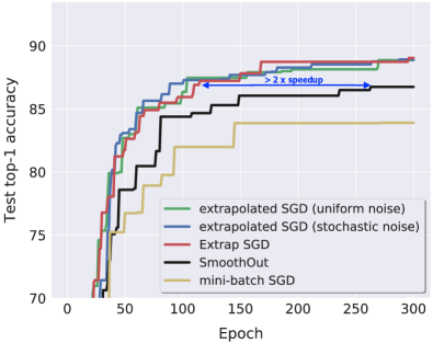
(a) Learning curves for different methods (w/o learning rate decay).

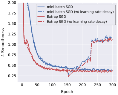
(b) Better smoothness of extrap-SGD.

Figure 1: Understanding the learning behaviors of different methods on the large-batch training (with mini-batch size $8,192$ on $32$ workers) for training ResNet-20 on CIFAR-10. The visualization of smoothness in Figure 1(b) follows the idea in (Santurkar et al., 2018; Haruki et al., 2019); it takes $8$ additionally steps (each with $30\%$ of the update) in the direction of the update for each training step, and the smoothness of a training step is expressed by the maximum value of $L$ (evaluated after local update steps) satisfying the Assumption 3. We use the learning rate scaling and warmup in Goyal et al. (2017) for the first $5$ epochs, and $\gamma$ and $\tilde{\gamma}$ are fine-tuned for different methods.

5 Experiments

We first briefly outline the general experimental setup below (for more details refer to Appendix C) and then thoroughly evaluate our framework on different challenging large-batch training tasks. We aim to challenge and push the limit of large-batch training. We limit our attention to three standard and representative benchmarking tasks, with a controlled epoch budget (for each task). We ensure the used mini-batch size is a significant fraction of the whole dataset. Performing experiments on a much larger dataset for the same demonstration purposes is out of our computational ability.

5.1 Experimental Setup

Datasets.

We evaluate all methods on the following three tasks: (1) Image Classification for CIFAR-10/100 (Krizhevsky & Hinton, 2009) ($50$K training samples and $10$K testing samples with $10/100$ classes) with the standard data augmentation and preprocessing scheme (He et al., 2016; Huang et al., 2016b); (2) Language Modeling for WikiText2 (Merity et al., 2016) (the vocabulary size is $33$K, and its train and validation set have $2$ million tokens and $217$K tokens respectively); and (3) Neural Machine Translation for Multi30k (Elliott et al., 2016).

Models and training schemes.

Several benchmarking models are used in our experimental evaluation. (1) ResNet-20 (He et al., 2016) and VGG-11 (Simonyan & Zisserman, 2014) on CIFAR for image classification, (2) two-layer LSTM (Merity et al., 2017) with hidden dimension of size $128$ on WikiText-2 for language modeling, and (3) a down-scaled transformer (factor of $2$ w.r.t.< the base model in Vaswani et al. (2017)) for neural machine translation. Weight initialization schemes for the three tasks follow Goyal et al. (2017); He et al. (2015), Merity et al. (2017) and Vaswani et al. (2017) respectively.

We use mini-batch SGD with a Nesterov momentum of $0.9$ without dampening for image classification and language modeling tasks, and Adam for neural machine translation tasks. In the following experiment section, the term “mini-batch SGD” indicates the mini-batch SGD with Nesterov momentum unless mentioned otherwise.

For experiments on image classification and language modeling, unless mentioned otherwise the models are trained for $300$ epochs; the local mini-batch sizes are set to $256$ and $64$ respectively. By default, all related experiments will use learning rate scaling and warmup scheme (Goyal et al., 2017; Hoffer et al., 2017). The learning rate is always gradually warmed up from a relatively small value for the first few epochs. Besides, the learning rate $\gamma$ in image classification task will be dropped by a factor of $10$ when the model has accessed $50\%$ and $75\%$ of the total number of training samples (He et al., 2016; Huang et al., 2016a). The LARS is only applied on image classification task (You et al., 2017).

For experiments on neural machine translation, we use standard inverse square root learning rate schedule (Vaswani et al., 2017). The warmup step is set to $4000$ for the mini-batch size of $64$ and will be linearly scaled down by the global mini-batch size.

We carefully tune the learning rate $\gamma$ and the trust term $\tilde{\gamma}$ in You et al. (2017). The tuning procedure ensures that the best hyper-parameter lies in the middle of our search grids; otherwise, we extend our search grid. The procedure of hyperparameter tuning can be found in Appendix C.1.

5.2 Evaluation on Large-batch Training

Superior performance of extrap-SGD on different tasks.

We evaluate our extrapolation framework and compare it with SOTA large-batch training methods on CIFAR-10 image classification (Figure 1) and WikiText2 language modeling (Figure 2). To better exhibit the optimization behaviors of different methods, for these two tasks we do not decay the learning rate. The extrapolated SGD framework in general significantly accelerates the optimization and leads to better test performance than the existing SOTA methods. For example, the smaller gradient Lipschitz constant illustrated in Figure 1(b) demonstrates the improved optimization landscape, which explains the at least $2\times$ speedup in terms of the convergence (after thorough hyperparameter tuning) in Figure 1(a) and Figure 2.

We further extend the extrapolation idea of extrap-SGD to extrap-Adam and validate its effectiveness (compared with Adam) on neural machine translation with Transformer. The algorithmic description refers to Algorithm 3 in Appendix D.2. Figure 3 shows the results of large-batch training (using $4\%$ and $16\%$ of the training data per mini-batch) and extrap-Adam again outperforms the Adam with at least $2\times$ speedup.

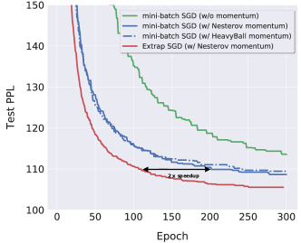
	$K\!=\!24$	$K\!=\!48$
mini-batch SGD	$108.39\pm 0.31$	$110.16\pm 0.67$
extrap-SGD	$105.86\pm 0.32$	$107.86\pm 0.50$

Figure 2: The perplexity (PPL, the lower the better) of training WikiText-2 on LSTM. The global mini-batch size are $1{,}536$ and $3{,}072$ for $K\!=\!24$ and $K\!=\!48$ respectively, accounting for $2\%$ and $4\%$ of the total training data. We use the learning rate scaling and warmup in Goyal et al. (2017), and use constant learning rate after the warmup. We finetune the $\gamma$ for mini-batch SGD (and its momentum variants); extrap-SGD reuses the hyper-parameter from mini-batch SGD. The results of the inline table are averaged over three different seeds. The displayed learning curves are based on $K\!=\!24$ and more details refer to Appendix E.2.

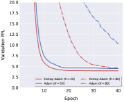
(a) Perplexity (validation).

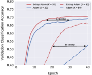
(b) Accuracy (validation).

Figure 3: Training extrap-Adam on Transformer for Multi30k. The evaluations are performed on the validation dataset, for the training on $K\!=\!20$ and $K\!=\!80$ workers (corresponding to roughly $4\%$ and $16\%$ of the total training data). We use the standard inverse square root learning rate schedule (Vaswani et al., 2017) and scale the warmup step based on the number of workers.

Table 1: The performance comparison of different methods for large-batch training on CIFAR-10 (mini-batch of size $8{,}192$ on $K\!=\!32$). Two neural architectures (ResNet-20 and VGG-11) are considered (with and without batch normalization). Unless mentioned otherwise each method will use the learning rate scaling and warmup in Goyal et al. (2017) and LARS in You et al. (2017). We finetune $\gamma$ and $\tilde{\gamma}$ for mini-batch SGD and SmoothOut (with $\hat{\gamma}$ additionally). For the results of extrapolated SGD, we reuse the optimal $\gamma$ and $\tilde{\gamma}$ tuned on mini-batch SGD; $\hat{\gamma}$ is fine-tuned for noise-based extrapolation variants. The results are averaged over three different seeds.

	mini-batch SGD (w/o LARS)	extrap-SGD (w/o LARS)	mini-batch SGD	SmoothOut (Wen et al., 2018)	extrapolated SGD, uniform noise	extrapolated SGD, stochastic noise	extrap-SGD
ResNet-20 on CIFAR-10	$90.00\pm 0.48$	$90.47\pm 0.16$	$91.36\pm 0.19$	$91.55\pm 0.20$	$91.53\pm 0.25$	$91.66\pm 0.24$	$91.72\pm 0.11$
VGG-11 on CIFAR-10	$73.09\pm 9.35$	$76.79\pm 3.5$	$86.64\pm 0.10$	$86.92\pm 0.15$	$87.00\pm 0.31$	$86.04\pm 0.43$	$87.00\pm 0.26$

Optimization v.s. Generalization benefits.

To better understand when and how extrap-SGD (and extrapolated SGD) help, we switch our attention to the commonly accepted training practices: using an initial large learning rate and decaying when the training plateaus. The common beliefs (LeCun et al., 1991; Kleinberg et al., 2018) argue that, the initial large learning rate accelerates the transition from random initialization to convergence regions (optimization), and the decaying leads the convergence to local minimum (generalization).

Table 1 thoroughly evaluates the large-batch training performance (ResNet-20 on CIFAR-10 for mini-batch size $8{,}192$, with learning rate decay schedule) for all related methods. Though the remarkable optimization improvements in Figure 1(a) justify the effects of extrap-SGD (and extrapolated SGD), i.e. smooth the ill-conditioned loss landscape, decaying the learning rate diminishes our advantages, as illustrated in Table 1 and Figure 5 in Appendix. We argue that extrap-SGD and its variants can smoothen the loss surface thus avoid some bad local minima regions, but it cannot guarantee to converge to a much better local minimum, contrary to the statements in (Wen et al., 2018; Haruki et al., 2019). They use (limited) empirical generalization metrics as the main arguments of the “flatter minima”, ignoring the complex training dynamics; their ignored SOTA optimization techniques (e.g. LARS in some experiments) might also result in the improper understandings. Our empirical results provide insights: the primary benefits of extrap-SGD are on the optimization phase (early training phase) and will diminish in the later training phase. It is also reflected in Figure 1(b) in terms of the smoothness.

Combining extrap-SGD with post-local SGD.

Given our new insights in the previous paragraph, here we try to understand the importance of better optimization brought by extrap-SGD for the eventual generalization. We consider the post-local SGD in Lin et al. (2020), a known technique arguing to converge to flatter local minimum for better generalization. This choice comes from the noticeable optimization benefits of extrap-SGD in the initial training phase while post-local SGD targeting to converge to “flatter minima” for the later training phase. Please refer to Algorithm 2 in Appendix D.1 for training details.

We argue that extrap-SGD biases the optimization trajectory towards a better-conditioned loss surface, where solutions with good generalization properties can be found more easily. Figure 4 challenges the extreme large-batch training (mini-batch of size $16{,}384$ on $64$ workers, accounting for $33\%$ of training data) for ResNet-20 on CIFAR-10 with different epoch budgets. We can notice that the improper optimization in the critical initial learning phase of the mini-batch SGD results in a significant generalization gap, which cannot be addressed by adding post-local SGD or increasing the number of training epochs alone. extrap-SGD, on the contrary, avoids the regions containing bad local minima, complementing the ability of post-local SGD for converging to better solutions. Table 2 in the Appendix E.1 additionally reports a similar observation for mini-batch of size $8{,}192$ on more datasets.

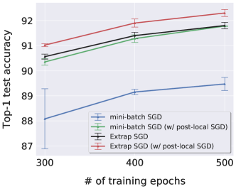
Figure 4: The test top-1 accuracy of integrating extrap-SGD with post-local SGD (Lin et al., 2020). The performance of ResNet-20 on CIFAR-10/100 is evaluated with a global mini-batch size of $16,384$ ($33\%$ of the total training data with $64$ workers). By default we use the learning rate scaling and warmup in Goyal et al. (2017) and LARS in You et al. (2017). We individually finetune $\gamma$ and $\tilde{\gamma}$ for each base method; the local update step $H$ is tuned and set to $H\!=\!4$. The learning rate is decayed by $10$ when the model has accessed $50\%$ and $75\%$ of the total training samples. The results are averaged over three different seeds.

5.3 Ablation study

extrap-SGD for different local mini-batch sizes and number of workers.

Table 3 in the Appendix E.1 evaluates how different combinations of the local mini-batch size and the number of workers will impact the performance, for a given global mini-batch size ($8{,}192$ for ResNet-20 on CIFAR-10). The benefits of extrap-SGD can be further pronounced when increasing the number of workers, which is the common practice for large-batch training. Similar observation can be found in Figure 3 for the increased number of workers (as well as the global mini-batch size).

Understanding the effect of momentum.

Given the mixed effects of local extrapolation and momentum acceleration in extrap-SGD, Figure 7 in Appendix E.3 decouples these two factors for the training ResNet-20 on CIFAR-10 with mini-batch of size $8{,}192$. We can witness that (1) extrap-SGD can take advantages of both extragradient as well as the acceleration from the momentum, and thus can always be applied for accelerated and stabilized distributed optimization; (2) using extrapolation alone (no momentum) in extrap-SGD still outperforms mini-batch SGD with tuned momentum factor; (3) tuning momentum factor for mini-batch SGD can marginally improve the optimization performance but cannot eliminate the optimization difficulty.

6 Conclusion

In this work, we adopt the idea of randomized smoothing to distributed training and propose extrap-SGD to perform extrapolation with past local mini-batch gradients. The idea further extends to a unified framework, covering multiple noise extrapolation variants. We provide convergence guarantees for methods within this framework, and empirically justify the remarkable benefits of our methods on image classification, language modeling and neural machine translation tasks. We further investigate and understand the properties of our methods; the algorithms smoothen the ill-conditioned loss landscape for faster optimization and biases the optimization trajectory to well-conditioned regions. These insights further motivate us to combine our methods with post-local SGD for SOTA large-batch training.

Part I Omitted proof for the convergence analysis

Appendix A Nonconvex proof for Nesterov Momentum

One iterate of SGD with Nesterov momentum can be expressed as follows:

$$\begin{split}\mathbf{x}_{t+\frac{1}{2}}&=\mathbf{x}_{t}+u\mathbf{v}_{t}\,,\qquad\mathbf{v}_{t+1}=u\mathbf{v}_{t}-\frac{\gamma}{BK}\sum_{k=1}^{K}\sum_{i\in\mathcal{I}_{t}^{k}}\nabla f_{i}(\mathbf{x}_{t+\frac{1}{2}})\,,\qquad\mathbf{x}_{t+1}=\mathbf{x}_{t}+\mathbf{v}_{t+1}\,,\end{split}$$ (2)

where $\mathbf{v}_{0}=0$. In the rest of Section A, we use $\mathbf{g}_{t}:=\frac{1}{KB}\sum_{k=1}^{K}\sum_{i\in\mathcal{I}_{t}^{k}}\nabla f_{i}(\mathbf{x}_{t})$ to simplify notation. With this simplication the iterate (2) can be expressed as follows:

$$\begin{split}\mathbf{x}_{t+\frac{1}{2}}&=\mathbf{x}_{t}+u\mathbf{v}_{t}\,,\qquad\mathbf{v}_{t+1}=u\mathbf{v}_{t}-\gamma\mathbf{g}_{t+\frac{1}{2}}\,,\qquad\mathbf{x}_{t+1}=\mathbf{x}_{t}+\mathbf{v}_{t+1}\,,\end{split}$$ (3)

We follow the idea of Yu et al. (2019) and define an auxiliary sequence $\bar{\mathbf{y}}_{t}$ for (3):

$$\bar{\mathbf{y}}_{t}=\left\{\begin{array}[]{ll}\mathbf{x}_{\frac{1}{2}}=\mathbf{x}_{0}&\textrm{if $t=0$}\\ \frac{1}{1-u}\mathbf{x}_{t+\frac{1}{2}}-\frac{u}{1-u}\mathbf{x}_{t-\frac{1}{2}}+\frac{\gamma u}{1-u}\mathbf{g}_{t-\frac{1}{2}}&\textrm{if $t\geq 1$}\end{array}\right.\,.$$ (6)

We have the following two auxiliary lemmas:

Lemma A.1.

Consider the sequence $\{\bar{\mathbf{y}}\}$ in (6) and for all $t\geq 0$, we have $\bar{\mathbf{y}}_{t+1}-\bar{\mathbf{y}}_{t}=-\frac{\gamma}{1-u}\mathbf{g}_{t+\frac{1}{2}}$.

Proof.

For the case $t=0$, we have

$$\begin{split}\bar{\mathbf{y}}_{t+1}-\bar{\mathbf{y}}_{t}&=\bar{\mathbf{y}}_{1}-\bar{\mathbf{y}}_{0}\\ &=\frac{1}{1-u}\mathbf{x}_{\frac{3}{2}}-\frac{u}{1-u}\mathbf{x}_{\frac{1}{2}}+\frac{\gamma u}{1-u}\mathbf{g}_{\frac{1}{2}}-\mathbf{x}_{\frac{1}{2}}\\ &=\frac{1}{1-u}(\mathbf{x}_{\frac{3}{2}}-\mathbf{x}_{\frac{1}{2}})+\frac{\gamma u}{1-u}\mathbf{g}_{\frac{1}{2}}\\ &=\frac{1}{1-u}(u\mathbf{v}_{1}-\gamma\mathbf{g}_{\frac{1}{2}})+\frac{\gamma u}{1-u}\mathbf{g}_{\frac{1}{2}}\\ &=\frac{1}{1-u}(-u\gamma\mathbf{g}_{\frac{1}{2}}-\gamma\mathbf{g}_{\frac{1}{2}})+\frac{\gamma u}{1-u}\mathbf{g}_{\frac{1}{2}}\\ &=-\frac{\gamma}{1-u}\mathbf{g}_{\frac{1}{2}}\end{split}$$

For the case $t\geq 1$, we have

$$\begin{split}\bar{\mathbf{y}}_{t+1}-\bar{\mathbf{y}}_{t}&=\frac{1}{1-u}(\mathbf{x}_{t+\frac{3}{2}}-\mathbf{x}_{t+\frac{1}{2}})-\frac{u}{1-u}(\mathbf{x}_{t+\frac{1}{2}}-\mathbf{x}_{t-\frac{1}{2}})+\frac{\gamma u}{1-u}\left(\mathbf{g}_{t+\frac{1}{2}}-\mathbf{g}_{t-\frac{1}{2}}\right)\\ &=\frac{1}{1-u}(u\mathbf{v}_{t+1}-\gamma\mathbf{g}_{t+\frac{1}{2}})-\frac{u}{1-u}(u\mathbf{v}_{t}-\gamma\mathbf{g}_{t-\frac{1}{2}})+\frac{\gamma u}{1-u}(\mathbf{g}_{t+\frac{1}{2}}-\mathbf{g}_{t-\frac{1}{2}})\\ &=-\frac{\gamma}{1-u}\mathbf{g}_{t+\frac{1}{2}}+\frac{u}{1-u}(\mathbf{v}_{t+1}-u\mathbf{v}_{t}+\gamma\mathbf{g}_{t+\frac{1}{2}})+\frac{\gamma u}{1-u}(\mathbf{g}_{t-\frac{1}{2}}-\mathbf{g}_{t-\frac{1}{2}})\\ &=-\frac{\gamma}{1-u}\mathbf{g}_{t+\frac{1}{2}}\,.\end{split}$$

∎

Lemma A.2.

For all $t\geq 0$ and $\mathbf{x}_{t+\frac{1}{2}}$ defined in (3), we have

$$\sum_{t=0}^{T-1}\left\lVert\bar{\mathbf{y}}_{t}-\mathbf{x}_{t+\frac{1}{2}}\right\rVert^{2}\leq\frac{u^{4}\gamma^{2}}{(1-u)^{4}}\sum_{t=0}^{T-1}\left\lVert\mathbf{g}_{t+\frac{1}{2}}\right\rVert^{2}\,.$$ (7)

Proof.

Following the definition for $t=0$, we have

$$\begin{split}\bar{\mathbf{y}}_{0}-\mathbf{x}_{\frac{1}{2}}=0\end{split}$$

For $t\geq 1$, we have

$$\begin{split}\bar{\mathbf{y}}_{t}-\mathbf{x}_{t+\frac{1}{2}}&=\frac{u}{1-u}(\mathbf{x}_{t+\frac{1}{2}}-\mathbf{x}_{t-\frac{1}{2}})+\frac{\gamma u}{1-u}\mathbf{g}_{t-\frac{1}{2}}\\ &=\frac{u}{1-u}(u\mathbf{v}_{t}-\gamma\mathbf{g}_{t-\frac{1}{2}})+\frac{\gamma u}{1-u}\mathbf{g}_{t-\frac{1}{2}}\\ &=\frac{u^{2}}{1-u}\mathbf{v}_{t}\,.\end{split}$$

Letting $s_{t}:=\sum_{i=0}^{t-1}u^{t-i-1}=\frac{1-u^{t}}{1-u}$ and fixing $T\geq 2$, we have

$$\begin{split}\sum_{t=0}^{T-1}\left\lVert\bar{\mathbf{y}}_{t}-\mathbf{x}_{t+\frac{1}{2}}\right\rVert^{2}=\sum_{t=1}^{T-1}\left\lVert\bar{\mathbf{y}}_{t}-\mathbf{x}_{t+\frac{1}{2}}\right\rVert^{2}=\frac{u^{4}}{(1-u)^{2}}\sum_{t=1}^{T-1}\left\lVert\mathbf{v}_{t}\right\rVert^{2}\end{split}$$

Further we bound $\sum_{t=1}^{T-1}\left\lVert\mathbf{v}_{t}\right\rVert^{2}$ as follows:

$$\begin{split}\sum_{t=1}^{T-1}\left\lVert\mathbf{v}_{t}\right\rVert^{2}&=\gamma^{2}\sum_{t=1}^{T-1}\left\lVert\sum_{i=1}^{t}u^{t-i}\mathbf{g}_{i-\frac{1}{2}}\right\rVert^{2}=\gamma^{2}\sum_{t=1}^{T-1}s_{t}^{2}\left\lVert\sum_{i=0}^{t-1}\frac{u^{t-i-1}}{s_{t}}\mathbf{g}_{i+\frac{1}{2}}\right\rVert^{2}\\ &\leq\gamma^{2}\sum_{t=1}^{T-1}s_{t}^{2}\sum_{i=0}^{t-1}\frac{u^{t-i-1}}{s_{t}}\left\lVert\mathbf{g}_{i+\frac{1}{2}}\right\rVert^{2}=\gamma^{2}\sum_{t=1}^{T-1}s_{t}\sum_{i=0}^{t-1}u^{t-i-1}\left\lVert\mathbf{g}_{i+\frac{1}{2}}\right\rVert^{2}\\ &\leq\frac{\gamma^{2}}{1-u}\sum_{t=1}^{T-1}\sum_{i=0}^{t-1}u^{t-i-1}\left\lVert\mathbf{g}_{i+\frac{1}{2}}\right\rVert^{2}=\frac{\gamma^{2}}{1-u}\sum_{i=0}^{T-2}\left\lVert\mathbf{g}_{i+\frac{1}{2}}\right\rVert^{2}\sum_{t=i+1}^{T-1}u^{t-i-1}\\ &\leq\frac{\gamma^{2}}{1-u}\sum_{i=0}^{T-1}\left\lVert\mathbf{g}_{i+\frac{1}{2}}\right\rVert^{2}\sum_{t=0}^{\infty}u^{t}=\frac{\gamma^{2}}{(1-u)^{2}}\sum_{t=0}^{T-1}\left\lVert\mathbf{g}_{t+\frac{1}{2}}\right\rVert^{2}\,,\end{split}$$

which implies $\sum_{t=0}^{T-1}\left\lVert\bar{\mathbf{y}}_{t}-\mathbf{x}_{t+\frac{1}{2}}\right\rVert^{2}\leq\frac{u^{4}\gamma^{2}}{(1-u)^{4}}\sum_{t=0}^{T-1}\left\lVert\mathbf{g}_{t+\frac{1}{2}}\right\rVert^{2}$. ∎

A.1 Main proof of Theorem 4.2

Theorem A.3 (Non-convex convergence of mini-batch SGD with Nesterov momentum).

Under Assumption 1, 2, and 3, for the update rule of mini-batch SGD with Nesterov momentum (3). we can show that, under the condition of $\gamma\leq\frac{2(1-u)^{2}}{L(u^{3}+1)}$,

$$\begin{split}{\mathbb{E}}\left[\frac{1}{T}\sum_{t=0}^{T-1}\left\lVert\nabla f(\mathbf{x}_{t+\frac{1}{2}})\right\rVert^{2}\right]&\leq\frac{1}{1-\frac{L\gamma(u^{3}+1)}{2(1-u)^{2}}}\left(\frac{1}{T\frac{\gamma}{1-u}}{\mathbb{E}}\left[f(\mathbf{x}_{0})-f^{\star}\right]+\frac{\gamma L}{2(1-u)^{2}}\frac{\sigma^{2}}{BK}\right)\,.\end{split}$$

Proof.

From the standard smoothness condition we have, $\forall t\geq 0$,

$$\begin{split}{\mathbb{E}}\left[f(\bar{\mathbf{y}}_{t+1})-f(\bar{\mathbf{y}}_{t})\right]&\leq{\mathbb{E}}\left[\langle\nabla f(\bar{\mathbf{y}}_{t}),\;\bar{\mathbf{y}}_{t+1}-\bar{\mathbf{y}}_{t}\rangle+\frac{L}{2}\left\lVert\bar{\mathbf{y}}_{t+1}-\bar{\mathbf{y}}_{t}\right\rVert^{2}\right]\\ &\overset{(a)}{=}{\mathbb{E}}\left[-\frac{\gamma}{1-u}\left\langle\nabla f(\bar{\mathbf{y}}_{t})\,,\mathbf{g}_{t+\frac{1}{2}}\right\rangle+\frac{L}{2}\left\lVert\frac{\gamma}{1-u}\mathbf{g}_{t+\frac{1}{2}}\right\rVert^{2}\right]\\ &={\mathbb{E}}\left[-\frac{\gamma}{1-u}\left\langle\nabla f(\mathbf{x}_{t+\frac{1}{2}})+\nabla f(\bar{\mathbf{y}}_{t})-\nabla f(\mathbf{x}_{t+\frac{1}{2}})\,,\mathbf{g}_{t+\frac{1}{2}}\right\rangle+\frac{L}{2}\left\lVert\frac{\gamma}{1-u}\mathbf{g}_{t+\frac{1}{2}}\right\rVert^{2}\right]\\ &={\mathbb{E}}\left[-\frac{\gamma}{1-u}\left\lVert\nabla f(\mathbf{x}_{t+\frac{1}{2}})\right\rVert^{2}-\frac{\gamma}{1-u}\left\langle\nabla f(\bar{\mathbf{y}}_{t})-\nabla f(\mathbf{x}_{t+\frac{1}{2}})\,,\nabla f(\mathbf{x}_{t+\frac{1}{2}})\right\rangle+\frac{L}{2}\left\lVert\frac{\gamma}{1-u}\mathbf{g}_{t+\frac{1}{2}}\right\rVert^{2}\right]\,,\end{split}$$

where we use Lemma A.1 for $(a)$.

We can note that

$$\begin{split}&-\frac{\gamma}{1-u}\left\langle\nabla f(\bar{\mathbf{y}}_{t})-\nabla f(\mathbf{x}_{t+\frac{1}{2}})\,,\nabla f(\mathbf{x}_{t+\frac{1}{2}})\right\rangle\\ &\qquad=\left\langle-\frac{\sqrt{1-u}}{\sqrt{L}u^{3/2}}\left(\nabla f(\bar{\mathbf{y}}_{t})-\nabla f(\mathbf{x}_{t+\frac{1}{2}})\right)\,,\frac{\gamma\sqrt{L}u^{3/2}}{(1-u)^{3/2}}\nabla f(\mathbf{x}_{t+\frac{1}{2}})\right\rangle\\ &\qquad\overset{(b)}{\leq}\frac{1-u}{2Lu^{3}}\left\lVert\nabla f(\bar{\mathbf{y}}_{t})-\nabla f(\mathbf{x}_{t+\frac{1}{2}})\right\rVert^{2}+\frac{\gamma^{2}Lu^{3}}{2(1-u)^{3}}\left\lVert\nabla f(\mathbf{x}_{t+\frac{1}{2}})\right\rVert^{2}\,,\end{split}$$

where $(b)$ follows the basic inequality $\langle\mathbf{a},\mathbf{b}\rangle\leq\frac{1}{2}\left\lVert\mathbf{a}\right\rVert^{2}+\frac{1}{2}\left\lVert\mathbf{b}\right\rVert^{2}$.

Thus, we have

$$\begin{split}&{\mathbb{E}}\left[f(\bar{\mathbf{y}}_{t+1})-f(\bar{\mathbf{y}}_{t})\right]\\ &\leq{\mathbb{E}}\left[-\frac{\gamma}{1-u}\left\lVert\nabla f(\mathbf{x}_{t+\frac{1}{2}})\right\rVert^{2}+\frac{1-u}{2Lu^{3}}\left\lVert\nabla f(\bar{\mathbf{y}}_{t})-\nabla f(\mathbf{x}_{t+\frac{1}{2}})\right\rVert^{2}+\frac{\gamma^{2}Lu^{3}}{2(1-u)^{3}}\left\lVert\nabla f(\mathbf{x}_{t+\frac{1}{2}})\right\rVert^{2}+\frac{\gamma^{2}L}{2(1-u)^{2}}\left\lVert\mathbf{g}_{t+\frac{1}{2}}\right\rVert^{2}\right]\\ &\leq{\mathbb{E}}\left[-\frac{\gamma}{1-u}\left\lVert\nabla f(\mathbf{x}_{t+\frac{1}{2}})\right\rVert^{2}+\frac{(1-u)L}{2u^{3}}\left\lVert\bar{\mathbf{y}}_{t}-\mathbf{x}_{t+\frac{1}{2}}\right\rVert^{2}+\frac{\gamma^{2}Lu^{3}}{2(1-u)^{3}}\left\lVert\nabla f(\mathbf{x}_{t+\frac{1}{2}})\right\rVert^{2}+\frac{\gamma^{2}L}{2(1-u)^{2}}\left\lVert\mathbf{g}_{t+\frac{1}{2}}\right\rVert^{2}\right]\\ &={\mathbb{E}}\left[(-\frac{\gamma}{1-u}+\frac{\gamma^{2}Lu^{3}}{2(1-u)^{3}})\left\lVert\nabla f(\mathbf{x}_{t+\frac{1}{2}})\right\rVert^{2}+\frac{(1-u)L}{2u^{3}}\left\lVert\bar{\mathbf{y}}_{t}-\mathbf{x}_{t+\frac{1}{2}}\right\rVert^{2}+\frac{\gamma^{2}L}{2(1-u)^{2}}\left\lVert\mathbf{g}_{t+\frac{1}{2}}\right\rVert^{2}\right]\,.\end{split}$$

Taking sum over t and averaging by $\frac{1}{T}$ yields:

$$\begin{split}&\frac{1}{T}\sum_{t=0}^{T-1}{\mathbb{E}}\left[f(\bar{\mathbf{y}}_{t+1})-f(\bar{\mathbf{y}}_{t})\right]=\frac{1}{T}{\mathbb{E}}\left[f(\bar{\mathbf{y}}_{T})-f(\bar{\mathbf{y}}_{0})\right]\\ &\leq{\mathbb{E}}\left[\left(-\frac{\gamma}{1-u}+\frac{L\gamma^{2}u^{3}}{2(1-u)^{3}}\right)\frac{1}{T}\sum_{t=0}^{T-1}\left\lVert\nabla f(\mathbf{x}_{t+\frac{1}{2}})\right\rVert^{2}+\frac{(1-u)L}{2u^{3}}\frac{1}{T}\sum_{t=0}^{T-1}\left\lVert\bar{\mathbf{y}}_{t}-\mathbf{x}_{t+\frac{1}{2}}\right\rVert^{2}+\frac{\gamma^{2}L}{2(1-u)^{2}}\frac{1}{T}\sum_{t=0}^{T-1}\left\lVert\mathbf{g}_{t+\frac{1}{2}}\right\rVert^{2}\right]\\ &\overset{(c)}{\leq}\left(-\frac{\gamma}{1-u}+\frac{L\gamma^{2}u^{3}}{2(1-u)^{3}}\right)\frac{1}{T}\sum_{t=0}^{T-1}\left\lVert\nabla f(\mathbf{x}_{t+\frac{1}{2}})\right\rVert^{2}+{\mathbb{E}}\left[\frac{(1-u)L\gamma^{2}}{2u^{3}}\frac{u^{4}}{(1-u)^{4}}\frac{1}{T}\sum_{t=0}^{T-1}\left\lVert\mathbf{g}_{t+\frac{1}{2}}\right\rVert^{2}\right]\\ &\qquad+{\mathbb{E}}\left[\frac{\gamma^{2}L}{2(1-u)^{2}}\frac{1}{T}\sum_{t=0}^{T-1}\left\lVert\mathbf{g}_{t+\frac{1}{2}}\right\rVert^{2}\right]\\ &\overset{(d)}{\leq}\left(-\frac{\gamma}{1-u}+\frac{L\gamma^{2}u^{3}}{2(1-u)^{3}}\right)\frac{1}{T}\sum_{t=0}^{T-1}\left\lVert\nabla f(\mathbf{x}_{t+\frac{1}{2}})\right\rVert^{2}+\left(\frac{\gamma^{2}L}{2(1-u)^{2}}+\frac{Lu\gamma^{2}}{2(1-u)^{3}}\right)\left(\frac{1}{T}\sum_{t=0}^{T-1}\left\lVert\nabla f(\mathbf{x}_{t+\frac{1}{2}})\right\rVert^{2}+\frac{\sigma^{2}}{BK}\right)\\ &=\left(-\frac{\gamma}{1-u}+\frac{L\gamma^{2}u^{3}}{2(1-u)^{3}}+\frac{\gamma^{2}L}{2(1-u)^{2}}+\frac{Lu\gamma^{2}}{2(1-u)^{3}}\right)\frac{1}{T}\sum_{t=0}^{T-1}\left\lVert\nabla f(\mathbf{x}_{t+\frac{1}{2}})\right\rVert^{2}+\left(\frac{\gamma^{2}L}{2(1-u)^{2}}+\frac{Lu\gamma^{2}}{2(1-u)^{3}}\right)\frac{\sigma^{2}}{BK}\,,\end{split}$$

where the inequality $(c)$ comes from Lemma A.2. For (d), by using ${\mathbb{E}}\left[\left\lVert X\right\rVert^{2}\right]={\text{var}}\left[X\right]+\left\lVert{\mathbb{E}}\left[X\right]\right\rVert^{2}$ and the fact that ${\text{var}}\left[\sum_{i}X_{i}\right]=\sum_{i}{\text{var}}\left[X_{i}\right]$ if $X_{i}$’s are independent , we get

$$\begin{split}{\mathbb{E}}\left[\left\lVert\mathbf{g}_{t+\frac{1}{2}}\right\rVert^{2}\right]&={\mathbb{E}}\left[\left\lVert\frac{1}{BK}\sum_{k=1}^{K}\sum_{i\in\mathcal{I}_{t}^{k}}\mathbf{g}_{t+\frac{1}{2},i}\right\rVert^{2}\right]\\ &=\frac{1}{B^{2}K^{2}}\sum_{k=1}^{K}\sum_{i\in\mathcal{I}_{t}^{k}}{\text{var}}\left[\mathbf{g}_{t+\frac{1}{2},i}\right]+\left\lVert{\mathbb{E}}\left[\frac{1}{BK}\sum_{k=1}^{K}\sum_{i\in\mathcal{I}_{t}^{k}}\mathbf{g}_{t+\frac{1}{2},i}\right]\right\rVert^{2}_{2}\leq\frac{1}{BK}\sigma^{2}+\left\lVert\nabla f(\mathbf{x}_{t+\frac{1}{2}})\right\rVert^{2}\,.\end{split}$$

Note that the coefficient of the gradient norm of $-\frac{\gamma}{1-u}+\frac{L\gamma^{2}u^{3}}{2(1-u)^{3}}+\frac{\gamma^{2}L}{2(1-u)^{2}}+\frac{Lu\gamma^{2}}{2(1-u)^{3}}$ can be simplified as

$$\begin{split}\frac{\gamma}{1-u}\left(-1+\frac{L\gamma u^{3}}{2(1-u)^{2}}+\frac{L\gamma}{2(1-u)}+\frac{Lu\gamma}{2(1-u)^{2}}\right)=\frac{\gamma}{1-u}\left(-1+\frac{L\gamma(u^{3}+1)}{2(1-u)^{2}}\right)\,.\end{split}$$

By rearranging, we have

$$\begin{split}\frac{1}{T}\sum_{t=0}^{T-1}\left\lVert\nabla f(\mathbf{x}_{t+\frac{1}{2}})\right\rVert^{2}&\leq\frac{1}{T\frac{\gamma}{1-u}\left(1-\frac{L\gamma(u^{3}+1)}{2(1-u)^{2}}\right)}{\mathbb{E}}\left[f(\bar{\mathbf{y}}_{0})-f(\bar{\mathbf{y}}_{T})\right]+\frac{\left(\frac{\gamma^{2}L}{2(1-u)^{2}}+\frac{Lu\gamma^{2}}{2(1-u)^{3}}\right)}{\frac{\gamma}{1-u}\left(1-\frac{L\gamma(u^{3}+1)}{2(1-u)^{2}}\right)}\frac{\sigma^{2}}{BK}\\ &\leq\frac{1}{T\frac{\gamma}{1-u}\left(1-\frac{L\gamma(u^{3}+1)}{2(1-u)^{2}}\right)}{\mathbb{E}}\left[f(\mathbf{x}_{0})-f^{\star}\right]+\frac{\left(\frac{\gamma L}{2(1-u)}+\frac{Lu\gamma}{2(1-u)^{2}}\right)}{\left(1-\frac{L\gamma(u^{3}+1)}{2(1-u)^{2}}\right)}\frac{\sigma^{2}}{BK}\\ &\leq\frac{1}{1-\frac{L\gamma(u^{3}+1)}{2(1-u)^{2}}}\left(\frac{1}{T\frac{\gamma}{1-u}}{\mathbb{E}}\left[f(\mathbf{x}_{0})-f^{\star}\right]+\frac{\gamma L}{2(1-u)^{2}}\frac{\sigma^{2}}{BK}\right)\,,\end{split}$$

where we have to make the overall coefficient of the RHS positive, i.e., $\gamma\leq\frac{2(1-u)^{2}}{L(u^{3}+1)}$. ∎

Lemma A.4 (Lemma 13 of Stich & Karimireddy (2019)).

For every non-negative sequence $\{r_{t}\}_{t\geq 0}$ and any parameters $d\geq 0,c\geq 0,T\geq 0$, there exists a constant $\gamma\leq\frac{1}{d}$, such that for constant stepsizes $\{\gamma_{t}=\gamma\}_{t\geq 0}$ it holds

$$\textstyle\Psi_{T}:=\frac{1}{T+1}\sum_{t=0}^{T}\left(\frac{r_{t}}{\gamma_{t}}-\frac{r_{t+1}}{\gamma_{t}}+c\gamma_{t}\right)\leq\frac{dr_{0}}{\gamma(T+1)}+c\gamma\,.$$

Corollary A.5.

Consider the Theorem 4.2 and Lemma A.4 with $\gamma\leq\frac{2(1-u)^{2}}{L(u^{3}+1)}$, we can rewrite the convergence rate of Theorem 4.2 as

$$\textstyle\begin{split}\textstyle{\mathbb{E}}{\frac{1}{T}\sum_{t=0}^{T-1}\left\lVert\nabla f(\mathbf{x}_{t+\frac{1}{2}})\right\rVert^{2}}=\mathcal{O}\left(\frac{Lr_{0}(u^{3}+1)}{T(1-u)}+\sqrt{\frac{2Lr_{0}\sigma^{2}}{KBT(1-u)}}\right)\,.\end{split}$$

Proof of Corollary A.5.

We first simplify the notations and constraints in Theorem 4.2 by considering $\Psi_{T}:=\frac{1}{T\gamma}r_{0}+\frac{\gamma L\sigma^{2}}{KB}$, where $r_{0}:=f(\mathbf{x}_{0})-f^{\star}$ and $\gamma\leq\frac{1}{L}$. Following the techniques in the proof of the Lemma 13 in Stich & Karimireddy (2019), we consider two cases: (1) if $\frac{r_{0}KB}{L\sigma^{2}T}\leq\frac{1}{L^{2}}$, then we choose the stepsize $\gamma=\sqrt{\frac{r_{0}KB}{L\sigma^{2}T}}$ and get $\Psi_{T}\leq 2\sqrt{\frac{Lr_{0}\sigma^{2}}{KBT}}$; (2) if $\frac{r_{0}KB}{L\sigma^{2}T}>\frac{1}{L^{2}}$, then we choose $\gamma=\frac{1}{L}$ and get $\Psi_{T}\leq\frac{Lr_{0}}{T}+\frac{\sigma^{2}}{KB}\leq\frac{Lr_{0}}{T}+\frac{Lr_{0}}{T}$. These two bounds together show that $\Psi_{T}\leq 2\sqrt{\frac{Lr_{0}\sigma^{2}}{KBT}}+2\frac{Lr_{0}}{T}$.

We then evaluate the exact case of Theorem 4.2 by considering $\Psi_{T}^{\prime}:=\frac{1}{T\frac{\gamma}{1-u}}r_{0}+\frac{\gamma L}{2(1-u)^{2}}\frac{\sigma^{2}}{KB}$. Similarly, we have the potential $\gamma$ to minimize $\Psi_{T}^{\prime}$, where $\gamma=\sqrt{\frac{2r_{0}KB(1-u)^{3}}{L\sigma^{2}T}}$ and $\gamma=\frac{2(1-u)^{2}}{L(u^{3}+1)}$. Thus, by considering two cases as in previous paragraph, we have $\Psi_{T}^{\prime}\leq\frac{Lr_{0}(u^{3}+1)}{T(1-u)}+\sqrt{\frac{2Lr_{0}\sigma^{2}}{KBT(1-u)}}$. ∎

Appendix B Nonconvex proof for extrap-SGD

In the main text we propose to reuse past local gradients (with mini-batch size $B$) for extrapolation. For the convergence analysis illustrated in this section, we consider a more general extrapolation framework.

Recall that a general form of extrap-SGD can be defined as:

$$\begin{split}\mathbf{x}_{t+\frac{1}{4}}=\mathbf{x}_{t}+u\mathbf{v}_{t}\,,\mathbf{x}_{t+\frac{1}{2}}^{k}=\mathbf{x}_{t+\frac{1}{4}}-\frac{\hat{\gamma}}{b}\sum_{i\in\hat{\mathcal{I}}_{t}^{k}}\mathbf{\xi}_{t,i}^{k}\,,\mathbf{v}_{t+1}=u\mathbf{v}_{t}-\frac{\gamma}{BK}\sum_{k=1}^{K}\sum_{i\in\mathcal{I}_{t}^{k}}\nabla f_{i}(\mathbf{x}^{k}_{t+\frac{1}{2}})\,,\mathbf{x}_{t+1}=\mathbf{x}_{t}+\mathbf{v}_{t+1}\,,\end{split}$$ (8)

where $\mathbf{v}_{0}=\mathbf{0}$ and $\mathbf{\xi}_{0,i}^{k}=\mathbf{0}$. The $\hat{\mathcal{I}}_{t}^{k}\subseteq\mathcal{I}_{t}^{k}$ indicates the possibility of using the samples from the subset of $\mathcal{I}_{t}^{k}$, and $b=\left\lvert\hat{\mathcal{I}}_{t}^{k}\right\rvert$. The $\mathbf{\xi}_{t,i}^{k}$ could be either fresh local gradient $\nabla f_{i}(\mathbf{x}^{k}_{t})$, or old local gradient $\nabla f_{i}(\mathbf{x}^{k}_{t-\frac{1}{2}})$. The later choice corresponds to Algorithm 1 demonstrated in the main paper. Furthermore we could choose $\frac{1}{b}\sum_{i\in\hat{\mathcal{I}}_{t}^{k}}\mathbf{\xi}_{t,i}^{k}:=\zeta_{t}^{k}$ as various types of i.i.d. noise e.g. Gaussian noise, uniform noise and stochastic noise as discussed in Section 3.2. For ease of exposition, we adopt the following notations:

$$\bar{\mathbf{\xi}}_{t}:=\frac{1}{bK}\sum_{k=1}^{K}\sum_{i\in\hat{\mathcal{I}}_{t}^{k}}\mathbf{\xi}_{t,i}^{k}\,,\qquad\mathbf{g}_{t,i}^{k}:=\nabla f_{i}(\mathbf{x}_{t}^{k})\,,\qquad\bar{\mathbf{g}}_{t}:=\frac{1}{bK}\sum_{k=1}^{K}\sum_{i\in\hat{\mathcal{I}}_{t}^{k}}\mathbf{g}_{t,i}^{k}\,,\qquad\bar{\mathbf{g}}_{t+\frac{1}{2}}:=\frac{1}{BK}\sum_{k=1}^{K}\sum_{i\in\mathcal{I}_{t}^{k}}\mathbf{g}_{t+\frac{1}{2},i}^{k}\,.$$ (9)

We follow the idea of using virtual sequence (Yu et al., 2019; Stich & Karimireddy, 2019) and define two auxiliary sequences for our own setup (8):

$$\bar{\mathbf{x}}_{t+\frac{1}{2}}:=\frac{1}{K}\sum_{k=1}^{K}\mathbf{x}^{k}_{t+\frac{1}{2}}\,,$$ (10)

and

$$\bar{\mathbf{y}}_{t} :=\left\{\begin{array}[]{ll}\bar{\mathbf{x}}_{\frac{1}{2}}=\mathbf{x}_{0}&\textrm{if $t=0$}\\ \frac{1}{1-u}\bar{\mathbf{x}}_{t+\frac{1}{2}}-\frac{u}{1-u}\bar{\mathbf{x}}_{t-\frac{1}{2}}+\frac{\gamma u}{1-u}\bar{\mathbf{g}}_{t-\frac{1}{2}}+\frac{\hat{\gamma}}{1-u}(\bar{\mathbf{\xi}}_{t}-u\bar{\mathbf{\xi}}_{t-1})&\textrm{if $t\geq 1$}\end{array}\right.\,.$$ (13)

Following the definition of the virtual sequence in (10), the update scheme in (8) can be rewritten as

$$\begin{split}\bar{\mathbf{x}}_{t+\frac{1}{2}}&=\frac{1}{K}\sum_{k=1}^{K}\mathbf{x}_{t+\frac{1}{2}}^{k}=\frac{1}{K}\sum_{k=1}^{K}\left(\mathbf{x}_{t}+u\mathbf{v}_{t}-\frac{\hat{\gamma}}{b}\sum_{i\in\hat{\mathcal{I}}_{t,i}^{k}}\mathbf{\xi}_{t,i}^{k}\right)=\mathbf{x}_{t}+u\mathbf{v}_{t}-\frac{\hat{\gamma}}{bK}\sum_{k=1}^{K}\sum_{i\in\hat{\mathcal{I}}_{t}^{k}}\mathbf{\xi}_{t,i}^{k}=\mathbf{x}_{t}+u\mathbf{v}_{t}-\hat{\gamma}\bar{\mathbf{\xi}}_{t}\,,\\ \mathbf{v}_{t+1}&=u\mathbf{v}_{t}-\frac{\gamma}{BK}\sum_{k=1}^{K}\sum_{i\in\mathcal{I}_{t}^{k}}\mathbf{g}_{t+\frac{1}{2},i}^{k}=u\mathbf{v}_{t}-\gamma\bar{\mathbf{g}}_{t+\frac{1}{2}}\,,\\ \mathbf{x}_{t+1}&=\mathbf{x}_{t}+\mathbf{v}_{t+1}\,,\end{split}$$ (14)

We have the following three lemmas:

Lemma B.1.

Consider the sequence $\{\bar{\mathbf{y}}\}$ in (13) and for $t\geq 0$, we have

$$\bar{\mathbf{y}}_{t+1}-\bar{\mathbf{y}}_{t}=-\frac{\gamma}{1-u}\bar{\mathbf{g}}_{t+\frac{1}{2}}\,.$$

Proof.

For the case $t=0$, we have

$$\begin{split}\bar{\mathbf{y}}_{t+1}-\bar{\mathbf{y}}_{t}&=\bar{\mathbf{y}}_{1}-\bar{\mathbf{y}}_{0}\\ &=\frac{1}{1-u}(\bar{\mathbf{x}}_{\frac{3}{2}}-\bar{\mathbf{x}}_{\frac{1}{2}})+\frac{\gamma u}{1-u}\bar{\mathbf{g}}_{\frac{1}{2}}+\frac{\hat{\gamma}}{1-u}\bar{\mathbf{\xi}}_{1}\\ &=\frac{1}{1-u}(u\mathbf{v}_{1}-\gamma\bar{\mathbf{g}}_{\frac{1}{2}}-\hat{\gamma}\bar{\mathbf{\xi}}_{1})+\frac{\gamma u}{1-u}\bar{\mathbf{g}}_{\frac{1}{2}}+\frac{\hat{\gamma}}{1-u}\bar{\mathbf{\xi}}_{1}\\ &=\frac{1}{1-u}(-u\gamma\bar{\mathbf{g}}_{\frac{1}{2}}-\gamma\bar{\mathbf{g}}_{\frac{1}{2}}-\hat{\gamma}\bar{\mathbf{\xi}}_{1})+\frac{\gamma u}{1-u}\bar{\mathbf{g}}_{\frac{1}{2}}+\frac{\hat{\gamma}}{1-u}\bar{\mathbf{\xi}}_{1}\\ &=-\frac{\gamma}{1-u}\bar{\mathbf{g}}_{\frac{1}{2}}\,.\end{split}$$

For the case $t\geq 1$ we have

$$\begin{split}\bar{\mathbf{y}}_{t+1}-\bar{\mathbf{y}}_{t}&=\frac{1}{1-u}(\bar{\mathbf{x}}_{t+\frac{3}{2}}-\bar{\mathbf{x}}_{t+\frac{1}{2}})-\frac{u}{1-u}(\bar{\mathbf{x}}_{t+\frac{1}{2}}-\bar{\mathbf{x}}_{t-\frac{1}{2}})+\frac{\gamma u}{1-u}(\bar{\mathbf{g}}_{t+\frac{1}{2}}-\bar{\mathbf{g}}_{t-\frac{1}{2}})+\frac{\hat{\gamma}}{1-u}(\bar{\mathbf{\xi}}_{t+1}-\bar{\mathbf{\xi}}_{t}-u\bar{\mathbf{\xi}}_{t}+u\bar{\mathbf{\xi}}_{t-1})\\ &=\frac{1}{1-u}(u\mathbf{v}_{t+1}-\gamma\bar{\mathbf{g}}_{t+\frac{1}{2}}+\hat{\gamma}\bar{\mathbf{\xi}}_{t}-\hat{\gamma}\bar{\mathbf{\xi}}_{t+1})-\frac{u}{1-u}(u\mathbf{v}_{t}-\gamma\bar{\mathbf{g}}_{t-\frac{1}{2}}+\hat{\gamma}\bar{\mathbf{\xi}}_{t-1}-\hat{\gamma}\bar{\mathbf{\xi}}_{t})\\ &\qquad+\frac{\gamma u}{1-u}(\bar{\mathbf{g}}_{t+\frac{1}{2}}-\bar{\mathbf{g}}_{t-\frac{1}{2}})+\frac{\hat{\gamma}}{1-u}(\bar{\mathbf{\xi}}_{t+1}-\bar{\mathbf{\xi}}_{t}-u\bar{\mathbf{\xi}}_{t}+u\bar{\mathbf{\xi}}_{t-1})\\ &=\frac{1}{1-u}(u\mathbf{v}_{t+1}-\gamma\bar{\mathbf{g}}_{t+\frac{1}{2}})+\frac{\hat{\gamma}}{1-u}(\bar{\mathbf{\xi}}_{t}-\bar{\mathbf{\xi}}_{t+1})-\frac{u}{1-u}(u\mathbf{v}_{t}-\gamma\bar{\mathbf{g}}_{t-\frac{1}{2}})-\frac{u\hat{\gamma}}{1-u}(\bar{\mathbf{\xi}}_{t-1}-\bar{\mathbf{\xi}}_{t})\\ &\qquad+\frac{\gamma u}{1-u}(\bar{\mathbf{g}}_{t+\frac{1}{2}}-\bar{\mathbf{g}}_{t-\frac{1}{2}})+\frac{\hat{\gamma}}{1-u}(\bar{\mathbf{\xi}}_{t+1}-\bar{\mathbf{\xi}}_{t})-\frac{u\hat{\gamma}}{1-u}(\bar{\mathbf{\xi}}_{t}-\bar{\mathbf{\xi}}_{t-1})\\ &=\frac{1}{1-u}(u\mathbf{v}_{t+1}-\gamma\bar{\mathbf{g}}_{t+\frac{1}{2}})-\frac{u}{1-u}(u\mathbf{v}_{t}-\gamma\bar{\mathbf{g}}_{t-\frac{1}{2}})+\frac{\gamma u}{1-u}(\bar{\mathbf{g}}_{t+\frac{1}{2}}-\bar{\mathbf{g}}_{t-\frac{1}{2}})\\ &=-\frac{\gamma}{1-u}\bar{\mathbf{g}}_{t+\frac{1}{2}}+\frac{u}{1-u}\mathbf{v}_{t+1}-\frac{u}{1-u}(u\mathbf{v}_{t}-\gamma\bar{\mathbf{g}}_{t+\frac{1}{2}})+\frac{\gamma u}{1-u}(\bar{\mathbf{g}}_{t-\frac{1}{2}}-\bar{\mathbf{g}}_{t-\frac{1}{2}})\\ &=-\frac{\gamma}{1-u}\bar{\mathbf{g}}_{t+\frac{1}{2}}\,.\end{split}$$

∎

Lemma B.2.

For $T\geq 2$ and $\bar{\mathbf{x}}_{t+\frac{1}{2}}$ defined in (10), we have

$${\mathbb{E}}\left[\sum_{t=0}^{T-1}\left\lVert\bar{\mathbf{y}}_{t}-\bar{\mathbf{x}}_{t+\frac{1}{2}}\right\rVert^{2}\right]\leq(1+\beta)\frac{u^{4}\gamma^{2}}{(1-u)^{4}}{\mathbb{E}}\left[\sum_{t=0}^{T-1}\left\lVert\bar{\mathbf{g}}_{t+\frac{1}{2}}\right\rVert^{2}\right]+(1+\frac{1}{\beta})\hat{\gamma}^{2}{\mathbb{E}}\left[\sum_{t=0}^{T-1}\left\lVert\bar{\mathbf{\xi}}_{t}\right\rVert^{2}\right],\,\forall\beta>0\,.$$

If we reuse past local stochastic gradients with mini-batch size $B$, i.e. $\bar{\mathbf{\xi}}_{t}=\begin{cases}\mathbf{0}&\mathrm{if}\;t=0\\ \bar{\mathbf{g}}_{t-\frac{1}{2}}&\mathrm{if}\;t\geq 1\end{cases}\,,$ by choosing $\beta=1$ and $\hat{\gamma}\leq\frac{u^{2}}{(1-u)^{2}}\gamma$, we obtain the simplified expression:

$${\mathbb{E}}\left[\sum_{t=0}^{T-1}\left\lVert\bar{\mathbf{y}}_{t}-\bar{\mathbf{x}}_{t+\frac{1}{2}}\right\rVert^{2}\right]\leq\frac{4u^{4}\gamma^{2}}{(1-u)^{4}}{\mathbb{E}}\left[\sum_{t=0}^{T-1}\left\lVert\bar{\mathbf{g}}_{t+\frac{1}{2}}\right\rVert^{2}\right]\leq\frac{4u^{4}\gamma^{2}}{(1-u)^{4}}\frac{1}{BK}T\sigma^{2}+\frac{4u^{4}\gamma^{2}}{(1-u)^{4}}\sum_{t=0}^{T-1}\left\lVert\frac{1}{K}\sum_{k=1}^{K}\nabla f(\mathbf{x}^{k}_{t+\frac{1}{2}})\right\rVert_{2}^{2}\,.$$

Proof.

The proof starts from

$$\begin{split}\bar{\mathbf{y}}_{t}-\bar{\mathbf{x}}_{t+\frac{1}{2}}&=\frac{u}{1-u}(\bar{\mathbf{x}}_{t+\frac{1}{2}}-\bar{\mathbf{x}}_{t-\frac{1}{2}})+\frac{\gamma u}{1-u}\bar{\mathbf{g}}_{t-\frac{1}{2}}+\frac{\hat{\gamma}}{1-u}(\bar{\mathbf{\xi}}_{t}-u\bar{\mathbf{\xi}}_{t-1})\\ &=\frac{u}{1-u}(u\mathbf{v}_{t}-\gamma\bar{\mathbf{g}}_{t-\frac{1}{2}}+\hat{\gamma}\bar{\mathbf{\xi}}_{t-1}-\hat{\gamma}\bar{\mathbf{\xi}}_{t})+\frac{\gamma u}{1-u}\bar{\mathbf{g}}_{t-\frac{1}{2}}+\frac{\hat{\gamma}}{1-u}(\bar{\mathbf{\xi}}_{t}-u\bar{\mathbf{\xi}}_{t-1})\\ &=\frac{u^{2}}{1-u}\mathbf{v}_{t}-\frac{u\gamma}{1-u}\bar{\mathbf{g}}_{t-\frac{1}{2}}+\frac{u\hat{\gamma}}{1-u}\bar{\mathbf{\xi}}_{t-1}-\frac{u\hat{\gamma}}{1-u}\bar{\mathbf{\xi}}_{t}+\frac{\gamma u}{1-u}\bar{\mathbf{g}}_{t-\frac{1}{2}}+\frac{\hat{\gamma}}{1-u}\bar{\mathbf{\xi}}_{t}-\frac{\hat{\gamma}u}{1-u}\bar{\mathbf{\xi}}_{t-1}\\ &=\frac{u^{2}}{1-u}\mathbf{v}_{t}-\frac{u\hat{\gamma}}{1-u}\bar{\mathbf{\xi}}_{t}+\frac{\hat{\gamma}}{1-u}\bar{\mathbf{\xi}}_{t}\\ &=\frac{u^{2}}{1-u}\mathbf{v}_{t}+\hat{\gamma}\bar{\mathbf{\xi}}_{t}\,.\end{split}$$

Thus, we have $\left\lVert\bar{\mathbf{y}}_{t}-\bar{\mathbf{x}}_{t+\frac{1}{2}}\right\rVert^{2}=\left\lVert\frac{u^{2}}{1-u}\mathbf{v}_{t}+\hat{\gamma}\bar{\mathbf{\xi}}_{t}\right\rVert^{2}\leq(1+\beta)\frac{u^{4}}{(1-u)^{2}}\left\lVert\mathbf{v}_{t}\right\rVert^{2}+(1+\frac{1}{\beta})\hat{\gamma}^{2}\left\lVert\bar{\mathbf{\xi}}_{t}\right\rVert^{2}$, where $\left\lVert\mathbf{a}+\mathbf{b}\right\rVert^{2}\leq(1+\beta)\left\lVert\mathbf{a}\right\rVert^{2}+(1+\beta^{-1})\left\lVert\mathbf{b}\right\rVert^{2}$ for $\beta>0$.

Summing over $\{0,\ldots,T-1\}$, we then have

$$\sum_{t=0}^{T-1}\left\lVert\bar{\mathbf{y}}_{t}-\bar{\mathbf{x}}_{t+\frac{1}{2}}\right\rVert^{2}\leq(1+\beta)\frac{u^{4}}{(1-u)^{2}}\sum_{t=0}^{T-1}\left\lVert\mathbf{v}_{t}\right\rVert^{2}+(1+\frac{1}{\beta})\hat{\gamma}^{2}\sum_{t=0}^{T-1}\left\lVert\bar{\mathbf{\xi}}_{t}\right\rVert^{2}\,.$$

We define $s_{t}:=\sum_{i=0}^{t-1}u^{t-i-1}=\frac{1-u^{t}}{1-u}\leq\frac{1}{1-u}$. Noticing $\mathbf{v}_{0}=0$ and $T\geq 2$, we have

$$\begin{split}\sum_{t=0}^{T-1}\left\lVert\mathbf{v}_{t}\right\rVert^{2}&=\sum_{t=1}^{T-1}\left\lVert\mathbf{v}_{t}\right\rVert^{2}\\ &=\gamma^{2}\sum_{t=1}^{T-1}\left\lVert\sum_{i=1}^{t}u^{t-i}\bar{\mathbf{g}}_{i-\frac{1}{2}}\right\rVert^{2}=\gamma^{2}\sum_{t=1}^{T-1}s_{t}^{2}\left\lVert\sum_{i=0}^{t-1}\frac{u^{t-i-1}}{s_{t}}\bar{\mathbf{g}}_{i+\frac{1}{2}}\right\rVert^{2}\\ &\leq\gamma^{2}\sum_{t=1}^{T-1}s_{t}^{2}\sum_{i=0}^{t-1}\frac{u^{t-i-1}}{s_{t}}\left\lVert\bar{\mathbf{g}}_{i+\frac{1}{2}}\right\rVert^{2}=\gamma^{2}\sum_{t=1}^{T-1}s_{t}\sum_{i=0}^{t-1}u^{t-i-1}\left\lVert\bar{\mathbf{g}}_{i+\frac{1}{2}}\right\rVert^{2}\\ &\leq\frac{\gamma^{2}}{1-u}\sum_{t=1}^{T-1}\sum_{i=0}^{t-1}u^{t-i-1}\left\lVert\bar{\mathbf{g}}_{i+\frac{1}{2}}\right\rVert^{2}=\frac{\gamma^{2}}{1-u}\sum_{i=0}^{T-2}\left\lVert\bar{\mathbf{g}}_{i+\frac{1}{2}}\right\rVert^{2}\sum_{t=i+1}^{T-1}u^{t-i-1}\\ &\leq\frac{\gamma^{2}}{1-u}\sum_{i=0}^{T-1}\left\lVert\bar{\mathbf{g}}_{i+\frac{1}{2}}\right\rVert^{2}\sum_{t=0}^{\infty}u^{t}=\frac{\gamma^{2}}{(1-u)^{2}}\sum_{t=0}^{T-1}\left\lVert\bar{\mathbf{g}}_{t+\frac{1}{2}}\right\rVert^{2}\,,\end{split}$$

which implies

$$\sum_{t=0}^{T-1}\left\lVert\mathbf{y}_{t}-\mathbf{x}_{t+\frac{1}{2}}\right\rVert^{2}\leq(1+\beta)\frac{u^{4}\gamma^{2}}{(1-u)^{4}}\sum_{t=0}^{T-1}\left\lVert\bar{\mathbf{g}}_{t+\frac{1}{2}}\right\rVert^{2}+(1+\frac{1}{\beta})\hat{\gamma}^{2}\sum_{t=0}^{T-1}\left\lVert\bar{\mathbf{\xi}}_{t}\right\rVert^{2}\,.$$

Further if we reuse the past local gradients with mini-batch $B$, i.e. $\bar{\mathbf{\xi}}_{t}=\begin{cases}\mathbf{0}&\mathrm{if}\;t=0\\ \bar{\mathbf{g}}_{t-\frac{1}{2}}&\mathrm{if}\;t\geq 1\end{cases}\,$, and choose $\beta=1$ and $\hat{\gamma}\leq\frac{u^{2}}{(1-u)^{2}}\gamma$, we obtain

$$\sum_{t=0}^{T-1}\left\lVert\mathbf{y}_{t}-\mathbf{x}_{t+\frac{1}{2}}\right\rVert^{2}\leq\frac{4u^{4}\gamma^{2}}{(1-u)^{4}}\sum_{t=0}^{T-1}\left\lVert\bar{\mathbf{g}}_{t+\frac{1}{2}}\right\rVert^{2}\,.$$

By using the fact that ${\mathbb{E}}\left[\left\lVert X\right\rVert^{2}\right]={\text{var}}\left[X\right]+\left\lVert{\mathbb{E}}\left[X\right]\right\rVert^{2}$ and that ${\text{var}}\left[\sum_{i}X_{i}\right]=\sum_{i}{\text{var}}\left[X_{i}\right]$ if $X_{i}$’s are independent , we get

$$\begin{split}{\mathbb{E}}\left[\left\lVert\bar{\mathbf{g}}_{t+\frac{1}{2}}\right\rVert^{2}\right]&={\mathbb{E}}\left[\left\lVert\frac{1}{BK}\sum_{k=1}^{K}\sum_{i\in\mathcal{I}_{t}^{k}}\mathbf{g}_{t+\frac{1}{2},i}^{k}\right\rVert^{2}\right]=\frac{1}{B^{2}K^{2}}\sum_{k=1}^{K}\sum_{i\in\mathcal{I}_{t}^{k}}{\text{var}}\left[\mathbf{g}_{t+\frac{1}{2},i}^{k}\right]+\left\lVert{\mathbb{E}}\left[\frac{1}{BK}\sum_{k=1}^{K}\sum_{i\in\mathcal{I}_{t}^{k}}\mathbf{g}_{t+\frac{1}{2},i}^{k}\right]\right\rVert^{2}_{2}\\ &\leq\frac{1}{BK}\sigma^{2}+\left\lVert\frac{1}{K}\sum_{k=1}^{K}\nabla f(\mathbf{x}^{k}_{t+\frac{1}{2}})\right\rVert_{2}^{2}\,,\end{split}$$

where we rely on Assumption 1, 2. Thus,

$${\mathbb{E}}\left[\sum_{t=0}^{T-1}\left\lVert\bar{\mathbf{y}}_{t}-\bar{\mathbf{x}}_{t+\frac{1}{2}}\right\rVert^{2}\right] \leq\frac{4u^{4}\gamma^{2}}{(1-u)^{4}}\sum_{t=0}^{T-1}\left(\frac{1}{BK}\sigma^{2}+\left\lVert\frac{1}{K}\sum_{k=1}^{K}\nabla f(\mathbf{x}^{k}_{t+\frac{1}{2}})\right\rVert_{2}^{2}\right)$$

$$=\frac{4u^{4}\gamma^{2}}{(1-u)^{4}}\frac{1}{BK}T\sigma^{2}+\frac{4u^{4}\gamma^{2}}{(1-u)^{4}}\sum_{t=0}^{T-1}\left\lVert\frac{1}{K}\sum_{k=1}^{K}\nabla f(\mathbf{x}^{k}_{t+\frac{1}{2}})\right\rVert_{2}^{2}\,.$$

∎

Lemma B.3.

For all $t\geq 0$, $\mathbf{x}_{t+\frac{1}{2}}^{k}$ defined in (8) and $\bar{\mathbf{x}}_{t+\frac{1}{2}}$ in (14), we have

$${\mathbb{E}}\left[\frac{1}{K}\sum_{k=1}^{K}\left\lVert\bar{\mathbf{x}}_{t+\frac{1}{2}}-\mathbf{x}^{k}_{t+\frac{1}{2}}\right\rVert^{2}\right]\leq{\mathbb{E}}\left[\hat{\gamma}^{2}\left\lVert\bar{\mathbf{\xi}}_{t}-\frac{1}{b}\sum_{i\in\hat{\mathcal{I}}_{t}^{k}}\mathbf{\xi}_{t,i}^{k}\right\rVert^{2}\right]\,,$$ (15)

where $b:=\left\lvert\hat{\mathcal{I}}_{t}^{k}\right\rvert$.

If we reuse past local gradients, i.e. $\bar{\mathbf{\xi}}_{t}=\begin{cases}\mathbf{0}&\mathrm{if}\;t=0\\ \bar{\mathbf{g}}_{t-\frac{1}{2}}&\mathrm{if}\;t\geq 1\end{cases}\,,$ we have ${\mathbb{E}}\left[\frac{1}{K}\sum_{k=1}^{K}\left\lVert\bar{\mathbf{x}}_{t+\frac{1}{2}}-\mathbf{x}^{k}_{t+\frac{1}{2}}\right\rVert^{2}\right]\leq\frac{4\hat{\gamma}^{2}}{b}\sigma^{2}$.

Alternatively if we use i.i.d. noise, i.e. $\frac{1}{b}\sum_{i\in\hat{\mathcal{I}}_{t}^{k}}\mathbf{\xi}_{t,i}^{k}=\begin{cases}\mathbf{0}&\mathrm{if}\;t=0\\ \mathbf{\zeta}_{t}^{k}&\mathrm{if}\;t\geq 1\end{cases}\,,$ with $\mathbf{\zeta}_{t}^{k}$ being i.i.d., ${\mathbb{E}}\left[\mathbf{\zeta}_{t}^{k}\right]=0$ and ${\mathbb{E}}\left[\left\lVert\mathbf{\zeta}^{k}_{t}\right\rVert^{2}\right]\leq\hat{\sigma}^{2}$, we have ${\mathbb{E}}\left[\frac{1}{K}\sum_{k=1}^{K}\left\lVert\bar{\mathbf{x}}_{t+\frac{1}{2}}-\mathbf{x}^{k}_{t+\frac{1}{2}}\right\rVert^{2}\right]\leq 2\hat{\gamma}^{2}\hat{\sigma}^{2}$.

Proof.

By definition, for $t=0$, ${\mathbb{E}}\left[\left\lVert\bar{\mathbf{x}}_{\frac{1}{2}}-\mathbf{x}^{k}_{\frac{1}{2}}\right\rVert^{2}\right]=0$.
For $t\geq 1$, we have the following

$$\begin{split}{\mathbb{E}}\left[\left\lVert\bar{\mathbf{x}}_{t+\frac{1}{2}}-\mathbf{x}^{k}_{t+\frac{1}{2}}\right\rVert^{2}\right]={\mathbb{E}}\left[\left\lVert\mathbf{x}_{t}+u\mathbf{v}_{t}-\hat{\gamma}\bar{\mathbf{\xi}}_{t}-\left(\mathbf{x}_{t}+u\mathbf{v}_{t}-\frac{\hat{\gamma}}{b}\sum_{i\in\hat{\mathcal{I}}_{t}^{k}}\mathbf{\xi}_{t,i}^{k}\right)\right\rVert^{2}\right]={\mathbb{E}}\left[\hat{\gamma}^{2}\left\lVert\bar{\mathbf{\xi}}_{t}-\frac{1}{b}\sum_{i\in\hat{\mathcal{I}}_{t}^{k}}\mathbf{\xi}_{t,i}^{k}\right\rVert^{2}\right]\end{split}$$

If we reuse past local gradients i.e. $\mathbf{\xi}_{t,i}^{k}=\mathbf{g}_{t-\frac{1}{2}}^{k}$, then we have

$$\begin{split}{\mathbb{E}}\left[\hat{\gamma}^{2}\left\lVert\bar{\mathbf{\xi}}_{t}-\frac{1}{b}\sum_{i\in\hat{\mathcal{I}}_{t}^{k}}\mathbf{\xi}_{t,i}^{k}\right\rVert^{2}\right]&={\mathbb{E}}\left[\hat{\gamma}^{2}\left\lVert\bar{\mathbf{g}}_{t-\frac{1}{2}}-\nabla f(\mathbf{x}_{t-\frac{1}{2}})+\nabla f(\mathbf{x}_{t-\frac{1}{2}})-\mathbf{g}_{t-\frac{1}{2}}^{k}\right\rVert\right]\\ &\leq 2\hat{\gamma}^{2}{\mathbb{E}}\left[\left(\left\lVert\bar{\mathbf{g}}_{t-\frac{1}{2}}-\nabla f(\mathbf{x}_{t-\frac{1}{2}})\right\rVert^{2}+\left\lVert\nabla f(\mathbf{x}_{t-\frac{1}{2}})-\mathbf{g}_{t-\frac{1}{2}}^{k}\right\rVert^{2}\right)\right]\\ &\overset{(a)}{\leq}2\hat{\gamma}^{2}(\frac{1}{Kb}+\frac{1}{b})\sigma^{2}\leq\frac{4\hat{\gamma}^{2}}{b}\sigma^{2}\,,\end{split}$$

where (a) is from the Assumption 2 and the independence between data samples.

Alternatively if we use i.i.d. noise, i.e. $\frac{1}{b}\sum_{i\in\hat{\mathcal{I}}_{t}^{k}}\mathbf{\xi}_{t,i}^{k}=\begin{cases}\mathbf{0}&\mathrm{if}\;t=0\\ \mathbf{\zeta}_{t}^{k}&\mathrm{if}\;t\geq 1\end{cases}\,,$ with $\mathbf{\zeta}_{t}^{k}$ being i.i.d., ${\mathbb{E}}\left[\mathbf{\zeta}_{t}^{k}\right]=0$ and ${\mathbb{E}}\left[\left\lVert\mathbf{\zeta}^{k}_{t}\right\rVert^{2}\right]\leq\hat{\sigma}^{2}$, we have

$$\begin{split}{\mathbb{E}}\left[\hat{\gamma}^{2}\left\lVert\bar{\mathbf{\xi}}_{t}-\frac{1}{b}\sum_{i\in\hat{\mathcal{I}}_{t}^{k}}\mathbf{\xi}_{t,i}^{k}\right\rVert^{2}\right]&=\hat{\gamma}^{2}{\mathbb{E}}\left[\left\lVert\mathbf{\zeta}_{t}^{k}-\frac{1}{K}\sum_{k=1}^{K}\mathbf{\zeta}_{t}^{k}\right\rVert^{2}\right]\\ &=\hat{\gamma}^{2}{\mathbb{E}}\left[\left\lVert\mathbf{\zeta}_{t}^{k}\right\rVert^{2}+\left\lVert\frac{1}{K}\sum_{k=1}^{K}\mathbf{\zeta}_{t}^{k}\right\rVert^{2}-\frac{2}{K}\sum_{i=1}^{K}\langle\mathbf{\zeta}_{t}^{i},\,\mathbf{\zeta}_{t}^{k}\rangle\right]\\ &=\hat{\gamma}^{2}{\mathbb{E}}\left[\left\lVert\mathbf{\zeta}_{t}^{k}\right\rVert^{2}+\frac{1}{K^{2}}\sum_{k=1}^{K}\left\lVert\mathbf{\zeta}_{t}^{k}\right\rVert^{2}-\frac{2}{K}\left\lVert\mathbf{\zeta}_{t}^{k}\right\rVert^{2}\right]\\ &\leq\hat{\gamma}^{2}(\hat{\sigma}^{2}+\frac{1}{K}\hat{\sigma}^{2})\leq 2\hat{\gamma}^{2}\hat{\sigma}^{2}\,.\end{split}$$

Combining these yields the lemma.

∎

B.1 Main proof of Theorem 4.4

We duplicate the Theorem 4.4 appearing in the main paper as the Theorem B.4.

Theorem B.4.

Consider the update rule of extrap-SGD with notations defined in (9),

$$\begin{split}\mathbf{x}_{t+\frac{1}{4}}=\mathbf{x}_{t}+u\mathbf{v}_{t}\,,\mathbf{x}_{t+\frac{1}{2}}^{k}=\mathbf{x}_{t+\frac{1}{4}}-\hat{\gamma}\mathbf{g}_{t-\frac{1}{2}}^{k}\,,\mathbf{v}_{t+1}=u\mathbf{v}_{t}-\gamma\bar{\mathbf{g}}_{t+\frac{1}{2}}\,,\mathbf{x}_{t+1}=\mathbf{x}_{t}+\mathbf{v}_{t+1}\,.\end{split}$$

We define $\bar{\mathbf{x}}_{t+\frac{1}{2}}:=\frac{1}{K}\sum_{k=1}\mathbf{x}^{k}_{t+\frac{1}{2}}$ as well as the following virtual sequence

$$\bar{\mathbf{y}}_{t} :=\left\{\begin{array}[]{ll}\bar{\mathbf{x}}_{\frac{1}{2}}=\mathbf{x}_{0}&\textrm{if $t=0$}\\ \frac{1}{1-u}\bar{\mathbf{x}}_{t+\frac{1}{2}}-\frac{u}{1-u}\bar{\mathbf{x}}_{t-\frac{1}{2}}+\frac{\gamma u}{1-u}\bar{\mathbf{g}}_{t-\frac{1}{2}}+\frac{\hat{\gamma}}{1-u}(\bar{\mathbf{g}}_{t-\frac{1}{2}}-u\bar{\mathbf{g}}_{t-\frac{3}{2}})&\textrm{if $t\geq 1$}\end{array}\right.\,,$$

where $\bar{\mathbf{g}}_{-\frac{1}{2}}=0$ by default.
Under Assumption 1- 3, the convergence rate of $\bar{\mathbf{x}}_{t+\frac{1}{2}}$ for a non-convex function follows

$$\begin{split}{\mathbb{E}}\left[\frac{1}{T}\sum_{t=0}^{T-1}\left\lVert\nabla f(\bar{\mathbf{x}}_{t+\frac{1}{2}})\right\rVert^{2}\right]\leq\frac{2(1-u)}{\gamma T}{\mathbb{E}}\left[f(\bar{\mathbf{x}}_{0})-f^{\star}\right]+\left(\frac{4\hat{\gamma}^{2}L^{2}}{B}+\frac{\gamma L(1+3u)}{(1-u)^{2}BK}\right)\sigma^{2}\,,\end{split}$$

where $\hat{\gamma}\leq\frac{u^{2}}{(1-u)^{2}}\gamma$ and $\gamma\leq\frac{(1-u)^{2}}{L(1+3u+u^{3})}$.

Proof.

We start from the standard smoothness inequality

$$\begin{split}{\mathbb{E}}\left[f(\bar{\mathbf{y}}_{t+1})-f(\bar{\mathbf{y}}_{t})\right]&\leq{\mathbb{E}}\left[\langle\nabla f(\bar{\mathbf{y}}_{t}),\;\bar{\mathbf{y}}_{t+1}-\bar{\mathbf{y}}_{t}\rangle+\frac{L}{2}\left\lVert\bar{\mathbf{y}}_{t+1}-\bar{\mathbf{y}}_{t}\right\rVert^{2}\right]\\ &\overset{(1)}{=}{\mathbb{E}}\left[\langle\nabla f(\bar{\mathbf{y}}_{t}),\;-\frac{\gamma}{1-u}\bar{\mathbf{g}}_{t+\frac{1}{2}}\rangle\right]+{\mathbb{E}}\left[\frac{\gamma^{2}L}{2(1-u)^{2}}\left\lVert\bar{\mathbf{g}}_{t+\frac{1}{2}}\right\rVert^{2}\right]\\ &={\mathbb{E}}\left[\left\langle\nabla f(\bar{\mathbf{y}}_{t})-\nabla f(\bar{\mathbf{x}}_{t+\frac{1}{2}})+\nabla f(\bar{\mathbf{x}}_{t+\frac{1}{2}}),\;-\frac{\gamma}{1-u}\frac{1}{K}\sum_{k=1}^{K}\nabla f(\mathbf{x}^{k}_{t+\frac{1}{2}})\right\rangle\right]+{\mathbb{E}}\left[\frac{\gamma^{2}L}{2(1-u)^{2}}\left\lVert\bar{\mathbf{g}}_{t+\frac{1}{2}}\right\rVert^{2}\right]\\ &=\underbrace{{\mathbb{E}}\left[\left\langle\nabla f(\bar{\mathbf{y}}_{t})-\nabla f(\bar{\mathbf{x}}_{t+\frac{1}{2}}),\;-\frac{\gamma}{1-u}\frac{1}{K}\sum_{k=1}^{K}\nabla f(\mathbf{x}^{k}_{t+\frac{1}{2}})\right\rangle\right]}_{(a)}+\underbrace{{\mathbb{E}}\left[\left\langle\nabla f(\bar{\mathbf{x}}_{t+\frac{1}{2}}),\;-\frac{\gamma}{1-u}\frac{1}{K}\sum_{k=1}^{K}\nabla f(\mathbf{x}^{k}_{t+\frac{1}{2}})\right\rangle\right]}_{(b)}\\ &\qquad+\frac{\gamma^{2}L}{2(1-u)^{2}}\underbrace{{\mathbb{E}}\left[\left\lVert\bar{\mathbf{g}}_{t+\frac{1}{2}}\right\rVert^{2}\right]}_{(c)}\,,\end{split}$$

where we use Lemma B.1 for (1).

For (a), we have

$$\begin{split}&{\mathbb{E}}\left[\left\langle\nabla f(\bar{\mathbf{y}}_{t})-\nabla f(\bar{\mathbf{x}}_{t+\frac{1}{2}}),\;-\frac{\gamma}{1-u}\frac{1}{K}\sum_{k=1}^{K}\nabla f(\mathbf{x}^{k}_{t+\frac{1}{2}})\right\rangle\right]\\ &\qquad\overset{(2)}{\leq}{\mathbb{E}}\left[\frac{1-u}{2u^{3}L}\left\lVert\nabla f(\bar{\mathbf{y}}_{t})-\nabla f(\bar{\mathbf{x}}_{t+\frac{1}{2}})\right\rVert^{2}\right]+{\mathbb{E}}\left[\frac{L\gamma^{2}u^{3}}{2(1-u)^{3}}\left\lVert\frac{1}{K}\sum_{k=1}^{K}\nabla f(\mathbf{x}^{k}_{t+\frac{1}{2}})\right\rVert^{2}\right]\\ &\qquad\overset{(3)}{\leq}{\mathbb{E}}\left[\frac{(1-u)L}{2u^{3}}\left\lVert\bar{\mathbf{y}}_{t}-\bar{\mathbf{x}}_{t+\frac{1}{2}}\right\rVert^{2}\right]+{\mathbb{E}}\left[\frac{L\gamma^{2}u^{3}}{2(1-u)^{3}}\left\lVert\frac{1}{K}\sum_{k=1}^{K}\nabla f(\mathbf{x}^{k}_{t+\frac{1}{2}})\right\rVert^{2}\right]\,,\end{split}$$

where the inequality (2) is due to the basic inequality $\langle\mathbf{a},\mathbf{b}\rangle\leq\frac{\beta}{2}\left\lVert\mathbf{a}\right\rVert^{2}+\frac{1}{2\beta}\left\lVert\mathbf{b}\right\rVert^{2}$ with $\beta=\frac{1-u}{Lu^{3}}$ and (3) is from Assumption 3.

For (b), we have

$$\begin{split}&{\mathbb{E}}\left[\left\langle\nabla f(\bar{\mathbf{x}}_{t+\frac{1}{2}}),\;-\frac{\gamma}{1-u}\frac{1}{K}\sum_{k=1}^{K}\nabla f(\mathbf{x}^{k}_{t+\frac{1}{2}})\right\rangle\right]\\ &=-\frac{\gamma}{1-u}{\mathbb{E}}\left[\left\langle\nabla f(\bar{\mathbf{x}}_{t+\frac{1}{2}}),\;\frac{1}{K}\sum_{k=1}^{K}\nabla f(\mathbf{x}^{k}_{t+\frac{1}{2}})\right\rangle\right]\\ &\overset{(4)}{=}-\frac{\gamma}{2(1-u)}{\mathbb{E}}\left[\left\lVert\nabla f(\bar{\mathbf{x}}_{t+\frac{1}{2}})\right\rVert^{2}+\left\lVert\frac{1}{K}\sum_{k=1}^{K}\nabla f(\mathbf{x}^{k}_{t+\frac{1}{2}})\right\rVert^{2}-\left\lVert\nabla f(\bar{\mathbf{x}}_{t+\frac{1}{2}})-\frac{1}{K}\sum_{k=1}^{K}\nabla f(\mathbf{x}^{k}_{t+\frac{1}{2}})\right\rVert^{2}\right]\\ &\overset{(5)}{\leq}-\frac{\gamma}{2(1-u)}{\mathbb{E}}\left[\left\lVert\nabla f(\bar{\mathbf{x}}_{t+\frac{1}{2}})\right\rVert^{2}+\left\lVert\frac{1}{K}\sum_{k=1}^{K}\nabla f(\mathbf{x}^{k}_{t+\frac{1}{2}})\right\rVert^{2}-\frac{L^{2}}{K}{\mathbb{E}}\left[\sum_{k=1}^{K}\left\lVert\bar{\mathbf{x}}_{t+\frac{1}{2}}-\mathbf{x}^{k}_{t+\frac{1}{2}}\right\rVert^{2}\right]\right]\\ &\overset{(6)}{\leq}-\frac{\gamma}{2(1-u)}\left({\mathbb{E}}\left[\left\lVert\nabla f(\bar{\mathbf{x}}_{t+\frac{1}{2}})\right\rVert^{2}\right]+{\mathbb{E}}\left[\left\lVert\frac{1}{K}\sum_{k=1}^{K}\nabla f(\mathbf{x}^{k}_{t+\frac{1}{2}})\right\rVert^{2}\right]-\frac{4\hat{\gamma}^{2}L^{2}}{B}\sigma^{2}\right)\,,\end{split}$$

where the equality (4) comes from $\langle\mathbf{a},\mathbf{b}\rangle=\frac{1}{2}\left(\left\lVert\mathbf{a}\right\rVert^{2}+\left\lVert\mathbf{b}\right\rVert^{2}-\left\lVert\mathbf{a}-\mathbf{b}\right\rVert^{2}\right)$, the inequality (5) is due to Assumption 3 and (6) is from Lemma B.3.

For (c), by using ${\mathbb{E}}\left[\left\lVert X\right\rVert^{2}\right]={\text{var}}\left[X\right]+\left\lVert{\mathbb{E}}\left[X\right]\right\rVert^{2}$ and the fact that ${\text{var}}\left[\sum_{i}X_{i}\right]=\sum_{i}{\text{var}}\left[X_{i}\right]$ if $X_{i}$’s are independent , we get

$$\begin{split}{\mathbb{E}}\left[\left\lVert\bar{\mathbf{g}}_{t+\frac{1}{2}}\right\rVert^{2}\right]&={\mathbb{E}}\left[\left\lVert\frac{1}{BK}\sum_{k=1}^{K}\sum_{i\in\mathcal{I}_{t}^{k}}\mathbf{g}_{t+\frac{1}{2},i}^{k}\right\rVert^{2}\right]\\ &=\frac{1}{B^{2}K^{2}}\sum_{k=1}^{K}\sum_{i\in\mathcal{I}_{t}^{k}}{\text{var}}\left[\mathbf{g}_{t+\frac{1}{2},i}^{k}\right]+\left\lVert{\mathbb{E}}\left[\frac{1}{BK}\sum_{k=1}^{K}\sum_{i\in\mathcal{I}_{t}^{k}}\mathbf{g}_{t+\frac{1}{2},i}^{k}\right]\right\rVert^{2}_{2}\\ &\overset{(7)}{\leq}\frac{1}{BK}\sigma^{2}+\left\lVert\frac{1}{K}\sum_{k=1}^{K}\nabla f(\mathbf{x}^{k}_{t+\frac{1}{2}})\right\rVert_{2}^{2}\,,\end{split}$$

where (7) follows from Assumption 2.

Thus the smoothness inequality becomes

$$\begin{split}{\mathbb{E}}\left[f(\bar{\mathbf{y}}_{t+1})-f(\bar{\mathbf{y}}_{t})\right]&\leq\frac{(1-u)L}{2u^{3}}{\mathbb{E}}\left[\left\lVert\bar{\mathbf{y}}_{t}-\bar{\mathbf{x}}_{t+\frac{1}{2}}\right\rVert^{2}\right]+\left(\frac{L\gamma^{2}u^{3}}{2(1-u)^{3}}-\frac{\gamma}{2(1-u)}\right){\mathbb{E}}\left[\left\lVert\frac{1}{K}\sum_{k=1}^{K}\nabla f(\mathbf{x}^{k}_{t+\frac{1}{2}})\right\rVert^{2}\right]\\ &\qquad-\frac{\gamma}{2(1-u)}{\mathbb{E}}\left[\left\lVert\nabla f(\bar{\mathbf{x}}_{t+\frac{1}{2}})\right\rVert^{2}\right]+\frac{\gamma}{2(1-u)}\frac{4\hat{\gamma}^{2}L^{2}}{B}\sigma^{2}+\frac{\gamma^{2}L}{2(1-u)^{2}}\left(\frac{1}{BK}\sigma^{2}+{\mathbb{E}}\left[\left\lVert\frac{1}{K}\sum_{k=1}^{K}\nabla f(\mathbf{x}^{k}_{t+\frac{1}{2}})\right\rVert^{2}\right]\right)\\ &=\frac{(1-u)L}{2u^{3}}{\mathbb{E}}\left[\left\lVert\bar{\mathbf{y}}_{t}-\bar{\mathbf{x}}_{t+\frac{1}{2}}\right\rVert^{2}\right]+\left(\frac{L\gamma^{2}u^{3}}{2(1-u)^{3}}-\frac{\gamma}{2(1-u)}+\frac{\gamma^{2}L}{2(1-u)^{2}}\right){\mathbb{E}}\left[\left\lVert\frac{1}{K}\sum_{k=1}^{K}\nabla f(\mathbf{x}^{k}_{t+\frac{1}{2}})\right\rVert^{2}\right]\\ &\qquad-\frac{\gamma}{2(1-u)}{\mathbb{E}}\left[\left\lVert\nabla f(\bar{\mathbf{x}}_{t+\frac{1}{2}})\right\rVert^{2}\right]+\left(\frac{\gamma}{2(1-u)}\frac{4\hat{\gamma}^{2}L^{2}}{B}+\frac{\gamma^{2}L}{2(1-u)^{2}}\frac{1}{BK}\right)\sigma^{2}\,.\end{split}$$

By rearranging, summing over $t$, and diving both sides by $\frac{\gamma}{2(1-u)}$, we have

$$\begin{split}{\mathbb{E}}\left[\sum_{t=0}^{T-1}\left\lVert\nabla f(\bar{\mathbf{x}}_{t+\frac{1}{2}})\right\rVert^{2}\right]&\leq\frac{2(1-u)}{\gamma}{\mathbb{E}}\left[f(\bar{\mathbf{y}}_{0})-f(\bar{\mathbf{y}}_{T})\right]+\frac{(1-u)^{2}L}{\gamma u^{3}}{\mathbb{E}}\left[\sum_{t=0}^{T-1}\left\lVert\bar{\mathbf{y}}_{t}-\bar{\mathbf{x}}_{t+\frac{1}{2}}\right\rVert^{2}\right]\\ &\qquad+\left(\frac{\gamma Lu^{3}+\gamma L(1-u)}{(1-u)^{2}}-1\right)\sum_{t=0}^{T-1}{\mathbb{E}}\left[\left\lVert\frac{1}{K}\sum_{k=1}^{K}\nabla f(\mathbf{x}^{k}_{t+\frac{1}{2}})\right\rVert^{2}\right]+\left(\frac{4\hat{\gamma}^{2}L^{2}}{B}+\frac{\gamma L}{1-u}\frac{1}{BK}\right)T\sigma^{2}\,.\end{split}$$

Through Lemma B.2, we have

$${\mathbb{E}}\left[\sum_{t=0}^{T-1}\left\lVert\bar{\mathbf{y}}_{t}-\bar{\mathbf{x}}_{t+\frac{1}{2}}\right\rVert^{2}\right]\leq{\mathbb{E}}\left[\frac{4u^{4}\gamma^{2}}{(1-u)^{4}}\sum_{t=0}^{T-1}\left\lVert\bar{\mathbf{g}}_{t+\frac{1}{2}}\right\rVert^{2}\right]\leq\frac{4u^{4}\gamma^{2}}{(1-u)^{4}}\frac{1}{BK}T\sigma^{2}+\frac{4u^{4}\gamma^{2}}{(1-u)^{4}}\sum_{t=0}^{T-1}{\mathbb{E}}\left[\left\lVert\frac{1}{K}\sum_{k=1}^{K}\nabla f(\mathbf{x}^{k}_{t+\frac{1}{2}})\right\rVert^{2}\right]\,,$$

thus,

$$\begin{split}{\mathbb{E}}\left[\sum_{t=0}^{T-1}\left\lVert\nabla f(\bar{\mathbf{x}}_{t+\frac{1}{2}})\right\rVert^{2}\right]&\leq\frac{2(1-u)}{\gamma}{\mathbb{E}}\left[f(\bar{\mathbf{y}}_{0})-f(\bar{\mathbf{y}}_{T})\right]+\frac{(1-u)^{2}L}{\gamma u^{3}}\left(\frac{4u^{4}\gamma^{2}}{(1-u)^{4}}\frac{1}{BK}T\sigma^{2}+\frac{4u^{4}\gamma^{2}}{(1-u)^{4}}\sum_{t=0}^{T-1}\left\lVert\frac{1}{K}\sum_{k=1}^{K}\nabla f(\mathbf{x}^{k}_{t+\frac{1}{2}})\right\rVert_{2}^{2}\right)\\ &\qquad+\left(\frac{\gamma Lu^{3}+\gamma L(1-u)}{(1-u)^{2}}-1\right)\sum_{t=0}^{T-1}\left\lVert\frac{1}{K}\sum_{k=1}^{K}\nabla f(\mathbf{x}^{k}_{t+\frac{1}{2}})\right\rVert^{2}+\left(\frac{4\hat{\gamma}^{2}L^{2}}{B}+\frac{\gamma L}{1-u}\frac{1}{BK}\right)T\sigma^{2}\\ &\leq\frac{2(1-u)}{\gamma}{\mathbb{E}}\left[f(\bar{\mathbf{y}}_{0})-f(\bar{\mathbf{y}}_{T})\right]\\ &\qquad+\left(\frac{\gamma Lu^{3}+\gamma L(1-u)}{(1-u)^{2}}+\frac{4u\gamma L}{(1-u)^{2}}-1\right)\sum_{t=0}^{T-1}\left\lVert\frac{1}{K}\sum_{k=1}^{K}\nabla f(\mathbf{x}^{k}_{t+\frac{1}{2}})\right\rVert^{2}\\ &\qquad+\left(\frac{4\hat{\gamma}^{2}L^{2}}{B}+\frac{\gamma L}{1-u}\frac{1}{BK}+\frac{4u\gamma L}{(1-u)^{2}}\frac{1}{BK}\right)T\sigma^{2}\\ &\leq\frac{2(1-u)}{\gamma}{\mathbb{E}}\left[f(\bar{\mathbf{y}}_{0})-f(\bar{\mathbf{y}}_{T})\right]\\ &\qquad+\left(\frac{\gamma L\left(u^{3}+3u+1\right)}{(1-u)^{2}}-1\right)\sum_{t=0}^{T-1}\left\lVert\frac{1}{K}\sum_{k=1}^{K}\nabla f(\mathbf{x}^{k}_{t+\frac{1}{2}})\right\rVert^{2}\\ &\qquad+\left(\frac{4\hat{\gamma}^{2}L^{2}}{B}+\frac{\gamma L(1+3u)}{(1-u)^{2}BK}\right)T\sigma^{2}\,.\end{split}$$

Dividing both sides by $T$, we have

$$\begin{split}&{\mathbb{E}}\left[\frac{1}{T}\sum_{t=0}^{T-1}\left\lVert\nabla f(\bar{\mathbf{x}}_{t+\frac{1}{2}})\right\rVert^{2}\right]\\ &\leq\frac{2(1-u)}{\gamma T}{\mathbb{E}}\left[f(\bar{\mathbf{y}}_{0})-f(\bar{\mathbf{y}}_{T})\right]+\frac{1}{T}\left(\frac{\gamma L\left(u^{3}+3u+1\right)}{(1-u)^{2}}-1\right)\sum_{t=0}^{T-1}\left\lVert\frac{1}{K}\sum_{k=1}^{K}\nabla f(\mathbf{x}^{k}_{t+\frac{1}{2}})\right\rVert^{2}+\left(\frac{4\hat{\gamma}^{2}L^{2}}{B}+\frac{\gamma L(1+3u)}{(1-u)^{2}BK}\right)\sigma^{2}\,.\end{split}$$

Further we choose $\gamma$ to ensure the coefficient of the gradient norm on the RHS nonpositive (i.e., $\frac{L\gamma(1+3u+u^{3})}{(1-u)^{2}}-1\leq 0$, which implies $\gamma\leq\frac{(1-u)^{2}}{L(1+3u+u^{3})}$. As a result, we can conclude that

$$\begin{split}{\mathbb{E}}\left[\frac{1}{T}\sum_{t=0}^{T-1}\left\lVert\nabla f(\bar{\mathbf{x}}_{t+\frac{1}{2}})\right\rVert^{2}\right]\leq\frac{2(1-u)}{\gamma T}{\mathbb{E}}\left[f(\bar{\mathbf{y}}_{0})-f(\bar{\mathbf{y}}_{T})\right]+\left(\frac{4\hat{\gamma}^{2}L^{2}}{B}+\frac{\gamma L(1+3u)}{(1-u)^{2}BK}\right)\sigma^{2}\,.\end{split}$$

∎

Theorem B.5.

Under the extrapolation framework, if we use i.i.d. noise, i.e. $\frac{1}{b}\sum_{i\in\hat{\mathcal{I}}_{t}^{k}}\mathbf{\xi}_{t,i}^{k}=\begin{cases}\mathbf{0}&\mathrm{if}\;t=0\\ \mathbf{\zeta}_{t}^{k}&\mathrm{if}\;t\geq 1\end{cases}\,,$ with $\mathbf{\zeta}_{t}^{k}$ being i.i.d., ${\mathbb{E}}\left[\mathbf{\zeta}_{t}^{k}\right]=0$ and ${\mathbb{E}}\left[\left\lVert\mathbf{\zeta}^{k}_{t}\right\rVert^{2}\right]\leq\hat{\sigma}^{2}$. Under the same assumption as in Theorem 4.4, we have the following convergence rate for a non-convex function:

$$\begin{split}{\mathbb{E}}\left[\frac{1}{T}\sum_{t=0}^{T-1}\left\lVert\nabla f(\bar{\mathbf{x}}_{t+\frac{1}{2}})\right\rVert^{2}\right]\leq\frac{2(1-u)}{\gamma T}{\mathbb{E}}\left[f(\bar{\mathbf{y}}_{0})-f(\bar{\mathbf{y}}_{T})\right]+\frac{\gamma L(1+u)}{(1-u)^{2}BK}\hat{\sigma}^{2}+(L^{2}+\frac{(1-u)^{2}L}{\gamma u^{3}K})2\hat{\gamma}^{2}T\hat{\sigma}^{2}\,,\end{split}$$

where $\gamma\leq\frac{(1-u)^{2}}{L(1+u+u^{3})}$.

Proof.

Following similar procedures in the proof of Theorem B.4, we have

$$\begin{split}{\mathbb{E}}\left[\sum_{t=0}^{T-1}\left\lVert\nabla f(\bar{\mathbf{x}}_{t+\frac{1}{2}})\right\rVert^{2}\right]&\leq\frac{2(1-u)}{\gamma}{\mathbb{E}}\left[f(\bar{\mathbf{y}}_{0})-f(\bar{\mathbf{y}}_{T})\right]+\frac{(1-u)^{2}L}{\gamma u^{3}}{\mathbb{E}}\left[\sum_{t=0}^{T-1}\left\lVert\bar{\mathbf{y}}_{t}-\bar{\mathbf{x}}_{t+\frac{1}{2}}\right\rVert^{2}\right]\\ &\qquad+\left(\frac{\gamma Lu^{3}+\gamma L(1-u)}{(1-u)^{2}}-1\right)\sum_{t=0}^{T-1}\left\lVert\frac{1}{K}\sum_{k=1}^{K}\nabla f(\mathbf{x}^{k}_{t+\frac{1}{2}})\right\rVert^{2}+2\hat{\gamma}^{2}L^{2}T\hat{\sigma}^{2}+\frac{\gamma L}{1-u}\frac{1}{BK}T\sigma^{2}\,.\end{split}$$

Simplifying Lemma B.2 by choosing $\beta=1$ and $\bar{\mathbf{\xi}}_{t}=\left\lVert\frac{1}{K}\sum_{k=1}^{K}\mathbf{\zeta}_{t}^{k}\right\rVert^{2}$ gives:

$$\begin{split}{\mathbb{E}}\left[\sum_{t=0}^{T-1}\left\lVert\mathbf{y}_{t}-\mathbf{x}_{t+\frac{1}{2}}\right\rVert^{2}\right]&\leq\frac{2u^{4}\gamma^{2}}{(1-u)^{4}}{\mathbb{E}}\left[\sum_{t=0}^{T-1}\left\lVert\bar{\mathbf{g}}_{t+\frac{1}{2}}\right\rVert^{2}\right]+\frac{2\hat{\gamma}^{2}T}{K}\hat{\sigma}^{2}\\ &\leq\frac{2\hat{\gamma}^{2}T}{K}\hat{\sigma}^{2}+\frac{2u^{4}\gamma^{2}}{(1-u)^{4}}\frac{1}{BK}T\sigma^{2}+\frac{2u^{4}\gamma^{2}}{(1-u)^{4}}\sum_{t=0}^{T-1}\left\lVert\frac{1}{K}\sum_{k=1}^{K}\nabla f(\mathbf{x}^{k}_{t+\frac{1}{2}})\right\rVert^{2}\,,\end{split}$$

we have the main proof as follows:

$$\begin{split}&{\mathbb{E}}\left[\sum_{t=0}^{T-1}\left\lVert\nabla f(\bar{\mathbf{x}}_{t+\frac{1}{2}})\right\rVert^{2}\right]\\ &\leq\frac{2(1-u)}{\gamma}{\mathbb{E}}\left[f(\bar{\mathbf{y}}_{0})-f(\bar{\mathbf{y}}_{T})\right]+\frac{(1-u)^{2}L}{\gamma u^{3}}\left(\frac{2\hat{\gamma}^{2}T}{K}\hat{\sigma}^{2}+\frac{2u^{4}\gamma^{2}}{(1-u)^{4}}\frac{1}{BK}T\sigma^{2}+\frac{2u^{4}\gamma^{2}}{(1-u)^{4}}\sum_{t=0}^{T-1}\left\lVert\frac{1}{K}\sum_{k=1}^{K}\nabla f(\mathbf{x}^{k}_{t+\frac{1}{2}})\right\rVert^{2}\right)\\ &\qquad+\left(\frac{\gamma Lu^{3}+\gamma L(1-u)}{(1-u)^{2}}-1\right)\sum_{t=0}^{T-1}\left\lVert\frac{1}{K}\sum_{k=1}^{K}\nabla f(\mathbf{x}^{k}_{t+\frac{1}{2}})\right\rVert^{2}+\left(\frac{\gamma L}{1-u}\frac{1}{BK}\right)T\sigma^{2}+2\hat{\gamma}^{2}L^{2}T\hat{\sigma}^{2}\\ &\leq\frac{2(1-u)}{\gamma}{\mathbb{E}}\left[f(\bar{\mathbf{y}}_{0})-f(\bar{\mathbf{y}}_{T})\right]+\left(\frac{\gamma Lu^{3}+\gamma L(1-u)}{(1-u)^{2}}+\frac{2u\gamma L}{(1-u)^{2}}-1\right)\sum_{t=0}^{T-1}\left\lVert\frac{1}{K}\sum_{k=1}^{K}\nabla f(\mathbf{x}^{k}_{t+\frac{1}{2}})\right\rVert^{2}\\ &\qquad+\left(\frac{\gamma L}{1-u}+\frac{2u\gamma L}{(1-u)^{2}}\right)\frac{T}{BK}\sigma^{2}+(L^{2}+\frac{(1-u)^{2}L}{\gamma u^{3}K})2\hat{\gamma}^{2}T\hat{\sigma}^{2}\\ &\leq\frac{2(1-u)}{\gamma}{\mathbb{E}}\left[f(\bar{\mathbf{y}}_{0})-f(\bar{\mathbf{y}}_{T})\right]\\ &\qquad+\left(\frac{\gamma L\left(u^{3}+u+1\right)}{(1-u)^{2}}-1\right)\sum_{t=0}^{T-1}\left\lVert\frac{1}{K}\sum_{k=1}^{K}\nabla f(\mathbf{x}^{k}_{t+\frac{1}{2}})\right\rVert^{2}+\frac{\gamma L(1+u)}{(1-u)^{2}BK}T\sigma^{2}+(L^{2}+\frac{(1-u)^{2}L}{\gamma u^{3}K})2\hat{\gamma}^{2}T\hat{\sigma}^{2}\\ \end{split}$$

Dividing both sides by $T$ and choosing $\gamma$ such that $\frac{L\gamma(1+u+u^{3})}{(1-u)^{2}}-1<0$ yields:

$$\begin{split}{\mathbb{E}}\left[\frac{1}{T}\sum_{t=0}^{T-1}\left\lVert\nabla f(\bar{\mathbf{x}}_{t+\frac{1}{2}})\right\rVert^{2}\right]\leq\frac{2(1-u)}{\gamma T}{\mathbb{E}}\left[f(\bar{\mathbf{y}}_{0})-f(\bar{\mathbf{y}}_{T})\right]+\frac{\gamma L(1+u)}{(1-u)^{2}BK}\sigma^{2}+(L^{2}+\frac{(1-u)^{2}L}{\gamma u^{3}K})2\hat{\gamma}^{2}T\hat{\sigma}^{2}\end{split}$$

where we have $\gamma\leq\frac{(1-u)^{2}}{L(1+u+u^{3})}$. ∎

B.2 Proof of Corollary 4.6

Proof.

Following the proof of Corollary A.5, we define $r_{0}:=f(\mathbf{x}_{0})-f^{\star}$ and $\Psi_{T}^{\prime}:=\frac{2}{T\frac{\gamma}{1-u}}r_{0}+\left(\frac{4\hat{\gamma}^{2}L^{2}}{B}+\frac{\gamma L(1+3u)}{(1-u)^{2}BK}\right)\sigma^{2}$.

$$\textstyle\begin{split}\textstyle&\textstyle\Psi_{T}^{\prime}\overset{(a)}{\leq}\frac{2}{T\frac{\gamma}{1-u}}r_{0}+\left(\frac{4u^{2}\gamma^{2}L^{2}}{BK(1-u)^{2}}+\frac{\gamma L(1+3u)}{(1-u)^{2}BK}\right)\sigma^{2}\\ \textstyle&\textstyle\,\overset{(b)}{\leq}\frac{2}{T\frac{\gamma}{1-u}}r_{0}+\left(\frac{4u^{2}\gamma L}{BK(1-u)^{2}}\frac{(1-u)^{2}}{u^{3}+3u+1}+\frac{\gamma L(1+3u)}{(1-u)^{2}BK}\right)\sigma^{2}\\ \textstyle&\textstyle\,=\frac{2}{T\frac{\gamma}{1-u}}r_{0}+\frac{\gamma L\sigma^{2}}{BK}\left(\frac{4u^{2}}{u^{3}+3u+1}+\frac{1+3u}{(1-u)^{2}}\right)\\ \textstyle&\textstyle\,=\frac{2}{T\frac{\gamma}{1-u}}r_{0}+\frac{\gamma L\sigma^{2}}{BK}\frac{7u^{4}-7u^{3}+13u^{2}+6u+1}{(u^{3}+3u+1)(1-u)^{2}}\\ \textstyle&\textstyle\,\overset{(c)}{\leq}\frac{2}{T\frac{\gamma}{1-u}}r_{0}+\frac{\gamma L\sigma^{2}}{BK}\frac{19u+1}{(u^{3}+3u+1)(1-u)^{2}}\,,\end{split}$$

where (a) follows from $\hat{\gamma}^{2}\leq\frac{u^{2}}{K(1-u)^{2}}\gamma^{2}$ ( because of $\hat{\gamma}\leq\frac{\gamma}{K}$ and $\hat{\gamma}\leq\frac{u^{2}}{(1-u)^{2}}\gamma$), (b) is from $\gamma L\leq\frac{(1-u)^{2}}{1+3u+u^{3}}$ and (c) comes from $u^{4}\leq u^{3}\leq u^{2}\leq u$.

Similarly, we could choose two values of $\gamma$ as the minimizer, where $\gamma=\sqrt{\frac{2r_{0}KB}{L\sigma^{2}T}\frac{(u^{3}+3u+1)(1-u)^{3}}{19u+1}}$ and $\gamma=\frac{(1-u)^{2}}{L(1+3u+u^{3})}$. Thus, by considering two cases as in Lemma A.4, we have $\Psi_{T}^{\prime}\leq\frac{4Lr_{0}(u^{3}+3u+1)}{T(1-u)}+2\sqrt{\frac{2Lr_{0}\sigma^{2}(19u+1)}{KBT(u^{3}+3u+1)(1-u)}}$. ∎

Part II Experiments

Appendix C Detailed experimental setup

Datasets.

We evaluate all methods on the following two tasks: (1) Image classification for CIFAR-10/100 (Krizhevsky & Hinton, 2009) ($50$K training samples and $10$K test samples with $10/100$ classes) with the standard data augmentation and preprocessing scheme (He et al., 2016; Huang et al., 2016b); (2) Language modeling for WikiText2 (Merity et al., 2016) (the vocabulary size is $33$K, and its train and validation set have $2$ million tokens and $217$K tokens respectively); and (3) Neural Machine Translation for Multi30k (Elliott et al., 2016).

Large-batch training in practice.

We detail the SOTA large-batch training techniques used in our experiment evaluation:

• Better Optimization:

  Goyal et al. (2017) from optimization aspect propose to linearly scale the learning rate with a few epochs warmup. (1) multiply the learning rate by $K$ when the mini-batch size is multiplied by $K$; (2) warmup the learning rate from $\gamma$ to $K\gamma$ through $H$ epochs, where the incremental learning rate for each iteration is calculated from $\frac{K\gamma-\gamma}{HN/(KB)}$. Note that $N$ is the number of total training samples and $B$ is the local mini-batch size.

  LARS (You et al., 2017, 2020b) argue the layerwise difference in the weight magnitude and propose to scale the gradient of each layer accordingly for better optimization. The scaled gradient for $j$-th layer of $\mathbf{x}_{t}$ at $i$-th sample follows $\nabla f_{i,j}(\mathbf{x}_{t})\times\left(\tilde{\gamma}\times\frac{\left\lVert\mathbf{x}_{t,j}\right\rVert}{\left\lVert\nabla f_{i,j}(\mathbf{x}_{t})\right\rVert+\lambda\left\lVert\mathbf{x}_{t,j}\right\rVert}\right)$, where $\tilde{\gamma}$ defines how much we trust the layer to change its weights during one update.

• Better Generalization:

  On top of these optimization techniques (Goyal et al., 2017; You et al., 2017), Post-local SGD (Lin et al., 2020) propose to further inject stochastic noise when converging to the local minima, targeting better generalization. The stochastic noise is introduced by performing local SGD updates.

Models and training schemes.

Three models are used in our experimental evaluation. (1) ResNet-20 (He et al., 2016) and VGG-11 (Simonyan & Zisserman, 2014) on CIFAR for image classification, (2) two-layer LSTM (Merity et al., 2017) with hidden dimension of size $128$ on WikiText-2 for language modeling, and (3) a down-scaled transformer (factor of $2$ w.r.t. the transformer base model in Vaswani et al. (2017)) for neural machine translation. Weight initialization schemes for the three models follow Goyal et al. (2017); He et al. (2015), Merity et al. (2017) and Vaswani et al. (2017) respectively.

We use mini-batch SGD with a Nesterov momentum of $0.9$ without dampening for image classification and language modeling tasks, and Adam for neural machine translation tasks. Unless mentioned otherwise in the following experiment section, the term “mini-batch SGD” indicates the mini-batch SGD with Nesterov momentum.

For experiments on image classification and language modeling, the models are trained for $300$ epochs; the local mini-batch sizes are set to $256$ and $64$ respectively. By default all related experiments will use learning rate scaling and warmup scheme (Goyal et al., 2017; Hoffer et al., 2017). The learning rate will gradually warm up from a relative small value (e.g. $0.1$) for the first few epochs. The weight decay of ResNet-20 and LSTM are $1e$-$4$ (He et al., 2016) and $0$ (Merity et al., 2017) respectively. For the Batch Normalization (BN) (Ioffe & Szegedy, 2015) for distributed training we follow Goyal et al. (2017) and compute the BN statistics independently for each worker; we also do not apply weight decay on the learnable BN coefficients (He et al., 2016). In addition, the learning rate $\gamma$ in image classification task will be dropped by a factor of $10$ when the model has accessed $50\%$ and $75\%$ of the total number of training samples (He et al., 2016; Huang et al., 2016a). The LARS is only applied on image classification task (You et al., 2017, 2020b).

For experiments on neural machine translation, we use standard inverse square root learning rate schedule as in Vaswani et al. (2017). The warmup step is set to $4000$ for mini-batch size of $64$ and will be linearly scaled down by the global mini-batch size. Other hyper-parameters follow the default setting in Vaswani et al. (2017). The first and second moment factor of the adam are set to $0.90$ and $0.98$ respectively, with the epsilon $10^{-9}$. The values of dropout rate and the label smoothing factor are set to $0.1$. The weight decay factor is set to $0$.

Implementation and platform.

Our algorithms are implemented in PyTorch (Paszke et al., 2017) and the distributed training is supported by MPI and Kubernetes.

C.1 Hyper-parameter tuning procedure and the corresponding values

We carefully tune the learning rate, the trust term $\tilde{\gamma}$ in You et al. (2017) and our extrapolation term $\hat{\gamma}$ for each experimental setup. For example, for ResNet-20 on CIFAR-10 we tune the optimal unscaled learning rate (i.e. $\gamma/K$) for a fixed mini-batch size $B$ in the range of $\{0.05,0.10,0.15,0.20\}$ and then linearly scale (and warmup) the learning rate by the factor of $K$. The $\tilde{\gamma}$ is initially searched within $\{0.01,0.02,0.03\}$, where $0.02$ is the default hyperparameter used in NVIDIA apex. The extrapolation term $\hat{\gamma}$ for extrap-SGD and extrap-Adam is tuned by scaling the $\frac{\gamma}{K}$ with the factor searched from $\{1,2,4\}$; we perform extensive hyper-parameter tuning for the noise variants of the extrapolated SGD, where the scaling factor of $\frac{\gamma}{K}$ is searched from $\{0.1,0.25,0.5,1,2,4\}$. The tuning procedure of the hyper-parameters ensures that the best hyper-parameter lies in the middle of our search grids; otherwise we extend our search grid.

Appendix D Algorithmic details

D.1 extrap-SGD with Post-local SGD

We combine extrap-SGD with post-local SGD in Algorithm 2. We omit the extrapolation step in line $3$ and line $8$ when $t\!=\!0$. The original form of post-local SGD refers to Lin et al. (2020).

Algorithm 2 extrap-SGD integrated with post-local SGD.

0:  learning rate $\gamma$, inner learning rate $\hat{\gamma}$, momentum factor $u$, initial parameter $\mathbf{x}_{0}$, initial moment vector $\mathbf{v}_{0}=0$, time step $t=0$, worker index $k$, transition phase (iteration $t_{0}$) for post-local SGD, and local update steps $H$.

1:  while $\mathbf{x}_{t}$ not converged do

2:    if $t\leq t_{0}$ then

3:      $\mathbf{x}_{t+\frac{1}{4}}^{k}=\mathbf{x}_{t}-\hat{\gamma}\nabla f(\mathbf{x}_{t-\frac{1}{2}}^{k})$

4:      $\mathbf{x}_{t+\frac{1}{2}}^{k}=\mathbf{x}_{t+\frac{1}{4}}^{k}+u\mathbf{v}_{t}$

5:      $\mathbf{v}_{t+1}=u\mathbf{v}_{t}-\frac{\gamma}{K}\sum_{k=1}^{K}\nabla f(\mathbf{x}_{t+\frac{1}{2}}^{k})$

6:      $\mathbf{x}_{t+1}=\mathbf{x}_{t}+\mathbf{v}_{t+1}$

7:    else

8:      $\mathbf{x}_{t+\frac{1}{4}}^{k}=\mathbf{x}_{t}^{k}-\hat{\gamma}\nabla f(\mathbf{x}_{t-\frac{1}{2}}^{k})$

9:      $\mathbf{x}_{t+\frac{1}{2}}^{k}=\mathbf{x}_{t+\frac{1}{4}}^{k}+u\mathbf{v}_{t}^{k}$

10:      $\mathbf{v}_{t+1}^{k}=u\mathbf{v}_{t}^{k}-\gamma\nabla f(\mathbf{x}_{t+\frac{1}{2}}^{k})$

11:      $\mathbf{x}_{t+1}^{k}=\mathbf{x}_{t}^{k}+\mathbf{v}_{t+1}^{k}$

12:      if $t\text{ mod }H=0$ then

13:         $\mathbf{x}_{t+1}^{k}=\frac{1}{K}\sum_{k=1}^{K}\mathbf{x}_{t+1}^{k}$

14:      end if

15:    end if

16:  end while

16:  $\mathbf{x}_{t}$.

D.2 Generalized extrap-SGD with Adam

We present the generalized extrap-SGD with Adam (extrap-Adam) in Algorithm 3. We omit the extrapolation step in line $2$ when $t\!=\!0$.

Algorithm 3 extrap-Adam.

0:  learning rate $\gamma$, inner learning rate $\hat{\gamma}$, initial parameter $\mathbf{x}_{0}$, initial first-order moment vector $\mathbf{m}_{0}=0$, initial second-order moment vector $\mathbf{v}_{0}=0$, time step $t=0$, worker index $k$.

1:  while $\mathbf{x}_{t}$ not converged do

2:    $\mathbf{x}_{t+\frac{1}{2}}=\mathbf{x}_{t}-\hat{\gamma}\frac{\beta_{1}\mathbf{m}_{t-1}+(1-\beta_{1})\nabla F(\mathbf{x}_{t-\frac{1}{2}}^{k})}{\beta_{2}\mathbf{v}_{t-1}+(1-\beta_{2})\nabla F(\mathbf{x}_{t-\frac{1}{2}}^{k})^{2}+\epsilon}$

3:    $\mathbf{g}_{t}=\frac{1}{K}\sum_{k=1}^{K}\nabla F(\mathbf{x}_{t+\frac{1}{2}}^{k})$

4:    $\mathbf{m}_{t}=\beta_{1}\mathbf{m}_{t-1}+(1-\beta_{1})\mathbf{g}_{t}$

5:    $\mathbf{v}_{t}=\beta_{2}\mathbf{v}_{t-1}+(1-\beta_{2})\mathbf{g}_{t}^{2}$

6:    $\mathbf{x}_{t+1}=\mathbf{x}_{t}-\gamma\frac{\mathbf{m}_{t}}{\sqrt{\mathbf{v}_{t}}+\epsilon}$

7:  end while

7:  $\mathbf{x}_{t}$.

Appendix E Additional results

E.1 ResNet-20 on CIFAR-10

The top-1 test accuracy for all related methods on CIFAR-10 is shown in Figure 5.

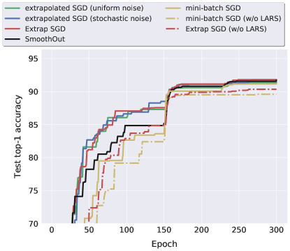
Figure 5: Understanding the learning behaviors of different methods on the large-batch training (with mini-batch size $8,192$ on $32$ workers) for training ResNet-20 on CIFAR-10. The hyper-parameters are fine-tuned, which are corresponding to the results shown in Table 1; by default the learning rate is decayed by $10$ at epoch $150$ and $225$.

The performance of post-local SGD, extrap-SGD and their combination on CIFAR10/100 is shown Table 2.

Table 2: The test top-1 accuracy of integrating extrap-SGD with post-local SGD (Lin et al., 2020). The performance of ResNet-20 on CIFAR-10/100 is evaluated with global mini-batch size $8,192$ ($K\!=\!32$). By default we use the learning rate scaling and warmup in Goyal et al. (2017) and LARS in You et al. (2017). We individually finetune $\gamma$ and $\tilde{\gamma}$ for each method; the local update step $H$ tuned from $\{4,8,16\}$ (as in Lin et al. (2020)) in general improves the performance and we report the best performance with $H\!=\!8$. The results are averaged over three different seeds.

	mini-batch SGD	mini-batch SGD (with post-local SGD)	extrap-SGD	extrap-SGD (with post-local SGD)
CIFAR-10	$91.36\pm 0.19$	$91.73\pm 0.25$	$91.72\pm 0.11$	$92.23\pm 0.02$
CIFAR-100	$65.79\pm 0.46$	$67.39\pm 0.18$	$66.63\pm 0.32$	$68.06\pm 0.21$

The effects of different combinations between local batch sizes and worker numbers are evaluated in Table 3.

Table 3: The test top-1 accuracy for ResNet-20 on CIFAR-10 under different combinations of local mini-batch size $B$ and number of workers $K$. The global mini-batch size is always set to $8,192$ and we vary $K$ workers (MPI processes). We individually finetune $\gamma$ and $\tilde{\gamma}$ for each method on different setups, and the reported results are averaged over three different seeds.

	$(B\!=\!512,K\!=\!16)$	$(B\!=\!256,K\!=\!32)$	$(B\!=\!128,K\!=\!64)$	$(B\!=\!64,K\!=\!128)$
Mini-batch SGD	$91.35\pm 0.19$	$91.36\pm 0.19$	$91.29\pm 0.13$	$91.32\pm 0.17$
extrap-SGD	$91.62\pm 0.32$	$91.72\pm 0.11$	$91.88\pm 0.27$	$91.89\pm 0.24$

E.2 LSTM on WikiText2

The learning curves of extrap-SGD and mini-batch SGD with LSTM model on WikiText2 dataset are presented in Figure 6.

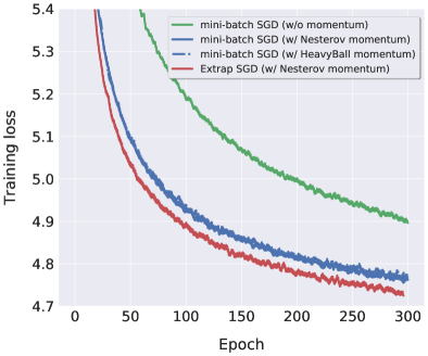
(a) $K\!=\!24$.

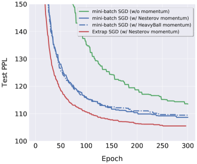
(b) $K\!=\!24$.

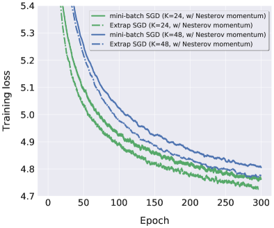
(c) $K\!=\!24$ V.S. $K\!=\!48$

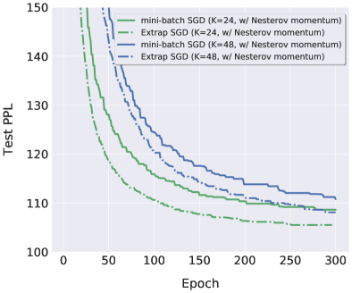
(d) $K\!=\!24$ V.S. $K\!=\!48$

Figure 6: The learning curves and perplexity (PPL, the lower the better) of training Wikitext-2 on LSTM. The global mini-batch size are $1536$ and $3072$ for $K\!=\!24$ and $K\!=\!48$ respectively, accounting for $2\%$ and $4\%$ of the total training data. We use the learning rate scaling and warmup in Goyal et al. (2017). We finetune the $\gamma$ for different variants of mini-batch SGD and extrap-SGD have no additional tuning. The results of the inline table are averaged over three different seeds.

E.3 Impact of different momentum factors

The impacts of momentum factors on extrap-SGD and mini-batch SGD are demonstrated in Figure 7 and Figure 8.

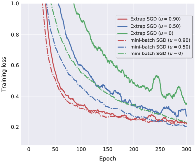
(a) The training loss of extrap-SGD v.s. Mini-batch SGD.

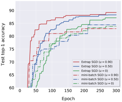
(b) The test top-1 accuracy of extrap-SGD v.s. Mini-batch SGD.

Figure 7: Understanding the behaviors of extrap-SGD and mini-batch SGD for different momentum factors $u$. The curves are evaluated on ResNet-20 with CIFAR-10 for mini-batch size $8,192$; we use constant learning rate $\gamma$ and the LARS trust term $\tilde{\gamma}$ over the whole training procedure, for both of mini-batch SGD and extrap-SGD (with default extrapolation term $\hat{\gamma}$). The value of $\gamma$ and $\tilde{\gamma}$ correspond to the tuned optimal value in Table 1.

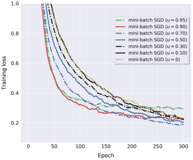
(a) The training loss of Mini-batch SGD.

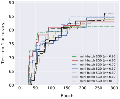
(b) The test top-1 accuracy of Mini-batch SGD.

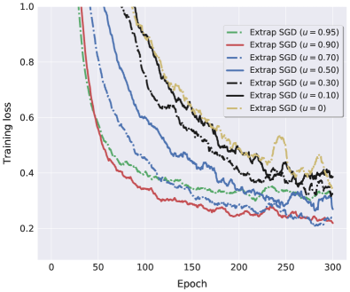
(c) The training loss of extrap-SGD.

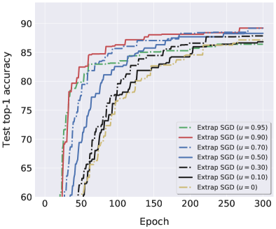
(d) The test top-1 accuracy of extrap-SGD.

Figure 8: The performance of extrap-SGD and mini-batch SGD for different momentum factors $u$. The curves are evaluated on ResNet-20 with CIFAR-10 for mini-batch size $8,192$; we use constant learning rate $\gamma$ and the LARS trust term $\tilde{\gamma}$ over the whole training procedure, for both of mini-batch SGD and extrap-SGD (with default extrapolation term $\hat{\gamma}$). The value of $\gamma$ and $\tilde{\gamma}$ correspond to the tuned optimal value in Table 1.

References

• Achille et al. (2019) Achille, A., Rovere, M., and Soatto, S. Critical learning periods in deep networks. In International Conference on Learning Representations, 2019. URL https://openreview.net/forum?id=BkeStsCcKQ.
• Chaudhari et al. (2017) Chaudhari, P., Choromanska, A., Soatto, S., LeCun, Y., Baldassi, C., Borgs, C., Chayes, J., Sagun, L., and Zecchina, R. Entropy-sgd: Biasing gradient descent into wide valleys. In International Conference on Learning Representations, 2017.
• Chavdarova et al. (2019) Chavdarova, T., Gidel, G., Fleuret, F., and Lacoste-Julien, S. Reducing noise in gan training with variance reduced extragradient. arXiv preprint arXiv:1904.08598, 2019.
• Daskalakis et al. (2017) Daskalakis, C., Ilyas, A., Syrgkanis, V., and Zeng, H. Training gans with optimism. arXiv preprint arXiv:1711.00141, 2017.
• Diakonikolas & Orecchia (2017) Diakonikolas, J. and Orecchia, L. Accelerated extra-gradient descent: A novel accelerated first-order method. arXiv preprint arXiv:1706.04680, 2017.
• Dinh et al. (2017) Dinh, L., Pascanu, R., Bengio, S., and Bengio, Y. Sharp minima can generalize for deep nets. arXiv preprint arXiv:1703.04933, 2017.
• Duchi et al. (2012) Duchi, J. C., Bartlett, P. L., and Wainwright, M. J. Randomized smoothing for stochastic optimization. SIAM Journal on Optimization, 22(2):674–701, 2012.
• Elliott et al. (2016) Elliott, D., Frank, S., Sima’an, K., and Specia, L. Multi30k: Multilingual english-german image descriptions. arXiv preprint arXiv:1605.00459, 2016.
• Garipov et al. (2018) Garipov, T., Izmailov, P., Podoprikhin, D., Vetrov, D. P., and Wilson, A. G. Loss surfaces, mode connectivity, and fast ensembling of dnns. arXiv preprint arXiv:1802.10026, 2018.
• Ghadimi & Lan (2016) Ghadimi, S. and Lan, G. Accelerated gradient methods for nonconvex nonlinear and stochastic programming. Mathematical Programming, 156(1-2):59–99, 2016.
• Gidel et al. (2018) Gidel, G., Berard, H., Vignoud, G., Vincent, P., and Lacoste-Julien, S. A variational inequality perspective on generative adversarial networks. arXiv preprint arXiv:1802.10551, 2018.
• Golatkar et al. (2019) Golatkar, A. S., Achille, A., and Soatto, S. Time matters in regularizing deep networks: Weight decay and data augmentation affect early learning dynamics, matter little near convergence. In Advances in Neural Information Processing Systems, pp. 10677–10687, 2019.
• Golmant et al. (2018) Golmant, N., Vemuri, N., Yao, Z., Feinberg, V., Gholami, A., Rothauge, K., Mahoney, M. W., and Gonzalez, J. On the computational inefficiency of large batch sizes for stochastic gradient descent. arXiv preprint arXiv:1811.12941, 2018.
• Goyal et al. (2017) Goyal, P., Dollár, P., Girshick, R., Noordhuis, P., Wesolowski, L., Kyrola, A., Tulloch, A., Jia, Y., and He, K. Accurate, large minibatch sgd: Training imagenet in 1 hour. arXiv preprint arXiv:1706.02677, 2017.
• Haruki et al. (2019) Haruki, K., Suzuki, T., Hamakawa, Y., Toda, T., Sakai, R., Ozawa, M., and Kimura, M. Gradient noise convolution (gnc): Smoothing loss function for distributed large-batch sgd, 2019.
• He et al. (2015) He, K., Zhang, X., Ren, S., and Sun, J. Delving deep into rectifiers: Surpassing human-level performance on imagenet classification. In Proceedings of the IEEE international conference on computer vision, pp.  1026–1034, 2015.
• He et al. (2016) He, K., Zhang, X., Ren, S., and Sun, J. Deep residual learning for image recognition. In Proceedings of the IEEE Conference on Computer Vision and Pattern Recognition, pp.  770–778, 2016.
• Hoffer et al. (2017) Hoffer, E., Hubara, I., and Soudry, D. Train longer, generalize better: closing the generalization gap in large batch training of neural networks. arXiv preprint arXiv:1705.08741, 2017.
• Huang et al. (2016a) Huang, G., Liu, Z., Weinberger, K. Q., and van der Maaten, L. Densely connected convolutional networks. arXiv preprint arXiv:1608.06993, 2016a.
• Huang et al. (2016b) Huang, G., Sun, Y., Liu, Z., Sedra, D., and Weinberger, K. Q. Deep networks with stochastic depth. In European Conference on Computer Vision, pp.  646–661. Springer, 2016b.
• Ioffe & Szegedy (2015) Ioffe, S. and Szegedy, C. Batch normalization: Accelerating deep network training by reducing internal covariate shift. arXiv preprint arXiv:1502.03167, 2015.
• Jastrzebski et al. (2020) Jastrzebski, S., Szymczak, M., Fort, S., Arpit, D., Tabor, J., Cho, K., and Geras, K. The break-even point on the optimization trajectories of deep neural networks. In International Conference on Learning Representations, 2020. URL https://openreview.net/forum?id=r1g87C4KwB.
• Juditsky et al. (2011) Juditsky, A., Nemirovski, A., and Tauvel, C. Solving variational inequalities with stochastic mirror-prox algorithm. Stochastic Systems, 1(1):17–58, 2011.
• Keskar et al. (2016) Keskar, N. S., Mudigere, D., Nocedal, J., Smelyanskiy, M., and Tang, P. T. P. On large-batch training for deep learning: Generalization gap and sharp minima. arXiv preprint arXiv:1609.04836, 2016.
• Kleinberg et al. (2018) Kleinberg, R., Li, Y., and Yuan, Y. An alternative view: When does sgd escape local minima?, 2018.
• Korpelevich (1976) Korpelevich, G. The extragradient method for finding saddle points and other problems. Matecon, 12:747–756, 1976.
• Krizhevsky & Hinton (2009) Krizhevsky, A. and Hinton, G. Learning multiple layers of features from tiny images. 2009.
• LeCun et al. (1991) LeCun, Y., Kanter, I., and Solla, S. A. Second order properties of error surfaces: Learning time and generalization. In Advances in neural information processing systems, pp. 918–924, 1991.
• Leng et al. (2017) Leng, C., Li, H., Zhu, S., and Jin, R. Extremely low bit neural network: Squeeze the last bit out with admm, 2017.
• Li et al. (2017) Li, H., Xu, Z., Taylor, G., and Goldstein, T. Visualizing the loss landscape of neural nets. arXiv preprint arXiv:1712.09913, 2017.
• Li et al. (2019) Li, Y., Wei, C., and Ma, T. Towards explaining the regularization effect of initial large learning rate in training neural networks. In Advances in Neural Information Processing Systems, pp. 11669–11680, 2019.
• Lin et al. (2020) Lin, T., Stich, S. U., Patel, K. K., and Jaggi, M. Don’t use large mini-batches, use local sgd. In International Conference on Learning Representations, 2020. URL https://openreview.net/forum?id=B1eyO1BFPr.
• Ma et al. (2017) Ma, S., Bassily, R., and Belkin, M. The power of interpolation: Understanding the effectiveness of sgd in modern over-parametrized learning. arXiv preprint arXiv:1712.06559, 2017.
• Masters & Luschi (2018) Masters, D. and Luschi, C. Revisiting small batch training for deep neural networks. arXiv preprint arXiv:1804.07612, 2018.
• McCandlish et al. (2018) McCandlish, S., Kaplan, J., Amodei, D., and Team, O. D. An empirical model of large-batch training. arXiv preprint arXiv:1812.06162, 2018.
• Merity et al. (2016) Merity, S., Xiong, C., Bradbury, J., and Socher, R. Pointer sentinel mixture models. arXiv preprint arXiv:1609.07843, 2016.
• Merity et al. (2017) Merity, S., Keskar, N. S., and Socher, R. Regularizing and optimizing lstm language models. arXiv preprint, pp.  arXiv:1708.02182, 2017.
• Mishchenko et al. (2019) Mishchenko, K., Kovalev, D., Shulgin, E., Richtárik, P., and Malitsky, Y. Revisiting stochastic extragradient. arXiv preprint arXiv:1905.11373, 2019.
• Nemirovski (2004) Nemirovski, A. Prox-method with rate of convergence o (1/t) for variational inequalities with lipschitz continuous monotone operators and smooth convex-concave saddle point problems. SIAM Journal on Optimization, 15(1):229–251, 2004.
• Nesterov (1983) Nesterov, Y. A method of solving a convex programming problem with convergence rate o (1/k2). In Soviet Mathematics Doklady, volume 27, pp.  372–376, 1983.
• Nesterov (2011) Nesterov, Y. Random gradient-free minimization of convex functions. CORE Discussion Papers 2011001, Université catholique de Louvain, Center for Operations Research and Econometrics (CORE), 2011. URL https://EconPapers.repec.org/RePEc:cor:louvco:2011001.
• Neyshabur (2017) Neyshabur, B. Implicit regularization in deep learning. arXiv preprint arXiv:1709.01953, 2017.
• Paszke et al. (2017) Paszke, A., Gross, S., Chintala, S., Chanan, G., Yang, E., DeVito, Z., Lin, Z., Desmaison, A., Antiga, L., and Lerer, A. Automatic differentiation in pytorch. In NIPS-W, 2017.
• Russakovsky et al. (2015) Russakovsky, O., Deng, J., Su, H., Krause, J., Satheesh, S., Ma, S., Huang, Z., Karpathy, A., Khosla, A., Bernstein, M., et al. Imagenet large scale visual recognition challenge. International Journal of Computer Vision, 115(3):211–252, 2015.
• Santurkar et al. (2018) Santurkar, S., Tsipras, D., Ilyas, A., and Madry, A. How does batch normalization help optimization? In Advances in Neural Information Processing Systems, pp. 2483–2493, 2018.
• Scaman et al. (2018) Scaman, K., Bach, F., Bubeck, S., Massoulié, L., and Lee, Y. T. Optimal algorithms for non-smooth distributed optimization in networks. In Advances in Neural Information Processing Systems, pp. 2740–2749, 2018.
• Shallue et al. (2018) Shallue, C. J., Lee, J., Antognini, J., Sohl-Dickstein, J., Frostig, R., and Dahl, G. E. Measuring the effects of data parallelism on neural network training, 2018.
• Simonyan & Zisserman (2014) Simonyan, K. and Zisserman, A. Very deep convolutional networks for large-scale image recognition. arXiv preprint arXiv:1409.1556, 2014.
• Stich & Karimireddy (2019) Stich, S. U. and Karimireddy, S. P. The error-feedback framework: Better rates for sgd with delayed gradients and compressed communication. arXiv preprint arXiv:1909.05350, 2019.
• Vaswani et al. (2017) Vaswani, A., Shazeer, N., Parmar, N., Uszkoreit, J., Jones, L., Gomez, A. N., Kaiser, Ł., and Polosukhin, I. Attention is all you need. In Advances in neural information processing systems, pp. 5998–6008, 2017.
• Wang & Srebro (2017) Wang, W. and Srebro, N. Stochastic nonconvex optimization with large minibatches. arXiv preprint arXiv:1709.08728, 2017.
• Wen et al. (2018) Wen, W., Wang, Y., Yan, F., Xu, C., Wu, C., Chen, Y., and Li, H. Smoothout: Smoothing out sharp minima to improve generalization in deep learning. arXiv preprint arXiv:1805.07898, 2018.
• Xu et al. (2019) Xu, Y., Yuan, Z., Yang, S., Jin, R., and Yang, T. On the convergence of (stochastic) gradient descent with extrapolation for non-convex minimization. Proceedings of the Twenty-Eighth International Joint Conference on Artificial Intelligence, Aug 2019. doi: 10.24963/ijcai.2019/556. URL http://dx.doi.org/10.24963/ijcai.2019/556.
• Yan et al. (2018) Yan, Y., Yang, T., Li, Z., Lin, Q., and Yang, Y. A unified analysis of stochastic momentum methods for deep learning. In IJCAI, pp.  2955–2961, 2018. URL https://doi.org/10.24963/ijcai.2018/410.
• Yao et al. (2018) Yao, Z., Gholami, A., Lei, Q., Keutzer, K., and Mahoney, M. W. Hessian-based analysis of large batch training and robustness to adversaries. arXiv preprint arXiv:1802.08241, 2018.
• Yin et al. (2017) Yin, D., Pananjady, A., Lam, M., Papailiopoulos, D., Ramchandran, K., and Bartlett, P. Gradient diversity: a key ingredient for scalable distributed learning. arXiv preprint arXiv:1706.05699, 2017.
• You et al. (2020a) You, K., Long, M., Wang, J., and Jordan, M. I. How does learning rate decay help modern neural networks? 2020a. URL https://openreview.net/forum?id=r1eOnh4YPB.
• You et al. (2017) You, Y., Gitman, I., and Ginsburg, B. Large batch training of convolutional networks. arXiv preprint arXiv:1708.03888, 2017.
• You et al. (2019) You, Y., Hseu, J., Ying, C., Demmel, J., Keutzer, K., and Hsieh, C.-J. Large-batch training for lstm and beyond. In Proceedings of the International Conference for High Performance Computing, Networking, Storage and Analysis, pp.  1–16, 2019.
• You et al. (2020b) You, Y., Li, J., Reddi, S., Hseu, J., Kumar, S., Bhojanapalli, S., Song, X., Demmel, J., Keutzer, K., and Hsieh, C.-J. Large batch optimization for deep learning: Training bert in 76 minutes. In International Conference on Learning Representations, 2020b. URL https://openreview.net/forum?id=Syx4wnEtvH.
• Yu et al. (2019) Yu, H., Jin, R., and Yang, S. On the linear speedup analysis of communication efficient momentum sgd for distributed non-convex optimization. arXiv preprint arXiv:1905.03817, 2019.
• Zhang et al. (2019) Zhang, J., Karimireddy, S. P., Veit, A., Kim, S., Reddi, S. J., Kumar, S., and Sra, S. Why adam beats sgd for attention models. arXiv preprint arXiv:1912.03194, 2019.