Spectral analysis, chiral disorder and topological edge states manifestation in open non-Hermitian Su-Schrieffer-Heeger chains

Abstract

We investigate topological and disorder effects in non-Hermitian systems with chiral symmetry. The system under consideration consists in a finite Su-Schrieffer-Heeger chain to which two semi-infinite leads are attached. The system lacks the parity-time and time-reversal symmetries and is appropriate for the study of quantum transport properties. The complex energy spectrum is analyzed in terms of the chain-lead coupling and chiral disorder strength, and shows substantial differences between chains with even and odd number of sites. The mid-gap edge states acquire a finite lifetime and are both of topological origin or generated by a strong coupling to the leads. The disorder induces coalescence of the topological eigenvalues, associated with exceptional points and vanishing of the eigenfunction rigidity. The electron transmission coefficient is approached in the Landauer formalism, and an analytical expression for the transmission in the range of topological states is obtained. Notably, the chiral disorder in this non-Hermitian system induces unitary conductance enhancement in the topological phase.

I Introduction

Different non-Hermitian models have been developed mainly for their exotic properties coming from the complex eigenvalues and biorthogonal eigenvectors, combined with different symmetry arguments. For instance, much attention has been paid to non-Hermitian models with parity-time ($\mathcal{PT}$) symmetry, which exhibit both real and complex eigenvalues depending on internal parameters Bender ; Bender1 . Such kind of non-Hermitian Hamiltonians are used for describing the gain and loss processes in optical lattices Nori ; Pan ; Poli ; Song .

There is a recent trend to identify topological phases in non-Hermitian systems. The question of defining bulk topological invariants and to find the correspondence to boundary states (the so-called bulk-boundary correspondence) is still a controversial discussion Yuce ; Kunst ; Yao ; Xiong ; Ueda ; Lee ; Leykam ; Takane ; Das ; Torres . In parallel, the disordered topological matter is also of considerable interest Jain ; Altland ; Prodan .

The Su-Schrieffer-Heeger (SSH) model is a platform commonly used for developing new topological concepts. Looking for new physics, the Hermitian model was extended by adding next-nearest-neighbor-hopping Platero , disorder Prodan , or expanding the unit cell Xie . In this paper, we look for the properties of the topological phase in open mesoscopic (finite-size) SSH systems. In this case, the non-Hermiticity is induced by the coupling to external reservoirs, and describes the electron transport problem. More explicitly, while the confined (finite) system is described by a Hermitian Hamiltonian, the open system obtained by attaching semi-infinite wires can be described by an effective Hamiltonian, which turns out to be non-Hermitian Rotter ; Moldoveanu ; ONA . As for the symmetries, the non-Hermitian Hamiltonian related to the open system lacks the time-reversal $\mathcal{T}$ and $\mathcal{PT}$ (its eigenvalues being always complex), but keeps the chiral symmetry $\mathcal{C}$ of the SSH chain.

In the present study, we demonstrate effects arising from non-Hermiticity and disorder, the purpose of the paper being twofold: i) to look for the fate of the mid-gap topological edge states when the coupling (hybridization) to the leads is introduced gradually, and ii) to study the competition between the coupling parameter (which controls the non-Hermiticity) and the disorder strength. We deliberately analyze the non-diagonal disorder (which affects the chain bonds) as it preserves the chiral symmetry of the SSH system and has the advantage of allowing an analytical solution.

Spectral and quantum transport quantities, describing the response of the topological states to the chain-lead coupling and chiral disorder, are calculated analytically and numerically. We deduce the exact analytical expression (22) of the electron transmission on the topological states, which shows a non-monotonic dependence on the coupling parameter and also a unitary peak. This behavior is explained in terms of density of states and is supported by the dwell time and the reflected flux delay.

The dependence of the transport properties on the disorder strength is nontrivial and allows for a disorder-induced conductance in the case of sufficiently strong coupling. The origin of this effect consists in the delocalization process of the edge states generated by the chiral disorder. It is to mention that the unitary transmission is conserved even in the disordered case.

We also find that, under the condition of strong hybridization, mid-gap edge states may occur even in the non-topological range of parameters. Another finding of interest is the level coalescence in the topological and non-topological phase, which can be induced by the chiral disorder, and depends on the chain length and the chain-lead coupling.

The paper is structured as follows: In Section II, we discuss the spectral properties of the topological phase for ordered and disordered finite SSH chains. The spectral properties of the non-Hermitian Hamiltonian in topological/non-topological phase, including the coalescence problem and the phase rigidity, are evidentiated in Section III. In Section IV, the quantum transport on the topological states (transmission coefficient, dwell time and reflected flux delay) is analyzed analytically and numerically. The section also highlights the chiral disorder effects on the density of states and transport properties. The results are summarized in the last section.

II Spectral properties of the finite SSH-chain with chiral disorder

The SSH model consists in a bipartite one-dimensional diatomic chain with alternating hopping parameters $t_{1}$ and $t_{2}$, which connect the sites of type $A$ and $B$. The model is described by the following tight-binding spinless Hermitian Hamiltonian:

$$H=t_{1}\sum_{i}c_{2i-1}^{{\dagger}}c_{2i}+t_{2}\sum_{i}c^{{\dagger}}_{2i}c_{2i+1}+H.c..$$ (1)

As we shall see, there are significant differences in the spectral and transport properties of the finite chains with even or odd number of sites. It is to remind that in the case of infinite chains, by imposing periodic boundary conditions, the Hamiltonian (1) can be rewritten in the momentum representation as:

$$\hskip 28.45274ptH=\sum_{\vec{k}}\left(\begin{array}[]{cc}a^{\dagger}_{k}{}&b^{\dagger}_{k}\end{array}\right)H(k)\left(\begin{array}[]{c}a_{k}\\ b_{k}\\ \end{array}\right),~{}~{}H(k)=(t_{1}+t_{2}cosk)\sigma_{x}+t_{2}sink\sigma_{y}.~{}~{}~{}~{}~{}~{}~{}~{}~{}~{}$$ (2)

where $\sigma_{x},\sigma_{y}$ are Pauli matrices. The above Hamiltonian shows chiral symmetry $\{\sigma_{z},H(k)\}=0$, but lacks both the parity $\mathcal{P}$ and time-reversal $\mathcal{T}$ symmetries. That is, the SSH model belongs to the AIII class Zirnbauer ; Ryu and may show a topological transition controlled by the ratio $t_{2}/t_{1}$ and specified by a winding number $\nu$.

In what concerns the finite chains, one may expect that the chain ends play a relevant role for the spectral and topological properties. Let us denote by $N_{A}$ and $N_{B}$, the number of A and B atoms in the finite chain, respectively. Assuming that the chain begins with A and ends also with A, the total number of lattice sites $N=N_{A}+N_{B}$ is odd, and $N_{A}-N_{B}=1$. Then, a theorem valid for bipartite lattices states that the energy spectrum contains at least one eigenvalue in the middle of the gap at $E=0$ Lieb ; Mielke . On the other hand, if the chain begins with A and ends with B, i.e., the total number of sites $N$ is even, one has $N_{A}-N_{B}=0$, and the minimum number of allowed states at the midgap equals zero.

In what concerns the topological properties, a guess can be done in advance. Since for N=odd the number of $t_{1}$-bonds and of $t_{2}$-bonds are equal, the ratio $t_{2}/t_{1}$ becomes meaningless as a criterion for a topological transition, so that we do not expect topological properties for SSH chains with an odd number of sites.

On the contrary, for N=even, as consequence of the bulk-edge correspondence, two topological edge states should appear if $t_{2}/t_{1}>1$, but they cannot be located strictly at zero energy, as this is forbidden by the before-mentioned theorem. The emergence of the topological states can be visualized by reducing gradually the hopping parameter $t_{N,1}$ between the last and the first site of the chain with periodic boundary condition. The decrease of $t_{N,1}$ breaks the periodicity and gives rise to a pair of states in the gap, which become quasi-degenerate in the middle of the gap as shown in Fig.1. The eigenvalues of several disordered configurations of the same chain are also shown in Fig.1 (blue points) in order to prove the robustness of the topological states created near $t_{1N}=0$ (in the domain encircled by the black curve).

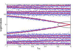
Figure 1: The crossover of the energy spectrum of the finite chain from periodic ($t_{1N}=1$) to open ($t_{1N}=0$) boundary condition. Eigenvalues of ten disordered configurations are superimposed over the spectrum of the ordered chain (shown in blue and red, respectively). The chain length is $N=40$, disorder strength is $W=0.7$, and $t_{2}/t_{1}=1.5$.

In what follows, we approach the question of the quantum states located in the middle of the gap in the case of finite SSH chains with an even number of sites, the only ones which are interesting from the topological point of view. Looking for the wave functions as:

$$|\Psi\rangle=\sum_{n=1}^{N_{c}}(\Psi^{A}_{n}a^{{\dagger}}_{n}|0\rangle+\Psi^{B}_{n}b^{{\dagger}}_{n}|0\rangle),$$ (3)

the following recurrence relations are obtained:

$$\hskip 71.13188ptt_{1}\Psi_{n}^{A}+t_{2}\Psi_{n+1}^{A}=E\Psi_{n}^{B}$$

$$\hskip 71.13188ptt_{1}\Psi_{n}^{B}+t_{2}\Psi_{n-1}^{B}=E\Psi_{n}^{A}.$$ (4)

As consequence of the inversion symmetry shown by the Hamiltonian in the case of even chains, one finds $|\Psi^{A}_{n}|=|\Psi^{B}_{N_{c}-n+1}|$. As the Hamiltonian anticommutes with the chiral operator

$$\mathcal{C}=\sum_{n=1}^{N_{c}}(a_{n}^{{\dagger}}a_{n}-b_{n}^{{\dagger}}b_{n}),$$ (5)

it is trivial to prove the electron-hole symmetry of the energy spectrum.

The question of finding the two quasi-degenerate energies in the middle of the spectrum will be approached perturbatively. In this spirit, let us accept for the beginning that $E=0$ is an eigenvalue and calculate the corresponding $\Psi^{A}_{n}and\Psi^{B}_{n}$. The recurrence relations (4) provide the following behavior of the coefficients:

$$\hskip 71.13188pt\Psi^{A}_{n}=(-t_{1}/t_{2})^{n-1}\Psi^{A}_{1}~{}~{}$$

$$\hskip 71.13188pt\Psi^{B}_{n}=(-t_{1}/t_{2})^{N_{c}-n}\Psi^{B}_{N_{c}}.$$ (6)

In the topological phase ($t_{2}/t_{1}>1$), $\Psi^{A}_{n}$ shows its maximum at $n=1$, while $\Psi^{B}_{n}$ reaches the maximum value at the other end of the chain $n=N_{c}$. It turns out that the functions $|\Psi^{A}>=\sum_{n}\Psi^{A}_{n}a^{{\dagger}}_{n}|0>$ and $|\Psi^{B}>=\sum_{n}\Psi^{B}_{n}b^{{\dagger}}_{n}|0>$ represent two orthogonal edge states, each one being localized at another end of the chain. The penetration length $\lambda$, defined as $|\Psi^{A}_{n}/\Psi^{A}_{1}|=exp\{-(n-1)/\lambda\}$, is given by:

$$\lambda^{-1}=\frac{1}{n-1}ln|\Psi^{A}_{n}/\Psi^{A}_{1}|=-ln(t_{1}/t_{2}),$$ (7)

and indicates that the strong localization of the edge states occurs for small ratios $t_{1}/t_{2}$. Obviously, the functions $\{|\Psi^{A}>,|\Psi^{B}>\}$ are only approximate eigenvectors of the finite chain Hamiltonian, corresponding to the approximate eigenvalue $E=0$. The actual eigenvectors can be written as their superposition, so that the secular equation gives the eigenvalues:

$$\hskip-3.98337ptE_{\pm}=\pm|<\Psi^{A}|H\Psi^{B}>|=\pm t_{2}(t_{1}/t_{2})^{N_{c}}|\Psi^{A*}_{1}\Psi^{B}_{N_{c}}|.$$ (8)

In conclusion, the above analytical calculation provides the splitting $\Delta=E_{+}-E_{-}$ between the energies of the two topological edge states and proves the exponential decay of the splitting in the limit of long chains.

In what follows we discuss the disorder effects on the penetration length $\lambda$ of the topological edge states is affected by disorder. we take into account the off-diagonal disorder obtained by considering the hopping parameter $t_{2}$ as a random variable, while $t_{1}$ is chosen as the energy unit ($t_{1}=1$). This is a chiral-type disorder in the sense that the Hamiltonian describing the disordered system preserves the anticommutation relation with the chiral operator $\mathcal{C}$ defined in (5), and, consequently, preserves the electron-hole spectral symmetry. To be specific, the hopping parameter $t_{2}$ is uniformly distributed in the range $[t_{2}-\frac{W}{2},t_{2}+\frac{W}{2}]$, where $W$ measures the disorder strength. Since the parameter $t_{2}$ becomes a random variable, Eq.(6) should be replaced by:

$$\Psi^{A}_{n}=\Pi_{i=1}^{n-1}(-t_{1}/t_{2}^{(i)})~{}\Psi^{A}_{1},$$ (9)

while the penetration length (7) should be redefined as the configurational average over all disorder realizations. Assuming a disorder strength $W<2t_{2}$ and $t_{1}=1$, one obtains:

$$\hskip-4.26773pt\frac{1}{\lambda}=\frac{-1}{n-1}<ln|\Psi^{A}_{n}/\Psi^{A}_{1}|>=\int_{-1/2}^{1/2}ln(t_{2}+Wx)dx,$$ (10)

which yields the following analytical expression:

$$\frac{1}{\lambda}=\frac{1}{W}[-W+(t_{2}+\frac{W}{2})ln(t_{2}+\frac{W}{2})-(t_{2}-\frac{W}{2})ln(t_{2}-\frac{W}{2})].$$ (11)

The dependence of $\lambda$ on the disorder strength $W$ is shown in Fig.2. One remarks the localization effect induced by the increase of $t_{2}$. However, more interesting is the delocalization process of the topological edge states expressed by the increasing penetration length $\lambda$, which takes place with increasing disorder. This result is in line with the finding in Prodan , where, for a generic one-dimensional (1D) disordered model, the topological phase ($\nu=1$) persists up to a given degree of disorder, where a localization-delocalization transition occurs.

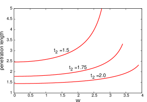
Figure 2: The penetration length $\lambda$ as function of the disorder strength $W$ for several values of the hopping parameter $t_{2}$. The increase of $\lambda$ indicates a delocalization process of the edge states.

III Spectral properties of the open SSH-chain: exceptional points and the rigidity of the wave function

The open system consists in a finite SSH chain to which two semi-infinite leads (probes) are attached at the sites n=1 and n=N, via the coupling parameter $\tau_{c}$ (see Fig.3). The leads are one-dimensional and described by an energy spectrum $E_{k}=2t_{L}cosk$. When coupled to leads, the SSH chain can be described by an effective Hamiltonian, which turns out to be non-Hermitian, with broken time-reversal symmetry:

$$H_{eff}=H+{\frac{\tau_{c}^{2}}{t_{L}}}e^{ik}(c_{1}^{{\dagger}}c_{1}+c^{{\dagger}}_{N}c_{N})$$ (12)

It is important to notice that $H_{eff}$ depends, via the parameter $k$, on the Fermi energy $E_{F}$ of the electrons in the leads. Throughout the paper, this energy will be chosen $E_{F}=0$, corresponding the $k=\pi/2$ in (12). At the same time, the hopping parameter $t_{1}$ present in $H$, is chosen as the energy unit ($t_{1}=1$), so that the problem is defined in the parameter space $\{t_{2},\tau_{c}\}$. As already discussed, the length $N$ of the SSH-chain is also an important quantity.

The deduction of Eq.(12) is rather simple and is based on a projection technique (see, for instance, the Green function approach in ONA ).

Figure 3: Schematic representation of the SSH chain, where A (red) and B(blue) represent the two atoms in the unit cell, $t_{1}$ connects the atoms in the same cell, and $t_{2}$ connects the atoms in adjacent cells. The first and the last site are connected to semi-infinite leads via the coupling parameter $\tau_{c}$, while $\tau_{l}$ is the hopping amplitude in the leads.

In order to obtain the complex eigenvalues of (12), one has to diagonalize the following matrix (written below for an even number of sites):

$${\bf H_{eff}}=\begin{pmatrix}i\tau_{c}^{2}/t_{L}&t_{1}&0&...&0\\ t_{1}&0&t_{2}&...&0\\ ...&...&...&...&...\\ 0&...&t_{2}&0&t_{1}\\ 0&...&0&t_{1}&i\tau_{c}^{2}/t_{L}\end{pmatrix}.$$ (13)

Before discussing the complex spectrum of longer chains, it is helpful to analyze two short chains, with N=3 and N=4, which allow analytical solutions. These examples make clear the spectral differences between the even and odd chains, mainly in the context of the so-called exceptional points. For $N=3$, the three eigenvalues read:

$$\omega_{0}=i\tau^{2}_{c}/t_{L},~{}~{}~{}~{}~{}~{}~{}~{}~{}~{}~{}~{}~{}~{}~{}~{}~{}~{}~{}~{}~{}~{}~{}~{}~{}~{}~{}~{}~{}~{}~{}~{}~{}~{}~{}~{}~{}~{}~{}~{}~{}$$

$$\omega_{\pm}=\frac{1}{2}\big{(}i\tau^{2}_{c}/t_{L}\pm\sqrt{(i\tau^{2}_{c}/t_{L})^{2}+4(t_{1}^{2}+t_{2}^{2})}~{}\big{)}.$$ (14)

For $N=4$, the four eigenvalues read:

$$\omega_{1,\pm}=\frac{1}{2}\big{(}i\tau^{2}_{c}/t_{L}+t_{2}\pm\sqrt{(i\tau^{2}_{c}/t_{L}+t_{2})^{2}+4t_{1}^{2})}~{}\big{)},$$

$$\omega_{2,\pm}=\frac{1}{2}\big{(}i\tau^{2}_{c}/t_{L}-t_{2}\pm\sqrt{(i\tau^{2}_{c}/t_{L}-t_{2})^{2}+4t_{1}^{2})}~{}\big{)}.$$ (15)

An exceptional point (EP) is defined by the degeneracy of two eigenvalues of the non-Hermitian Hamiltonian, which comes out at a given value of the coupling $\tau_{c}$. At such a point, one occurs the coalescence at $ReE=0$ of the real parts of the two eigenvalues and also the bifurcation of the imaginary parts.

One notices from Eq.(14) that, in the odd case N=3, the condition $\omega_{+}=\omega_{-}$ is fulfilled when the quantity under the radical vanishes, i.e. at $\tau_{c}^{2}=2t_{L}\sqrt{t_{1}^{2}+t_{2}^{2}}$. One observes also that the imaginary part of the energies $\omega_{\pm}$ is a nonanalytical function of $\tau_{c}$, as all derivatives diverge at EP.

On the contrary, in the case N=4 described by Eq.(15), the necessary condition for an EP, which in this case reads as $\omega_{1-}=\omega_{2+}$, cannot be fulfilled (except for $t_{2}=0$, meaning in fact a broken chain).

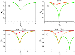
Figure 4: Phase rigidity in the non-topological case ($t_{2}/t_{1}=0.5$) for ordered/disordered chains with even/odd number of sites as function of the coupling strength. Panels a) and c) show that for ordered even chains of length $N=4,6$ the EP is missing, however it appears for the ordered odd chain with $N=5$ (panel b). The significant result is that the chiral disorder induces EP in an even chain, too (see the green line in panel d).

The question of exceptional points can be discussed also in terms of eigenfunction phase rigidity, defined as:

$$r_{i}=\frac{|<\Psi_{i}^{L}|\Psi_{i}^{R}>|}{<\Psi_{i}^{R}|\Psi_{i}^{R}>},$$ (16)

where $<\Psi_{i}^{L}|$ and $|\Psi_{i}^{R}>$ are the left and right biorthogonal eigenvectors of the non-Hermitian Hamiltonian, and $i$ is the eigenvector index. The rigidity measures the degree of biortogonality of the eigenfunctions and depends on the strength of the coupling with the infinite leads. Obviously, for the Hermitian case $\tau_{c}=0$ one has $<\Psi_{i}^{L}|=<\Psi_{i}^{R}|$ such that $r_{i}=1$. With increasing $\tau_{c}$ the rigidity decreases, and one proves Rotter that the coalescenting states show $r=0$ at the EP. This is the case in Fig.4b for an ordered chain of length $N=5$. As a counterexample, Fig.4a and Fig.4c show a non-vanishing phase rigidity for chains with an even number of sites ($N=4$ and $N=6$, respectively) and under non-topological condition $t_{2}/t_{1}<1$. Nevertheless, the presence of rigidity dips in these figures indicates a quasi-degeneracy of the real parts, and a smooth branching of the imaginary parts of the involved eigenvalues. One may suspect that in the limit of $N\rightarrow\infty$ the rigidity $r_{i}\rightarrow 0$.

The analytical formulas for N=3 and N=4 and also the numerical results for longer chains suggest that EPs are exhibited only by SSH chains with an odd number of sites. The distinction between the odd and even chains consists in the absence, and respectively, the presence of the spatial inversion symmetry. Apparently, the presence of this symmetry prevents the appearance of exceptional points in the open SSH chains with even number of sites. We have not a proof of that, nevertheless the study of disordered chains gives support to this argument. Indeed, the chiral disorder introduced into chains with N=even breaks the previous inversion symmetry, and, at the same time, gives rise to a vanishing phase rigidity. This result is obvious by comparing Fig.4c and Fig.4d.

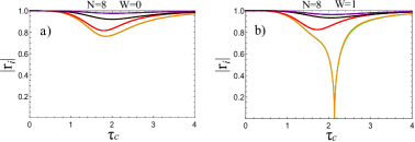
Figure 5: Phase rigidity in the topological case ($t_{2}/t_{1}=1.5$) as function of the coupling strength. The states showing the vanishing rigidity in the presence of disorder ($W=1$) are the topological ones.

The eigenfunction phase rigidity induced by the non-Hermitian perturbation occurs also in the topological phase ($t_{2}/t_{1}>1$), as shown in Fig.5. The vanishing rigidity is due again to the chiral disorder, and it is exhibited by the topological eigenstates.

The way the parameter $\tau_{c}$ controls this effect can be followed by looking at the flow of the eigenvalues in the complex plane {Im E, Re E} when $\tau_{c}$ is varied (see Fig.6). At $\tau_{c}=0$, the eigenvalues are real and the splitting between the two topological levels is that one given by Eq.(8). An analytic perturbative approach shows readily that for small $\tau_{c}$ the real parts of the topological eigenvalues attract each other. By numerical calculation, one finds that also for larger coupling the real parts keep getting closer, while the imaginary part increases. Finally, there is a value of $\tau_{c}$ where the real parts of the two eigenvalues coalesce at $ReE=0$, while the imaginary parts continue to increase.

Strictly specking, only the disordered chain (blue curve in Fig.6) shows a rigorous coalescence, which corroborates the exceptional point shown by the phase rigidity in Fig.5b. In what concerns the ordered chain (red curve in Fig.6), the coalescence is only approximate, in agreement with the above discussion.

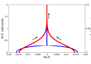
Figure 6: The flow in the complex plain of the eigenvalues corresponding to the two topological edge states, when the chain-lead coupling $\tau_{c}$ is increased continuously. The ordered chain is described by the red curve, while a disordered chain with $W=1$ is described by the blue one. The arrows indicate the increasing $\tau_{c}$. (other parameters: $t_{2}/t_{1}=1.5,N=20$).

Taking into account that for the infinite SSH chain the ratio $t_{2}/t_{1}$ dictates the presence of the topological phase, it becomes of interest to study the role of this parameter also in the case of open finite chains. In what follows, we illustrate how the external leads affects the midgap edge modes already developed in the confined finite chain (and discussed in Section II). We also detect a new type of midgap edge states in the non-topological range ($t_{2}/t_{1}<1$), which are generated by the strong coupling to the leads.

The real and imaginary part of the energy spectrum of the open SSH chain of length N=20 is shown in Fig.7 as function of the parameter $t_{2}/t_{1}$, for different values of the chain-lead coupling $\tau_{c}$. The weak coupling case ($\tau_{c}=0.1$) shows in Fig.7a that the real part of two states detach themselves gradually from bands with increasing ratio $t_{2}/t_{1}$ and merge continuously into two quasi-degenerate midgap edge states. At the same time, the eigenvalues acquire a large imaginary part shown in Fig.7b, which denotes a short lifetime (defined as $\tau=\hbar/ImE$) of the topological edge states in the presence of the leads. This behavior of the complex spectrum at weak coupling is equivalent to the transition from the insulating to topological phase for an infinite chain (without leads), which however occurs sharply at $t_{2}/t_{1}=1$.

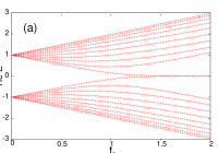
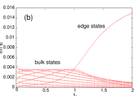
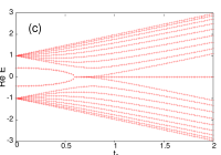
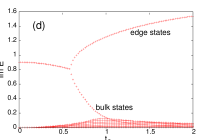
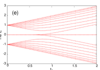
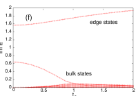
Figure 7: Real and imaginary parts of the eigenvalues of the effective Hamiltonian (12) as function of the hopping amplitude $t_{2}$, for an open chain with $N=20$, at different chain-lead couplings: $\tau_{c}=0.1$ (panels (a) and (b)), $\tau_{c}=1.9$ (panels (c) and (d)), $\tau_{c}=2.1$ (panels (e) and (f)). The imaginary part indicates that the edges states have a much shorter lifetime $\tau=\hbar/ImE$ than the bulk states.

An increased coupling reveals new physics as illustrated in Fig.7c and Fig.7d. This time, two levels detach themselves from each band at small $t_{2}$, next they become quasi-degenerate at $ReE=0$, and, finally, they split at large $t_{2}$ into two states that return to the bands, and the two topological mid-gap edge states. This level separation exhibited by the real part of the spectrum is accompanied by a branching of the corresponding imaginary parts, which show large values (i.e., small lifetime) for the edge modes, but a decreasing imaginary energy (i.e., increasing lifetime) of the states returning to the bands.

Fig.7e and Fig.7f describe the case of an even stronger coupling ($\tau_{c}=2.1$). This time, four mid-gap edge states are generated, which, with increasing $t_{2}$, evolve again into two longlife band states and two topological edge states with a small lifetime. The hint for understanding why there are four edge states at small $t_{2}$ and strong $\tau_{c}$ comes from the formation of A-B dimers at each end of the chain, which sum up a total number of four quantum states. Strictly at $t_{2}=0$, the eigenvalues corresponding to such a dimer can be obtained immediately as:

$$E=\frac{1}{2}\big{(}\frac{i\tau_{c}^{2}}{t_{L}}\pm\sqrt{-\frac{\tau_{c}^{4}}{t_{L}^{2}}+4t_{1}^{2}}~{}\big{)},$$ (17)

and it is obvious that for sufficiently big $\tau_{c}$, the eigenvalues are purely imaginary, i.e., the states become of midgap-type.

The above examination of the spectral properties emphasizes that the coupling to the leads assigns a finite lifetime to the topological edge states, which is much shorter than that one of the bulk states. Moreover, one can show numerically that the degree of localization near the chain ends increases with increasing chain-lead coupling. Secondly, we find that the coupling is able to generate edge states in the gap even under non-topological conditions (i.e., for $t_{2}/t_{1}<1$) if the parameter $\tau_{c}$ is sufficiently strong.

IV Quantum transport on topological edge states and chiral disorder effects

From the point of view of the charge transport through the SSH chain, one may expect, at the first sight, that the conductance should vanish in the range of the topological states because of their localized character. However, the numerical calculation based on the Landauer approach indicates a non-vanishing transmission coefficient at energies in the middle of the gap, where the topological states are located (see Fig.8). An exact analytical calculation is also accessible for the energy $E=0$, and the result Eq.(22) indicates the same, and also the vanishing of the conductance in the limit of long chains.

Obviously, the coupling to external leads should affect mostly the conductance of the states localized at the edges of the system, and this is indeed visible in Fig.8. One notices that for small coupling $\tau_{c}$ the two peaks in the middle of the spectrum are well separated, but with increasing $\tau_{c}$ they overlap and ends up with a fast decay of the transmission.

With the effective Hamiltonian (16) at hand, one may calculate the Green function $G(z)=(z-H_{eff})^{-1}$ that enters the expression of the transmission coefficient in the Landauer-Büttiker formalism. The Fermi energy in the leads being fixed at $E_{F}=0$, the whole energy spectrum of the SSH chain can be scanned by applying a gate potential $V_{gate}$, which is varied continuously Note-Vg . Assuming that the leads are attached to the first and last site $n=1,N$ of the SSH chain, the transmission coefficient is given in units $e^{2}/h$ by Caroli :

$$T(V_{gate},\tau_{c})=\frac{4\tau_{c}^{4}}{t_{L}^{2}}|G_{1N}(V_{g})|^{2}sin^{2}k=\frac{4\tau_{c}^{4}}{t_{L}^{2}}|<1|(V_{g}-H_{eff})^{-1}|N>|^{2}sin^{2}k,$$ (18)

where $sink$ comes from the density of states in the semi-infinite leads. We remind that $E_{F}=0$ corresponds to $sink=1$.

Usually, Eq.(18) is evaluated numerically by scanning the whole spectrum as it is shown in Fig.8 for a chain of length $N=8$. One remarks that the transmission peaks on the bulk states show a robust unitary limit ($T=1$) with respect to lead-chain coupling strength, while the transmission on the topological states is very sensitive to this coupling.

It is notable that $T(V_{gate}=0)$, which corresponds to the electron transmission at the middle of the gap, can be calculated analytically exact.

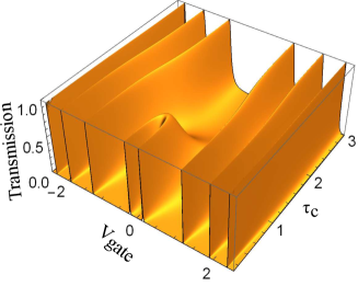
Figure 8: Transmission coefficient as function of the chain-lead coupling $\tau_{c}$ for the SSH chain of length $N=8$. The lateral peaks correspond to the six bulk states, the central peaks are due to the topological edge states ($t_{1}=1,t_{2}=1.5$).

To this aim, besides the function $G$, one has to consider $G^{0}(z)=(z-H)^{-1}$, of the finite (isolated) SSH chain. Then, the matrix element $G_{1N}$, needed in Eq.(18), is given by the Dyson equations:

$$\hskip 56.9055ptG_{1N}=G^{0}_{1N}+G^{0}_{11}\gamma G_{1N}+G^{0}_{1N}\gamma G_{NN},~{}~{}~{}~{}$$

$$\hskip 56.9055ptG_{NN}=G^{0}_{NN}+G^{0}_{N1}\gamma G_{1N}+G^{0}_{NN}\gamma G_{NN},$$ (19)

with $\gamma=i(\tau_{c}^{2}/t_{L})$ (see Eq.12). It results immediately:

$$G_{1N}=G^{0}_{1N}/[(1-\gamma G^{0}_{11})(1-\gamma G^{0}_{NN})-\gamma^{2}G^{0}_{1N}G^{0}_{N1}].$$ (20)

The matrix elements of $G^{0}$ can easily be calculated analytically using the recipe Fonseca for the inversion of tridiagonal matrices:

$$G^{0}_{1N}=\big{(}H^{-1}\big{)}_{1N}={\frac{1}{t_{2}}}\big{(}\frac{t_{2}}{t_{1}}\big{)}^{N/2},$$ (21)

and also $G^{0}_{11}=G^{0}_{NN}=0$. By using these expressions in (20), and next in (18), we obtain the following analytical formula for the transmission coefficient of the SSH finite ordered chain with an even number of sites:

$$T(V_{gate}=0,\tau_{c})=\frac{\big{(}4\tau_{c}^{4}/{t_{L}}^{2}t_{2}^{2}\big{)}(t_{2}/t_{1})^{N}}{[1+\big{(}\tau_{c}^{4}/{t_{L}}^{2}t_{2}^{2}\big{)}(t_{2}/t_{1})^{N}]^{2}}.$$ (22)

The transmission coefficient (22) shows an intriguing non-monotonous dependence on the chain-lead coupling parameter $\tau_{c}$, which is depicted in Fig.9a (red curve). The maximum corresponds to a unitary transmission, the position of which can be deduced immediately as:

$$\tau_{c}^{max}=\sqrt{t_{L}t_{2}}\big{(}t_{1}/t_{2}\big{)}^{N/4}.$$ (23)

One observes in Fig.9a that the disorder gives rise to a shift to the right of this maximum. This aspect cannot be overlooked as it proves a disorder induced increase of the transmission coefficient, whenever the chain-lead coupling is strong enough.

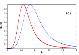
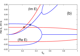
Figure 9: Transmission coefficient at $E=0$ (a) and complex topological eigenvalues (b) as function of the chain-lead coupling $\tau_{c}$ for ordered (red) and disordered (blue) SSH chain. In both cases, the unitary peak of $T(E)$ corresponds to the intersection $ReE=ImE$ in the spectrum ($N=20,t_{2}/t_{1}=1.5,W=2$).

Aiming to get insight into the physics behind the non-monotonous behavior of the transmission coefficient, we approach below the question of the density of states DoS in the energy range of the topological states. Obviously, the coupling to the leads gives rise to the broadening of the energy levels. The resulting overlap of the energy tails creates a non-vanishing (and increasing with $\tau_{c}$) density of states at $E=0$, which can support the increase of the transmission coefficient on the left-hand side of the red curve in Fig.9a. On the other hand, one may also speculate that the coalescence process shown in Fig.6 affects the DoS at high values of the coupling parameter.

Formally, the density of states reads:

$$\begin{split}g(E,\tau_{c})&=-\frac{1}{\pi}Im\sum_{i}\langle\Psi_{i}|(E-H_{eff})^{-1}|\Psi_{i}\rangle\\ &=-\frac{1}{\pi}Im\sum_{i}(E-ReE_{i}+iImE_{i})^{-1},\end{split}$$ (24)

however at $E=0$, only the two poles coming from the topological levels $E_{-}$ and $E_{+}$ contribute to the density of states. Since the real parts of two levels are symmetric about $ReE=0$ ($ReE_{+}=-ReE_{-}=\Delta/2$), and the imaginary parts are the same ($ImE_{-}=ImE_{+}=\Gamma$), one obtains:

$$g(E=0,\tau_{c})=\frac{2}{\pi}\frac{\Gamma(\tau_{c})}{\Delta^{2}(\tau_{c})/4+\Gamma^{2}(\tau_{c})}.$$ (25)

Let us calculate the real and imaginary part of $E_{+}$ and $E_{-}$ and represent them simultaneously in Fig.9b. We note that $|ReE_{\pm}|$ decreases with $\tau_{c}$, while the imaginary part behaves oppositely. As a result, as long as $\Delta/2>\Gamma$, the density of states (25) increases with $\tau_{c}$, but decreases in the opposite case $\Delta/2<\Gamma$. So, the maximum of the density of states is reached for that value of $\tau_{c}$ where the real and imaginary part of the topological eigenvalues intersect:

$$\Delta(\tau_{c})/2=\Gamma(\tau_{c}).$$ (26)

The first remark is that the value of $\tau_{c}$ corresponding to the intersection coincides with the value of $\tau_{c}$ where the transmission coefficient reaches its maximum in Fig.9a. This occurs both for the ordered and disordered chain (red and blue curves, respectively). The second remark is that the curves corresponding to the disordered chain, intersect at a higher value of the coupling than for the ordered chain. The implications of this last observation will be discussed later in the context of disorder effects.

According to Fig.6, for larger couplings, close to the coalescence, one has $\Delta(\tau_{c})\approx 0$, while $\Gamma(\tau_{c})$ keeps increasing with $\tau_{c}$, fact that implies a small lifetime $\tau=\hbar/\Gamma$ of the topological states. In this range, the density of states (25) becomes:

$$g(E=0,\tau_{c})=2/\pi\Gamma=2\tau/\pi\hbar.$$ (27)

It turns out that the continuous decrease of the lifetime gives rise to the continuous depletion of the density of states, which in turn yields the decrease of the transmission coefficient also beyond the coalescence point.

The conclusion of the above discussion is that the non-monotonous behavior of $T(V_{gate}=0,\tau_{c})$ follows the behavior of the density of states in the middle of the gap.

As we have already discussed, the non-Hermitian Hamiltonian (12), which describes the transport problem, does not exhibit exceptional points in the case of ordered even chains. However, let us consider also an associated Hamiltonian:

$$H_{PT}=H+\frac{i\tau_{c}^{2}}{t_{L}}(c_{1}^{{\dagger}}c_{1}-c_{N}^{{\dagger}}c_{N}),$$ (28)

which shows $\mathcal{PT}$-symmetry and an exceptional point, which depends on $\tau_{c}$. It is remarkably interesting that the position of the EP shown by the spectrum of (28) coincides with the transmission peak position at $\tau_{c}=\tau_{c}^{max}$. This can easily be proved analytically (by looking for the poles of the Green function $G(z)=(z-H_{PT})^{-1}$) and checked numerically by calculating the energy spectrum. Such spectral similarities between the two Hamiltonians of the ordered chains are studied also in Gorbatsevich .

More insight on the manifestation of the topological states in open systems can be obtained by examining other relevant quantities, like the dwell time and reflected flux delay.

The dwell time $\tau_{D}$ measures the time spent in the system by the electron injected from the lead. According to the definition Buettiker , the calculation of the dwell time pretends the knowledge of the probability to find the incident particle inside the barrier, which next has to be divided by the incident current. For our specific problem, the barrier consists of the SSH chain, and the quantities of interest are to be calculated in the energy range of the topological states.

The Lipmann-Schwinger formalism provides the scattering wave function $|\Psi^{scatt}\rangle$, which we project on all sites $n$ of the chain. Then, the probability to find the particle inside the chain is $\sum_{n}|\langle n|\Psi^{scatt}\rangle|^{2}$, and is given by the following expression, which we use to calculate $\tau_{D}$ numerically:

$$\sum_{n}|\langle n|\Psi^{scatt}\rangle|^{2}=\tau_{c}^{2}\sum_{n}|\langle n|H_{eff}^{-1}|1\rangle|^{2}.$$ (29)

(Notice that the above formula assumes the electron to be injected at the site $n=1$. The technicalities related to the deduction of (29) can be found in ONA , and are no more repeated here.)

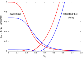
Figure 10: Dwell time and inverse of the reflected flux delay as function of the coupling parameter $\tau_{c}$ for ordered (red curves) and disordered (blue curves) SSH chain in the topological phase ($t_{2}/t_{1}=1.5,N=20,W=2$). The dwell time is scaled to have the maximum at $\tau_{D}=1$.

In contrast to the transmission coefficient, the dwell time plotted in Fig.10 exhibits a monotonous decrease with the coupling parameter, with a significant drop about $\tau_{c}=\tau_{c}^{max}$. One knows Winful that $\tau_{D}$ cannot distinguish between the transmitted and reflected flux, such that one cannot say a priori whether the decay comes from an increasing transmission or increasing reflection.

In the range of low coupling, the answer to the above question is simple, as the increasing transmission (observable in Fig.9a for $\tau_{c}<\tau_{c}^{max}$) obviously contributes to reducing the time $\tau_{D}$ spent by the charge inside the system. On the other hand, for strong coupling, we know (again from Fig.9a) that the transmission falls down drastically, such that the prevailing process in this range should be the reflection.

The above conclusion is reinforced by the behavior of the reflected flux delay defined as $\tau_{R}=\tau_{D}/(1-T^{2})$. It is to remind that a small $\tau_{R}$ evidentiates a strong reflection process. Then, by observing the behavior of $1/\tau_{R}$ in Fig.10, one notices indeed a strong reflection in the range of large coupling $\tau_{c}$. One may also observe that the zero of the reflected flux delay coincides with the unitary maximum of the transmission coefficient in Fig.9a.

In what follows, we examine the combined effect of the chiral disorder and chain-lead coupling on the transport properties of the SSH chain. Using (18), the transmission coefficient can be calculated for any given disorder configuration. Fig.9a exhibits the transmission coefficient as function of the coupling for both the ordered chain (red curve) and a disordered chain with $W=2$ (blue curve).

The comparison of the two curves highlights a surprising behavior, namely: for weak coupling (small $\tau_{c}$), the disorder effect consists in reducing the transmission, however, in the range of strong coupling, the effect is opposite. One notices that the significantly different behaviors are associated to the shift with disorder of the transmission peak. The shift infers that the condition (26), telling where the maximum occurs, is satisfied at higher values of $\tau_{c}$ in the disordered case. This is indeed numerically confirmed in Fig.9b by the intersection of the blue curves, which describe the real and imaginary part of the topological eigenvalues in the disordered case. The shift of the transmission peak can be understood by replacing the hopping parameter $t_{2}$ in the expression (23) for $\tau_{c}^{max}$ with a smaller effective $t_{2}^{eff}$ acting in the disordered case. We estimate below this effective parameter in the case of weak disorder.

Let us remind that the chiral disorder is introduced by turning $t_{2}$ in each cell of the ordered chain (indexed by $i=1,...,N_{c}$) into a random variable $\{t_{2}^{(i)}\}$, which is equally distributed in the range $[-\frac{W}{2},\frac{W}{2}]$. A constraint on the mean value is imposed for each disorder configuration, namely: $\frac{1}{N_{c}}\sum_{i}t_{2}^{(i)}=t_{2}$. With $t_{2}^{(i)}=t_{2}+\delta_{i}$, the constraint becomes $\sum_{i}\delta_{i}=0$. Then, any quantity of the type $t_{2}^{N_{c}}$, which appears in formulas describing the ordered chain (as, for instance, in (21)), should be replaced by the configurational average $<\Pi_{i=1}^{N_{c}}t_{2}^{(i)}>$. For weak disorder, keeping only the terms up to the second power in $\delta$, one obtains:

$$<\Pi_{i=1}^{N_{c}}t_{2}^{(i)}>\approx t_{2}^{N_{c}}+t_{2}^{N_{c}-2}\sum_{i}\sum_{j<i}<\delta_{i}\delta_{j}>.$$ (30)

The fluctuations $<\delta_{i}\delta_{j}>$ are easily estimated from:

$$<\big{(}\sum_{i}\delta_{i}\big{)}^{2}>=\sum_{i}<\delta_{i}^{2}>+2\sum_{i}\sum_{j<i}<\delta_{i}\delta_{j}>=0,$$ (31)

where, for the specific disorder distribution, the variance is known to be $<\delta_{i}^{2}>=\frac{W^{2}}{12}$. It results that, for weak disorder,

$$<\Pi_{i=1}^{N_{c}}t_{2}^{(i)}>=t_{2}^{N_{c}}\big{(}1-\frac{N_{c}}{24}\frac{W^{2}}{t_{2}^{2}}\big{)},$$ (32)

proving that the disorder induced effective hopping parameter $t_{2}^{eff}$ is smaller than $t_{2}$:

$$t_{2}^{eff}=t_{2}\sqrt[N_{c}]{1-\frac{N_{c}}{24}\frac{W^{2}}{t_{2}^{2}}}.$$ (33)

This result is responsible for the shift of the transmittance peak in Fig.9a, but also for the disordered increased splitting $E_{+}-E_{-}$, which can be noticed in Fig.9b. Obviously, the longer the chain, the smaller the disorder for which (33) is valid.

A full description, for any disorder, of the transmission on the topological states in the parameter space $\{W,\tau_{c}\}$ is given in Fig.11. The two cases shown in Fig.9a for $W=0,2$ can be identified immediately. The figure brings into attention the position of the transmission peak (red region), which evolves versus higher values of the coupling as the disorder is increased. This occurs, however, only up to $W\approx 3$. Above this value, the topological states are mixed up with disordered states coming from the bands, so that the topological phase is destroyed.

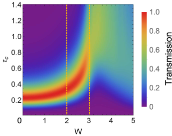
Figure 11: Transmission coefficient at $V_{gate}=0$ in the topological phase $t_{2}/t_{1}=1.5$ as a function of the disorder strength $W$ and coupling parameter $\tau_{c}$, calculated by averaging over 1000 disorder configurations. The dashed line at $W=2$ corresponds to the disordered case in Fig.9a. The dashed line at $W=3$ represents the border above which the bulk states coming from the two bands mix up with the topological states. The number of sites is $N=20$.

For fixed values of the lead-chain coupling, different regimes can be observed in Fig.11. At very small and large values of $\tau_{c}$ the transmission coefficient vanishes. However, two types of disorder dependence can be detected in the range of interest about the transmission peak. As examples, we observe that at $\tau_{c}=0.2$, the transmission decreases with the disorder strength $W$, however, at $\tau_{c}=0.4$ the transmission is enhanced in the presence of disorder. The enhancement occurs only for sufficiently large $\tau_{c}$, the effect being apparent in Fig.11 for $\tau_{c}\gtrsim 0.3$.

To understand the above effect, one has to keep in mind that, being localized near the ends of the chain, the topological states conduct only inasmuch as they penetrate the middle of the chain. Hence, the disorder-driven increase of the transmission should be accompanied by a corresponding change in the local density of states along the chain. The expectation is confirmed by the numerical calculation of the LDoS:

$$g_{n}(E=0)=-(1/\pi)Im\langle n|H_{eff}^{-1}n\rangle.$$ (34)

Indeed, in Fig.12 we observe that the local density of states in the middle of the chain is sensible higher in the disordered case (green and blue curves) than in the ordered one (red curve).

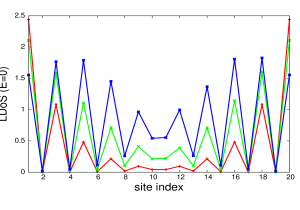
Figure 12: Local density of states at $E=0$ in the ordered and disordered case, corresponding to $W=0$ (red), $W=2$ (green) and $W=2.5$ (blue). Note that the disorder increases the density of states in the middle of the chain. In the disordered case, one averages over 5000 configurations ($t_{2}/t_{1}=1.5,\tau_{c}=0.5$).

The response to the chiral disorder shown by the open SSH chain in the case of strong coupling represents a signature of the disorder-driven electron conductance in 1D systems. This effect was already met in two-dimensional systems (2D) like topological Anderson insulators (TAI) Jain , or in the situation when the edge states coexist with bulk states and become functionalized by disorder Baum ; Bogdan . The possibility of finding the TAI phase in disordered wires, and also in disordered gain-loss 1D systems is discussed in Meier ; Luo .

We conclude the chapter by investigating the disorder effect on the dwell time and reflected flux delay, the result being shown in Fig.10 (blue curves). The first notable effect is the reduced value of $\tau_{D}$ in comparison with the ordered case, visible in the range of low coupling. As the transmission is also reduced in this range, the small dwell time comes from the disorder increased reflectivity.

In what concerns the reflected flux delay, the range of interest is $\tau_{c}>\tau_{c}^{max}$, where the smaller values of $1/\tau_{R}$ (compared to the ordered case) mean a lower reflectivity and, automatically, a higher transmission caused by disorder.

It turns out that the response to disorder of the local density of states, dwell time and reflected flux delay endorse the behavior of the transmission coefficient in the presence of the chiral disorder for the entire range of the lead-chain coupling.

V Summary and conclusions

The paper has two main objectives: to observe the fate of the topological edge states, pre-existing in the finite SSH chain, when the system is opened by attaching semi-infinite leads, and to find the effects of the non-diagonal (chiral-type) disorder and of the coupling strength on the spectral and transport properties of the SSH chain in the topological phase.

The physics of the SSH chain in contact with the leads is controlled by three parameters: the ratio $t_{2}/t_{1}$ (which dictates the topological/non-topological regime in the finite SSH chain), the chain-lead coupling $\tau_{c}$ (which plays the role of the non-Hermitian parameter), and the disorder strength $W$.

Two topological edge states, energetically located in the middle of the gap, arise only in the finite SSH chains with an even number of sites, which show inversion symmetry. They appear under the condition of a sufficiently large ratio $t_{2}/t_{1}$, and have a finite lifetime coming from the non-Hermitian term in the Hamiltonian.

The flow of the topological eigenvalues in the complex plane is controlled by the coupling $\tau_{c}$, and it is qualitatively influenced by the chiral disorder (see Fig.6). For the ordered chain, with increasing coupling, the real parts merge continuously versus $ReE=0$. On the contrary, the coalescence of the real parts, indicating an exceptional point, occurs in the disordered case, accompanied by the vanishing of the phase rigidity (Fig.5). In the finite SSH chain, the chiral disorder delocalizes the topological edge states. This is proved analytically by calculating the penetration length $\lambda$ given by Eq.(11).

Zero modes of edge-type may appear in the spectrum of the open chain even under the non-topological condition $t_{2}/t_{1}<1$. The occurrence of these modes, evident in Fig.7e, is conditioned by a strong coupling to the leads, which affects significantly the ends of the chain.

The electron transmission $T(V_{gate},\tau_{c})$ of the SSH open system is calculated numerically using the Landauer-Buettiker formalism, and it makes evident in Fig.8 the transport on the topological and bulk states.

Remarkably, an exact analytical expression Eq.(22) of the transmission coefficient can be obtained for $V_{gate}=0$, i.e., in the range of interest for the topological states. The transmission shows a non-monotonous dependence on the chain-lead coupling, and exhibits an unitary maximum, whose position depends on $t_{2}/t_{1}$ and the chain length $N$, and is shifted by disorder (Fig.9). This behavior is explained in terms of the density of states, and it is supported by the calculation of the dwell time and reflected flux delay.

The increasing strength of the chiral disorder gives rise to an enhancement of the transmission coefficient, if the chain-lead coupling is sufficiently strong. This is a new manifestation, this time in a 1D system, of the disorder induced conductance in topological insulators.

In closing, the paper discusses the interplay between topology, chiral disorder and non-Hermiticity, and points out a number of interesting spectral and transport properties, which are the result of the combined effect of the disorder strength and the intensity of the chain-lead coupling.

In view of an eventual experimental testing of the findings, one has to mention that disordered chiral symmetric wires were already synthesized Meier . The remaining question is the engineering of the broken PT-symmetry corresponding to the non-Hermitian Hamiltonian (13) with imaginary potential at the ends of the chain. It is encouraging that Song et al Song proved very recently that non-Hermitian Hamiltonians can be implemented by using wave guides techniques.

VI Acknowledgments

We acknowledge the financial support from Romanian Core Research Programme PN-21N. The authors thank Marian Nita and Andrei Manolescu for very useful discussions.

References

References

- (1) C. M. Bender, and S. Boettcher, Phys. Rev. Lett. 80, 5243 (1998).
- (2) C. M. Bender, Rep. Prog. Phys. 70, 947 (2007).
- (3) Ş. K. Özdemir, S. Rotter, F. Nori, and L. Yang, Nat. Mater. 18, 783-798 (2019).
- (4) M. Pan, H. Zhao, P. Miao, S. Longhi, and L. Feng, Nat. Commun. 9, 1308 (2018).
- (5) C. Poli, M. Bellec, U. Kuhl, F. Mortessagne, and H. Schomerus, Nat. Commun. 6,6710(2015).
- (6) W. Song, W. Sun, C. Chen, Q. Song, S. Xiao, S. Zhu, and T. Li, Phys. Rev. Lett. 123, 165701 (2019).
- (7) C. Yuce and Z. Oztas, Sci. Rep., 8, 17416 (2018).
- (8) F. K. Kunst, E. Edvardsson, J. C.Budich, and E. J. Bergholtz, Phys.Rev.Lett. 121, 026808 (2018).
- (9) S. Yao and Z. Wang, Phys. Rev. Lett. 121, 086803 (2018).
- (10) Y. Xiong, J. Phys. Commun. 2, 035043 (2018).
- (11) Z. Gong, Y. Ashida, K. Kawabata, K. Takasan, S. Higashikawa, and M. Ueda, Phys. Rev. X 8, 031079 (2018).
- (12) T. E. Lee, Phys. Rev. Lett. 116, 133903 (2016).
- (13) D. Leykam, K. Y. Bliokh, C. Huang, Y. D. Chong, and F. Nori, Phys. Rev. Lett. 118, 040401 (2017).
- (14) K. I. Imura and Y. Takane, Phys. Rev. B 100, 165430 (2019).
- (15) Ghatak, A. and Das T., Journal of Physics: Condensed Matter 31, 263001 (2019).
- (16) L. E. F. F. Torres, J. Phys. Mater. 3, 014002 (2019).
- (17) J. Li, R. L. Chu, J. K. Jain, and S. Q. Shen , Phys. Rev. Lett. 102, 136806 (2009).
- (18) A. Altland, D. Bagrets, and A. Kamenev, Phys. Rev. B 91, 085429 (2015).
- (19) I. Mondragon-Shem and T. L. Hughes, J. Song, and E. Prodan, Phys. Rev. Lett. 113, 046802 (2014).
- (20) B. Perez-Gonzalez, M. Bello, A. Gomez-Leon, and Gloria Platero, Phys. Rev. B 99, 035146 (2019).
- (21) D. Xie , W. Gou , T. Xiao , B. Gadway, and B. Yan, npj Quantum Inf., 5, 55 (2019).
- (22) I.Rotter, J. Phys. A: Math. Theor. 42, 153001 (2009).
- (23) V. Moldoveanu, A. Aldea, A. Manolescu, and M. Nita, Phys. Rev. B 63, 045301 (2000).
- (24) B. Ostahie, M. Nita, and A. Aldea, Phys. Rev. B 94, 195431 (2016).
- (25) A. Altland and M. R. Zirnbauer, Phys. Rev. B 55, 1142 (1997).
- (26) A. P. Schnyder, S. Ryu, A. Furusaki, and A. W. W. Ludwig, Phys. Rev. B, 78, 195125 (2008).
- (27) E. H. Lieb, Phys. Rev. Lett. 62, 1201 (1989).
- (28) A. Mielke, Physics Letters A, 174, 443 (1993).
- (29) The gate potential applied on the SSH chain is simulated by introducing a diagonal term in the Hamiltonian .
- (30) C. Caroli, R. Combescot, P. Nozieres, and D. Saint-James, J. Phys. C 4, 916 (1971).
- (31) C.M.da Fonseca, J. Comput. Appl. Math. 200, 283 (2007).
- (32) A. A. Gorbatsevich, and N. M. Shubin, Ann.Phys. 376, 353 (2017).
- (33) M. Büttiker, Phys. Rev. B, 27, 6178 (1983).
- (34) H.G.Winful, New Journal of Physics 8 101, (2006).
- (35) Y. Baum, T. Posske, I. C. Fulga, B. Trauzettel, and A. Stern , Phys. Rev. Lett. 114, 136801 (2015).
- (36) B. Ostahie, M. Niţă, and A. Aldea, Phys. Rev. B 98, 125403 (2018).
- (37) E. J. Meier, F. A. An, A. Dauphin, M. Maffei, P. Massig- nan, T. L. Hughes, and B. Gadway, Science 362, 929 (2018).
- (38) X. W. Luo, and C. Zhang, arXiv:1912.10652 (2019).