Interferometric Graph Transform:
a Deep Unsupervised Graph Representation

Abstract

We propose the Interferometric Graph Transform (IGT), which is a new class of deep unsupervised graph convolutional neural network for building graph representations. Our first contribution is to propose a generic, complex-valued spectral graph architecture obtained from a generalization of the Euclidean Fourier transform. We show that our learned representation consists of both discriminative and invariant features, thanks to a novel greedy concave objective. From our experiments, we conclude that our learning procedure exploits the topology of the spectral domain, which is normally a flaw of spectral methods, and in particular our method can recover an analytic operator for vision tasks. We test our algorithm on various and challenging tasks such as image classification (MNIST, CIFAR-10), community detection (Authorship, Facebook graph) and action recognition from 3D skeletons videos (SBU, NTU), exhibiting a new state-of-the-art in spectral graph unsupervised settings.

1 Introduction

Recently, a huge interest has arisen in canonical representations for non-Euclidean domains, which has lead to the development of Graph Convolutional Neural Networks (GCNN) (Bronstein et al., 2017; Kipf & Welling, 2016). They are useful to describe many types of data: social networks (Wu et al., 2019b), manifolds (Henaff et al., 2015), 3D-skeletons (Mazari & Sahbi, 2019), molecules (De Cao & Kipf, 2018), and text (Defferrard et al., 2016a), etc. Mainly two classes of architectures address this representation learning task: on one side, the spatial graph convolution methods (Wu et al., 2019b) which rely on node neighborhoods of a given graph, and on the other side, spectral methods (Defferrard et al., 2016b), which heavily rely on spectral representations estimated from a given Laplacian operator. We consider the latter: in this setting, typical successful representations are obtained from deep GCNN, whose filters are often learned through supervision (Bronstein et al., 2017). We also note that GCNNs on regular grid exhibit a significant performance gap with their Euclidean domain counterpart, indicating that more effort must be done to incorporate efficiently this geometry. In this work, we propose a new class of spectral architecture which is unsupervisedly infered from a graph’s Laplacian.

By design, standard spectral methods suffer from several inherent issues, which also apply to Euclidean domain. A first issue is the lack of topology of the Laplacian’s eigenvectors. For the sake of illustration, observe that for a smooth $f\in L^{2}(\mathbb{R}^{k}),k\geq 0$, the Fourier transform of its Laplacian satisfies:

$$\forall\omega\in\mathbb{R}^{k},\widehat{\Delta f}(\omega)=-\|\omega\|^{2}\hat{f}(\omega)\,.$$

Here, the topology of the eigenbasis (e.g., a cosine family) is difficult to exhibit from its corresponding eigenvalues. For instance, two rather different frequencies (e.g., $\omega_{1}\neq\omega_{2}$) with the same amplitude (e.g., $\|\omega_{1}\|=\|\omega_{2}\|$) will not be distinguished by a spectral clustering algorithm based solely on $\|\omega\|$. This typically leads to filters which are isotropic and not selective to a specific direction, which also holds for spatial methods (Bronstein et al., 2017). A second issue is that the graph convolution employs filters which are built from local operators such as a Laplacian matrix: this typically leads to a smoothing operator (Kampffmeyer et al., 2019; Li et al., 2018; NT & Maehara, 2020; Wu et al., 2019a). Thus, in those settings, spectral GCNN lose the ability to discriminate high-frequency attributes of a signal, which are also usually unstable and thus difficult to capture (Mallat, 1999). In our work, we address those two issues by learning a complex-valued isometry in the spectral domain, which has, for instance, the ability to recover the spectral topology of 2D frequencies, without incorporating any specific prior: the filters are anisotropic and smooth in frequencies.

With GCNN, many architecture choices and design remain unclear and are obtained from a trial and error engineering process, such as the choice of a pooling operator or the non-linearity. Contrary to this, we motivate each building-block of our architecture from the scope of obtaining smooth graph representation. Furthermore, if the operators of a deep network are trained end-to-end, they lack interpretability (e.g., explicit layer objective) because an end-to-end optimization algorithm can specify freely the weights of the internal layers of a neural network  (Oyallon, 2017). For the sake of analysis, we learn each layer successively via a greedy procedure (Belilovsky et al., 2018, 2019).

Stability to deformations and perturbations of a graph is motivated and achieved in Gama et al. (2019). In our work, our representation will clearly not be stable to local changes in the graph metric due to deformations (see Section 3.2). Instead, we address the problem of learning invariant to permutations but discriminative features. This is achieved through a simple averaging (or smoothing) which is deduced from the graph Laplacian, and our linear operators are optimized to be discriminative and to lead to smooth features.

We denote our approach Interferometric Graph Transform (IGT). Our architecture which consists of a cascade of complex isometry, modulus non linearity and linear averaging. No supervision is needed, and our representation is guaranteed to achieve a global invariance over the permutations of the graph domain, if the final task requires it. Unsupervised learning is of particular interest for large datasets whose labeling cost is high. We also require the adjacency matrix for learning each linear operator, because our method relies on the intrisic topology of the data, yet this could be estimated from the data themselves (Carey, 2017).

The IGT is defined in Section 3.1. First, Section 3.2 defines a generalization of the complex-valued Euclidean Fourier Transform. Then, we explain our choice of linear operator in Section 3.3, and the optimization process is described in Section 3.3.2. Finally, Section 4 reports our accuracies at the level of the state of the art on vision, skeletons and community detection tasks, which indicates the genericity of our approach. The corresponding code can be found here: https://github.com/edouardoyallon/interferometric-graph-transform.

Notations: for some complex or real vectors $x=(x[i])_{i},y=(y[i])_{i}$, we consider the Hermitian scalar product $\langle x,y\rangle=\sum_{i}x[i]\overline{y[i]}$ and we write $\|x\|^{2}=\langle x,x\rangle$. Also, $\mathbf{j}^{2}=-1$. The operator norm of a complex or real operator is given by $\|W\|=\sup_{x}\frac{\|Wx\|}{\|x\|}$. We write $x>0$ iff $\forall i,x[i]\geq 0$ and $x\neq 0$. We also denote $\{A,B\}$ the concatenation of the operators $A,B$, and $A^{*}=\overline{A}^{\operatorname{T}}$, the transconjugate.

2 Related works

The Group Scattering Transform (Mallat, 2012) is a non-linear operator which can be interpreted as a complex neural network defined over a Euclidean space sampled from a regular grid. Similarly to our work, it corresponds to a cascade of unitary transform, complex modulus and linear averaging. Yet, the unitary operators are fixed as a dilated wavelets family and involve no learning procedures. Scattering Transforms are thus difficult to adapt to non-regular grids. To tackle this issue, Gama et al. (2018, 2019) introduces the Graph Scattering Networks. They consist in a cascade of real wavelet transform and absolute value non-linearity. The wavelet transform is typically defined via the eigenvectors of the graph Laplacian, and thus suffer from issues stated in the Introduction. Furthermore, an absolute value is used in order to introduce a demodulation, yet the filters are not designed to do so, contrary for instance to a Gabor transform (Oyallon et al., 2018a). Another comparable architecture is the Haar Scattering Network (Chen et al., 2014), which employs Haar wavelets. A Haar tree is defined by forming pairs of nodes with similar statistics, yet this considerably reduces the class of graphs that can be represented. Another proposition was to implement unitary operator for reducing the variance (Mallat & Waldspurger, 2013), in the specific case for which the averaging is performed by block. Yet, integrating the Laplacian’s knowledge in these two formulations remains unclear as well as the link with invariance. Contrary to wavelet transforms, our operators are not structured by dilated filters: we shall see that our filters are closer to a Windowed Fourier transform (Mallat, 1999). Due to this reason, while our representation has a lot of similarity with a Scattering Transform, we decided to use a different name borrowed from (Mallat, 2010).

A large variety of pooling operator has been proposed: linear pooling (Bruna et al., 2013; Gao et al., 2019; Gao & Ji, 2019; Luzhnica et al., 2019), attention based pooling (Lee et al., 2019), max-pooling (Hamilton et al., 2017; Defferrard et al., 2016b), soft-max pooling (Ying et al., 2018) and more. The general principle which guides the design of those pooling operators is an intermediary step of dimensionality reduction for handling large graphs and speeding up computations. To our knowledge, this is the first work to introduce and motivate a $\ell^{2}$-pooling (here, a modulus non-linearity) for graphs, specifically designed for building a representation whose discriminability will be preserved after the composition with a smoothing operator.

A related line of work proposed to combine GCNNs and auto-encoders (Salha et al., 2019; Kipf & Welling, 2016). The main idea is to embed the graph representations into a lower dimensional space thanks to a reconstruction criterion. Yet, this formulation does not take in account the need of invariance for addressing certain tasks. Belilovsky et al. (2017) applied deep networks to learn models to infer unsupervised graph structures, this however requires restrictions on the underlying data distribution. On the other hand, (Wu et al., 2019a) postulates that progressive linear low-pass filtering is a key ingredient responsible for the success of GCN. Yet, the obtained invariants are linear: in our work, we build non-linear invariants thanks to a modulus non-linearity.

The goal of our method is not to describe graphs, yet signals whose topology is given by a fixed graph. In other words, the graph we use is not sample dependant. Thus, we do not compare to unsupervised lines of works such as Ren et al. (2019); Veličković et al. (2018). Furthermore, note that one could consider the larger setting of graphons (Ruiz et al., 2020), that would allow more flexibility in term of graph lengths.

3 Interferometric Graph Transform

3.1 Definition

Let $d\in\mathbb{N}$ be the dimension of interest. We now introduce the Interferometric Transform, which is defined over signal $x\in\mathbb{R}^{2d+1}$, without loss in generality. It consists of a cascade of linear isometries, pointwise modulus non-linearities and linear averagings. This is similar to Gama et al. (2018) yet the linear operator is not a family of dilated wavelets. Formally, for a sequence of complex linear operators $W_{n}$, we define recursively the real non-linear operator:

$$\begin{cases}U_{n+1}x=|W_{n}U_{n}x|,\\ U_{0}x=x.\end{cases}$$ (1)

Typically, $U_{n}x$ is a concatenation of signals with same dimension as $x$ and the operator $W_{n}=\{W_{n}^{k}\}$ applies simultaneously the same collection of filters $W_{n}^{k}$ to each element of $U_{n}x$. Given a linear averaging $A$, we then define the Interferometric Transform of order $N\in\mathbb{N}$ as:

$$S_{N}x=\{AU_{N}x,...,AU_{0}x\}\,.$$ (2)

It is illustrated Fig. 1. We shall choose the $\{W_{n}\}_{n}$ approximatively unitary, meaning that there exists $0\leq\epsilon<1$, such that for any $x\in\mathbb{R}^{2d+1}$:

$$(1-\epsilon)\|x\|^{2}\leq\|Wx\|^{2}+\|Ax\|^{2}\leq\|x\|^{2}\,.$$ (3)

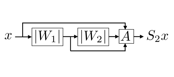
Figure 1: An illustration of the IGT with $N=2$.

The operator $A$ is chosen non negative and of norm 1. The following lemma will be helpful to show that $S_{N}$ does preserve the energy of a signal:

Lemma 3.1.

If $\forall x>0,Ax>0$ and $\|A\|\leq 1$, then $\exists 0<C\leq 1,\forall x>0,$

$$C\|x\|\leq\|Ax\|\leq\|x\|\,.$$

Proof.

Since $\|Ax\|\leq\|x\|$, then if such $C$ exists, it satisfies $C\leq 1$. Furthermore, $\{x>0\}\cap\{\|x\|=1\}$ is compact, thus, $x\rightarrow\|Ax\|$ is minored by $C$ and reached: there exists $C,x_{0}>0,\|x_{0}\|=1$ s.t. $\|Ax_{0}\|=C>0$ by assumption on $A$. ∎

In this case, Proposition 3.2 shows that $S$ is approximatively unitary and is non-expansive.

Proposition 3.2.

For $N\in\mathbb{N}$, $S_{N}$ is non-expansive, ie, $\forall x,y$:

$$\|S_{N}x-S_{N}y\|\leq\|x-y\|\,,$$ (4)

and also:

$$\|S_{N}x\|\leq\|x\|\,.$$ (5)

Furthermore, if $\epsilon=0$, then:

$$\lim_{N\rightarrow\infty}\|S_{N}x\|=\|x\|\,.$$ (6)

Proof.

For Eq. (4), observe that one has a cascade of non-expansive operator. For Eq. (5), observe that $S_{N}0=0$. For the other side of the inequality, observe that Equation (3) leads to:

$$\|U_{n}x\|^{2}=\|AU_{n}x\|^{2}+\|U_{n+1}x\|^{2}$$ (7)

Thus, a simple sum leads to:

$$\sum_{n=0}^{N}\|AU_{n}x\|^{2}+\|U_{N+1}x\|^{2}=\|x\|^{2}\,,$$

and from Lemma 3.1, $\|U_{N}x\|^{2}\leq(1-C^{2})^{N}\|x\|^{2}\rightarrow 0$ allows to conclude.

∎

We will now discuss the specific setting of Interferometric Transforms defined over graphs $\mathcal{G}$.

3.2 Recovering a Fourier basis

The goal of this section is to introduce our complex operator which is equivalent to a Fourier Transform designed specifically for a graph. Here, we will consider signals whose coordinate’s topology is organized by a graph $\mathcal{G}$, with $2d+1$ nodes and we name its corresponding Laplacian operator $\mathcal{L}$. Without loss of generality, we consider graphs with a single component, the extension to more components being natural by considering each sub-component individually. We write the orthogonal diagonalization basis of $\mathcal{L}$: $\{e_{1},...,e_{2d+1}\}$, such that $\mathcal{L}e_{2d+1}=0$. In our applications, $e_{2d+1}=(1,...,1)$ and a typical averaging $A$ that we will use, corresponds to:

$$Ax=\langle x,e_{2d+1}\rangle\,.$$

This is a consistant choice with Lemma 3.1. Note that we need to make an arbitrary choice of basis at the moment that one eigenvalue is of multiplicity larger than 1. As discussed in the introduction, the indexes $\{1,...,2d+1\}$ of the basis lacks structure, meaning that the order of the eigenvectors does not reflect the actual geometry of $\mathcal{L}$. However, standard approaches (Hammond et al., 2011) sort eigenvectors according to the amplitude of their eigenvalues and they employ this topology: here, we propose a rather different approach which behaves well in constant curvature settings. Our objective will be to pair basis’ atoms according to the smoothness of their envelope. This will be analogous to form Hilbert pairs (Krajsek & Mester, 2007), which corresponds to a pairing of the elements of the basis $\{e_{1},...,e_{2d}\}$ in order to design an analytic representation (Johansson, 1999). Well localized representations using Hilbert pairs have typically a smooth modulus (Oyallon et al., 2018a), and this analogy is a motivation for introducing this notion. To do so, for a permutation $\pi$ of $\{1,...,2d\}$, we introduce the pairing cost:

$$\begin{split}C(\pi)&=\sum_{i=1}^{d}\sum_{k=1}^{2d+1}\sqrt{e_{\pi[2i]}[k]^{2}+e_{\pi[2i-1]}[k]^{2}}\\ &=\sum_{i=1}^{d}\|e_{\pi[2i]}+\mathbf{j}e_{\pi[2i-1]}\|_{1}\,.\end{split}$$ (8)

Observe that a simple application of Cauchy-Schwartz inequality leads to $C(\pi)\leq d\sqrt{2d+1}$. We propose to find the permutation $\pi^{*}$ such that:

$$C(\pi^{*})=\max_{\pi}C(\pi)\,.$$

Again, this problem aims at finding permutations such that pairs of eigen vectors have a complex envelope which maximizes the energy along the span of $A$. Observe that this loss can be written as a separable sum of 2-entries losses. In this case, an exact solution can be obtained via a Blossom algorithm (Edmonds, 1965) which runs in polynomial time. Note that this algorithm combined with the eigen-decomposition procedure needs to be computed once, and it leads to a computational complexity of $\mathcal{O}(d^{3})$ in the worst case scenario. We then consider the matrix $\mathcal{F}=\{\mathcal{F}_{i}\}_{i\leq 2d+1}$ whose columns are defined by $\forall 1\leq i\leq d,$

$$\begin{cases}\mathcal{F}_{i}&=e_{\pi^{*}[2i]}+\mathbf{j}e_{\pi^{*}[2i-1]}\,,\\ \mathcal{F}_{2d+1-i}&=e_{\pi^{*}[2i]}-\mathbf{j}e_{\pi^{*}[2i-1]}\,,\\ \mathcal{F}_{2d+1}&=e_{2d+1}\,.\end{cases}$$ (9)

Observe that if $i\leq d$, then $\overline{\mathcal{F}_{i}}=\mathcal{F}_{2d+1-i}\in\mathbb{C}^{2d+1}$. We can then state the following proposition:

Proposition 3.3.

The matrix $\mathcal{F}$ is unitary on $\mathbb{C}^{2d+1}$.

Proof.

For simplicity, assume $\pi^{*}[i]=i$. Then, let $i$ s.t. $i\leq d$. Assume first that $j\leq d,j\neq i$, then $e_{2i}\perp e_{2j},e_{2i}\perp e_{2j-1},e_{2i-1}\perp e_{2j},e_{2i-1}\perp e_{2j-1}$, thus $\mathcal{F}_{i}\perp\mathcal{F}_{j}$ and also $\mathcal{F}_{i}\perp\overline{\mathcal{F}_{j}}$. Finally if $j=2d+1-i$,

$$\langle\mathcal{F}_{i},\overline{\mathcal{F}_{i}}\rangle =\langle e_{2i}+\mathbf{j}e_{2i-1},e_{2i}-\mathbf{j}e_{2i-1}\rangle=\|e_{2i}\|^{2}-\|e_{2i-1}\|^{2}$$

$$=0$$

∎

For illustration purpose, consider the graph $\mathcal{G}$ of a grid of length $2d+1$ with periodic boundary condition, an eigenbasis of its discrete Laplacian is clasically given, for $k\leq d,m\leq 2d+1$, by:

$$e_{2k-1}[m]=\sqrt{\frac{1}{2d+1}}\cos(\frac{\pi}{2d+1}(m-\frac{1}{2})2k)\,,$$ (10)

$$e_{2k}[m]=\sqrt{\frac{1}{2d+1}}\sin(\frac{\pi}{2d+1}(m-\frac{1}{2})2k)\,,$$ (11)

$$e_{2d+1}[m]=\frac{1}{\sqrt{2d+1}}\,.$$ (12)

In this case, we have the following lemma to derive the optimal pairing $\pi^{*}$:

Lemma 3.4.

An optimal permutation $\pi^{*}$ is given by $\pi^{*}[n]=n$.

Proof.

Introducing $Ax=\frac{1}{\sqrt{2d+1}}\sum_{m}x[m]$, from Cauchy Schwartz, under the constraint $\|x\|=1$, $Ax$ is maximal iff $x[m]=1,\forall m$. This is in particular true for $|x|[m]\triangleq|x[m]|$ if $x[m]=e^{\mathbf{j}\omega m}$ for some $\omega\in\mathbb{R}$, which is achieved by the pairing proposed in this Lemma. ∎

In this case, $\mathcal{F}_{i}[m]=\sqrt{\frac{1}{2d+1}}e^{\mathbf{j}\frac{\pi}{2d+1}(m-\frac{1}{2})2i},i\leq d$. This thus justifies the terminology Fourier Transform for $\mathcal{F}$ (up to a phase multiplication) as one can recover the Discrete Fourier Transform: our method has a natural interpretation in the Euclidean case. Pairing those eigen-vectors allows to introduce an asymetry between the real and imaginary part of our spectral operator, which will be useful and necessary for learning a complex unitary operator, that we discuss in the next section.

3.3 Specifying the isometry layer per layer

3.3.1 An energy preserving procedure

We now describe our objective for specifying each operator $W_{n}$ at order $n$. The graph filtering operators $W_{n}$ that we consider consists of $K$ filters, meaning that the eigenvalues $\{\hat{W}_{n}^{k}\}\subset\mathbb{C}^{2d+1},k\leq K$ of each $W_{n}^{k}$ can be derived from $\mathcal{F}$ via:

$$\mathcal{F}^{*}W_{n}^{k}\mathcal{F}=\text{diag}(\hat{W}_{n}^{k}),\forall k\leq K\,.$$

With a slight abuse of notations when non-ambiguous, we might write $\text{diag}(\hat{W}_{n}^{k})$ as $\hat{W}_{n}^{k}$. Let us write $x_{1},...,x_{p},...\in\mathbb{R}^{Q\times(2d+1)}$ our data points, where $Q\in\mathbb{N}$ is the number of input channels. For a signal $z$, consider the loss:

$$\ell(W,z)=\|(\mathbf{I}-A)z\|^{2}-\|A|Wz|\|^{2}\,.$$

If $W$ is an isometry, this quantifies the energy preserved after an averaging $A$. We will only consider operators which are 1-Lipschitz and diagonalized by $\mathcal{F}$, thus we consequently introduce:

$$\mathcal{C}=\{W;\|\{W,A\}\|\leq 1,\mathcal{F}^{*}W^{k}\mathcal{F}=\text{diag}(\hat{W}^{k}),\forall k\}\,.$$ (13)

Our operator $W_{n}$ will be specified by the following minimization of the empirical risk $L$:

$$W_{n}\triangleq\arg\min_{W\in\mathcal{C}}\sum_{p}\ell(W,U_{n}x_{p})=\arg\min_{W\in\mathcal{C}}L(W)\,.$$ (14)

Appendix A proves that $L$ is concave in $W$, and is positive if $\|\{W,A\}\|\leq 1$. It is very similar to a Procrustes problem (Schönemann, 1966). Concave minimization has been well studied, and a global solution of a concave minimization over a convex set lays in the extremal points of this convex set (Horst, 1984; Rockafellar, 1970; Pardalos & Rosen, 1986). The next proposition characterizes the extremal point of $\mathcal{C}$, whose proof is defered to the Appendix.

Proposition 3.5.

Let $\mathcal{S}$ the extremal points of $\mathcal{C}$, then $\mathcal{S}\subset\{W,\|Wx\|=\|(\mathbf{I}-A)x\|,\forall x\in\mathbb{R}^{2d+1}\}$.

The Figure 2 represents the spectrum of an operator $W$ learned from the small natural images of CIFAR-10. Remarkably, this operator is analytic, meaning that half of the frequency plane is set to 0 (up to a per-filter central symetry). This is natural because the analytic part of a filter is known to provide a smoother envelope, which is better captured by a low-pass filtering (Mallat, 1999). In the settings of Oyallon et al. (2018a), this is quantified. Note also that the filters are localized and smooth in frequency, which indicates that the learned filters have efficiently used the topology of the frequency domain, without explicitely incorporating any specific a priori.

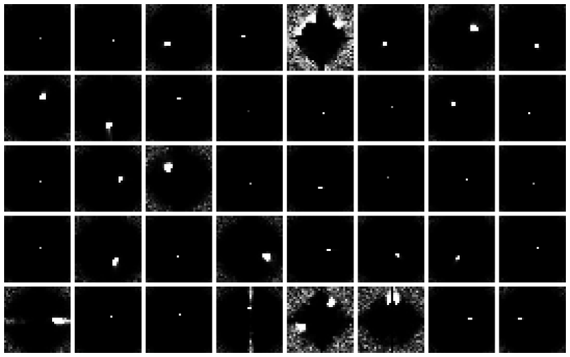
Figure 2: Spectral filters’s modulus $|\hat{W}^{k}_{1}|$ of a first order learned operator. The 0 frequency corresponds to the center. An approximatively analytic transform is obtained by solving Eq. (14) for small CIFAR-10 natural images. Observe that the filters are well localized with various frequency bandwidths, and most of them are analytic. Some filters have some noisy high frequencies, which are mainly due a poor conditioning: indeed signals’ energy is concentrated in a disk around the central frequency.

For a general graph, the topology of the frequency index is in general unknown, meaning that designing an analytic operator is challenging. On the other hand, our criterion should enforce filters which have a smooth modulus, i.e., which maximize the energy of the envelope $|Wx|$ along the span of $A$. In the next section, we discuss how to optimize Eq. (14).

3.3.2 A projected gradient method

We propose to minimize Eq. (14) by a projected gradient descent as derived in (Hager et al., 2016). Obtaining a global minimizer is a difficult task as explained in Horst (1984). In order to define our projection, we introduce a Littlewood-Paley identity (Stein, 1970) $\Gamma$, related to $W$ defined by:

$$\begin{cases}\Gamma_{i}=\sum_{k=1}^{K}|\hat{W}^{k}[2d+1-i]|^{2}+|\hat{W}^{k}[i]|^{2}\,,i\leq 2d\,,\\ \Gamma_{2d+1}=2\sum_{k=1}^{K}|\hat{W}^{k}[2d+1]|^{2}\,,\end{cases}$$

as well as $\Lambda$ related to $\mathbf{I}-A$:

$$\begin{cases}\Lambda_{i}=2-|\hat{A}[i]|^{2}-|\hat{A}[2d+1-i]|^{2}\,,i\leq 2d\,,\\ \Lambda_{2d+1}=2-2|\hat{A}[2d+1]|^{2}\,.\end{cases}$$

We then define the diagonal matrix $\hat{P}$, whose diagonal is:

$$\hat{P}_{i}=\begin{cases}1\text{, if }\Gamma_{i}\leq\Lambda_{i}\,,\\ \sqrt{\frac{\Lambda_{i}}{\Gamma_{i}}}\text{, otherwise.}\end{cases}$$

Then the convex projection on $\mathcal{C}$ is given filter-wise by:

$$\text{proj}(W^{k})=\mathcal{F}^{*}\hat{W}^{k}\hat{P}\mathcal{F}\,.$$

This leads to the following scheme, for a decreasing sequence of step size $\alpha_{t}$ and $L_{t}$ the loss at step $t$:

$$W^{t+1}=\text{proj}(W^{t}-\alpha_{t}\nabla_{W}L_{t}(W))\,,$$

with a random initialization $W_{0}$ such as a white noise. In our experiments, we typically use a stochastic gradient, thus the loss $L_{t}$ corresponds to the empirical loss over a randomly selected batch of samples. The next section provides numerical experiments which corroborate that we successfully optimized this operator to obtain a discriminative but smooth representation.

4 Numerical experiments

For each experiments, we combine an IGT representation with a linear SVM, as implemented by Fan et al. (2008). We select the order of the IGT such that more than 99% of the energy is captured, leading at maximum to an order 2. We systematically report state-of-the-art performances in unsupervised spectral GCN settings. We note that in all our benchmarks, typical unsupervised representations are shallow, similarly to our representation, which indicates that training deep unsupervised representations is a challenging task. The regularization of the SVM was cross-validated as $C=10^{-k},k=0,...,4$; no more than 3 runs have been done, without any intensive grid search. Also, as a sanity check, we experimented with random $\mathcal{F}$ or $W_{n}$, leading systematically to substential drops in performances.

4.1 Image classification

In each vision experiments, we consider the Laplacian obtained from a regular grid and we follow Henaff et al. (2015) combined with our Lemma 3.1: we can explicitely consider the standard 2D Discrete Fourier Transform. Note that shuffling image’s pixels (assuming that the Laplacian is shuffled consistantly) does not affect our algorithm: our method allows to recover the Euclidean grid structure without being explicitely incorporated, contrary to a 2D CNN. We limited our experiments to a single layer, because it already captures most of the signals’ energy. We compared our numerical performances against a Gabor Scattering Transform (Andreux et al., 2018) as well as a Haar Scattering Transform. In Chen et al. (2014), two settings are considered: one for which the geometry is known (2D grid), and one for which it is not (no grid). Also in Chen et al. (2014), an ensembling of models, combined with a supervised feature selection algorithm is used, as well as a Gaussian SVM. Instead, for the sake of comparison, we have re-run their code for a single model followed by a Linear SVM, which leads to a substantial drop in performances. In both settings, our operators have $K_{1}=40$ filters. The operator $W_{1}$ is learned via SGD with batch size 64, for 5 epochs. We reduced an initial learning rate of $1.0$ by $10$ at iterations 500, 1000 and 1500. Oyallon & Mallat (2015) and Bruna & Mallat (2013) found that averaging Scattering representations with a low-pass filter over a windows of length $2^{J}=2^{3}$ was optimal, thus we did not change this hyper parameter: if $\phi_{J}$ is a Gaussian filter of length $2^{J}$, we consider in those experiments:

$$Ax(u)=x\star\phi_{J}(u/2^{J})\,.$$ (15)

4.1.1 CIFAR-10

CIFAR-10 is a challenging dataset of small $32\times 32$ colored images, which consists of $5\times 10^{4}$ images for training and $10^{4}$ for testing. Table 1 reports our performances with a linear classifier. Observe that our method improves by about 10% the classification from the raw data. We also compare our work with supervised spectral methods, and we achieve similar performances without supervision. Despite incorporating more pointwise non-linearity, a Haar Transform performs substantially worse, which indicates that Haar features are not discriminative enough. Our spectral method leads to state-of-the-art performances, competitive with supervised methods. By incorporating the Euclidean domain knowledge, a Gabor Scattering outperforms by $10\%$ the IGT, and adding some additional supervision and more non-linearity leads to the state of the art on CIFAR10 (Zagoruyko & Komodakis, 2016).

Table 1: Classification accuracies on CIFAR-10. Sup. and Acc. stand respectively for Supervision and Accuracy.

Method	Depth	Sup.	Acc.
Raw data	-	$\times$	39.7
Spectral GCN
IGT (ours)	1	$\times$	52.4
Haar Scattering (no grid)	2	$\times$	46.3
(Knyazev et al., 2019)	3	$\surd$	50.6
(Such et al., 2017)	1	$\surd$	$\sim 52$
2D CNN
Gabor Scattering	1	$\times$	64.9
Haar Scattering (2D grid)	4	$\times$	43.4
(Zagoruyko & Komodakis, 2016)	40	$\surd$	94.1

4.1.2 MNIST

MNIST is a simple dataset of small $28\times 28$ images, which consists of $6\times 10^{4}$ images for training and $10^{4}$ for testing. Table 2 reports the accuracy of our method. Again, our method outperforms unsupervised spectral representations: for instance, IGT outperforms (Zou & Lerman, 2019) which defines a Scattering Transform based on graph wavelets. Adding some supervisions, such as in Defferrard et al. (2016b), allows to obtain competitive performances with spatial convolutional methods (Bruna & Mallat, 2013).

Table 2: Classification accuracies on MNIST.

Method	Depth	Sup.	Acc.
Raw data	-	$\times$	93.8
GCN
IGT (ours)	1	$\times$	96.1
(Zou & Lerman, 2019)	2	$\times$	95.6
Haar Scattering (no grid)	6	$\times$	82.3
(Defferrard et al., 2016b)	2	$\surd$	99.1
2D CNN
Haar Scattering (2D grid)	4	$\times$	88.6
Gabor Scattering	1	$\times$	98.6
(Defferrard et al., 2016b)	2	$\surd$	99.3

4.2 Action prediction

We now consider several 3D skeletons datasets, whose objective is to predict an action from a sequence of frame. For each dataset, a (handcrafted) skeleton represented as a graph is provided, based on human body connectivity, whose nodes are the coordinates of some human body parts (not images). Here, we preprocess our datasets using the representation proposed by Mazari & Sahbi (2019), which consists of a temporal barycenter of each node’s coordinates taken along non-overlapping windows of equal time length. We note that our goal is not to propose a new better pre-processing method than the other works we compared to, yet to improve the initial features, thus we reported the raw data accuracy.

4.2.1 SBU

Eeach SBU sample describes a two person interaction, and SBU contains 230 sequences and 8 classes (6,614 frames). The corresponding graph has 30 nodes. The accuracy is reported as the mean of the accuracies of a 5-fold procedure. We used an order 2 IGT, with $K_{1}=K_{2}=30$ filters for each operator. We train our operators for 5 epochs, with a batch size of 64, an initial learning rate of 1.0, dropped by 10 at the iterations 10, 20 and 30. Table 3 reports the accuracy of various supervised and unsupervised method on SBU. An IGT improves by about 2% a linear classifier on the raw data. Furthermore, our method achieves similar performances compared to supervised methods, while outperforming unsupervised representations.

Table 3: Accuracies on SBU, via a standard 5-fold procedure.

Method	Depth	Acc.
Raw data	-	92.7
Unsupervised
IGT (ours)	1	91.3$\pm 1.0$
IGT (ours)	2	94.5$\pm 1.0$
(Kacem et al., 2018)	-	93.7
Supervised
(Wu et al., 2019a)	1	96.0
(Mazari & Sahbi, 2019)	1	98.6

4.2.2 NTU

NTU is a challenging dataset for large scale human action analysis (Shahroudy et al., 2016), with 60 different classes and 56880 samples, corresponding to 40 subjects and 80 different views. The corresponding graph has 50 nodes. Two procedures allow to report the accuracy. In cross-subject evaluation, 40 subjects are split into training and testing groups, consisting of 20 subjects such that the training and testing sets have respectively 40,320 and 16,560 samples. For cross-view evaluation, the samples are split according to different cameras view, such that the training and testing sets have respectively 37,920 and 18,960 samples.

We use $K_{1}=10$ and $K_{2}=5$ filters respectively for our two learned operators. We trained via SGD our representation, with a batch size of 64, an initial learning rate of $1.0$ being dropped by $10$ at iterations 100, 200 and 300. Table 4 reports the accuracies for various unsupervised and supervised methods. First, observe that our method improves by about 30% a linear SVM trained on the raw features. It also outperforms all the unsupervised methods, yet a sigificant gap of 30% exists with supervised algorithm.

Here, we note that a global invariant to permutations was not required, thus we did not average our representation. In this case, a linear invariant is obtained from a linear SVM, which can freely adjust the degree of invariance to the supervised task which is considered, yet it leads to an extra-computational cost. Table 5 corresponds to an ablation of our method and indicates that here, not averaging our representation improves accuracies. Note also that in this case, first and second orders perform similarly: it indicates that the second order doesn’t recover more informative attributes yet this doesn’t invalidate any claims done. It also leads to a substential increasing of dimension. However, with an averaging, the second order brings a significant improvement over the first order because it recovers more information. Without averaging our representation, the accuracies vary by less than 1%.

Table 4: Classification accuracies on NTU, with a final linear classifier.

Method	Depth	View	Sub
Raw data	-	22.9	31.9
Unsupervised
IGT (ours)	1	54.6	60.5
IGT (ours)	2	55.6	59.9
(Evangelidis et al., 2014)	2	41.4	38.6
(Vemulapalli et al., 2014)	-	52.8	50.1
Supervised
(Li et al., 2019)	$\geq 2$	90.1	96.4

Table 5: Ablation experiments on NTU, with IGT.

Order	Averaging	View	Sub
1	$\surd$	39.7	44.0
2	$\surd$	49.3	52.9
1	$\times$	54.6	60.5
2	$\times$	55.6	59.9

4.3 Community detection

We reproduce the experiments of Gama et al. (2019) using their provided source code, and we compare our representation with a Graph Scattering Transform (GST) using various mother wavelets. In all our experiments, we used a single order IGT, and our operator is learned with a SGD with constant step size of $10^{-3}$ and batch size of 64. We followed the same evaluation procedure as Gama et al. (2019). Our experiments suggest that selecting a linear operator according to a smoothness criterion can improve the numerical performances compared to a wavelet transform, which is stable to deformations.

4.3.1 Authorship attribution

This dataset consists of a graph with 188 nodes representing a bag-of-words for some collection of texts. The objective is to decide if a writer is the author of a given text. The benchmarking of this dataset consists of reporting the accuracy given a number of training sample. Observe on Figure 3, that IGT systematically outperforms Gama et al. (2019) for each training size.

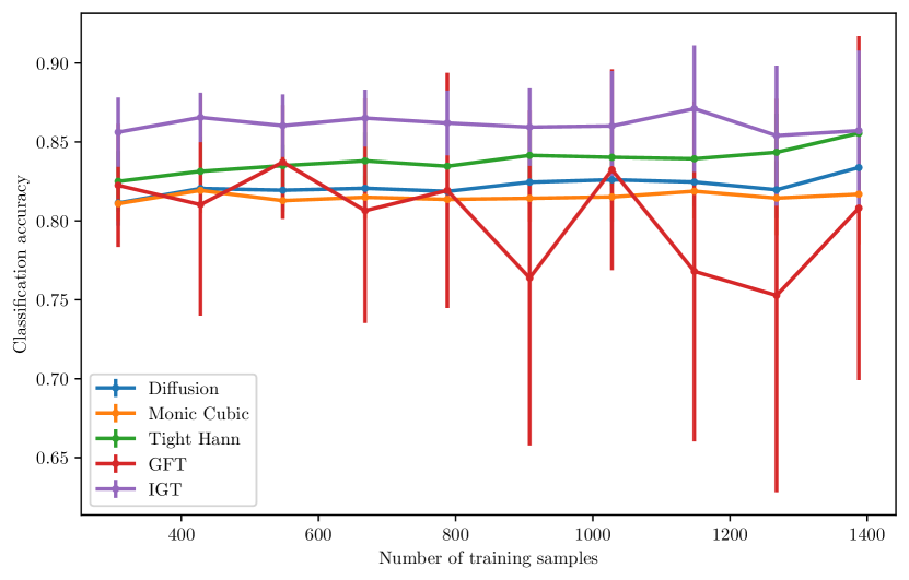
Figure 3: Authorship attribution. We compare our IGT with various mother wavelets proposed in Gama et al. (2018). The accuracy is a function of the number of training samples.

4.3.2 Facebook graph

The dataset consists of a synthetic 234 nodes graph modeling some Facebook interactions. A diffusion process is initiated at some node, and the objective is to determine which community this original node belongs to. In order to make this dataset challenging, a fraction of the edge is dropped and the classification accuracy is reported for various probability of edge failure. $2\times 10^{3}$ points are used from training and $2\times 10^{2}$ points for testing. Figure 4 reports our performances. Obtaining 100% on the test set, our method solves this dataset, which clearly outperforms GST introduced in Gama et al. (2018) for each wavelet family.

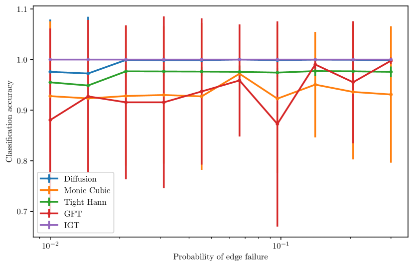
Figure 4: Facebook graph. We compare our IGT with various mother wavelets proposed in Gama et al. (2018). The classification accuracy is reported as well as its variance, as a function of the fraction of edges dropped.

5 Conclusion

In our work, we introduced the Inteferometric Graph Transform, which is an unsupervised, generic and interpretable representation that is guaranteed to obtain smooth features. We introduced a complex unitary transform for graphs analog to a Fourier transform. Thanks to our concave optimization procedure motivated by invariance and energy preservation considerations, we obtain performances at the level of the state of the art on many various complex benchmarks. In vision settings, we observe that our method obtains analytic and well structured operators, which is surprising.

In a future work, we would like to extend this method to hybrid models, combining IGT and deep supervised GCN models, as done in Oyallon et al. (2018b, 2017) for natural images on a regular grid. Another question which is still open, is to understand if it would be possible to provide a low dimensional mapping (Jacobsen et al., 2017) of our spectral basis, similar to the index of a $N$-dimensional Fourier basis.

Acknowledgement:

The author would like to thank Mathieu Andreux, Eugene Belilovsky, Bogdan Cirstea, Thomas Pumir, John Zarka for proofreading this manuscript, as well as Lucas Silve and Ahmed Mazari for helpful discussions related to the experiments. The author was supported by a GPU donation from NVIDIA.

Appendix A Proof that $L$ is concave and positive.

We will use the notations previously introduced as well as:

$$z_{p}=U_{n}x_{p}\,.$$

As $L(W)=\sum_{p}\ell(W,z_{p})$, we will simply study $\forall z$,

$$W\rightarrow\ell(W,z)=\|(\mathbf{I}-A)z\|^{2}-\|A|Wz|\|^{2}\,.$$

Observe first that if $\|\{W,A\}\|\leq 1$, then $\|A|\leq 1$, and:

$$\|Wz\|\leq\|(\mathbf{I}-A)z\|$$

Thus,

$$\||Wz|\|\leq\|(\mathbf{I}-A)z\|$$

and:

$$\|A|Wz|\|\leq\|(\mathbf{I}-A)z\|\,.$$

Consequently, $\ell(W,z)\geq 0,\forall z,\forall W\in\mathcal{C}$. Furthermore, let $W_{1},W_{2}\in\mathcal{C}$ two operators and $0\leq\lambda\leq 1$. Then:

$$|\big{(}\lambda W_{1}+(1-\lambda)W_{2}\big{)}z|\leq\lambda|W_{1}|z+(1-\lambda)|W_{2}|z$$

where for $x\in\mathbb{R}^{n}$, $x\geq 0$ iff $x_{i}\geq 0$. If $Ax>0$ when $x>0$, then:

$$A|\big{(}\lambda W_{1}+(1-\lambda)W_{2}\big{)}z|\leq\lambda A|W_{1}|z+(1-\lambda)A|W_{2}|z|\,,$$

which implies (as all coordinates are non negative):

$$\|A|\big{(}\lambda W_{1}+(1-\lambda)W_{2}\big{)}z|\|^{2}\leq\|\lambda A|W_{1}|z+(1-\lambda)A|W_{2}|z|\|^{2}\,,$$

yet one can use the fact that $z\rightarrow\|z\|^{2}$ is convex to conclude. Thus, $W\rightarrow\ell(W,z)$ is convex in $W$.

Appendix B Proof of Proposition 3.5

Proof.

Observe that $\mathcal{F}$ linearly conjugates $\mathcal{C}$ to $\{\hat{W}\in\mathbb{C}^{(2d+1)\times K},\sum_{k=1}^{K}|\hat{W}^{k}[i]|^{2}+|W^{k}[2d+1-i]|^{2}+|\hat{A}[i]|^{2}+|\hat{A}[2d+1-i]|^{2}\leq 1,\forall i\leq d,\sum_{k=1}^{K}|W^{k}[2d+1]|^{2}+|\hat{A}[2d+1]|^{2}\leq 1\}$. The extremal points of the latter are simply $\mathcal{S}^{\prime}=\{\hat{W}\in\mathbb{C}^{(2d+1)\times K},\sum_{k=1}^{K}|\hat{W}^{k}[i]|^{2}+|W^{k}[2d+1-i]|^{2}+|\hat{A}[i]|^{2}+|\hat{A}[2d+1-i]|^{2}=1,\forall i\leq d,\sum_{k=1}^{K}|W^{k}[2d+1]|^{2}+|\hat{A}[2d+1]|^{2}=1\}$, which is conjugated by $\mathcal{F}^{*}$ to $\mathcal{S}$. But $\mathcal{S}^{\prime}$ corresponds to the spectrum of an isometry, leading to the conclusion. ∎

References

- Andreux et al. (2018) Andreux, M., Angles, T., Exarchakis, G., Leonarduzzi, R., Rochette, G., Thiry, L., Zarka, J., Mallat, S., Andén, J., Belilovsky, E., et al. Kymatio: Scattering transforms in python. arXiv preprint arXiv:1812.11214, 2018.
- Belilovsky et al. (2017) Belilovsky, E., Kastner, K., Varoquaux, G., and Blaschko, M. B. Learning to discover sparse graphical models. In Proceedings of the 34th International Conference on Machine Learning-Volume 70, pp. 440–448. JMLR. org, 2017.
- Belilovsky et al. (2018) Belilovsky, E., Eickenberg, M., and Oyallon, E. Greedy layerwise learning can scale to imagenet. arXiv preprint arXiv:1812.11446, 2018.
- Belilovsky et al. (2019) Belilovsky, E., Eickenberg, M., and Oyallon, E. Decoupled greedy learning of cnns. arXiv preprint arXiv:1901.08164, 2019.
- Bronstein et al. (2017) Bronstein, M. M., Bruna, J., LeCun, Y., Szlam, A., and Vandergheynst, P. Geometric deep learning: going beyond euclidean data. IEEE Signal Processing Magazine, 34(4):18–42, 2017.
- Bruna & Mallat (2013) Bruna, J. and Mallat, S. Invariant scattering convolution networks. IEEE transactions on pattern analysis and machine intelligence, 35(8):1872–1886, 2013.
- Bruna et al. (2013) Bruna, J., Zaremba, W., Szlam, A., and LeCun, Y. Spectral networks and locally connected networks on graphs. arXiv preprint arXiv:1312.6203, 2013.
- Carey (2017) Carey, C. Graph construction for manifold discovery. 2017.
- Chen et al. (2014) Chen, X., Cheng, X., and Mallat, S. Unsupervised deep haar scattering on graphs. In Advances in Neural Information Processing Systems, pp. 1709–1717, 2014.
- De Cao & Kipf (2018) De Cao, N. and Kipf, T. Molgan: An implicit generative model for small molecular graphs. arXiv preprint arXiv:1805.11973, 2018.
- Defferrard et al. (2016a) Defferrard, M., Bresson, X., and Vandergheynst, P. Convolutional neural networks on graphs with fast localized spectral filtering. In Lee, D. D., Sugiyama, M., Luxburg, U. V., Guyon, I., and Garnett, R. (eds.), Advances in Neural Information Processing Systems 29, pp. 3844–3852. Curran Associates, Inc., 2016a. URL http://papers.nips.cc/paper/6081-convolutional-neural-networks-on-graphs-with-fast-localized-spectral-filtering.pdf.
- Defferrard et al. (2016b) Defferrard, M., Bresson, X., and Vandergheynst, P. Convolutional neural networks on graphs with fast localized spectral filtering. In Advances in neural information processing systems, pp. 3844–3852, 2016b.
- Edmonds (1965) Edmonds, J. Paths, trees, and flowers. Canadian Journal of Mathematics, 17:449–467, 1965. doi: 10.4153/CJM-1965-045-4.
- Evangelidis et al. (2014) Evangelidis, G., Singh, G., and Horaud, R. Skeletal quads: Human action recognition using joint quadruples. In 2014 22nd International Conference on Pattern Recognition, pp. 4513–4518. IEEE, 2014.
- Fan et al. (2008) Fan, R.-E., Chang, K.-W., Hsieh, C.-J., Wang, X.-R., and Lin, C.-J. Liblinear: A library for large linear classification. Journal of machine learning research, 9(Aug):1871–1874, 2008.
- Gama et al. (2018) Gama, F., Ribeiro, A., and Bruna, J. Diffusion scattering transforms on graphs. arXiv preprint arXiv:1806.08829, 2018.
- Gama et al. (2019) Gama, F., Ribeiro, A., and Bruna, J. Stability of graph scattering transforms. In Advances in Neural Information Processing Systems, pp. 8036–8046, 2019.
- Gao & Ji (2019) Gao, H. and Ji, S. Graph u-nets. arXiv preprint arXiv:1905.05178, 2019.
- Gao et al. (2019) Gao, H., Chen, Y., and Ji, S. Learning graph pooling and hybrid convolutional operations for text representations. In The World Wide Web Conference, pp. 2743–2749. ACM, 2019.
- Hager et al. (2016) Hager, W. W., Phan, D. T., and Zhu, J. Projection algorithms for nonconvex minimization with application to sparse principal component analysis. Journal of Global Optimization, 65(4):657–676, 2016.
- Hamilton et al. (2017) Hamilton, W., Ying, Z., and Leskovec, J. Inductive representation learning on large graphs. In Advances in Neural Information Processing Systems, pp. 1024–1034, 2017.
- Hammond et al. (2011) Hammond, D. K., Vandergheynst, P., and Gribonval, R. Wavelets on graphs via spectral graph theory. Applied and Computational Harmonic Analysis, 30(2):129–150, 2011.
- Henaff et al. (2015) Henaff, M., Bruna, J., and LeCun, Y. Deep convolutional networks on graph-structured data. arXiv preprint arXiv:1506.05163, 2015.
- Horst (1984) Horst, R. On the global minimization of concave functions. Operations-Research-Spektrum, 6(4):195–205, 1984.
- Jacobsen et al. (2017) Jacobsen, J.-H., Oyallon, E., Mallat, S., and Smeulders, A. W. Multiscale hierarchical convolutional networks. arXiv preprint arXiv:1703.04140, 2017.
- Johansson (1999) Johansson, M. The hilbert transform. 1999.
- Kacem et al. (2018) Kacem, A., Daoudi, M., Amor, B. B., Berretti, S., and Alvarez-Paiva, J. C. A novel geometric framework on gram matrix trajectories for human behavior understanding. IEEE transactions on pattern analysis and machine intelligence, 2018.
- Kampffmeyer et al. (2019) Kampffmeyer, M., Chen, Y., Liang, X., Wang, H., Zhang, Y., and Xing, E. P. Rethinking knowledge graph propagation for zero-shot learning. In Proceedings of the IEEE Conference on Computer Vision and Pattern Recognition, pp. 11487–11496, 2019.
- Kipf & Welling (2016) Kipf, T. N. and Welling, M. Variational graph auto-encoders. arXiv preprint arXiv:1611.07308, 2016.
- Knyazev et al. (2019) Knyazev, B., Lin, X., Amer, M. R., and Taylor, G. W. Image classification with hierarchical multigraph networks. arXiv preprint arXiv:1907.09000, 2019.
- Krajsek & Mester (2007) Krajsek, K. and Mester, R. A unified theory for steerable and quadrature filters. In Advances in Computer Graphics and Computer Vision, pp. 201–214. Springer, 2007.
- Lee et al. (2019) Lee, J., Lee, I., and Kang, J. Self-attention graph pooling. arXiv preprint arXiv:1904.08082, 2019.
- Li et al. (2019) Li, M., Chen, S., Chen, X., Zhang, Y., Wang, Y., and Tian, Q. Symbiotic graph neural networks for 3d skeleton-based human action recognition and motion prediction, 2019.
- Li et al. (2018) Li, Q., Han, Z., and Wu, X.-M. Deeper insights into graph convolutional networks for semi-supervised learning. In Thirty-Second AAAI Conference on Artificial Intelligence, 2018.
- Luzhnica et al. (2019) Luzhnica, E., Day, B., and Lio, P. Clique pooling for graph classification. arXiv preprint arXiv:1904.00374, 2019.
- Mallat (1999) Mallat, S. A wavelet tour of signal processing. Elsevier, 1999.
- Mallat (2010) Mallat, S. Recursive interferometric representation. 2010.
- Mallat (2012) Mallat, S. Group invariant scattering. Communications on Pure and Applied Mathematics, 65(10):1331–1398, 2012.
- Mallat & Waldspurger (2013) Mallat, S. and Waldspurger, I. Deep learning by scattering. arXiv preprint arXiv:1306.5532, 2013.
- Mazari & Sahbi (2019) Mazari, A. and Sahbi, H. Mlgcn: Multi-laplacian graph convolutional networks for human action recognition. BMVC, 2019.
- NT & Maehara (2020) NT, H. and Maehara, T. Frequency analysis for graph convolution network, 2020. URL https://openreview.net/forum?id=HylthC4twr.
- Oyallon (2017) Oyallon, E. Building a regular decision boundary with deep networks. In The IEEE Conference on Computer Vision and Pattern Recognition (CVPR), July 2017.
- Oyallon & Mallat (2015) Oyallon, E. and Mallat, S. Deep roto-translation scattering for object classification. In Proceedings of the IEEE Conference on Computer Vision and Pattern Recognition, pp. 2865–2873, 2015.
- Oyallon et al. (2017) Oyallon, E., Belilovsky, E., and Zagoruyko, S. Scaling the scattering transform: Deep hybrid networks. In The IEEE International Conference on Computer Vision (ICCV), Oct 2017.
- Oyallon et al. (2018a) Oyallon, E., Belilovsky, E., Zagoruyko, S., and Valko, M. Compressing the input for cnns with the first-order scattering transform. In Proceedings of the European Conference on Computer Vision (ECCV), pp. 301–316, 2018a.
- Oyallon et al. (2018b) Oyallon, E., Zagoruyko, S., Huang, G., Komodakis, N., Lacoste-Julien, S., Blaschko, M., and Belilovsky, E. Scattering networks for hybrid representation learning. IEEE transactions on pattern analysis and machine intelligence, 41(9):2208–2221, 2018b.
- Pardalos & Rosen (1986) Pardalos, P. M. and Rosen, J. B. Methods for global concave minimization: A bibliographic survey. SIAM Review, 28(3):367–379, 1986. doi: 10.1137/1028106. URL https://doi.org/10.1137/1028106.
- Ren et al. (2019) Ren, Y., Liu, B., Huang, C., Dai, P., Bo, L., and Zhang, J. Heterogeneous deep graph infomax. arXiv preprint arXiv:1911.08538, 2019.
- Rockafellar (1970) Rockafellar, R. T. Convex analysis, volume 28. Princeton university press, 1970.
- Ruiz et al. (2020) Ruiz, L., Chamon, L. F., and Ribeiro, A. Graphon signal processing. arXiv preprint arXiv:2003.05030, 2020.
- Salha et al. (2019) Salha, G., Hennequin, R., and Vazirgiannis, M. Keep it simple: Graph autoencoders without graph convolutional networks. arXiv preprint arXiv:1910.00942, 2019.
- Schönemann (1966) Schönemann, P. H. A generalized solution of the orthogonal procrustes problem. Psychometrika, 31(1):1–10, 1966.
- Shahroudy et al. (2016) Shahroudy, A., Liu, J., Ng, T.-T., and Wang, G. Ntu rgb+ d: A large scale dataset for 3d human activity analysis. In Proceedings of the IEEE conference on computer vision and pattern recognition, pp. 1010–1019, 2016.
- Stein (1970) Stein, E. M. Topics in harmonic analysis, related to the Littlewood-Paley theory. Princeton University Press, 1970.
- Such et al. (2017) Such, F. P., Sah, S., Dominguez, M. A., Pillai, S., Zhang, C., Michael, A., Cahill, N. D., and Ptucha, R. Robust spatial filtering with graph convolutional neural networks. IEEE Journal of Selected Topics in Signal Processing, 11(6):884–896, Sep. 2017. ISSN 1941-0484. doi: 10.1109/JSTSP.2017.2726981.
- Veličković et al. (2018) Veličković, P., Fedus, W., Hamilton, W. L., Liò, P., Bengio, Y., and Hjelm, R. D. Deep graph infomax. arXiv preprint arXiv:1809.10341, 2018.
- Vemulapalli et al. (2014) Vemulapalli, R., Arrate, F., and Chellappa, R. Human action recognition by representing 3d skeletons as points in a lie group. In Proceedings of the IEEE conference on computer vision and pattern recognition, pp. 588–595, 2014.
- Wu et al. (2019a) Wu, F., Zhang, T., Souza Jr, A. H. d., Fifty, C., Yu, T., and Weinberger, K. Q. Simplifying graph convolutional networks. arXiv preprint arXiv:1902.07153, 2019a.
- Wu et al. (2019b) Wu, Z., Pan, S., Chen, F., Long, G., Zhang, C., and Yu, P. S. A comprehensive survey on graph neural networks. arXiv preprint arXiv:1901.00596, 2019b.
- Ying et al. (2018) Ying, Z., You, J., Morris, C., Ren, X., Hamilton, W., and Leskovec, J. Hierarchical graph representation learning with differentiable pooling. In Advances in Neural Information Processing Systems, pp. 4800–4810, 2018.