Deriving Bounds and Inequality Constraints Using Logical
Relations Among Counterfactuals

Abstract

Causal parameters may not be point identified in the presence of unobserved confounding. However, information about non-identified parameters, in the form of bounds, may still be recovered from the observed data in some cases. We develop a new general method for obtaining bounds on causal parameters using rules of probability and restrictions on counterfactuals implied by causal graphical models. We additionally provide inequality constraints on functionals of the observed data law implied by such causal models. Our approach is motivated by the observation that logical relations between identified and non-identified counterfactual events often yield information about non-identified events. We show that this approach is powerful enough to recover known sharp bounds and tight inequality constraints, and to derive novel bounds and constraints.

1 INTRODUCTION

Directed acyclic graphs (DAGs) are commonly used to represent causal relationships between random variables, with a directed edge from $A$ to $Y$ ($A\rightarrow Y$) representing that $A$ “directly causes” $Y$. Under the interventionist view of causality, this relationship is taken to mean that $Y$ may change if any set of variables ${\bf S}$ that includes $A$ is set, possibly contrary to fact, to values ${\bf s}$. The operation that counterfactually sets values of variables is known as an intervention and has been denoted by the $do({\bf s})$ operator in [12].

The variable $Y$ after an intervention $do(a)$ is performed is denoted $Y(a)$, and is referred to as a potential outcome, or a counterfactual random variable [10]. Distributions over counterfactuals such as $P(Y(a))$ may be used to quantify cause-effect relationships by means of a hypothetical randomized controlled trial (RCT). For example, the average causal effect (ACE) is defined as $\mathbb{E}[Y(a)]-\mathbb{E}[Y(a^{\prime})]$ and is a comparison of means in two arms of a hypothetical RCT, with the arms defined by $do(a)$ and $do(a^{\prime})$ operations.

Since counterfactuals are not observed directly in the data, assumptions are needed to link counterfactual parameters with the observed data distribution. These assumptions are provided by causal models (often represented by DAGs), which are substantively justified using background knowledge or learned directly from data [19].

Under some causal models, counterfactual distributions $P(Y(a))$ may be identified exactly (expressed as functionals of the observed data distribution) [20, 18, 6]. However, when causally relevant variables are not observed, counterfactual distributions may not be identified.

The ideal approach for dealing with non-identified parameters is additional data collection that would “expand” the observed data distribution by rendering previously unobserved variables observable, and thus a previously non-identified parameter identifiable.

If additional data collection is not possible, the alternative is to impose additional parametric assumptions on the causal model which would imply identification, or retreat to a weaker notion of identification, where the observed data distribution is used to obtain bounds on the non-identified parameter of interest. The existence of such bounds may yield substantively significant conclusions, for instance by indicating that the causal effect is present (if the corresponding parameter is bounded away from $0$).

A well known example of a causal model with a non-identified causal parameter with non-trivial bounds is the instrumental variable (IV) model [1, 9, 17]. The original sharp bounds for the causal parameter in the IV model were derived using a computationally intensive, and difficult to interpret, convex polytope vertex enumeration approach [1]. Subsequent work [13] has extended this approach to other scenarios where a counterfactual objective can be expressed as a linear function of the observed data law. These approaches are limited both by computational complexity and by the required linear form of the objective.

Bounds on causal parameters are related to inequality constraints on the observed data law implied by hidden variable DAGs, as demonstrated by the derivation of the original IV inequalities [1], and subsequent work on inequality constraints [4, 7]. The approach developed in [22] for deriving such inequality constraints is very general and is conjectured to be able to recover all constraints implied by a hidden variable DAG, but is computationally challenging to evaluate, and has no bounded running time.

In this paper, we present a new approach for deriving bounds on non-identified causal parameters that directly uses restrictions implied by a causal model, rules of probability theory, and logical relations between identified and non-identified counterfactual events. We then build on this approach to present a new class of inequality constraints on the observed data law.

The paper is organized as follows. We introduce notation and relevant concepts in Section 2. We provide an intuitive introduction to our method by re-deriving known sharp bounds in the binary IV model [1] in Section 3. In Section 4, we present results important to our approach, and provide a general algorithm for obtaining bounds on causal parameters. Section 5 demonstrates how our approach may be used to derive generalized instrumental variable inequalities, of which the original IV inequalities and Bonet’s inequalities [3] are special cases. Finally, in Section 6 we make use of these results to provide novel bounds and inequality constraints for two sample models.

2 PRELIMINARIES

We let $\mathcal{G}$ denote a DAG with a vertex set $\bf V$ such that each element of $\bf V$ corresponds to a random variable. The statistical model of $\mathcal{G}$ is the set of joint distributions $P({\bf V})$ that are Markov relative to the DAG ${\cal G}$. Specifically, it’s the set $\{P({\bf V}):P({\bf V})=\prod_{V\in{\bf V}}P(V|\operatorname{pa}_{\mathcal{G}}(V))\}$, where $\operatorname{pa}_{\mathcal{G}}(V)$ is the set of parents of $V$ in $\mathcal{G}$.

The causal model of a DAG is also a set of joint distributions, but over counterfactual random variables. A counterfactual $Y(a)$ denotes the random variable $Y$ in a counterfactual world, where $A$ is exogenously set to the value $a$.

Such a causal model can be described by a set of structural equations $\{f_{V}(\operatorname{pa}_{\mathcal{G}}(V),\epsilon_{V})\mid V\in{\bf V}\}$, where each $f_{V}$ can be thought of as a causal mechanism that maps values of $\operatorname{pa}_{\cal G}(V)$ (parents of $V$) and the exogenous noise term $\epsilon_{V}$ to a value of $V$. For a given set of values ${\bf a}$ of $\operatorname{pa}_{\cal G}(V)$, variation of $\epsilon_{V}$ yields the counterfactual random variable $V({\bf a})$ as the output of $f_{V}({\bf a},\epsilon_{V})$.

Other counterfactuals can be defined through recursive substitution [15], as follows:

$$Y({\bf a})=\begin{cases}{\bf a}_{Y}&\mbox{if }Y\in{\bf A}\\ f_{Y}(\{V({\bf a})\mid V\in\operatorname{pa}_{\mathcal{G}}(Y)\},\epsilon_{Y})&\mbox{otherwise }\end{cases}$$ (1)

This definition, following from the structural equation model view of the causal model of a DAG, allows the effects of exogenous intervention to propagate downstream to the outcome of interest. Under this view, only the noise variables in the set $\{\epsilon_{V}:V\in{\bf V}\}$ are random. The distributions of the observed data and of counterfactual random variables can be thought of as the distributions of different functions of $\{\epsilon_{V}:V\in{\bf V}\}$ as described in (1).

As a notational convention, given any set $\{Y_{1},\ldots,Y_{k}\}\equiv{\bf Y}$, and a set of treatments ${\bf A}$ set to ${\bf a}$, we will denote a set of counterfactuals $\{Y_{1}({\bf a}),\ldots,Y_{k}({\bf a})\}$ defined by (1) by the shorthand ${\bf Y}({\bf a})$. We will sometimes denote single variable events $Y({\bf a})=y$ via the shorthand $y({\bf a})$ for conciseness, similarly multivariable events ${\bf Y}({\bf a})={\bf y}$ will sometimes be denoted as ${\bf y}({\bf a})$.

One consequence of (1) is that some counterfactuals $Y({\bf a})$ only depend on a subset of values in ${\bf a}$, specifically those values that make an appearance in one of the base cases of the definition. Restrictions of this sort are sometimes called exclusion restrictions.

The recursive substitution definition above implies the following generalized consistency property, which states that for any disjoint subsets ${\bf A},{\bf B},{\bf Y}$ of ${\bf V}$,

$${\bf B}({\bf a})={\bf b}\text{ implies }{\bf Y}({\bf a},{\bf b})={\bf Y}({\bf a}).$$ (2)

If all variables ${\bf V}$ in a causal model represented by a DAG ${\cal G}$ are observed, every interventional distribution $P({\bf Y}({\bf a}))$, where ${\bf A}\subseteq{\bf V}$, ${\bf Y}\subseteq{\bf V}\setminus{\bf A}$, is identified from $P({\bf V})$ via the following functional: $\sum_{{\bf V}\setminus({\bf Y}\cup{\bf A})}\prod_{V\in{\bf V}\setminus({\bf Y}\cup{\bf A})}P(V|\operatorname{pa}_{\cal G}(V))|_{{\bf A}={\bf a}}$, known as the g-formula [16].

In practice, not all variables in a causal model may be observed. In a hidden variable causal model, represented by a DAG ${\cal G}({\bf V}\cup{\bf H})$, where no data is available on variables in ${\bf H}$, not every counterfactual distribution is identified.

Reasoning about parameter identification is often performed via an acyclic directed mixed graph (ADMG) summary of ${\cal G}({\bf V}\cup{\bf H})$ called a latent projection ${\cal G}({\bf V})$ [21]. The latent projection keeps vertices corresponding to ${\bf V}$, and adds two kinds of edges between these vertices. A directed edge ($\to$) between any $V_{i},V_{j}\in{\bf V}$ is added if there exists a directed path from $V_{i}$ to $V_{j}$ in ${\cal G}({\bf V}\cup{\bf H})$ and all intermediate vertices on the path are in ${\bf H}$. A bidirected edge ($\leftrightarrow$) between any $V_{i},V_{j}\in{\bf V}$ is added if there exists a path from $V_{i}$ to $V_{j}$ which starts with an edge into $V_{i}$, ends with an edge into $V_{j}$, has no two adjacent edges pointing into the same vertex on the path, and has all intermediate elements in ${\bf H}$. See Fig. 1 (a) and (b) for a simple example of this construction for the IV model.

If $P({\bf Y}({\bf a}))$ is identified from $P({\bf V})$ in a causal model represented by a hidden variable DAG ${\cal G}({\bf V}\cup{\bf H})$, then its identifying functional may be expressed using ${\cal G}({\bf V})$ via the ID algorithm [20]. See [14] for details.

If $P({\bf y}({\bf a}))$ is not identified from $P({\bf V})$ in a causal model given by ${\cal G}({\bf V}\cup{\bf H})$, bounds may nevertheless be placed on this distribution. Before describing our approach for obtaining bounds in full generality, we illustrate how it may be used to obtain known sharp bounds for a non-identified counterfactual probability in the binary IV model.

3 BOUNDS IN THE BINARY INSTRUMENTAL VARIABLE MODEL

The instrumental variable model is represented graphically in Fig. 1 (a), with its latent projection shown in Fig. 1 (b). We are interested in the counterfactual probability $P(y(a))$, which is known not to be identified without parametric assumptions. In this section, we demonstrate that known sharp bounds on $P(y(a))$ can be recovered by reasoning causally about the structure of this graph and the associated counterfactual distributions.

Figure 1: (a) The classic instrumental variable model, and (b) its latent projection.

The Instrumental Variable Thought Experiment

We consider the binary IV model in Fig. 1 (a) in the setting of clinical trials with non-compliance. We interpret $Z$ to indicate treatment assignment, $A$ to indicate treatment actually taken, and $Y$ to indicate a clinical outcome of interest. Unobserved factors, such as personality traits, may influence both treatment decision and outcome, and thus act as confounders.

Suppose we intervene to assign some subject to treatment arm $z$. We observe that after this intervention, our subject takes treatment $a$ and has outcome $y$. Thus, in this subject, we observe the event $A(z)=a\land Y(z)=y$.

Now suppose we are interested in intervening directly on treatment for the same subject. We would like to set $A=a$, leaving $Z$ (arm assignment) to the physician’s choice. Under the model, the outcome $Y$ depends only on $A$ and the noise term $\epsilon_{Y}$, representing in this case subject-specific personality traits. Because these traits are unchanged by intervention on $A$ or $Z$, and $A$ is set to the same value it took under our first intervention, we must conclude that under this second intervention we would observe the same outcome as under the first, denoted by the event $Y(a)=y$.

This thought experiment demonstrates that an event in one hypothetical world, under one intervention, can imply an event under another intervention. We call this phenomenon “cross-world implication,” and it is formalized in proposition 2. We now develop the intuition further to recover sharp bounds for the IV model with binary random variables.

Sharp Bounds in the Binary IV Model

In the following derivation of sharp bounds for $P(y(a))$ in the binary IV model, we will denote values $1$ for all variables by lower case (e.g. $a$), and values $0$ by a lower case with a bar (e.g. $\bar{a}$).

Our strategy will be to partition the event $Y(a)=y$ into smaller, more manageable events:

$$A(\bar{z}) =a\land Y(\bar{z})=y$$ (3)

$$A(\bar{z})=\bar{a}\land A(z) =a\land Y(z)=y$$ (4)

$$A(\bar{z})=\bar{a}\land A(z) =\bar{a}\land Y(a)=y.$$ (5)

Note that events in (4) and (5) are related to the compliers and never-takers principal strata [5].

To see that these events form a partition (i.e. are mutually exclusive and exhaustive) of the event $Y(a)=y$, we first observe that by the exclusion restriction in the model, and generalized consistency, $Y(\bar{z})$ and $Y(z)$ in equations (3) and (4) respectively will be equal to $Y(a)$. Then we can see that (3) covers the portion of $Y(a)=y$ where $A(\bar{z})=a$, (4) covers the portion where $A(\bar{z})=\bar{a}\land A(z)=a$, and (5) covers the portion where $A(\bar{z})=A(z)=\bar{a}$.

Because these events partition $Y(a)=y$, the sum of their probabilities will be equal to $P(Y(a)=y)$, and a sum of lower-bounds on their probabilities will yield a lower bound on $P(Y(a)=y)$. A general form of partitions of this sort for counterfactual events under models with an exclusion restriction will be given in Proposition 5.

The event (3) represents a single world event with an identified probability, that therefore does not need to be bounded. We will see that we can recover sharp bounds without bounding the probability of (5).

We therefore turn our attention to event (4). This event can be understood as a conjunction of events in two worlds. First, $A(\bar{z})=\bar{a}$ in the world in which $Z$ is set to $\bar{z}$. Then, $A(z)=a\land Y(z)=y$ in the world in which $Z$ is set to $z$. As a cross world event, (4) does not have an identified density. Our goal will be to provide lower bounds for this event that are identified.

First, we find some event $E_{1}$ under the intervention $Z=\bar{z}$ that entails $A(\bar{z})=\bar{a}$. We can then identify outcomes under the (conflicting) intervention $Z=z$ that are compatible with $E_{1}$, i.e. that would not be ruled out by observing $E_{1}$ under intervention $Z=\bar{z}$. We denote such events by $\psi_{z}(E_{1})$. Now, by definition:

$$P(E_{1} )-P(E_{1},\neg\big{(}A(z)=a\land Y(z)=y\big{)})$$ (6)

$$=P(E_{1},\big{(}A(z)=a\land Y(z)=y\big{)}).$$

We note that $E_{1}\implies\psi_{z}(E_{1})$ by construction, as $E_{1}$ rules out all outcomes in the sample space not in $\psi_{z}(E_{1})$, so $P(E_{1},\neg\big{(}A(z)=a\land Y(z)=y\big{)})$ is bounded from above by $P(\psi_{z}(E_{1}),\neg\big{(}A(z)=a\land Y(z)=y\big{)})$.

Substituting this bound into equation (6) yields:

$$P(E_{1})- P(\psi_{z}(E_{1}),\neg\big{(}A(z)=a\land Y(z)=y\big{)})$$

$$\leq P(E_{1},\big{(}A(z)=a\land Y(z)=y\big{)}).$$ (7)

Because $E_{1}$ was chosen to entail $A(\bar{z})=\bar{a}$, the probability of event (4) is bounded from below by $P(E_{1},\big{(}A(z)=a\land Y(z)=y\big{)})$. Therefore by equation (7), the probability of event (4) is also bounded from below by:

$$P(E_{1})-P(\psi_{z}(E_{1}),\neg\big{(}A(z)=a\land Y(z)=y\big{)}).$$ (8)

Through exactly analogous reasoning, we can obtain another lower bound on the probability of event (4) by starting with some event $E_{2}$ under $Z=z$ that entails $A(z)=a\land Y(z)=y$:

$$P(E_{2})-P(\psi_{\bar{z}}(E_{2}),\neg\big{(}A(\bar{z})=\bar{a}\big{)}).$$ (9)

To apply these bounds, we must select events that satisfy the criteria for $E_{1}$ and $E_{2}$. We start by examining potential events $E_{1}$. We note that there are only three options: $A(\bar{z})=\bar{a}$, $A(\bar{z})=\bar{a}\land Y(\bar{z})=\bar{y}$, and $A(\bar{z})=\bar{a}\land Y(\bar{z})=y$. It turns out that we need only consider the latter two of these (see Proposition 10 in Appendix C).

First, we take $E_{1}$ to be $A(\bar{z})=\bar{a}\land Y(\bar{z})=\bar{y}$. Then we note $\psi_{z}(A(\bar{z})=\bar{a}\land Y(\bar{z})=\bar{y})$ is:

$$\big{(}A(z) =\bar{a}\land Y(z)=\bar{y}\big{)}$$

$$\lor\leavevmode\nobreak\ \big{(}A(z) =a\land Y(z)=\bar{y}\big{)}$$

$$\lor\leavevmode\nobreak\ \big{(}A(z) =a\land Y(z)=y\big{)}.$$

The only outcome under the intervention $Z=z$ excluded from this event is $A(z)=\bar{a}\land Y(z)=y$. Any subject who experienced this event could not have experienced $A(\bar{z})=\bar{a}\land Y(\bar{z})=\bar{y}$, due to the exclusion restriction in the IV model.

According to (8), to obtain a bound we will need to subtract from the mass of $E_{1}$ the mass of the portion of $\psi_{z}(E_{1})$ where $A(z)=a\land Y(z)=y$ does not hold. This will be the mass of the first two events in the disjunction above.

Using this value of $E_{1}$, we therefore obtain the following lower bound on the probability of (4):

$$P(A(\bar{z})=\bar{a},Y(\bar{z})=\bar{y})-$$ (10)

$$P(\big{(}A(z)=\bar{a}, Y(z)=\bar{y}\big{)}\lor\big{(}A(z)=a,Y(z)=\bar{y}\big{)}).$$

We now consider the bound induced by using $A(\bar{z})=\bar{a}\land Y(\bar{z})=y$ as the event $E_{1}$. Following an analogous procedure, we produce the lower bound:

$$P(A(\bar{z})=\bar{a},Y(\bar{z})=y)-$$ (11)

$$P(\big{(}A(z)=\bar{a}, Y(z)=y\big{)}\lor\big{(}A(z)=a_{1},Y(z)=\bar{y}\big{)}).$$

Next, we consider possible values of $E_{2}$. In this simple case, there is only one such possibility, $A(z)=a\land Y(z)=y$, which of course entails itself. We observe that $\psi_{\bar{z}}(E_{2})\land\neg\big{(}A(\bar{z})=\bar{a}\big{)}$ is equivalent to $A(\bar{z})=a\land Y(\bar{z})=y$, yielding the following lower bound by expression (9):

$$P(A(z)=a, Y(z)=y)-P(A(\bar{z})=a,Y(\bar{z})=y).$$

We now have all the pieces we need to obtain a sharp lower bound on $P(y(a))$. We make use of the fact that distributions of potential outcomes after interventions on $Z$ are identified as the distribution of the corresponding observed random variables conditioned on $Z$ (since $Z$ is randomized in the IV model). Noting that the density of the event (4) is also bounded from below by $0$, we add the identified density of the event (3) to the best of the lower bounds we have obtained for (4). Then

$$P(y(a) )\geq P(a,y\mid\bar{z})+$$

$$\leavevmode\nobreak\ \max\begin{cases}0\\ P(\bar{a},\bar{y}\mid\bar{z})-P(\bar{a},\bar{y}\mid z)-P(a,\bar{y}\mid z)\\ P(\bar{a},y\mid\bar{z})-P(\bar{a},y\mid z)-P(a,\bar{y}\mid z)\\ P(a,y\mid z)-P(a,y\mid\bar{z}).\end{cases}$$

This is the sharp lower bound obtained by Balke [1]. $P(y(a))$ may be bounded from above by $1$ less the lower bound on $P(\bar{y}(a))$. In the binary case, bounds on the ACE may simply be represented as differences between appropriate bounds on $P(y(a))$ and $P(y(\bar{a}))$. Each of these bounds bounds is sharp for the binary IV model. However, characterizing models for which bounds derived by the procedure we propose, described in the next section, are sharp is an open problem.

4 BOUNDS ON COUNTERFACTUAL EVENTS

In this section we provide a graphical criterion for the presence of an implicative relationship between counterfactual events, which we call cross-world implications, and demonstrate its use in bounding non-identified probabilities of counterfactual events. We then show how these bounds can be aggregated to bound non-identified counterfactual events of primary interest. Proofs of all claims are found in Appendix A.

Causal Irrelevance, Event Implication and Event Contradiction

In deriving bounds on a counterfactual event under the IV model, we made use of the exclusion restriction $Y(z,a)=Y(a)$. We begin this section by providing a general graphical criterion for when such restrictions appear in causal models.

Proposition 1 (Causal Irrelevance).

If all directed paths from $\bf Z$ to $\bf Y$ contain members of $\bf A$, then

$${\bf Y}({\bf Z}={\bf z},{\bf A}={\bf a})={\bf Y}({\bf A=a}).$$

In such cases, we say $\bf Z$ is causally irrelevant to $\bf Y$ given $\bf A$, because after intervening on $\bf A$, intervening on $\bf Z$ will not affect $\bf Y$. If in addition the joint distribution $P({\bf Y(z),A(z)})$ is identified, $\bf Z$ is said to be a generalized instrument for $\bf A$ with respect to $\bf Y$. If the set $\bf A$ can be partitioned into $\bf A_{1}$ and $\bf A_{2}$ such that $\bf A_{1}$ is causally irrelevant to $\bf Y$ given $\bf A_{2}$, then any such $\bf A_{1}$ is said to be causally irrelevant to $\bf Y$ in $\bf A$. See also rule $3^{*}$ in [8], and the discussion of minimal labeling of counterfactuals in [15]. As noted earlier, constraints in a causal model corresponding to the existence of causally irrelevant variables are sometimes called exclusion restrictions.

In the following proposition, we observe that whenever an exclusion restriction appears in the graph, there exists a logical implication connecting counterfactual events across interventional worlds.

Proposition 2 (Cross-world Implication).

Let $\bf Z$ be causally irrelevant to $\bf Y$ given $\bf A$. Then

$$\bf A(z)=a\land Y(z)=y\implies Y(a)=y.$$

We define a collection of events to be compatible if none of them implies the negation of any other event in the collection. We define a collection of events to be contradictory if it is not compatible. Conceptually, events in different hypothetical worlds are contradictory if, under the model, no single subject can experience all of the events under their corresponding interventions. For example, in the IV model though experiment, we saw that no single subject can experience both the event $A(z)=a\land Y(z)=y$ and the event $Y(a)\neq y$, rendering them contradictory.

It will be of use to be able to determine whether events are contradictory through reference to the graphical model. To that end, we provide a recursive graphical criterion that is sufficient to establish that events are contradictory.

Proposition 3 (Contradictory Events).

Two events $\bf X(a)=x$ and $\bf Y(b)=y$ are contradictory if there exists $Z\in\bf X\cup Y$ such that $Z({\bf a})\neq Z({\bf b})$, and all of the following hold:

1. Variables in the subsets of both ${\bf X}\cup{\bf A}$ and ${\bf Y}\cup{\bf B}$ causally relevant for $Z$ are set to the same values in ${\bf x},{\bf a}$, and ${\bf y},{\bf b}$.

2. Let $C\in\bf\{X\cup A\}\setminus\{Y\cup B\}$ be any variable that is causally relevant to $Z$ in $\bf X\cup A$ and causally relevant to $Z$ given $\bf Y\cup B$, with $C$ set to $c$ in $\bf x,a$. Then $\bf X(a)=x$ and ${\bf Y(b)=y}\land C({\bf b})=c^{\prime}$ are known to be contradictory by this proposition if $c\neq c^{\prime}$.

3. Let $C\in\bf\{Y\cup B\}\setminus\{X\cup A\}$ be any variable that is causally relevant to $Z$ in $\bf Y\cup B$ and causally relevant to $Z$ given $\bf X\cup A$, with $C$ set to $c$ in $\bf y,b$. Then $\bf Y(b)=y$ and ${\bf X(a)=x}\land C({\bf a})=c^{\prime}$ are known to be contradictory by this proposition if $c\neq c^{\prime}$.

Propositions 2 and 3 provide graphical criteria for implication and contradiction, based on paths in the causal diagram. Both criteria are stated in terms of exclusions restrictions in the graph. It should be noted that not all exclusion restrictions can be represented graphically; for example, some exclusions may obtain only for certain levels of the variables in the graph, and not universally. If such context-specific exclusion restrictions arise, they may lead to implications or contradictions not captured by these criteria. However, in the absence of exclusion restrictions not represented by the graphical model, the graphical criteria provided by these propositions are necessary and sufficient. See Appendix B for details.

Bounds Via a Single Cross-World Implication

In this section, we describe a lower bound on $P({\bf y(a)})$ induced by a single cross-world implication, of the sort described by Proposition 2. We will demonstrate that this line of reasoning can be used to recover the bounds for the IV model in [9, 17], and produce a new class of bounds on densities of counterfactual events where the density is identified under intervention on a subset of the treatment variables.

We begin with a simple result from probability theory, which can broadly be viewed as stating that supersets will always have weakly larger measure than their subsets.

Proposition 4.

Let $E_{1},E_{2}$ be any events in a causal model such that $E_{1}\implies E_{2}$. Then $P(E_{1})\leq P(E_{2})$.

In the case of the IV model, we have noted the exclusion restriction between $Z$ and $Y$ given $A$. Due to the implication established by the IV thought experiment and formalized in Proposition 2, Proposition 4 then yields $P(Y(a)=y)\geq P(A(z)=a,Y(z)=y)$ for any value of $z$. Noting that $Z$ has no parents in the model, and that therefore the interventional distribution is identified as the conditional, we can write this as $\max_{z}P(A=a,Y=y\mid Z=z)$, which is equivalent to the binary IV bounds in [9, 17].

We now present new bounds on causal parameters, based on the observation that the empty set may act as a generalized instrument for any treatment set $\bf A$ with respect to any outcome $\bf Y$. This observation allows us to combine Propositions 2 and 4 to obtain the following Corollary.

Corollary 1.

For any sets of variables $\bf Y,A$,

$$P({\bf y(a)})\in[P({\bf Y=y,A=a}),1-P({\bf Y\neq y,A=a})].$$

A consequence of this Corollary is that for discrete variables, densities of counterfactual events can be non-trivially bounded for any causal model, though we do not expect these bounds to be informative in general.

Finally, we present bounds on densities of counterfactuals when a subset of the treatment set can act as a generalized instrument for the remainder.

Corollary 2.

Let $\bf\tilde{A}$ and $\bf\hat{A}$ partition $\bf A$, such that the density $P({\bf Y(\tilde{a}),\hat{A}(\tilde{a})})$ is identified, where $\bf\tilde{a}$ is the subset of $\bf a$ corresponding to $\bf\tilde{A}$. Then

$$P({\bf Y(\tilde{a})=y,\hat{A}(\tilde{a})=\hat{a}})\leq P({\bf Y(a)=y})$$

$$1-P({\bf Y(\tilde{a})\neq y,\hat{A}(\tilde{a})=\hat{a}})\geq P({\bf Y(a)=y}),$$

where $\bf\hat{a}$ is the subset of $\bf a$ corresponding to $\bf\hat{A}$.

Figure 2: A Sequential Treatment Scenario

Example 1 (Sequential Treatment Scenario).

In the model depicted in Fig. 2, the $A$ variables represent treatments and the $Y$ variables represent outcomes. This model may be applicable if the initial treatment $A_{1}$ is selected by the subject – and is therefore confounded with the outcomes through the subject’s unobserved traits $H$ – but the second treatment $A_{2}$ is selected solely on the basis of the first-stage outcome, $Y_{1}$.

We may be interested in $P(Y_{2}(a_{1},a_{2}))$ – the distribution of the second stage outcome under intervention on both treatments. This distribution is not identified. However, since $P(A_{1}(a_{2})=a_{1},Y_{2}(a_{2})=y_{2})$ is identified as $\sum_{y_{1}}\frac{P(a_{1},y_{1},a_{2},y_{2})}{P(a_{2}\mid y_{1})}$, Corollary 2 yields the bounds:

$$\sum_{y_{1}}\frac{P(a_{1},y_{1},a_{2},y_{2})}{P(a_{2}\mid y_{1})}\leq P(Y(a_{1},a_{2})=y_{2})$$

$$1-\sum_{y_{1},\tilde{y}_{2}\neq y_{2}}\frac{P(a_{1},y_{1},a_{2},\tilde{y}_{2})}{P(a_{2}\mid y_{1})}\geq P(Y(a_{1},a_{2})=y_{2}).$$

Bounds Via Multiple Cross-World Implications

In this section, we show how information from multiple cross-world implications may be used to obtain bounds. We begin by describing a partition of the event of interest, where the partition is defined by cross-world potential outcomes. We then develop a method for bounding the density of the cross-world events in the partition, and aggregate the bounds. This section generalizes the procedure used to obtain sharp bounds for the binary IV model in Section 3.

Partitioning the Event of Interest

We denote our event of interest as ${\bf Y(a_{1})=y}$. We are interested in providing a lower bound for the non-identified probability $P(\bf Y(a_{1})=y)$. We begin by defining a partition of the event to interest. We will work with these partition sets for the remainder of the section.

Proposition 5 (Partition Sets).

Let $\bf Z$ be causally irrelevant to $\bf Y$ given $\bf A$. Assume $\bf Z,A$ are discrete, and take levels $\bf z_{1},\cdots,z_{M}$ and $\bf a_{1},\cdots,a_{N}$ respectively.

Then the following events are a partition of $\bf Y(a_{1})=y$:

$$\bf Y(a_{1})=y\land\forall z\big{(}{\bf A}(z)\neq a_{1}\big{)}$$ (12)

$$\bf A(z_{1})=a_{1}\land{\bf Y}(z_{1})=y$$ (13)

and, for ${\bf k}=2,\cdots,N$,

$${\bf A(z_{1})=a_{k}\land\exists z\big{(}A(z)=a_{1}\land Y(z)=y\big{)}}.$$ (14)

We now develop lower bounds on the density of each of the partition events, which we can then use to lower bound the density of the target event $\bf Y(a_{1})=y$.

Bounding Partition-Set Densities

Event (13) is a single world event with identified density, so there is no need to find a lower bound. Subjects that experience event (12) will never experience $\bf Y(z)=y\land A(z)=a_{1}$ under any intervention $\bf Z=z$ with an identified distribution. Because our strategy uses information from identified distributions to bound unidentified densities, we cannot provide bounds on the density of this partition event.

We now turn our attention to events of the form of (14). We let $E^{k}$ denote the event of the form of (14) where the first term is $\bf A(z_{1})=a_{k}$. Then we note $E^{k}$ can be represented as the disjunction $\bigvee_{j=1}^{M}\gamma_{j}^{k}$, where $\gamma_{j}^{k}$ denotes the event:

$$\gamma_{j}^{k}\triangleq\bf A(z_{1})=a_{k}\land A(z_{j})=a_{1}\land Y(z_{j})=y.$$ (15)

Because $\gamma_{j}^{k}\subseteq E^{k}$, we know $\gamma_{j}^{k}\implies E^{k}$. It follows from Proposition 4 that

$$P(E^{k})\geq\max_{j}P(\gamma_{j}^{k}).$$ (16)

Unfortunately $P(\gamma_{j}^{k})$ is also not point-identified, and must be bounded from below itself.

The event $\gamma_{j}^{k}$ conjoins statements about potential outcomes under two different interventions. Its density is the portion of the population who would experience $\bf A(z_{1})=a_{k}$ under $\bf Z=z_{1}$, and $\bf A(z_{j})=a_{1}\land Y(z_{j})=y$ under $\bf Z=z_{j}$. We know the exact proportion of the population who would experience either, because $\bf Z$ is a generalized instrument, but we do not know the exact portion of the population that would experience both.

To address this problem, we first consider the problem of bounding the density of an event conjoining potential outcomes under two different interventions in general terms, in the following Proposition. This result can then be directly applied to lower bound the density of $\gamma_{j}^{k}$.

Proposition 6 (Cross-World Lower Bounds).

Let $\psi_{\bf c}(E)$ represent the disjunction of all outcomes in the sample space under intervention $\bf C=c$ that do not contradict the event $E$, such that $E\implies\psi_{\bf c}(E)$.

Let $E_{\bf x}$ be any event that implies $\bf X(a)=x$, and $E_{\bf y}$ be any event that implies $\bf Y(b)=y$. Then $P(\bf X(a)=x,Y(b)=y)$ is bounded from below by each of:

$$P(E_{\bf x})-P(\psi_{\bf b}(E_{\bf x}),\bf Y(\bf b)\neq y)$$

$$P(E_{\bf y})-P(\psi_{\bf a}(E_{\bf y}),\bf X(\bf a)\neq x).$$

Proposition 6 is useful because, in each of the bounds provided, each of the densities involved are in terms of events under a single intervention. If densities under those interventions are identified, the bounds can be calculated exactly.

We return to our goal of bounding $P(\gamma^{k}_{j})$ from below. In the case of $\gamma^{k}_{j}$, the two interventions we are interested in are on the same set of variables, $\bf Z$. As described above, we are interested in the proportion of patients who experience $\bf A(z_{1})=a_{k}$ under the intervention $\bf Z=z_{1}$, and $\bf A(z_{j})=a_{1}\land Y(z_{j})=y$ under the intervention $\bf Z=z_{j}$. Substituting these values for $\bf X(a)=x$ and $\bf Y(b)=y$ into Proposition 6 immediately yields the following Corollary.

Corollary 3 (Lower bounds on $P(\gamma^{k}_{j})$).

Let $E_{1}$ be an event under intervention ${\bf Z=z_{1}}$ that entails ${\bf A(z_{1})=a_{k}}$, and $E_{2}$ be event under intervention ${\bf Z=z_{j}}$ that entails $\bf A(z_{j})=a_{1}\land Y(z_{j})=y$.

Then $P(\bf A(z_{1})=a_{k}\land A(z_{j})=a_{1}\land Y(z_{j})=y)$ is bounded from below by each of:

$$P(E_{1})-P(\psi_{\bf z_{j}}(E_{1})\land\neg\bf\big{(}A(z_{j})=a_{1}\land Y(z_{j})=y\big{)})$$

$$P(E_{2})-P(\psi_{\bf z_{1}}(E_{2})\land\bf A(z_{1})\neq a_{k}).$$

With this result in hand, we can we can modify (16) to obtain the following bound on $P(E^{k})$ in terms of the observed data law. Let $\xi(\cdot)$ represent the set of lower bounds on the density $P(\cdot)$ obtained through Corollary 3 for all possible values of $E_{1}$ and $E_{2}$. Then

$${P(E^{k})\geq\max_{j}\big{(}\max\xi(\gamma_{j}^{k})\big{)}}.$$ (17)

Recalling that $P({\bf Y(a_{1})=y})$ can be bounded from below by the sum of lower bounds on densities of its partition sets, we obtain the lower bound

$$P({\bf A(z_{1})=a_{1},Y(z_{1})=y})+\sum_{k=2}^{N}\max_{j}\big{(}\max\xi(\gamma_{j}^{k})\big{)},$$

where the first term corresponds to the density of event (13) and the second term is a sum is over lower bounds on the densities of the events of the form of (14).

Algorithm 1 Lower Bounds on $P({\bf Y(a_{1})=y})$

1: Input: event $\bf Y(a_{1})=y$

2:     generalized instrument $\bf Z$

3: Output: bounds on $P(\bf Y(a_{1})=y)$

4:Bounds = {}

5:For $k=2,\dots,N$:

6:    KBounds = {}

7:    For $j=1,\dots,M$:

8:       For $E_{1}$ in $\{E_{1}\implies\bf Y(z_{1})=a_{k}\}$

9:         induce bound by $E_{1}$ through Corollary 3

10:         KBounds.add(bound)

11:       For $E_{2}$ in $\{E_{2}\implies\bf Y(z_{j})=y\land A(z_{j})=a_{1}\}$

12:         induce bound by $E_{2}$ through Corollary 3

13:         KBounds.add(bound)

14:    Bounds.add($\max$(KBounds))

15:$\bf P(Y(z_{1})=y_{1},A(z_{1})=a_{1})$ + sum(Bounds)

Algorithm 1 summarizes how the results described in this section can be used to calculate these bounds.

5 GENERALIZED INSTRUMENTAL INEQUALITIES

In this section, we develop generalized instrumental inequalities and show that the IV inequalities, and Bonet’s inequalities [3], are special cases. To begin, we bound the sum of probabilities of events in terms of the size of the largest subset thereof that is made up of compatible events.

Proposition 7.

Let $E_{1},\cdots,E_{N}$ be events under arbitrary interventions such that at most $k$ of the events are compatible. Then

$$\sum_{i=1}^{N}P(E_{i})\leq k.$$

This result is a consequence of the fact that by construction, no value of $\epsilon_{\bf V}$ can lead to contradictory events. If such a value did exist, observing one of the events leaves open the possibility that $\epsilon_{\bf V}$ takes that value, in which case we would observe the other event under the appropriate intervention, and the events would not be contradictory. It follows that if we are adding the densities of events of which at most $k$ are compatible, no set in the domain of $\epsilon_{\bf V}$ may have its measure counted more than $k$ times.

We make use of this result, in combination with our existing results about causal irrelevance, to obtain the following class of inequality constraints.

Corollary 4 (Generalized Instrumental Inequalities).

Let $\bf Z$ be causally irrelevant to $\bf Y$ given $\bf A$, and let $\mathcal{S}$ be any set of triples $({\bf z,a,y})$ which represent levels of $\bf Z,A,Y$. Then

$$\sum_{({\bf z,a,y})\in\mathcal{S}}P({\bf A(z)=a,Y(z)=y})\leq\Phi(\mathcal{S})$$

where

$$\Phi(\mathcal{S})=\max\big{\{}\big{\lvert}\mathcal{Q}\big{\rvert}\mid{\mathcal{Q}\subseteq S}\land\forall({\bf z,a,y}),({\bf z^{\prime},a^{\prime},y^{\prime}})\in{\mathcal{Q}}\leavevmode\nobreak\$$

$$\neg\big{(}({\bf z=z^{\prime}\land a\neq a^{\prime}})\lor({\bf a=a^{\prime}\land y\neq y^{\prime}})\big{)}\big{\}}.$$

This result makes use of the fact that by Proposition 3, if $\bf Z$ is causally irrelevant to $\bf Y$ given $\bf A$ and $({\bf z=z^{\prime}\land a\neq a^{\prime}})\lor({\bf a=a^{\prime}\land y\neq y^{\prime}})$, then ${\bf A(z)=a\land Y(z)=y}$ and ${\bf A(z^{\prime})=a^{\prime}\land Y(z^{\prime})=y^{\prime}}$ are contradictory. $\Phi(\mathcal{S})$ can therefore be interpreted as the size of largest compatible subset of $\mathcal{S}$.

The IV inequalities derived in [11], which can be written $\forall a\sum_{y}\max_{z}P(Y(z),A(z))\leq 1$, are a special case of the generalized instrumental inequalities with $k=1$. For each selection of $a$, the sum is over densities of events with different values of $y$, rendering them pairwise contradictory. We now review the inequality derived in [3].

Example 2 (Bonet’s Inequalities).

Bonet [3] presents the following constraint for the IV model, where treatment and outcome are binary and the instrument is ternary:

$$P(a_{1},y_{2} \mid z_{2})+P(a_{1},y_{1}\mid z_{3})+P(a_{1},y_{2}\mid z_{1})$$

$$+\leavevmode\nobreak\ P(a_{2},y_{2}\mid z_{2})+P(a_{2},y_{1}\mid z_{1})\leq 2$$

These densities are respectively equal to the densities of the following events, through the fact that densities under intervention on variables with no parent are identified as the conditional distribution:

$$A(z_{2})=a_{1}\land Y(z_{2}) =y_{2}$$ (18)

$$A(z_{3})=a_{1}\land Y(z_{3}) =y_{1}$$ (19)

$$A(z_{1})=a_{1}\land Y(z_{1}) =y_{2}$$ (20)

$$A(z_{2})=a_{2}\land Y(z_{2}) =y_{2}$$ (21)

$$A(z_{1})=a_{2}\land Y(z_{1}) =y_{1}.$$ (22)

It can easily be confirmed that no subset of size 3 or greater is mutually compatible. For example, event (18) is compatible with events (20) and (22), but these are incompatible with each other, due to $Z$ taking the same value in both but $A$ taking a different value in each. The same pattern follows for all events; each event is compatible with two others which in turn are not compatible with each other.

It follows from Corollary 4 that the sum of the densities of these events must be bounded from above by $2$.

6 EXAMPLE APPLICATIONS

In this section, we derive bounds and inequality constraints for the ADMGs presented in Fig. 3 using the results presented in Sections 4 and 5. We are not aware of any existing methods that can obtain the bounds presented below. Code used to obtain these results, as well as a general implementation of the methods described in this paper, is publicly available .

Due to space constraints, we denote the identified distribution under intervention on $Z=z$ as $P_{z}(\cdot)$. In addition, we do not consider more complicated scenarios, e.g. involving multiple instruments $\bf Z$ and treatments $\bf A$, instruments with challenging identifying functionals, or non-binary variables. However, bounds and constraints in such scenarios may be obtained using our software.

Figure 3: (a) The IV model with covariates, and (b) the confounded frontdoor IV model.

The IV Model With Covariates

We first consider the model represented by Fig. 3 (a). In the traditional IV model, the instrument must be randomized with respect to the treatment and outcome. In practice, it can be difficult to find such instruments. The IV model with covariates allows for the instrument to be conditionally randomized.

In the social sciences, exogenous shocks are often used as instrumental variables. For example, suppose an earthquake damages a number of school buildings, increasing class size at nearby schools. An economist studying the effect of class size on test scores might use school closure due to the earthquake as an instrument for class size.

This instrument may not be entirely plausible. Families with more resources may be able to avoid living in areas at risk of earthquake damage, and wealthier school districts may be better able to build robust school buildings. In this case, the instrument would be confounded with the treatment and outcome. Observed baseline covariates for the school districts, including information on tax revenue, may be sufficient to account for this kind of confounding. In settings of this kind, the IV model with covariates is appropriate, whereas the traditional IV model is not.

We present the following lower bound on $P(Y(\bar{a})=\bar{y})$ under this model when variables are binary:

$$P_{\bar{z}}(\bar{a},\bar{y})+$$

$$\max\begin{cases}0\\ P_{z}(\bar{a},\bar{y},c)-P_{\bar{z}}(c,\bar{a},\bar{y})\\ P_{\bar{z}}(a,c,\bar{y})-\big{(}P_{z}(c,\bar{a},y)+P_{z}(c,a,\bar{y})\big{)}\\ P_{\bar{z}}(a,\bar{c},y)-P_{z}(\bar{c},y)\\ P_{z}(\bar{a},\bar{y})-P_{\bar{z}}(\bar{a},\bar{y})\\ P_{\bar{z}}(a,y)-P_{z}(y)\\ P_{\bar{z}}(a,\bar{y})-\big{(}P_{z}(a,\bar{y})+P_{z}(\bar{a},y)\big{)}\\ P_{\bar{z}}(a,c,y)-P_{z}(c,y)\\ P_{z}(\bar{a},\bar{y},\bar{c})-P_{\bar{z}}(\bar{c},\bar{a},\bar{y})\\ P_{\bar{z}}(a,c)-\big{(}P_{z}(c,y)+P_{z}(c,a,\bar{y})\big{)}\\ P_{\bar{z}}(a,\bar{c})-\big{(}P_{z}(\bar{c},a,\bar{y})+P_{z}(\bar{c},y)\big{)}\\ P_{\bar{z}}(a,\bar{c},\bar{y})-\big{(}P_{z}(\bar{c},\bar{a},y)+P_{z}(\bar{c},a,\bar{y})\big{)}.\end{cases}$$

A derivation of these bounds is provided in Appendix E.

We can use Corollary 4 to obtain inequality constraints on the observed data law implied by the model. Such constraints cannot easily be concisely expressed. Two representative expressions, each bounded from above by $1$, are as follows:

$$\max_{(c,a)\neq(c^{\prime},a^{\prime})}\bigg{(}\sum_{y\neq z}\frac{P(a,c,y,z)}{P(z\mid c)}+\sum_{y=z}\frac{P(a^{\prime},c^{\prime},y,z)}{P(z\mid c^{\prime})}\bigg{)}$$

$$\max_{c\neq c^{\prime},z\neq z^{\prime}}\sum_{a,y}\bigg{(}\frac{P(a,c,y,z)}{P(z\mid c)}+\frac{P(a,c^{\prime},y,z^{\prime})}{P(z^{\prime}\mid c^{\prime})}\bigg{)}.$$

Front-Door IV Model With Confounding

This model, illustrated in Fig. 3 (b), is appropriate when the effect of treatment is only through an observed mediator, which is itself confounded with the outcome. In such cases, the traditional IV model can be applied by ignoring data on $M$, but tighter bounds can be obtained when the mediator is considered. When all variables are binary, our method yields the following lower bound on $P(Y(\bar{a})=\bar{y})$:

$$P_{\bar{z}}(\bar{a},\bar{y})+$$

$$\max\begin{cases}0\\ P_{z}(\bar{a},\bar{y},\bar{m})-P_{\bar{z}}(\bar{a},\bar{m},\bar{y})\\ P_{z}(\bar{a},\bar{y})-P_{\bar{z}}(\bar{a},\bar{y})\\ P_{\bar{z}}(a,\bar{m},y)-\big{(}P_{z}(\bar{m},y)+P_{z}(\bar{a},m,y)\big{)}\\ P_{\bar{z}}(a,m,y)-\big{(}P_{z}(m,y)+P_{z}(\bar{a},\bar{m},y)\big{)}\\ P_{\bar{z}}(a,\bar{y})-\big{(}P_{z}(a,\bar{y})+P_{z}(\bar{a},y)\big{)}\\ P_{\bar{z}}(a,m)-\big{(}P_{z}(a,m,\bar{y})+P_{z}(m,y)+P_{z}(\bar{a},\bar{m},y)\big{)}\\ P_{z}(\bar{a},\bar{y},m)-P_{\bar{z}}(\bar{a},m,\bar{y})\\ P_{\bar{z}}(a,m,\bar{y})-\big{(}P_{z}(\bar{a},\bar{m},y)+P_{z}(a,m,\bar{y})\big{)}\\ P_{\bar{z}}(a,\bar{m},\bar{y})-\big{(}P_{z}(\bar{a},m,y)+P_{z}(a,\bar{m},\bar{y})\big{)}\\ P_{\bar{z}}(a,y)-P_{z}(y)\\ P_{\bar{z}}(a,\bar{m})-\big{(}P_{z}(\bar{m},y)+P_{z}(\bar{a},m,y)+P_{z}(a,\bar{m},\bar{y})\big{)}.\end{cases}$$

Finally, we present two functionals of the observed data law that, under the model, are bounded from above by 1. Each is representative of a class of constraints that does not have a concise general formula.

$$P(\bar{a},\bar{m},y\mid\bar{z})+P(a,m,y\mid\bar{z})+P(\bar{a},m,\bar{y}\mid z)+P(a,\bar{m},\bar{y}\mid z)$$

$$\sum_{a^{\prime}}P(a^{\prime},\bar{m},\bar{y}\mid\bar{z})+\sum_{y^{\prime}}P(a,m,y^{\prime}\mid\bar{z})+P(a,\bar{m},y\mid z).$$

7 CONCLUSION

The methods pursued in this work take advantage of identified counterfactual distributions to bound causal parameters that are not identified, and provide inequality constraints on functionals of the observed data law. These bounds expand the class of causal models under which counterfactual random variables may be meaningfully analyzed, and the inequality constraints facilitate falsification of causal models by observed data. Characterizing the conditions under which these bounds and inequalities are sharp remains an open question. We also leave open application of these ideas to other areas of study interested in counterfactual parameters, such as missing data, dependent data, and policy learning.

Appendix A Proofs

Proof of Proposition 1

Under these conditions, $V(\cdot)$ is never evaluated in the recursive evaluation of ${\bf Y}({\bf Z}={\bf z},{\bf A}={\bf a})$ by equation (1) for any $V\in\{{\bf Z}\setminus{\bf A}\}$. ∎

Proof of Proposition 2

By generalized consistency, $\bf A(z)=a$ implies $\bf Y(z,a)=Y(z)$, and by causal irrelevance $\bf Y(z,a)=Y(a)$. ∎

Proof of Proposition 3

We will show that conditions $(i),(ii),(iii)$ require that $Z({\bf a})=Z({\bf b})$ for all $Z\in\bf X\cup Y$. It follows that if there exists $Z\in\bf X\cup Y$ such that $Z({\bf a})\neq Z({\bf b})$, there is no single value of $\epsilon_{\bf V}$ that leads to $\bf X(a)=x$ and to $\bf Y(b)=y$, and the events must be contradictory.

Let ${\bf C}_{1}$ be all variables that are causally relevant to $Z$ in both $\bf X\cup A$ and $\bf Y\cup B$, let ${\bf C}_{2}$ be all variables that are causally relevant to $Z$ in $\{\bf X\cup A\}\setminus\{\bf Y\cup B\}$, and that are causally relevant to $Z$ given $\bf Y\cup B$, and let ${\bf C}_{3}$ be all variables that are causally relevant to $Z$ in $\{\bf Y\cup B\}\setminus\{\bf X\cup A\}$ and that are causally relevant to $Z$ given $\bf X\cup A$.

We note that condition $(i)$ specifies that ${\bf C}_{1}({\bf a})={\bf C}_{1}({\bf b})$. Then, condition $(ii)$ requires that ${\bf C}_{2}({\bf a})={\bf C}_{2}({\bf b})$; otherwise there would be a contradiction between $\bf X(a)=x$ and ${\bf Y(b)=y\land C}_{2}({\bf b})={\bf c}_{2}$. In other words, there are no values of $\epsilon_{\bf V}$ that lead to $\bf X(a)=x$ that do not lead to ${\bf Y(b)=y\land C}_{2}({\bf b})={\bf C}_{2}({\bf a})$. For an analogous reason, condition $(iii)$ requires that ${\bf C}_{3}({\bf a})={\bf C}_{3}({\bf b})$,

We next note that by construction, no variable $D\neq Z$ in ${\bf\{X\cup Y\cup A\cup B\}\setminus\{C}_{1}\cup{\bf C}_{2}\cup{\bf C}_{3}\}$ is causally relevant to $Z$ given ${\bf C}_{1}\cup{\bf C}_{2}\cup{\bf C}_{3}$.

Under conditions $(i),(ii),(iii)$, by consistency $Z({\bf a})=Z({\bf c}_{1},{\bf c}_{2},{\bf c}_{3},{\bf a,x\setminus}\{z\})$. By causal irrelevance of all variables $D\neq Z$ in $\bf A\cup X$ not in ${\bf C}_{1}\cup{\bf C}_{2}\cup{\bf C}_{3}$ given ${\bf C}_{1}\cup{\bf C}_{2}\cup{\bf C}_{3}$ we have $Z({\bf c}_{1},{\bf c}_{2},{\bf c}_{3},{\bf a,x\setminus}\{z\})=Z({\bf c}_{1},{\bf c}_{2},{\bf c}_{3})$. For the same reasons, $Z({\bf b})=Z({\bf c}_{1},{\bf c}_{2},{\bf c}_{3},{\bf b,y\setminus}\{z\})=Z({\bf c}_{1},{\bf c}_{2},{\bf c}_{3})$. This yields $Z({\bf a})=Z({\bf b})$, completing the proof. This recursive definition of contradiction between events must resolve because each recursive call expands the number of variables specified in one of the events, and there are a finite number of variables in the graph. ∎

Proof of Proposition 5

Each event in the partition either directly specifies $\bf Y(a_{1})=y$, or specifies an event that implies $\bf Y(a_{1})=y$ by Proposition 2, so we know the disjunction of these events is a subset of $\bf Y(a_{1})=y$.

Now we show that all sets are disjoint. Event (13) and all events of the form of (14) are pairwise disjoint, as each requires a different event under the intervention ${\bf Z=z_{1}}$. These events are all disjoint from event (12), as the former each specifies a value of $\bf z^{\prime}$ for which $\bf A(z^{\prime})=a$, and the latter specifies that no such $\bf z^{\prime}$ can exist.

Finally, we show that the events are exhaustive. In addition to the requirement that $\bf Y(a_{1})=y$ specified above, a disjunction of the partition set events requires that $\bf A(z_{1})$ take a value in $\bf a_{1},\cdots,a_{N}$, which is tautological. It also requires that $\bf\forall z^{\prime}\big{(}{\bf A}(z^{\prime})\neq a_{1}\big{)}$ or $\bf\exists z^{\prime}\big{(}A(z^{\prime})=a_{1}\big{)}$, which is likewise tautological. No other requirements are present. ∎

Proof of Proposition 6

$E_{\bf x}\land Y(b)\neq y\implies\psi_{\bf b}(E_{\bf x})\land Y(\bf b)\neq y$. Therefore $P(E_{\bf x},Y(b)\neq y)\leq P(\psi_{\bf b}(E_{\bf x}),Y(\bf b)\neq y)$.

$P(E_{\bf x})=P(E_{\bf x},{\bf Y(b)=y})+P(E_{\bf x},\bf Y(b)\neq y)$, which, in combination with the preceding, yields $P(E_{\bf x},{\bf Y(b)=y})\geq P(E_{\bf x})-P(\psi_{\bf b}(E_{\bf x}),\bf Y(b)\neq y)$.

By construction, $E_{\bf x}\implies\bf X(a)=x$, yielding the first bound. A symmetric argument yields the second. ∎

Proof of Proposition 7

The inclusion-exclusion formula states that $\sum_{i=1}^{N}P(E_{i})=P(\cup_{i=1}^{N}E_{i})+\sum_{i<j}P(E_{i}\cap E_{j})$. Under the conditions of the Proposition, $\sum_{i<j}P(E_{i}\cap E_{j})\leq k-1$, as any set of values of $\epsilon_{\bf V}$ may imply at most $k-1$ of the events in $\{E_{i}\cap E_{j}\mid i<j\}$, and the set of all possible values of $\epsilon_{\bf V}$ has measure $1$. Noting that $P(\cup_{i=1}^{N}E_{i})\leq 1$ by definition, we have $P(\cup_{i=1}^{N}E_{i})+\sum_{i<j}P(E_{i}\cap E_{j})\leq k$. ∎

Proof of Corollary 2

$\bf\tilde{A}$ is causally irrelevant to $\bf Y$ given $\bf A$, so the lower bounds follow directly from Propositions 2 and 4. The upper bounds follow because, by the same reasoning, $P({\bf Y(\tilde{a})\neq y,\hat{A}(\tilde{a})=\hat{a}})\leq P({\bf Y(a)\neq y})$. ∎

Proof of Corollary 4

Proposition 3 tells us that if $\bf Z$ is a generalized instrument for $\bf A$ with respect to $\bf Y$, two events of the form ${\bf A(z)=a\land Y(a)=y}$ and $\bf A(z^{\prime})=a^{\prime}\land Y(z^{\prime})=y^{\prime}$ are contradictory if $\neg\big{(}({\bf z=z^{\prime}\land a\neq a^{\prime}})\lor({\bf a=a^{\prime}\land y\neq y^{\prime}})\big{)}$. Therefore $\Phi(S)$ provides the size of the largest subset of events that are mutually compatible. The result then follows immediately from Proposition 7. ∎

Appendix B Equivalence Class Completeness

In this appendix we introduce an assumption we call equivalence class completeness. Following [2], we say two values in the domain of $\epsilon_{\bf V}$ are in the same equivalence class if they will produce the same results through equation (1) for every variable under every intervention.

Assumption 1 (Equivalence Class Completeness).

Every equivalence class of $\epsilon_{\bf V}$ is non-empty in the domain of $\epsilon_{\bf V}$.

We note that this assumption precludes the possibility of vacuous edges (edges that reflect no causal influence) in the graph. In the case of a vacuous edge $X\rightarrow V$, for example, there will be no values of $\epsilon_{V}$ that produce $V=v$ for some setting of $X=x$ and $V=v^{\prime}$ for another setting of $X=x^{\prime}$, because $V$ is not a function of $X$. This would mean that the equivalence class of values of $\epsilon_{\bf V}$ that lead to $V=v$ under intervention $X=x$ and $V=v^{\prime}$ under intervention $X=x^{\prime}$ is empty, violating the assumption.

For the same reason, this assumption precludes the possibility of context-specific exclusion restrictions. If there is an edge $X\rightarrow V$ such that for some level of the other parents of $V$, denoted by $\bf Y=y$, $V$ is not a function of $X$, then there will exist no value of $\epsilon_{V}$ that leads to $V=v$ under intervention $X=x,\bf Y=y$ but to $V=v^{\prime}$ under intervention $X=x^{\prime},\bf Y=y$.

We now show that under this assumption, the criteria in Propositions 2 and 3 for cross-world implication and event contradiction respectively are necessary as well as sufficient. It follows that unless there exists background knowledge that the equivalence class completeness assumption is violated, due for example to deterministic causal relationships, all implications and contradictions relevant for deriving bounds and inequality constraints can be obtained using these criteria.

Proposition 8.

Under the equivalence class completeness assumption, $\bf Z$ is causally irrelevant to $\bf Y$ given $\bf A$ if and only if:

$$\bf A(z)=a\land Y(z)=y\implies Y(a)=y.$$

Proof.

Sufficiency is given by proposition 2. We demonstrate necessity as follows. Assume $\bf Z$ is not causally irrelevant to $\bf Y$ given $\bf A$, i.e. there is a path from $\bf Z$ to $\bf Y$ not through $\bf A$. Then by equivalence class completeness, there must be values of $\epsilon_{\bf V}$ for which $\bf Y$ is a function of $\bf Z$ when $\bf A$ is exogenously set and $\bf Z$ does not take the value $\bf z$ under no intervention. Therefore, there will exist values of $\epsilon_{\bf V}$ such that $\bf Y(a,z)\neq Y(a)$. By generalized consistency $\bf A(z)=a\land Y(z)=y\implies Y(a,z)=y$, which contradicts $\bf A(z)=a\land Y(z)=y\implies Y(a)=y$. ∎

Proposition 9.

Under the equivalence class completeness assumption, two events $\bf X(a)=x$ and $\bf Y(b)=y$ are contradictory if and only if there exists $Z\in\bf X\cup Y$ such that $Z({\bf a})\neq Z({\bf b})$, and all of the following hold:

1. Variables in the subsets of both ${\bf X}\cup{\bf A}$ and ${\bf Y}\cup{\bf B}$ causally relevant for $Z$ are set to the same values in ${\bf x},{\bf a}$, and ${\bf y},{\bf b}$.

2. Let $C\in\bf\{X\cup A\}\setminus\{Y\cup B\}$ be any variable that is causally relevant to $Z$ in $\bf X\cup A$ and causally relevant to $Z$ given $\bf Y\cup B$, with $C$ set to $c$ in $\bf x,a$. Then $\bf X(a)=x$ and ${\bf Y(b)=y}\land C({\bf b})=c^{\prime}$ are contradictory when $c\neq c^{\prime}$.

3. Let $C\in\bf\{Y\cup B\}\setminus\{X\cup A\}$ be any variable that is causally relevant to $Z$ in $\bf Y\cup B$ and causally relevant to $Z$ given $\bf X\cup A$, with $C$ set to $c$ in $\bf y,b$. Then $\bf Y(b)=y$ and ${\bf X(a)=x}\land C({\bf a})=c^{\prime}$ are contradictory when $c\neq c^{\prime}$.

Proof.

Sufficiency is given by Proposition 3. To see the necessity of condition $(i)$, we note that if variables causally relevant in $\bf X\cup A$ and in $\bf Y\cup B$ took different values in $\bf x,a$ and $\bf y,b$, then if $Z({\bf x,a})\neq Z({\bf y,b})$, there must be an equivalence class that leads to these two results under their respective interventions. By the equivalence class completeness assumption it will be non-empty. Therefore there exists a value of $\epsilon_{\bf V}$ that leads to both events, and they are not contradictory.

We now demonstrate the necessity of condition $(ii)$. If $(ii)$ does not hold, there must be a variable $D$ that is causally relevant to $Z$ in $\bf X\cup A$ and given $\bf Y\cup B$ that can take different values under equivalence classes of $\epsilon_{\bf V}$ that lead to $\bf X(a)=a$ and $\bf Y(b)=y$ under their respective interventions. Because $D$ is causally relevant given both the remainder of $\bf X\cup A$, and given all of $\bf Y\cup B$, and can for single value of $\epsilon_{\bf V}$ take different values under the relevant interventions, it is possible for that value of $\epsilon_{\bf V}$ to yield different values of $Z$ under the two interventions. By equivalence class completeness, an $\epsilon_{\bf V}$ leading to this result must exist, leading to a lack of contradiction between the two events. Condition $(iii)$ is necessary by an analogous argument. ∎

Appendix C Redundant Lower Bounds

We present results that establish the redundance of lower bounds induced by certain events $E_{1}$ and $E_{2}$ through Corollary 3.

We first observe that the event chosen for $E_{1}$ in Proposition 6 should be compatible with the event $\bf Y(b)=y$. If it is not, $\psi_{\bf b}(E_{1})\land\bf Y(b)\neq y$ is equivalent to $\psi_{\bf b}(E_{1})$. Because $E_{1}\implies\psi_{\bf b}(E_{1})$, by Proposition 4 any such $E_{1}$ will induce a negative lower bound, which is of course uninformative. An analogous argument can be made for $E_{2}$.

We next consider a proposition that explains why we did not need to consider the bound induced by $E_{1}\triangleq A(\bar{z})=\bar{a}$ to obtain sharp bounds in Section 3.

Proposition 10.

Let $E_{1}$ imply ${\bf X(a)=a}$ and let ${\bf Y(b)\neq y}$ imply $\psi_{\bf b}(E_{1})$. Then the event $E_{2}\triangleq{\bf Y(b)=y}$ induces, through Proposition 6, a weakly better bound than does $E_{1}$. An analogous claim holds for $E_{2}$.

Proof.

$P(\psi_{\bf b}(E_{1}),{\bf Y(b)\neq y})=P({\bf Y(b)\neq y})$, as ${\bf Y(b)\neq y}\implies\psi_{\bf b}(E_{1})$ by assumption.

The lower bound induced by $E_{1}$, given by Proposition 6 as $P(E_{1})-P(\psi_{\bf b}(E_{1}),{\bf Y(b)\neq b})$, can now be expressed as $P({\bf Y(b)=y})-P(\neg E_{1})$.

We now note $\psi_{\bf a}({\bf Y(b)=b}))\land{\bf X(a)\neq x}\implies\neg E_{1}$, as $E_{1}\implies{\bf X(a)=x}$ by construction. Therefore $P(\neg E_{1})\geq P(\psi_{\bf a}({\bf Y(b)=b})\land{\bf X(a)\neq x})$, and the bound induced by $E_{2}\triangleq{\bf Y(b)=y}$, given by Proposition 6 as $P({\bf Y(b)=y})-P(\psi_{\bf a}({\bf Y(b)=b}))\land{\bf X(a)\neq x})$, must be better than that induced by $E_{1}$. ∎

In the binary IV case described in Section 3, every event under intervention $Z=z$ is compatible with the event $A(\bar{z})=\bar{a}$. This means that in particular $\psi_{z}(A(\bar{z})=\bar{a})$ is implied by $\neg\big{(}A(z)=a\land Y(z)=y\big{)}$. The lower bound on event (4) induced by $E_{1}\triangleq A(\bar{z})=\bar{a}$ is therefore redundant given the bound induced by $E_{2}\triangleq A(z)=a\land Y(z)=y$.

Next, we identify an additional condition under which bounds induced by particular valid choices of $E_{1}$ and $E_{2}$ are irrelevant. This condition does not appear in the IV model.

Proposition 11.

If two candidates for events $E_{1}$ ($E_{2}$), under Proposition 6 are each compatible with the same events under $\bf B=b$ ($\bf A=a$), the candidate event with larger density will induce a better bound.

Proof.

The bound in Proposition 6 is expressed as the density of $E_{1}$ ($E_{2}$) less a function of the events compatible with $E_{1}$ ($E_{2}$). If the two candidate events are compatible with the same set of events, the negative quantity in the bound will be the same. The bound with the larger positive quantity – the density of $E_{1}$ ($E_{2}$) – must be larger. ∎

Proposition 12.

Under the equivalence class completeness assumption, an event $\bf Y(a)=y\land X(a)=x$ is compatible with the same events under intervention $\bf A=a^{\prime}$ as is $\bf X(a)=x$ if and only if $\bf Y$, and all descendants of $\bf Y$ in $\bf X$ to which $\bf Y$ is causally relevant given the remainder of $\bf X$, have at least one causally relevant ancestor in $\bf A$ that takes different values in $\bf a$ than in $\bf a^{\prime}$.

Proof.

If an event does not contradict $\bf Y(a)=y\land X(a)=x$, it will not contradict the less restrictive event $\bf X(a)=x$.

We consider an event compatible with $\bf X(a)=x$. By Proposition 9, if it is to contradict $\bf X(a)=x\land Y(a)=y$ under the equivalence class completeness assumption, then there must be a variable $Z$ satisfying the conditions of that proposition. This $Z$ cannot be in $\bf Y$, or any of its descendants in $\bf X$ to which it is causally relevant given the remainder of $\bf X$, by the condition that they each have a causally relevant ancestor in $\bf A$ that differs between $\bf a$ and $\bf a^{\prime}$. If it is any variable to which $\bf Y$ is not causally relevant, then the causally relevant ancestors are the same in $\bf X(a)=x\land Y(a)=y$ as in $\bf X(a)=x$, so the event must also be compatible with $\bf X(a)=x\land Y(a)=y$ if it is compatible with $\bf X(a)=x$.

Finally, we demonstrate the necessity of these conditions. If they failed to hold, some variable in $\bf Y\cup X$ in $\bf Y$ or to which $\bf Y$ is causally relevant given the remainder of $\bf X$ would have no causally relevant ancestor in $\bf A$ that differed under the two interventions. We call such a variable $Z$, and say it takes value $z$. Then we construct the event $\bf X^{\prime}(a^{\prime})=x^{\prime}\land\bf Y^{\prime}(a^{\prime})=y^{\prime}\land Z(a^{\prime})\neq z$, with $\bf X^{\prime},Y^{\prime}$ denoting ${\bf X}\setminus\{Z\},{\bf Y}\setminus\{Z\}$. This event contradicts $\bf Y(a)=y\land X(a)=x$ but does not contradict $\bf X(a)=x$ by Proposition 9. ∎

We note that because the bounds derived by Corollary 3 do not make use of any additional implications that may result from violations of the equivalence class completeness assumption, these results lead directly to the following Corollary:

Corollary 5.

Let the event $\tilde{E}\triangleq\bf Y({\bf a})=y\land\bf X(a)=x$ be compatible with the same events under $\bf A=a^{\prime}$ as $\bf X(a)=x$ by Proposition 12, and be a valid candidate for $E_{1}$ ($E_{2}$). Then by Proposition 11, any event $\bf X(a)=x\land\bf W(a)=y_{w}$, with $\bf W\subset Y$, that is also a valid candidate for $E_{1}$ ($E_{2}$) will induce a better bound through Corollary 3 than $\tilde{E}$.

Appendix D Numerical Examples of Bound Width

In this section, we provide numerical examples of bounds in two models. These examples demonstrate that bounds tend to be most informative when the instrument and treatment are highly correlated. It is our hope that they will provide some intuition about when these bounds will be of use.

Figure 4: The Inclusive Frontdoor Model

Consider the causal model described by the graph in Fig.  4. Suppose all variables are binary and we are interested in the probability $P(Y(A_{1}=1,A_{2}=1)=1)$. If we observe the following probabilities,

$$P(A_{1}=1,A_{2}=1,Y=1) =.01$$

$$P(A_{1}=1,A_{2}=1,Y=0) =.08,$$

we can use Corollary 1 to obtain the bounds

$$.01 \leq P(Y(A_{1}=1,A_{2}=1)=1)\leq.92.$$

These bounds are quite wide, and unlikely to be informative. Now suppose that we observe the following conditional probability

$$P(A_{2}=1\mid A_{1}=1) =.1.$$ (23)

Noting that $P(A_{1}(a_{2})=a_{1},Y(a_{2})=y)$ is identified as $\frac{P(a_{1},a_{2},y)}{P(a_{2}\mid a_{1})}$, we can now use Corollary 2 to obtain the bounds

$$.1 \leq P(Y(A_{1}=1,A_{2}=1)=1)\leq.2.$$

These bounds are much tighter, and exclude .5, which may be important in some cases. If instead we observe the conditional probability

$$P(A_{2}=1\mid A_{1}=1) =.5,$$ (24)

then Corollary 2 yields the much less informative bounds

$$.02 \leq P(Y(A_{1}=1,A_{2}=1)=1)\leq.84.$$

In this example $A_{2}$ is used as a generalized instrument for $A_{1}$, as discussed in Section 4. The tightness of the bounds therefore depends on the relationship between the two, as demonstrated by the differences in bounds under the conditional probabilities (23) and (24).

We now consider the IV Model with Covariates, depicted in Fig. 3 (a), and discussed in Section 6. To build an understanding of the utility of our bounds, we randomly generated distributions from the model. These distributions were generated by sampling the parameter for each observed binary random variable, conditional on each setting of its parents, from a symmetric Beta distribution, with parameters equal to $1$. The unobserved variable $U$ was assumed to have cardinality $16$, to allow for every possible equivalence class [2], and its distribution was drawn from a symmetric Dirichlet distribution with parameters equal to $0.1$.

We then calculated the correlation between $A$ and $Z$, as well as bounds on the ACE, $E[Y(A=1)-Y(A=0)]$, for each distribution. The results are presented in Fig. 5.

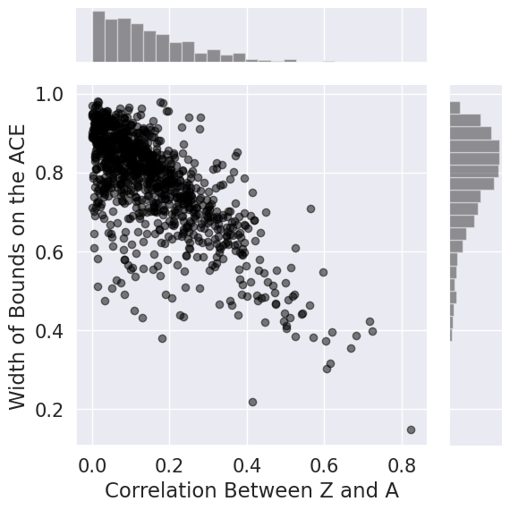
Figure 5: Each point represents a randomly generated distribution in the IV model with covariates, depicted in Fig. 3 (a). This plot shows informally that correlation between the generalized instrument $Z$ and the treatment $A$ is associated with tighter bounds on the ACE, $E[Y(A=1)-Y(A=0)]$. The histograms show the marginal distributions of correlation and bound width.

We observe that, as expected, greater correlation between the generalized instrument and the treatment is associated with tighter bounds. This pattern persisted across simulations for additional models, and across various approaches to sampling distributions from the model.

The marginal distributions of correlation and bound width, shown as histograms in Fig. 5 seem to be sensitive to the approach used to sample distributions from the model. For distributions sampled as described above, and used to generate Fig. 5, the mean width of bounds on the ACE was $0.77$, with a standard deviation of $0.12$. In $4\%$ of the distributions, the bounds excluded $0$. We find that these values are also sensitive to changes in how distributions were sampled.

Appendix E Bounds on $P(Y(\bar{a})=\bar{y})$ in the IV Model With Covariates

The remainder of this section is a LaTeX friendly printout of the steps taken by our implementation of the algorithm described in this work when applied to bounding $P(\bar{y}(\bar{a}))$ in the IV model with covariates, as described in Section 6.

To begin, we partition $\bar{y}(\bar{a})$ as described in Proposition 5:

$$\bar{y}(\bar{a})\land a(\bar{z})\land a(z)$$

$$\bar{a}(\bar{z})\land\bar{y}(\bar{z})$$

$$(a(\bar{z})\land(\bar{a}(z)\land\bar{y}(z))).$$

As before, no lower bound is provided for the first event in the partition, and the second has an identified density. We now consider the last event in the partition $a(\bar{z})\land(\bar{a}(z)\land\bar{y}(z))$.

The following events imply $a(\bar{z})$ and can therefore be used as $E_{1}$ events in Corollary 3:

$$a(\bar{z})\land\bar{y}(\bar{z})$$

$$a(\bar{z})\land y(\bar{z})$$

$$a(\bar{z})\land\bar{c}(\bar{z})$$

$$a(\bar{z})\land c(\bar{z})$$

$$a(\bar{z})\land\bar{y}(\bar{z})\land\bar{c}(\bar{z})$$

$$a(\bar{z})\land\bar{y}(\bar{z})\land c(\bar{z})$$

$$a(\bar{z})\land y(\bar{z})\land\bar{c}(\bar{z})$$

$$a(\bar{z})\land y(\bar{z})\land c(\bar{z}).$$

Likewise, the following events imply $\bar{a}(z)\land\bar{y}(z)$ and can therefore be used as $E_{2}$ events in Corollary 3:

$$\bar{a}(z)\land\bar{y}(z)$$

$$\bar{a}(z)\land\bar{y}(z)\land\bar{c}(z)$$

$$\bar{a}(z)\land\bar{y}(z)\land c(z)$$

By Proposition 10, $a(\bar{z})$, which implies $a(\bar{z})$, and therefore would be a candidate for use as an $E_{1}$ event, is redundant.

We now iterate through each potential event for $E_{1}$and $E_{2}$, examining the resulting bound.

The event $a(\bar{z})\land\bar{y}(\bar{z})$ is compatible with $\bar{y}(z)\lor(\bar{a}(z)\land y(z))$. Therefore to compute the bound induced by using it as an $E_{1}$ event, we must subtract from its density the portion of this compatible event that does not entail the negation of $\bar{a}(z)\land\bar{y}(z)$. This portion is $(a(z)\land\bar{y}(z))\lor(\bar{a}(z)\land y(z))$, yielding the bound $P_{\bar{z}}(a,\bar{y})-\big{(}P_{z}(a,\bar{y})+P_{z}(\bar{a},y)\big{)}$.

The event $a(\bar{z})\land y(\bar{z})$ is compatible with $(\bar{a}(z)\land\bar{y}(z))\lor y(z)$. Therefore to compute the bound induced by using it as an $E_{1}$ event, we must subtract from its density the portion of this compatible event that does not entail the negation of $\bar{a}(z)\land\bar{y}(z)$. This portion is $y(z)$, yielding the bound $P_{\bar{z}}(a,y)-P_{z}(y)$.

The event $a(\bar{z})\land\bar{c}(\bar{z})$ is compatible with $(a(z)\land\bar{c}(z))\lor c(z)$. Therefore to compute the bound induced by using it as an $E_{1}$ event, we must subtract from its density the portion of this compatible event that does not entail the negation of $\bar{a}(z)\land\bar{y}(z)$. This portion is $(a(z)\land y(z)\land\bar{c}(z))\lor(a(z)\land\bar{y}(z))\lor(y(z)\land c(z))$, yielding the bound $P_{\bar{z}}(a,\bar{c})-\big{(}P_{z}(a,y,\bar{c})+P_{z}(a,\bar{y})+P_{z}(y,c)\big{)}$.

The event $a(\bar{z})\land c(\bar{z})$ is compatible with $\bar{c}(z)\lor(a(z)\land c(z))$. Therefore to compute the bound induced by using it as an $E_{1}$ event, we must subtract from its density the portion of this compatible event that does not entail the negation of $\bar{a}(z)\land\bar{y}(z)$. This portion is $(y(z)\land\bar{c}(z))\lor(a(z)\land\bar{y}(z)\land\bar{c}(z))\lor(a(z)\land c(z))$, yielding the bound $P_{\bar{z}}(a,c)-\big{(}P_{z}(y,\bar{c})+P_{z}(a,\bar{y},\bar{c})+P_{z}(a,c)\big{)}$.

The event $a(\bar{z})\land\bar{y}(\bar{z})\land\bar{c}(\bar{z})$ is compatible with $(\bar{a}(z)\land y(z)\land c(z))\lor(a(z)\land\bar{y}(z)\land\bar{c}(z))\lor(\bar{y}(z)\land c(z))$. Therefore to compute the bound induced by using it as an $E_{1}$ event, we must subtract from its density the portion of this compatible event that does not entail the negation of $\bar{a}(z)\land\bar{y}(z)$. This portion is $(\bar{a}(z)\land y(z)\land c(z))\lor(a(z)\land\bar{y}(z))$, yielding the bound $P_{\bar{z}}(a,\bar{y},\bar{c})-\big{(}P_{z}(\bar{a},y,c)+P_{z}(a,\bar{y})\big{)}$.

The event $a(\bar{z})\land\bar{y}(\bar{z})\land c(\bar{z})$ is compatible with $(\bar{y}(z)\land\bar{c}(z))\lor(\bar{a}(z)\land y(z)\land\bar{c}(z))\lor(a(z)\land\bar{y}(z)\land c(z))$. Therefore to compute the bound induced by using it as an $E_{1}$ event, we must subtract from its density the portion of this compatible event that does not entail the negation of $\bar{a}(z)\land\bar{y}(z)$. This portion is $(\bar{a}(z)\land y(z)\land\bar{c}(z))\lor(a(z)\land\bar{y}(z))$, yielding the bound $P_{\bar{z}}(a,\bar{y},c)-\big{(}P_{z}(\bar{a},y,\bar{c})+P_{z}(a,\bar{y})\big{)}$.

The event $a(\bar{z})\land y(\bar{z})\land\bar{c}(\bar{z})$ is compatible with $(a(z)\land y(z)\land\bar{c}(z))\lor(\bar{a}(z)\land\bar{y}(z)\land c(z))\lor(y(z)\land c(z))$. Therefore to compute the bound induced by using it as an $E_{1}$ event, we must subtract from its density the portion of this compatible event that does not entail the negation of $\bar{a}(z)\land\bar{y}(z)$. This portion is $(a(z)\land y(z)\land\bar{c}(z))\lor(y(z)\land c(z))$, yielding the bound $P_{\bar{z}}(a,y,\bar{c})-\big{(}P_{z}(a,y,\bar{c})+P_{z}(y,c)\big{)}$.

The event $a(\bar{z})\land y(\bar{z})\land c(\bar{z})$ is compatible with $(y(z)\land\bar{c}(z))\lor(\bar{a}(z)\land\bar{y}(z)\land\bar{c}(z))\lor(a(z)\land y(z)\land c(z))$. Therefore to compute the bound induced by using it as an $E_{1}$ event, we must subtract from its density the portion of this compatible event that does not entail the negation of $\bar{a}(z)\land\bar{y}(z)$. This portion is $(y(z)\land\bar{c}(z))\lor(a(z)\land y(z)\land c(z))$, yielding the bound $P_{\bar{z}}(a,y,c)-\big{(}P_{z}(y,\bar{c})+P_{z}(a,y,c)\big{)}$.

The event $\bar{a}(z)\land\bar{y}(z)$is compatible with $\bar{y}(\bar{z})\lor(a(\bar{z})\land y(\bar{z}))$. Therefore to compute the bound induced by using it as an $E_{2}$ event, we must subtract from its density the portion of this compatible event that does not entail the negation of $a(\bar{z})$. This portion is $(\bar{a}(\bar{z})\land\bar{y}(\bar{z}))$, yielding the bound $P_{z}(\bar{a},\bar{y})-P_{\bar{z}}(\bar{a},\bar{y})$.

The event $\bar{a}(z)\land\bar{y}(z)\land\bar{c}(z)$is compatible with $(\bar{y}(\bar{z})\land c(\bar{z}))\lor(a(\bar{z})\land y(\bar{z})\land c(\bar{z}))\lor(\bar{a}(\bar{z})\land\bar{y}(\bar{z})\land\bar{c}(\bar{z}))$. Therefore to compute the bound induced by using it as an $E_{2}$ event, we must subtract from its density the portion of this compatible event that does not entail the negation of $a(\bar{z})$. This portion is $(\bar{a}(\bar{z})\land\bar{y}(\bar{z}))$, yielding the bound $P_{z}(\bar{a},\bar{y},\bar{c})-P_{\bar{z}}(\bar{a},\bar{y})$.

The event $\bar{a}(z)\land\bar{y}(z)\land c(z)$is compatible with $(\bar{a}(\bar{z})\land\bar{y}(\bar{z})\land c(\bar{z}))\lor(a(\bar{z})\land y(\bar{z})\land\bar{c}(\bar{z}))\lor(\bar{y}(\bar{z})\land\bar{c}(\bar{z}))$. Therefore to compute the bound induced by using it as an $E_{2}$ event, we must subtract from its density the portion of this compatible event that does not entail the negation of $a(\bar{z})$. This portion is $(\bar{a}(\bar{z})\land\bar{y}(\bar{z}))$, yielding the bound $P_{z}(\bar{a},\bar{y},c)-P_{\bar{z}}(\bar{a},\bar{y})$.

This concludes the derivation of the bounds presented for the IV model with covariates in Section 6.

References

- [1] Alexander Balke and Judea Pearl. Bounds on treatment effects from studies with imperfect compliance. Journal of the American Statistical Association, 92(439):1171–1176, 1997.
- [2] Alexander Abraham Balke. Probabilistic Counterfactuals: Semantics, Computation, and Applications. PhD thesis, USA, 1996.
- [3] Blai Bonet. Instrumentality tests revisited. In Proceedings of the Seventeenth Conference on Uncertainty and Artificial Intelligence, pages 48–55, 2001.
- [4] Robin J. Evans. Graphical methods for inequality constraints in marginalized dags. In Proceedings of the 2012 IEEE International Workshop on Machine Learning for Signal Processing, 2012.
- [5] Constantine Frangakis and Donald B. Rubin. Principal stratification in causal inference. Biometrics, 58(1):21–29, 2002.
- [6] Yimin Huang and Marco Valtorta. Pearl’s calculus of interventions is complete. In Twenty Second Conference On Uncertainty in Artificial Intelligence, 2006.
- [7] Changsung Kang and Jin Tian. Inequality constraints in causal models with hidden variables. In Proceedings of the Twenty Second Conference on Uncertainty in Artificial Intelligence, pages 233–240. AUAI Press, 2006.
- [8] Daniel Malinsky, Ilya Shpitser, and Thomas Richardson. A potential outcomes calculus for identifying conditional path-specific effects. Proceedings of machine learning research, 89:3080, 2019.
- [9] C.F. Manski. Nonparametric bounds on treatment effects. The American Economic Review, 80:319–323, 1990.
- [10] Jerzy Neyman. Sur les applications de la thar des probabilities aux experiences agaricales: Essay des principle. excerpts reprinted (1990) in English. Statistical Science, 5:463–472, 1923.
- [11] Judea Pearl. Causal inference from indirect experiments. Artificial intelligence in medicine, 7(6):561–582, 1995.
- [12] Judea Pearl. Causality: Models, Reasoning, and Inference. Cambridge University Press, 2 edition, 2009.
- [13] Roland R. Ramsahai. Causal bounds and observable constraints for non-deterministic models. Journal of Machine Learning Research, 2012.
- [14] Thomas S. Richardson, Robin J. Evans, James M. Robins, and Ilya Shpitser. Nested Markov properties for acyclic directed mixed graphs, 2017. Working paper.
- [15] Thomas S. Richardson and Jamie M. Robins. Single world intervention graphs (SWIGs): A unification of the counterfactual and graphical approaches to causality. preprint: http://www.csss.washington.edu/Papers/wp128.pdf, 2013.
- [16] James M. Robins. A new approach to causal inference in mortality studies with sustained exposure periods – application to control of the healthy worker survivor effect. Mathematical Modeling, 7:1393–1512, 1986.
- [17] James M. Robins. The analysis of randomized and non-randomized aids treatment trials using a new approach to causal inference in longitudinal studies. In L. Sechrest, H. Freeman, and A. Mulley, editors, Health Service Research Methodology: A Focus on AIDS, pages 113–159. NCHSR, U.S. Public Health Service, 1989.
- [18] Ilya Shpitser and Judea Pearl. Identification of joint interventional distributions in recursive semi-Markovian causal models. In Proceedings of the Twenty-First National Conference on Artificial Intelligence (AAAI-06). AAAI Press, Palo Alto, 2006.
- [19] Peter Spirtes, Clark Glymour, and Richard Scheines. Causation, Prediction, and Search. Springer Verlag, New York, 2 edition, 2001.
- [20] Jin Tian and Judea Pearl. On the testable implications of causal models with hidden variables. In Proceedings of the Eighteenth Conference on Uncertainty in Artificial Intelligence (UAI-02), volume 18, pages 519–527. AUAI Press, Corvallis, Oregon, 2002.
- [21] Thomas S. Verma and Judea Pearl. Equivalence and synthesis of causal models. Technical Report R-150, Department of Computer Science, University of California, Los Angeles, 1990.
- [22] Elie Wolfe, Robert AW. Spekkens, and Tobias Fritz. The inflation technique for causal inference with latent variables. https://arxiv.org/abs/1609.00672, 2016.