Nonlocal strain gradient exact solutions for functionally graded inflected nano-beams

Abstract

The size-dependent bending behavior of nano-beams is investigated by the modified nonlocal strain gradient elasticity theory. According to this model, the bending moment is expressed by integral convolutions of elastic flexural curvature and of its derivative with a bi-exponential averaging kernel. It has been recently proven that such a relation is equivalent to a differential equation, involving bending moment and flexural curvature fields, equipped with natural higher-order boundary conditions of constitutive type. The associated elastostatic problem of a Bernoulli-Euler functionally graded nanobeam is formulated and solved for simple statical schemes of technical interest. An effective analytical approach is presented and exploited to establish exact expressions of nonlocal strain gradient transverse displacements of doubly clamped, cantilever, clamped-pinned and pinned-pinned nano-beams, detecting thus also new benchmarks for numerical analyses. Comparisons with results of literature, corresponding to selected higher-order boundary conditions are provided and discussed. The considered nonlocal strain gradient model can be advantageously adopted to characterize scale phenomena in nano-engineering problems.

Keywords: Integral elasticity, Modified nonlocal strain gradient theory, Constitutive boundary conditions, Higher-order boundary conditions, Size effects, Nanobeams.

1 Introduction

In recent years new and multifunctional materials have been introduced requiring the consideration of small length scales [1, 2]. From an engineering standpoint, the realization of nano-actuators, nano-sensors, 3D printings and structural components for micro- and nano-systems has become an important topic, see e.g. the review papers [3, 4] and the contributions [5]-[16]. Since mechanical properties are size-dependent at the nanoscale, the study of size effects on the behaviour of nano-beams is an important area of research. It is well-known that the classical continuum theory neglects structural phenomena that are important at small-scales [17]-[30]. Accordingly new non-classical continuum theories can be adopted to model the size-dependency of micro- and nano-scale structures such as strain-driven and stress-driven nonlocal elasticity [31]-[34]. The strain-driven nonlocal elastic model has been introduced by Eringen [35] and the nonlocal stress is obtained in terms of the integral convolution of the elastic strain with a smoothing kernel. Such a model cannot be adopted to assess size-effects in nanomechanics, as proved in [36] and agreeded in several papers such as [37, 38]. Actually, the ill-posedness of Eringen’s strain-driven purely nonlocal elastic model for bounded domains relies on the fact that the constitutive boundary conditions associated with Eringen’s integral law conflict with equilibrium requirements, see [39, 40]. The stress-driven nonlocal elastic model for nano-beams has been provided in [41] and the nonlocal elastic strain is obtained in terms of the integral convolution of the stress with a smoothing kernel. This model leads to well-posed nonlocal problems for structures defined on bounded domains, see e.g. [42]-[45]. A recent approach proposed in [46] merges Eringen’s nonlocal strain-driven integral law with the strain gradient elasticity to obtain a higher-order nonlocal theory. The nonlocal stress is defined as the sum of two integral terms: the former is Eringen’s convolution between the elastic strain and a smoothing kernel depending on a nonlocal parameter and the latter is the derivative of the convolution of the elastic strain gradient with a smoothing kernel depending on a nonlocal parameter. If the bi-exponential function is considered for the smoothing kernel, the solution of the nonlocal problem is achieved, in literature, by replacing the integral law with the differential law which is considered to be equivalent to the integral relation. The main problem is that such a differential equation is of higher-order than the one of the classical local problem. As a consequence, additional (so-called) higher-order boundary conditions have to be imposed to solve the nonlocal strain gradient elastostatic problem. In literature, two different choices are provided consisting in imposing higher-order kinematic [47] or static [48] boundary conditions pertaining to the strain gradient theory. It is worth noting that the nonlocal structural response is particularly affected by these choices. A definitive answer to the discussion on the higher-order boundary conditions to be imposed in order to solve the elastostatic problem of nonlocal strain gradient nano-beams has been provided in [49]. It is proved that such boundary conditions follow from the nonlocal strain gradient integral law and turns out to be of constitutive kind. It is also shown in [49] that the differential problem, equipped with the correct constitutive boundary conditions, leads to well-posed elastostatic problems for bounded nano-structures. The nonlocal strain gradient elastic model is utilized in the present paper to address the size-dependent static behavior of inflected nano-beams of technical interest. Small-scale effects are exhibited by nano-beams for any boundary condition. In particular, closed form solutions for the nonlocal strain gradient model are given for cantilever, simply-supported, clamped-pinned and fully-clamped FG nano-beams subject to a uniform load. It is shown that nano-beams exhibit softening and stiffening structural behaviors for increasing nonlocal and gradient parameters respectively, so that the nonlocal strain gradient law provides an effective approach to design a wide class of nanodevices. If the gradient parameter vanishes, the constitutive boundary conditions of the nonlocal strain gradient law coincide to the ones of Eringen’s nonlocal integral law given in [36]. Numerical analyses are provided as benchmarks for applications and experiments involving inflected nano-beams.

2 Nonlocal strain gradient model for Bernoulli-Euler nano-beams

Nonlocal strain gradient (NSG) model of elasticity for inflected nano-beams, according to the model proposed in [46], is formulated by expressing the bending moment $M$ in terms of elastic flexural curvature $\chi_{el}$ and of its derivative $\partial_{x}\chi_{el}$ as

$$\begin{array}[]{l}M\left(x,\lambda_{0},\lambda_{1},l\right)=\left(\alpha_{0}\ast\left(K\cdot\chi_{el}\right)\right)\left(x,\lambda_{0}\right)-l^{2}\partial_{x}\left(\alpha_{1}\ast\left(K\cdot\partial_{x}\chi_{el}\right)\right)\left(x,\lambda_{1}\right)\\ \vspace{-4pt}\cr=\mathop{\displaystyle\int}_{0}^{L}\alpha_{0}\left(x-y,\lambda_{0}\right)\cdot\left(K\cdot\chi_{el}\right)\left(y\right)dy-l^{2}\partial_{x}\mathop{\displaystyle\int}_{0}^{L}\alpha_{1}\left(x-y,\lambda_{1}\right)\cdot\left(K\cdot\partial_{x}\chi_{el}\right)\left(y\right)dy.\end{array}$$ (1)

We consider a straight beams of length $L$, the $x$-coordinate is taken along the length of the nano-beam with the $y$-coordinate along the thickness and the $z$-coordinate along the width of the nano-beam.

The local elastic bending stiffness is $K=I_{E}$ where $I_{E}=\int_{\Omega}E\left(y\right)dA$ is the second moment of the field of Young elastic moduli $E$ along the $y$ bending axis. The smoothing kernels $\alpha_{0}$ and $\alpha_{1}$ depend on two non-dimensional non-local parameters $\lambda_{0}$ $>$ 0 and $\lambda_{1}$ $>$ 0 . The characteristic length $l\geq 0$ has been introduced to make dimensionally homogeneous the convolutions in Eq. (1). Following [46] - [47], we consider that the nonlocal parameters are coincident, i.e. $\lambda$ $:=\lambda_{0}$ $=\lambda_{1}$, and the kernels $\alpha_{0}$ and $\alpha_{1}$ are coincident with the bi-exponential averaging function given by

$$\phi(x,c)=\dfrac{1}{2c}\exp\left(-\dfrac{\left|x\right|}{c}\right),$$ (2)

being $c=\lambda L$ the characteristic length of Eringen nonlocal elasticity. The bi-exponential function fulfils positivity, symmetry, normalisation and impulsivity, Introducing the following fields [46]

$$\begin{array}[]{l}M_{0}\left(x,c\right)=\mathop{\displaystyle\int}_{0}^{L}\phi\left(x-y,c\right)\cdot\left(K\cdot\chi_{el}\right)\left(y\right)dy\\ \vspace{-4pt}\cr M_{1}\left(x,c,l\right)=l^{2}\partial_{x}\mathop{\displaystyle\int}_{0}^{L}\phi\left(x-y,c\right)\cdot\left(K\cdot\partial_{x}\chi_{el}\right)\left(y\right)dy,\end{array}$$ (3)

the nonlocal strain gradient elastic law Eq. (1) can then be rewritten as

$$M\left(x,c,l\right)=M_{0}\left(x,c\right)-\partial_{x}M_{1}\left(x,c,l\right).$$ (4)

Since the bi-exponential averaging kernel Eq. (2) is the Green function on the whole real axis of Helmholtz linear differential operator $\mathcal{L}_{c}=1-c^{2}\partial_{x}^{2}$, the differential constitutive relation ensuing the nonlocal strain gradient law Eq. (4) can be written as

$$\left(K\cdot\chi_{el}\right)\left(x\right)-l^{2}\partial_{x}^{2}\left(K\cdot\chi_{el}\right)\left(x\right)=M\left(x,c,l\right)-c^{2}\ \partial_{x}^{2}M\left(x,c,l\right).$$ (5)

It is proved in [49] that the nonlocal strain gradient integral relation Eq. (4) is not equivalent to the differential law Eq. (5) for nano-beams defined on a bounded interval $[0,L]$. In fact suitable boundary conditions must be prescribed to ensure the constitutive equivalence according to the following proposition proved for the first time in [49]. Proposition 1 - Constitutive equivalence property. The nonlocal strain gradient constitutive law Eq. (4) equipped with the bi-exponential kernel Eq. (2)

$$M\left(x,c,l\right)=M_{0}\left(x,c\right)-\partial_{x}M_{1}\left(x,c,l\right),$$ (6)

with $x\in\left[0,L\right]$, is equivalent to the differential relation Eq. (5)

$$\left(K\cdot\chi_{el}\right)\left(x\right)-l^{2}\partial_{x}^{2}\left(K\cdot\chi_{el}\right)\left(x\right)=M\left(x,c,l\right)-c^{2}\ \partial_{x}^{2}M\left(x,c,l\right)$$ (7)

subject to the following two constitutive boundary conditions (CBC)

$$\left\{\begin{array}[]{l}\begin{array}[]{l}\partial_{x}M\left(0,c,l\right)=\dfrac{1}{c}M\left(0,c,l\right)+\dfrac{l^{2}}{c^{2}}\partial_{x}\left(K\cdot\chi_{el}\right)\left(a\right)\\ \vspace{-4pt}\cr\partial_{x}M\left(L,c,l\right)=-\dfrac{1}{c}M\left(L,c,l\right)+\dfrac{l^{2}}{c^{2}}\partial_{x}\left(K\cdot\chi_{el}\right)\left(L\right).\end{array}\end{array}\right.$$ (8)

$\hfill\blacksquare$

3 Static flexural analysis

To demonstrate the differences in the flexural results of the proposed nonlocal model and the existing models in the literature, a flexural beam problem with the Bernoulli-Euler kinematics is investigated. The well-established differential and classical boundary conditions of static equilibrium may be expressed as

$$\begin{array}[]{l}{\partial_{x}^{2}M\left(x\right)=q}\\ {\left.M\left(\partial_{x}\delta v\right)\right|_{0,L}=\left.\left(\partial_{x}M\right)\delta v\right|_{0,L}=0.}\end{array}$$ (9)

Assuming coincidence of elastic and total flexural curvatures $\,\chi_{el}=\chi\,$ and employing the differential equation of equilibrium in addition to the condition of kinematic compatibility $\,\chi=\partial_{x}^{2}v\,$, the bending moment introduced in Eq. (7) can be expressed as

$$M\left(x\right)=c^{2}q+\left(K\cdot\partial_{x}^{2}v\right)\left(x\right)-l^{2}\partial_{x}^{2}\left(K\cdot\partial_{x}^{2}v\right)\left(x\right)$$ (10)

In terms of deflection of nano-beam, the differential governing equation takes the form

$$\partial_{x}^{2}\left(K\cdot\partial_{x}^{2}v\right)\left(x\right)-l^{2}\partial_{x}^{4}\left(K\cdot\partial_{x}^{2}v\right)\left(x\right)=q-c^{2}\cdot\partial_{x}^{2}q$$ (11)

equipped with the classical boundary conditions Eq. (9)₂ and the constitutive boundary conditions Eq. (8). Employing the proposed nonlocal model, the exact solutions of the flexural analysis are derived for nano-beams with customary boundary conditions and subject to distributed loads. For a uniformly distributed load $q_{0}$, analytical solution of the static equations governing the flexural deflection of the nano-beam, Eq. (11), can be expressed by

$$v\left(x\right)=\frac{q_{0}x^{4}}{24K}+\Gamma_{1}\mathrm{exp}\left(\frac{x}{l}\right)l^{4}+\Gamma_{2}\mathrm{exp}\left(-\frac{x}{l}\right)l^{4}+\Gamma_{3}x^{3}+\Gamma_{4}x^{2}+\Gamma_{5}x+\Gamma_{6}$$ (12)

where $\Gamma_{k}\left(k=1,\ldots,6\right)$ are unknown constants to be determined by suitable boundary conditions including the well-known classical boundary conditions Eq. (9)₂ and the constitutive boundary conditions Eq. (8). The exact analytical solutions for flexure problem of Bernoulli-Euler nano-beams will be also compared with the counterpart results introduced in the literature by prescribing different kind of higher-order constitutive boundary conditions. Assuming coincidence of elastic and total flexural curvatures $\,\chi_{el}=\chi\,$, the higher-order constitutive boundary conditions adopted in literature may be expressed as either of the following conditions [47]. The first constitutive boundary conditions, referred to as Kinematic Higher-Order Boundary Conditions (KHOBC), are expressed by the vanishing of the flexural curvature at the end cross-sections

$$\left.\chi\right|_{x=0,L}=\left.\partial_{x}^{2}v\right|_{x=0,L}=0$$ (13)

The second constitutive boundary conditions, referred to as Static Higher-Order Boundary Conditions (SHOBC), are expressed by the vanishing of the derivative of flexural curvature at the end cross-sections

$$\left.\partial_{x}\chi\right|_{x=0,L}=\left.\partial_{x}^{3}v\right|_{x=0,L}=0$$ (14)

Bernoulli-Euler nano-beam with four different sets of boundary conditions including doubly clamped, clamped-simply supported, simply supported and cantilever nano-beams under a uniform load $q_{0}$ are examined.

While the set of classical boundary conditions are enforced to the beam ends according to local Bernoulli-Euler beam theory, the constitutive boundary conditions are imposed to corresponding beam ends in the proposed nonlocal model as Eq. (8) yielding in the deflection v and the higher-order constitutive boundary conditions as Eq. (13) and (14) are enforced for the counterpart models resulting in the deflections $v^{\mathrm{KHOBC}}$and $v^{\mathrm{SHOBC}}$, respectively. Also, the acronyms CC, CF, CS and SS stand for doubly clamped, clamped-free, clamped-simply supported and simply supported boundary conditions, respectively. The following non-dimensional variable $\zeta$, the non-dimensional characteristic parameters $\lambda$ and $\mu$ as well as the non-dimensional deflection $\bar{v}$ are also employed for the examples

$$\zeta=\frac{x}{L},\mathrm{\;\;\;\;\;\;}\lambda=\frac{c}{L},\mathrm{\;\;\;\;\;\;}\mu=\frac{l}{L},\mathrm{\;\;\;\;\;\;}\bar{v}=v\frac{K}{q_{0}L^{4}}$$ (15)

3.1 Doubly clamped nano-beam

A doubly clamped nano-beam of length L under a uniform load $q_{0}$ is first considered. The classical boundary conditions for doubly clamped nano-beam are given by,

$$\begin{array}[]{l}{v\left(0\right)=\partial_{x}v\left(0\right)=0}\\ {v\left(L\right)=\partial_{x}v\left(L\right)=0}\end{array}$$ (16)

Employing the set of classical and higher-order boundary conditions to the flexural deflection of the nano-beam Eq. (12), the transverse displacement field $\bar{v}$ and $\bar{v}^{\mathrm{KHOBC}},\bar{v}^{\mathrm{SHOBC}}$according to the nonlocal model and the counterpart theories can be determined as

$$\begin{array}[]{l}{\bar{v}\left(\zeta\right)=\frac{1}{24}\left(-2\zeta^{3}+\zeta^{4}-\frac{\zeta^{2}\left(-1+12\lambda^{2}+24\lambda^{3}-12\mu^{2}-24\lambda\mu^{2}\right)}{1+2\lambda}+\frac{2\zeta\left(\lambda+6\lambda^{2}+12\lambda^{3}-6\mu^{2}-12\lambda\mu^{2}\right)}{1+2\lambda}\right.}\\ \vspace{-4pt}\cr{\mathrm{\;\;\;\;\;\;\;\;}\left.-2\frac{\left(\mathrm{e}^{\frac{1-\zeta}{\mu}}+\mathrm{e}^{\zeta/\mu}-\left(1+\mathrm{e}^{1/\mu}\right)\right)\mu\left(-6\lambda^{2}-12\lambda^{3}+6\mu^{2}+\lambda\left(-1+12\mu^{2}\right)\right)}{\left(-1+\mathrm{e}^{1/\mu}\right)\left(1+2\lambda\right)}\right)}\\ \vspace{-4pt}\cr{\bar{v}^{\mathrm{KHOBC}}\left(\zeta\right)=\frac{\mathrm{e}^{-\frac{\zeta}{\mu}}}{24\left(-1-2\mu+\mathrm{e}^{1/\mu}\left(-1+2\mu\right)\right)}\left(2\left(\mathrm{e}^{1/\mu}+\mathrm{e}^{2\zeta/\mu}\right)\mu^{2}-\mathrm{e}^{\zeta/\mu}\left(\zeta^{2}+2\zeta\mu+2\mu^{2}\right.\right.}\\ \vspace{-4pt}\cr{\mathrm{\;\;\;\;\;\;\;\;\;\;\;\;\;\;\;}\left.\left.-\left(2\zeta^{3}-\zeta^{4}\right)\left(1+2\mu\right)\right)-\mathrm{e}^{\frac{1+\zeta}{\mu}}\left(\zeta^{2}+\left(\zeta^{4}-2\zeta^{3}\right)\left(1-2\mu\right)-2\zeta\mu+2\mu^{2}\right)\right)}\\ \vspace{-4pt}\cr{\bar{v}^{\mathrm{SHOBC}}\left(\zeta\right)=\frac{\mathrm{e}^{-\frac{\zeta}{\mu}}}{24\left(-1+\mathrm{e}^{1/\mu}\right)}\left(-12\mu^{3}\left(\mathrm{e}^{1/\mu}+\mathrm{e}^{2\zeta/\mu}\right)-\mathrm{e}^{\zeta/\mu}\left(-2\zeta^{3}+\zeta^{4}-12\zeta\mu^{2}-12\mu^{3}\right.\right.}\\ \vspace{-4pt}\cr{\left.\left.\mathrm{\;\;\;\;\;\;\;\;\;\;\;\;\;\;}+\zeta^{2}\left(1+12\mu^{2}\right)\right)+\mathrm{e}^{\frac{1+\zeta}{\mu}}\left(-2\zeta^{3}+\zeta^{4}-12\zeta\mu^{2}+12\mu^{3}+\zeta^{2}\left(1+12\mu^{2}\right)\right)\right)}\end{array}$$ (17)

The maximum deflection of the doubly clamped nano-beam is attained at the mid-span as

$$\begin{array}[]{l}{\bar{v}_{\max}=\frac{\left(1+10\lambda+48\lambda^{2}+96\lambda^{3}-48\left(1+2\lambda\right)\mu^{2}-32\mu\tanh\left(\frac{1}{4\mu}\right)\left(\lambda\left(1+6\lambda\left(1+2\lambda\right)\right)-6\left(1+2\lambda\right)\mu^{2}\right)\right)}{384\left(1+2\lambda\right)}}\\[6.45831pt] {\bar{v}_{\max}^{\mathrm{KHOBC}}=\frac{-1+64\mathrm{e}^{\frac{1}{2\mu}}\mu^{2}-2\mu\left(5+16\mu\right)+\mathrm{e}^{1/\mu}\left(-1+2\left(5-16\mu\right)\mu\right)}{384\left(-1-2\mu+\mathrm{e}^{1/\mu}\left(-1+2\mu\right)\right)}}\\[8.61108pt] {\bar{v}_{\max}^{\mathrm{SHOBC}}=\frac{1}{384}-\frac{\mu^{2}}{8}+\frac{1}{2}\mu^{3}\tanh\left(\frac{1}{4\mu}\right)}\end{array}$$ (18)

It is apparent from Eq. (17) that the non-dimensional transverse displacements $\bar{v}^{\mathrm{KHOBC}}$ and $\bar{v}^{\mathrm{SHOBC}}$ are independent of non-dimensional characteristic parameter $\lambda$.

3.2 Nano-cantilever

A nano-cantilever with length L subject to a uniform load$q_{0}$can be dealt with in a similar way. The classical boundary conditions for clamped-simply supported nano-beam are written as

$$\begin{array}[]{l}{v\left(0\right)=\partial_{x}v\left(0\right)=0}\\ {M_{\lambda}\left(L\right)=\partial_{x}M_{\lambda}\left(L\right)=0}\end{array}$$ (19)

Utilizing the set of classical and higher-order boundary conditions in the flexural deflection of the nano-beam Eq. (12), the transverse displacement field $\bar{v}$and $\bar{v}^{\mathrm{KHOBC}},\bar{v}^{\mathrm{SHOBC}}$ in accordance with the nonlocal model and the counterpart theories can be determined as,

$$\begin{array}[]{l}{\bar{v}\left(\zeta\right)=\frac{1}{24}\left(-4\zeta^{3}+\zeta^{4}+12\zeta\left(\lambda+2\lambda^{2}-2\mu^{2}\right)+6\zeta^{2}\left(1-2\lambda^{2}+2\mu^{2}\right)\right.}\\ {\mathrm{\;\;\;\;\;\;\;\;}\left.-\frac{12\mu\left(-\lambda-2\lambda^{2}+2\mu^{2}\right)}{-1+\mathrm{e}^{2/\mu}}\left(\mathrm{e}^{\frac{2-\zeta}{\mu}}+\mathrm{e}^{\zeta/\mu}-\mathrm{e}^{2/\mu}-1\right)\right)}\\ {\bar{v}^{\mathrm{KHOBC}}\left(\zeta\right)=\frac{1}{24}(-4\zeta^{3}+\zeta^{4}+6\left(\zeta^{2}+2\mu^{2}\right)\left(1-2\lambda^{2}+2\mu^{2}\right)-\frac{12\mathrm{e}^{\frac{\zeta}{\mu}}\mu^{2}\left(-1-2\left(-1+\mathrm{e}^{1/\mu}\right)\left(\lambda^{2}-\mu^{2}\right)\right)}{-1+\mathrm{e}^{2/\mu}}}\\ {\mathrm{\;\;\;\;\;\;\;\;\;\;\;\;\;\;\;}\left.-\frac{12\zeta\mu\left(1+\mathrm{e}^{2/\mu}-2\left(-1+\mathrm{e}^{1/\mu}\right)^{2}\left(\lambda^{2}-\mu^{2}\right)\right)}{-1+\mathrm{e}^{2/\mu}}-\frac{12\mathrm{e}^{\frac{1-\zeta}{\mu}}\mu^{2}\left(2\left(\lambda^{2}-\mu^{2}\right)+\mathrm{e}^{1/\mu}\left(1-2\lambda^{2}+2\mu^{2}\right)\right)}{-1+\mathrm{e}^{2/\mu}}\right)}\\ {\bar{v}^{\mathrm{SHOBC}}\left(\zeta\right)=\frac{\mathrm{e}^{-\frac{\zeta}{\mu}}}{24(-1+\mathrm{e}^{2/\mu})}\left(-24\mu^{3}\left(\mathrm{e}^{2/\mu}+\mathrm{e}^{\frac{2\zeta}{\mu}}\right)\right.+\mathrm{e}^{\zeta/\mu}\left(4\zeta^{3}-\zeta^{4}+24\zeta\mu^{2}+24\mu^{3}+6\zeta^{2}\left(-1\right.\right.}\\ {\mathrm{\;\;\;\;\;\;\;\;\;\;\;\;\;\;\;}\left.\left.\left.+2\lambda^{2}-2\mu^{2}\right)\right)+\mathrm{e}^{\frac{2+\zeta}{\mu}}\left(-4\zeta^{3}+\zeta^{4}-24\zeta\mu^{2}+24\mu^{3}+\zeta^{2}\left(6-12\lambda^{2}+12\mu^{2}\right)\right)\right)}\end{array}$$ (20)

which depends on both non-dimensional characteristic parameters$\lambda$and $\mu$. Also, the maximum deflection of the nano-beam is attained at the tip as,

$$\begin{array}[]{l}{\bar{v}_{\max}=\frac{\mu\left(\lambda+2\lambda^{2}-2\mu^{2}\right)}{1+\mathrm{e}^{\frac{1}{\mu}}}+\frac{1}{8}\left(\left(1+2\lambda\right)^{2}-4\lambda\left(1+2\lambda\right)\mu-4\mu^{2}+8\mu^{3}\right)}\\ \vspace{-4pt}\cr{\bar{v}_{\max}^{\mathrm{KHOBC}}=-\frac{1}{8}\left(-2\mu+\coth\left(\frac{1}{2\mu}\right)\right)\left(\left(-1+4\lambda^{2}-4\mu^{2}\right)\tanh\left(\frac{1}{2\mu}\right)+2\mu\right)}\\ \vspace{-4pt}\cr{\bar{v}_{\max}^{\mathrm{SHOBC}}=\frac{1}{8}\left(1-4\lambda^{2}-4\mu^{2}+8\mu^{3}\tanh\left(\frac{1}{2\mu}\right)\right)}\end{array}$$ (21)

3.3 Clamped-simply supported nano-beam

To examine a clamped-simply supported nano-beam with length L subject to a uniform load $q_{0}$, the classical boundary conditions are considered as

$$\begin{array}[]{l}{v\left(0\right)=\partial_{x}v\left(0\right)=0}\\ {v\left(L\right)=M_{\lambda}\left(L\right)=0.}\end{array}$$ (22)

As a result of imposing the set of classical and higher-order boundary conditions to the flexural deflection of the nano-beam Eq. (12), the transverse displacement field $\bar{v}$ and $\bar{v}^{\mathrm{KHOBC}}$, $\bar{v}^{\mathrm{SHOBC}}$ consistent with the nonlocal model and the counterpart theories can be determined as

$$\begin{array}[]{l}{\bar{v}\left(\zeta\right)=\frac{-\mathrm{e}^{1/\mu}}{24\left(-1+\mathrm{e}^{1/\mu}\right)\left(1+3\lambda\left(1+\mu\right)-3\mu^{2}\left(1+2\mu\right)+\lambda^{2}\left(3+6\mu\right)+\mathrm{e}^{1/\mu}\left(1+3\lambda\left(1+\lambda\right)-3\lambda\left(1+2\lambda\right)\mu-3\mu^{2}+6\mu^{3}\right)\right)}}\\ {\mathrm{\;\;\;\;\;\;\;\;\;}\left(6\lambda\left(1+2\lambda\right)\left(-\left(-2+\zeta\right)\zeta^{3}+3\lambda+6\left(1+2\left(-1+\zeta\right)\zeta\right)\lambda^{2}\right)\mu\right.}\\ {\mathrm{\;\;\;\;\;\;\;\;\;}-6\left(3+4\zeta^{3}-2\zeta^{4}+12\left(1+\left(-1+\zeta\right)\zeta\right)\lambda+24\left(1+2\left(-1+\zeta\right)\zeta\right)\lambda^{2}\right)\mu^{3}}\\ {\mathrm{\;\;\;\;\;\;\;\;\;}+72\left(1+2\left(-1+\zeta\right)\zeta\right)\mu^{5}-6\mu\cosh\left(\frac{1}{\mu}\right)\left(-\lambda\left(1+2\lambda\right)\right.}\\ {\mathrm{\;\;\;\;\;\;\;\;\;}\left.\left(1-2\zeta^{3}+\zeta^{4}+3\lambda+6\left(1-2\left(-1+\zeta\right)\zeta\right)\lambda^{2}\right)\right.}\\ {\mathrm{\;\;\;\;\;\;\;\;\;}+\left(5+2\left(-2+\zeta\right)\zeta^{3}+12\lambda-12\left(-1+\zeta\right)\zeta\lambda+24\left(1-2\left(-1+\zeta\right)\zeta\right)\lambda^{2}\right)\mu^{2}}\\ {\left.\mathrm{\;\;\;\;\;\;\;\;\;}+12\left(-1+2\left(-1+\zeta\right)\zeta\right)\mu^{4}\right)-6\mu\cosh\left(\frac{1-\zeta}{\mu}\right)\left(\lambda\left(1+2\lambda\right)\right.}\\ {\mathrm{\;\;\;\;\;\;\;\;\;}\left.\left(1+3\lambda+6\lambda^{2}\right)-\left(5+12\lambda\left(1+2\lambda\right)\right)\mu^{2}+12\mu^{4}\right)+\zeta^{2}\left(-3+\left(5-2\zeta\right)\zeta\right)\sinh\left(\frac{1}{\mu}\right)}\\ {\mathrm{\;\;\;\;\;\;\;\;\;}-6\sinh\left(\frac{1}{\mu}\right)\left(\left(-1+\zeta\right)\zeta\lambda\left(-1-5\lambda+\left(1+\lambda\right)\left(\left(-1+\zeta\right)\zeta-12\lambda^{2}\right)\right)\right.}\\ {\mathrm{\;\;\;\;\;\;\;\;\;}+\mu^{2}\left(-\left(-1+\zeta\right)\zeta\left(-5+\left(-1+\zeta\right)\zeta\right)+12\left(-1+\zeta\right)\zeta\lambda+24\left(-1+\zeta\right)\zeta\lambda^{2}\right.}\\ {\left.\mathrm{\;\;\;\;\;\;\;\;\;}\left.+12\lambda^{3}+24\lambda^{4}\right)-12\left(\left(-1+\zeta\right)\zeta+\lambda+4\lambda^{2}\right)\mu^{4}+24\mu^{6}\right)}\\ {\mathrm{\;\;\;\;\;\;\;\;\;}+18\mu\left(-\lambda^{2}+\mu^{2}\right)\cosh\left(\frac{\zeta}{\mu}\right)\left(\left(1+2\lambda\right)^{2}-4\mu^{2}-4\mu\left(\lambda+2\lambda^{2}-2\mu^{2}\right)\sinh\left(\frac{1}{\mu}\right)\right)}\\ {\mathrm{\;\;\;\;\;\;\;\;\;}\left.-144\left(\lambda^{2}-\mu^{2}\right)\mu^{2}\left(\lambda+2\lambda^{2}-2\mu^{2}\right)\sinh\left(\frac{1}{2\mu}\right)^{2}\sinh\left(\frac{\zeta}{\mu}\right)\right)}\\[8.61108pt] {\bar{v}^{\mathrm{KHOBC}}\left(\zeta\right)=\frac{\mathrm{e}^{1/\mu}}{24\left(-1-3\mu\left(1+\mu\right)+\mathrm{e}^{2/\mu}\left(1+3\left(-1+\mu\right)\mu\right)\right)}}\\ {\mathrm{\;\;\;\;\;\;\;\;\;\;\;\;\;\;\;\;}\left(-24\left(-1+\zeta\right)\left(\lambda^{2}-\mu^{2}\right)\mu\left(\left(-2+\zeta\right)\zeta+6\mu^{2}\right)\right.}\\ {\mathrm{\;\;\;\;\;\;\;\;\;\;\;\;\;\;\;\;}-6\zeta\mu\cosh\left(\frac{1}{\mu}\right)\left(1+4\lambda^{2}+\zeta^{2}\left(-2+\zeta-4\lambda^{2}\right)+4\left(-1+\zeta^{2}-6\lambda^{2}\right)\mu^{2}+24\mu^{4}\right)}\\ {\mathrm{\;\;\;\;\;\;\;\;\;\;\;\;\;\;\;\;}+\sinh\left(\frac{1}{\mu}\right)\left(\left(-1+\zeta\right)\zeta^{2}\left(-3+2\zeta-12\lambda^{2}\right)+6\left(\left(-1+\zeta^{2}\right)^{2}+4\left(1-3\zeta^{2}\right)\lambda^{2}\right)\mu^{2}\right.}\\ {\left.\mathrm{\;\;\;\;\;\;\;\;\;\;\;\;\;\;\;\;}+24\left(-1+3\zeta^{2}-6\lambda^{2}\right)\mu^{4}+144\mu^{6}\right)+6\mu^{2}\cosh\left(\frac{\zeta}{\mu}\right)\left(24\mu\left(-\lambda^{2}+\mu^{2}\right)\right.}\\ {\left.\mathrm{\;\;\;\;\;\;\;\;\;\;\;\;\;\;\;\;}+\left(-1+4\mu^{2}-24\mu^{4}+4\lambda^{2}\left(-1+6\mu^{2}\right)\right)\sinh\left(\frac{1}{\mu}\right)\right)+6\mu^{2}\left(8\left(\lambda^{2}-\mu^{2}\right)\left(1+3\mu^{2}\right)\right.}\\ {\left.\mathrm{\;\;\;\;\;\;\;\;\;\;\;\;\;\;\;\;}\left.+\left(1+4\lambda^{2}-4\left(1+6\lambda^{2}\right)\mu^{2}+24\mu^{4}\right)\cosh\left(\frac{1}{\mu}\right)\right)\sinh\left(\frac{\zeta}{\mu}\right)\right)}\end{array}$$

$$\begin{array}[]{l}{\bar{v}^{\mathrm{SHOBC}}\left(\zeta\right)=\frac{\mathrm{e}^{-\frac{\zeta}{\mu}}}{48\left(-1+\mathrm{e}^{1/\mu}\right)\left(1-3\mu^{2}-6\mu^{3}+\mathrm{e}^{1/\mu}\left(1-3\mu^{2}+6\mu^{3}\right)\right)}}\\ {\mathrm{\;\;\;\;\;\;\;\;\;\;\;\;\;\;\;}\left(-18\mathrm{e}^{\frac{1+2\zeta}{\mu}}\mu^{3}\left(1-4\lambda^{2}-4\mu^{2}+8\mu^{3}\right)+18\mathrm{e}^{\frac{1}{\mu}}\mu^{3}\left(-1+4\lambda^{2}+4\mu^{2}+8\mu^{3}\right)\right.}\\ {\mathrm{\;\;\;\;\;\;\;\;\;\;\;\;\;\;\;}-6\mathrm{e}^{2/\mu}\mu^{3}\left(5+12\lambda^{2}-12\mu^{2}+24\mu^{3}\right)+6\mathrm{e}^{\frac{2\zeta}{\mu}}\mu^{3}\left(-5-12\lambda^{2}+12\mu^{2}+24\mu^{3}\right)}\\ {\mathrm{\;\;\;\;\;\;\;\;\;\;\;\;\;\;\;}-12\mathrm{e}^{\frac{1+\zeta}{\mu}}\mu^{3}\left(-4\zeta^{3}+2\zeta^{4}-24\zeta\mu^{2}-24\zeta^{2}\left(\lambda^{2}-\mu^{2}\right)+3\left(-1+4\lambda^{2}+4\mu^{2}\right)\right)}\\ {\mathrm{\;\;\;\;\;\;\;\;\;\;\;\;\;\;\;}+\mathrm{e}^{\frac{2+\zeta}{\mu}}\left(2\zeta^{4}\left(1-3\mu^{2}+6\mu^{3}\right)-\left(\zeta^{3}+6\zeta\mu^{2}+6\mu^{3}\right)\left(5+12\lambda^{2}-12\mu^{2}+24\mu^{3}\right)\right.}\\ {\left.\mathrm{\;\;\;\;\;\;\;\;\;\;\;\;\;\;\;}+3\zeta^{2}\left(1+8\mu^{2}-24\mu^{4}+48\mu^{5}+\lambda^{2}\left(4+24\mu^{2}-48\mu^{3}\right)\right)\right)}\\ {\mathrm{\;\;\;\;\;\;\;\;\;\;\;\;\;\;\;}\mathrm{+e}^{\zeta/\mu}\left(\left(\zeta^{3}+6\mu^{3}+6\zeta\mu^{2}\right)\left(5+12\lambda^{2}-12\mu^{2}-24\mu^{3}\right)\right.+2\zeta^{4}\left(-1+3\mu^{2}+6\mu^{3}\right)}\\ {\mathrm{\;\;\;\;\;\;\;\;\;\;\;\;\;\;}\left.\left.+3\zeta^{2}\left(1+8\mu^{2}-24\mu^{4}-48\mu^{5}+4\lambda^{2}\left(1+6\mu^{2}+12\mu^{3}\right)\right)\right)\right)}\end{array}$$ (23)

which also depends on both non-dimensional characteristic parameters $\lambda$ and $\mu$. The deflection of the nano-beam at the mid-span will be employed for the next figures

$$\begin{array}[]{l}{\tilde{v}=\frac{1}{384\left(1+\mathrm{e}^{\frac{1}{2\mu}}\right)}}\\ {\mathrm{\;\;\;}\frac{1}{\left(1+3\lambda\left(1+\mu\right)-3\left(\mu^{2}-\lambda^{2}\right)\left(1+2\mu\right)+\mathrm{e}^{1/\mu}\left(1+3\lambda\left(1+\lambda\right)-3\lambda\left(1+2\lambda\right)\mu-3\mu^{2}+6\mu^{3}\right)\right)}}\\ {\mathrm{\;\;\;}\left(\mathrm{2}+\mathrm{e}^{\frac{1}{2\mu}}\left(2+3\left(\lambda\left(5+3\lambda\left(7+16\lambda\left(1+\lambda\right)\right)\right)-3\lambda\left(1+2\lambda\right)\left(1+16\lambda\left(1+\lambda\right)\right)\mu\right.\right.\right.}\\ {\mathrm{\;\;\;}-3\left(7+16\lambda\left(1+2\lambda\right)\left(1+4\lambda^{2}\right)\right)\mu^{2}+6\left(9+8\lambda\left(3+4\lambda\right)\right)\mu^{3}}\\ {\mathrm{\;\;\;}\left.\left.+48\left(1+4\lambda\left(1+4\lambda\right)\right)\mu^{4}-96\mu^{5}-384\mu^{6}\right)\right)}\\ {\mathrm{\;\;\;}+\mathrm{e}^{1/\mu}\left(2+3\left(\lambda\left(5+3\lambda\left(7+16\lambda\left(1+\lambda\right)\right)\right)+3\lambda\left(1+2\lambda\right)\left(1+16\lambda\left(1+\lambda\right)\right)\mu\right.\right.}\\ {\mathrm{\;\;\;}-3\left(7+16\lambda\left(1+2\lambda\right)\left(1+4\lambda^{2}\right)\right)\mu^{2}-6\left(9+8\lambda\left(3+4\lambda\right)\right)\mu^{3}}\\ {\mathrm{\;\;\;}\left.\left.+48\left(1+4\lambda\left(1+4\lambda\right)\right)\mu^{4}+96\mu^{5}-384\mu^{6}\right)\right)}\\ {\mathrm{\;\;\;}+\mathrm{e}^{\frac{3}{2\mu}}\left(2+3\left(\lambda\left(5+3\lambda\left(7+16\lambda\left(1+\lambda\right)\right)\right)-\lambda\left(1+2\lambda\right)\left(13+48\lambda\left(1+3\lambda\right)\right)\mu\right.\right.}\\ {\mathrm{\;\;\;}+3\left(-7+16\lambda\left(-1+2\lambda\right)\left(1+2\lambda\right)^{2}\right)\mu^{2}-2\left(37+24\lambda\left(5+12\lambda\right)\right)\mu^{3}}\\ {\mathrm{\;\;\;}\left.\left.-48\left(-1+4\lambda\left(1+4\lambda\right)\right)\mu^{4}-288\mu^{5}+384\mu^{6}\right)\right)+3\left(48\lambda^{3}\left(1+\lambda\right)\left(1+4\lambda\right)\right.}\\ {\mathrm{\;\;\;}\left.+48\lambda^{4}\left(1+6\mu+8\mu^{2}\right)+\lambda\left(5-\mu\left(-13+48\mu\left(1+\mu\right)\left(1+4\mu\right)\right)+\mu^{2}\left(-21+2\mu\left(-37\right)\right.\right.\right.}\\ {\mathrm{\;\;\;}\left.\left.\left.\left.+24\mu\left(1+2\mu\right)\left(1+4\mu\right)\right)\right)+\lambda^{2}\left(21-2\mu\left(-37+48\mu\left(1+2\mu\right)\left(1+4\mu\right)\right)\right)\right)\right)}\end{array}$$

$$\begin{array}[]{l}{\tilde{v}^{\mathrm{KHOBC}}=\frac{\mathrm{e}^{1/\mu}}{192\left(-1-3\mu\left(1+\mu\right)+\mathrm{e}^{2/\mu}\left(1+3\left(-1+\mu\right)\mu\right)\right)}}\\ {\mathrm{\;\;\;\;\;\;\;\;\;}\left(72\left(\lambda^{2}-\mu^{2}\right)\mu\left(-1+8\mu^{2}\right)-1152\mu^{3}\left(\lambda^{2}-\mu^{2}\right)\cosh\left(\frac{1}{2\mu}\right)\right.}\\ {\mathrm{\;\;\;\;\;\;\;\;\;}-3\mu\left(5+24\lambda^{2}-24\left(1+8\lambda^{2}\right)\mu^{2}+192\mu^{4}\right)\cosh\left(\frac{1}{\mu}\right)}\\ {\mathrm{\;\;\;\;\;\;\;\;\;}-48\mu^{2}\left(1+4\mu^{2}+48\mu^{4}-4\lambda^{2}\left(1+12\mu^{2}\right)\right)\sinh\left(\frac{1}{2\mu}\right)}\\ {\mathrm{\;\;\;\;\;\;\;\;\;}\left.+\left(2+27\mu^{2}+12\left(-4\mu^{4}+96\mu^{6}+\lambda^{2}\left(1+4\mu^{2}-96\mu^{4}\right)\right)\right)\sinh\left(\frac{1}{\mu}\right)\right)}\\[8.61108pt] {\tilde{v}^{\mathrm{SHOBC}}=\frac{1}{384}\left(5+48\lambda^{2}-48\mu^{2}+192\mu^{3}\right.-\frac{384\mu^{3}}{1+\mathrm{e}^{\frac{1}{2\mu}}}-\frac{3+36\lambda^{2}}{1-3\mu^{2}+6\mu^{3}}}\\ {\mathrm{\;\;\;\;\;\;\;\;\;}\left.-\frac{36\left(1+12\lambda^{2}\right)\mu^{3}}{1-6\mu^{2}+9\mu^{4}-36\mu^{6}+\mathrm{e}^{1/\mu}\left(1-3\mu^{2}+6\mu^{3}\right)^{2}}\right)}\end{array}$$ (24)

3.4 Simply supported nano-beam

Finally, a simply supported nano-beam with length $L$ subject to a uniform load $q_{0}$ is examined where the classical boundary conditions are considered as

$$\begin{array}[]{l}{v\left(0\right)=M_{\lambda}\left(0\right)=0}\\ {v\left(L\right)=M_{\lambda}\left(L\right)=0}\end{array}$$ (25)

In consequence of imposing the set of classical and higher-order boundary conditions to the flexural deflection of the nano-beam Eq. (12), the transverse displacement field $\bar{v}$ and $\bar{v}^{\mathrm{KHOBC}}$, $\bar{v}^{\mathrm{SHOBC}}$ consistent with the nonlocal model and the counterpart theories can be determined as

$$\begin{array}[]{l}{\bar{v}\left(\zeta\right)=\frac{\mathrm{e}^{-\frac{\zeta}{\mu}}}{24\left(-1+\mathrm{e}^{1/\mu}\right)}\left(-12\left(\mathrm{e}^{\frac{1}{\mu}}+\mathrm{e}^{\frac{2\zeta}{\mu}}\right)\mu(-\lambda^{2}+\mu^{2})\right.}\\ {\mathrm{\;\;\;\;\;\;\;\;}-\mathrm{e}^{\zeta/\mu}\left(-2\zeta^{3}+\zeta^{4}+\zeta\left(1+12\lambda^{2}-12\mu^{2}\right)-12\left(\zeta^{2}-\mu\right)\left(\lambda^{2}-\mu^{2}\right)\right)}\\ {\mathrm{\;\;\;\;\;\;\;\;}\left.+\mathrm{e}^{\frac{1+\zeta}{\mu}}\left(-2\zeta^{3}+\zeta^{4}+\zeta\left(1+12\lambda^{2}-12\mu^{2}\right)-12\left(\zeta^{2}+\mu\right)\left(\lambda^{2}-\mu^{2}\right)\right)\right)}\\ {\bar{v}^{\mathrm{KHOBC}}\left(\zeta\right)=\frac{1}{24}\left(-2\zeta^{3}+\zeta^{4}+\zeta\left(1+12\lambda^{2}-12\mu^{2}\right)-12\zeta^{2}\left(\lambda^{2}-\mu^{2}\right)\right.}\\ {\mathrm{\;\;\;\;\;\;\;\;\;\;\;\;\;\;\;}\left.+\frac{24\mathrm{e}^{-^{\zeta/\mu}}\left(-1+\mathrm{e}^{\zeta/\mu}\right)\left(-\mathrm{e}^{1/\mu}+\mathrm{e}^{\zeta/\mu}\right)\mu^{2}\left(\lambda^{2}-\mu^{2}\right)}{1+\mathrm{e}^{1/\mu}}\right)}\\ {\bar{v}^{\mathrm{SHOBC}}\left(\zeta\right)=\frac{1}{24\left(-1+\mathrm{e}^{1/\mu}\right)}\mathrm{e}^{-\frac{\zeta}{\mu}}\left(-12\mathrm{e}^{1/\mu}\mu^{3}-12\mathrm{e}^{2\zeta/\mu}\mu^{3}\right.}\\ {\mathrm{\;\;\;\;\;\;\;\;\;\;\;\;\;\;\;}-\mathrm{e}^{\zeta/\mu}\left(-2\zeta^{3}+\zeta^{4}-12\mu^{3}+\zeta\left(1+12\lambda^{2}-12\mu^{2}\right)-12\zeta^{2}\left(\lambda^{2}-\mu^{2}\right)\right)}\\ {\mathrm{\;\;\;\;\;\;\;\;\;\;\;\;\;\;\;}\left.+\mathrm{e}^{\frac{1+\zeta}{\mu}}\left(-2\zeta^{3}+\zeta^{4}+12\mu^{3}+\zeta\left(1+12\lambda^{2}-12\mu^{2}\right)-12\zeta^{2}\left(\lambda^{2}-\mu^{2}\right)\right)\right)}\end{array}$$ (26)

which again depends on both non-dimensional characteristic parameters $\lambda$ and $\mu$. The maximum deflection of the nano-beam is also achieved at the mid-span as

$$\begin{array}[]{l}{\bar{v}_{\max}=\frac{1}{384}\left(5+48\lambda^{2}-48\mu^{2}+192\mu\left(-\lambda^{2}+\mu^{2}\right)\tanh\left(\frac{1}{4\mu}\right)\right)}\\ \vspace{-8pt}\cr{\bar{v}_{\max}^{\mathrm{KHOBC}}=\frac{1}{384}\left(5+48\lambda^{2}-48\mu^{2}+384\left(\lambda^{2}-\mu^{2}\right)\mu^{2}\left(-1+\mathrm{sech}\left(\frac{1}{2\mu}\right)\right)\right)}\\ \vspace{-8pt}\cr{\bar{v}_{\max}^{\mathrm{SHOBC}}=\frac{1}{384}\left(5+48\lambda^{2}-48\mu^{2}+192\mu^{3}\tanh\left(\frac{1}{4\mu}\right)\right)}\end{array}$$ (27)

4 Results and discussion

The proposed nonlocal model and counterpart nonlocal models are furthermore adapted in order to get the numerical assessment of flexural deflection for Bernoulli-Euler nano-beams. In order to examine the effects of the characteristic parameters $\lambda$ and $\mu$ on flexural response of nano-beams, numerical illustrations regarding a Bernoulli-Euler nano-beam are also presented and discussed for the aforementioned cases. Figs. 1, 2, 3 and 4 depict the plots of the non-dimensional maximum deflection $\bar{v}_{\max}$associated with the innovative nonlocal model and the counterpart nonlocal theory of elasticity $\bar{v}_{\max}^{\mathrm{CBS}-\mathrm{I}}$, $\bar{v}_{\max}^{\mathrm{SHOBC}}$ versus the non-dimensional characteristic parameter $\lambda$, for different values of non-dimensional characteristic parameter $\mu$, while CC, CF, CS and SS boundary conditions are imposed, respectively. While the non-dimensional characteristic parameter $\lambda$ is ranging in the interval $\left]0,0.1\right[$, the non-dimensional characteristic parameter $\mu$ is assumed to range in the set $\left\{0^{+},0.04,0.07,0.1\right\}$. It is noticeably deduced from Figs. 1-4 that the innovative nonlocal model exhibits a softening behavior in terms of the non-dimensional characteristic parameter $\lambda$ and a hardening behavior in terms of the non-dimensional characteristic parameter $\mu$ for different set of boundary conditions. The non-dimensional maximum deflection consistent with the counterpart nonlocal theory of elasticity $\bar{v}_{\max}^{\mathrm{KHOBC}}$, $\bar{v}_{\max}^{\mathrm{SHOBC}}$ also exhibits a softening behavior reducing with respect to the non-dimensional characteristic parameter $\mu$ for different set of boundary conditions. However, non-dimensional maximum deflections $\bar{v}_{\max}^{\mathrm{KHOBC}}$, $\bar{v}_{\max}^{\mathrm{SHOBC}}$ are independent of the non-dimensional characteristic parameter $\lambda$ for doubly clamped nano-beams. While non-dimensional maximum deflections $\bar{v}_{\max}^{\mathrm{KHOBC}}$, $\bar{v}_{\max}^{\mathrm{SHOBC}}$ of nano-cantilevers are reducing with respect to the non-dimensional characteristic parameter $\lambda$ for nano-cantilevers, non-dimensional maximum deflections are increasing with respect to the non-dimensional characteristic parameter $\lambda$ for clamped-simply supported and simply supported nano-beams. In case of counterpart nonlocal theories of elasticity, the size-effect on the deflection $\bar{v}_{\max}^{\mathrm{KHOBC}}$ associated with KHOBC is more noticeable in comparison to the deflection $\bar{v}_{\max}^{\mathrm{SHOBC}}$ associated with SHOBC. While non-dimensional maximum deflection in accordance to the counterpart nonlocal theory of elasticity $\bar{v}_{\max}^{\mathrm{KHOBC}}$, $\bar{v}_{\max}^{\mathrm{SHOBC}}$ exhibits a hardening or softening or independent behavior with respect to the non-dimensional characteristic parameter $\lambda$, the hardening effect is more noticeable for simply supported nano-beams. The deflections of nano-beams according to the innovative nonlocal theory and the counterpart nonlocal theory employing SHOBC coincide when the non-dimensional characteristic parameter approaches zero $\lambda\rightarrow 0^{+}$, for all values of non-dimensional characteristic parameter $\mu$. While all size-dependent theories coincide with the results of the local Bernoulli-Euler beam theory for vanishing non-dimensional characteristic parameters $\lambda$ and $\mu\rightarrow 0^{+}$, discrepancy between the flexural results of size-dependent models is enhanced by increasing values of the non-dimensional characteristic parameters. Finally, all of the size-dependent models reveal a hardening behavior in terms of the number of kinematic boundary constraints. The stiffest structural response with respect to the considered boundary conditions is revealed by doubly clamped Bernoulli-Euler nano-beams. Also, the numerical results of non-dimensional maximum deflection $\bar{v}_{\max}\left(\lambda,\mu\right)$ evaluated by the innovative nonlocal model and the counterpart nonlocal theories of elasticity together with the ratios $\Delta^{\mathrm{KHOBC}}$ and $\Delta^{\mathrm{SHOBC}}$ between the gaps of $\bar{v}_{\max}$ of innovative nonlocal model with respect to the counterpart nonlocal theories of elasticity $\bar{v}_{\max}^{\mathrm{KHOBC}}$, $\bar{v}_{\max}^{\mathrm{SHOBC}}$ are reported in Tables 1, 2, 3 and 4 for CC, CF, CS and SS boundary conditions.

5 Concluding remarks

The outcomes of the present paper may be summarized as follows.

• Scale phenomena in functionally graded (FG) nano-beams have been modeled by the nonlocal strain gradient elasticity theory proposed in [46], equipped with the innovative natural constitutive boundary conditions (CBC) contributed in [49].

• The elastostatic problem of a nonlocal strain gradient inflected nano-beam has been formulated by considering both the CBC and the higher-order boundary conditions commonly adopted in literature. Analytical and numerical displacement solutions for doubly clamped, clamped-free, clamped-pinned and pinned-pinned nano-beams subject to a uniformly distributed transversal loading have been established and compared. New benchmarks for numerical analyses have been also detected.

• It has been underlined that the nonlocal strain gradient displacement solutions exhibit softening and stiffening behaviors for increasing values of the nonlocal and strain gradient parameters respectively. The proposed model is therefore able to capture significantly size-dependent responses of FG nano-structures.

$\bar{v}_{\max}$
$\mu$	$\lambda$	$\bar{v}_{\max}$	$\bar{v}_{\max}^{\mathrm{KHOBC}}$	$\Delta^{\mathrm{KHOBC}}(\%)$	$\bar{v}_{\max}^{\mathrm{SHOBC}}$	$\Delta^{\mathrm{SHOBC}}(\%)$
$0^{+}$	$0^{+}$	$0.002604$	$0.002602$	$-0.07994$	$0.002604$	$0$
	$0.02$	$0.003055$	$0.002602$	$-14.815$	$0.002604$	$-14.7468$
	$0.04$	$0.003575$	$0.002602$	$-27.2222$	$0.002604$	$-27.164$
	$0.06$	$0.00417$	$0.002602$	$-37.5941$	$0.002604$	$-37.5442$
	$0.08$	$0.00484$	$0.002602$	$-46.2385$	$0.002604$	$-46.1955$
	$0.1$	$0.005589$	$0.002602$	$-53.4435$	$0.002604$	$-53.4062$
$0.04$	$0^{+}$	$0.002436$	$0.001843$	$-24.3362$	$0.002436$	$0$
	$0.02$	$0.002815$	$0.001843$	$-34.5119$	$0.002436$	$-13.4486$
	$0.04$	$0.003252$	$0.001843$	$-43.3236$	$0.002436$	$-25.0944$
	$0.06$	$0.003752$	$0.001843$	$-50.8673$	$0.002436$	$-35.0645$
	$0.08$	$0.004315$	$0.001843$	$-57.2823$	$0.002436$	$-43.5428$
	$0.1$	$0.004945$	$0.001843$	$-62.7203$	$0.002436$	$-50.7298$
$0.07$	$0^{+}$	$0.002163$	$0.001382$	$-36.0816$	$0.002163$	$0$
	$0.02$	$0.002488$	$0.001382$	$-44.4239$	$0.002163$	$-13.0514$
	$0.04$	$0.002863$	$0.001382$	$-51.7099$	$0.002163$	$-24.4504$
	$0.06$	$0.003291$	$0.001382$	$-57.9939$	$0.002163$	$-34.2817$
	$0.08$	$0.003774$	$0.001382$	$-63.3717$	$0.002163$	$-42.6952$
	$0.1$	$0.004314$	$0.001382$	$-67.9551$	$0.002163$	$-49.8659$
$0.1$	$0^{+}$	$0.001847$	$0.001028$	$-44.3617$	$0.001847$	$0$
	$0.02$	$0.00212$	$0.001028$	$-51.5203$	$0.001847$	$-12.8662$
	$0.04$	$0.002436$	$0.001028$	$-57.7974$	$0.001847$	$-24.1483$
	$0.06$	$0.002796$	$0.001028$	$-63.2301$	$0.001847$	$-33.9126$
	$0.08$	$0.003202$	$0.001028$	$-67.8933$	$0.001847$	$-42.2938$
	$0.1$	$0.003655$	$0.001028$	$-71.8778$	$0.001847$	$-49.4553$

Table 1: Maximum non-dimensional deflection $\bar{v}_{\max}$ of CC nano-beams vs. scale parameters $\lambda$, $\mu$

$\bar{v}_{\max}$
$\mu$	$\lambda$	$\bar{v}_{\max}$	$\bar{v}_{\max}^{\mathrm{KHOBC}}$	$\Delta^{\mathrm{KHOBC}}(\%)$	$\bar{v}_{\max}^{\mathrm{SHOBC}}$	$\Delta^{\mathrm{SHOBC}}(\%)$
$0^{+}$	$0^{+}$	$0.125$	$0.12495$	$-0.03999$	$0.125$	$0$
	$0.02$	$0.135199$	$0.12475$	$-7.72854$	$0.1248$	$-7.6916$
	$0.04$	$0.145798$	$0.12415$	$-14.8477$	$0.1242$	$-14.8136$
	$0.06$	$0.156797$	$0.12315$	$-21.4585$	$0.1232$	$-21.4269$
	$0.08$	$0.168195$	$0.121751$	$-27.6135$	$0.1218$	$-27.5842$
	$0.1$	$0.179994$	$0.119951$	$-33.3583$	$0.12$	$-33.3311$
$0.04$	$0^{+}$	$0.124264$	$0.106536$	$-14.2664$	$0.124264$	$0$
	$0.02$	$0.134048$	$0.106352$	$-20.6613$	$0.124064$	$-7.44808$
	$0.04$	$0.1442$	$0.1058$	$-26.6297$	$0.123464$	$-14.38$
	$0.06$	$0.15472$	$0.10488$	$-32.213$	$0.122464$	$-20.848$
	$0.08$	$0.165608$	$0.103592$	$-37.4475$	$0.121064$	$-26.8973$
	$0.1$	$0.176864$	$0.101936$	$-42.3648$	$0.119264$	$-32.5674$
$0.07$	$0^{+}$	$0.122893$	$0.094557$	$-23.0575$	$0.122893$	$0$
	$0.02$	$0.132365$	$0.094385$	$-28.6934$	$0.122693$	$-7.30707$
	$0.04$	$0.142181$	$0.093869$	$-33.9792$	$0.122093$	$-14.1285$
	$0.06$	$0.152341$	$0.093009$	$-38.9468$	$0.121093$	$-20.5119$
	$0.08$	$0.162845$	$0.091805$	$-43.6243$	$0.119693$	$-26.4988$
	$0.1$	$0.173693$	$0.090257$	$-48.0365$	$0.117893$	$-32.1256$
$0.1$	$0^{+}$	$0.121$	$0.084$	$-30.5784$	$0.121$	$0$
	$0.02$	$0.13016$	$0.08384$	$-35.5869$	$0.1208$	$-7.19122$
	$0.04$	$0.13964$	$0.08336$	$-40.3036$	$0.1202$	$-13.9216$
	$0.06$	$0.14944$	$0.08256$	$-44.7538$	$0.1192$	$-20.2357$
	$0.08$	$0.15956$	$0.08144$	$-48.9597$	$0.1178$	$-26.1722$
	$0.1$	$0.17$	$0.08$	$-52.9413$	$0.116$	$-31.7649$

Table 2: Maximum non-dimensional deflection $\bar{v}_{\max}$ of CF nano-beams vs. scale parameters $\lambda$, $\mu$

$\bar{v}_{\max}$
$\mu$	$\lambda$	$\bar{v}_{\max}$	$\bar{v}_{\max}^{\mathrm{KHOBC}}$	$\Delta^{\mathrm{KHOBC}}(\%)$	$\bar{v}_{\max}^{\mathrm{SHOBC}}$	$\Delta^{\mathrm{SHOBC}}(\%)$
$0^{+}$	$0^{+}$	$0.005208$	$0.005206$	$-0.04497$	$0.005208$	$0$
	$0.02$	$0.005709$	$0.005218$	$-8.58718$	$0.005221$	$-8.54608$
	$0.04$	$0.006275$	$0.005256$	$-16.2364$	$0.005258$	$-16.1988$
	$0.06$	$0.00691$	$0.005318$	$-23.027$	$0.005321$	$-22.9926$
	$0.08$	$0.007616$	$0.005406$	$-29.0154$	$0.005408$	$-28.9839$
	$0.1$	$0.008396$	$0.005518$	$-34.2707$	$0.005521$	$-34.2417$
$0.04$	$0^{+}$	$0.005006$	$0.004261$	$-14.8826$	$0.005006$	$0$
	$0.02$	$0.005437$	$0.004272$	$-21.4379$	$0.005018$	$-7.70949$
	$0.04$	$0.005926$	$0.004304$	$-27.3642$	$0.005055$	$-14.6933$
	$0.06$	$0.006473$	$0.004359$	$-32.6698$	$0.005117$	$-20.9575$
	$0.08$	$0.007082$	$0.004435$	$-37.3832$	$0.005203$	$-26.5328$
	$0.1$	$0.007754$	$0.004532$	$-41.5464$	$0.005314$	$-31.4657$
$0.07$	$0^{+}$	$0.004667$	$0.003575$	$-23.3898$	$0.004667$	$0$
	$0.02$	$0.00505$	$0.003585$	$-29.0114$	$0.004679$	$-7.34631$
	$0.04$	$0.005483$	$0.003614$	$-34.0934$	$0.004715$	$-14.0026$
	$0.06$	$0.005967$	$0.003661$	$-38.6431$	$0.004775$	$-19.9744$
	$0.08$	$0.006504$	$0.003728$	$-42.6848$	$0.004859$	$-25.2907$
	$0.1$	$0.007096$	$0.003814$	$-46.2543$	$0.004968$	$-29.9952$
$0.1$	$0^{+}$	$0.00426$	$0.002958$	$-30.5464$	$0.00426$	$0$
	$0.02$	$0.004597$	$0.002967$	$-35.4653$	$0.004271$	$-7.08725$
	$0.04$	$0.004977$	$0.002991$	$-39.8974$	$0.004306$	$-13.4821$
	$0.06$	$0.005401$	$0.003032$	$-43.8535$	$0.004364$	$-19.1979$
	$0.08$	$0.005869$	$0.00309$	$-47.3584$	$0.004445$	$-24.2686$
	$0.1$	$0.006384$	$0.003163$	$-50.4458$	$0.004549$	$-28.7412$

Table 3: Maximum non-dimensional deflection $\bar{v}_{\max}$ of CS nano-beams vs. scale parameters $\lambda$, $\mu$

$\bar{v}_{\max}$
$\mu$	$\lambda$	$\bar{v}_{\max}$	$\bar{v}_{\max}^{\mathrm{KHOBC}}$	$\Delta^{\mathrm{KHOBC}}(\%)$	$\bar{v}_{\max}^{\mathrm{SHOBC}}$	$\Delta^{\mathrm{SHOBC}}(\%)$
$0^{+}$	$0^{+}$	$0.013021$	$0.013021$	$0$	$0.013021$	$0$
	$0.02$	$0.013071$	$0.013071$	$0.000153$	$0.013071$	$0.000153$
	$0.04$	$0.013221$	$0.013221$	$0.000605$	$0.013221$	$0.000605$
	$0.06$	$0.013471$	$0.013471$	$0.001336$	$0.013471$	$0.001336$
	$0.08$	$0.013821$	$0.013821$	$0.002315$	$0.013821$	$0.002315$
	$0.1$	$0.01427$	$0.014271$	$0.003503$	$0.014271$	$0.003504$
$0.04$	$0^{+}$	$0.012853$	$0.012823$	$-0.22905$	$0.012853$	$0$
	$0.02$	$0.012895$	$0.012873$	$-0.17123$	$0.012903$	$0.06204$
	$0.04$	$0.013021$	$0.013021$	$0$	$0.013053$	$0.245758$
	$0.06$	$0.013231$	$0.013268$	$0.278136$	$0.013303$	$0.544179$
	$0.08$	$0.013525$	$0.013613$	$0.653016$	$0.013653$	$0.9464$
	$0.1$	$0.013903$	$0.014057$	$1.11171$	$0.014103$	$1.43854$
$0.07$	$0^{+}$	$0.01258$	$0.012432$	$-1.17061$	$0.01258$	$0$
	$0.02$	$0.012616$	$0.01248$	$-1.07198$	$0.01263$	$0.110799$
	$0.04$	$0.012724$	$0.012625$	$-0.77944$	$0.01278$	$0.43943$
	$0.06$	$0.012904$	$0.012865$	$-0.30277$	$0.01303$	$0.974917$
	$0.08$	$0.013156$	$0.013201$	$0.34265$	$0.01338$	$1.69997$
	$0.1$	$0.01348$	$0.013633$	$1.13699$	$0.01383$	$2.59232$
$0.1$	$0^{+}$	$0.012264$	$0.01187$	$-3.21796$	$0.012264$	$0$
	$0.02$	$0.012294$	$0.011916$	$-3.08163$	$0.012314$	$0.160498$
	$0.04$	$0.012385$	$0.012054$	$-2.67666$	$0.012464$	$0.637285$
	$0.06$	$0.012537$	$0.012284$	$-2.01474$	$0.012714$	$1.41658$
	$0.08$	$0.012748$	$0.012606$	$-1.11446$	$0.013064$	$2.47651$
	$0.1$	$0.013021$	$0.013021$	$0$	$0.013514$	$3.7886$

Table 4: Maximum non-dimensional deflection $\bar{v}_{\max}$ of SS nano-beams vs. scale parameters $\lambda$, $\mu$

Acknowledgment - Financial supports from the Italian Ministry of Education, University and Research (MIUR) in the framework of the Project PRIN 2015 “COAN 5.50.16.01” - code 2015JW9NJT - and from the research program ReLUIS 2018 are gratefully acknowledged.

List of Figures

• Fig. 1: Maximum non-dimensional deflection $\bar{v}_{\max}$ of clamped-clamped (CC) nano-beams vs. scale parameters $\lambda$, $\mu$, associated with the natural CBC Eq. (8) and with higher-order boundary conditions KHOBC Eq. (13) and SHOBC Eq. (14).

• Fig. 2: Maximum non-dimensional deflection $\bar{v}_{\max}$ of clamped-free (CF) nano-beams vs. scale parameters $\lambda$, $\mu$, associated with the natural CBC Eq. (8) and with higher-order boundary conditions KHOBC Eq. (13) and SHOBC Eq. (14).

• Fig. 3: Maximum non-dimensional deflection $\bar{v}_{\max}$ of clamped-supported (CS) nano-beams vs. scale parameters $\lambda$, $\mu$, associated with the natural CBC Eq. (8) and with higher-order boundary conditions KHOBC Eq. (13) and SHOBC Eq. (14).

• Fig. 4: Maximum non-dimensional deflection $\bar{v}_{\max}$ of supported-supported (SS) nano-beams vs. scale parameters $\lambda$, $\mu$, associated with the natural CBC Eq. (8) and with higher-order boundary conditions KHOBC Eq. (13) and SHOBC Eq. (14).

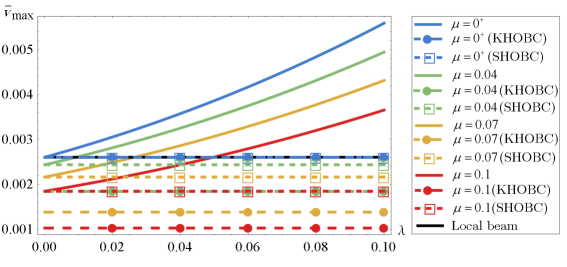
Figure 1:

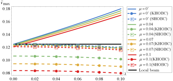
Figure 2:

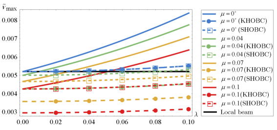
Figure 3:

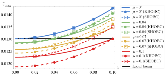
Figure 4:

References

- [1] Patti A, Barretta R, Marotti de Sciarra F, Mensitieri G, Menna C, Russo P. Flexural properties of multi-wall carbon nanotube/polypropylene composites: Experimental investigation and nonlocal modeling. Compos Struct 2015;131:282-89.
- [2] Acierno S, Barretta R, Luciano R, Marotti de Sciarra F, Russo P. Experimental evaluations and modeling of the tensile behavior of polypropylene/single-walled carbon nanotubes bers. Compos Struct 2017;174:12-18.
- [3] Kumar R, Singh R, Hui D, Feo L, Fraternali F. Graphene as biomedical sensing element: State of art review and potential engineering applications. Compos B Eng 2018;134:193-206.
- [4] Wang X, Jiang M, Zhou Z, Gou J, Hui D. 3D printing of polymer matrix composites: A review and prospective. Compos B Eng 2017;110:442-58.
- [5] Sedighi HM. Size-dependent dynamic pull-in instability of vibrating electrically actuated microbeams based on the strain gradient elasticity theory. Acta Astronaut 2014;95:111-123.
- [6] Koochi A, Sedighi H M, Abadyan M. Modeling the size dependent pull-in instability of beam-type NEMS using strain gradient theory. Latin American J Solids Struct 2014;11(10):1806-1829.
- [7] Sedighi HM. The influence of small scale on the pull-in behavior of nonlocal nanobridges considering surface effect, casimir and van der Waals attractions. Int J Appl Mech 2014;06(03):1450030.
- [8] Sedighi HM, Daneshmand F, Zare J. The influence of dispersion forces on the dynamic pull-in behavior of vibrating nano-cantilever based NEMS including fringing field effect. Arch Civil Mech Eng 2014;14(4):766-775.
- [9] Sedighi HM., Keivani M, Abadyan M. Modified continuum model for stability analysis of asymmetric FGM double-sided NEMS: Corrections due to finite conductivity, surface energy and nonlocal effect. Compos Part B 2015;83:117-133.
- [10] Sedighi HM, Shirazi KH. Dynamic pull-in instability of double-sided actuated nano-torsional switches. Acta Mech Solida Sinica 2015;28(1):91-101.
- [11] Sedighi HM, Daneshmand F, Abadyan M. Modeling the effects of material properties on the pull-in instability of nonlocal functionally graded nano-actuators. Z Angew Math Mech 2016;96:385-400.
- [12] Abadian F, Soroush R, Yekrangi A. Electromechanical Performance of NEMS Actuator Fabricated from Nanowire under quantum vacuum fluctuations using GDQ and MVIM. J Applied Computational Mech 2017;3(2):125-134.
- [13] Miandoab EM, Pishkenari HN, Yousefi-Koma A, Tajaddodianfar F, Ouakad H. Size Effect Impact on the Mechanical Behavior of an Electrically Actuated Polysilicon Nanobeam based NEMS Resonator. J Applied Computational Mech 2017;3(2):134-143.
- [14] Ghommem M, Nayfeh AH, Choura S, Najar F, Abdel-Rahman EM. Modeling and performance study of a beam microgyroscope. J Sound Vib 2010;329(23):4970-4979.
- [15] Farokhi H, Ghayesh MH. Nonlinear mechanics of electrically actuated microplates. Int J Eng Sci 2018;123:197-213.
- [16] Mojahedi M, Rahaeifard M. A size-dependent model for coupled 3D deformations of nonlinear microbridges. Int J Eng Sci 2016;100:171-182.
- [17] Bruno D, Greco F, Lonetti P, Blasi PN, Sgambitterra G, An investigation on microscopic and macroscopic stability phenomena of composite solids with periodic microstructure. Int J Solids Struct 2010;47(20):2806-2824.
- [18] Greco F, Luciano R. A theoretical and numerical stability analysis for composite micro-structures by using homogenization theory. Composites Part B 2011;42(3):382-401.
- [19] Greco F. A study of stability and bifurcation in micro-cracked periodic elastic composites including self-contact. Int J Solids Struct 2013;50(10):1646-1663.
- [20] Greco F, Leonetti L, Luciano R, Nevone Blasi P, Effects of microfracture and contact induced instabilities on the macroscopic response of finitely deformed elastic composites. Composites Part B 2016;107:233-253.
- [21] Barretta R, Marotti de Sciarra F. A Nonlocal Model for Carbon Nanotubes under Axial Loads. Adv Materials Sci Eng 2013(Article number: 360935);2013:1-6.
- [22] Čanadija M, Barretta R., Marotti de Sciarra M. On functionally graded Timoshenko nonisothermal nanobeams Composite Struct. 2016;135:286-296.
- [23] Barretta R, Brcic M, Čanadija M, Luciano R, Marotti de Sciarra F. Application of gradient elasticity to armchair carbon nanotubes: Size effects and constitutive parameters assessment. Eur. J. Mech. A. Solids 2017; 65: 1-13.
- [24] Akgöz B, Civalek Ö. Effects of thermal and shear deformation on vibration response of functionally graded thick composite microbeams. Composites Part B 2017;129:77-87.
- [25] Mercan K, Civalek Ö. Buckling analysis of Silicon carbide nanotubes (SiCNTs) with surface effect and nonlocal elasticity using the method of HDQ. Composites Part B 2017;114:34-45.
- [26] Faghidian SA. Integro-differential nonlocal theory of elasticity. Int J Eng Sci 2018;129:96-110.
- [27] Faghidian SA. On non-linear exure of beams based on non-local elasticity theory. Int J Eng Sci 2018;124:49-63.
- [28] Eltaher MA, Agwa M, Kabeel A. Vibration Analysis of Material Size-Dependent CNTs Using Energy Equivalent Model. J Applied Computational Mech 2018;4(2):75-86
- [29] Zhang DP, Lei Y, Shen ZB. Semi-Analytical Solution for Vibration of Nonlocal Piezoelectric Kirchhoff Plates Resting on Viscoelastic Foundation. J Applied Computational Mech 2018;4(3):202-215.
- [30] Karami B, Shahsavari D, Janghorban M, Li L. Wave dispersion of mounted graphene with initial stress. Thin-Walled Structures 2018;122:102-11.
- [31] Marotti de Sciarra F. Variational formulations and a consistent finite-element procedure for a class of nonlocal elastic continua. Int J Solids Struct 2008;45(14-15):4184-4202.
- [32] Marotti de Sciarra F. A nonlocal model with strain-based damage. Int J Solids Struct 2009; 46 (22-23):4107-4122.
- [33] Marotti de Sciarra F. Novel variational formulations for nonlocal plasticity Int J Plasticity 2009;25(2):302-331.
- [34] Romano G, Barretta R. Stress-driven versus strain-driven nonlocal integral model for elastic nano-beams. Composites Part B 2017;114:184-188.
- [35] Eringen AC. On differential equations of nonlocal elasticity and solutions of screw dislocation and surface waves. J Appl Phys 1983;54:4703-10.
- [36] Romano G, Barretta R, Diaco M, Marotti de Sciarra F. Constitutive boundary conditions and paradoxes in nonlocal elastic nano-beams. Int J Mech Sci 2017;121:151-56.
- [37] Barati MR. On wave propagation in nanoporous materials. Int J Eng Sci 2017;116:1-11.
- [38] Sahmani S, Aghdam MM. Nonlocal strain gradient beam model for postbuckling and associated vibrational response of lipid supramolecular protein micro/nano-tubules. Math Biosci 2018;295:24-35.
- [39] Romano G, Barretta R. Comment on the paper ”Exact solution of Eringen’s nonlocal integral model for bending of Euler-Bernoulli and Timoshenko beams” by Meral Tuna & Mesut Kirca. Int J Eng Sci 2016;109:240-42.
- [40] Barretta R, Diaco M, Feo L, Luciano R, Marotti de Sciarra F, Penna R. Stress-driven integral elastic theory for torsion of nano-beams. Mech Res Commun 2018;87:35-41.
- [41] Romano G, Barretta R. Nonlocal elasticity in nanobeams: the stress-driven integral model. Int J Eng Sci 2017;115:14-27.
- [42] Apuzzo A, Barretta R, Luciano R, Marotti de Sciarra F, Penna R. Free vibrations of Bernoulli-Euler nano-beams by the stress-driven nonlocal integral model. Compos B Eng 2017;123:105-11.
- [43] Mahmoudpour E, Hosseini-Hashemi, SH, Faghidian SA. Non-linear vibration analysis of FG nano-beams resting on elastic foundation in thermal environment using stress-driven nonlocal integral model. Appl Math Model 2018;57:302-15.
- [44] Barretta R, Čanadija M, Feo L, Luciano R, Marotti de Sciarra F, Penna R. Exact solutions of inflected functionally graded nano-beams in integral elasticity. Compos B Eng 2018;142:273-86.
- [45] Barretta R, Čanadija M, Luciano R, Marotti de Sciarra F. Stress-driven modeling of nonlocal thermoelastic behavior of nanobeams. Int J Eng Sci 2018;126:53-67.
- [46] Lim C. W, Zhang G, Reddy JN. A higher-order nonlocal elasticity and strain gradient theory and its applications in wave propagation. J Mech Phys Solids 2015;78:298-313.
- [47] Li L, Li X, Hu Y. Free vibration analysis of nonlocal strain gradient beams made of functionally graded material. Int J Eng Sci 2016;102:77-92.
- [48] Xu XJ, Wang XC, Zheng ML, Ma Z. Bending and buckling of nonlocal strain gradient elastic beams. Compos Struct 2017;160:366-77.
- [49] Barretta R, Marotti de Sciarra F. Constitutive boundary conditions for nonlocal strain gradient elastic nano-beams. Int J Eng Sci 2018;130:187-198.