Approximate optimization of MAXCUT with a local spin algorithm

Abstract

Local tensor methods are a class of optimization algorithms that was introduced in [Hastings, arXiv:1905.07047v2]Hastings (2019) as a classical analogue of the quantum approximate optimization algorithm (QAOA). These algorithms treat the cost function as a Hamiltonian on spin degrees of freedom and simulate the relaxation of the system to a low energy configuration using local update rules on the spins. Whereas the emphasis in Hastings (2019) was on theoretical worst-case analysis, we here investigate performance in practice through benchmarking experiments on instances of the maxcut problem. Through heuristic arguments we propose formulas for choosing the hyperparameters of the algorithm which are found to be in good agreement with the optimal choices determined from experiment. We observe that the local tensor method is closely related to gradient descent on a relaxation of maxcut to continuous variables, but consistently outperforms gradient descent in all instances tested. We find time to solution achieved by the local tensor method is highly uncorrelated with that achieved by a widely used commercial optimization package; on some maxcut instances the local tensor method beats the commercial solver in time to solution by up to two orders of magnitude and vice-versa. Finally, we argue that the local tensor method closely follows discretized, imaginary-time dynamics of the system under the problem Hamiltonian.

Binary unconstrained optimization, i.e., the maximization of an objective function on the configuration space of binary variables, is an important NP-hard optimization problem whose restrictions include several problems from Karp’s list of 21 NP-complete problems Karp (1972). Due to the hardness of the problems, many solution approaches rely on finding approximately optima in the shortest possible time, or constructing algorithms that have an optimality guarantee but without guarantees on runtime. Algorithms in the latter category are often referred to as exact solvers, and include approaches that use linear, quadratic, or semi-definite programming (LP/QP/SDP) relaxations of the problem instance with techniques to obtain optimality bounds such as cutting planes, branch-and-bound, or Langrangian dual-based techniques. While the design of exact algorithms may be well-suited to theoretical analysis, the runtime scaling in instance size is often poor.

In some cases, it is possible to design polynomial-time algorithms with guarantees on the approximation ratio, i.e., the ratio of the optimum obtained to the global maximum. These are, however, ultimately limited by hardness results on achieving approximation ratios above a certain threshold value Håstad (2001).

In the absence of runtime or optimality guarantees, problem-specific heuristics can nevertheless perform better than expected, exhibiting superior performance in runtime, optimality or both. An important class of heuristics takes inspiration from physical processes seen in nature, and those in this category that mimic the evolution of quantum systems are known as quantum-inspired optimization methods.

Quantum-inspired (or “dequantized”) algorithms have arisen in recent years of out a rich interplay between physics and algorithms research in the context of quantum computing. Thus, as notions of complexity now find analogues in many-body systems, so do quantum dynamics inform the design of quantum and classical algorithms. In the area of classical optimization, two quantum algorithms have generated considerable interest: quantum annealing and the quantum approximate optimization algorithm (QAOA). Promising developments in quantum annealing have inspired classical heuristic algorithms such as simulated quantum annealing Crosson and Harrow (2016) and sub-stochastic monte carlo Jarret et al. (2016), both of which mimic the evolution of the quantum state under an adiabatically evolving Hamiltonian.

Recent results on the performance of shallow-depth QAOA on the problem of max-e3-lin2 led to improved approximations of corresponding classical algorithms for the same problem Farhi et al. (2014); Barak et al. (2015). More recently, a new classical heuristic known as Local Tensor (lt) was introduced in Hastings (2019), taking inspiration from QAOA and closely related to previously known classical heuristics for distributed computing Hirvonen et al. (2014). It was shown in Hastings (2019) that lt has average-case performance better than single-layer QAOA for triangle-free maxcut and max-k-lin2 by tuning only one global hyperparameter, in contrast to the two-parameter tuning required for QAOA. Currently, it is unknown whether lt may be useful as a heuristic more broadly, and if so, how the hyperparameters should be set in practice. In this paper, we address this question by implementing a version of lt and benchmarking it on the problem of maxcut. We find that on the instances studied, the performance of lt can be considerably enhanced by hyperparameter tuning, and that it is possible to provide good initial guesses on the hyperparameters as function of the instance description. Under such settings, the performance of lt is comparable to the performance of the commercially available solver, Gurobi.

Our setup is described in Sections I, II and III, followed by a discussion of hyperparameter tuning and the underlying physics of the solver in Sections IV and V, respectively. Then, we compare the performance of tuned lt with those of Gurobi (Section VI) and gradient descent (Section VII). Finally, Section VIII discusses the similarity of our implementation of lt to discrete, imaginary-time Schrödinger evolution of the spin system under the problem Hamiltonian.

I  Spin problems

We refer to binary unconstrained optimization problems on spin degrees of freedom $s_{i}\in\left\{-1,1\right\}$ as spin problems. Most generally, one can express the objective function as a polynomial in the variables. Furthermore, since higher powers of the binary variables are trivial, the polynomial is guaranteed to be degree at most one in each variable. The objective function to be maximized can therefore be viewed (up to a negative sign) as a Hamiltonian of a spin system, and the optimization problem maps to sampling from the ground state of the Hamiltonian. The cost Hamiltonian for a system of $n$ spins with indices $\left\{1,2,\ldots,n\right\}$ can be written as

$$H=\sum\limits_{\alpha}w_{\alpha}\prod\limits_{i\in\alpha}s_{i}.$$ (1)

Therefore, $H$ is a sum of monomials, or clauses, where a clause $\alpha$ is supported on the subset of spins $\alpha\subseteq\left\{1,\ldots,n\right\}$. The sum is weighted by clause weights $w_{\alpha}$. The problem can be fully specified as a weighted hypergraph $G=(V,E,W)$, on vertices $V=\left\{1,2,\ldots,n\right\}$, hyperedges $E=\left\{\alpha,\cdots\right\}$, and clause weights $W=\left\{w_{\alpha},\ldots\right\}$.

A wide range of optimization problems be cast as binary unconstrained maximization problems Lucas (2014), making this problem description very versatile. A simple (and commonly studied) case is one where the polynomial (1) is quadratic, i.e. $|\alpha|\leq 2$ for every $\alpha$. This case captures several interesting physical systems such as Ising spin glasses, as well as a wide range of graph optimization problems. In this work, we focus on a particular quadratic spin problem, maxcut, defined in the following manner. Given a weighted graph $G=(V,E,W)$, we define a cut to be a partition of the vertices of the graph into two sets. The weight of the cut (or simply the cut) is then defined as the sum of weights of edges going across the cut. Therefore, for any $A\subset V$, the cut is

$$F(A):=\sum\limits_{i\in A,j\in\bar{A}}w_{ij}.$$ (2)

Then, given a graph $G$, maxcut asks for the largest cut of the graph. To show that maxcut can be written as a quadratic spin problem, we consider the following encoding: Assign a spin $s_{i}$ to vertex $i$. Then, there is a one-to-one mapping between bipartitions of $V$, $(A,\bar{A})$, and spin configuration, $\boldsymbol{\mathbf{s}}=\left(s_{1},s_{2},\ldots,s_{n}\right)$, namely, by setting $s_{i}=+1$ if $i\in A$ and $-1$ otherwise. Edges $ij$ that lie wholly in either $A$ or $\bar{A}$ do not count towards the cut, while edges between $A$ and $\bar{A}$ do. In terms of the spins, edge $ij$ will count towards the cut iff the spins $s_{i},s_{j}$ have opposite sign. Therefore, we may express the maxcut Hamiltonian in the following manner:

$$H_{\textsc{maxcut}{}} =\frac{1}{4}\sum\limits_{i,j}w_{ij}\cdot(s_{i}s_{j}-1).$$ (3)

$$\equiv\frac{1}{2}\boldsymbol{\mathbf{s}}^{T}\cdot J\cdot\boldsymbol{\mathbf{s}}$$ (4)

where $J_{ij}:=w_{ij}/2$ with zero diagonal terms, $J_{ii}=0$, and the last equivalence is an equality up to a constant offset $-\frac{1}{4}\sum\limits_{i,j}w_{ij}$. Notice that the ground state of $H_{\textsc{maxcut}{}}$ corresponds to the largest cut in $G$.

Despite its simple statement (and apparent similarity to the polynomial-time solvable problem of mincut), maxcut is known to be NP-hard Karp (1972). In fact, assuming the unique games conjecture holds, approximating maxcut to within a fraction 0.878.. is NP-hard. This is also the best known performance guarantee, achieved by the exact classical algorithm due to Goemans and Williamson (GW) on maxcut with non-negative weights. Custom solvers for maxcut that that improve on practical performance while sometimes preserving optimality are known Burer et al. (2002); Liers et al. (2004); Rendl et al. (2010).

maxcut is a well-studied problem and often used as a benchmark for new classical, quantum, and quantum-inspired solvers. Benchmarking of certain quantum-inspired optimization methods such as the coherent Ising machine Wang et al. (2013) and the unified framework for optimization or UFO (see, e.g., Mandrà et al. (2016)) has yielded promising results. In the following section, we discuss the lt heuristic framework and set up our implementation of the algorithm.

II  Local Tensor framework

Before describing our implementation, we review the local tensor (lt) algorithm framework laid out in Hastings (2019). The lt framework provides a general prescription for a class of local algorithms for the optimization of a Hamiltonian on spin variables. In a local algorithm, the state (e.g., a spin configuration) is encoded into the nodes of a graph, and the update rule at every node is local in the graph structure, depending only on nodes that are at most a bounded distance away. Local state updates therefore require information transfer among small neighborhoods and not the entire graph. If the graph has bounded degree, this can provide polynomial savings in the running cost of the algorithm. Additional speedup can be obtained in a true distributed model of computing where each node is an individual processor, and communication among nodes is slow compared to the internal operations of each processor.

lt is a local algorithm framework for optimization problems on spin degrees of freedom (such as maxcut). In lt, we first relax the domain of every spin variable from the binary set $\left\{-1,1\right\}$ to a continuous superset such as the real interval $[-1,1]$. By convention, we denote soft spins (i.e. those in the continuous domain) by letters $u,v$, etc. and hard spins by letters $r,s$, etc. Then, lt simulates dynamics of a soft spin vector $\boldsymbol{\mathbf{v}}$ in discrete time steps, and, at the end of a total number of steps $p$, retrieves a hard spin configuration $\boldsymbol{\mathbf{s}}$ from the final state via a rounding procedure applied to the soft spins. There is considerable flexibility in this setup, and for ease of study, we construct a specific instance of lt here.

Suppose we are given a maxcut instance whose corresponding Hamiltonian (as in (4)) is $H$. Denote the state of spin $i$ at time $t$ by $v_{i,t}$, and the full state vector by $\boldsymbol{\mathbf{v}}_{t}=\left(v_{1,t},v_{2,t},\ldots,v_{N,t}\right)$. Then, we perform the following steps in order, simultaneously for all spins $i=1,\ldots,N$.

1. Initialize all spins uniformly at random, $v_{i,0}\in[-1,1]$.

2. For $t=0,1,\ldots,p-1$, update $v_{i,t}\mapsto v_{i,t+1}$ as below:

   1. $v_{i,t.5}=v_{i,t}+cF_{i,t}$ where $F_{i,t}:=-\partial H/\partial v_{i,t}$ and $c$ is a real constant.

   2. $v_{i,t+1}=\tanh(\beta v_{i,t.5})$, where $\beta$ is a positive constant.

3. After $p$ rounds, round each spin to its sign, $v_{i,p}\mapsto\bar{s}_{i}=\mathrm{sgn}\left(v_{i,p}\right)\in\left\{-1,1\right\}$. Return $\bar{s}_{i}$.

The final configuration $\boldsymbol{\mathbf{\bar{s}}}$ is a feasible solution candidate. As there the initial configuration $\boldsymbol{\mathbf{v}}_{0}$ is sampled at random, an outer loop carries out several independent runs of the algorithm and selects the best solution.

For an instance of size $n$, the domain of feasible solutions corresponds to the vertices of an $n$-dimensional hypercube. The relaxation in lt extends the domain to the full hypercube, which allows for small, incremental updates and a well-behaved cost function, at the cost of making the search space infinite. However, the rounding step at the end of the algorithm offsets this drawback in the form of a lenient rounding rule: Return the nearest vertex of the hypercube. Therefore, the final state of the graph is only required to lie in the correct quadrant (or $2^{n}$-ant, to be precise) in order to produce the optimal solution.

The spin update sequence is carried out for a total of $p$ rounds, each consisting of two steps. The force $F_{i}=\partial H/\partial v_{i}$, calculated for each spin, displaces the spin by an amount proportional to it. We refer to the constant of proportionality $c$ as the response. Next, we apply the nonlinear function $\tanh(\beta v)$ to the spin, with a rescaling factor $\beta$ which we will call the inverse temperature. The number of rounds $p$, response $c$, and the inverse temperature $\beta$ form the hyperparameters of the algorithm, which must be fixed (ideally by optimization) before the algorithm is run on an instance. In theory, the factors $c,\beta$ can also be made to vary by round under a predetermined or adaptive schedule, in a manner similar to simulated annealing. Here, however, we will consider them to be constant in time.

III  The instances

Several open-access repositories for maxcut benchmarking instances are available online. In this work, we use the “Biq Mac” library Wiegele (2007). The maxcut instances provided here are random graphs with edge weights drawn from a certain probability distribution. Instances are categorized by the number of variables $n$, edge density $d$ (i.e. the expected number of non-zero weight edges) and the edge weight distribution used.

We organize these benchmarking instances in  Table 1.

Problem type	Weight distribution	$n$	$d$	Other
g05_$n$	$w_{ij}\in\left\{0,1\right\}$	$60,80,100$	$0.5$	–
pm1s_$n$	$w_{ij}\in\left\{-1,0,1\right\}$	$80,100$	$0.1$	–
pm1d_$n$	$w_{ij}\in\left\{-1,0,1\right\}$	$80,100$	$0.5$	–
w$d$_$n$	$w_{ij}\in\left[-10,10\right]$	$100$	$0.1,0.5,0.9$	–
pw$d$_$n$	$w_{ij}\in\left[0,10\right]$	$100$	$0.1,0.5,0.9$	–
ising$\sigma$-_$n$	$w_{ij}\propto\frac{\epsilon_{ij}}{|j-i|^{\sigma}}$, $\epsilon_{ij}\sim\mathcal{N}(0,1)$	$100,150,200,250,300$	–	$\sigma=2.5,3.0$
t$D$g$n^{1/D}$	$D$-dim. toroidal grid, $w_{<ij>}\in\left\{-1,1\right\}$	$5^{D},6^{D},7^{D}$	$\frac{2D}{n-1}$	$D=2,3$

Table 1: The benchmarking problems. Each instance is a random graph on $n$ vertices whose edge weights are chosen from the given distribution. In many cases, the overall density of clauses $d$, or, the ratio of non-zero weight edges, is fixed. The last two instances are random spin models borrowed from physics. The ising instances are a 1-dimensional Ising model with long-ranged interactions falling off as a power $\sigma$ of the inter-spin distance, with a numerator randomly sampled from the normal distribution. Finally, the t$D$g instances are periodic, $D$-dimensional spin lattices with random couplings $\pm 1$ along the edges of the lattice.

IV  Hyperparameter optimization

In order to talk about the performance of lt on any given instance, we must first consider variations in performance due to parameter setting and randomness. lt (as implemented here) is a family of algorithms in the hyperparameters $c,\beta,p$. Moreover, for fixed hyperparameters, any run of the algorithm has randomness due to the choice of initial spin configuration. Therefore, the energy output at the end of a single run of lt is a random variable dependent on $\left(c,\beta,p\right)$. The median final energy with fixed hyperparameters, however, is a determinate quantity, which we denote $E_{c,\beta,p}$.

$$E_{c,\beta,p}=\mathrm{median}_{\boldsymbol{\mathbf{v}}_{0}\in\left[-1,1\right]^{\times n}}\textsc{lt}{}_{c,\beta,p}(\boldsymbol{\mathbf{v}}_{0})$$ (5)

where, by abuse of notation, $\textsc{lt}{}(\boldsymbol{\mathbf{v}})$ denotes the output energy of lt with input configuration $\boldsymbol{\mathbf{v}}$. By definition, half of the runs of LT are expected to produce an optimum with energy lower than $E$, making the median energy a useful figure of merit. The true median energy can be approximated in practice by the median value of $M$ independent runs of $\textsc{lt}{}_{c,\beta,p}$,

$$\mathrm{median}\left\{E_{1},E_{2},\ldots,E_{M}\right\}=\tilde{E}\approx E_{c,\beta,p}$$ (6)

Since we ultimately wish to study the performance of LT as a whole, the hyperparameters must be fixed via a well-defined procedure that takes as input the instance description and returns an (ideally optimal) hyperparameter setting. The most rigorous criterion is global optimization of the performance with respect to each hyperparameter independently. This is important, e.g. to avoid spurious trends in the runtime scaling that arise from imperfect hyperoptimization.

Since this is a computationally expensive task, we focus first on gaining a better understanding of the effect of the hyperparameter on the algorithm performance, and construct metaheuristics to minimize the resources needed for hyperparameter optimization.

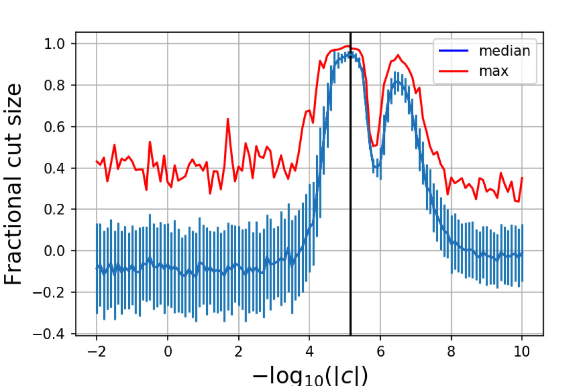
Figure 1: Hyperparameter sweep for the instance ising2.5-100. We vary $c$ over multiple orders of magnitude, and plot the median and max value of optimum found for several runs of the algorithm. It can be seen that peak performance is found when $c\sim\bar{c}$ (indicated by the black line).

Response $c$.

The response $c$ is the sensitivity of the spins to force. Intuitively, setting $c$ too large or too small would make the spins too responsive to displacement or frozen, respectively.

Therefore, we expect a regime for $c$ values where the spins are optimally sensitive to the force, and the algorithm should also perform well in this regime. Given a typical length of spins $v_{i}\sim 1$ and maximum possible force on spin $i$, $F_{i}\sim\sum\limits_{j=1}^{N}|J_{ij}|$, a natural guess for $c$ is the inverse of the maximum force. We define

$$\bar{c}=2\left\langle\sum\limits_{j=1}^{N}|J_{ij}|\right\rangle_{i}^{-1}$$ (7)

where the brackets $\langle\cdot\rangle_{i}$ denote a mean over all sites in the graph. The factor of two is chosen purely empirically. As shown in Fig. 1, we find that $\bar{c}$ is indeed a natural scale for the response, and optimal performance is typically found to be within an order 1 factor of $\bar{c}$. Hereafter, we use a rescaled hyperparameter $\eta:=c/\bar{c}$.

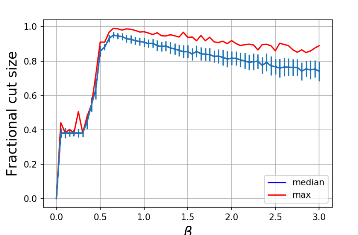
Figure 2: Hyperparameter sweep for the instance ising2.5-100. We plot the median (blue) and max (red) performance as a function of $\beta$, for a fixed value of $c\sim\bar{c}$. The performance is sensitive to order 1 variation in $\beta$, varying from sub-random (cut fraction $0.5$) to close to optimal at $\beta\simeq 0.7$. This behavior is typical across all instances studied.

Inverse temperature $\beta$.

The $\beta$ parameter scales the value of the input to the $\tanh$ activation function. Intuitively, this enables mapping the displaced spin to the linear response region of the $\tanh$ function for maximum sensitivity. This also ensures that the spin stays of order 1 and therefore sensitive to forces applied in subsequent rounds.

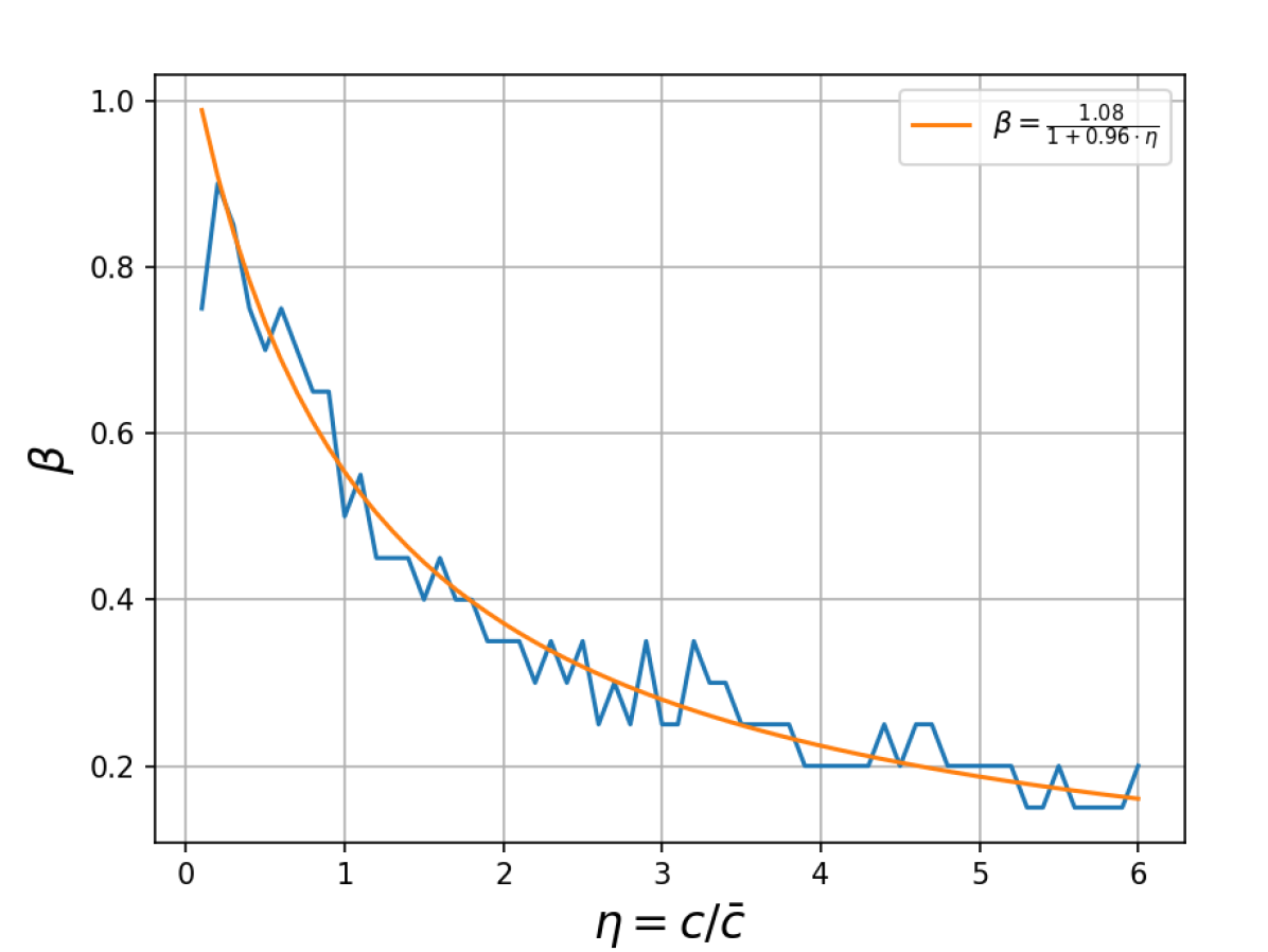
Figure 3: Optimal $\beta$ for a range of $\eta$ values, plotted for a torus instance. For each $\eta$, the optimal $\beta$ was found by grid search. The fit to the functional form given in (8) is also shown. The curve profile and quality of fit seen here are typical to all instances studied.

Just like the response, we can now make an educated guess for $\beta$. For a fixed response $\eta=c/\bar{c}$, spin $v_{i}$ is displaced as $v_{i}\rightarrow\tanh{\beta(v_{i}+cF_{i})}$. Since $v_{i}\leq 1$ for all $i$, the argument of the tanh function must lie between $[-\beta(1+\eta),+\beta(1+\eta)]$. In order to be maximally sensitive to displacement, we should set $\beta$ such that $\beta(1+\eta)\sim O(1)$. This gives us a functional dependence between $\beta$ and $\eta$ as

$$\beta=\frac{a}{1+b\eta},$$ (8)

where we have introduced two fitting parameters $a,b$. From the available instances, this relationship can be checked by extracting the locus of optimal settings for $(\eta,\beta)$ and fitting them to the above functional form. The results are shown in Fig. 3. The quality of fits suggests that the functional dependence given in  Eq. 8 is accurate. In Fig. 4, we show how the coefficients $a,b$ cluster for different problems.

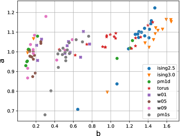
Figure 4: Clustering in the fit coefficients $a,b$ in (8) for different instances (see Table 1). We see that the fitting numerator $a$ is close to 1 for most instances, while $b$ varies considerably. There is a reasonable degree of clustering by instance type in $b$.

From this analysis, we see that given a problem instance, the hyperparameters $\eta,\beta$ can be guessed with very little optimization, and tuned further, if necessary, by local search in a range of order 1 in each parameter.

Number of rounds $p$.

The number of rounds $p$ required by the algorithm is dictated by the convergence to steady state. Qualitatively, this may be connected to the rate of information propagation in the graph, via quantities such as the girth. Unlike for $c,\beta$ however, a direct guess for $p$ may be harder to obtain.

Instead, we use a dynamic criterion to set the value of $p$. Since lt is iterative and closely related over gradient descent, we expect that at some point during the algorithm, the spin vector attains a steady state such that all subsequent displacements are smaller than a given threshold. As the final state is determined by the quadrant containing the vector and not the exact value of the vector, small displacements have a small or no effect on the outcome.

This convergence in the state vector is seen across different instances. Therefore, once the displacement of the state falls below a set threshold, we terminate the algorithm. While the threshold is an additional parameter, it can be set to be sufficiently smaller than the size of the hypercube.

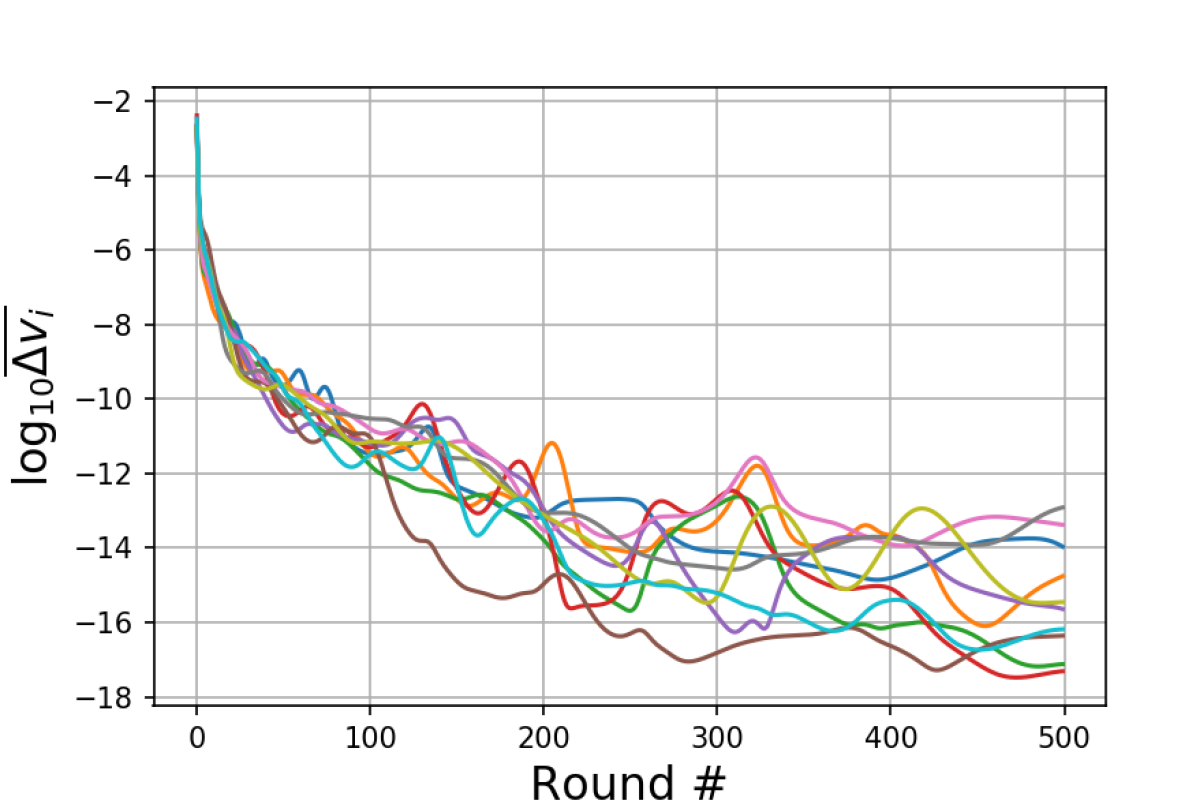
Figure 5: Displacement in the spin variables between successive rounds, as a function of round number. We have chosen ten spins from a 100-spin instance of type w05 for illustration. The log displacement becomes small after a short number of rounds, indicating that the updates can be terminated early for the rounding step.

V  Dependence of lt dynamics on the hyperparameters

The implementation of lt studied here allows three hyperparameters, namely, the number of rounds $p$, the response to force $c$, and the “inverse temperature" $\beta$. We have discussed how to set these hyperparameters for a given maxcut instance, giving (in the case of $c,\beta$) good initial approximations that depend on the instance description, or (in the case of $p$) a dynamic criterion based on the convergence of the state vector. Here we give a physical description of the system dynamics and show, qualitatively, why it is reasonable to expect such behaviors.

We will analyze the behaviour of lt near a steady state solution $\bar{v}$ that satisfies $\bar{v}_{i}=\tanh\left[\beta\left(\bar{v}_{i}+c\bar{F}_{i}\right)\right]$ for all spins $i$. Note that a steady state always exists: the all-zero state $\bar{v}_{i}=0$ is an example. More generally, the transcendental equation for steady state, while not guaranteed to have other solutions, can be approximated as a linear equation when $\bar{v}_{i}\ll 1$, which has non-zero solutions for particular values of $\beta,c$. Generically, we expect other steady solutions lying within the hypercube, and find this to be true in our numerics.

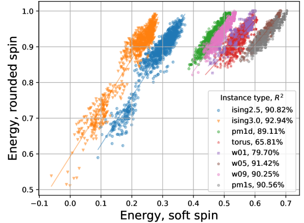
Figure 6: We plot the objective function evaluated at the soft spin (y axis) and the corresponding rounded spin obtained at the end of an lt run, for several independent runs of the algorithm on eight instances. Each instance is picked from a different instance type. The correlation between the two quantities (given by $R^{2}$ values in the legend) indicates that better steady state soft spin configurations tend to map to better feasible solutions.

Suppose, for a given run of the algorithm, the system tends to a particular steady state $\bar{v}$ at long times, with the state at some finite time $t$ given by $\boldsymbol{\mathbf{v}}_{t}=\boldsymbol{\mathbf{\bar{v}}}+\boldsymbol{\mathbf{\delta}}_{t}$, where $|\delta_{i,t}|\ll|\bar{v}_{i}|$. Then, to first order in the displacement, we have

$$v_{i,t+1} =\tanh\left[\beta\left[\left(\mathbbm{1}+cJ\right)\cdot\left(\boldsymbol{\mathbf{\bar{v}}}+\boldsymbol{\mathbf{\delta_{t}}}\right)\right]_{i}\right]$$ (9)

$$=\tanh\left[\beta\left(\bar{v}_{i}+c\bar{F}_{i}\right)+\beta\left[\left(\mathbbm{1}+cJ\right)\cdot\boldsymbol{\mathbf{\delta}}\right]_{i}\right]$$ (10)

$$\simeq\tanh\left[\beta\left(\bar{v}_{i}+c\bar{F}_{i}\right)\right]$$ (11)

$$+ \beta\left[\left(\mathbbm{1}+cJ\right)\cdot\boldsymbol{\mathbf{\delta}}\right]_{i}\mathrm{sech}^{2}\left[\beta\left(\bar{v}_{i}+c\bar{F}_{i}\right)\right]$$ (12)

$$=\bar{v_{i}}+\beta\left(1-\bar{v}_{i}^{2}\right)\left[\left(\mathbbm{1}+cJ\right)\cdot\boldsymbol{\mathbf{\delta}}\right]_{i}$$ (13)

where we used the steady-state condition, and $\tanh^{\prime}(x)=1-\tanh^{2}(x)$. Therefore, the displacement at time $t+1$ is

$$\boldsymbol{\mathbf{\delta}}_{t+1}\simeq\beta\left(\mathbbm{1}-\bar{V}^{2}\right)\cdot\left(\mathbbm{1}+cJ\right)\cdot\boldsymbol{\mathbf{\delta}}_{t}\,,$$ (14)

where we defined the diagonal matrix $\bar{V}_{ii}=\bar{v}_{i}$. Therefore, the norm of the displacement vector close to steady state is bounded as

$$|\boldsymbol{\mathbf{\delta}}_{t+1}|\lesssim|\beta|\cdot||\left(\mathbbm{1}-\bar{V}^{2}\right)||\cdot||\left(\mathbbm{1}+cJ\right)||\cdot|\boldsymbol{\mathbf{\delta}}_{t}|\,.$$ (15)

Since $||\left(\mathbbm{1}-\bar{V}^{2}\right)||\leq 1$, and $||\mathbbm{1}+cJ||\leq 1+|c|\cdot||J||$, it follows that

$$|\boldsymbol{\mathbf{\delta}}_{t+1}|\lesssim\beta\cdot\left(1+c||J||\right)\cdot|\boldsymbol{\mathbf{\delta}}_{t}|\,,$$ (16)

assuming $c,\beta\geq 0$. Finally, consider the following properties:

1. Since $J$ has zero diagonal, then by the Gershgorin circle theorem, all eigenvalues of $J$ lie within a disc of radius $\max_{i}\sum\limits_{j=1}^{n}|J_{ij}|$.

2. If $c=\eta\bar{c}$, where $\bar{c}=\max_{i}\sum\limits_{j=1}^{n}|J_{ij}|$, then $1+c||J||\leq 1+\eta$.

Therefore, for a choice $\beta\gtrsim\frac{1}{1+\eta}$, we expect

$$|\boldsymbol{\mathbf{\delta}}_{t+1}|\lesssim|\boldsymbol{\mathbf{\delta}}_{t}|$$ (17)

giving the condition for dynamics converging to a steady state. Three observations can be drawn from this:

1. $\bar{c}$ provides a natural unit for the response $c$.

2. For optimal convergence, we expect the dependence between $\beta$ and $\eta=c/\bar{c}$ to be given by $\beta\simeq a/(1+b\eta)$ for some parameters $a,b$.

3. Under the above circumstances, the trajectory near steady state is stable and follows an exponential convergence towards the steady state solution. Therefore, the algorithm can be “safely” terminated when the displacement is under a certain threshold.

These three observations closely match our empirically derived rules for good performance of lt. This indicates that the steady state solutions may also correlate with the locations of good feasible solutions (given by the nearest hypercube vertex). This can be seen in Fig. 6.

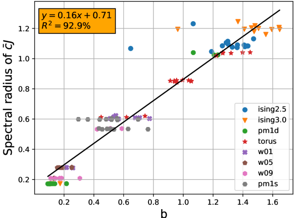
Figure 7: Dependence of the fitting parameter $b$ and the spectral radius of the the normalized coupling matrix $\bar{c}J$. A linear regression fits the data with $R^{2}=92.9\%$, indicating a strong linear relationship between the two quantities. Therefore, the spectral norm of the coupling matrix can give a good estimate on the fitting parameter $b$ and hence $\beta$.

In fact, the quantity $\bar{c}$ is defined not as the maximum but as a mean, Eq. 7. However, the functional relationship $\beta=\frac{a}{1+b\eta}$ is still seen to hold for some $a,b$.

We can study the dependence of $a,b$ by instance type. As shown in Fig. 4, the parameters form clusters by instance type, and the value of $a$ is close to 1 for all instances studied. The value of $b$ varies considerably from instance to instance. Looking at the functional form, it is reasonable to guess that $b$ is related to the spectral radius of the coupling matrix $J$. While we bound the magnitude of the largest eigenvalue by $\max_{i}\sum\limits_{j=1}^{n}|J_{ij}|$, the actual value may be smaller, and $b$ may be understood to reflect this correction. We check this conjecture by plotting the relationship between $||J||$ and $b$ for every problem instance in Fig. 7.

This relationship can be particularly useful if the largest eigenvalue of the matrix can be calculated or estimated quickly. Then, by inverting the linear regression shown in Fig. 7, one obtains a good initial guess for $b$. The initial guess for $a$, on the other hand, is simply 1. This potentially reduces the hyperparameter optimization to local minimization in the single parameter $\eta$, which is computationally inexpensive.

VI  Comparison with Gurobi

Gurobi is a versatile commercial optimization software that solves a broad range of problems including quadratic programming (QP), linear programming, and mixed integer programming. Additionally, the software includes in-built heuristics to find good initial solution candidates quickly, as well as “pre-solve” subroutines and simplify the problem description by eliminating redundant variables or constraints.

In order to use Gurobi, a maxcut instance can be relaxed to either a linear program or a quadratic program. Mapped to an LP, the instance is specified by real variables $x_{ij}\in\mathbb{R}$ to each edge, with the inequality constraints $x_{ij}\leq 1$, where $x_{ij}=1$ if and only if the edge $ij$ is in the cut. Additional constraints follow by observing that not all configurations are feasible: for example, for three edges $ij,jk,ki$, at most two may be part of a cut. Any feasible solution must satisfy such cycle constraints as well, expressible as inequalities of the form $x_{ij}+x_{jk}+x_{ki}\leq 2$. Then, the LP is formulated as maximization of the objective function $\boldsymbol{\mathbf{w}}^{T}\boldsymbol{\mathbf{x}}$, subject to the above inequalities, where $\boldsymbol{\mathbf{w}}$ represents the vector of edge weights. While the number of cycle inequalities are exponential, it is possible to solve the separation problem in polynomial time Barahona and Mahjoub (1986), leading to a cutting-planes algorithm for finding and including violated constraints dynamically for each successive iteration of the LP. However, this formulation is somewhat unnatural for maxcut, and is seen to perform poorly for dense graphs, due to a blowup in the number of variables.

A more natural formulation is as a QP with linear constraints, where every vertex $i$ is assigned to one variable $s_{i}$, and the problem is expressed as

$$\max~{}\frac{1}{4}\boldsymbol{\mathbf{s}}^{T}\cdot W\cdot\boldsymbol{\mathbf{s}}$$

$$\mathrm{s.t.}\ -1\leq s_{i}\leq 1.$$

Here, the matrix $W$ is the weighted graph Laplacian, with $w_{ii}=\sum\limits_{k\neq i}w_{ik}$ and $W_{ij}=-w_{ij}$ for $i\neq j$.

The QP formulation is convex when the edge weights are non-negative, and not otherwise. However, the weight matrix $W$ can be made convex trivially by the addition of a suitably chosen diagonal matrix $D$. Since we seek spin configurations that must satisfy $s_{i}^{2}=1$ for all spins $i$, the diagonal merely shifts the objective function by a constant everywhere on the feasible solutions. For a sufficiently large shift, the matrix becomes positive semi-definite by the Gershgorin circle theorem: All eigenvalues of $W+D$ lie in the union of all discs $S_{i}\in\mathbb{C}$ with centers given by $w_{ii}+D_{ii}$ and radii $\sum\limits|w_{ij}|$. Then $D_{ii}$ can always be chosen large enough so that each disc lies wholly in the right half-plane, so that all eigenvalues of $W-D$ are non-negative. This makes the shifted maximization problem convex, implying that solutions to the relaxed problem yield feasible solutions of the discrete problem.

Gurobi has support for both convex and non-convex QP, and uses interior point methods (specifically, a parallel barrier method) and the simplex method to solve problems in QP formulation. We provide the instances to Gurobi in QP formulation.

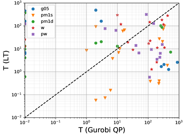
Figure 8: Performance of lt compared against Gurobi for several benchmarking instances. The performance metric used is median time taken to find the optimum (over 10 runs), with a timeout of $10^{3}$ seconds. Timed out instances are not shown: Out of 130 instances, LT and Gurobi timed out on 47 and 22 instances, respectively, including 7 instances where both timed out. Times faster than a certain threshold are reported by Gurobi as 0s (corresponding to points along the left edge). lt and Gurobi find optima faster than each other in an equal number of instances, with no clear instance-dependent advantange. The speedup on either side is in some cases up to three orders of magnitude.

Then, we can compare the time to find optimal solution for Gurobi and lt on our benchmarking instances. The time has to be carefully defined in each case for a fair comparison. Gurobi is a deterministic algorithm, except for an initial (optional) heuristic step for proposing an initial solution candidate which takes a small fraction of the total runtime. The algorithm terminates when the optimum is found and proved. The latter typically requires additional time to improve the upper bound on the optimum until it matches the best optimum found. Since we use benchmarking instances that have known optima, we define runtime leniently as the time to find (but not necessarily prove) the optimal solution.

On the other hand, lt is randomized due to the random choice of initial state, and multiple runs are necessary to gather statistics on the performance. Therefore, we define runtime as the median performance over 30 independent runs of lt for each instance. Furthermore, since lt requires parameter tuning, we allow up to 20 $s$ of hyperparameter tuning by grid search in $\beta,\eta$ that is not considered part of the runtime. Note that the results of Section IV suggest that the parameters can be set automatically, either adaptively as for $p$ or by a well-motivated formula for $\eta,\beta$, without the need for a full grid search.

Then, as shown in Fig. 8, the runtime performance of lt and Gurobi can be compared directly on every instance. We see that there is significant spread in performance for every problem type, for both lt and Gurobi. Promisingly, there are instances in every problem class for which lt is significantly faster than Gurobi.

The comparison with Gurobi illustrates that there may be cases where properly tuned LT can outperform state-of-the-art solvers at a fraction of the time cost. It is pertinant to ask whether the success of LT over other solvers can be predicted in advance, using instance data (or quantities derived from it). We briefly address this question.

The most obvious performance indicator is the number of variables $n$. The instances used in the time comparison with Gurobi were of size 60, 80, or 100. Another elementary indicator is clause density, or the mean number of clauses per variable, which for a weighted instance is the average row sum of the graph adjacency matrix, $m:=\sum\limits_{i,j}J_{ij}/n$. We also compute the average row sum of the absolute value of the weight matrix $\bar{m}:=\sum\limits_{i,j}|J_{ij}|/n$. Finally, the misfit parameter $\mu$ measures the degree of frustration in the model. More precisely, it is the ratio of the ground state energy of the model to the ground state energy of a frustration-free reference system. For a given maxcut instance, a reference system with all weights $J_{ij}$ replaced by their negative absolute values $-|J_{ij}|$ is frustration-free, with a ground state energy of $-\sum\limits_{i<j}|J_{ij}|$. On the other hand, the ground state energy of the original instance is bounded below by $-\sum\limits_{i<j}J_{ij}$. Therefore, we define misfit as

$$\mu:=\frac{\sum\limits_{i<j}J_{ij}}{\sum\limits_{i<j}|J_{ij}|}\,.$$ (18)

Then, we ask: How well does a given performance indicator predict the runtime of LT (or Gurobi) on a randomly chosen instance? More formally, treating the runtime and indicator as random variables $X,Y$ respectively, the predictive power can be expressed as the conditional entropy $H(Y|X)$, defined as

$$H(Y|X):=-\sum\limits_{x\in\mathcal{X},y\in\mathcal{Y}}p(x,y)\log\frac{p(x,y)}{p(x)}\,,$$ (19)

where the sum is taken over the support sets of $X,Y$. Informally, $H(Y|X)$ quantifies the number of additional bits needed to specify $X$ given knowledge of $Y$. The largest possible value of $H(Y|X)$ is $\log|\mathcal{X}|$ for a discrete sample space $\mathcal{X}$, corresponding in our case to the number of bins used to group the runtimes. We report the conditional entropy normalized by this maximum, so that a normalized entropy of $0$ ($1)$ corresponds to perfect (no) predictability. The results are presented in Table 2. Relative to Gurobi, the performance of LT is marginally more predictable using the instance data. However, clearly discernable relationships between the performance and any of the indicators studied here could not be obtained using the instance data available, suggesting the need for further systematic study.

Predictor		Gurobi	LT
$n$		0.73	0.69
$m$		0.68	0.63
$\bar{m}$		0.66	0.59
$\mu$		0.56	0.53

Table 2: A tabulation of the normalized conditional entropy (as defined in Eq. 19) of different performance predictors with the runtime of Gurobi and lt on the benchmarking instances. Zero indicates perfect prediction, while 1 corresponds to no predictability. The real-valued predictors $m,\bar{m},\mu$ were binned into 20 equally spaced intervals, and the runtime was binned into 20 logarithmic intervals spanning the range 0.01s to 1000 s, with an additional bin for timed-out instances ($t>1000$s).

VII  Comparison with Gradient Descent

An inspection of the lt implementation reveals that the algorithm is operationally very similar to a gradient descent algorithm. The difference lies only in the fact that we apply a nonlinear $\tanh$ wrapper to each spin value in every step, while gradient descent is fully linear. This raises a natural question: does lt offer any advantage to gradient descent?

We formalize this comparison. The maxcut Hamiltonian does not have a global extremum over $\mathbb{R}^{n}$, as all of its second (and higher-order) derivatives vanish. This implies that a gradient descent algorithm must constrain the state vector to lie within a closed region of $\mathbb{R}^{n}$; then the optima are guaranteed to lie on the boundary of this region. The natural choice of region is the $n$-dimensional hypercube $H_{n}:=[-1,1]^{\times n}$, whose vertices correspond to feasible solutions to the maxcut problem. Then, any step that displaces the state vector outside $H_{n}$ must be modified to obey the constraint. We implement this by applying a cutoff function to each spin at the end of every displacement step. The form of this function is as follows:

$$\mathrm{cutoff}(x)=\mathrm{sgn}(x)\cdot\min\left\{1,|x|\right\}.$$ (20)

When applied to each spin as $\mathrm{cutoff}(\beta v_{i})$, this function has the effect of projecting every spin component that exceeds an allowed range $[-1/\beta,1/\beta]$ onto the closest boundary of the range. The free parameter $\beta$ controls how wide the allowed range should be.

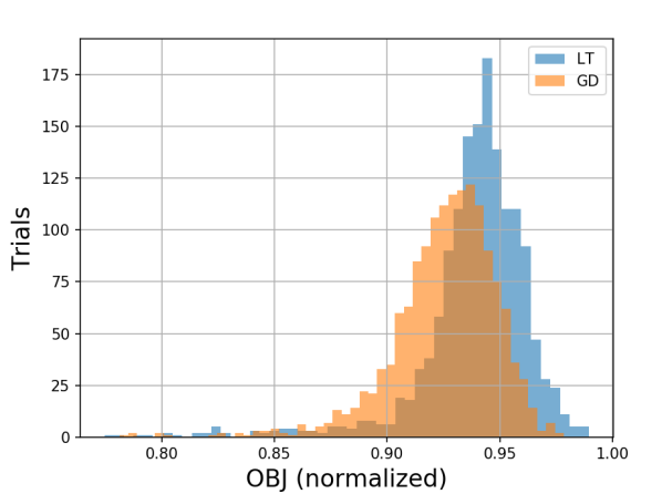
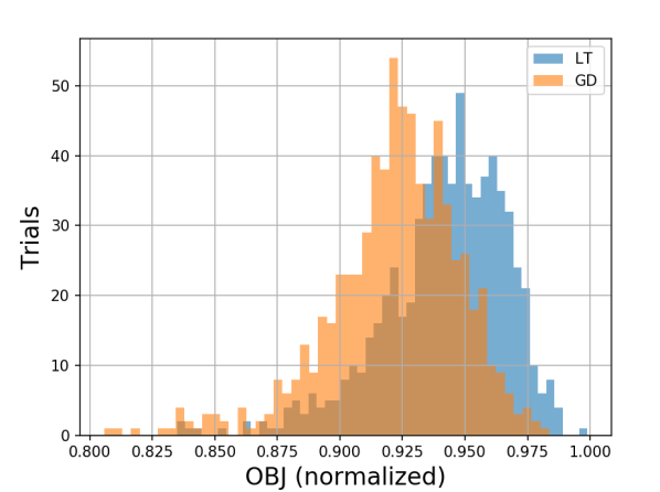
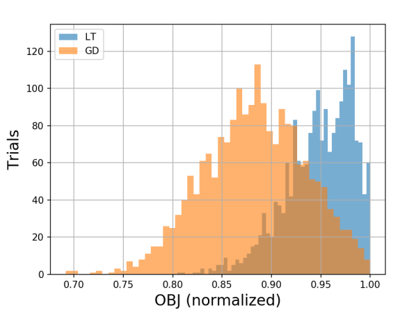
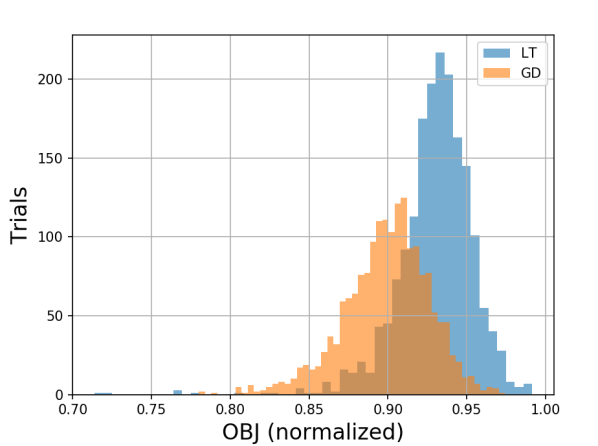
Figure 9: A comparison of lt and gradient descent for a selection of instances. We see that lt produces higher quality optima than gradient descent. For each instance, hyperparameters for both algorithms were tuned to maximize performance.

The full algorithm may then be written down:

1. Initialize all spins uniformly at random, $v_{i}\in[-1,1]$.

2. Apply displacement to spin $v_{i}\mapsto v_{i}+c\cdot F_{i}$ where $F_{i}=\partial H/\partial v_{i}$.

3. $v_{i}\mapsto\mathrm{cutoff}(\beta v_{i})$.

4. After $p$ rounds, round each spin to its sign, $\pm 1$.

It is now apparent that GD mirrors lt, with the difference lying in the choice of onsite activation function used: lt uses the tanh function while GD uses a hard cutoff function. Both algorithms have identical free parameters $p,c,\beta$ that play the same or similar functional roles in each case. Then, we can compare the performances of these algorithms on the same instances. In Fig. 9, we see that lt beats GD for the instances shown (and, in fact, all the benchmarking instances studied). This suggests that the specific form of lt that uses a tanh function offers an advantage over a hard cutoff function. In the next section, we motivate this choice further by drawing a parallel between lt and imaginary time-evolution the spins under the problem Hamiltonian.

VIII  LT as a discretized, imaginary-time Schrödinger evolution

Given any initial state $|\psi\rangle$ and Hamiltonian $H$, time-evolution of $|\psi\rangle$ under $H$ is given by the Schrödinger equation $d|\psi\rangle/dt=-iH|\psi\rangle$. The evolution applies a phase to the eigenstates of $H$ proportional to the energy of the state times time, so that low-energy states rotate slowly while highly excited states rotate fast. An analytical tool often employed to access the low-energy spectrum of $H$ is that of analytic continuation to imaginary time. In this, one replaces the time by an imaginary time parameter $\tau:=it$, and the (unnormalized) imaginary time Schrödinger equation reads

$$\dot{|\psi\rangle}\equiv d|\psi\rangle/d\tau=-H|\psi\rangle\,.$$ (21)

The formal solution to this equation is $|\psi(\tau)\rangle=e^{-H\tau}|\psi(0)\rangle$. Note that $|\psi(\tau)\rangle$ is unnormalized, but we keep track of the normalization $\mathcal{N}(|\psi(\tau)\rangle)\equiv\mathcal{N}(\tau):=\sqrt{\langle\psi(\tau)|\psi(\tau)\rangle}$. In the limit $\tau\rightarrow\infty$, and assuming that the ground state of $H$ is non-degenerate, the exponential $e^{-\tau H}$ suppresses contributions from all but the lowest-energy state $|\psi_{0}\rangle$ of $H$, which implies that $\lim_{\tau\rightarrow\infty}|\psi(\tau)\rangle=|\psi_{0}\rangle$.

The normalization $\mathcal{N}(\tau)$ has $\tau$-dependence

$$\dot{\mathcal{N}} =\frac{1}{2\sqrt{\langle\psi|\psi\rangle}}\cdot\left(\langle\dot{\psi}|\psi\rangle+\langle\psi|\dot{\psi}\rangle\right)$$ (22)

$$=-\frac{\langle H\rangle}{\mathcal{N}}$$ (23)

where $\langle H\rangle:=\langle\psi|H|\psi\rangle$ is the unnormalized expectation value of operator $H$. The normalized expectation value is given by $\langle\langle H\rangle\rangle:=\langle H\rangle/\mathcal{N}^{2}$.

Next, let $H$ be a Hamiltonian acting on $n$ qubits that is diagonal in the $Z$ basis. Any state $|\psi\rangle$ in this Hilbert space can be mapped to a vector of normalized expectation values of the Pauli operators $Z_{i}$, where the index $i$ runs over all spins:

$$|\psi(\tau)\rangle \mapsto\left(\langle\langle Z_{1}\rangle\rangle,\langle\langle Z_{2}\rangle\rangle,\ldots,\langle\langle Z_{n}\rangle\rangle\right)$$

$$=:\left(v_{1},v_{2},\ldots,v_{n}\right)\,,$$

where $v_{i}\in[-1,1]$ is the classical spin variable that tracks the normalized expectation of $Z_{i}$. The imaginary time-evolution of the spins is given by

$$\dot{v_{i}} =\frac{d}{d\tau}\left(\frac{\langle Z_{1}\rangle}{\mathcal{N}^{2}}\right)$$ (24)

$$=\frac{-2\dot{\mathcal{N}}}{\mathcal{N}^{3}}\langle Z_{i}\rangle+\frac{1}{\mathcal{N}^{2}}\frac{d}{d\tau}\langle\psi|Z_{i}|\psi\rangle\,,$$ (25)

$$=2v_{i}\langle\langle H\rangle\rangle-\langle\langle HZ_{i}+Z_{i}H\rangle\rangle\,.$$ (26)

This is essentially an imaginary-time analogue of the Ehrenfest theorem. Since Pauli operators $Z_{i}$ square to the identity, a diagonal Hamiltonian $H$ can always be written as

$$H=R_{i}Z_{i}+S_{i}\,,$$ (27)

for every site $i$, for some operators $R_{i},S_{i}$ that are not supported on site $i$. Then, $HZ_{i}=Z_{i}H=R_{i}+S_{i}Z_{i}$. Next, we make a mean-field assumption, $\langle\langle H_{\bar{i}}Z_{i}\rangle\rangle\approx\langle\langle H_{\bar{i}}\rangle\rangle\cdot\langle\langle Z_{i}\rangle\rangle$, where $H_{\bar{i}}$ is any local operator not supported on site $i$. Then, it follows that $\langle\langle HZ_{i}\rangle\rangle\approx\langle\langle R_{i}\rangle\rangle+v_{i}\cdot\langle\langle S_{i}\rangle\rangle$, and $\langle\langle H\rangle\rangle\approx v_{i}\cdot\langle\langle R_{i}\rangle\rangle+\langle\langle S_{i}\rangle\rangle$, which gives

$$\dot{v_{i}} =2\left(v_{i}^{2}\cdot\langle\langle R_{i}\rangle\rangle+v_{i}\langle\langle S_{i}\rangle\rangle-\langle\langle R_{i}\rangle\rangle+v_{i}\cdot\langle\langle S_{i}\rangle\rangle\right)$$ (28)

$$=-2\left(1-v_{i}^{2}\right)\cdot\langle\langle R_{i}\rangle\rangle\,.$$ (29)

Next, we make a substitution $u_{i}:=\tanh^{-1}v_{i}$ which maps the real line into the open interval $(-1,1)$. Then, $\dot{v}_{i}=1-\text{sech}^{2}(u_{i})\dot{u}_{i}=(1-v_{i}^{2})\dot{u}_{i}$, therefore we can write

$$\dot{u}_{i}=-2\langle\langle R_{i}\rangle\rangle.$$ (30)

Note now that the term $\langle\langle R_{i}\rangle\rangle$ is precisely the expected value of the force on spin $i$, since $dH/dZ_{i}=R_{i}$. Finally, an imaginary time evolution discretized into small time steps $\delta\tau$ obeys (in mean field)

$$v_{i}(\tau+\delta\tau)=-\tanh\left(2\delta\tau F_{i}+\tanh^{-1}v_{i}\right).$$ (31)

This equation bears similarity to the update rule for lt. In fact, for $v_{i}$ sufficiently small and close to steady state $\bar{v}_{i}$, we can expand the inverse tangent as $\tanh^{-1}v_{i}\approx v_{i}+v_{i}^{3}/3+\ldots\approx-2\bar{v}_{i}^{3}/3+v_{i}\cdot(1+\bar{v}_{i}^{2})$, which looks linear with a modified slope. This reveals a surprising connection between lt and a discretized, mean-field imaginary time evolution of classical spin expectation values.

Our analysis suggests a generalization of lt to situations where the Hamiltonian is not diagonal in the $Z$ basis. In this context, we can represent each spin $i$ as a 3D rotor $\boldsymbol{\mathbf{r}}_{i}=(x_{i},y_{i},z_{i})=\left(\langle\langle X_{i}\rangle\rangle,\langle\langle Y_{i}\rangle\rangle,\langle\langle Z_{i}\rangle\rangle\right)$ of Pauli expectation values. Since the Paulis square to the identity, a general spin Hamiltonian $H$ can always be written as

$$H=P_{i}X_{i}+Q_{i}Y_{i}+R_{i}Z_{i}+S_{i}\,,$$ (32)

for every site $i$, where $P_{i},Q_{i},R_{i},S_{i}$ are some Hermitian operators that do not take support on site $i$. Then, $H_{i}Z_{i}+Z_{i}H_{i}=2R_{i}+2S_{i}Z_{i}$ (and analogously for $X_{i},Y_{i}$), and therefore

$$\dot{x}_{i}=-2(1-x_{i}^{2})\cdot\langle\langle P_{i}\rangle\rangle\,,$$ (33)

and similarly for the other coordinates. More succinctly, if we define $\boldsymbol{\mathbf{\rho}}_{i}:=\left(\tanh^{-1}x_{i},\tanh^{-1}y_{i},\tanh^{-1}z_{i}\right)$, then the imaginary time evolution becomes

$$\dot{\boldsymbol{\mathbf{\rho}}}_{i}=-2\boldsymbol{\mathbf{F}}_{i}$$ (34)

where $\boldsymbol{\mathbf{F}}_{i}=\left(\langle\langle\frac{dH}{dX_{i}}\rangle\rangle,\langle\langle\frac{dH}{dY_{i}}\rangle\rangle,\langle\langle\frac{dH}{dZ_{i}}\rangle\rangle\right)=\left(\langle\langle P_{i}\rangle\rangle,\langle\langle Q_{i}\rangle\rangle,\langle\langle R_{i}\rangle\rangle\right)$. Then, we can imagine a generalization of lt that discretizes the above equation and simulates the evolution of a 3D rotor. By "rounding" the expectation values of the final state, we arrive at a product state estimate of the ground state. The study of this generalized algorithm will be left as a subject of future work.

IX  Discussion

The benchmarking of our implementation of lt on the maxcut instances gives evidence that lt can perform well in certain practical problem settings. We find that the lt hyperparameters can be set using simple rules that obviate the need for a full, global hyperoptimization, making the algorithm particularly lightweight.

It remains to be seen how well lt fares on problems other than maxcut. We expect lt to show similar performance in closely related quadratic unconstrained binary (QUBO) problems. More generally, we remark that the algorithm itself is specified by a domain relaxation, and a notion of derivative of the objective function with respect to each variable. These are minimal requirements found in many optimization problems, for example mixed integer linear programs. An interesting open question is whether lt can be adapted for use in these settings as well. The analysis in Section VIII suggests an alternative description of the algorithm as a discretized simulation of imaginary-time dynamics in a spin system. It is interesting whether this picture can be pursued to design improvements or variations to the algorithm, or generalize it to other settings, for instance, on problems like quantum SAT where the problem Hamiltonian is not diagonalizable in any local basis.

References

- Hastings (2019) M. B. Hastings, arXiv preprint arXiv:1905.07047 (2019).
- Karp (1972) R. M. Karp, in Complexity of computer computations (Springer, 1972) pp. 85–103.
- Håstad (2001) J. Håstad, Journal of the ACM (JACM) 48, 798 (2001).
- Crosson and Harrow (2016) E. Crosson and A. W. Harrow, in 2016 IEEE 57th Annual Symposium on Foundations of Computer Science (FOCS) (IEEE, 2016) pp. 714–723.
- Jarret et al. (2016) M. Jarret, S. P. Jordan, and B. Lackey, Phys. Rev. A 94, 042318 (2016).
- Farhi et al. (2014) E. Farhi, J. Goldstone, and S. Gutmann, arXiv preprint arXiv:1411.4028 (2014).
- Barak et al. (2015) B. Barak, A. Moitra, R. O’Donnell, P. Raghavendra, O. Regev, D. Steurer, L. Trevisan, A. Vijayaraghavan, D. Witmer, and J. Wright, arXiv preprint arXiv:1505.03424 (2015).
- Hirvonen et al. (2014) J. Hirvonen, J. Rybicki, S. Schmid, and J. Suomela, arXiv preprint arXiv:1402.2543 (2014).
- Lucas (2014) A. Lucas, Front. Physics 2, 5 (2014).
- Burer et al. (2002) S. Burer, R. D. Monteiro, and Y. Zhang, SIAM Journal on Optimization 12, 503 (2002).
- Liers et al. (2004) F. Liers, M. Jünger, G. Reinelt, and G. Rinaldi, New optimization algorithms in physics 50, 6 (2004).
- Rendl et al. (2010) F. Rendl, G. Rinaldi, and A. Wiegele, Mathematical Programming 121, 307 (2010).
- Wang et al. (2013) Z. Wang, A. Marandi, K. Wen, R. L. Byer, and Y. Yamamoto, Phys. Rev. A 88, 063853 (2013).
- Mandrà et al. (2016) S. Mandrà, Z. Zhu, W. Wang, A. Perdomo-Ortiz, and H. G. Katzgraber, Phys. Rev. A 94, 022337 (2016).
- Wiegele (2007) A. Wiegele, “Binary Quadratic and Max Cut (Biq Mac) Library,” http://biqmac.uni-klu.ac.at/biqmaclib.html (2007).
- Barahona and Mahjoub (1986) F. Barahona and A. R. Mahjoub, Mathematical programming 36, 157 (1986).