Global Adaptive Filtering Layer for Computer Vision

Abstract

We devise a universal adaptive neural layer to “learn” optimal frequency filter for each image together with the weights of the base neural network that performs some computer vision task. The proposed approach takes the source image in the spatial domain, automatically selects the best frequencies from the frequency domain, and transmits the inverse-transform image to the main neural network. Remarkably, such a simple add-on layer dramatically improves the performance of the main network regardless of its design. We observe that the light networks gain a noticeable boost in the performance metrics; whereas, the training of the heavy ones converges faster when our adaptive layer is allowed to “learn” alongside the main architecture. We validate the idea in four classical computer vision tasks: classification, segmentation, denoising, and erasing, considering popular natural and medical data benchmarks.

1 Introduction

In recent years, computer vision (CV) algorithms have advanced significantly thanks to the advent of artificial neural networks (ANN) and to the development of the computational resources capable of working with them [39]. At the same time, the constantly growing volumes of data instigated a wave of research efforts involving large neural networks with a colossal number of parameters [36], triggering the development of approaches for efficient data processing, model optimization, and training. One promising trend is not to keep complicating the architectures, but to develop efficient modules that allow one to look at computer tasks from a different angle, extracting semantics from the images and ultimately demanding less effort [14, 34]. What could be done with the images even before they enter a certain neural network is generally concerned with the task of image preprocessing [6] and will be the leitmotif in this work. Particularly, we are interested in developing a ‘smart’ preprocessing module to the following four classical CV problems: segmentation, classification, erasing, and denoising.

The segmentation task is one of the most popular tasks in the field of CV, as it allows to localize the object of interest in the image. When image segmentation is concerned, one naturally starts with the U-Net encoder-decoder like models [35]. At the moment, there are various modifications that prove more accurate than the baseline U-Net in various scenarios: Attention U-Net [30], U-Net++ [50, 51], U-Net 3+ [18], etc.. Although much heavier and slower in training, ResNet and DenseNet models are also frequently employed for the purpose of segmentation [17, 15]. One naturally looks for lighter models that would reach the performance level of the heavier models with dozens of millions of parameters [15, 39].

Image classification is frequently defined as the task of categorizing images into one of several predefined classes, and it is another popular problem in CV [33, 39]. Binary classification is a precursor problem to many other CV challenges, and is an analogy to the segmentation, with the output being a single pixel. The same segmentation encoders can be employed for the classification problem to obtain an embedding, and then, linear layers would predict the class [33].

Denoising is another important task in imaging which covers extensive range of domains and applications [28]. Popular approaches, such as DnCNN  [46, 52], already became classic and can restore blurred, damaged, and noisy images exceptionally well. Naturally, denoising is also the problem where frequency decomposition of an image becomes a particularly important entity for a computer scientist [47, 28]. It is interesting how the frequency spectra change in the denoising tasks. For example, one can cut out an area from an image and see how a denoising model would paint over the area in the presence of frequency filtering. Such erasing [39] task will be also briefly considered in this work and is adjacent to another popular problem of super-resolution in CV, where the missing pixels are processed to minimize the damage to the image or to maximize a value function such as the resolution.

The problem of frequency filtering for denoising has been studied very thoroughly in the signal processing and in the imaging physics communities [9, 10]. In fact, the filtering is at the core of one of the most frequently used clinical imaging modalities – the ultrasound [19]. Its typical high\mid-range (5-15 MHz) and low (2-5 MHz) frequency probes provide either good resolution or good penetration, but not both at once. The resulting images, therefore, are extremely sensitive to the frequency tuning, with various phenomena such as reverberation, shadowing, excessive absorbance, reflection, and echo, giving the images the distinct grainy look [38, 43].

What operators of the medical ultrasound do with their knobs on the machine’s panel to enhance the appearance of the images in real time has motivated us to mimic the similar ‘live’ filtering for the CV problems. Specifically, we asked ourselves, what if a pre-training block of a neural network would be capable of learning the optimal frequencies for each image in the dataset live during the training, effectively maximizing a value function of interest for the entire model? Can we design a universal adaptive layer that would provide the necessary frequency filter for any input image regardless of the network architecture or the CV task at hand? Herein, we present such a solution.

Using the direct and the inverse Fourier transforms, we can switch from the representation of the image in the spatial domain to that in the frequency domain and vice versa. In the frequency spectrum, particular frequencies are responsible for different properties of the image [39], which can be either enhanced or suppressed with filtering, depending on the value function of interest in one of the four CV problems described above. For example, the high-pass filter, used for the edge detection, can enhance edges and details, effectively holding promise for improving the segmentation performance if it partook in the training routine along with the main segmentation network. In this article, we devise a simple adaptive add-on layer that improves the quality and efficiency of popular neural networks in CV. The layer learns to automatically find a global filter that will leave only those frequencies that could boost the target metric in the entire dataset (e.g., Dice score in the segmentation, or F₁-score in the classification problem).

The rest of the paper is structured as follows. After covering the work related to learning in the Fourier domain in Section 2, we describe the algorithm behind the global adaptive layer in Section 3. We then describe the datasets in Subsection 4.1: two medical (ultrasound, which has motivated our work) and four natural image data benchmarks, hypothesizing that the wave nature of the ultrasonic data would correspond to a more efficient filtering than that of the natural images. However, the rest of Section 4 reports a likewise enhancement of the baseline performance for the natural images as well. Section 4 also reports faster training convergence for the majority of models and tasks and summarizes the results of a controlled and a large-scale studies. Sections 5 and 6 conclude the paper.

Contributions of this paper are the following:

• The first adaptive layer to be trained alongside the main neural network to boost its performance by finding globally optimal filtering frequencies.

• A simple, universal, flexible, and intuitive solution for improving and accelerating neural networks.

• We show at least 6 % increase in Dice score for light U-Net-like architectures, and accelerate convergence of heavier models (such as ResNet and DenseNet).

• We report 88 experimental scenarios, 5 variations of the adaptive layer, adding them on to 5 popular architectures, and testing the outcomes on 6 (4 natural and 2 medical) dataset benchmarks in 4 CV tasks.

• Careful control and large-scale studies are reported.

2 Related Work

Adoption of the learning algorithms from the non-image domains to improve either the target metric or the efficiency of neural networks is a rather recent trait. The Fourier space is one of such domains, where there are several works reporting the spectral transforms with consequent feature extraction to train their models [31, 27, 26]. Fourier analysis has also been successfully used for dynamic structure segmentation problems, where dynamic structures were distinguished using only the phase spectra [25]. We obviously omit a long list of works here, where the frequency data was used for feature engineering or for some domain-specific machine learning applications.

In 2020, however, there appeared a relevant work reporting semantic segmentation with domain adaptation [44], where the spectral amplitudes of the source and the target images were combined to boost the performance of the model. High-frequency low-dimensional regression problems (where Fourier features improved the results of the coordinate-based multi-layer perceptions for image regression), 3D shape regression, MRI reconstruction, and inverse rendering tasks are also some very recent results [40].

These aforementioned works have shown their effectiveness by proving that some information could be lost if one relies merely on the spatial image domain. The difficulty, however, is that the manual selection of the correct frequencies for optimizing an ANN is not a simple task. Remarkably, none of the algorithms makes effort to optimize the frequency spectra during the training routine of the main architecture. Therefore, our solution is to automate the search for the optimal weights in the frequency spectrum until the desired metric of a given network is maximized for each CV task. Despite being rather intuitive, such a solution has not been reported in the literature, motivating our study herein.

3 Method

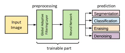
Figure 1: Diagram of the proposed method. Global Adaptive Filtering Layer is trained together with the weights of the main neural network until the prediction is maximized in a given CV task.

Data preprocessing is an essential part of any CV algorithm [39], primarily done in the image space [8]. Proposing the same in the Fourier space, we want to dismiss the meaningless features associated with spectral frequencies brought to the scene by the image acquisition systems (an ultrasound machine or a photo camera, in our case). As such, the method we look for belongs to the class of minimum features inductive bias algorithms [13]. The desired ‘smart’ spectral preprocessing method should automatically distill the meaningful frequencies, being aware of the entire model and ‘adapting’ to the entire dataset.

We propose the concept of such a globally adaptive neural layer (see Fig. 1), which could be trained together with a model of interest to solve a given CV problem. By placing this layer in front of the baseline model, the algorithm should automatically select the weights for the frequency components of all images sent in as the input to carry out filtering with one purpose only: improve whatever the main architecture attempts to do.

Theoretically [5, 21, 7], while performing the Fourier transform, it is possible to move from the frequency domain to the spatial one (and vice versa) without a loss of information. The Fourier transform has the property of linearity, preserving the accuracy of signal approximation (Parseval’s theorem [5]), which is valid when the signal is represented using discrete vectors. Define the Fourier transform as

$$\mathcal{F}I(\mathtt{u},\mathtt{v})=\sum\limits_{\mathtt{x}=0}^{n-1}\sum\limits_{\mathtt{y}=0}^{m-1}\frac{I(\mathtt{x},\mathtt{y})}{nm}\exp\left\{-\frac{2\pi i\mathtt{x}\mathtt{u}}{n}-\frac{2\pi i\mathtt{y}\mathtt{v}}{m}\right\},$$

where $I$ is the original image (spatial description) of size $n\times m$, and $\mathcal{F}I$ is the frequency domain image. If the image has multiple channels, we transform each channel separately by the same formula.

For the visual analysis of Fourier transform, one usually works with the spectrum, i.e., the coordinate-wise absolute value $|\mathcal{F}I|$, or the energy spectrum $|\mathcal{F}I|^{2}$. To filter image in the frequency domain, we choose to take a function that modifies spectrum $|\mathcal{F}I|$ in a specific way. There is flexibility in designing filtering functions [21]. E.g., one can independently select the frequencies to suppress or enhance; however, due to the wide variety of options and the specifics of each task, it is very difficult to select them manually. In contrast, the proposed design of the filtering layer shown in Fig. 1 is capable of automatically forming a more sophisticated and a task-specific filter .

To approximate an arbitrary nonlinear function that performs the desired filtering, a neural network with just one hidden layer is enough, yielding:

$$|\mathcal{F}I|\leftarrow W_{2}*\sigma{\Bigl{(}W_{1}*|\mathcal{F}I|+B_{1}\Bigr{)}}+B_{2},$$

where $W_{1}$ and $W_{2}$ are the weight matrices with non-negative elements, $B_{1}$ are $B_{2}$ are the bias matrices with non-negative elements, $\sigma(\cdot)$ is some nonlinear activation function, and “$*$” denotes element-wise multiplication. Algorithm 1 describes the complete function of the proposed global adaptive filtering layer.

1:Input: $I$ – Initial image.

2:   $\mathcal{F}$ – Fast Fourier Transform operator.

3:$W_{1}$, $W_{2}$, $B_{1}$, $B_{2}$ = ReLU( $W_{1}$, $W_{2}$, $B_{1}$, $B_{2}$);

4:$F$ = $\mathcal{F}I$;

5:$S$ = $W_{2}*\sigma{\Bigl{(}W_{1}*|F|+B_{1}\Bigr{)}}+B_{2}$;

6:$S$ = $S*F/|F|$;

7:$I^{\prime}$ = $\mathcal{F}^{-1}S$;

8:Output: $I^{\prime}$ – Image after global frequency filtering.

Algorithm 1 Global Adaptive Filtering Layer

Handling small frequency values.

When a base neural network is chosen, our layer is pre-pended to it and, then, evaluated with several variations to experiment with the small values of non-central frequencies. Namely, for the Linear configuration, a simple single layer neural network of Algorithm 1 is used. For the General configuration, the exponential transform was additionally applied:

$$|\mathcal{F}I|\leftarrow\exp{\Bigl{[}W*\log{(1+|\mathcal{F}I|)}\Bigr{]}}-1,$$

where $W$ is the trained weight matrix (non-negative). For the Linear log and the General log configurations, only the log transforms of the spectra were computed. These configurations are designed to ‘boost’ the appearance of the smallest frequency pixel values in the spectrum, where the intensity of a typical central frequency oftentimes ‘overwhelms’ the smaller values on the periphery (see insets in Fig. 2 below to see typical spike-shaped learnt spectra).

Number of parameters.

The complex values of Fourier transform are tackled by the operation $|\mathcal{F}I|$. Yet, the important symmetry property $\mathcal{F}I(n-u,m-v)=\mathcal{F}I(-u,-v)=\mathcal{F}I(u,v)^{*}$ helps to compute the number of parameters added by the adaptive layers. Namely, each matrix of weights is a tensor of size $\bigl{(}C,n,\lfloor{m/2\rfloor}+1\bigr{)}$, where $C$ is the number of channels, $(n,m)$ is the image size. Thus, the number of learnable parameters of the proposed adaptive layer is equal to the number of weight matrices multiplied by the product of the matrix dimensions (as the operations in the frequency space are element-wise).

4 Experiments and Results

In this section, we compare the performance of renowned neural networks with and without the proposed trainable layers. In all four tasks, we always choose the most popular models, common initialization strategies, and only the well-known activation and loss functions. We aim to make the existing network architectures more efficient.

Hyperparameters common to all tasks. All models are trained setting the input size to (256, 256), batch size 4, and using Adam optimizer [20] with learning rate 0.001.

4.1 Datasets

We validate efficiency of our adaptive layer on two medical and on four natural image benchmarks.

The medical benchmarks comprise ultrasonic datasets, popular in medical vision community: Breast Ultrasound Images (BUSI [3], 1578 images of three classes: normal (266), benign (891) and malignant (421) tumors, as well as ground-truth segmentation masks) and Brachial Plexus Ultrasound Images (BPUI [1], 5635 images and masks).

The natural benchmarks were selected to represent well-known datasets of various scales: from the small Caltech Birds (Caltech-UCSD Birds-200-2011 [42], 11,788 images of 200 classes with ground-truth segmentation masks), to medium Dogs vs. Cats ([2], 25k images for binary classification), to large-scale CIFAR-10 ([22], 50k images of 10 classes) and a part of ImageNet (‘Tiny’ ImageNet [24], 110k images of 200 classes).

We considered medical imaging datasets separately because the ultrasound signal is known to have particular frequency bands needed for the optimal image contrast in live imaging [19], making us hypothesize that the filtering effect would be more pronounced in these data. Dataset details and descriptions are given in the Supplementary material.

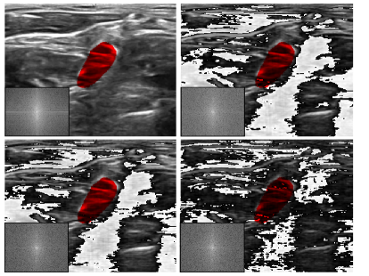
Figure 2: Segmentation Results. Examples of ’learnt’ filters and their effect on the segmentation. Top left: original image and ground-truth mask; top right: Linear filter; bottom left: General filter; bottom right: General log filter. Corresponding ‘learnt’ spectra are shown in the insets in the corner.

4.2 Segmentation

To test the proposed method, three different networks were studied as the base models: U-Net [35], DenseNet [17], and ResNet [15].

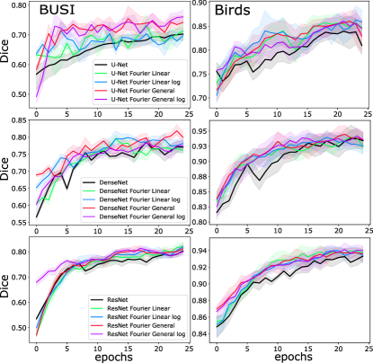
Figure 3: Segmentation Results. Average Dice coefficients on validation sets of different datasets: medical (BUSI) and natural (Birds). Top row: U-Net, middle: DenseNet, bottom: ResNet.

For the learning process, we used the Combined Loss function of Dice and Cross Entropy, weighted as 0.6 and 0.4 respectively. The quality of segmentation is evaluated with the Dice coefficient [29], which, in essence, measures the overlap between the predicted and the ground-truth masks.

The following hyperparameters were used. For U-Net, init_features = 32 (number of parameters in initial convolution), depth = 3 (number of downsteps). For DenseNet (as for densenet-121), init_features = 32, growth_rate = 32 (number of filters to add to each layer), block_config = 6, 12, 24, 16 (number of layers in each pooling block). For ResNet (as for resnet-18), blocks: 2, 2, 2, 2 (number of layers in each pooling block).

Table 1: Segmentation Results. Validation Dice score for different models on medical (BUSI and BPUI) and natural (Caltech Birds) datasets. Red: the worst model, green: the best model.

Model	BUSI	BPUI	Birds
U-Net	0.70	0.59	0.84
+ Fourier Linear	0.72	0.64	0.85
+ Fourier Linear log	0.71	0.64	0.86
+ Fourier General	0.75	0.74	0.86
+ Fourier General log	0.75	0.74	0.86
DenseNet	0.77	0.74	0.94
+ Fourier Linear	0.79	0.77	0.94
+ Fourier Linear log	0.80	0.77	0.94
+ Fourier General	0.81	0.74	0.95
+ Fourier General log	0.77	0.75	0.94
ResNet	0.80	0.71	0.93
+ Fourier Linear	0.81	0.72	0.94
+ Fourier Linear Log	0.81	0.72	0.94
+ Fourier General	0.81	0.74	0.94
+ Fourier General Log	0.81	0.75	0.94

We observe improvement of the segmentation performance in all three base models, as summarized in Figs. 2, 3, and in Table 1. Comprehensive results for each dataset and each model are given in the Supplementary material.

4.3 Classification

To verify the suggested algorithm for the classification problem, a typical Convolutional Neural Network (CNN) with several convolutional blocks and fully-connected layers is used. Namely, the encoder blocks include conv, Batch Normalization, ReLU, Average Pooling, and two fully-connected layers (using init_features = 8 and depth = 4). The training process is similar to the one above, with using the weighted Cross Entropy Loss [16] combined with the $F_{1}$-score evaluation. The results for this task for medical and natural datasets are presented in Fig. 4 and Table 2. Additional natural image classification experiments were performed on large-scale datasets CIFAR-10 and ImageNet, with the results presented in Table 3 and Fig. 6.

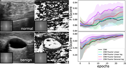
Figure 4: Classification Results: Binary. Left: Initial and filtered images using our layer in General log configuration. Insets show the ‘learnt’ optimal spectra. Right: $F_{1}$-scores on BUSI validation sets (normal vs. benign and benign vs. malignant).

Table 2: Classification Results: Binary. $F_{1}$-scores for different models on BUSI validation set (normal vs. benign and benign vs. malignant classes), and Dogs vs. Cats datasets. Red: the worst model, green: the best model.

Model	BUSI	BUSI	D vs. C
	norm vs. ben	ben vs. mal
CNN	0.88	0.76	0.82
+ Fourier Linear	0.89	0.78	0.83
+ Fourier Linear log	0.89	0.77	0.82
+ Fourier General	0.90	0.76	0.82
+ Fourier General log	0.92	0.77	0.83

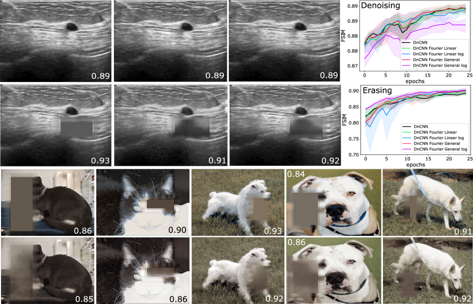
Figure 5: Denoising/Erasing Results. Plots on the right show FSIM metrics for denoising and erasing corruptions of BUSI dataset for different models. First and second row images, left to right: base DnCNN model results, the model with Linear, and with General adaptive filters on BUSI dataset. Third and fourth rows, left to right: base model and model with Linear adaptive filtering layer on the Dogs vs. Cats dataset. Note how addition of Fourier-based layer corrects for the corruptions better (e.g., dog images in fourth vs. third row).

4.4 Denoising and Erasing

For the problem of denoising and erasing, we considered popular model DnCNN [45] as the baseline, the main task of which is to restore the noise, in contrast to the standard feedforward models, which restore the image. To assess the success of denoising and erasing, we used Combined Loss function of MS-SSIM and $L_{1}$ Loss with weights 0.8 and 0.2 respectively [48] along with the FSIM and PSNR metrics [47]. Regular Gaussian noise and rectangular erasing corruptions [49] were introduced to the images, with the consequent image recovery yielding the outcomes summarized in Fig. 5. For the denoising and erasing problems, we used the following hyperparameters: init_features = 64, num_layers = 17 (number of layers).

4.5 Control and large-scale experiments

To gauge the impact of the added layer on the base model precisely, a fine control of the total number of trainable parameters is desirable. Therefore, additional studies were performed for each CV problem, assuring that the number of parameters in base models was either greater or equal of that with the pre-pended adaptive filtering layer (Table 3 and Fig. 6). In this sub-study, all experiments were run using the Linear configurations of the adaptive layer.

Table 3: Control Experiments Results. Comparison between different models for segmentation (Dice score), classification (Accuracy), and Gaussian denoising and erasing corruptions (PSNR). The number of parameters in all experiments is controlled not to exceed the number of parameters in the corresponding base models.

Model	Segmentation		Classification		Denoising	Erasing
	BUSI	Birds	CIFAR-10	Tiny ImageNet	BUSI	BUSI
Base model	0.64	0.86	0.782	0.345	30.69	23.28
+ Fourier Linear	0.69	0.86	0.792	0.348	30.42	22.91
+ Fourier Linear log	0.70	0.86	0.796	0.336	30.66	23.92

Figure 6: Control and Large-Scale Experiments. Metrics on validation sets for different models. Top row: Dice score for segmentation problem on medical (BUSI, left) and natural (Caltech Birds, right) datasets. Middle row: Prediction accuracy for classification problem on CIFAR-10 (left) and Tiny ImageNet (right) datasets. Bottom row: PSNR metric for Gaussian denoising (left) and erasing corruption (right) problems on BUSI dataset.

For the segmentation task, U-Net with init_features = 32 was compared against U-Net with init_features = 16 along with adaptive layer for BUSI (with image_size = (512, 512), yielding 467,266 parameters in base model vs. 248,994 parameters in ours) and Caltech Birds (with image_size = (256, 256), yielding 467,842 parameters in base model vs. 216,770 parameters in ours) datasets.

For the classification task, ResNet-20 was compared with the same model pre-pended by the adaptive layer for CIFAR-10 (with image_size = (32, 32), yielding 276,026 vs. 274,394 parameters) and Tiny ImageNet (with image_size = (64, 64), yielding 293,080 vs. 286,744 parameters) datasets. For these experiments, SGD optimizer with weight decay of 0.0001, momentum of 0.9, and learning rate 0.1 was used.

For the denoising and erasing tasks, DnCNN with init_features = 32 and num_layers = 20 was compared to itself with init_features = 16 and num_layers = 17 and with the pre-pended adaptive layer for BUSI (with image_size = (512, 512), yielding 168,225 vs. 167,169 parameters).

5 Discussion

Remarkably, in the controlled experiments, we observed that the number of parameters in the base model could be reduced by half; yet, the global adaptive filtering layer allows to ‘catch up’ with the lost parameters and to reach the level of the base models that have twice as many parameters. The result generalize well across different datasets of various scales and across CV tasks. We did not observe a stunning improvement in the denoising problem built around DnCNN model – a result we attribute to the way the noise is handled in the Fourier domain, making our metric choice somewhat sub-optimal. Additional studies are required with the DnCNN to understand the enhancement dynamics; however, the same very model is well improved by our layer when there is a notable corruption (the erasing problem). We can visually confirm that our adaptive configuration denoises and ‘heals’ the corruptions better than the base DnCNN model alone.

Activation Functions.

The activation function used in the general configuration of proposed global filtering layer is a hyperparameter that needs to be selected depending on the problem being solved and the dataset. In the provided algorithm, the function receives a non-negative matrix as input; it is since the frequency with negative weight has no physical interpretation. Therefore, several popular activation functions have been selected and investigated. As can be seen in the results in the Supplementary material, the activation function plays an important role. The average difference between the best and worst activation functions in some cases can lead to about 10% gain by metric. It should be noted that the activation functions Mish and ReLU have shown themselves well on all datasets. So, Mish and ReLU are good for using our algorithm out of the box. Note that all the experiments reported in the main text were carried out using ReLU activation function.

Medical vs. Natural Datasets.

In datasets collected using ultrasound imaging, there are a lot of negative examples (with a zero or an empty mask). Unlike the Caltech Birds dataset, such data require more focus, dedication, and expertise to annotate them with labels. But, as with all human-tagged data, one should expect artefacts and potential errors in the markings: for example, the BPUI data have been annotated by pseudo-experts (people who have been trained and instructed by experts).

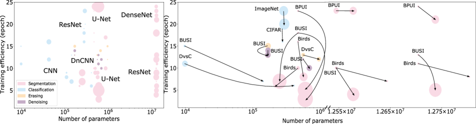
Figure 7: Training efficiency as a function of model complexity for all 88 experiments. The bubble size encodes the gain in the corresponding metrics. Left: all experiments; right: zoomed-in areas. Colours correspond to different types of 4 CV tasks considered. Vertical and left-leaning arrows correspond to 18 control experiments run with precise control of the number of parameters in the models. The arrows indicate the correspondence of pairs (basic model $\to$ the most training-efficient model with the proposed adaptive Fourier layer). Birds: Caltech Birds (2011) dataset; DvsC: Dogs vs. Cats dataset; CIFAR: CIFAR-10 dataset; ImageNet: Tiny ImageNet dataset.

Several important observations and conclusions can be made from the results in the figures herein and from those in the Supplementary material:

• The observed improvement of Dice score on the ultrasound datasets depends on the number of parameters of the base model: the larger the architecture size, the less noticeable the increase in the metric when using the adaptive layer.

• In the natural images dataset, there is a faster convergence of all models when the proposed filtering layer is added, than in any of the base models.

• The proposed log operation applied to the spectra allows for the small pixel values and eliminates fluctuation artefacts otherwise appearing from the truncation.

• Addition of the adaptive filter to the natural images provides “smoother” convergence of the training curves. We believe this trait could be instrumental for accelerating many state-of-the-art models where predicting the behaviour of the model is important; for example, in reinforcement and/or active learning (Fig. 7).

Erasing metric choice.

At the moment, there are a lot of metrics for assessing the quality of denoising of various types. However, there is no universal one that would accurately correspond to the assessment with the naked eye and is well interpreted in all cases [12]. The most suitable for our task was the FSIM metric, which uses the structure of the Fourier components of the image. However, on a large number of examples (including those provided to you in the Fig. 5), it was noticed that the difference in metric between the base model and the model with the proposed trainable layer should have a larger gap, since filling the inside of the cropped rectangle has greater importance than just averaging. Our experiments with other metrics, such as PSNR, present a sound but still sub-optimal alternative.

6 Conclusions

The method proposed in our work proved to be efficient on all datasets and all classical model architectures that we have considered. In all cases, the use of simple adaptive frequency filtering layer has led to faster convergence of the training process than in the case of the stand-alone model, having shown higher segmentation quality both on train and on test samples. A rather important finding is the increase of Dice score for the case of simple U-Net by around 10% when the adaptive global filter is added. This promises an opportunity for the areas, such as medicine, where getting marked data is an acknowledged challenge, causing one to attempt learning on small datasets. In these cases, the use of heavy models with a large number of parameters is one possible solution which frequently leads to a fast overfit; whereas, addition of simple adaptive filtering layers “trims” unnecessary frequencies in the Fourier domain and makes the model learn only the vital frequencies along with the weights of the main neural network. All of this is accomplished while optimizing the targeted advantage function of interest to a particular application (e.g. , Dice score or $F_{1}$-score).

We believe the proposed layer can be a good add-on for a number of powerful modern preprocessing tools, including those that exist in various AutoML pipelines [11]. In fact, there are many recently devised methods of augmentation and data preprocessing (e.g., see [8]) that still await for frequency filtering capability.

The convergence speed of models plays an important role too. Areas, such as ultrasound imaging, entail big amounts of data, the labelling of which takes a lot of time and requires the involvement of highly qualified experts. Due to this, in CV is relevant task of active learning [37], which implies the further retraining of models. Same applies to tasks which entail unsupervised segmentation [4]. Initially, we anticipated that our adaptive layer would improve convergence and quality primarily in the ultrasound data (the echogenic nature of which is known to be prone to high sensitivity to the frequency knobs). But we were surprised to find out the improvement in the natural images as well. This expands the possible areas of application of the proposed approach and opens up a new direction of research of adaptive layers (e.g. ,in more complex multi-layer architectures [10], in generative and image translation models [32], in learnable frequency kernels [23], in iterative anomaly detection models [41], etc.. Lightening of these models via a simple adaptive filtering layer holds potential for a seamless integration in various CV applications.).

7 Acknowledgements

We thank Nazar Buzun for helpful discussions.

Supplemental material

8 Datasets Description

A more exhaustive description of the datasets (Fig. 8) from the main text, follows below.

Figure 8: Examples of BPUI, Caltech Birds (2011), BUSI, Dogs vs. Cats (columns from left to right) datasets associated with the considered computer vision tasks.

We validate efficiency of our adaptive layer on two medical and on four natural image benchmarks.

The ultrasound data is collected by receiving the echo signal reflected from the surfaces of tissues of different density. Depending on the echogenicity (the ability to reflect or transmit ultrasound waves), different types of structures can be distinguished in the scans: hyper-echoic (white regions on the scan), hypo-echoic (gray regions on the scan), or an-echoic (black regions on the scan). For example, the muscles are hypo-echoic with a striated structure, and the nerves are hyper-echoic with the stippled structure.

Natural images represent a separate class of images because they are collected by regular cameras.

Breast Ultrasound Images (BUSI) dataset

contains medical ultrasound images of breast cancer for different female patients, along with the ground truth masks. The data was collected to address the problem of classification, detection, and segmentation of breast cancer, one of the most common causes of death in women worldwide. All images are divided into three classes: normal, benign tumor, and malignant tumor.

Brachial Plexus Ultrasound Images (BPUI) dataset

is intended for the task of segmentation of the anatomical networks, formed by the anterior branches of the four lower cervical nerves and the first thoracic nerve, called the brachial plexus. Localization of the nerve structures on the ultrasound scans is an important step in the clinical practice. The dataset contains both the images with the plexus and without, as well as the ground truth masks.

Caltech Birds (CUB_200_2011) dataset

provides photographs of 200 different bird species, organized by the classes. Annotations, obtained as the medians over the pixels indicated by 5 different users per image, include the bounding boxes and the segmentation labels. Therefore, for the scope of our work, only the main core contours of the annotation labels are referred to as the ground truth masks.

Dogs vs. Cats dataset

consists of a set of 25 thousand images of cats and dogs with a class label. There is a tremendous diversity in the photos (for instance, a wide variety of backgrounds, angles, poses, lighting), causing difficulties for building a proper automatic classification model.

CIFAR-10 dataset

consists of 50,000 images for training and 10,000 images for the test, size $32\times 32$, which are uniformly distributed over 10 classes: airplane, automobile, bird, cat, deer, dog, frog, horse, ship, truck. Each picture includes only one leading instance of a certain class which can be viewed from an unusual point of view.

Tiny ImageNet dataset

has images of 200 different classes (500 in each) with a size of $64\times 64$, as well as 50 validation images for each class.

9 Spectrum and Phase adjustment

Spectrum.

We look for a global filter that will leave only those frequencies that improve the prediction of the base model. A high-pass filter, in which high frequencies are passed and low frequencies are suppressed, enhances edges. While visualizing details with a low-pass filter reduces outliers and contrast, i.e., yielding a smoothing effect. For each task, one needs a specific filter, which is not easy to select manually (Fig. 9). Therefore, we can delegate the task of filter selection to the computer by integrating the appropriate adaptive neural layer for global frequency filtering, which will be trained alongside the main model.

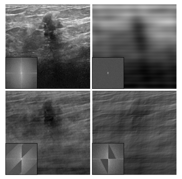
Figure 9: Motivation elaborated. Different frequency filters applied to the initial ultrasonic image (top left) and their Fourier spectra. Notice the effect of high-pass/low-pass components on morphology and texture.

Phase.

We also looked at the phase adjustment, namely, the rotation of each frequency by the trainable angle. The weight matrix remains exactly the same size as in the Linear configuration, but now each weight encodes the angle for which the rotation operator is constructed for each frequency:

$$\begin{bmatrix}f\\ g\end{bmatrix}_{kl}\longleftarrow\mathbf{R}_{w_{kl}}\begin{bmatrix}f\\ g\end{bmatrix}_{kl}=\begin{bmatrix}\cos{w_{kl}}&-\sin{w_{kl}}\\ \sin{w_{kl}}&\cos{w_{kl}}\end{bmatrix}\begin{bmatrix}f\\ g\end{bmatrix}_{kl}$$

where $f_{kl}+jg_{kl}$ is $kl$-th frequency in the Fourier transformed image, $w_{kl}$ is $kl$-th weight in trainable weight matrix $W$. The results of such a learning adjustment can be seen in the Figures 10, 11, 12 for segmentation, classification, denoising and erasing experiments, respectively.

Figure 10: Control and Large-Scale Experiments. Loss functions and Dice coefficients of different models training processes on BUSI (top) and Caltech Birds (bottom) validation sets.

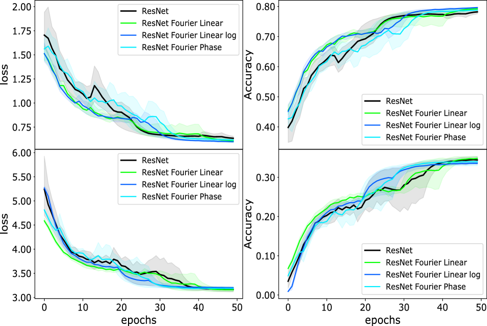
Figure 11: Control and Large-Scale Experiments. Loss functions and Accuracy score of different models training processes on CIFAR-10 (top) and Tiny ImageNet (bottom) validation sets.

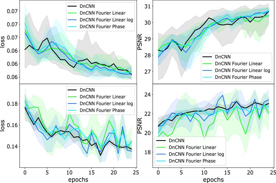
Figure 12: Control and Large-Scale Experiments. Loss functions and PSNR metric of different models training processes for Gaussian denoising (top) and erasing corruption (bottom) problems on BUSI validation set.

10 Segmentation Models Description

Segmentation models have been selected among the following popular ones:

• U-Net - the first successful architecture in biomedical image segmentation, in that rich feature representation combines lower-level image one using skip connections.

• A model with DenseNet encoder, which contains shorter connections between layers close to the input and those close to the output for more accurate and efficient training.

• A model with ResNet encoder, where the layers are reformulated as learning residual functions regarding the layer inputs, instead of learning the unreferenced functions.

11 Activation Functions

The Table 4 contains the results of the study of the activation function influence in the General configuration of the adaptive layer for medical datasets.

Table 4: Validation Dice score for different activation functions on the BUSI and BPUI datasets in the General configuration of the adaptive layer. Red color font corresponds to the worst score, and green font corresponds to the best score.

Activation Function	BUSI			BPUI
	U-Net	DenseNet	ResNet	U-Net	DenseNet	ResNet
Sigmoid	0.70	0.82	0.83	0.68	0.75	0.72
ReLU	0.77	0.84	0.83	0.75	0.77	0.75
ReLU6	0.76	0.83	0.81	0.73	0.76	0.74
Softplus	0.74	0.83	0.82	0.70	0.75	0.74
Tanh	0.75	0.83	0.83	0.73	0.76	0.74
Swish ($\beta=1.0$)	0.78	0.81	0.80	0.74	0.76	0.75
Mish	0.78	0.83	0.82	0.75	0.77	0.75

12 Additional Learning Process Results

As extra information, we provide visualization of learning processes for segmentation (Figures 13, 14, 15, 16, 17, 18, 19, 20), classification (Figures 21, 22), denoising (Fig. 23) and erasing (Figures 24, 25) tasks.

Figure 13: Segmentation. Loss functions and Dice coefficients of different models training processes on BUSI train set.

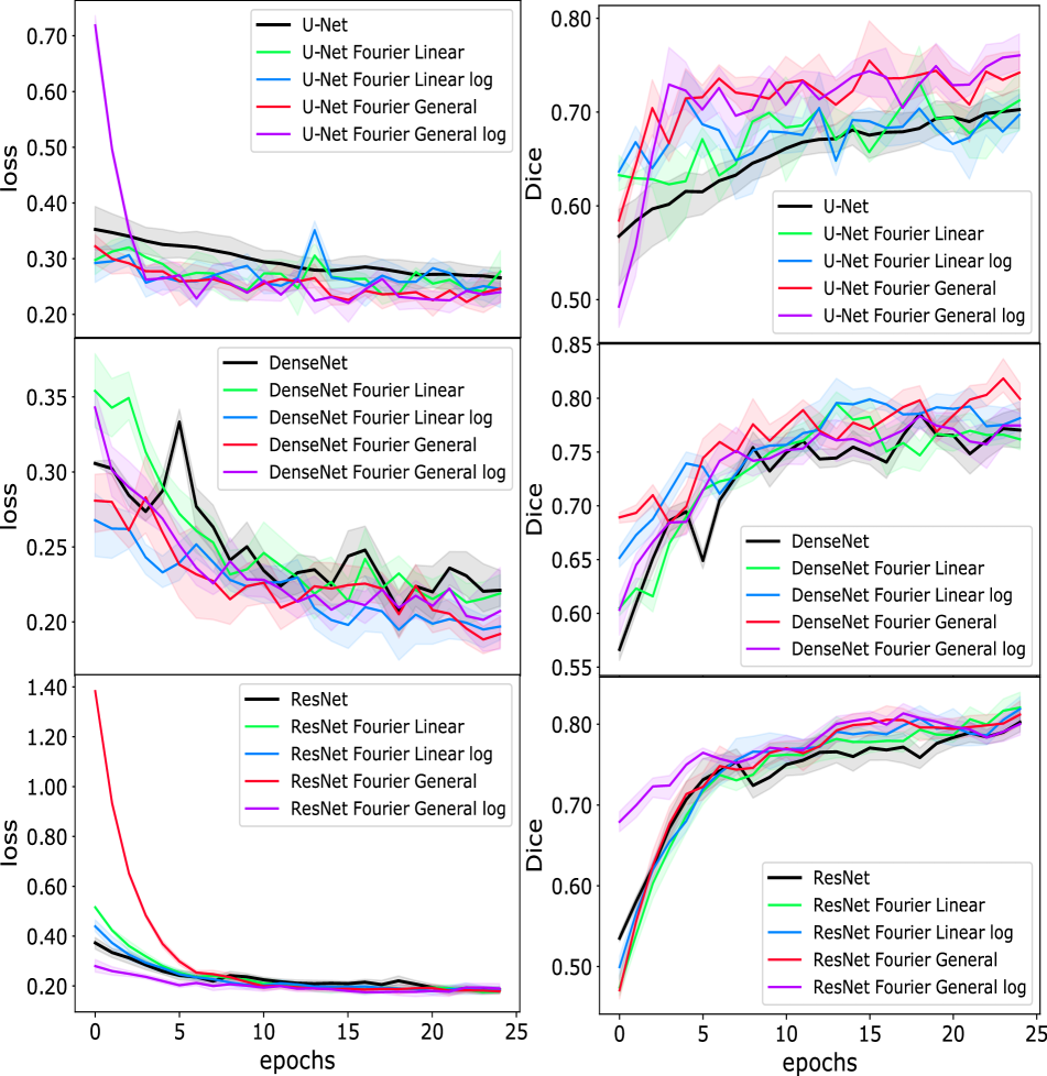
Figure 14: Segmentation. Loss functions and Dice coefficients of different models training processes on BUSI validation set.

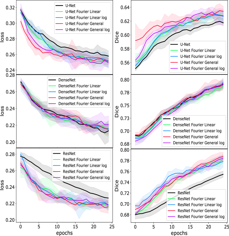
Figure 15: Segmentation. Loss functions and Dice coefficients of different models training processes on BPUI train set.

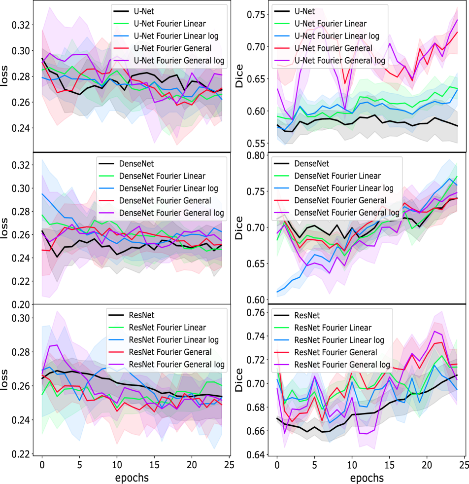
Figure 16: Segmentation. Loss functions and Dice coefficients of different models training processes on BPUI validation set.

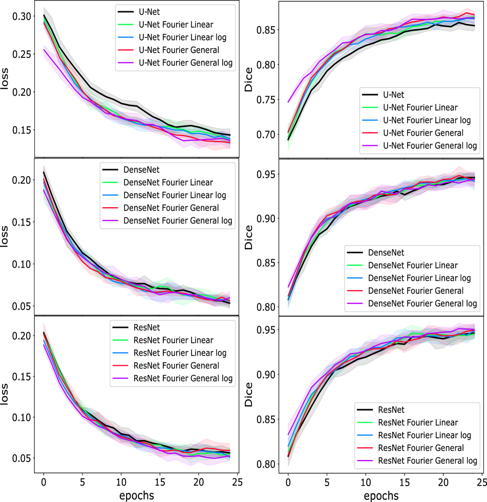
Figure 17: Segmentation. Loss functions and Dice coefficients of different models training processes on Caltech Birds (2011) train set.

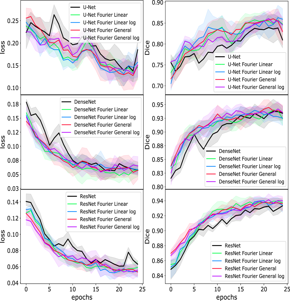
Figure 18: Segmentation. Loss functions and Dice coefficients of different models training processes on Caltech Birds (2011) validation set.

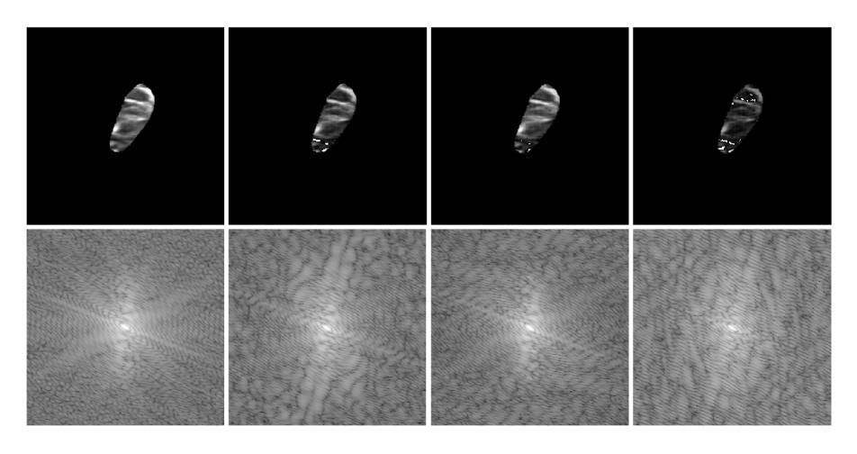
Figure 19: Segmentation. Example of trainable filter application to mask area. Initial image, Linear filter, General filter, General log filter.

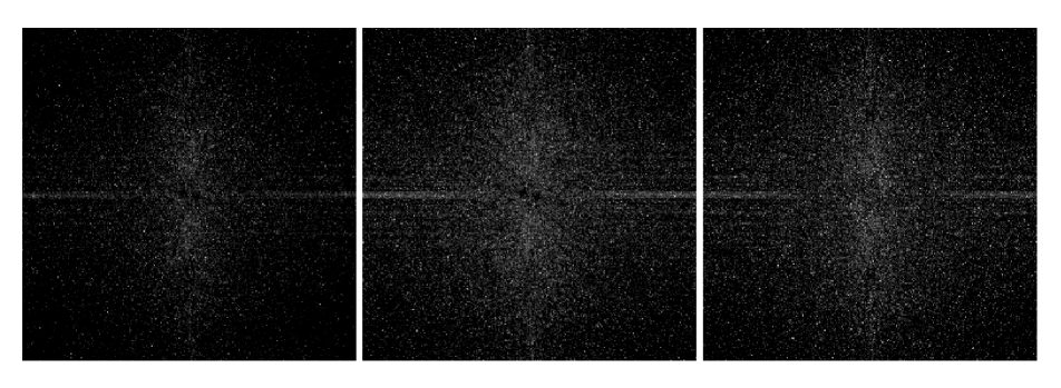
Figure 20: Segmentation. Frequency difference of ‘learnt’ filters (left to right: Linear, General, General log) with the initial spectrum.

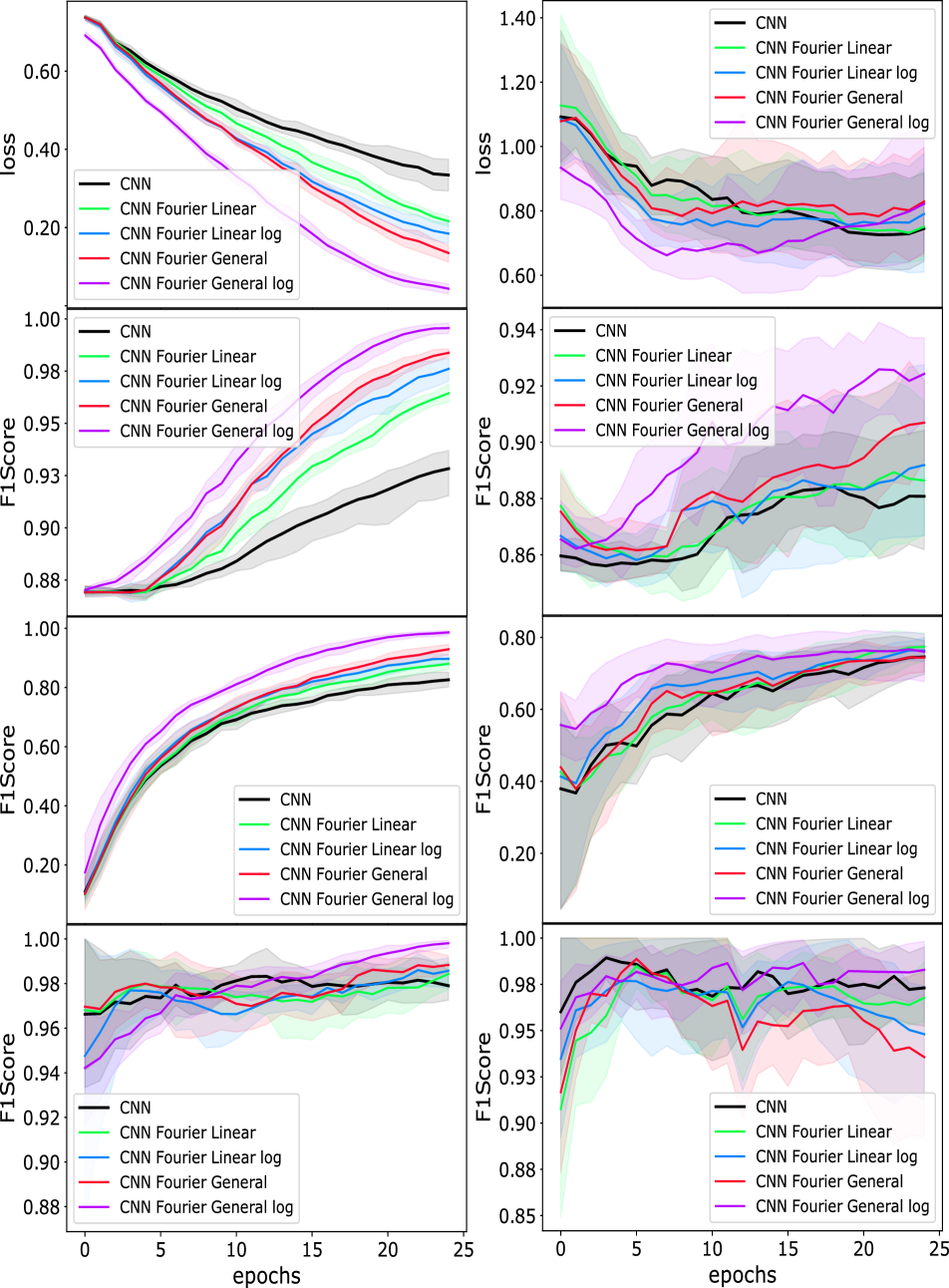
Figure 21: Classification. Loss functions and $F_{1}$-scores of different models training processes on BUSI train (left column) and validation (right column) sets for normal vs. benign, benign vs. malignant and normal vs. malignant class pairs correspondingly.

Figure 22: Classification. Loss functions and $F_{1}$-scores of different models training processes on Dogs vs. Cats train (left column) and validation (right column) sets.

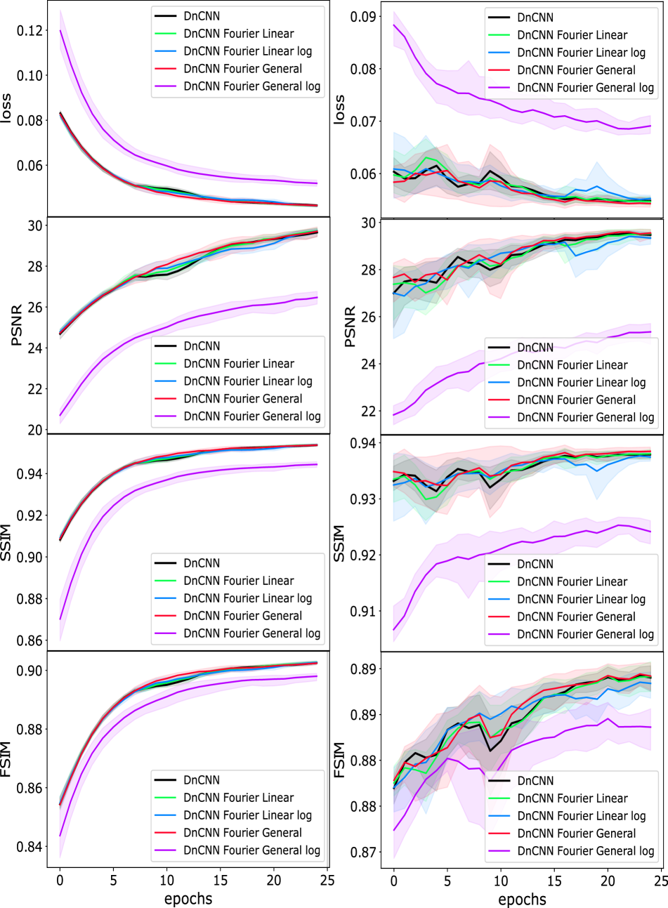
Figure 23: Denoising. Loss functions and PSNR, SSIM, FSIM metrics of different models training processes on BUSI train (left column) and validation (right column) sets.

Figure 24: Erasing. Loss functions and PSNR, SSIM, FSIM metrics of different models training processes on BUSI train (left column) and validation (right column) sets.

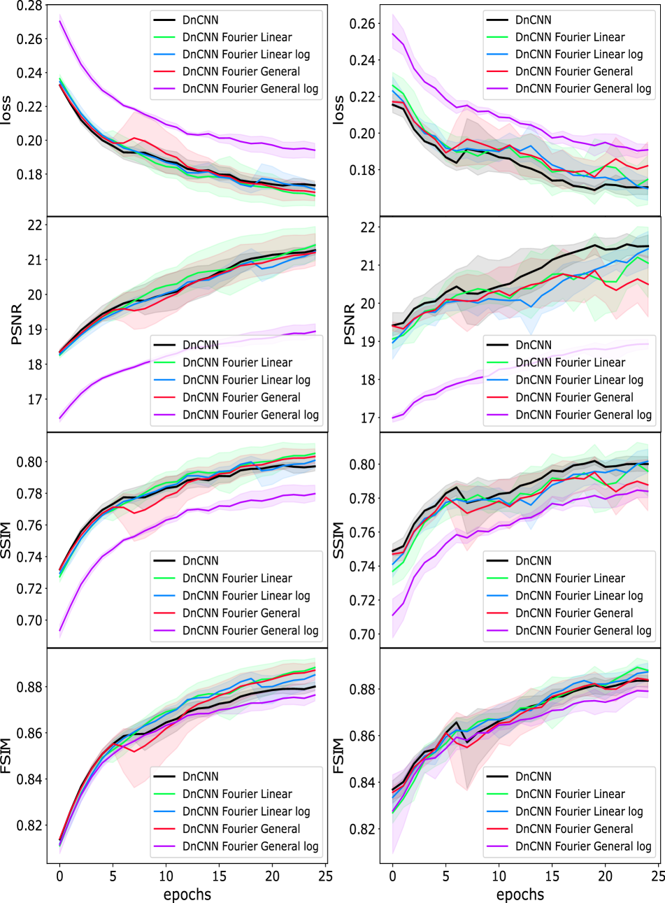
Figure 25: Erasing. Loss functions and PSNR, SSIM, FSIM metrics of different models training processes on Dogs vs. Cats train (left column) and validation (right column) sets.

References

- [1] https://www.kaggle.com/c/ultrasound-nerve-segmentation/data.
- [2] https://www.kaggle.com/c/dogs-vs-cats/data.
- [3] Walid Al-Dhabyani, Mohammed Gomaa, Hussien Khaled, and Aly Fahmy. Dataset of breast ultrasound images. Data in Brief, 28:104863, 11 2019.
- [4] Iaroslav Bespalov, Nazar Buzun, and Dmitry V Dylov. Brulé: Barycenter-regularized unsupervised landmark extraction. arXiv preprint arXiv:2006.11643, 2020.
- [5] J.M. Blackledge. Digital Image Processing: Mathematical and Computational Methods. 11 2005.
- [6] Sing-Tze Bow. Pattern Recognition and Image Preprocessing. Marcel Dekker, Inc., USA, 2nd edition, 2002.
- [7] Steven Brunton and J. Kutz. Data-Driven Science and Engineering: Machine Learning, Dynamical Systems, and Control. 01 2019.
- [8] Alexander Buslaev, Vladimir I. Iglovikov, Eugene Khvedchenya, Alex Parinov, Mikhail Druzhinin, and Alexandr A. Kalinin. Albumentations: Fast and flexible image augmentations. Information, 11(2):125, Feb 2020.
- [9] Vikas Chaudhary and Shahina Bano. Thyroid ultrasound. Indian journal of endocrinology and metabolism, 17:219–27, 03 2013.
- [10] Aritra Chowdhury, Dmitry V Dylov, Qing Li, Michael MacDonald, Dan E Meyer, Michael Marino, and Alberto Santamaria-Pang. Blood vessel characterization using virtual 3d models and convolutional neural networks in fluorescence microscopy. pages 629–632. IEEE, 2017.
- [11] Ekin D. Cubuk, Barret Zoph, Dandelion Mane, Vijay Vasudevan, and Quoc V. Le. Autoaugment: Learning augmentation policies from data. 2019.
- [12] Keyan Ding, Kede Ma, Shiqi Wang, and Eero P. Simoncelli. Comparison of Image Quality Models for Optimization of Image Processing Systems. arXiv e-prints, page arXiv:2005.01338, May 2020.
- [13] Diana F Gordon and Marie Desjardins. Evaluation and Selection of Biases in Machine Learning. Machine Learning, 20(1):5–22, 1995.
- [14] Yanming Guo, Yu Liu, Ard Oerlemans, Songyang Lao, Song Wu, and Michael S. Lew. Deep learning for visual understanding: A review. Neurocomputing, 187:27 – 48, 2016. Recent Developments on Deep Big Vision.
- [15] Kaiming He, Xiangyu Zhang, Shaoqing Ren, and Jian Sun. Deep residual learning for image recognition. CoRR, abs/1512.03385, 2015.
- [16] Yaoshiang Ho and Samuel Wookey. The real-world-weight cross-entropy loss function: Modeling the costs of mislabeling. IEEE Access, PP:1–1, 12 2019.
- [17] Gao Huang, Zhuang Liu, and Kilian Q. Weinberger. Densely connected convolutional networks. CoRR, abs/1608.06993, 2016.
- [18] Huimin Huang, Lanfen Lin, Ruofeng Tong, Hongjie Hu, Zhang Qiaowei, Yutaro Iwamoto, Xian-Hua Han, Yen-Wei Chen, and Jian Wu. Unet 3+: A full-scale connected unet for medical image segmentation. 04 2020.
- [19] Barys Ihnatsenka and Andre Boezaart. Ultrasound: Basic understanding and learning the language. International journal of shoulder surgery, 4:55–62, 07 2010.
- [20] Diederik Kingma and Jimmy Ba. Adam: A method for stochastic optimization. International Conference on Learning Representations, 12 2014.
- [21] Reinhard Klette. Concise Computer Vision: An Introduction into Theory and Algorithms. Springer Publishing Company, Incorporated, 2014.
- [22] A. Krizhevsky and G. Hinton. Learning multiple layers of features from tiny images. Computer Science Department, University of Toronto, Tech. Rep, 1, 01 2009.
- [23] Elizaveta Lazareva, Oleg Rogov, Olga Shegai, Denis Larionov, and Dmitry V Dylov. Learnable hollow kernels for anatomical segmentation. arXiv preprint arXiv:2007.05103, 2020.
- [24] Y. Le and X. Yang. Tiny imagenet visual recognition challenge. 2015.
- [25] Jianghong Li, Liang Chen, and Yuanhu Cai. Dynamic texture segmentation using fourier transform. Modern Applied Science, 3, 08 2009.
- [26] Jinhua Lin, Lin Ma, and Yu Yao. A fourier domain training framework for convolutional neural networks based on the fourier domain pyramid pooling method and fourier domain exponential linear unit. IEEE Access, PP:1–1, 08 2019.
- [27] Pengju Liu, Hongzhi Zhang, Kai Zhang, Liang Lin, and Wangmeng Zuo. Multi-level wavelet-cnn for image restoration. CoRR, abs/1805.07071, 2018.
- [28] Michael T McCann, Kyong Hwan Jin, and Michael Unser. Convolutional neural networks for inverse problems in imaging: A review. IEEE Signal Processing Magazine, 34(6):85–95, 2017.
- [29] Fausto Milletari, Nassir Navab, and Seyed-Ahmad Ahmadi. V-net: Fully convolutional neural networks for volumetric medical image segmentation. 06 2016.
- [30] Ozan Oktay, Jo Schlemper, Loïc Le Folgoc, Matthew C. H. Lee, Mattias P. Heinrich, Kazunari Misawa, Kensaku Mori, Steven G. McDonagh, Nils Y. Hammerla, Bernhard Kainz, Ben Glocker, and Daniel Rueckert. Attention u-net: Learning where to look for the pancreas. CoRR, abs/1804.03999, 2018.
- [31] H. Pratt, B. M. Williams, F. Coenen, and Yalin Zheng. Fcnn: Fourier convolutional neural networks. ECML/PKDD, 2017.
- [32] Denis Prokopenko, Joël Valentin Stadelmann, Heinrich Schulz, Steffen Renisch, and Dmitry V Dylov. Unpaired synthetic image generation in radiology using gans. pages 94–101. Springer, Cham, 2019.
- [33] Waseem Rawat and Zenghui Wang. Deep convolutional neural networks for image classification: A comprehensive review. Neural Computation, 29(9):2352–2449, 2017. PMID: 28599112.
- [34] M. Rhu, N. Gimelshein, J. Clemons, A. Zulfiqar, and S. W. Keckler. vdnn: Virtualized deep neural networks for scalable, memory-efficient neural network design. In 2016 49th Annual IEEE/ACM International Symposium on Microarchitecture (MICRO), pages 1–13, 2016.
- [35] Olaf Ronneberger, Philipp Fischer, and Thomas Brox. U-net: Convolutional networks for biomedical image segmentation. CoRR, abs/1505.04597, 2015.
- [36] Noam Shazeer, Azalia Mirhoseini, Krzysztof Maziarz, Andy Davis, Quoc Le, Geoffrey Hinton, and Jeff Dean. Outrageously large neural networks: The sparsely-gated mixture-of-experts layer, 2017.
- [37] Artem Shelmanov, Vadim Liventsev, Danil Kireev, Nikita Khromov, Alexander Panchenko, Irina Fedulova, and Dmitry V Dylov. Active learning with deep pre-trained models for sequence tagging of clinical and biomedical texts. pages 482–489. IEEE, 2019.
- [38] Junho Song, Young Jun Chai, Hiroo Masuoka, Sun-Won Park, Su-jin Kim, June Choi, Hyoun-Joong Kong, Kyu Eun Lee, Joongseek Lee, Nojun Kwak, Ka Yi, and Akira Miyauchi. Ultrasound image analysis using deep learning algorithm for the diagnosis of thyroid nodules. Medicine, 98:e15133, 04 2019.
- [39] Richard Szeliski. Computer vision algorithms and applications. Springer, London; New York, 2011.
- [40] Matthew Tancik, Pratul Srinivasan, Ben Mildenhall, Sara Fridovich-Keil, Nithin Raghavan, Utkarsh Singhal, Ravi Ramamoorthi, Jonathan Barron, and Ren Ng. Fourier features let networks learn high frequency functions in low dimensional domains. 06 2020.
- [41] Nina Tuluptceva, Bart Bakker, Irina Fedulova, Heinrich Schulz, and Dmitry V Dylov. Anomaly detection with deep perceptual autoencoders. arXiv preprint arXiv:2006.13265, 2020.
- [42] C. Wah, S. Branson, P. Welinder, P. Perona, and S. Belongie. The Caltech-UCSD Birds-200-2011 Dataset. Technical Report CNS-TR-2011-001, California Institute of Technology, 2011.
- [43] Lei Wang, Shujian Yang, Shan Yang, Cheng Zhao, Guangye Tian, Yuxiu Gao, Yongjian Chen, and Yun Lu. Automatic thyroid nodule recognition and diagnosis in ultrasound imaging with the yolov2 neural network. World Journal of Surgical Oncology, 17, 12 2019.
- [44] Yanchao Yang and Stefano Soatto. Fda: Fourier domain adaptation for semantic segmentation. 04 2020.
- [45] Kai Zhang, Wangmeng Zuo, Yunjin Chen, Deyu Meng, and Lei Zhang. Beyond a gaussian denoiser: Residual learning of deep cnn for image denoising. IEEE Transactions on Image Processing, PP, 08 2016.
- [46] Kai Zhang, Wangmeng Zuo, Yunjin Chen, Deyu Meng, and Lei Zhang. Beyond a Gaussian denoiser: Residual learning of deep CNN for image denoising. IEEE Transactions on Image Processing, 26(7):3142–3155, 2017.
- [47] Lin Zhang, Lei Zhang, Xuanqin Mou, and David Zhang. Fsim: A feature similarity index for image quality assessment. Image Processing, IEEE Transactions on, 20:2378 – 2386, 09 2011.
- [48] Hang Zhao, Orazio Gallo, Iuri Frosio, and Jan Kautz. Loss functions for image restoration with neural networks. IEEE Transactions on Computational Imaging, PP:1–1, 12 2016.
- [49] Zhun Zhong, Liang Zheng, Guoliang Kang, Shaozi Li, and Yi Yang. Random erasing data augmentation. Proceedings of the AAAI Conference on Artificial Intelligence, 34, 08 2017.
- [50] Zongwei Zhou, Md Mahfuzur Rahman Siddiquee, Nima Tajbakhsh, and Jianming Liang. Unet++: A nested u-net architecture for medical image segmentation. CoRR, abs/1807.10165, 2018.
- [51] Z. Zhou, M. M. R. Siddiquee, N. Tajbakhsh, and J. Liang. Unet++: Redesigning skip connections to exploit multiscale features in image segmentation. IEEE Transactions on Medical Imaging, 39(6):1856–1867, 2020.
- [52] Wangmeng Zuo, Kai Zhang, and Lei Zhang. Convolutional neural networks for image denoising and restoration. Denoising of Photographic Images and Video: Fundamentals, Open Challenges and New Trends, pages 93–123, 2018.