The relative orientation between the magnetic field and gas density structures in non-gravitating turbulent media

Abstract

Magnetic fields are a dynamically important agent for regulating structure formation in the interstellar medium. The study of the relative orientation between the local magnetic field and gas (column-) density gradient has become a powerful tool to analyse the magnetic field’s impact on the dense gas formation in the Galaxy. In this study, we perform numerical simulations of a non-gravitating, isothermal gas, where the turbulence is driven either solenoidally or compressively. We find that only simulations with an initially strong magnetic field (plasma-$\beta<1$) show a change in the preferential orientation between the magnetic field and isodensity contours, from mostly parallel at low densities to mostly perpendicular at higher densities. Hence, compressive turbulence alone is not capable of inducing the transition observed towards nearby molecular clouds. At the same high initial magnetisation, we find that solenoidal modes produce a sharper transition in the relative orientation with increasing density than compressive modes. We further study the time evolution of the relative orientation and find that it remains unchanged by the turbulent forcing after one dynamical timescale.

1 Introduction

Magnetic fields are an essential component of the interstellar medium (ISM, Ferrière, 2001; Crutcher, 2012; Klessen & Glover, 2016). They play an important role in shaping the interstellar gas in and around star-forming clouds, by favouring the formation of filamentary structures and reducing the number of overdensities that can form new stars (see Hennebelle & Inutsuka, 2019; Pattle & Fissel, 2019, for a recent review). However, its exact influence on the cycle of matter in the ISM remains to be better understood.

Observations indicate that the magnetic energy density is in rough equipartition with the other energy densities in the local ISM (Heiles & Crutcher, 2005; Beck, 2015). Gas motions are unaffected when they propagate parallel to the mean direction of the field ($B_{0}$), but strongly inhibited by the magnetic pressure when they propagate normal to $B_{0}$ (Field, 1965). Consequently, the accumulation of gas that precedes the formation of molecular clouds (MCs) is most effective only if the perturbations propagate almost parallel to $B_{0}$ (Hennebelle & Pérault, 2000; Hartmann et al., 2001; Körtgen & Banerjee, 2015; Körtgen et al., 2018). This implies that magnetic fields are a source of asymmetry in the accumulation of interstellar gas from the diffuse ISM.

Such an asymmetry in the distribution of the over-densities in the ISM has been observed toward MCs in the relative orientation between the gas column densities and the plane-of-the-sky magnetic field orientation, inferred from the dust polarised emission observations (Planck Collaboration XXXV, 2016; Fissel et al., 2019; Soler, 2019). Using assumptions on the mapping of the gravitational potential by the distribution of submillimeter emission, Koch et al. (2012) use this asymmetry to infer the local magnetic field strength and its relative importance to other forces in the analysis of SMA polarisation data.

The study of numerical simulations of magnetohydrodynamic (MHD) turbulence in MCs reveals that the relative orientation between density structures ($\rho$) and the magnetic field $\vec{B}$ is related to the magnetisation of the gas (Soler et al., 2013). Isothermal simulations of turbulent MCs show that when the kinetic energy density is larger than the magnetic energy density, $\rho$ structures are aligned to $\vec{B}$ across all $\rho$ values. In contrast, if the magnetisation is high, the $\rho$ structures change orientation from mostly parallel to mostly perpendicular with increasing $\rho$. This result has also been found in simulations of dense core formation in colliding flows (Chen et al., 2016) and, more recently, in MCs selected from 1-kpc-scale multiphase numerical simulations (Seifried et al., 2020).

There are several explanations for the origin of this transition from parallel to perpendicular orientation with increasing density. Chen et al. (2016) argue that the transition happens once the flow becomes super-Alfvénic due to gravitational collapse. More recently, Seifried et al. (2020) found that the change in relative orientation correlates well with the regime, where the gas becomes magnetically supercritical. These two findings are quite similar since the gas becomes gravitationally unstable and magnetically supercritical at roughly the same column density (Vázquez-Semadeni et al., 2011).

Soler & Hennebelle (2017a) developed a theory to describe the evolution of the angle between the magnetic field and the gas structures. They showed that a perpendicular arrangement of magnetic fields and gas structures is a consequence of gravitational collapse or, more generally, converging gas motions. Other interpretations, such as those presented in Hu et al. (2019), assign the anisotropies predicted by the theory of interstellar MHD turbulence as the source of the observed relative orientation between $\rho$ structures and $\vec{B}$ (Goldreich & Sridhar, 1995).

In this work, we investigate the role turbulence plays in setting the relative orientation between the density structures and the magnetic field, mainly focusing on the role of compressive and solenoidal modes. For this purpose, we analyse a set of numerical simulations of driven MHD turbulence in an isothermal gas without an external gravitational potential and self-gravity. Using this numerical experiment, we aim to identify to what extent the observed trends in relative orientation between $\rho$ and $\vec{B}$ is explained by the influence of the different modes of turbulence in the ISM.

This paper is organised as follows. Sec. 2 briefly reviews the basic methodology behind the analysis presented below. Sec. 3 describes the used numerical code as well as the initial conditions for this study. Finally, in Sec. 4, we present and discuss our findings. This study is closed with a summary of our main findings in Sec. 5.

2 Methodology

One method for quantifying the orientation of the density structures is the characterisation through its gradient, which relies on the fact that the density gradients ($\nabla\rho$) are normal to the iso-density contours (Soler et al., 2013). This method has the advantage of providing a direct connection to quantities in the MHD equations. Using this connection, Soler & Hennebelle (2017a) derived the time evolution of the orientation between the magnetic field and the gas density gradient (denoted by the angle $\phi$), which is

$$\frac{\mathrm{dcos}\phi}{\mathrm{d}t}=C+\left(A_{1}+A_{23}\right)\mathrm{cos}\phi,$$ (1)

where the terms are

$$C=-\frac{\partial_{\mathrm{i}}\left(\partial_{\mathrm{j}}v_{\mathrm{j}}\right)}{\left(R_{\mathrm{k}}R_{\mathrm{k}}\right)^{1/2}}b_{\mathrm{i}},$$ (2)

$$A_{1}=\frac{\partial_{\mathrm{i}}\left(\partial_{\mathrm{j}}v_{\mathrm{j}}\right)}{\left(R_{\mathrm{k}}R_{\mathrm{k}}\right)^{1/2}}r_{\mathrm{i}},$$ (3)

$$A_{23}=\frac{1}{2}\left(\partial_{\mathrm{i}}v_{\mathrm{j}}+\partial_{\mathrm{j}}v_{\mathrm{i}}\right)\left[r_{\mathrm{i}}r_{\mathrm{j}}-b_{\mathrm{i}}b_{\mathrm{j}}\right].$$ (4)

Here, $v_{i}$ denotes the fluid velocity,

$$r_{i}\equiv\frac{R_{i}}{\left(R_{k}R_{k}\right)^{1/2}},$$ (5)

with $R_{i}\equiv\partial_{\mathrm{i}}\log\rho$, and

$$b_{i}\equiv\frac{B_{i}}{\left(B_{k}B_{k}\right)^{1/2}},$$ (6)

which are the unit vectors of the gradient of the (logarithmic) density and the magnetic field, respectively. These terms highlight the crucial role of converging and diverging gas motions, represented by the diagonal elements of the shear tensor, $\partial_{\mathrm{i}}v_{\mathrm{j}}$, and their link to the directions of the magnetic field and density gradients. Thus, in general, any process that leads to a spatial change in the velocity field can induce a transition in the relative orientation between the magnetic field and gas density structures. We note that, as discussed in Seifried et al. (2020), any coefficient in Eq. (1) can be responsible for a change in relative orientation. However, in standard scenarios that are not related to strong shocks, the terms related to $\partial_{\mathrm{i}}\left(\partial_{\mathrm{j}}v_{\mathrm{j}}\right)$ tend to be negligible. That leaves the term $A_{23}$, which is related to the velocity strain tensor and the symmetric tensors, as the dominant term in Eq. (1).

3 Numerical simulations

3.1 Initial conditions

We set a cubic box with edge length $L=10\,\mathrm{pc}$. The domain is filled with gas with initial number density $n_{\mathrm{init}}=536\,\mathrm{cm}^{-3}$, which gives a total mass of $M_{\mathrm{tot}}\sim 3\times 10^{4}\,\mathrm{M}_{\odot}$. The gas is isothermal at a temperature of $T=11\,\mathrm{K}$. We use a mean molecular weight $\mu_{\mathrm{mol}}=2.4$, both typical for dense molecular gas. The sound speed associated with this temperature is $c_{\mathrm{s}}=0.2\,\mathrm{km/s}$. These conditions are similar to those studied in Soler et al. (2013).

Since we are interested in the relative orientation of the magnetic field with respect to the density gradient, we set up an initially homogeneous magnetic field $\textbf{B}=B_{0}\hat{\textbf{x}}$, where the field strength $B_{0}$ is calculated from the initial ratio of thermal to magnetic pressure

$$\beta=\frac{P_{\mathrm{th}}}{P_{\mathrm{b}}}=\frac{nk_{\mathrm{B}}T}{B_{0}^{2}/8\pi},$$ (7)

where $k_{\mathrm{B}}$ is Boltzmann’s constant. The turbulence in the domain is driven by an Ornstein-Uhlenbeck process with peak wavenumber $k=2$, which corresponds to half the box size, i.e. $L/2=5\,\mathrm{pc}$ (see e.g. Federrath et al., 2008, 2009, 2010). The contribution from solenoidal or compressive modes is determined by the parameter $\zeta_{\mathrm{d}}$, which enters the projection tensor

$$\mathcal{P}_{\mathrm{ij}}=\zeta_{\mathrm{d}}\left(\delta_{\mathrm{ij}}+\frac{k_{\mathrm{i}}k_{\mathrm{j}}}{\left|k\right|^{2}}\right)+\left(1-\zeta_{\mathrm{d}}\right)\frac{k_{\mathrm{i}}k_{\mathrm{j}}}{\left|k\right|^{2}}.$$ (8)

We choose only the two extreme cases of purely solenoidal driving with $\zeta_{\mathrm{d}}=1$ or purely compressive driving with $\zeta_{\mathrm{d}}=0$. The amplitude of the turbulence forcing term is adjusted in such way that the sonic Mach number in the quasi-stationary state is $\mathcal{M}_{\mathrm{s}}\sim 7.5$. An overview of the initial conditions is given in Tab. 1.

Table 1: List of performed simulations. $\beta$ denotes the initial ratio of thermal to magnetic pressure and the sonic and alfvénic Mach numbers depict the ratio of kinetic to thermal and kinetic to magnetic energy, respectively.

Run name	$\beta$	$\mathcal{M}_{\mathrm{sonic}}$	$\mathcal{M}_{\mathrm{alfvenic}}$	Driving
B10com	10	7.5	16.7	compressive
B10sol	10	7.5	16.7	solenoidal
B1com	1	7.5	5.3	compressive
B1sol	1	7.5	5.3	solenoidal
B0.01com	0.01	7.5	0.5	compressive
B0.01sol	0.01	7.5	0.5	solenoidal

3.2 Numerics

The simulations were performed using the Eulerian finite volume code flash (version 4.6.1, Dubey et al., 2008). During each timestep, flash solves the equations of ideal magnetohydrodynamics using a positive-definite 5-wave Riemann solver (Bouchut et al., 2009; Waagan et al., 2011). Periodic boundary conditions are applied at all domain walls. The root grid is at a resolution of $64^{3}$ and we allow for localised adaptive refinement up to an effective resolution of $512^{3}$. Despite the lack of self-gravity of the gas, the grid is adaptively refined once the local Jeans-length, $\lambda_{\mathrm{J}}$, is resolved by less than eight cells. In addition, de-refinement is applied to regions, where $\lambda_{\mathrm{J}}$ is resolved by more than 16 grid cells.

4 Results

We commence with analysing the relative orientation of the magnetic field and the density gradient. In what follows and not otherwise noted, all data are analysed at 1.5 turn-over times, i.e. in a state in which the turbulent fluctuations can be thought of as in steady-state.

4.1 Overview of the simulation scenarios

We present in Fig. 1 surface density maps for the runs B0.01com, B0.01sol and B1sol. The projection along two different axes reveals pronounced differences. The density structure varies for different driving. The case of compressive driving shows a few regions of enhanced density with the major axis primarily perpendicular to the background magnetic field. The density contrast vanishes almost completely after projection along the background magnetic field. We also note the different morphology of the magnetic field. Solenoidal turbulence driving results in many more substructure, which closely resemble striations, such as those described in Tritsis & Tassis (2016); Chen et al. (2017); Beattie & Federrath (2020). These striations are more pronounced in the case with small plasma-$\beta$, since here the magnetic field is strong enough to guide the flow of gas. This can also be inferred from the magnetic field morphology. While for the low-$\beta$ scenarios, the initial field direction is retained, it is largely disturbed in the $\beta=1$ case. However, the initial magnetic field direction is still dominant.

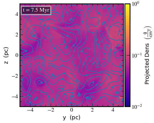
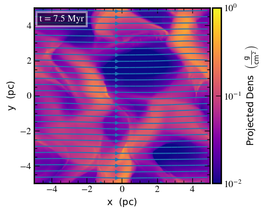
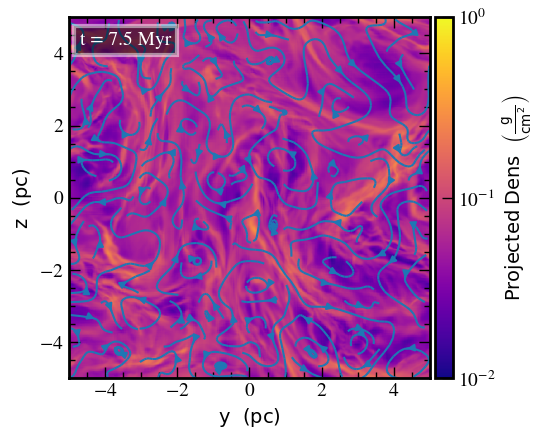
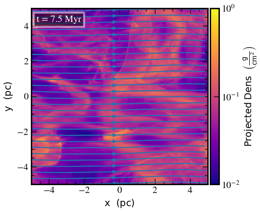
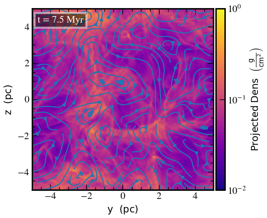
Figure 1: Surface density maps at $t=1.5\,t_{d}$ along the x-direction (i.e. parallel to the initial magnetic field direction, left) and the z-direction (perpendicular to the initial field direction, right) for the runs B0.01com (top), B0.01sol (middle) and B1sol (bottom).

4.2 The relative orientation parameter

We quantify the relative orientation by using the histogram of relative orientation (HRO) shape parameter, a quantity introduced in Soler et al. (2013) and defined as

$$\zeta_{\mathrm{HRO}}\equiv\frac{A_{\perp}-A_{||}}{A_{\perp}+A_{||}},$$ (9)

where $A_{||}$ and $A_{\perp}$ correspond to the counts in the histogram of $\cos\phi$ in the ranges that represent parallel or perpendicular alignment of $\nabla\rho$ and $\vec{B}$. Following the ranges introduced in Soler et al. (2013) and Seifried et al. (2020), we have used $|\cos\phi|<0.25$ for $A_{\perp}$ and $|\cos\phi|>0.75$ for $A_{\parallel}$. The definition of the histogram in terms of $\cos\phi$ acknowledges the fact that, in 3D, the distribution of pairs of randomly oriented vectors is flat in terms of $\cos\phi$ and not in $\phi$. Given the aforementioned definitions, $\zeta_{\mathrm{HRO}}$ $>$ $0$ if the density structures are mostly parallel to the magnetic field (or $\nabla\rho\perp\underline{B}$) and $\zeta_{\mathrm{HRO}}$ $<$ $0$ if the density structures are mostly perpendicular to the magnetic field ($\nabla\rho\parallel\underline{B}$). A homogeneous distribution of relative orientation angles would correspond to $\zeta_{\mathrm{HRO}}$ $\approx$ $0$. We note that more sophisticated methods based on circular statistics have been introduced to characterise the relative orientations in 2D, for example in Jow et al. (2018) and Soler (2019), but its implementation in 3D distributions of angles is still work in progress.
We show $\zeta_{\mathrm{HRO}}$ in multiple bins of gas number density $n$ in Fig. 2. Two main features are observed. First, the values of $\zeta_{\mathrm{HRO}}$ $\approx$ $1$ across $n$ for the weakly magnetised scenarios with $\beta=\left\{1,10\right\}$. This is expected since the magnetic field is sub-dominant in these situations and dragged along with the flow of gas. Therefore, it imposes no asymmetry to the fluid flow. More importantly, there are only minor differences between solenoidally and compressively driven turbulence cases. This means that compressive driving of the turbulence alone, i.e. due to stellar feedback, is not enough to induce a change in relative orientation. In agreement with previous studies of magnetised (and self-gravitating) media (Soler et al., 2013; Soler & Hennebelle, 2017a; Seifried et al., 2020), a dynamically dominant magnetic field must be present.
Second, the decrease of $\zeta_{\mathrm{HRO}}$ with density for the smallest values of $\beta$. This behaviour is typical in such scenarios, since here the magnetic field is strong enough to guide the gas flow. This leads to compression of gas along the field lines and a subsequent build-up of a density gradient parallel to the field. Among the two cases, the one with compressive turbulence shows the earlier decrease of $\zeta_{\mathrm{HRO}}$. This is due to the naturally enhanced divergence of the velocity field, which is zero by definition in the solenoidal case. However, the magnetic and density gradient fields show a tendency for almost no preferred orientation ($\zeta_{\mathrm{HRO}}\approx 0$) after it has started to decrease. There is even a slight re-increase observed at around $\mathrm{log}\left(n\right)\sim 4.4$, before $\zeta_{\mathrm{HRO}}$ transitions towards negative values. The fact that the solenoidally driven case shows a decreasing $\zeta_{\mathrm{HRO}}$ as well is due to the non-linear conversion of solenoidal to compressive modes in the velocity field (Konstandin et al., 2012). However, as this conversion is only efficient enough in the denser gas the start of the decrease naturally appears at higher densities. This effect can be associated with smaller scales that are not influenced by the driving on large scales.
In summary, the strongest magnetisation yields the expected transition from preferentially perpendicular to parallel alignment. When considering the relative orientation at the highest densities ($n$ $>$ $10^{4}$ cm^-3), the relative orientation is the same for the solenoidal and compressive forcing and seems to solely depend on the magnetisation. At lower densities ($10^{2}$ $<$ $n$ $<$ $10^{4}$ cm^-3), there appears some difference between the solenoidal and compressive forcing.

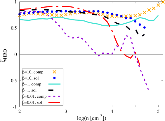
Figure 2: The HRO shape parameter as a function of number density for the different simulations. While the weakly magnetised scenarios show no change in relative orientation, the highly magnetised cases indicate a transition from preferentially perpendicular to parallel alignment (in terms of the density gradient). Note further that the decrease in the shape parameter occurs at smaller densities for the compressive case, although there appears some density regime of no preferred orientation.

4.3 What determines the change in relative orientation?

The form of Eq. (1), provided in Sec. 2, indicates that, if $A_{1}+A_{23}\equiv A>C$, the evolution of the relative orientation depends on the sign of the $A$-coefficient and thus on the relative importance of the change in velocity divergence and the strain in the velocity field (Soler & Hennebelle, 2017a). The resulting density-dependence of $A$ and $C$ is shown in Fig. 3. At the lowest densities, the $A$-term is negative, which indicates a transition towards $\mathrm{cos}\,\phi\rightarrow 0$ according to Eq. (1), as long as $C$ is small. Major deviations in the evolution, however, start to appear already from $\mathrm{log}\left(n\right)\sim 2.5$ on. These deviations are furthermore not only dependent on the magnetisation of the gas, but also depend on the way the turbulence is driven. While the $A$-term in the scenarios B10sol and B1sol becomes even more negative with density, the corresponding terms in the runs with compressive turbulence stay almost constant, with a slight increase towards $A\sim 0$ at the highest densities. In contrast, the two strongly magnetised cases with $\beta=0.01$ show a transition from $A<0$ to $A>0$. As predicted by Soler & Hennebelle (2017a), a transition to $\zeta_{\mathrm{HRO}}<0$ is achieved as soon as the $A$-term changes sign. The change in sign in our case is accompanied by a decrease of $\zeta_{\mathrm{HRO}}$, rather than a transition to below zero. The density regime where $\zeta_{\mathrm{HRO}}\sim 0$ for scenario B0.01com, which indicates no preferred orientation, is described by $A\sim 0$ and thus $C>A$ (see Fig. 3, bottom panel). The corresponding simulation with solenoidal forcing crosses the zero-point line at slightly higher densities. Both strongly magnetised runs then show a sharply increasing $A$ as a function of density.
To sum up, the density dependence of the $A$-term is controlled by the magnetisation of the gas in terms of $A$ transitioning from negative to positive values. On the other hand, for equipartition or very weak fields ($\beta=1$ or $\beta=10$), the evolution appears more likely to be controlled by the type of turbulent forcing. For solenoidal forcing, $A$ becomes more negative, while for compressive forcing it stays rather constant or shows a shallow positive slope as a function of density.

Figure 3: Density dependence of the coefficients entering Eq. (1). Top: Average of the sum of the A-terms. Bottom: The ratio of the average C-term and the total A-term.

4.4 Fluid strain or projected divergence?

Above it was shown that $A>C$ in most cases. Here, we discuss which part of $A$ is responsible for the transition from $A<0$ to $A>0$ and thus for a change in relative orientation from preferentially perpendicular alignment to almost parallel alignment.
Fig. 4 shows the density dependence of each individual, averaged coefficient of Eq. (1). At low densities, the $A$–coefficients are both negative. For the weakly magnetised cases with compressive driving they stay almost constant as a function of density. Generally, the $A_{23}$–term is larger in magnitude at the highest densities, indicating that here the shear in the flow dominates. Note that the $A_{1}$–term transitions to positive values for B1com, but does not become dominant. The corresponding solenoidal cases show no transition to positive values, but instead a further decrease of the $A_{23}$–term.
As stated above, only the runs with initial $\beta=0.01$ transition towards a preferentially parallel alignment. This is due to the fact that $A>C$ and that $A$ becomes positive at some density. The earlier change in relative orientation for the compressive case matches well with the earlier transition of the $A$–coefficient. To be more precise, it is the transition of the $A_{1}$–term and the subsequent dominance of it. The respective $A_{23}$–term becomes positive at almost an order of magnitude higher densities. The behaviour of the individual $A$–terms implies that the gas undergoes strong shocks and that these shocks are more dominant than shear in the fluid flow. In contrast, this large difference in density is not observed for the solenoidal scenario, because here the overall magnitude of the velocity divergence is small. In agreement with Seifried et al. (2020), the coefficients responsible for the change in relative orientation might depend on the specific physical conditions. This is further illustrated by the evolution of $\zeta_{\mathrm{HRO}}$ for the run B0.01com. $\zeta_{\mathrm{HRO}}$ reaches a value of zero, but does not proceed to negative values. Instead, it increases again, before it finally decreases to negative values. As can be seen in Fig. 4, the coefficient $C$ takes non-zero values and does become non-negligible at $n>10^{4}\,\mathrm{cm}^{-3}$. It thus starts to impact the evolution up to the point where $A_{1}$ becomes completely dominant.
In summary, the presented figures reveal that the behaviour of the flow field in a strongly magnetised medium is vital for the details of the change in relative orientation.

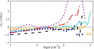
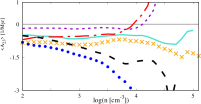
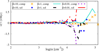
Figure 4: Density dependence of the various individual coefficients, which control the rate of change of the relative orientation. We note that we only show the average values here and that the uncertainty can be large (Seifried et al., 2020). Please note the different scaling of the y–axes.

4.5 Time evolution of the HRO parameter

Here, we investigate the time evolution of the relative orientation parameter. For this, we show in Fig. 5 the shape parameter for times between one and 1.5 dynamical times. Usually, the turbulence is expected to have reached a quasi-stationary state around one dynamical time. As is clearly seen, both the low and high magnetisation cases reach a stationary configuration, where only small fluctuations are seen. These latter are expected as the system stays supersonically turbulent. In general, both systems show that the relative orientation depends on the magnetisation of the gas and does not change significantly over time, once the final state is reached. This is even more important for the low magnetisation case, as it shows that this system will never be able to transition towards a preferentially parallel alignment of the magnetic field and the density gradient.
We furthermore show the time evolution of the governing parameters in Eq. (1) in Figs. 7 and 8. As expected, the governing terms do not change much with time. All fluctuations are short-periodic around a certain mean value.

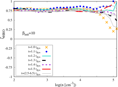
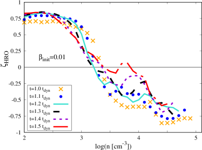
Figure 5: Relative orientation parameter, $\zeta_{\mathrm{HRO}}$, for simulation B10com (left) and B0.01com (right) as a function of density for various times between $t=t_{d}$ and $t=1.5\,t_{d}$. In case of run B10com, we also show very late stages up to $t=6.5\,t_{d}$ (thin grey lines). Apart from some expected temporal fluctuations, the relative orientation between the magnetic field and the density gradient reaches a quasi-stationary state.

4.6 Connection to observations

Lastly, we bridge the gap between our theoretical calculations and observations. For this task, we calculate the pseudo Stokes components (here given only for integration along the x-direction, Fiege & Pudritz, 2000)

$$q=\int{n\frac{B_{\mathrm{z}}^{2}-B_{\mathrm{y}}^{2}}{B^{2}}\mathrm{d}x},$$ (10)

$$u=2\int{n\frac{B_{\mathrm{z}}B_{\mathrm{y}}}{B^{2}}\mathrm{d}x}.$$ (11)

From these we calculate the polarisation angle

$$\chi=\frac{1}{2}\mathrm{arctan}\left(\frac{u}{q}\right)$$ (12)

and finally generate a pseudo polarisation vector $\underline{p}=p_{0}\left(\mathrm{sin}\chi\,\hat{\underline{e}}_{x}+\mathrm{cos}\chi\,\hat{\underline{e}}_{y}\right)$, where the $\hat{\underline{e}}_{i}$ vectors are the unit vectors along the directions perpendicular to the line of sight and $p_{0}=0.1$ is the maximum polarisation fraction.
The resulting HRO shape parameter as a function of gas column density is shown in Fig. 6. Comparison of these data with the shape parameter as a function of volume density in Fig. 2 reveals the large impact of projection effects along the line of sight for the scenarios with low initial magnetisation. Here, the orientation is seen to be parallel for the entire column density range. We remind the reader that in 3D it is actually vice versa, i.e. entirely perpendicular alignment between the magnetic field and the density gradients. We further find only minor differences between the runs with an initial magnetisation of $\beta=10$ and $\beta=1$ or between the lines of sight. A major difference appears when the gas is magnetically dominated. Here, the data reveal no preferred orientation at the lower column densities and an increasing alignment of the two fields at higher column densities. Interestingly, this decreasing trend is not observed as clearly in the solenoidal counterpart. However, here a clear difference is evident for the two different lines of sight. Whereas the integration perpendicular to the initial field reveals no preferred or at most a slight perpendicular alignment, the corresponding projection along the initial background field shows a pronounced parallel alignment. In addition, similar to the compressive case, no difference is seen for the low magnetisation cases.
The negative relative orientation parameter has also been found recently in synthetic observations by Seifried et al. (2020) for weakly magnetised media. We show in the bottom panel of Fig. 6 the retrieved shape parameter for the times already provided in Fig. 5. Whereas there appeared almost no fluctuations across a large density range in the volume density calculation, the corresponding projections strongly fluctuate both as a function of column density and time. In fact, the most striking feature is the absence of a preferred perpendicular alignment in projection. Instead, $\zeta_{\mathrm{HRO}}\sim 0$ seems to be the largest typical value in projection. This indicates that there appears no preferred orientation. Interestingly, the red line is observed to be quite similar to the case of a compressive turbulent velocity field and a strong magnetic field, again emphasising the role of projection effects. It is hence hard, if not impossible, to differentiate between compressive or solenoidal turbulence driving via the relative orientation of the magnetic field and (column-) density gradient.

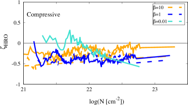
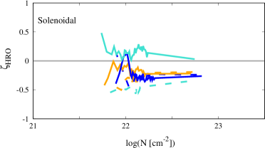
Figure 6: Shape parameter as a function of logarithmic column density for projections along the initial background magnetic field direction (dashed) and perpendicular to it (solid) for both compressive (top) and solenoidal (middle) turbulence driving. Colour denotes different initial magnetisation of the gas. Note that there are no data shown for integration along the x-direction for run B0.01com due to the too small column density range. The bottom panel shows the time evolution of the shape parameter for run B10com. Although the shape parameter never attains positive values over the entire column density range, it is evident that it fluctuates between almost no preferred and a slightly parallel orientation.

5 Summary and conclusions

We presented a study on the relative orientation between the magnetic field and the gas density gradient in non-gravitating, turbulent media with varying initial magnetisation. We considered numerical simulations where the turbulence is driven by an external forcing term either in a fully compressive or entirely solenoidal way. Our case study thus covers two extreme conditions of supersonic interstellar turbulence.

Our most important finding is that compressive o solenoidal turbulence alone does not induce a change in relative orientation between the magnetic field and the gas density gradient. The change in relative orientation reported in previous numerical studies that include self-gravity is only found in the simulations with the highest magnetization in our data set. The nature of the turbulent forcing of the velocity field only mildly affects the transition in the relative orientation. This suggests that, in agreement with previous numerical studies, the change in relative orientation primarily depends on the magnetisation of the gas.

The configuration where the magnetic field parallel to the gas density gradient, or parallel to the isodensity contours, is only observed clearly in the simulation with high magnetization and compressive turbulence. This is in agreement with the interpretation presented in Soler & Hennebelle (2017b), where the main driver of a change in relative orientation between the magnetic field and the density structures is the compression of the gas.

We studied the time evolution of the simulations and found that the relative orientation between the magnetic field and the gas density gradient does not significantly change within one dynamical time. In this quasi-steady state, the relative orientation depends only on the initial magnetisation of the gas. We conclude that a true change in relative orientation can only be achieved in a medium with a dynamically significant magnetic field.

Data availability

The data underlying this article will be shared on reasonable request to the corresponding authors.

Appendix A Time evolution of coefficients

As a support to our analysis, we provide in Figs. 7 and 8 the time evolution of the governing coefficients in eq. 1. These data show that the solutions are time independent and that such weakly magnetised systems will never manage to change its relative orientation.

Figure 7: Same as Fig. 3, but for the time evolution of only run B10com. Once, the system has reached a quasi-steady state, the parameters, which govern the rate of change of the angle between the magnetic and density gradient fields, do not vary much.

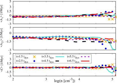
Figure 8: Density dependence of the individual parameters, which determine the rate of change of the relative orientation for run B10com. Different lines indicate different times. Once a quasi-stationary state is reached, the relative orientation does not change anymore.

References

- Beattie & Federrath (2020) Beattie J. R., Federrath C., 2020, MNRAS, 492, 668
- Beck (2015) Beck R., 2015, in Lazarian A., de Gouveia Dal Pino E. M., Melioli C., eds, Astrophysics and Space Science Library Vol. 407 of Astrophysics and Space Science Library, Magnetic Fields in Galaxies. p. 507
- Bouchut et al. (2009) Bouchut F., Klingenberg C., Waagan K., 2009, Numerische Mathematik
- Chen et al. (2016) Chen C.-Y., King P. K., Li Z.-Y., 2016, ApJ, 829, 84
- Chen et al. (2017) Chen C.-Y., Li Z.-Y., King P. K., Fissel L. M., 2017, ApJ, 847, 140
- Crutcher (2012) Crutcher R. M., 2012, ARA&A, 50, 29
- Dubey et al. (2008) Dubey A., Fisher R., Graziani C., Jordan IV G. C., Lamb D. Q., Reid L. B., Rich P., Sheeler D., Townsley D., Weide K., 2008, in Pogorelov N. V., Audit E., Zank G. P., eds, Numerical Modeling of Space Plasma Flows Vol. 385 of Astronomical Society of the Pacific Conference Series, Challenges of Extreme Computing using the FLASH code. pp 145–+
- Federrath et al. (2008) Federrath C., Klessen R. S., Schmidt W., 2008, ApJ, 688, L79
- Federrath et al. (2009) Federrath C., Klessen R. S., Schmidt W., 2009, ApJ, 692, 364
- Federrath et al. (2010) Federrath C., Roman-Duval J., Klessen R. S., Schmidt W., Mac Low M.-M., 2010, A&A, 512, A81
- Ferrière (2001) Ferrière K. M., 2001, Reviews of Modern Physics, 73, 1031
- Fiege & Pudritz (2000) Fiege J. D., Pudritz R. E., 2000, MNRAS, 311, 105
- Field (1965) Field G. B., 1965, ApJ, 142, 531
- Fissel et al. (2019) Fissel L. M., Ade P. A. R., Angilè F. E., Ashton P., Benton S. J., Chen C.-Y., Cunningham M., Devlin M. J., Dober B., Friesen R., Fukui Y., Galitzki 2019, ApJ, 878, 110
- Goldreich & Sridhar (1995) Goldreich P., Sridhar S., 1995, ApJ, 438, 763
- Hartmann et al. (2001) Hartmann L., Ballesteros-Paredes J., Bergin E. A., 2001, ApJ, 562, 852
- Heiles & Crutcher (2005) Heiles C., Crutcher R., 2005, in Wielebinski R., Beck R., eds, Cosmic Magnetic Fields Vol. 664 of Lecture Notes in Physics, Berlin Springer Verlag, Magnetic Fields in Diffuse HI and Molecular Clouds. p. 137
- Hennebelle & Inutsuka (2019) Hennebelle P., Inutsuka S.-i., 2019, Frontiers in Astronomy and Space Sciences, 6, 5
- Hennebelle & Pérault (2000) Hennebelle P., Pérault M., 2000, A&A, 359, 1124
- Hu et al. (2019) Hu Y., Yuen K. H., Lazarian A., 2019, ApJ, 886, 17
- Jow et al. (2018) Jow D. L., Hill R., Scott D., Soler J. D., Martin P. G., Devlin M. J., Fissel L. M., Poidevin F., 2018, MNRAS, 474, 1018
- Klessen & Glover (2016) Klessen R. S., Glover S. C. O., 2016, Star Formation in Galaxy Evolution: Connecting Numerical Models to Reality, Saas-Fee Advanced Course, Volume 43. ISBN 978-3-662-47889-9. Springer-Verlag Berlin Heidelberg, 2016, p. 85, 43, 85
- Koch et al. (2012) Koch P. M., Tang Y.-W., Ho P. T. P., 2012, ApJ, 747, 80
- Konstandin et al. (2012) Konstandin L., Girichidis P., Federrath C., Klessen R. S., 2012, ApJ, 761, 149
- Körtgen & Banerjee (2015) Körtgen B., Banerjee R., 2015, MNRAS, 451, 3340
- Körtgen et al. (2018) Körtgen B., Banerjee R., Pudritz R. E., Schmidt W., 2018, MNRAS, 479, L40
- Pattle & Fissel (2019) Pattle K., Fissel L., 2019, Frontiers in Astronomy and Space Sciences, 6, 15
- Planck Collaboration XXXV (2016) Planck Collaboration XXXV 2016, A&A, 586, A138
- Seifried et al. (2020) Seifried D., Walch S., Weis M., Reissl S., Soler J. D., Klessen R. S., Joshi P. R., 2020, MNRAS
- Soler (2019) Soler J. D., 2019, A&A, 629, A96