Perturbative approach for strong and weakly coupled time-dependent non-Hermitian quantum systems

Abstract:

We propose a perturbative approach to determine the time-dependent Dyson map and the metric operator associated with time-dependent non-Hermitian Hamiltonians. We apply the method to a pair of explicitly time-dependent two dimensional harmonic oscillators that are weakly coupled to each other in a PT-symmetric fashion and to the strongly coupled explicitly time-dependent negative quartic anharmonic oscillator potential. We demonstrate that once the perturbative Ansatz is set up the coupled differential equations resulting order by order may be solved recursively in a constructive manner, thus bypassing the need for making any guess for the Dyson map or the metric operator. Exploring the ambiguities in the solutions of the order by order differential equations naturally leads to a whole set of inequivalent solutions for the Dyson maps and metric operators implying different physical behaviour as demonstrated for the expectation values of the time-dependent energy operator.

1 Introduction

The key ingredient for a physical interpretation of $\mathcal{PT}$-symmetric/pseudo Hermitian Hamiltonian systems requires a well defined positive definite metric operator $\rho$. Only when this operator is explicitly known one is in a position to define a positive definite inner product, calculate observables together with their expectation values and thus root the non-Hermitian theory in a well defined Hilbert space [1, 2, 3, 4]. In the absence of an explicit time-dependence in the non-Hermitian Hamiltonian $H\neq H^{\dagger}$ the metric operator $\rho$ can be determined from the time-independent quasi-Hermiticity relation $H^{\dagger}\rho=\rho H$; in principle that is. The metric operator can be factorised as $\rho=\eta^{\dagger}\eta$, where $\eta$ is often referred to as the Dyson map. The adjoint action of this operator maps the non-Hermitian Hamiltonian to a Hermitian counterpart $h=h^{\dagger}$ by mean of the time-independent Dyson equation $\eta H\eta^{-1}=h$.

For many known models the metric, and therefore the Dyson map, have been constructed in an explicitly analytically closed form, see for instance [5, 6, 7, 8, 9]. However, in general these “solvable models” remain an exception and one often needs to employ a perturbative approach in order to gain some insight into the theory. Even for the classic example of a non-Hermitian system with a real eigenvalue spectrum, complex cubic oscillator potential $V=ix^{3}$, the metric operator is only known in a perturbative form [10, 11]. This approach has turned out to be very successful and there are even examples for which an initially perturbative approach has led to an exact solution with the perturbation series terminating at a certain order, see e.g. [5] for the unstable quartic anharmonic oscillator potential $V=-x^{4}$.

When an explicit time-dependence is introduced into the Hamiltonians $h(t)=h(t)^{\dagger}$ and $H(t)\neq H(t)^{\dagger}$, one needs to solve the two time-dependent Schrödinger equations $i\hbar\partial_{t}\phi(t)=h(t)\phi(t)$ and $i\hbar\partial_{t}\psi(t)=H(t)\psi(t)$. Assuming that the two associated wave functions are related as $\phi(t)=\eta(t)\psi(t)$, one easily derives [12, 13, 14, 15, 16, 17, 18] that the corresponding time-dependent Dyson equation (TDDE) and time-dependent quasi-Hermiticity relation (TDQH) acquire the forms

$$h(t)=\eta(t)H(t)\eta^{-1}(t)+i\hbar\partial_{t}\eta(t)\eta^{-1}(t)\text{, \ \ \ }H^{\dagger}(t)=\rho(t)H(t)\rho^{-1}(t)+i\hbar\partial_{t}\rho(t)\rho^{-1}(t),$$ (1)

respectively. The novelty in the conceptual interpretation of these equations is the fact that the non-Hermitian Hamiltonian $H(t)$, defined as the operator that satisfies the time-dependent Schrödinger equations, ceases to be an observable corresponding to the energy as it is no longer pseudo Hermitian, i.e. related to a Hermitian operator by means of a similarity transformation. Instead, the time-dependent observable energy operator was identified as

$$\tilde{H}(t):=\eta^{-1}(t)h(t)\eta(t)=H(t)+i\hbar\eta^{-1}(t)\partial_{t}\eta(t).$$ (2)

Evidently, to solve the two equations (1) for $\eta(t)$ and $\rho(t)$ is more complicated than solving those for the time-independent case, due to the presence of the additional time derivative terms. Nonetheless, for several concrete examples exact solutions to these equations have been constructed [17, 19, 20, 21, 22, 23, 24]. An alternative new approach, that utilizes the Lewis Riesenfeld method of invariants [25], has recently been developed [26, 27]. The advantage of this approach is that once the invariants are constructed it becomes much simpler to solve for the time-dependent Dyson map as there is no additional time derivative term in the relevant equations. All these approaches rely on certain inspired guesses for a suitable Ansatz of the metric or the Dyson map. In contrast, the powerful feature of the time-independent perturbative approach mentioned above is that it is entirely constructive and may be solved order by order. So far no such perturbative approach has been developed or applied in the time-dependent scenario. The main purpose of this paper is to develop such an approach and explore its viability to find solutions to the equations (1) for $\eta(t)$ and $\rho(t)$. In particular, we seek to answer the question of whether it is possible to apply such an approach recursively order by order in a constructive fashion.

Besides the proposed technical advance we expect any new solution to reveal or confirm some newly observed physical phenomena. In [28] the remarkable and unexpected feature was found that the region in parameter space, usually referred to as the spontaneously $\mathcal{PT}$-broken regime, becomes physical when transgressing from the time-independent to the time-dependent scenario. This regime is characterised by a $\mathcal{PT}$-symmetric Hamitonian for which the corresponding wavefunctions are $\mathcal{PT}$-symmetrically broken. As a consequence the energy eigenvalues occur in complex conjugate pairs in the time-independent case. However, in the time-dependent case the expectation values for the energy operator $\tilde{H}(t)$ have been found to be real for some models in that regime and the two regimes are distinguished by qualitatively quite different types of behaviour. Besides the energy also other physical quantities display unusual physical behaviour, such as for instance the entropy [29, 30, 31]. So far all explicit solutions constructed thereafter have confirmed these charcteristics, but up to now a generic argument that explains the occurrence of them is still missing. We expect that even solutions to the metric operator that are only known perturbatively to some finite order will provide insight into these features.

Our manuscript is organized as follows: In order to set the scene and to establish our notations we briefly recall in section 2 the perturbative approach to determine the metric operator for time-independent non-Hermitian Hamiltonian quantum systems. We then present our proposal for a perturbation theory for the explicitly time-dependent scenario. In section 3 we apply the proposed method to a pair of explicitly time-dependent two dimensional harmonic oscillators that are weakly coupled to each other in a PT-symmetric fashion and in section 4 to the strongly coupled negative quartic anharmonic oscillator potential with an explicit time-dependence. In section 5 we present our conclusions and outlook.

2 Perturbative expansions for the metric and the Dyson map

2.1 Time-independent perturbation theory

We start by recalling the time-independent perturbation theory for determining the time-independent metric and Dyson map [32, 33, 5, 12]. We start by separating the non-Hermitian Hamiltonian into its real and imaginary part as

$$H=h_{0}+i\epsilon h_{1},\qquad\ \ \text{with}~{}h_{0}^{\dagger}=h_{0},h_{1}^{\dagger}=h_{1},$$ (3)

where a real parameter $\epsilon\ll 1$ has been extracted from the imaginary part. Assuming here for simplicity that the Dyson map is Hermitian and of the form $\eta=e^{q/2}$, the metric operator just becomes $\rho=\eta^{\dagger}\eta=\eta^{2}=e^{q}$. Making use of the standard Baker-Campbell-Hausdorff formula

$$e^{A}Be^{-A}=B+[A,B]+\frac{1}{2!}[A,[A,B]]+\frac{1}{3!}[A,[A,[A,B]]]+...$$ (4)

and assuming that $\rho$ is invertible one can then write the quasi-Hermiticity relation as

$$H^{\dagger}=\eta^{2}H\eta^{-2}=H+[q,H]+\frac{1}{2!}[q,[q,H]]+\frac{1}{3!}[q,[q,[q,H]]]+...$$ (5)

Using the decomposition (3) for the non-Hermitian Hamiltonian $H$ this becomes

$$i[q,h_{0}]+\frac{i}{2}[q,[q,h_{0}]]+\frac{i}{3!}[q,[q,[q,h_{0}]]]+...=\epsilon\left(2h_{1}+[q,h_{1}]+\frac{1}{2}[q,[q,h_{1}]]+...\right).$$ (6)

Expanding $q$ further as a power series in $\epsilon$ in the form

$$q=\sum_{n=1}^{\infty}\epsilon^{n}q_{n},$$ (7)

one can read off the coefficients of $\epsilon^{n}$ order by order upon substituting (7) into (6). One finds that $[h_{0},q_{2}]=0$, so that with the choice $q_{2}=0$ all even powers in (7) vanish. The first three nonvanishing equations are

$$[h_{0},q_{1}] =2ih_{1},$$ (8)

$$[h_{0},q_{3}] =\frac{i}{6}[q_{1},[q_{1},h_{1}]],$$ (9)

$$[h_{0},q_{5}] =\frac{i}{6}\left([q_{1},[q_{3},h_{1}]]+[q_{3},[q_{1},h_{1}]]-\frac{1}{60}[q_{1},[q_{1},[q_{1},[q_{1},h_{1}]]]]\right).$$ (10)

Crucially, these equations provide a constructive scheme and can be solved recursively order by order for $q_{1}$, $q_{2}$, … At each order one may add a term to $q_{i}$ that commutes with $h_{0},$ which, however, does not change the resulting Hermitian Hamiltonian $h$. One may even find a closed formula for the expression of $h$ involving Euler’s number [12]. The metric operator is well-known not to be unique. This feature is inherited in the time-dependent setting as will be demonstrated below.

2.2 Time-dependent perturbation theory

We shall now propose a similar procedure as in the time-independent case, however, we solve the time-dependent quasi-Hermiticity relation in (1) for $\rho(t)$ rather than the time-dependent Dyson equation for $\eta(t)$. We separate the Hamiltonian as

$$H(t)=h_{0}(t)+i\epsilon h_{1}(t),\qquad\ \ \text{with}~{}h_{0}(t)=h_{0}^{\dagger}(t),h_{1}(t)=h_{1}^{\dagger}(t),$$ (11)

with $\epsilon\ll 1$ being a time-independent expansion parameter. The time-dependent Dyson map is assumed to be of the form

$$\eta(t)=e^{q(t)/2}=\prod_{i=1}^{j}\exp\left(\sum_{l=1}^{\infty}\epsilon^{l}\gamma_{i}^{(l)}(t)q_{i}^{(l)}\right).$$ (12)

At this point $\gamma_{i}^{(l)}(t)$ are time-dependent real functions, $q_{i}^{(l)}$ are operators and the limit $j\in\mathbb{N}$ is subject to a suitable choice. The product in (12) is understood to be ordered $\prod_{i=1}^{j}a_{i}=a_{1}a_{2}\ldots a_{j}$. For the special choice $q_{i}^{(1)}=q_{i}^{(2)}=...=q_{i}^{(l)}=q_{i}=q_{i}^{\dagger}$, the exponential of the sum becomes a product of exponentials and the metric acquires the form

$$\rho(t)=\eta(t)^{\dagger}\eta(t)=\prod_{i=j}^{1}\left[\prod_{l=k}^{1}\exp\left(\epsilon^{l}\gamma_{i}^{(l)}q_{i}\right)\right]\prod_{i=1}^{j}\left[\prod_{l=1}^{k}\exp\left(\epsilon^{l}\gamma_{i}^{(l)}q_{i}\right)\right],$$ (13)

where $\prod_{i=j}^{1}$ denotes the reverse ordered product, that is $\prod_{i=j}^{1}a_{i}=a_{j}a_{j-1}\ldots a_{1}$. We have also terminated the infinite sum in (12) at a finite value $k$. For $k=1$ the relevant terms in the metric are therefore identified to be

$$\rho^{(1)}(t)=\left[\prod_{i=j}^{1}\exp\left(\epsilon\gamma_{i}^{(1)}q_{i}\right)\right]\left[\prod_{i=1}^{j}\exp\left(\epsilon\gamma_{i}^{(1)}q_{i}\right)\right].$$ (14)

Upon substituting this expression into the time-dependent quasi-Hermiticity relation in (1), and expanding up to first order in $\epsilon$ we obtain the first order differential equation

$$ih_{1}+\sum_{i=1}^{j}\left(\gamma_{i}^{(1)}\left[q_{i},h_{0}\right]+i\dot{\gamma}_{i}^{(1)}q_{i}\right)=0.$$ (15)

We observe from this equation that we can multiply the Dyson map by a factor involving a time-independent phase that commutes with the Hermitian part of the Hamiltonian. This is analogous to time-independent first order equation (8), which can be retrieved from (15) by setting the time-derivative terms to zero with $j=1$ and $\gamma_{1}^{(1)}=1/2$.

To second order the relevant metric results to

$$\rho^{(2)}(t)=\prod_{i=j}^{1}\left[\prod_{l=2}^{1}\exp(\epsilon^{l}\gamma_{i}^{(l)}q_{i})\right]\prod_{i=1}^{j}\left[\prod_{l=1}^{2}\exp(\epsilon^{l}\gamma_{i}^{(l)}q_{i})\right],$$ (16)

where this time we have only kept terms up to order $\epsilon^{2}$ in the argument of the exponential function. We substitute this into the time-dependent quasi-Hermiticity relation in (1), and only keep terms that are proportional to $\epsilon^{2}$, obtaining

$$2\sum_{i=1}^{j}\left(\gamma_{i}^{(2)}[q_{i},h_{0}]+i\gamma_{i}^{(1)}[q_{i}^{1},h_{1}]+\frac{1}{2!}(\gamma_{i}^{(1)})^{2}[q_{i},[q_{i},h_{0}]]+i\dot{\gamma}_{i}^{(2)}q_{i}\right)$$

$$+\sum_{i=1}^{j}\left(2\sum_{r=1,\neq i}^{j}\left(\gamma_{i}^{(1)}\gamma_{r}^{(1)}[q_{r},[q_{i},h_{0}]]+i\dot{\gamma}_{i}^{(1)}\gamma_{r}^{(1)}[q_{r},q_{i}]\right)+(\gamma_{i}^{(1)})^{2}[q_{i},[q_{i},h_{0}]]\right)=0.$$ (17)

The equations resulting from higher order in $\epsilon$ can be derived in a similar fashion. Similar to the time-independent case, these equations can be solved recursively order by order. In contrast, we find here that the even ordered equations are also important, as will be demonstrated below.

Some remarks are in order with regards to the Ansatz made for the perturbative series. First of all we assumed here that $\eta(t)$ is Hermitian, which is not necessary and in fact implies that we are missing some of the solutions as we shall see below. The second point to notice is that we have not made any assumptions about the operators in the exponentials, which are in turn determined by (15), (16) and the corresponding higher order equations. Nonetheless, we made some assumptions about the form of the products. The factorized form is motivated by the fact that we need to compute time derivatives of these expansions, which makes expressions of the form $e^{A(t)+B(t)}$ with non vanishing commutators $[A(t),B(t)]$ unsuitable. We also need to make an assumption about the limits in the product. Let us now demonstrate for a concrete example that the recursive solutions of the order by order equations (15), (16), … do indeed lead to meaningful solutions of the time-dependent quasi-Hermiticity relation in (1).

3 Time-dependent coupled non-Hermitian harmonic oscillators

As a starting point to demonstrate the effectiveness of this perturbative approach we shall consider the following pair of time-dependent harmonic oscillators with a Hermitian and a non-Hermitian coupling term

$$H(t)=\frac{a(t)}{2}(p_{x}^{2}+x^{2})+\frac{b(t)}{2}(p_{y}^{2}+y^{2})+i\frac{\lambda(t)}{2}(xy+p_{x}p_{y})+\frac{\mu(t)}{2}(xp_{y}-yp_{x}),$$ (18)

involving the time-dependent coefficient functions $a(t)$, $b(t)$, $\lambda(t)$, $\mu(t)\in\mathbb{R}$. This non-Hermitian Hamiltonian is symmetric with respect to two different $\mathcal{PT}$-transformations, $[\mathcal{PT}_{\pm},H]=0$, where the antilinear maps are given by, $\mathcal{PT}_{\pm}:x\rightarrow\pm x,y\rightarrow\mp y,p_{x}\rightarrow\mp p_{x},p_{y}\rightarrow\pm p_{y},i\rightarrow-i$. It generalizes a system previously studied in [26] for $\mu=0$, $a=b$ and can be re-expressed in terms of Hermitian generators, $K_{i}^{\dagger}=K_{i}$,

$$K_{1}=\frac{1}{2}(p_{x}^{2}+x^{2}),\quad K_{2}=\frac{1}{2}(p_{y}^{2}+y^{2}),\quad K_{3}=\frac{1}{2}(xy+p_{x}p_{y}),\quad K_{4}=\frac{1}{2}(xp_{y}-yp_{x}),$$ (19)

forming a closed algebra with commutation relations

$$\left[K_{1},K_{2}\right]=0, \left[K_{1},K_{3}\right]=iK_{4},\qquad \left[K_{1},K_{4}\right]=-iK_{3},$$

$$\left[K_{2},K_{3}\right]=-iK_{4},~{}~{}~{} \left[K_{2},K_{4}\right]=iK_{3},\qquad \left[K_{3},K_{4}\right]=i(K_{1}-K_{2})/2.$$ (20)

Thus we may rewrite the Hamiltonian $H(t)$ in terms of these generators simply as

$$H(t)=a(t)K_{1}+b(t)K_{2}+i\lambda(t)K_{3}+\mu(t)K_{4}.$$ (21)

Denoting $c(t):=a(t)-b(t)$, we shall be considering the three different cases for $H(t)$, characterized as:

$$\text{case 1}:\quad c(t)=0\quad\text{and}\quad\mu(t)=0,$$ (22)

$$\text{case 2}:\quad c(t)\neq 0\quad\text{and}\quad\mu(t)=0,$$ (23)

$$\text{case 3}:\quad c(t)=0\quad\text{and}\quad\mu(t)\neq 0.$$ (24)

The first order perturbation equation (15) that needs to be satisfied has many different types of solutions for each of these cases. Therefore we shall present the different solutions in separate sections below. We will also discuss the possibility of $\eta^{\dagger}\neq\eta$ captured by letting some of the coefficient functions $\gamma_{i}^{(l)}$ to be purely imaginary.

As noticed in [20, 26], an interesting feature of the explicitly time-dependent systems is that the spontaneously broken regime of the time-independent system becomes physical. To see whether this is also the case here we briefly discuss the time-independent version of the Hamiltonian (21) with $\dot{a}=\dot{b}=\dot{\lambda}=\dot{\mu}=0$ in order to create a benchmark for the $\mathcal{PT}$-broken and $\mathcal{PT}$-symmetric regions in the parameter space. Taking the Dyson map to be of the form

$$\eta=\exp(\theta K_{4}),\qquad\text{with \ \ }\theta=\mathop{\mathrm{a}rctanh}\left(-\frac{\lambda}{c}\right),$$ (25)

and acting adjointly on $H$ leads to the Hermitian Hamiltonian

$$h=\eta H\eta^{-1}=\frac{1}{2}\left(a+b\right)(K_{1}+K_{2})+\frac{1}{2}\sqrt{c^{2}-\lambda^{2}}(K_{1}-K_{2})+\mu K_{4},$$ (26)

with eigenvalues

$$E_{n,m}=\frac{1}{2}(1+n+m)(a+b)+\frac{1}{2}(n-m)\sqrt{c^{2}-\lambda^{2}}\sqrt{1+\frac{\mu^{2}}{c^{2}-\lambda^{2}}}.$$ (27)

We notice for the cases 1 and 3, that is when $c=0$, the Dyson map is ill-defined and also the eigenvalues are complex so that these two cases are always in the spontaneously broken $\mathcal{PT}$-regime. For case 2 we identify a $\mathcal{PT}$-symmetric regime when $|\lambda|<|c|$ and a spontaneously broken regime otherwise. Let us now demonstrate that the spontaneously broken $\mathcal{PT}$-regimes can become physical when an explicit time-dependence is introduced.

We need to treat the cases 1 and 2 separately from the case 3, as we find that the perturbative expansions for the metric have no common overlap.

3.1 Metric and Dyson maps with $\mu(t)=0$, cases 1 and 2

We will now show how the above perturbative equations can be solved systematically order by order in $\epsilon$. We treat here the non-Hermitian term as a small perturbation and set $\lambda(t)\rightarrow\epsilon\lambda(t)$ with $\epsilon\ll 1$. When succeeding in constructing a complete infinite series we may set $\epsilon$ back to $1$. Focusing at first on the cases 1 and 2 with $\mu(t)=0$, the first order equation (15) for the Hamiltonian $H(t)$ in (21) becomes

$$i\lambda(t)K_{3}+\sum_{i=1}^{j}\left(\gamma_{i}^{(1)}\left[q_{i},a(t)K_{1}+b(t)K_{2}\right]+i\dot{\gamma}_{i}^{(1)}q_{i}\right)=0.$$ (28)

When compared to the corresponding time-independent equation (8), we notice that besides having to satisfy the commutative structure, the coefficient functions are not just a set of functions of the parameters in the model, but correspond now to a system of coupled differential equations. Having the options in (28) to take $j\in\{1,2,3,4\}$ with $q_{i}\in\{K_{1},K_{2},K_{3},K_{4}\}$, the first order equation becomes

$$i\left(\lambda+c\gamma_{1}^{(1)}+\dot{\gamma}_{2}^{(1)}\right)K_{3}+i\left(\dot{\gamma}_{1}^{(1)}-c\gamma_{2}^{(1)}\right)K_{4}+i\dot{\gamma}_{3}^{(1)}K_{1}+i\dot{\gamma}_{4}^{(1)}K_{2}=0.$$ (29)

Thus setting the coefficients of all $K_{i}$ in (29) to zero, we obtain two coupled first order equations for $\gamma_{1}^{(1)}$ and $\gamma_{2}^{(1)}$. Moreover, we conclude that $\gamma_{3}^{(1)}$ and $\gamma_{4}^{(1)}$ are time-independent. As our goal is to find a time-dependent metric and Dyson map we set them both to zero $\gamma_{3}^{(1)}=\gamma_{4}^{(1)}=0$. Having now fixed $j=2$ and the corresponding $q_{1}=K_{4}$, $q_{2}=K_{3}$, we can simply evaluate the higher order equations obtaining the constraints by setting the coefficient functions to zero. The first equation contains the key foundational structure for the entire series.

We proceed now in this manner to the higher order equations.

3.1.1 Hermitian $\eta$ with $q_{1}=K_{4}$ and $q_{2}=K_{3}$

Keeping now the choice of the $q_{i}$ as indicated above, we derive the differential equations to be satisfied at each order in $\epsilon$. The first five orders of the equations to be satisfied for the $\gamma_{1}^{(l)}(t)$ are

$$\epsilon^{1}:\quad\dot{\gamma}_{1}^{(1)}=c\gamma_{2}^{(1)},$$ (30)

$$\epsilon^{2}:\quad\dot{\gamma}_{1}^{(2)}=c\gamma_{2}^{(2)},$$ (31)

$$\epsilon^{3}:\quad\dot{\gamma}_{1}^{(3)}=c\left[\frac{1}{6}\left(\gamma_{2}^{(1)}\right)^{3}+\gamma_{2}^{(3)}\right],$$ (32)

$$\epsilon^{4}:\quad\dot{\gamma}_{1}^{(4)}=c\left[\frac{1}{2}\left(\gamma_{2}^{(1)}\right)^{2}\gamma_{2}^{(2)}+\gamma_{2}^{(4)}\right],$$ (33)

$$\epsilon^{5}:\quad\dot{\gamma}_{1}^{(5)}=c\left[\frac{1}{120}\left(\gamma_{2}^{(1)}\right)^{5}+\frac{1}{2}\gamma_{2}^{(1)}\left(\gamma_{2}^{(2)}\right)^{2}+\frac{1}{2}\left(\gamma_{2}^{(1)}\right)^{2}\gamma_{2}^{(3)}+\gamma_{2}^{(5)}\right].$$ (34)

For $\gamma_{2}(t)$ we obtain the first order differential equations

$$\epsilon^{1}:\quad\dot{\gamma}_{2}^{(1)}=-c\gamma_{1}^{(1)}-\lambda,$$ (35)

$$\epsilon^{2}:\quad\dot{\gamma}_{2}^{(2)}=-c\gamma_{1}^{(2)},$$ (36)

$$\epsilon^{3}:\quad\dot{\gamma}_{2}^{(3)}=c\left[\frac{1}{3}\left(\gamma_{1}^{(1)}\right)^{3}-\gamma_{1}^{(3)}-\frac{1}{2}\gamma_{1}^{(1)}\left(\gamma_{2}^{(1)}\right)^{2}\right],$$ (37)

$$\epsilon^{4}:\quad\dot{\gamma}_{2}^{(4)}=c\left[\left(\gamma_{1}^{(1)}\right)^{2}\gamma_{1}^{(2)}-\gamma_{1}^{(4)}-\frac{1}{2}\gamma_{1}^{(2)}\left(\gamma_{2}^{(1)}\right)^{2}-\gamma_{1}^{(1)}\gamma_{2}^{(1)}\gamma_{2}^{(2)}\right],$$ (38)

$$\epsilon^{5}:\quad\dot{\gamma}_{2}^{(5)}=c\left[\gamma_{1}^{(1)}\left(\gamma_{1}^{(2)}\right)^{2}-\frac{2}{15}\left(\gamma_{1}^{(1)}\right)^{5}+\left(\gamma_{1}^{(1)}\right)^{2}\gamma_{1}^{(3)}-\gamma_{1}^{(5)}+\frac{1}{6}\left(\gamma_{1}^{(1)}\right)^{3}\left(\gamma_{2}^{(1)}\right)^{2}\right.$$ (39)

$$\qquad\qquad\quad\!\!\left.-\frac{1}{24}\gamma_{1}^{(1)}\left(\gamma_{2}^{(1)}\right)^{4}-\frac{1}{2}\gamma_{1}^{(3)}\left(\gamma_{2}^{(1)}\right)^{2}-\gamma_{1}^{(2)}\gamma_{2}^{(1)}\gamma_{2}^{(2)}-\frac{1}{2}\gamma_{1}^{(1)}\left(\gamma_{2}^{(2)}\right)^{2}-\gamma_{1}^{(1)}\gamma_{2}^{(1)}\gamma_{2}^{(3)}\right].$$

These equations reveal the underlying structure that distinguishes the different cases. Whilst the equations look rather complex, they contain all the information that can be used to obtain the solutions up to fifth order that can even be extrapolated to the exact solutions.

From perturbation theory to the exact Dyson map and Hermitian Hamiltonians

We shall now demonstrate how to use these equations to obtain the Dyson map and hence the metric. Proceeding similarly as for the first order equation (29), we may solve the set of equations (30)-(34), (35)-(39) recursively order by order to obtain the explicit expressions for the coefficient functions $\gamma_{1}^{(i)}(t)$ and $\gamma_{2}^{(i)}(t)$, $i=1,2,\ldots$ We will not report these expressions here. In the next step we extrapolate from the first terms by trying to identify a combination of standard functions whose Taylor expansion matches the first terms in the perturbative series.

For case 1, when $c(t)=0$, we notice from (29) that also $\dot{\gamma}_{1}^{(1)}=0$ when requiring Hermiticity of $h$. As the Hermitian part of the Hamiltonian $H(t)$ is given by $h_{0}(t)=a(t)(K_{1}+K_{2})$, we now have $[h_{0}(t),K_{i}]$ so that all of the generators in this algebra commute with $h_{0}(t)$. As a consequence of this we observe that all orders of the perturbation equations disappear except for one. This is also seen by setting $c=0$ in (30)-(39) so that the only relevant equation left is

$$\dot{\gamma}_{2}^{(1)}(t)=-\lambda(t).$$ (40)

Hence, we easily obtain the exact solution

$$\gamma_{1}^{(1)}(t)=\gamma_{1}(t)=k_{1},\qquad\gamma_{2}^{(1)}(t)=\gamma_{2}(t)=-\int^{t}\lambda(s)ds+k_{2},$$

with two integration constants $k_{1}$, $k_{2}$.

For case 2, when $c(t)\neq 0$, all of the right hand sides of the differential equations are proportional to $c(t)$, except for the one for $\dot{\gamma}_{2}^{(1)}(t)$ in (35). Assuming $\lambda(t)$ to be a real multiple of $c(t)$ the equations become fully integrable and we are able to solve the equations order by order, even leading to an exact solution. Keeping for instance terms up to fifth order we obtain

$$\left[\dot{\gamma}_{1}(t)\right]^{\left[5\right]}=\sum_{i=1}^{5}\epsilon^{i}\dot{\gamma}_{1}^{(i)}(t)=c(t)\left[\epsilon\sinh\left(\sum_{i=1}^{5}\epsilon^{i}\gamma_{2}^{(i)}(t)\right)\right]^{\left[5\right]}=c(t)\left\{\epsilon\sinh\left[\gamma_{2}(t)\right]\right\}^{\left[5\right]},$$ (41)

and

$$\left[\dot{\gamma}_{2}(t)\right]^{\left[5\right]} =\sum_{i=1}^{5}\epsilon^{i}\dot{\gamma}_{2}^{(i)}(t)=-\lambda(t)-c(t)\left\{\epsilon\left[\cosh\left(\sum_{i=1}^{5}\epsilon^{i}\gamma_{2}^{(i)}(t)\right)\right]\left[\tanh\left(\sum_{i=1}^{5}\epsilon^{i}\gamma_{1}^{(i)}(t)\right)\right]\right\}^{\left[5\right]}$$

$$=-\lambda(t)-c(t)\left(\epsilon\cosh[\gamma_{2}(t)]\tanh[\gamma_{1}(t)]\right)^{\left[5\right]}.$$ (42)

Here the superscript $\left[5\right]$ means we only retain terms up to order 5 in $\epsilon$. In fact, we have verified the validity of the closed form to eleventh order, by extending and solving the sets of equations (30)-(34) and (35)-(39).

Assuming now the expressions in (41) and (42) to be exact, we may set $\epsilon=1$ and subsequently solve them for $\gamma_{1}(t)$ and $\gamma_{2}(t)$. Letting $\lambda(t)$ be any real multiple of $c(t)$, that is

$$c(t)=p\lambda(t)\qquad\text{where}\qquad p\in\mathbb{R},$$ (43)

we are able to solve the relevant equations exactly and express $\gamma_{2}$ as a function of $\gamma_{1}$ as

$$\gamma_{2}(\gamma_{1})=\pm\mathop{\mathrm{a}rccosh}\left\{-\frac{1}{2}\mathop{\mathrm{s}ech}(\gamma_{1})\left[k_{1}+\frac{2}{p}\sinh(\gamma_{1})\right]\right\},$$ (44)

with $k_{1}$ being an integration constant. Relation (44) is obtained by integrating $\dot{\gamma}_{2}/\dot{\gamma}_{1}=\partial\gamma_{2}/\partial\gamma_{1}$ with respect to $\gamma_{1}$. Parameterizing $\gamma_{1}(t)$ by a new function $\chi(t)$ as

$$\gamma_{1}=\mathop{\mathrm{a}rcsinh}\left(\chi\right),$$ (45)

the two differential equations for $\dot{\gamma}_{1}(t)$ and $\dot{\gamma}_{2}(t)$ can be converted into the linear second order equation entirely in $\chi$

$$\ddot{\chi}-\frac{\dot{\lambda}}{\lambda}~{}\dot{\chi}+(p^{2}-1)\lambda^{2}\chi=k_{1}\frac{p}{2}\lambda^{2}.$$ (46)

We solve equation (46) by

$$\chi(t)=\frac{e^{-2\sqrt{1-p^{2}}\left(k_{2}-\frac{1}{2}\int^{t}\lambda(s)ds\right)}}{4\left(1-p^{2}\right)}\left[\left(e^{2\sqrt{1-p^{2}}\left(k_{2}-\frac{1}{2}\int^{t}\lambda(s)ds\right)}-pk_{1}\right)^{2}+(k_{1}^{2}-4)\left(1-p^{2}\right)\right].~{}$$ (47)

Notice that in fact we are solving the two first order equations for $\dot{\gamma}_{1}(t)$ and $\dot{\gamma}_{2}(t)$, so that there are only two integration constants and no additional linear independent solution for the second order equation (46). We have to impose here $\left|p\right|<1$ to ensure the reality of $\chi$ and hence $\gamma_{2}$, $\gamma_{1}$.

Having obtained an exact Dyson map, we can envoke the first equation in (1) and compute the Hermitian counterparts to $H(t)$, which consists of two decoupled harmonic oscillators in both cases 1 and 2

$$h(t)=f_{+}(t)K_{1}+f_{-}(t)K_{2}.$$ (48)

For case 1 we find $f_{\pm}(t)=a$ and for case 2 we obtain

$$f_{\pm}(t)=b+\frac{p\lambda}{2}\mp\frac{\lambda(2\chi+pk_{1})}{4(1+\chi^{2})}.$$ (49)

We may also compute real time-dependent energy expectation values from these expressions as will be shown below.

3.1.2 Non-Hermitian $\eta$ with $q_{1}=K_{4}$ and $q_{2}=K_{1},K_{2}$

Making now the choice $q_{1}=K_{4}$, $q_{2}=K_{1},K_{2}\,$ the perturbative expansion yields $\dot{\gamma}_{1}^{(l)}=\dot{\gamma}_{2}^{(l)}=0$, so that the entire metric becomes time-independent. However, $\eta$ does not have to be Hermitian as assumed in the Ansatz (12). Thus allowing $\gamma_{i}^{(l)}\in\mathbb{C}$ in general, we now modify the Ansatz to $\gamma_{1}^{(\ell)}\in\mathbb{R}$,  $\ell=1,2,\ldots$, $\gamma_{2}^{(\ell)}\in i\mathbb{R}$,  $\ell=0,1,2,\ldots$, $\gamma_{3}^{(\ell)}=\gamma_{4}^{(\ell)}=0.$ The perturbative constraints up to order $\epsilon^{3}$ then read

$$\epsilon^{1}:\quad\dot{\gamma}_{1}^{(1)}=\lambda\sin\left(\gamma_{2}^{(0)}\right),$$ (50)

$$\epsilon^{2}:\quad\dot{\gamma}_{1}^{(2)}=\lambda\gamma_{2}^{(1)}\cos\left(\gamma_{2}^{(0)}\right),$$ (51)

$$\epsilon^{3}:\quad\dot{\gamma}_{1}^{(3)}=\lambda\gamma_{2}^{(2)}\cos\left(\gamma_{2}^{(0)}\right)-\frac{1}{2}\lambda\left(\gamma_{2}^{(1)}\right)^{2}\sin\left(\gamma_{2}^{(0)}\right),$$ (52)

and for $\gamma_{2}(t)$ we obtain

$$\epsilon^{1}:\quad\dot{\gamma}_{2}^{(0)}=c+\lambda\frac{\cos\left(\gamma_{2}^{(0)}\right)}{\gamma_{1}^{(1)}},$$ (53)

$$\epsilon^{2}:\quad\dot{\gamma}_{2}^{(1)}=-\frac{\lambda}{\gamma_{1}^{(1)}}\left[\frac{\gamma_{1}^{(2)}}{\gamma_{1}^{(1)}}\cos\left(\gamma_{2}^{(0)}\right)+\gamma_{2}^{(1)}\sin\left(\gamma_{2}^{(0)}\right)\right],$$ (54)

$$\epsilon^{3}:\quad\dot{\gamma}_{2}^{(2)}=\frac{\lambda}{\gamma_{1}^{(1)}}\left\{\left[\frac{\left(\gamma_{1}^{(1)}\right)^{2}}{3}+\left(\frac{\gamma_{1}^{(2)}}{\gamma_{1}^{(1)}}\right)^{2}-\frac{\gamma_{1}^{(3)}}{\gamma_{1}^{(1)}}-\frac{\gamma_{2}^{(1)}}{2}\right]\cos\left(\gamma_{2}^{(0)}\right)\right.$$ (55)

$$\qquad\qquad\qquad+\left.\left[\frac{\gamma_{1}^{(2)}\gamma_{2}^{(1)}}{\gamma_{1}^{(1)}}-\gamma_{2}^{(2)}\right]\sin\left(\gamma_{2}^{(0)}\right)\right\}.$$

From perturbation theory to the exact Dyson map and Hermitian Hamiltonians

Once again we may solve these equations order by order for the coefficient functions $\gamma_{i}^{(\ell)}$ and subsequently try to extrapolate the series to all orders. We find the exact constraining equations for $\gamma_{1}(t)$ and $\gamma_{2}(t)$ by demanding the non-Hermitian terms in $h(t)$ to vanish

$$\dot{\gamma}_{1}=\lambda\sin\left(\gamma_{2}\right),\quad~{}~{}\text{and\quad~{}}\dot{\gamma}_{2}=c+\lambda\cos\left(\gamma_{2}\right)\coth(\gamma_{1}).$$

We may now solve these equations separately in each case.

For case 1 with $q_{2}=K_{1}$, we can solve for $\gamma_{1}$ in terms of $\gamma_{2}$ obtaining

$$\gamma_{1}(\gamma_{2})=\mathop{\mathrm{a}rcsinh}\left[k_{1}\sec(\gamma_{2})\right],$$ (56)

with integration constant $k_{1}$. By letting

$$\gamma_{2}=\arctan(\chi),$$ (57)

the equations for $\dot{\gamma}_{1}$ and $\dot{\gamma}_{2}$ are converted into the linear second order differential equation

$$\ddot{\chi}-\frac{\dot{\lambda}}{\lambda}\dot{\chi}-\lambda^{2}\chi=0.$$ (58)

We observe that the auxiliary equation (46) reduces to equation (58) in the limit $p\rightarrow 0$ which also holds for the solution (47). We have two constants of integration left after having carried out the limit.

For case 2 with $q_{2}=K_{1}$, we set $c(t)=p\lambda(t)$ as then the equations become solvable. In this case it is more convenient to express $\gamma_{2}$ in terms of $\gamma_{1}$

$$\gamma_{2}(\gamma_{1})=\arccos\left[-p\coth(\gamma_{1})-i\frac{1}{2}k_{1}\mathop{\mathrm{c}sch}(\gamma_{1})\right],$$ (59)

where $k_{1}$ is an integration constant that we set to $0$ to ensure the reality of $\gamma_{2}$. Letting

$$\gamma_{1}=\mathop{\mathrm{a}rccosh}\left(\chi\right),$$ (60)

the equations for $\dot{\gamma}_{1}$ and $\dot{\gamma}_{2}$ are converted into the linear second order differential equation

$$\ddot{\chi}-\frac{\dot{\lambda}}{\lambda}\dot{\chi}+(p^{2}-1)\lambda^{2}\chi=0.$$ (61)

We note that equations (61) is obtained from (46) in the limit $k_{1}\rightarrow 0$, which also holds for the solution (47). As we have already chosen one of the integration constants, there is only one left in this case, i.e. $k_{2}$.

After imposing the constraints, the remaining Hermitian part of the Hamiltonian is of the same general form as the one reported in (48), albeit with different forms for the coefficient functions

$$f_{\pm}(t)=b-\frac{\lambda(\pm 1+\sqrt{1+(1+\chi^{2})k_{1}^{2}})}{2(1+\chi^{2})k_{1}},$$ (62)

in case 1 and

$$f_{\pm}(t)=b+\frac{p\lambda\chi}{2(\chi\mp 1)},$$ (63)

in case 2, respectively.

3.1.3 Further choices that lead to exact Dyson maps and Hermitian $h(t)$

Having made a distinction in the setup of the perturbative treatment between Hermitian and non-Hermitian Dyson maps, there are further possible choices within these two frameworks that all lead to exactly solvable solutions. As the procedure to find them is similar to the previous cases we present them in a more compact form, omitting the details of the derivations. The constraining relations arising from requiring the transformed Hamiltonian $h(t)$ in (1) to be Hermitian are presented in table 1. For completeness, we also report the cases discussed already in more detail above.

$q_{1},q_{2}$	$\dot{\gamma}_{1}(t)$	$\dot{\gamma}_{2}(t)$
$K_{4},K_{3}$	$c\sinh(\gamma_{2})$	$-c\cosh\left(\gamma_{2}\right)\tanh\left(\gamma_{1}\right)-\lambda$
$K_{3},K_{4}$	$~{}~{}-\lambda\cosh\left(\gamma_{2}\right)-c\sinh\left(\gamma_{2}\right)~{}~{}$	$~{}~{}\left[c\cosh\left(\gamma_{2}\right)+\lambda\sinh\left(\gamma_{2}\right)\right]\tanh\left(\gamma_{1}\right)~{}~{}$
$K_{4},iK_{1,2}$	$\pm\lambda\sin(\gamma_{2})$	$\pm c\pm\lambda\cos(\gamma_{2})\coth(\gamma_{1})$
$K_{3},iK_{1,2}$	$-\lambda\cos(\gamma_{2})$	$\pm c+\lambda\sin(\gamma_{2})\coth(\gamma_{1})$

Table 1: Coupled first order differential equation constraints on the time-dependent coefficient functions $\gamma_{1}$ and $\gamma_{2}$ in the Dyson map $\eta$, for different choices of $q_{1}$ and $q_{2}$.

$q_{1},q_{2}$	constraint	$\gamma_{1}(\chi)$	$\gamma_{2}(\chi)$	constraint
$K_{4},K_{3}$	$c=0$	*	*	*
$K_{4},K_{3}$	$c=p\lambda$	$\mathop{\mathrm{a}rcsinh}\left(\chi\right)$	$\mathop{\mathrm{a}rccosh}\left(-\frac{k_{1}+2p\chi}{2\sqrt{1+\chi^{2}}}\right)$	-$\frac{k_{1}+2p\chi}{2\sqrt{1+\chi^{2}}}\leq 1$
$K_{3},K_{4}$	$c=0$	$\mathop{\mathrm{a}rccosh}\left(\chi\right)$	$\mathop{\mathrm{a}rcsinh}\left(\frac{k_{1}}{\chi}\right)$	$\chi>1$
$K_{3},K_{4}$	$c=\lambda$	$\mathop{\mathrm{a}rccosh}\left(\chi\right)$	$\ln\left(\frac{k_{1}}{\chi}\right)$	$\chi>1$
$K_{4},iK_{1,2}$	$c=0$	$\mathop{\mathrm{a}rcsinh}\left(k_{1}\sqrt{1+\chi^{2}}\right)$	$\pm\arctan(\chi)$	*
$K_{4},iK_{1,2}$	$c=p\lambda$	$\mathop{\mathrm{a}rccosh}\left(\chi\right)$	$\arccos\left(-\frac{p\chi}{\sqrt{\chi^{2}-1}}\right)$	$\chi>1$
$K_{3},iK_{1,2}$	$c=0$	$\mathop{\mathrm{a}rcsinh}\left(k_{1}\sqrt{1+\chi^{2}}\right)$	$\pm\mathop{\mathrm{a}rccot}(\chi)$	*
$K_{3},iK_{1,2}$	$c=p\lambda$	$\mathop{\mathrm{a}rccosh}\left(\chi\right)$	$\arcsin\left(\frac{k_{1}\mp 2p\chi}{2\sqrt{\chi^{2}-1}}\right)$	$\chi>1$

Table 2: Parameterisation of $\gamma_{1}$ and $\gamma_{2}$ in terms of the auxiliary function $\chi$ with additional constraint on $c(t)$ for different choices of $q_{1}$ and $q_{2}$. The constraints in the last column result from the parameterisation. A $\ast$ indicates no constraint.

All presented solutions and cases are new, except for the Hermitian case with $q_{1}=K_{3}$, $q_{2}=K_{4}$, $c=0$ which reproduces a solution found in [22], with the difference that the Dyson map we are considering here are missing the two factors involving the time-independent $K_{1}$ and $K_{2}$ terms. We can proceed as above to solve the coupled differential equations in all cases by expressing $\gamma_{1}$ as a function of $\gamma_{2},$ or vice versa, and a subsequent integration. The parameterization of $\gamma_{1,2}$ in terms of a new function, that we always denote as $\chi(t)$, are not obvious and are therefore presented in table 2. We may only solve these equations upon imposing an additional restriction on the time-dependent functions in the Hamiltonian, which are also reported in table 2.

We still need to determine the auxiliary function. As discussed in the previous subsection, combining the equations for the constraints on $\gamma_{1}$ and $\gamma_{2}$ leads to a set of second order auxiliary equations that we present in table 3.

$q_{1},q_{2}$	constraint	auxiliary equation
$K_{4}$, $K_{3}$	$c=0$	none
$\begin{array}[]{l}K_{4},K_{3}\\ K_{3},iK_{1,2}\end{array}$	$c=p\lambda$	Aux${}_{1}:~{}~{}\ddot{\chi}-\frac{\dot{\lambda}}{\lambda}~{}\dot{\chi}-(1-p^{2})\lambda^{2}\chi=k_{1}\frac{p}{2}\lambda^{2}$
$K_{3,4}$, $iK_{1,2}$	$c=0$	Aux${}_{2}:~{}~{}\ddot{\chi}-\frac{\dot{\lambda}}{\lambda}~{}\dot{\chi}-\lambda^{2}\chi=0$
$K_{4}$, $iK_{1,2}$	$c=p\lambda$	Aux${}_{3}:~{}~{}\ddot{\chi}-\frac{\dot{\lambda}}{\lambda}~{}\dot{\chi}-(1-p^{2})\lambda^{2}\chi=0$
$K_{3}$, $K_{4}$	$c=0$	Aux${}_{4}:~{}~{}\ddot{\chi}-\frac{\dot{\lambda}}{\lambda}~{}\dot{\chi}-\lambda^{2}\chi=k_{1}^{2}\lambda^{2}\frac{1}{\chi^{3}}$
$K_{3}$, $K_{4}$	$c=\lambda$	Aux${}_{5}:~{}~{}\ddot{\chi}-\frac{\dot{\lambda}}{\lambda}~{}\dot{\chi}=k_{1}^{2}\lambda^{2}\frac{1}{\chi^{3}}$

Table 3: Auxiliary equations to be satisfied by quantities in the parameterisation of the functions $\gamma_{1}$ and $\gamma_{2}$ together with the additional constraint on $c(t)$ for different choices of $q_{1}$ and $q_{2}$.

Solutions to the auxiliary equations

As the last step we disentangle the parameterisations for $\gamma_{1}$ and $\gamma_{2}$ by solving the auxiliary equations for $\chi$. We have encountered one case with no restrictions at all, three types of linear second order equations and two versions of the nonlinear Ermakov-Pinney (EP) equation [34, 35]

We already reported the solutions to the linear equations referred to as Aux₁ in table 3 in (47), from which we obtain the solution to Aux₂ in the limit $p\rightarrow 0$ and Aux₃ in limit $k_{1}\rightarrow 0$. Hence we just need to present the solutions to the EP-equations. We find the following solutions to Aux₄ and Aux₅

$$\chi(t) = \left[1+(1+k_{1}^{2})\sinh^{2}\left(k_{2}-\int^{t}\lambda(s)ds\right)\right]^{1/2},$$ (64)

$$\chi(t) = \left[1+\left(k_{2}-k_{1}\int^{t}\lambda(s)ds\right)^{2}\right]^{1/2},$$ (65)

respectively.

Finally we turn to the resulting Hermitian Hamiltonian $h(t)$ that is always of the general form of two uncoupled harmonic oscillators (48) with different time-dependent coefficient functions $f_{\pm}(t)$ as reported in table 4.

$q_{1},q_{2}$	constraint	$f_{\pm}(t)$	$\eta$
$K_{4}$, $K_{3}$	$c=0$	$a$	$\eta_{1}$
$K_{4}$,$~{}K_{3}$	$c=p\lambda$	$b+\frac{p\lambda}{2}\mp\frac{\lambda(2\chi+pk_{1})}{4(1+\chi^{2})}$	$\eta_{1}$
$K_{3}$, $K_{4}$	$c=0$	$b\pm\frac{\lambda k_{1}}{2\chi^{2}}$	$\eta_{2}$
$K_{3}$, $K_{4}$	$c=\lambda$	$b+\frac{\lambda}{2}\pm\frac{\lambda k_{1}}{2\chi^{2}}$	$\eta_{2}$
$K_{4}$, $iK_{1}$	$c=0$	$b-\frac{\lambda(\pm 1+\sqrt{1+(1+\chi^{2})k_{1}^{2}})}{2(1+\chi^{2})k_{1}}$	$\eta_{3}$
$K_{4}$, $iK_{1}$	$c=p\lambda$	$b+\frac{p\lambda\chi}{2(\chi\mp 1)}$	$\eta_{3}$
$K_{4}$, $iK_{2}$	$c=0$	$b+\frac{\lambda(\mp 1+\sqrt{1+(1+\chi^{2})k_{1}^{2}})}{2k_{1}(1+\chi^{2})}$	$\eta_{4}$
$K_{4}$, $iK_{2}$	$c=p\lambda$	$b+p\lambda-\frac{p\lambda\chi}{2(\chi\pm 1)}$	$\eta_{4}$
$K_{3}$, $iK_{1}$	$c=0$	$b+\frac{\lambda\left[\mp 1-\sqrt{1+k_{1}^{2}\left(1+\chi^{2}\right)}\right]}{2k_{1}\left(\chi^{2}+1\right)}$	$\eta_{5}$
$K_{3}$, $iK_{1}$	$c=p\lambda$	$b+\frac{\lambda(2p\chi-k_{1})}{4(\chi\mp 1)}$	$\eta_{5}$
$K_{3}$, $iK_{2}$	$c=0$	$b+\frac{\lambda\left[\pm 1-\sqrt{1+k_{1}^{2}\left(1+\chi^{2}\right)}\right]}{2k_{1}\left(1+\chi^{2}\right)}$	$\eta_{6}$
$K_{3}$, $iK_{2}$	$c=p\lambda$	$b-\frac{\lambda(2p\chi+k_{1})}{4(\chi\pm 1)}$	$\eta_{6}$

Table 4: Time-dependent coefficient in the Hermitian Hamiltonian $h(t)=$ $f_{+}(t)K_{1}+f_{-}(t)K_{2}$ together with the additional constraint on $c(t)$ for different choices of $q_{1}$ and $q_{2}$. In the last column we report a short notation for the Dyson maps of the particular cases that we shall use below for convenience.

3.1.4 Time-dependent eigenfunctions, energies and $\mathcal{PT}$-symmetry breaking

Next we present the expectation values for the time-dependent energy operator $\tilde{H}(t)$ as defined in equation (2). Since each of the Hermitian Hamiltonians constructed from any of the similarity transformations simply consists of two uncoupled harmonic oscillators (48) with different time-dependent coefficient functions, we can easily construct the total wavefunction as a product of the wavefunctions for a harmonic oscillator with real time-dependent mass and frequency of the form $\tilde{h}(t)=f(t)/2(p_{x}^{2}+x^{2})$. The latter problem was solved originally in [36]. Adapting to our notation and including a normalization constant, found in [26], the time-dependent wavefunction is given by

$$\tilde{\phi}_{n}(x,t)=\frac{e^{i\alpha_{n}(t)}}{\sqrt{2^{n}n!\sqrt{\pi}\chi(t)}}\exp\left[\left(\frac{i}{f(t)}\frac{\dot{\chi}(t)}{\chi(t)}-\frac{1}{\chi^{2}(t)}\right)\frac{x^{2}}{2}\right]H_{n}\left[\frac{x}{\chi(t)}\right],$$ (66)

where $H_{n}\left[x\right]$ denotes the n-th Hermite polynomial in $x$ and the phase is given by

$$\alpha_{n}(t)=-\left(n+\frac{1}{2}\right)\int_{0}^{t}\frac{f(s)}{\chi^{2}(s)}ds.$$ (67)

The auxiliary function $\chi(t)$ is constrained by the dissipative Ermakov-Pinney equation of the form

$$\ddot{\chi}-\frac{\dot{f}}{f}\dot{\chi}+f^{2}\chi=\frac{f^{2}}{\chi^{3}}.$$ (68)

Interestingly this is equation Aux₄ in table 3 with $\lambda\rightarrow if$, $k_{1}^{2}=i$. However, the solution (64) to Aux₄ reduces to 1 for these parameter choices. Instead, equation (68) is solved by

$$\chi(t)=\sqrt{\sqrt{1+c^{2}}+c\cos\left[2\int^{t}f(s)ds\right]},$$ (69)

with integration constant $c$. The expectation value of $K_{1}$ is given then computed to

$$\left\langle\tilde{\phi}_{n}(x,t)\right|K_{1}\left|\tilde{\phi}_{m}(x,t)\right\rangle=\left(n+\frac{1}{2}\right)\sqrt{1+c^{2}}\delta_{n,m}.$$ (70)

Hence, the solution to the full time-dependent Schrödinger equation for the Hermitian Hamiltonian $h(t)$ in (48) is simply the product of the two wavefunctions in (66)

$$\Psi_{h}^{n,m}(x,y,t)=\tilde{\phi}_{n}^{f_{+}}(x,t)\tilde{\phi}_{m}^{f_{-}}(y,t),$$ (71)

from which we calculate the instantaneous energy expectation values

$$E^{n,m}(t)=\left\langle\Psi_{h}^{n,m}(t)\right|h(t)\left|\Psi_{h}^{n,m}(t)\right\rangle=\sum\limits_{i=-,+}f_{i}(t)\left(n+\frac{1}{2}\right)\sqrt{1+c_{i}^{2}}.$$ (72)

These expectation values are real provided $f_{\pm}(t),c_{\pm}\in\mathbb{R}$. For case 1 this is simply guaranteed by taking the parameter and time-dependent functions to be real. For case 2 we can not freely choose and have to respect the constraints resulting as a consequence of the parameterization as reported in table 2. As the auxiliary function $\chi(t)$ must be real, the additional constraint $\left|p\right|<1$ results from the form of the solution (47), together with $k_{1},k_{2}\in\mathbb{R}$.

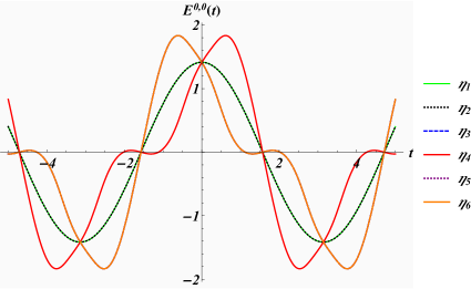
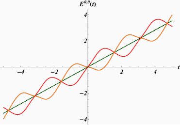
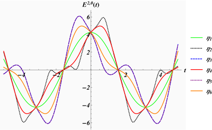
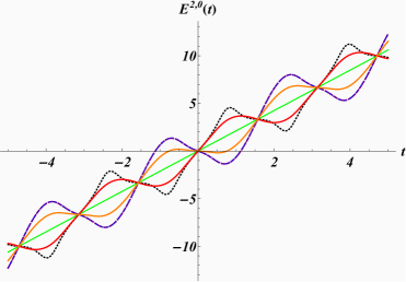
Figure 1: The instantaneous energy spectra (72) associated with the six Dyson maps for $\lambda(t)=\sin(2t)$ for case 1 with $c_{+}=c_{-}=1$, $k_{1}=2$. In panels (a), (c) we have $a(t)=\cos(t)$ and in panels (a), (c) we that $a(t)=t/2$.

For concrete choices of the time-dependent coefficient functions we can now directly evaluate the expressions for $E_{i}^{n,m}(t)$ corresponding to the Dyson maps $\eta_{i}(t)$ explicitly by computing the auxiliary functions $\chi(t)$ and the functions $f_{i}(t)$. The Dyson map $\eta_{2}$ leads to somewhat different behaviour. This is understood by the fact that it can only be constructed at $c=0$ and at what would be the exceptional point in the time-independent scenario $c=\lambda$. Hence also the energies exhibit slightly different characteristics. Taking the above mentioned constraints into account there are large regions in the parameter space for which the all ot the energies $E_{i}^{n,m}(t)$ are real and hence physical. We illustrate the behaviour of these energies for each of the Dyson maps in figues 1 and 2 for some concrete choices.

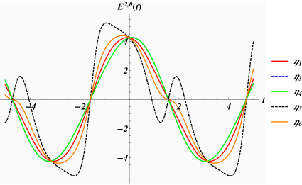
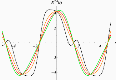
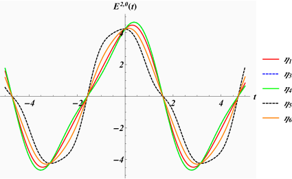
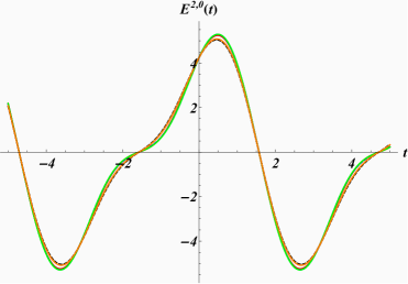
Figure 2: The instantaneous energy spectra (72) associated with five Dyson maps for $\lambda(t)=\sin(2t)$, $a(t)=\cos(t)$ for case 2 with $c_{+}=c_{-}=1$, $k_{1}=2.5$, $k_{2}=1$. We have $p=-0.1$, $p=-0.3$, $p=-0.5$, $p=-0.9$ in panels (a), (b), (c), (d), respectively.

First of all we observe from figure 1 the crucial feature that the instantaneous energy is real and finite. Secondly we note that despite sharing the same non-Hermitian Hamiltonian, the theories related to different Dyson maps can lead to quite different physical behaviour in the energy. Similar to the time-independent scenario, this is the known fact that the Hamiltonian alone does not define a unique definite physical system, but to define the physics one also needs to specify the metric, i.e. the Dyson map. We note that some of the energies can become degenerate, $E_{1}^{n,n}=E_{2}^{n,n}$, which can however split when $n\neq m$. As is also expected from the explicit expressions, the differences are more amplified the larger $\left|n-m\right|$. In case 2, when we have non vanishing values of the parameter $p$ these effects are even more amplified as can be seen in figure 2. We notice a strong sensitivity with regard to $p$.

The constraints resulting from the parameterization, $\left|p\right|<1$, imply that we are in the regime with spontaneously broken $\mathcal{PT}$-symmetry when compared to the time-independent case. Therefore, we observe the same phenomenon that was first noted in [20, 26], namely that the introduction of a time-dependence into the metric will mend the spontaneously broken $\mathcal{PT}$-regime so that it becomes physically meaningful. In this case this manifests itself by the fact that the instantaneous energy is real.

3.2 Metric and Dyson maps with $\mu(t)\neq 0$, case 3

Finally we also discuss the case 3 by including a Hermitian coupling term into the Hamiltonian in addition to the non-Hermitian one. This case turns out to be more complicated to solve, but may also be tackled successfully by our perturbative method. Keeping the expression (14) as our Ansatz for the perturbative expansion for the metric we obtain the same first order equation (15), but now involving

$$h_{0}(t)=a(t)\left(K_{1}+K_{2}\right)+\mu(t)K_{4}\qquad\text{and}\qquad h_{1}(t)=\lambda(t)K_{3}.$$ (73)

Since all generators of the algebra commute with $K_{1}+K_{2}$ the only nontrivial contribution in the commutator of that relation results from the term involving $K_{4}$ in $h_{0}$. Taking now

$$q_{1}=K_{1},\qquad q_{2}=K_{2},\qquad q_{3}=K_{3},$$ (74)

leads to the following first order equations for the time-dependent coefficient functions

$$\dot{\gamma}_{1}^{(1)}(t)=-\frac{1}{2}\mu(t)\gamma_{3}^{(1)}(t),$$ (75)

$$\dot{\gamma}_{2}^{(1)}(t)=\frac{1}{2}\mu(t)\gamma_{3}^{(1)}(t),$$ (76)

$$\dot{\gamma}_{3}^{(1)}(t)=\mu(t)\left[\gamma_{1}^{(1)}(t)-\gamma_{2}^{(1)}(t)\right]-\lambda(t).$$ (77)

We see immediately that $\gamma_{2}^{(1)}(t)=-\gamma_{1}^{(1)}(t)$, which then also simplifies equations (77).

Proceeding now in the same manner as in the previous cases by extrapolation to the full series, we find that the following two equations need to be satisfied

$$\dot{\gamma}_{1}(t)=-\frac{1}{2}\sinh[\gamma_{3}(t)]\mu(t)\qquad\text{and}\qquad\dot{\gamma}_{3}(t)=\cosh[\gamma_{3}(t)]\tanh[2\gamma_{1}(t)]\mu(t)-\lambda(t).$$ (78)

Letting $\lambda=p\mu$, we can express $\gamma_{3}$ as a function of $\gamma_{1}$

$$\gamma_{3}(\gamma_{1})=\pm\mathop{\mathrm{a}rccosh}\left[p\tanh(2\gamma_{1})-\frac{k_{1}}{2}\mathop{\mathrm{s}ech}(2\gamma_{1})\right].$$ (79)

Setting

$$\gamma_{1}=\frac{1}{2}\mathop{\mathrm{a}rcsinh}(\chi),$$ (80)

the two first order equations (78) are converted into the linear second order auxiliary equation (46) with $\lambda\rightarrow\mu$. The resulting Hermitian Hamiltonian consists now not only of two decoupled harmonic oscillators, but also contains an additional Hermitian term in form of $K_{4}$

$$h(t)=a(t)\left(K_{1}+K_{2}\right)-\frac{k_{1}+2p\chi(t)}{2\left[1+\chi(t)^{2}\right]}\mu(t)K_{4}.$$ (81)

As in the previous two cases, we may also construct a non-Hermitian solution for the Dyson map by means of the perturbative approach. From the first order equation we observe that also $q_{3}=iK_{4}$ with $q_{1}$ and $q_{2}$ as in (74) leads to a solution. Extrapolating to all orders yields now the two equations

$$\dot{\gamma}_{1}(t)=-\frac{1}{2}\sin[\gamma_{3}(t)]\lambda(t)\qquad\text{and}\qquad\dot{\gamma}_{3}(t)=\mu(t)-\cos[\gamma_{3}(t)]\coth[2\gamma_{1}(t)]\lambda(t).$$ (82)

As before we must restrict $\lambda(t)=p\mu(t)$ so that we may solve for $\gamma_{3}$ in terms of $\gamma_{1}$

$$\gamma_{3}(\gamma_{1})=\pm\arccos\left\{\frac{\left[2-ik_{2}+2\cosh\left(2\gamma_{1}\right)\right]\mathop{\mathrm{c}sch}(2\gamma_{1})}{2p}\right\}.$$ (83)

We set here $k_{2}=0$ in order to obtain a real solution. Letting now

$$\gamma_{1}=\frac{1}{2}\mathop{\mathrm{a}rccosh}(\chi),$$ (84)

the two first order equations (82) are now converted into the linear second order auxiliary equation (46) with $\lambda\rightarrow\mu$ and $k_{1}\rightarrow 0$. Similarly as the resulting Hamiltonian for the Hermitian Dyson map the resulting Hermitian Hamiltonian contain a $K_{4}$ besides the two uncoupled harmonic oscillators

$$h(t)=a(t)\left(K_{1}+K_{2}\right)+\frac{\mu(t)}{\chi(t)-1}K_{4}.$$ (85)

The generator $K_{4}$ can be identified with the standard angular momentum operator $L_{z}$ and can be eliminated from $h(t)$ in (81) and (85) by means of a unitary transformation, see for instance [37]. Subsequently the eigenfunctions and expectation values of the resulting system of two uncoupled harmonic oscillators can be obtained similarly as for the cases $1$ and $2$ presented in detail in the previous section.

4 The unstable anharmonic quartic oscillator

In this section we discuss an example for which the previous versions of the perturbative expressions for the metric or the Dyson map do not however lead to any solution. In fact, as we will demonstrate one does not only have to change the Ansatz, but one also needs to rescale the Hamiltonian in order to introduce the perturbative parameter in the right terms and treat the non-Hermitian part as a strong rather than a weak perturbation.

Unstable anharmonic oscillators have been the testing ground for perturbative methods for nonlinear systems for more than fifty years [38, 39, 40, 41, 42]. Only fairly recently an exact solution for the time-independent unstable anharmonic quartic oscillator was found by Jones and Mateo [43]. They used ideas from non-Hermitian $\mathcal{PT}$-symmetric quantum mechanics [44, 4] and applied a perturbative approach that turned out to be exact. Recently we [24] also solved the explicitly time-dependent version of this model in an exact manner. These exact solutions found in [24] will serve here as a benchmark for our perturbative approach, so that we consider the same Hamiltonian, but with the time-dependent mass term set to zero

$$H(z,t)=p^{2}-\frac{g(t)}{16}z^{4},~{}~{}~{}~{}~{}g\in\mathbb{R}^{+}\text{.}$$ (86)

Defining $H(z,t)$ on the contour $z=-2i\sqrt{1+ix}$ as proposed in [43], it is mapped into the non-Hermitian Hamiltonian

$$H(x,t)=p^{2}-\frac{1}{2}p+\frac{i}{2}\{x,p^{2}\}+g(t)(x-i)^{2},$$ (87)

where $\{\cdot,\cdot\}$ denotes as usual the anti-commutator. As mentioned using our previous versions for the perturbative Ansatz does not lead to a solvable first order equation or a recursive system. Instead we change our Ansatz to

$$\rho(t)=\eta(t)^{\dagger}\eta(t)=\prod_{i=j}^{1}\left[\prod_{l=k}^{1}\exp\left(\epsilon^{-l}(\gamma_{i}^{(l)})^{\dagger}q_{i}\right)\right]\prod_{i=1}^{j}\left[\prod_{l=1}^{k}\exp\left(\epsilon^{-l}(\gamma_{i}^{(l)})q_{i}\right)\right].$$ (88)

As we are expanding in $\epsilon^{-1}$ we assume here that perturbation parameter, $\epsilon\gg 1$, is large. The reason for this is that in addition we also need to scale the Hamiltonian (87) as $x\rightarrow\epsilon x$. Separating now into a Hermitian and non-Hermitian term, $h_{0}(t)$ and $h_{p}(t)$, respectively, we have

$$h_{0}(t)=p^{2}-\frac{1}{2}p+\epsilon^{2}g(t)x^{2}-g(t),\qquad\text{and}\qquad h_{p}(t)=-2i\epsilon g(t)x+\frac{1}{2}i\epsilon\{x,p^{2}\}.$$ (89)

Thus instead of adding a small non-Hermitian perturbation to the Hermitian part, we have perturbed by a large term and also scaled up the harmonic oscillator term. Our Hamiltonian acquires therefore the following generic form

$$H(t)=h_{1}(t)+\epsilon^{2}h_{2}(t)+i\epsilon h_{3}(t),$$ (90)

which together with the Ansatz (88) leads to the new first order equation

$$2ih_{3}(t)+\sum_{i=1}^{j}\left[\left((\gamma_{i}^{(1)}+(\gamma_{i}^{(1)})^{\dagger}\right)\left[q_{i},h_{2}(t)\right]\right]=0.$$ (91)

From this equation we can see that if any of the time-dependent coefficient functions $\gamma_{i}^{(1)}$’s are purely imaginary, then their contributions vanishes at this order and if they are real we simply acquire a factor of 2. This version of the Ansatz leads to a recursive system that can be solved systematically order by order. In our example for the Hamiltonian (87) we identify

$$h_{3}(t)=h_{p}(t)\qquad\text{and}\qquad h_{2}(t)=g(t)x^{2},$$ (92)

and may satisfy the lowest order equation with the choice

$$q_{1}=x,\qquad q_{2}=p^{2},\qquad q_{3}=p^{2},\qquad q_{4}=p,$$ (93)

where for $q_{3}$ and $q_{4}$ we are taking their time-dependent coefficient functions to be purely imaginary. In doing so we end up with following equations that need to be satisfied

$$\gamma_{2}^{(1)}=\frac{1}{6g},\qquad\text{and}\qquad\gamma_{3}^{(0)}=\frac{1}{2\gamma_{1}^{(1)}}.$$ (94)

At order $\epsilon^{0}$ we read off the constraining equations

$$\gamma_{2}^{(2)}=0\qquad\text{and}\qquad\gamma_{1}^{(2)}=-2\left(\gamma_{1}^{(1)}\right)^{2}\gamma_{3}^{(1)}.$$ (95)

Continuing to order $\epsilon^{-1}$ we find the constraints

$$\gamma_{1}^{(1)}=\frac{\dot{g}}{6g},~{}~{}\gamma_{1}^{(3)}=-\frac{\gamma_{3}^{(2)}\dot{g}^{2}}{18g^{2}}+\frac{\dot{g}^{3}}{72g^{4}}+\frac{\left(\gamma_{3}^{(1)}\right)^{2}\dot{g}^{3}}{54g^{3}}-\frac{\dot{g}\ddot{g}}{72g^{3}},~{}~{}\dot{\gamma}_{4}^{(0)}+\gamma_{4}^{(0)}\left(\frac{\ddot{g}}{\dot{g}}-\frac{\dot{g}}{g}\right)=-\frac{1}{3}.$$ (96)

The last equation is solved to

$$\gamma_{4}^{(0)}=\frac{c_{1}g}{\dot{g}}-\frac{g\log{g}}{2\dot{g}}.$$ (97)

At order $\epsilon^{-2}$ we obtain $\gamma_{3}^{(1)}=0$, and therefore with (95) we have $\gamma_{1}^{(2)}=0$.

At order $\epsilon^{-3}$ we obtain

$$\gamma_{3}^{(2)}=\frac{\dot{g}^{2}-g\ddot{g}}{4g^{2}\dot{g}},$$ (98)

which implies with (96) that $\gamma_{1}^{(3)}=0$. Some features hold for all remaining orders in $\varepsilon$. We have $\gamma_{2}^{(i)}=0$ for all $i\geq 2$. We also find that at every order $\epsilon^{-n}$, where $n\geq 2$ the differential equation

$$\frac{\gamma_{4}^{(n-1)}\dot{g}^{2}}{3g^{2}}+\frac{\dot{g}\dot{\gamma}_{4}^{(n-1)}}{3g}+\frac{\gamma_{4}^{(n-1)}\ddot{g}}{3g}=0,$$ (99)

occurs, which is solved by

$$\gamma_{4}^{(n-1)}=\frac{c_{n-1}g}{\dot{g}}$$ (100)

Another equation that appears at all orders $\epsilon^{-n}$ for $n\geq 2$ is given by

$$\gamma_{1}^{(n+2)}=-\frac{\gamma_{3}^{(n+1)}\dot{g}^{2}}{18g^{2}}$$ (101)

This is solved at all orders if we have

$$\gamma_{1}^{(n+2)}=0\qquad\text{and}\qquad\gamma_{3}^{(n+1)}=0$$ (102)

for $n\geq 2$. When eliminating the $\gamma$s from these equations we are left with a differential equation entirely in $g$ given by

$$\frac{14\dot{g}^{3}}{9g^{2}}+\frac{2\dot{g}\ddot{g}}{g}-\frac{\dddot{g}}{2}=0$$ (103)

Parameterizing $g=\frac{1}{2}\sigma^{-3}$ this equation reduces to

$$\sigma^{2}\dddot{\sigma}=0$$ (104)

which is easily solved by $\sigma(t)=c_{1}+c_{2}t+c_{3}t^{2}$.

Assembling all our results we extrapote to all orders, i.e. an exact solution. Setting therefore $\varepsilon=1$ gives the time-dependent Dyson map of the form

$$\eta(t)=\exp[\gamma_{1}(t)x]\exp[\gamma_{2}(t)p^{3}+i\gamma_{3}(t)p^{2}+i\gamma_{4}(t)p],$$ (105)

with

$$\gamma_{1}=\frac{\dot{g}}{6g},\quad\gamma_{2}=\frac{1}{6g},\quad\gamma_{3}=\frac{12g^{3}+\dot{g}^{2}-g\ddot{g}}{4\dot{g}g^{2}},\quad\gamma_{4}=\frac{g}{\dot{g}}\left(c_{1}-\frac{\log{g}}{2}\right),$$ (106)

which is in precise agreement with the Dyson map we previously found in [24].

5 Conclusions

We have demonstrated how to set up a perturbative approach that allows to construct the metric operator and the Dyson map in a recursive manner order by order in a perturbative parameter that may be very small or very large. We found three different types of perturbative expansions. The Ansatz (12) is the most natural one when the Dyson map is assumed to be Hermitian and needs to be slightly modified when one allows $\eta$ to be non-Hermitian as shown in section 3.1.2. In both of these versions the non-Hermitian term was treated as a small perturbation. In section 4 we demonstrated that this approach can not be applied universally and has to be altered for some models for which one needs to treat the non-Hermitian term and parts of the Hermitian term as large perturbations. Consequently the perturbative expansion needs to be in the inverse of the large perturbative parameter.

When compared to the time-independent scenario, all our approaches have in common that the order-by-order equations do not just determine the commutative structure of the $q_{i}$s, but computations are more involved as in addition one needs to solve coupled sets of differential equations for the time-dependent coefficient functions. Moreover, we observed that the key structure is already determined by the lowest order equation.

Although the main emphasis in this paper is on the perturbation theory, with regard to the specific example studied we found many new Dyson maps for the coupled non-Hermitian harmonic oscillator. We saw that these different maps lead to different types of physical behaviour, as shown explicitly for the time-dependent energy expectation values. When compared to the time-independent case, all our solutions are only valid in what would be the spontaneously broken $\mathcal{PT}$-regime, except for one example that is defined on what would be the exceptional point. So similar to the effect observed in [20, 26], this regime becomes physically meaningful in the time-dependent setting. However, unlike as in some of the previously studied systems, one can not crossover to the $\mathcal{PT}$-regime and is confined to the broken phase. It remains an open issue to formulate general criteria that characterize precisely when this possibility occurs for time-dependent systems and when not.

Acknowledgments: RT is supported by a City, University of London Research Fellowship.

References

- [1] C. M. Bender and S. Boettcher, Real spectra in non-hermitian hamiltonians having PT symmetry, Physical Review Letters 80(24), 5243–5246 (1998).
- [2] C. M. Bender, Making sense of non-Hermitian Hamiltonians, Reports on Progress in Physics 70(6), 947–1018 (2007).
- [3] A. Mostafazadeh, Pseudo-Hermitian representation of quantum mechanics, International Journal of Geometric Methods in Modern Physics 7(7), 1191–1306 (2010).
- [4] C. M. Bender, P. E. Dorey, C. Dunning, A. Fring, D. W. Hook, H. F. Jones, S. Kuzhel, G. Levai, and R. Tateo, PT Symmetry: In Quantum and Classical Physics, (World Scientific, Singapore) (2019).
- [5] H. F. Jones and J. Mateo, Equivalent Hermitian Hamiltonian for the non-Hermitian -x4 potential, Physical Review D - Particles, Fields, Gravitation and Cosmology 73(8) (2006).
- [6] P. E. Assis and A. Fring, Metrics and isospectral partners for the most generic cubic PT -symmetric non-Hermitian Hamiltonian, Journal of Physics A: Mathematical and Theoretical 41(24) (2008).
- [7] P. E. Assis and A. Fring, Non-Hermitian Hamiltonians of Lie algebraic type, Journal of Physics A: Mathematical and Theoretical 42(1) (2009).
- [8] A. Mostafazadeh, Metric operators for quasi-Hermitian Hamiltonians and symmetries of equivalent Hermitian Hamiltonians, Journal of Physics A: Mathematical and Theoretical 41(24) (2008).
- [9] D. P. Musumbu, H. B. Geyer, and W. D. Heiss, Choice of a metric for the non-Hermitian oscillator, J. Phys. A40, F75–F80 (2007).
- [10] C. M. Bender, D. C. Brody, and H. F. Jones, Complex Extension of Quantum Mechanics, Physical Review Letters 89(27) (2002).
- [11] P. Siegl and D. Krejčiřík, On the metric operator for the imaginary cubic oscillator, Physical Review D - Particles, Fields, Gravitation and Cosmology 86(12) (2012).
- [12] C. Figueira De Morisson Faria and A. Fring, Time evolution of non-Hermitian Hamiltonian systems, Journal of Physics A: Mathematical and General 39(29), 9269–9289 (2006).
- [13] A. Mostafazadeh, Time-dependent pseudo-Hermitian Hamiltonians defining a unitary quantum system and uniqueness of the metric operator, Physics Letters, Section B: Nuclear, Elementary Particle and High-Energy Physics 650(2-3), 208–212 (2007).
- [14] M. Znojil, Time-dependent version of crypto-Hermitian quantum theory, Physical Review D - Particles, Fields, Gravitation and Cosmology 78(8) (2008).
- [15] H. Bíla, Adiabatic time-dependent metrics in PT-symmetric quantum theories, arXiv preprint arXiv:0902.0474 (2009).
- [16] J. Gong and Q.-H. Wang, Time-dependent PT-symmetric quantum mechanics, J. Phys. A: Math. and Theor. 46(48), 485302 (2013).
- [17] A. Fring and M. H. Moussa, Non-Hermitian Swanson model with a time-dependent metric, Physical Review A 94(4) (2016).
- [18] M. Maamache, O. Kaltoum Djeghiour, N. Mana, and W. Koussa, Pseudo-invariants theory and real phases for systems with non-Hermitian time-dependent Hamiltonians, European Physical Journal Plus 132(9) (2017).
- [19] A. Fring and M. H. Moussa, Unitary quantum evolution for time-dependent quasi-Hermitian systems with nonobservable Hamiltonians, Physical Review A 93(4) (2016).
- [20] A. Fring and T. Frith, Mending the broken PT-regime via an explicit time-dependent Dyson map, Physics Letters, Section A: General, Atomic and Solid State Physics 381(29), 2318–2323 (2017).
- [21] A. Fring and T. Frith, Exact analytical solutions for time-dependent Hermitian Hamiltonian systems from static unobservable non-Hermitian Hamiltonians, Physical Review A 95(1) (2017).
- [22] A. Fring and T. Frith, Metric versus observable operator representation, higher spin models, European Physical Journal Plus 133(2) (2018).
- [23] D.-J. Zhang, Q.-H. Wang, and J. Gong, Time-dependent PT-symmetric quantum mechanics in generic non-Hermitian systems, Phys. Rev. A 100(6), 062121 (2019).
- [24] A. Fring and R. Tenney, Spectrally equivalent time-dependent double wells and unstable anharmonic oscillators, Phys. Lett. A , 126530 (2020).
- [25] H. R. Lewis and W. B. Riesenfeld, An exact quantum theory of the time-dependent harmonic oscillator and of a charged particle in a time-dependent electromagnetic field, Journal of Mathematical Physics 10(8), 1458–1473 (1969).
- [26] A. Fring and T. Frith, Solvable two-dimensional time-dependent non-Hermitian quantum systems with infinite dimensional Hilbert space in the broken PT-regime, Journal of Physics A: Mathematical and Theoretical 51(26) (2018).
- [27] A. Fring and T. Frith, Time-dependent metric for the two-dimensional, non-Hermitian coupled oscillator, Modern Physics Letters A (2019).
- [28] A. Fring and T. Frith, Mending the broken PT-regime via an explicit time-dependent Dyson map, Physics Letters, Section A: General, Atomic and Solid State Physics 381(29), 2318–2323 (2017).
- [29] A. Fring and T. Frith, Eternal life of entropy in non-Hermitian quantum systems, Physical Review A 100(1) (2019).
- [30] T. Frith, Exotic entanglement for non-Hermitian Jaynes-Cummings Hamiltonians, arXiv preprint arXiv:2006.09909 (2020).
- [31] J. Cen and A. Saxena, Anti-PT-symmetric Qubit: Decoherence and Entanglement Entropy, arXiv preprint arXiv:2008.04514 (2020).
- [32] C. M. Bender, D. C. Brody, and H. F. Jones, Extension of PT-symmetric quantum mechanics to quantum field theory with cubic interaction, Physical Review D - Particles, Fields, Gravitation and Cosmology 70(2) (2004).
- [33] A. Mostafazadeh, -symmetric cubic anharmonic oscillator as a physical model, J. of Phys. A: Mathematical and General 38(29), 6557 (2005).
- [34] V. P. Ermakov, Transformation of differential equations, Univ. Izv. Kiev. 20, 1 (1880).
- [35] E. Pinney, The nonlinear differential equation y”(x) + p(x) y +c/y^3 = 0, Proc. Amer. Math. Soc 681(1) (1950).
- [36] I. A. Pedrosa, Exact wave functions of a harmonic oscillator with time-dependent mass and frequency, Physical Review A - Atomic, Molecular, and Optical Physics 55(4), 3219–3221 (1997).
- [37] M. Maamache, A. Bounames, and N. Ferkous, Comment on ’Wave functions of a time-dependent harmonic oscillator in a static magnetic field’, Phys. Rev. A 73, 016101 (2006).
- [38] C. M. Bender and T. T. Wu, Anharmonic oscillator, Phys. Rev. 184(5), 1231 (1969).
- [39] A. A. Andrianov, The large N expansion as a local perturbation theory, Annals of Physics 140(1), 82–100 (1982).
- [40] S. Graffi and V. Grecchi, The Borel sum of the double-well perturbation series and the Zinn-Justin conjecture, Phys. Lett. B 121(6), 410–414 (1983).
- [41] E. Caliceti, V. Grecchi, and M. Maioli, Double wells: perturbation series summable to the eigenvalues and directly computable approximations, Comm. Math. Phys. 113(4), 625–648 (1988).
- [42] V. Buslaev and V. Grecchi, Equivalence of unstable anharmonic oscillators and double wells, J. of Phys. A: Math. and Gen. 26(20), 5541 (1993).
- [43] H. F. Jones and J. Mateo, An Equivalent Hermitian Hamiltonian for the non-Hermitian Potential, Phys. Rev. D73, 085002 (2006).
- [44] A. Mostafazadeh, Pseudo-Hermitian Representation of Quantum Mechanics, Int. J. Geom. Meth. Mod. Phys. 7, 1191–1306 (2010).