TimeAutoML: Autonomous Representation Learning for Multivariate Irregularly Sampled Time Series

Abstract

Multivariate time series (MTS) data are becoming increasingly ubiquitous in diverse domains, e.g., IoT systems, health informatics, and 5G networks. To obtain an effective representation of MTS data, it is not only essential to consider unpredictable dynamics and highly variable lengths of these data but also important to address the irregularities in the sampling rates of MTS. Existing parametric approaches rely on manual hyperparameter tuning and may cost a huge amount of labor effort. Therefore, it is desirable to learn the representation automatically and efficiently. To this end, we propose an autonomous representation learning approach for multivariate time series (TimeAutoML) with irregular sampling rates and variable lengths. As opposed to previous works, we first present a representation learning pipeline in which the configuration and hyperparameter optimization are fully automatic and can be tailored for various tasks, e.g., anomaly detection, clustering, etc. Next, a negative sample generation approach and an auxiliary classification task are developed and integrated within TimeAutoML to enhance its representation capability. Extensive empirical studies on real-world datasets demonstrate that the proposed TimeAutoML outperforms competing approaches on various tasks by a large margin. In fact, it achieves the best anomaly detection performance among all comparison algorithms on 78 out of all 85 UCR datasets, acquiring up to 20% performance improvement in terms of AUC score.

1 Introduction

The past decade has witnessed a rising proliferation in Multivariate Time Series (MTS) data, along with a plethora of applications in domains as diverse as IoT data analysis, medical informatics, and network security. Given the huge amount of MTS data, it is crucial to learn their representations effectively so as to facilitate underlying applications such as clustering and anomaly detection. For this purpose, different types of methods have been developed to represent time series data.

Traditional time series representation techniques, e.g., Discrete Fourier Transform (DCT) (Faloutsos et al., 1994), Discrete Wavelet Transform (DWT)(Chan & Fu, 1999), Piecewise Aggregate Approximation (PAA)(Keogh et al., 2001), etc., represent raw time series data based on specific domain knowledge/data properties and hence could be suboptimal for subsequent tasks given the fact that their objectives and feature extraction are decoupled.

More recent time series representation approaches, e.g., Deep Temporal Clustering Representation (DTCR) (Ma et al., 2019), Self-Organizing Map based Variational Auto Encoder (SOM-VAE) (Fortuin et al., 2018), etc., optimize the representation and the underlying task such as clustering in an end-to-end manner. These methods usually assume that time series under investigation are uniformly sampled with a fixed interval. This assumption, however, does not always hold in many applications. For example, within a multimodal IoT system, the sampling rates could vary for different types of sensors.

Unsupervised representation learning for irregularly sampled multivariate time series is a challenging task and there are several major hurdles preventing us from building effective models: i) the design of neural network architecture often employs a trial and error procedure which is time consuming and could cost a substantial amount of labor effort; ii) the irregularity in the sampling rates constitutes a major challenge against effective learning of time series representations and render most existing methods not directly applicable; iii) traditional unsupervised time series representation learning approach does not consider contrastive loss functions and consequently only can achieve suboptimal performance.

To tackle the aforementioned challenges, we propose an autonomous unsupervised representation learning approach for multivariate time series to represent irregularly sampled multivariate time series. TimeAutoML differs from traditional time series representation approaches in three aspects. First, the representation learning pipeline configuration and hyperparameter optimization are carried out automatically. Second, a negative sample generation approach is proposed to generate negative samples for contrastive learning. Finally, an auxiliary classification task is developed to distinguish normal time series from negative samples. In this way, the representation capability of TimeAutoML is greatly enhanced. We conduct extensive experiments on UCR time series datasets and UEA multivariate time series datasets. Our experiments demonstrate that the proposed TimeAutoML outperforms comparison algorithms on both clustering and anomaly detection tasks by a large margin, especially when time series data is irregularly sampled.

2 Related Work

Unsupervised Time Series Representation Learning

Time series representation learning plays an essential role in a multitude of downstream analysis such as classification, clustering, anomaly detection. There is a growing interest in unsupervised time series representation learning, partially because no labels are required in the learning process, which suits very well many practical applications. Unsupervised time series representation learning can be broadly divided into two categories, namely 1) multi-stage methods and 2) end-to-end methods. Multi-stage methods first learn a distance metric from a set of time series, or extract the features from the time series, and then perform downstream machine learning tasks based on the learned or the extracted features. Euclidean distance (ED) and Dynamic Time Warping (DTW) are the most commonly used traditional time series distance metrics. Although the ED is competitive, it is very sensitive to outliers in the time series. The main drawback of DTW is its heavy computational burden. Traditional time series feature extraction methods include Singular Value Decomposition (SVD), Symbolic Aggregate Approximation (SAX), Discrete Wavelet Transform (DWT)(Chan & Fu, 1999), Piecewise Aggregate Approximation (PAA)(Keogh et al., 2001), etc. Nevertheless, most of these traditional methods are for regularly sampled time series, so they may not perform well on irregularly sampled time series. In recent years, many new feature extraction methods and distance metrics are proposed to overcome the drawbacks mentioned above. For instance, Paparrizos & Gravano (2015); Petitjean et al. (2011) combine the proposed distance metrics and K-Means algorithm to achieve clustering. Lei et al. (2019) first extracts sparse features of time series, which is not sensitive to outliers and irregular sampling rate, and then carries out the K-Means clustering. In contrast, end-to-end approaches learn the representation of the time series in an end-to-end manner without explicit feature extraction or distance learning (Fortuin et al., 2018; Ma et al., 2019). However, the aforementioned methods need to manually design the network architecture based on human experience which is time-consuming and costly. Instead, we propose in this paper a representation learning method which optimizes an AutoML pipeline and their hyperparameters in a fully autonomous manner. Furthermore, we consider negative sampling and contrastive learning in the proposed framework to effectively enhance the representation ability of the proposed neural network architecture.

Irregularly Sampled Time Series Learning

There exist two main groups of works regarding machine learning for irregularly sampled time series data. The first type of methods impute the missing values before conducting the subsequent machine learning tasks (Shukla & Marlin, 2019; Luo et al., 2018; 2019; Kim & Chi, 2018). The second type directly learns from the irregularly sampled time series. For instance, Che et al. (2018); Cao et al. (2018) propose a memory decay mechanism, which replaces the memory cell of RNN by the memory of the previous timestamp multiplied by a learnable decay coefficient when there are no sampling value at this timestamp. Rubanova et al. (2019) combines RNN with ordinary differential equation to model the dynamic of irregularly sampled time series. Different from the previous works, TimeAutoML makes use of the special characteristics of RNN (Abid & Zou, 2018) and automatically configure a representation learning pipeline to model the temporal dynamics of time series.

AutoML

Automatic Machine Learning (AutoML) aims to automate the time-consuming model development process and has received significant amount of research interests recently. Previous works about AutoML mostly emphasize on the domains of computer vision and natural language processing, including object detection (Ghiasi et al., 2019; Xu et al., 2019; Chen et al., ), semantic segmentation (Weng et al., 2019; Nekrasov et al., 2019; Bae et al., 2019), translation (Fan et al., 2020) and sequence labeling (Chen et al., 2018a). However, AutoML for time series learning is an underappreciated topic so far and the existing works mainly focus on supervised learning tasks, e.g., time series classification. Ukil & Bandyopadhyay propose an AutoML pipeline for automatic feature extraction and feature selection for time series classification. van Kuppevelt et al. (2020) develops an AutoML framework for supervised time series classification, which involves both neural architecture search and hyperparameter optimization. Olsavszky et al. (2020) proposes a framework called AutoTS, which performs time series forecasting of multiple diseases. Nevertheless, to our best knowledge, no previous work has addressed unsupervised time series learning based on AutoML.

Summary of comparisons with related work

We next provide a comprehensive comparison between the proposed framework and other state-of-the-art methods, including (WaRTEm (Mathew et al., 2019), DTCR (Ma et al., 2019), USRLT (Franceschi et al., 2019) and BeatGAN (Zhou et al., 2019)), as shown in Table 1. In particular, we emphasize on a total of seven features in the comparison, including data augmentation, negative sample generation, contrastive learning, selection of autoencoders, similarity metric selection, attention mechanism selection, and automatic hyperparameter search. TimeAutoML is the only method that has all the desired properties.

Table 1: Comparisons with related methods

	WaRTEm	DTCR	USRLT	BeatGAN	TimeAutoML
Data augmentation				✓	✓
Negative sample generation	✓	✓	✓		✓
Contrastive training	✓	✓	✓		✓
Autoencoder selection					✓
Similarity metric selection					✓
Attention mechanism selection					✓
Automatic hyperparameter search					✓

3 TimeAutoML Framework

3.1 Proposed AutoML Framework

Let $\bm{X}=\{\underline{\bm{x}}_{1},\underline{\bm{x}}_{2},\cdots\underline{\bm{x}}_{N}\}$ denote a set of $N$ time series in which $\underline{\bm{x}}_{i}\in{\mathbb{R}^{{T_{i}}}}$, where ${T_{i}}$ is the length of the $i^{th}$ time series $\underline{\bm{x}}_{i}$. We aim to build an automated time series representation learning framework to generate task-aware representations that can support a variety of downstream machine learning tasks. In addition, we consider negative sample generation and contrastive self-supervised learning. The contrastive loss function focuses on building time series representations by learning to encode what makes two time series similar or different. The proposed TimeAutoML framework can automatically configure an representation learning pipeline with an array of functional modules, each of these modules is associated with a set of hyperparameters. We assume there are a total of $M$ modules and there are ${Q_{i}}$ options for the $i^{th}$ functional module. Let ${\bm{\underline{k}}_{i}}\in{\{0,1\}^{{Q_{i}}}}$ denote an indicating vector for $i^{th}$ module, with the constraint ${1^{\top}}{\bm{\underline{k}}_{i}}{\rm{=}}\sum\nolimits_{j=1}^{{Q_{i}}}{{k_{i,j}}}=1$ ensuring that only a single option is chosen for each module. Let $\bm{\underline{\theta}}_{i,j}$ be the hyperparameters of $j^{th}$ option in $i^{th}$ module, where $\bm{\underline{\theta}}_{i,j}^{C}$ and $\bm{\underline{\theta}}_{i,j}^{D}$ are respectively the continuous and discrete hyperparameters. Let $\Theta$ and ${\rm K}$ denote the set of variables to optimize, i.e., $\Theta=\{{\bm{\underline{\theta}}_{i,j}},\forall i\in[M],j\in[{Q_{i}}]\}$ and ${\rm K}=\{\bm{\underline{k}}_{1},\ldots,\bm{\underline{k}}_{M}\}$. We further let $f({\rm K},\Theta)$ denote the corresponding objective function value. Please note that the objective function differs for different tasks. For anomaly detection, we use Area Under the Receiver Operating Curve (AUC) as objective function while we use the Normalized Mutual Information (NMI) as objective function for clustering. The optimization problem of automatic pipeline configuration is shown below.

$$\begin{array}[]{l}\mathop{\max}\limits_{{\rm K},\Theta}f({\rm K},\Theta)\\ \text{subject\ to}\left\{\begin{array}[]{l}{\bm{\underline{k}}_{i}}\in{\{0,1\}^{{Q_{i}}}},{1^{\top}}{\bm{\underline{k}}_{i}}=1,\forall i\in[M],\\ \bm{\underline{\theta}}_{i,j}^{C}\in C_{i,j},\bm{\underline{\theta}}_{i,j}^{D}\in D_{i,j},\forall i\in[M],j\in[{Q_{i}}].\end{array}\right.\end{array}$$ (1)

We solve problem (1) by alternatively leveraging Thompson sampling and Bayesian optimization, which will be discussed as follows.

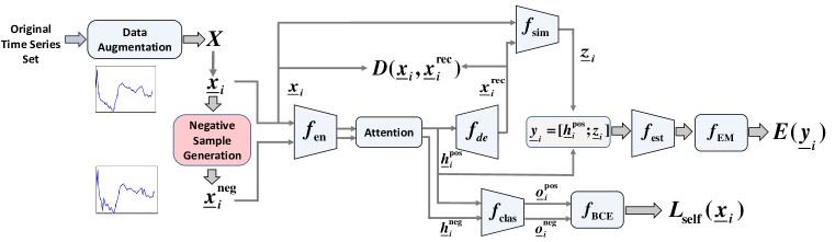
Figure 1: TimeAutoML pipeline.

3.1.1 Pipeline Configuration

We first assume that the hyperparameters $\Theta$ are fixed during the pipeline configuration. We aim at selecting the better module option ${\rm K}$ to optimize objective function $f({\rm K},\Theta)$, we can delineate it as a ${\rm K}-\max$ problem:

$$\begin{array}[]{l}{\rm K}=\mathop{\max}\limits_{\rm K}f({\rm K},\Theta)+{\chi_{K}}({\rm K}),\quad{\chi_{K}}({\rm K})=\left\{\begin{array}[]{l}0,\quad\text{if}\ {\rm K}\in K\\ -\infty,\quad\text{else}\end{array},\right.\end{array}$$ (2)

where $K$ is the feasible set, i.e., $K=\{{\rm K}:{\rm K}=\{{\bm{\underline{k}}_{i}}\},{\bm{\underline{k}}_{i}}\in{\{0,1\}^{{Q_{i}}}},{1^{\top}}{\bm{\underline{k}}_{i}}=1,\forall i\in[M]\}$ and ${\chi_{K}}({\rm K})$ is a penalty term that makes sure ${\rm K}$ fall in the feasible region.

Thompson sampling is utilized to tackle problem (2). In every iteration, Thompson sampling assumes the sampling probability of every option in each module follows Beta distribution, and the one corresponding to the maximum sampling value in each module will be chosen to construct the pipeline. After that, Beta distribution of the chosen options will be updated according to the performance of the configured pipeline. Due to space limitation, more details about Thompson sampling and the search space for pipeline configuration are shown in Appendix B and Appendix C, respectively.

The representation learning pipeline consists of eight modules, namely data augmentation, auxiliary classification network, encoder, attention, decoder, similarity selection, estimation network and EM estimator, as elucidated in Figure 1. The goal of data augmentation is to increase the diversity of samples. The auxiliary classification network aims at distinguishing the positive samples from generated negative samples, which will be discussed in detail in Section 3.2. And we combine encoder, attention, decoder and similarity selection together to generate the low-dimensional representation of the input time series. Given an input time series $\bm{\underline{x}}_{i}$, we can generate the latent space representation $\bm{\underline{y}}_{i}$, which is an concatenation of the output of $\bm{\underline{h}}_{i}$ and reconstruction error $\bm{\underline{z}}_{i}$, as shown below:

$$\begin{array}[]{l}{\bm{\underline{h}}_{i}}={f_{\mathrm{en}}}(\bm{\underline{x}}_{i}),\quad{\bm{\underline{x}}_{i}^{\mathrm{rec}}}={f_{\mathrm{de}}}(\bm{\underline{h}}_{i}),\quad\bm{\underline{z}}_{i}={f_{\mathrm{sim}}}(\bm{\underline{x}}_{i},{\bm{\underline{x}}_{i}^{\mathrm{rec}}}),\quad\bm{\underline{y}}_{i}=[\bm{\underline{h}}_{i};\bm{\underline{z}}_{i}],\end{array}$$ (3)

where ${f_{\mathrm{en}}}$ and ${f_{\mathrm{de}}}$ refer to an encoder and a decoder, respectively. There are three options for the encoder and decoder, namely, Recurrent Neural Network (RNN), Long Short Term Memory (LSTM), Gated Recurrent Unit (GRU). ${f_{\mathrm{sim}}}$ is a similarity function that characterizes the level of similarity between the original time series and the reconstructed one. Three possible similarity functions are considered in this paper, i.e., relative Euclidean distance, Cosine similarity, or concatenation of both.

After obtaining the latent space representation of the input time series, EM algorithm is then invoked to estimate the mean and convariance of GMM. Assuming there are $H$ mixture components in the GMM model, the mixture probability, mean, covariance for component $h$ in the GMM module can be expressed as ${\phi_{h}},{\bm{\underline{\mu}}_{h}},{\bm{\sum}_{h}}$, respectively. Assuming there are a total of $N$ samples, the key parameters of GMM can be calculated as follows:

$$\begin{array}[]{l}{\bm{\underline{\gamma}}_{i}}={f_{\mathrm{est}}}(\underline{\bm{y}}_{i}),\forall i\in[N],\quad{\phi_{h}}=\sum\nolimits_{i=1}^{N}{\frac{{{\bm{\underline{\gamma}}_{i,h}}}}{N}},\forall h\in[H],\\ {\bm{\underline{\mu}}_{h}},{\bm{\sum}_{h}}={f_{\mathrm{EM}}}(\{{\underline{\bm{y}}_{i}},{\underline{\bm{\gamma}}}_{i,h}\}_{i=1}^{N}),\forall h\in[H],\end{array}$$ (4)

where ${f_{\mathrm{est}}}$ is the estimation network which is a multi-layer neural network, and $\bm{\underline{\gamma}}_{i}\in{\mathbb{R}^{H}}$ is the mixture-component membership prediction vector. $f_{\mathrm{EM}}$ is the EM estimator which can estimate the mean and convariance of GMM via the EM algorithm. The $h^{th}$ entry of this vector represents the probability that $\underline{\bm{y}}_{i}$ belongs to the $h^{th}$ mixture component. The sample energy $E(\bm{\underline{y}}_{i})$ is given by,

$$E(\bm{\underline{y}}_{i})=-\log(\sum\nolimits_{h=1}^{H}{{\phi_{h}}\cdot\frac{{\exp(-\frac{1}{2}{{(\bm{\underline{y}}_{i}-{\bm{\underline{\mu}}_{h}})}^{\top}}\bm{\sum}_{h}^{-1}(\bm{\underline{y}}_{i}-{\bm{\underline{\mu}}_{h}}))}}{{\sqrt{|2\pi{\bm{\sum}_{h}}|}}}}).$$ (5)

The sample energy can be used to characterize the level of anomaly of an input time series, that is, the sample with high energy will be deemed as an unusual time series. It is worth noticing that TimeAutoML may suffer from the singularity problem as in GMM. In this case, the training algorithm may converge to a trivial solution if the covariance matrix is singular. We prevent this singularity problem by adding $1e-6$ to the diagonal entries of the covariance matrices.

3.1.2 Hyperparameters Optimization

Once the representation learning pipeline is constructed, we then emphasize on optimizing the hyperparameters for the given pipeline. Here we make use of the Bayesian Optimization (BO) (Shahriari et al., 2015) to tackle this $\Theta-\max$ task, as given below,

$$\begin{array}[]{l}\mathop{\max}\limits_{{\Theta^{C}},{\Theta^{D}}}f({\rm K},\{{\Theta^{C}},{\Theta^{D}}\})\!+\!{\chi_{C}}({\Theta^{C}})\!+\!{\chi_{D}}({\Theta^{D}}),\\ {\chi_{C}}({\Theta^{C}})\!=\!\left\{\begin{array}[]{l}0,\quad\text{if}\ {\rm{}}{\Theta^{C}}\in C\\ -\infty,{\rm{}}\quad\text{else}\end{array},\right.{\rm{}}{\chi_{D}}({\Theta^{D}})\!=\!\left\{\begin{array}[]{l}0,\quad\text{if}\ {\rm{}}{\Theta^{D}}\in D\\ -\infty,{\rm{}}\quad\text{else}\end{array},\right.\end{array}$$ (6)

where the set $C$ and $D$ denote respectively feasible region of the hyperparameters, and $f(\cdot)$ is the objective function given in problem (1). ${\chi_{C}}({\Theta^{C}})$ and ${\chi_{D}}({\Theta^{D}})$ are penalty terms that make sure the hyperparameters fall in the feasible region. Unlike random search (Bergstra & Bengio, 2012) and grid search (Syarif et al., 2016), BO is able to optimize hyperparameters more efficiently. More details about BO are discussed in Appendix A. Algorithm 1 depicts the main steps in TimeAutoML and more details are given in Appendix B.

Input: Maximum iterations $L$ and Bayesian Optimization iterations $B$.

for $t=1,2,\cdots,L$ do

       Configuring a complete AutoML pipeline accoding to Thompson Sampling.

      for $b=1,2,\cdots,B$ do

            Hyperparameters optimization: Update hyperparameters according to Bayesian Optimization and obtain the objective function value.

       end for

      

      Update parameters of Thompson Sampling in each module according to the obtained objective function values.

end for

Output: Configured AutoML pipeline and optimized hyperparameters.

Algorithm 1 TimeAutoML with Contrastive Learning

3.2 Contrastive Self-supervised Loss

According to Zhou et al. (2019); Kieu et al. (2019); Yoon et al. (2019), the structure of the encoder has a direct impact on the representation learning performance. Take anomaly detection as an example, the semi-supervised anomaly detection methods (Pang et al., 2019; Ruff et al., 2019) assume that there are a few labeled anomaly samples in the training dataset, which is more effective in representation learning than unsupervised methods. Instead, the proposed contrastive self-supervised loss does not require any labeled anomaly samples. It uses generated negative samples as anomalies for model building. The goal is to allow the encoder to distinguish the positive samples from generated negative samples.

Given a normal time series ${\bm{\underline{x}}_{i}}\in{\mathbb{R}^{T}}$, which is deemed as a positive sample. We then generate the negative sample $\bm{\underline{x}}_{i}^{neg}$ by adding noise randomly over a few selected timestamps of ${\bm{\underline{x}}_{i}}$, that is, $\bm{\underline{x}}_{i}^{neg}=g(\bm{\underline{x}}_{i}),$ where $g(\cdot)$ is the negative sample generation trick. In the experiment, the noise amplitude is randomly selected within the interval $[\min({\bm{\underline{x}}_{i}}),\max({\bm{\underline{x}}_{i}})]$.

In the experiment, we generate one negative sample $\bm{\underline{x}}_{i}^{\mathrm{neg}}$ for each positive sample $\bm{\underline{x}}_{i}$. The proposed contrastive self-supervised loss $L_{\mathrm{self}}$ aims to distinguish the positive time series sample from the negative ones, which can be given as:

$$\begin{array}[]{l}{\bm{\underline{h}}_{i}^{\mathrm{pos}}}={f_{\mathrm{en}}}({\bm{\underline{x}}_{i}}),\quad{\bm{\underline{h}}_{i}^{\mathrm{neg}}}={f_{\mathrm{en}}}({\bm{\underline{x}}_{i}^{\mathrm{neg}}}),\\ {\bm{\underline{o}}_{i}^{\mathrm{pos}}}={f_{\mathrm{clas}}}({\bm{\underline{h}}_{i}^{\mathrm{pos}}}),\quad{\bm{\underline{o}}_{i}^{\mathrm{neg}}}={f_{\mathrm{clas}}}({\bm{\underline{h}}_{i}^{\mathrm{neg}}}),\\ {L_{\mathrm{self}}(\bm{\underline{x}}_{i})}={f_{\mathrm{BCE}}}(\bm{\underline{o}}_{i}^{\mathrm{pos}},0)+{f_{\mathrm{BCE}}}(\bm{\underline{o}}_{i}^{\mathrm{neg}},1),\par\end{array}$$ (7)

where $\bm{\underline{h}}_{i}^{\mathrm{pos}}\in{\mathbb{R}^{S}}$ and $\bm{\underline{h}}_{i}^{\mathrm{neg}}\in{\mathbb{R}^{S}}$ are respectively the latent space representations of positive samples and negative samples, $S$ represents the length of latent space representation. ${f_{\mathrm{clas}}}$ is the auxiliary classification network, $\bm{\underline{o}}_{i}^{\mathrm{pos}}\in{\mathbb{R}^{1}}$ and $\bm{\underline{o}}_{i}^{\mathrm{neg}}\in{\mathbb{R}^{1}}$ are the outputs of the classifier. $f_{\mathrm{BCE}}$ represents binary cross entropy and we label the positive time series and negative time series as 0 and 1, respectively. More details about the proposed self-supervised loss $L_{\mathrm{self}}$ are shown in Figure 1, we can see that minimizing $L_{\mathrm{self}}$ allows the encoder to distinguish the positive samples from the negative samples in the latent space, and consequently entails better latent space representations.

3.3 Overall Loss Function and Joint Optimization

Given a dataset with $N$ time series, for fixed pipeline configuration and hyperparameters, the neural network is trained by minimizing an overall loss function containing three parts:

$${L_{\mathrm{overall}}}=\frac{1}{N}\sum\nolimits_{i=1}^{N}{D({\bm{\underline{x}}_{i}},{\bm{\underline{x}}}_{i}^{\mathrm{rec}})}+{\lambda_{1}}\frac{1}{N}\sum\nolimits_{i=1}^{N}{E({\bm{\underline{y}}_{i}})+{\lambda_{2}}\frac{1}{N}\sum\nolimits_{i=1}^{N}{L_{\mathrm{self}}(\bm{\underline{x}}_{i})}},$$ (8)

where $D({\bm{\underline{x}}_{i}},{\bm{\underline{x}}}_{i}^{\mathrm{rec}})$ represents reconstruction error. $E({\bm{\underline{y}}_{i}})$ is the sample energy function which represents the level of abnormality for a given sample. ${L_{\mathrm{self}}(\bm{\underline{x}}_{i})}$ is the proposed contrastive self-supervised loss. $\lambda_{1}$ and $\lambda_{2}$ are two weighting factors governing the trade-off among these three parts.

4 Experiment

The performance of the proposed time series representation learning framework has been assessed via two machine learning tasks, i.e., anomaly detection and clustering. The primary goal is to answer the following two questions in the experiment, 1) Effectiveness: can the proposed representation learning framework effectively model and capture the temporal dynamics of a time series? 2) Robustness: can TimeAutoML remain effective in the presence of irregularities in sampling rates and contaminated training data?

Dataset

We first conduct experiments on a total of 85 UCR univariate time series datasets (Chen et al., 2015) to assess the anomaly detection performance. Next, we also assess the performance of the proposed TimeAutoML on a multitude of UEA multivariate time series datasets (Bagnall et al., 2018). We follow the method proposed in Chandola et al. (2008) to create the training, validation, and testing dataset. AUC (Area under the Receiver Operating Curve) is employed to evaluate the anomaly detection performance. For clustering, we carry out experiments on a total of 3 UCR univariate datasets and 2 UEA multivariate datasets. NMI (Normalized Mutual Information) is used to evaluate the clustering results.

Baselines

For anomaly detection, the proposed TimeAutoML is compared with a set of state-of-the-art methods including latent ODE (Rubanova et al., 2019), Local Outlier Factor (LoF) (Breunig et al., 2000), Isolation Forest (IF) (Liu et al., 2008), One-Class SVM (OCSVM) (Schölkopf et al., 2001), GRU-AE (Malhotra et al., 2016), DAGMM (Zong et al., 2018) and BeatGAN (Zhou et al., 2019). For clustering, the baseline algorithms for comparison include K-means, GMM, K-means+DTW, K-means+EDR (Chen et al., 2005), K-shape (Paparrizos & Gravano, 2015), SPIRAL (Lei et al., 2019), DEC (Xie et al., 2016), IDEC (Guo et al., 2017), DTC (Madiraju et al., 2018), DTCR (Ma et al., 2019).

4.1 Anomaly detection

We present the AUC scores of the proposed TimeAutoML and other state-of-the-art anomaly detection methods for the 85 univariate time series datasets of UCR archive (Chen et al., 2015). Due to the space limitation, we choose a portion of the time series datasets and the corresponding anomaly detection results are summarized in Table 2. The anomaly detection results for the remaining datasets are summarized in Appendix D, Table A2, A3. It is seen that TimeAutoML achieves best anomaly detection performance over the majority $>90\%$ of the UCR datasets no matter the time series are regularly or irregularly sampled. In addition, we evaluate the performance of TimeAutoML on a multitude of multivariate time series datasets from UEA archive (Bagnall et al., 2018).

Effectiveness

We assess the anomaly detection performance when time series are irregularly sampled ($\beta=0.5$) and regularly sampled ($\beta=0$), where $\beta$ is the irregular sampling rate representing the ratio of missing timestamps to all timestamps (Chen et al., 2018b). Table 2 presents the AUC scores of the proposed TimeAutoML and state-of-the-art anomaly detection methods on a selected group of UCR datasets and UEA datasets. We observe that the performance of BeatGAN severely degrades in the presence of irregularities in sampling rates since it is designed for fixed-length input vectors. We also notice that the proposed TimeAutoML exhibits superior performance over existing state-of-the-art anomaly detection methods in almost all cases for irregularly sampled time series. In addition, the negative sampling combined with the contrastive loss function can further boost the anomaly detection performance.

Table 2: AUC scores of TimeAutoML and state-of-the-art anomaly detection methods when time seires are regularly sampled ($\beta=0$) and irregularly sampled ($\beta=0.5$). Bold and underlined scores respectively represent the best and second-best performing methods.

Model	ECG200		ECGFiveDays		GunPoint		ItalyPD		MedicalImages		MoteStrain		FingerMovements		LSST		RacketSports		PhonemeSpectra		Heartbeat
	$\beta=0$	$\beta=0.5$	$\beta=0$	$\beta=0.5$	$\beta=0$	$\beta=0.5$	$\beta=0$	$\beta=0.5$	$\beta=0$	$\beta=0.5$	$\beta=0$	$\beta=0.5$	$\beta=0$	$\beta=0.5$	$\beta=0$	$\beta=0.5$	$\beta=0$	$\beta=0.5$	$\beta=0$	$\beta=0.5$	$\beta=0$	$\beta=0.5$
LOF	0.6271	0.6154	0.5783	0.4856	0.5173	0.4392	0.6061	0.5307	0.6035	0.5398	0.5173	0.4691	0.5489	0.5489	0.6492	0.6492	0.4418	0.4418	0.5646	0.5646	0.5527	0.5527
IF	0.6953	0.6854	0.6971	0.6653	0.4527	0.4329	0.6358	0.5219	0.6059	0.5181	0.6217	0.6095	0.5796	0.5796	0.6185	0.6185	0.5012	0.5000	0.5355	0.5123	0.5329	0.5329
GRU-ED	0.7001	0.6504	0.7412	0.5558	0.5657	0.5247	0.8289	0.6529	0.6619	0.5996	0.7084	0.6149	0.5918	0.6020	0.7412	0.6826	0.7163	0.6511	0.5401	0.5241	0.6189	0.6072
DAGMM	0.5729	0.5096	0.5732	0.5358	0.4701	0.4701	0.7994	0.5299	0.6473	0.5312	0.5755	0.5474	0.5332	0.5332	0.5113	0.4971	0.3953	0.3953	0.5262	0.5262	0.6048	0.5874
BeatGAN	0.8441	0.6932	0.9012	0.5621	0.7587	0.6564	0.9798	0.6214	0.6735	0.5908	0.8201	0.7568	0.6945	0.5304	0.7296	0.6898	0.6289	0.5757	0.4628	0.4393	0.6431	0.6184
Latent ODE	0.8214	0.8172	0.6111	0.6037	0.8479	0.8125	0.8221	0.7122	0.6306	0.6292	0.7348	0.7129	0.8017	0.7755	0.6828	0.6636	0.9363	0.9116	0.6813	0.6537	0.6577	0.6468
TimeAutoML	0.9442	0.9012	0.9851	0.9499	0.9307	0.9063	0.9879	0.8481	0.7607	0.7496	0.9207	0.8867	0.9367	0.9204	0.7804	0.7749	0.9825	0.9767	0.8567	0.8459	0.7791	0.7567
without $L_{\mathrm{self}}$
TimeAutoML	0.9712	0.9349	0.9963	0.9519	0.9362	0.9093	0.9959	0.8811	0.8021	0.7693	0.9336	0.9186	0.9745	0.9643	0.7965	0.7827	0.9983	0.9826	0.8817	0.8685	0.8031	0.7703
Improvement	12.47%	11.77%	9.51%	28.66%	8.83%	9.68%	1.61%	16.89%	12.86%	14.01%	11.35%	16.18%	17.28%	18.88%	5.53%	9.29%	6.20%	7.10%	20.04%	21.48%	14.54%	12.35%

Robustness

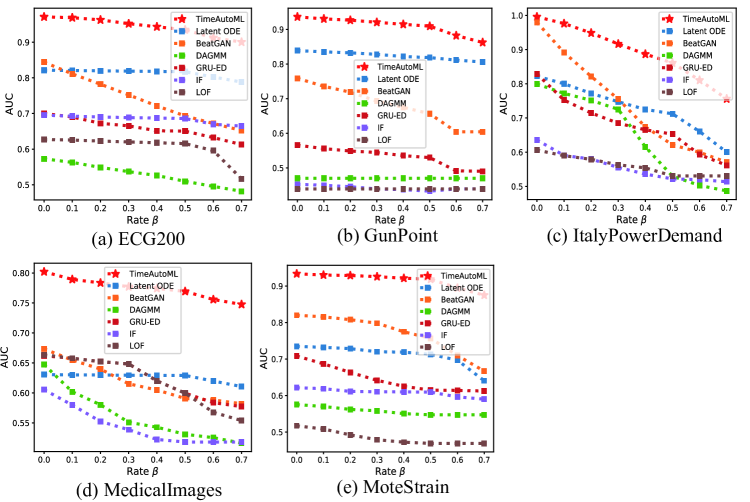
Figure A1: AUC scores of TimeAutoML and state-of-the-art anomaly detection methods on univariate datasets when irregular sampling rate $\beta$ varies from 0 to 0.7.

We investigate how the proposed TimeAutoML responds to contaminated training data when time series are irregularly sampled with the rate $\beta=0.5$. AUC scores of the proposed TimeAutoML when training on contaminated data are presented in Appendix D, Table A4, A5. We observe that the anomaly detection performance of TimeAutoML slightly degrades when training data are contaminated. Next, we investigate how TimeAutoML responds to different irregular sampling rate, i.e., when $\beta$ varies from 0 to 0.7. The AUC scores of TimeAutoML and state-of-the-art anomaly detection methods on ECGFiveDays dataset are presented in Fig 3 and the results on other datasets are presented in Appendix D, Fig A1, A2. We notice that TimeAutoML performs well robustly across multiple irregular sampling rates.

4.2 Visualization

In this section, we use a synthetic dataset to elucidate the underlying mechanism of TimeAutoML model for detecting time series anomalies. Figure 3 shows the latent space representation learned via TimeAutoML model from a synthetic dataset. In this dataset, smooth Sine curves are normal time series. The anomaly time series is created by adding noise to the normal time series over a short interval. It is evident from Figure 3 that the latent space representations of normal time series lie in a high density area that can be well characterized by a GMM; while the abnormal time series appears to deviate from the majority of the observations in the latent space. In short, the proposed encoder-decoder structure allows us to project the time series data in the original space onto vector representations in the latent space. In doing so, we can detect anomalies via clustering-based methods, e.g., GMM, and easily visualize as well as interpret the detected time series anomalies.

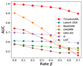
Figure 2: AUC scores of TimeAutoML on ECGFiveDays dataset when irregular sampling rate $\beta$ varies from 0 to 0.7.

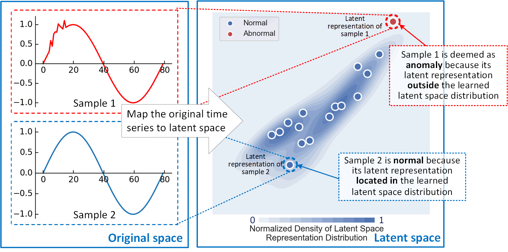
Figure 3: Anomaly interpretation via analysis in latent space.

4.3 Clustering

Apart from anomaly detection, TimeAutoML can be tailored for other machine learning tasks as well, e.g., multi-class clustering. In particular, the clustering process is carried out in the latent space via the GMM model, along with other modules in the pipeline.

We evaluate the effectiveness of TimeAutoML on three univariate time series datasets as well as two multivariate time series datasets. The NMI of TimeAutoML and state-of-the-art clustering methods are shown in Table 3. We observe that TimeAutoML generally achieves superior performance compared to baseline algorithms. This is because: i) it can automatically select the best module and hyperparameters; ii) the auxiliary classification task can enhance its representation capability.

Table 3: NMI scores of TimeAutoML and state-of-the-art clustering methods. Bold and underlined scores respectively represent the best and second-best performing methods.

Model	GunPoint		ECGFiveDays		ProximalPOAG		AtrialFibrillation		Epilepsy
	$\beta=0$	$\beta=0.5$	$\beta=0$	$\beta=0.5$	$\beta=0$	$\beta=0.5$	$\beta=0$	$\beta=0.5$	$\beta=0$	$\beta=0.5$
K-means	0.0011	0.0185	0.0002	0.0020	0.4842	0.0076	0	0	0.0760	0.1370
GMM	0.0063	0.0090	0.0030	0.0019	0.5298	0.0164	0	0	0.1276	0.0828
K-means+DTW	0.2100	0.0766	0.2508	0.0081	0.4830	0.4318	0.0650	0.1486	0.1454	0.1534
K-means+EDR	0.0656	0.0692	0.1614	0.0682	0.1105	0.0260	0.2025	0.1670	0.3064	0.2934
K-shape	0.0011	0.0280	0.7458	0.0855	0.4844	0.0237	0.3492	0.2841	0.2339	0.1732
SPIRAL	0.0020	0.0019	0.0218	0.0080	0.5457	0.0143	0.2249	0.1475	0.1600	0.1912
DEC	0.0263	0.0261	0.0148	0.1155	0.5504	0.1415	0.1242	0.1084	0.2206	0.1971
IDEC	0.0716	0.0640	0.0548	0.1061	0.5452	0.1122	0.1132	0.1242	0.2295	0.2372
DTC	0.3284	0.0714	0.0170	0.0162	0.4154	0.0263	0.1443	0.1331	0.2036	0.0886
DTCR	0.0564	0.0676	0.3299	0.1415	0.5190	0.3392	0.4081	0.3593	0.3827	0.2583
TimeAutoML	0.3262	0.2794	0.5914	0.3220	0.5915	0.5051	0.6623	0.6469	0.5073	0.4735
without $L_{\mathrm{self}}$
TimeAutoML	0.3323	0.2841	0.6108	0.3476	0.5981	0.5170	0.6871	0.6649	0.5419	0.5056

5 Conclusion

Representation learning on irregularly sampled time series is an under-explored topic. In this paper we propose a TimeAutoML framework to carry out unsupervised autonomous representation learning for irregularly sampled multivariate time series. In addition, we propose a self-supervised loss function to get labels directly from the unlabeled data. Strong empirical performance has been observed for TimeAutoML on a plurality of real-world datasets. While tremendous efforts have been undertaken for time series learning in general, AutoML for time series representation learning is still in its infancy and we hope the findings in this paper will open up new venues along this direction and spur further research efforts.

Appendix A Appendix A: Bayesian Optimization

Let $f(\theta)$ denote the objective function. Given function values during the preceding $T$ iterations $\bm{\underline{v}}=[f({\theta_{1}}),f({\theta_{2}}),\cdots,f({\theta_{T}})]$, we pick up the variable for sampling in the next iteration via solving the maxmization problem that involves the acquisition function i.e., expected improvement (EI) based on the postetior GP model.

Specifically, the objective function is assumed to follow a GP model (Shahriari et al., 2015) and can be expressed as $f(\theta)\sim GP(m(\theta),\bm{K})$, where $m(\theta)$ represents the mean function. And $\bm{K}$ represents the covariance matrix of $\{{\theta_{i}}\}_{i=0}^{T}$, namely, ${\bm{K}_{ij}}=\kappa({\theta_{i}},{\theta_{j}})$, where $\kappa(\cdot,\cdot)$ is the kernel function. In particular, the poster probability of $f(\theta)$ at iteration $T+1$ is assumed to follow a Gaussian distribution with mean $\mu(\theta^{\rm{*}})$ and covariance ${\sigma^{2}}(\theta^{\rm{*}})$, given the observation function values $\bm{\underline{v}}$ :

$$\begin{array}[]{l}\mu(\theta^{\rm{*}})={\bm{\underline{\kappa}}^{T}}{[\bm{K}+\sigma_{n}^{2}{\rm\bm{I}}]^{-1}}\bm{\underline{v}},\\ \sigma^{2}(\theta^{\rm{*}})=\kappa(\theta^{\rm{*}},\theta^{\rm{*}})-{\bm{\underline{\kappa}}^{T}}{[\bm{K}+\sigma_{n}^{2}{\rm\bm{I}}]^{-1}}\bm{\underline{\kappa}},\end{array}$$ (9)

where $\bm{\underline{\kappa}}$ is a vector of covariance terms between $\theta^{\rm{*}}$ and $\{{\theta_{i}}\}_{i=0}^{T}$, and $\sigma_{n}^{2}$ denotes the noise variance. We choose the kenel function as ARD Matérn 5/2 kernel (Shahriari et al., 2015) in this paper:

$$\kappa(\bm{\underline{p}},\bm{\underline{p}}^{\prime})=\tau_{0}^{2}\exp(-\sqrt{5}r)(1+\sqrt{5}r+\frac{5}{3}{r^{2}}),$$ (10)

where $\bm{\underline{p}}$ and $\bm{\underline{p}}^{\prime}$ are input vectors, ${r^{2}}={\sum\nolimits_{i=1}^{d}{({\bm{\underline{p}}_{i}}-\bm{\underline{p}}^{\prime}_{i})}^{2}}/\tau_{i}^{2}$ , and $\psi=\{\{{\tau_{i}}\}_{i=0}^{d},\sigma_{n}^{2}\}$ are the GP hyperparameters which are determined by minimizing the negative log marginal likelihood $\log(y|\psi)$ :

$$\mathop{\min}\limits_{\psi}\log\det(\bm{K}+\sigma_{n}^{2}{\rm\bm{I}})+{\bm{\underline{v}}^{T}}{(\bm{K}+\sigma_{n}^{2}{\rm\bm{I}})^{-1}}\bm{\underline{v}}.$$ (11)

Given the mean $\mu(\theta^{\rm{*}})$ and covariance ${\sigma^{2}}(\theta^{\rm{*}})$ in (9), $\theta_{T+1}$ can be obtained via solving the following optimization problem:

$$\begin{array}[]{l}\begin{aligned} {\theta_{T+1}}\!&=\!\mathop{\arg\max}\limits_{{\theta^{\rm{*}}}}\mathrm{EI}(\!\theta^{\rm{*}}\!)\\ &=\!\mathop{\arg\max}\limits_{{\theta^{\rm{*}}}}(\!\mu(\!\theta^{\rm{*}}\!)\!-\!{y^{+}}\!)\Phi(\!\frac{{\mu(\!\theta^{\rm{*}}\!)\!-\!{y^{+}}}}{{\sigma(\!\theta^{\rm{*}}\!)}}\!)\!+\!\sigma\phi(\!\frac{{\mu(\!\theta^{\rm{*}}\!)\!-\!{y^{+}}}}{{\sigma(\!\theta^{\rm{*}}\!)}}\!),\end{aligned}\end{array}$$ (12)

where ${y^{+}}\!=\!\max[f({\theta_{1}}),f({\theta_{2}}),\cdots,f({\theta_{T}})]$ represents the maximum observation value in the previous $T$ iterations. $\Phi$ is normal cumulative distribution function and $\phi$ is normal probability density function. Through maximizing the EI acquisition function, we seek to improve $f(\theta_{T+1})$ monotonically after each iteration.

Appendix B Appendix B: Detailed Version of TimeAutoML

Input: $L$: pre-defined threshold for maximum number of iterations. $B$: pre-defined threshold for maximum Bayesian optimization iterations. $\bm{\underline{\alpha}}_{0}$ and $\bm{\underline{\beta}}_{0}$: pre-defined Beta distribution priors. $f_{\mathrm{upp}}$ and $f_{\mathrm{low}}$: pre-defined upper bound and lower bound to objective function $f$.

Set: $\bm{\underline{\alpha}}_{i}(t)\in\mathbb{R}^{Q_{i}}$, $\bm{\underline{\beta}}_{i}(t)\in\mathbb{R}^{Q_{i}}$: the cumulative reward and punishment for $i^{th}$ module for the $t^{th}$ iteration, specifically, $\bm{\underline{\alpha}}_{i}(1)=\bm{\underline{\alpha}}_{0}$ and $\bm{\underline{\beta}}_{i}(1)=\bm{\underline{\beta}}_{0}$.

for $t=1,2,\cdots,L$ do

       for $i=1,2,\cdots,M$ do

            Sample ${\bm{\underline{w}}_{i}}\sim\mathrm{Beta}({\bm{\underline{\alpha}}_{i}}(t),{\bm{\underline{\beta}}_{i}}(t))$

       end for

      

      Obtain the TimeAutoML pipeline configuration by solving the following optimization problem: $\mathop{{\mathop{\rm maxmize}\nolimits}}\limits_{\rm K}\sum\limits_{i=1}^{M}{{{({\bm{\underline{k}}_{i}})}^{\top}}}{\bm{\underline{w}}_{i}}\quad\text{subject to}\ {\bm{\underline{k}}_{i}}\in{\{0,1\}^{{Q_{i}}}},{1^{\top}}{\bm{\underline{k}}_{i}}=1,\forall i\in[M],$

      for $b=1,2,\cdots,B$ do

            Hyperparameters optimization: Update hyperparameters according to Bayesian optimization framework given in Appendix A and the obtained objective function value is denoted as $f({\rm K}(t),\Theta_{b}(t))$, where ${\rm K}(t)$ denote the module options in $t^{th}$ iteration and $\Theta_{b}(t)$ denote the hyperparameters in $b^{th}$ Bayesian optimization iteration in $t^{th}$ iteration.

       end for

      

      Update Beta distribution of the options in the configured pipeline:

      1. Let $f(t)=\max\{{{f({\rm K}(t),\Theta_{b}(t))}},b=1,\cdots,B\}$ denote the performance of TimeAutoML model at the $t^{th}$ iteration.

       2. Compute the continuous reward $\mathop{r}\limits^{\sim}$:

       $\mathop{r}\limits^{\sim}=\max\{0,\frac{{f(t)-{f_{\mathrm{low}}}}}{{{f_{\mathrm{upp}}}-{f_{\mathrm{low}}}}}\}$

      

      3. Obtain the binary reward $r\sim\mathrm{Bernoulli}(\mathop{r}\limits^{\sim})$.
for $i=1,2,\cdots,M$ do

            

$$\begin{array}[]{l}{\bm{\underline{\alpha}}_{i}}(t+1)={\bm{\underline{\alpha}}_{i}}(t)+{\bm{\underline{k}}_{i}}\cdot r\leavevmode\\ {\bm{\underline{\beta}}_{i}}(t+1)={\bm{\underline{\beta}}_{i}}(t)+{\bm{\underline{k}}_{i}}\cdot(1-r)\end{array}$$

       end for

      

end for

Output: A TimeAutoML model with optimized hyperparameters.

Algorithm 2 Detailed Version of TimeAutoML

It is seen that TimeAutoML consists of two main stages, i.e., pipeline configuration and hyperparameter optimization. In every iteration of TimeAutoML, Thompson sampling is utilized to refine the pipeline configuration at first. After that, Bayesian optimization is invoked to optimize the hyperparameters of the model. Finally, the Beta distribution of the chosen options will be updated according to the performance of the configured pipeline.

In the experiment, the upper limit to number of entire TimeAutoML iterations, BO iterations are set as 40 and 25 respectively. The Beta distribution priors are set respectively as $\alpha_{0}=10$ and $\beta_{0}=10$.

Appendix C Appendix C: Search Space: Options and Hyperparameters

Table A1: Modules, options, and hyperparameters of TimeAutoML.

Module	Options	Hyperparameters
Data augmentation	Scaling	Continuous and discrete hyperparameters
	Shifting	Discrete hyperparameters
	Time-warping	Discrete hyperparameters
Encoder	RNN	Discrete hyperparameters
	LSTM	Discrete hyperparameters
	GRU	Discrete hyperparameters
Attention	No attention	None
	Self-attention	None
Decoder	RNN	Discrete hyperparameters
	LSTM	Discrete hyperparameters
	GRU	Discrete hyperparameters
EM Estimator	Gaussian Mixture Model	Discrete hyperparameters
Similarity Selection	Relative Euclidean distance	None
	Cosine similarity	None
	Both	None
Estimation Network	Multi-layer feed-forward neural network	Discrete hyperparameters
Auxiliary Classification Network	Multi-layer feed-forward neural network	Discrete hyperparameters

C.1 Data augmentation

• Scaling: increasing or decreasing the amplitude of the time series. There are two hyperparametes, the number of data augmentation samples ${N^{\mathrm{aug}}}\in[0,100]$ and the scaling size ${h^{\mathrm{amp}}}\in[0.5,1.8]$.

• Shifting: cyclically shifting the time series to the left or right. There are two hyperparametes, the number of data augmentation samples ${N^{\mathrm{aug}}}\in[0,100]$ and the shift size ${h^{\mathrm{shift}}}\in[-10,10]$.

• Time-warping: randomly “slowing down” some timestamps and “speeding up” some timestamps. For each timestamp to “speed up”, we delete the data value at that timestamp. For each timestamp to “slow down”, we insert a new data value just before that timestamp. There are two hyperparametes, the number of data augmentation samples ${N^{\mathrm{aug}}}\in[0,100]$ and the number of time-warping timestamps ${h^{\mathrm{tm}}}\in[T/10,T/4]$.

C.2 Encoder

For all encoders, i.e. RNN, LSTM, and GRU, there is only one hyperparameter, i.e., the size of the encoder hidden state. And we assume it is no larger than 32, i.e., ${h^{\mathrm{enc}}}\in[1,32]$.

C.3 Attention

Self-attention mechanism has been considered in this framework.

C.4 Decoder

For all decoders, i.e. RNN, LSTM, and GRU, there is only one hyperparameter, i.e., the size of decoder hidden state ${h^{\mathrm{dec}}}$. For univariate time series, we assume it is no larger than 32, i.e., ${h^{\mathrm{dec}}}\in[1,32]$. And we assume ${h^{\mathrm{dec}}}\in[n^{\mathrm{feat}},4*n^{\mathrm{feat}}]$ for multivariate time series, where $n^{\mathrm{feat}}$ represents the dimension of the multivariate time series.

C.5 EM Estimator

In this module, we provide a statistical model GMM to carry out latent space representation distribution estimation. There is one hyperparameter, the number of mixture-component of GMM. EM algorithm is used to estimate the key parameters of GMM.

C.6 Similarity selection

We offer three similarity functions for selection, including relative Euclidean distance, cosine similarity, or the concatenation of both.

C.7 Estimation Network

We utilize a multi-layer neural network as the estimation network in our pipeline. There are two hyperparameters to be optimized, i.e., the number of layers ${e^{\mathrm{layer}}}\in[1,5]$ and the number of nodes in each layer ${e_{i}^{\mathrm{node}}}\in[8,128]$, $\forall 1\leq i\leq{e^{\mathrm{layer}}}$.

C.8 Auxiliary Classification Network

We utilize a multi-layer neural network as the auxiliary classification network in our pipeline. There are two hyperparameters to be optimized, i.e., the number of layers ${c^{\mathrm{layer}}}\in[1,5]$ and the number of nodes in each layer ${c_{i}^{\mathrm{node}}}\in[8,128]$, $\forall 1\leq i\leq{c^{\mathrm{layer}}}$.

Appendix D Appendix D: Result

D.1 Anomaly Detection Performance for Univariate Time Series

Table A2: AUC scores of TimeAutoML and state-of-the-art anomaly detection methods on UCR time series dataset when time series are regularly sampled ($\beta=0$). Bold and underlined scores respectively represent the best and second-best performing methods.

dataset	TimeAutoML	Latent ODE	BeatGAN	DAGMM	GRU-ED	IF	LOF
Adiac	1	1	1	1	1	0.9375	0.4375
ArrowHead	0.9876	0.8592	0.7923	0.872	0.4008	0.7899	0.442
Beef	1	1	1	1	0.8333	1	0.4167
BeetleFly	1	1	1	1	1	0.35	0.4
BirdChicken	1	1	0.8	0.9	0.6	0.5	0.4
Car	1	1	0.6233	0.3346	1	0.2854	0.4231
CBF	1	0.6573	0.9909	0.7983	0.8606	0.6408	0.9399
ChlorineConcentration	0.6653	0.5672	0.5291	0.5724	0.5048	0.5449	0.5899
CinCECGTorso	0.8951	0.6761	0.9966	0.7908	0.4958	0.6749	0.9641
Coffee	1	1	1	1	0.9333	0.75	0.7167
Computers	0.8354	0.744	0.738	0.6563	0.7686	0.468	0.5714
CricketX	1	0.9744	0.8754	0.8123	0.7892	0.7405	0.6282
CricketY	1	0.954	0.9828	0.8997	0.931	0.8161	0.9827
CricketZ	1	0.9583	0.8285	0.6897	0.8333	0.6521	0.6249
DiatomSizeReduction	1	0.8571	1	1	0.9913	0.9783	0.9946
DistalPhalanxOutlineAgeGroup	0.9912	0.8333	0.8	0.8333	0.6879	0.7021	0.6858
DistalPhalanxOutlineCorrect	0.8626	0.8333	0.5342	0.6721	0.6193	0.6204	0.7693
DistalPhalanxTW	1	0.9143	1	1	1	0.9643	1
Earthquakes	0.8418	0.7421	0.6221	0.5529	0.8033	0.5671	0.5428
ECG5000	0.9981	0.5648	0.9923	0.8475	0.8998	0.9304	0.5436
ElectricDevices	0.8427	0.5626	0.8381	0.7172	0.7958	0.5518	0.5528
FaceAll	1	0.7674	0.9821	0.9841	0.9844	0.7639	0.7847
FaceFour	1	1	1	1	0.9286	0.9286	0.4286
FacesUCR	1	0.6368	0.9276	0.9065	0.8786	0.6782	0.8296
FiftyWords	1	0.8187	0.9895	0.9901	0.5643	0.9474	0.807
Fish	1	0.9394	0.8523	0.7273	0.5909	0.4772	0.6212
FordA	0.6229	0.6204	0.5496	0.5619	0.6306	0.4963	0.4708
FordB	0.6008	0.6212	0.5999	0.6021	0.5949	0.5949	0.4971
Ham	0.8961	0.8579	0.6556	0.7667	0.6358	0.6348	0.6296
HandOutlines	0.8808	0.8362	0.9031	0.8524	0.5679	0.7349	0.7413
Haptics	0.8817	0.8579	0.7266	0.6698	0.5826	0.6674	0.5167
Herring	1	0.9581	0.8333	0.6528	0.8026	0.7231	0.7105
InlineSkate	0.8556	0.8039	0.65	0.7147	0.5559	0.4223	0.6254
InsectWingbeatSound	0.91	0.6574	0.9605	0.9735	0.7549	0.7861	0.9333
LargeKitchenAppliances	0.8708	0.7703	0.5887	0.5824	0.7975	0.5025	0.5289
Lightning2	1	0.9242	0.6061	0.7574	0.5758	0.909	0.7197
Lightning7	1	1	1	1	1	1	0.4211
Mallat	0.9996	0.6639	0.9979	0.9701	0.5728	0.8377	0.8811
Meat	1	1	1	0.975	1	0.7001	0.7001
MiddlePhalanxOutlineAgeGroup	1	0.954	0.9673	0.8512	0.7931	0.7414	0.431
MiddlePhalanxOutlineCorrect	0.9242	0.7355	0.4401	0.7012	0.7013	0.4818	0.5725
MiddlePhalanxTW	1	0.9524	1	1	1	0.9762	1
NonInvasiveFetalECGThorax1	1	0.9167	1	1	1	0.9306	0.8611
NonInvasiveFetalECGThorax2	1	0.9028	0.9167	1	1	0.9722	1
OliveOil	1	1	0.9167	0.9167	0.9167	0.9583	1
OSULeaf	1	0.8864	0.8125	0.8892	0.8352	0.375	0.6823
PhalangesOutlinesCorrect	0.7423	0.7049	0.4321	0.5521	0.6625	0.5192	0.6629
Phoneme	0.9148	0.6823	0.7054	0.5826	0.7964	0.4904	0.5943
Plane	1	1	1	1	1	1	0.4
ProximalPhalanxOutlineAgeGroup	0.998	0.8024	0.975	0.9723	0.9614	0.82	0.775
ProximalPhalanxOutlineCorrect	0.9255	0.6482	0.5823	0.7221	0.9051	0.5348	0.7474
ProximalPhalanxTW	1	0.8664	0.9663	0.9623	0.9079	0.8889	0.9311
RefrigerationDevices	0.9323	0.7483	0.7264	0.5722	0.5434	0.4665	0.5714
ScreenType	0.8572	0.7453	0.7453	0.5472	0.7686	0.4921	0.5289
ShapeletSim	1	0.9	0.7421	0.5721	0.9728	0.5611	0.5481
ShapesAll	1	1	0.9	0.95	1	0.85	0.95
SmallKitchenAppliances	0.9586	0.7151	0.6541	0.7321	0.9621	0.6812	0.6563
SonyAIBORobotSurface1	0.9998	0.6886	0.9982	0.9834	0.9991	0.8129	0.9731
SonyAIBORobotSurface2	0.9907	0.6211	0.9241	0.8994	0.9236	0.5981	0.7152
StarLightCurves	0.9135	0.5548	0.8083	0.8924	0.8386	0.8161	0.5028
Strawberry	0.7805	0.6786	0.6789	0.5659	0.8184	0.4738	0.4433
SwedishLeaf	0.9913	0.9394	0.6963	0.5758	0.6566	0.6212	0.6212
Symbols	0.9987	0.7669	0.9881	0.9762	0.947	0.8025	0.9942
SyntheticControl	1	1	0.736	0.6524	1	0.3299	0.66
ToeSegmentation1	0.9437	0.7112	0.8819	0.6264	0.5726	0.5226	0.6708
ToeSegmentation2	0.9907	0.8225	0.9358	0.8243	0.6157	0.5612	0.7021
Trace	1	1	1	1	1	0.9211	0.4211
TwoLeadECG	0.9959	0.6485	0.8759	0.6941	0.8641	0.5967	0.8274
TwoPatterns	0.9996	0.5899	0.9936	0.7163	0.9297	0.5411	0.7371
UWaveGestureLibraryAll	0.9941	0.6487	0.9935	0.9898	0.8106	0.9342	0.7896
UWaveGestureLibraryX	0.7477	0.6136	0.6563	0.6796	0.6009	0.5626	0.4696
UWaveGestureLibraryY	0.9845	0.6256	0.9742	0.9626	0.9357	0.9159	0.6244
UWaveGestureLibraryZ	0.9957	0.6587	0.9897	0.9883	0.9662	0.9161	0.8671
Wafer	0.9903	0.4947	0.9315	0.9586	0.6763	0.9436	0.5599
Wine	1	0.9536	0.8704	0.9074	0.7531	0.4259	0.6689
WordSynonyms	0.9929	0.7862	0.9862	0.9621	0.8245	0.8226	0.8442
Worms	0.9968	0.8485	0.8978	0.7677	0.7126	0.5341	0.5896
WormsTwoClass	0.9583	0.9375	0.6307	0.6957	0.7591	0.4021	0.4432
Yoga	0.7538	0.5823	0.6883	0.6766	0.5884	0.5421	0.6267

Table A3: AUC socores of TimeAutoML and state-of-the-art anomaly detection methods on UCR time series dataset when time series are irregularly sampled ($\beta=0.5$). Bold and underlined scores respectively represent the best and second-best performing methods.

dataset	TimeAutoML	Latent ODE	BeatGAN	DAGMM	GRU-ED	IF	LOF
Adiac	1	1	0.25	0.9375	1	0.4375	0.4
ArrowHead	0.9816	0.8095	0.7633	0.8671	0.3478	0.7547	0.442
Beef	1	1	1	1	1	0.5	0.4167
BeetleFly	1	1	0.9	0.75	1	0.35	0.35
BirdChicken	1	1	1	0.9	0.6	0.4	0.4
Car	1	1	0.6154	0.3077	0.6538	0.2692	0.4231
CBF	0.9933	0.6362	0.8725	0.7819	0.7638	0.5281	0.8849
ChlorineConcentration	0.5954	0.5669	0.4916	0.572	0.493	0.5171	0.5121
CinCECGTorso	0.876	0.6679	0.9037	0.7855	0.4931	0.6584	0.7881
Coffee	1	1	1	1	0.9333	0.75	0.4333
Computers	0.9188	0.5723	0.6613	0.635	0.72	0.456	0.5714
CricketX	1	0.9743	0.6731	0.8077	0.7051	0.7372	0.6282
CricketY	0.9897	0.9081	0.9639	0.8966	0.6897	0.8161	0.7989
CricketZ	1	0.9166	0.8125	0.6875	0.8333	0.6458	0.4375
DiatomSizeReduction	0.9793	0.8467	0.8104	1	0.6772	0.4848	0.6065
DistalPhalanxOutlineAgeGroup	0.9516	0.8395	0.7821	0.8333	0.6835	0.678	0.6755
DistalPhalanxOutlineCorrect	0.764	0.6759	0.5167	0.4941	0.5367	0.4719	0.4766
DistalPhalanxTW	1	0.9	1	1	1	0.9107	0.6643
Earthquakes	0.8191	0.6608	0.6083	0.5214	0.5841	0.5380	0.5248
ECG5000	0.9765	0.5422	0.8817	0.6795	0.8537	0.7008	0.5142
ElectricDevices	0.7481	0.5621	0.5288	0.6974	0.6679	0.5363	0.5331
FaceAll	1	0.6545	0.8552	0.6671	0.6892	0.6944	0.6528
FaceFour	1	1	1	0.9643	0.6429	0.6429	0.4286
FacesUCR	0.9491	0.6474	0.6296	0.891	0.5507	0.6765	0.6276
FiftyWords	0.997	0.7456	0.9684	0.9895	0.4532	0.8728	0.7149
Fish	0.9697	0.9393	0.8409	0.7727	0.4545	0.5	0.6212
FordA	0.6157	0.6037	0.5127	0.5414	0.6005	0.4958	0.4684
FordB	0.5808	0.6164	0.5212	0.587	0.5489	0.5352	0.4971
Ham	0.8812	0.8519	0.4778	0.7556	0.5278	0.6296	0.6296
HandOutlines	0.8504	0.6442	0.7287	0.8409	0.5425	0.6142	0.6266
Haptics	0.9353	0.8415	0.5547	0.6641	0.5223	0.5882	0.5167
Herring	0.9642	0.9474	0.7895	0.6491	0.5855	0.7105	0.7105
InlineSkate	0.8928	0.7281	0.5618	0.5691	0.5477	0.4088	0.5026
InsectWingbeatSound	0.8669	0.6515	0.8364	0.9137	0.6444	0.7139	0.8111
LargeKitchenAppliances	0.8375	0.7686	0.5433	0.569	0.5785	0.4905	0.4865
Lightning2	1	0.9015	0.4141	0.7475	0.4545	0.909	0.4934
Lightning7	1	1	1	1	1	0.9474	0.4211
Mallat	0.9888	0.6546	0.8948	0.9687	0.5512	0.6375	0.881
Meat	1	1	0.675	0.975	0.95	0.7001	0.7001
MiddlePhalanxOutlineAgeGroup	1	0.9081	0.9655	0.8448	0.6552	0.5574	0.431
MiddlePhalanxOutlineCorrect	0.7573	0.7195	0.4352	0.6543	0.4344	0.4738	0.4752
MiddlePhalanxTW	1	0.875	1	1	0.9952	0.8048	0.5524
NonInvasiveFetalECGThorax1	1	0.9028	0.8889	1	1	0.9583	0.7222
NonInvasiveFetalECGThorax2	1	0.8333	0.8148	1	1	0.9028	0.7222
OliveOil	1	1	0.5883	0.9583	0.5	0.4583	0.4167
OSULeaf	0.9955	0.8318	0.7184	0.7557	0.8227	0.375	0.6659
PhalangesOutlinesCorrect	0.6819	0.6671	0.4203	0.5372	0.5576	0.4466	0.4864
Phoneme	0.8898	0.6676	0.6135	0.5631	0.7821	0.4864	0.5692
Plane	1	1	1	1	1	1	0.4
ProximalPhalanxOutlineAgeGroup	0.998	0.723	0.861	0.965	0.925	0.72	0.5
ProximalPhalanxOutlineCorrect	0.8299	0.6398	0.5625	0.7033	0.5716	0.4972	0.4997
ProximalPhalanxTW	1	0.8333	0.8948	0.9603	0.842	0.875	0.5833
RefrigerationDevices	0.8799	0.6738	0.7047	0.5597	0.5268	0.4625	0.4284
ScreenType	0.8446	0.6954	0.7153	0.6137	0.8012	0.492	0.5714
ShapeletSim	0.9278	0.6901	0.7358	0.5056	0.6531	0.4444	0.5056
ShapesAll	1	1	0.9	0.95	0.9	0.85	0.95
SmallKitchenAppliances	0.9538	0.6812	0.6223	0.7218	0.9117	0.6692	0.6563
SonyAIBORobotSurface1	0.99	0.6833	0.8132	0.8001	0.9605	0.5227	0.7402
SonyAIBORobotSurface2	0.8206	0.6144	0.6641	0.7948	0.6927	0.5556	0.6126
StarLightCurves	0.9118	0.5489	0.795	0.8874	0.8324	0.8186	0.5028
Strawberry	0.7427	0.6733	0.5986	0.546	0.5672	0.4643	0.4433
SwedishLeaf	0.9889	0.9318	0.6566	0.5758	0.4949	0.4949	0.4734
Symbols	0.9961	0.7437	0.982	0.9521	0.9303	0.7998	0.9636
SyntheticControl	1	0.968	0.704	0.62	0.5836	0.26	0.44
ToeSegmentation1	0.8917	0.7035	0.6944	0.5958	0.5632	0.5083	0.6708
ToeSegmentation2	0.9383	0.7624	0.8811	0.8113	0.4348	0.5485	0.6943
Trace	1	1	1	1	1	0.9211	0.4211
TwoLeadECG	0.8551	0.5865	0.6307	0.5512	0.6262	0.5429	0.5184
TwoPatterns	0.9981	0.5877	0.8861	0.6994	0.8026	0.5271	0.7253
UWaveGestureLibraryAll	0.9905	0.6449	0.9858	0.9894	0.8058	0.9218	0.7575
UWaveGestureLibraryX	0.7011	0.6078	0.6428	0.6708	0.5054	0.5572	0.4696
UWaveGestureLibraryY	0.9839	0.6152	0.9744	0.96	0.9275	0.908	0.6198
UWaveGestureLibraryZ	0.9944	0.6393	0.9839	0.984	0.9595	0.9121	0.8527
Wafer	0.9572	0.4322	0.8668	0.9415	0.5939	0.8235	0.531
Wine	1	0.9477	0.4963	0.5024	0.5804	0.6778	0.6296
WordSynonyms	0.9687	0.723	0.9592	0.9387	0.7936	0.8107	0.8357
Worms	0.9924	0.803	0.8889	0.6667	0.7045	0.3333	0.5795
WormsTwoClass	0.9455	0.8	0.6307	0.6875	0.7531	0.375	0.4432
Yoga	0.7161	0.5726	0.6431	0.5919	0.5621	0.5359	0.5679

D.2 Anomaly Detection Performance for Univariate Time Series (Contaminated Training Dataset)

Table A4: AUC scores of TimeAutoML when univariate time series training datasets are contaminated with 5% and 10% anomaly samples.

Ratio	ECG200	ECGFiveDays	GunPoint	ItalyPowerDemand	MedicalImages	MoteStrain
${\rm{0\%}}$	0.9349	0.9719	0.9093	0.8811	0.7693	0.9186
${\rm{5\%}}$	0.9305	0.9697	0.8994	0.8624	0.7598	0.9104
${\rm{10\%}}$	0.9271	0.9624	0.8902	0.8466	0.7455	0.9043
Decline	0.78%	0.95%	1.91%	3.45%	2.38%	1.43%

D.3 Anomaly Detection Performance for Multivariate Time Series (Contaminated Training Dataset)

Table A5: AUC scores of TimeAutoML when univariate time series training datasets are contaminated with 5% and 10% anomaly samples.

Ratio	FingerMovements	LSST	RacketSports	PhonemeSpectra	Heartbeat	EthanolConcentration
${\rm{0\%}}$	0.9643	0.7827	0.9826	0.8685	0.7703	0.8561
${\rm{5\%}}$	0.9554	0.7643	0.9796	0.8623	0.7604	0.8425
${\rm{10\%}}$	0.9388	0.7559	0.9724	0.8601	0.7527	0.8379
Decline	2.55%	2.68%	1.02%	0.84%	1.76%	1.82%

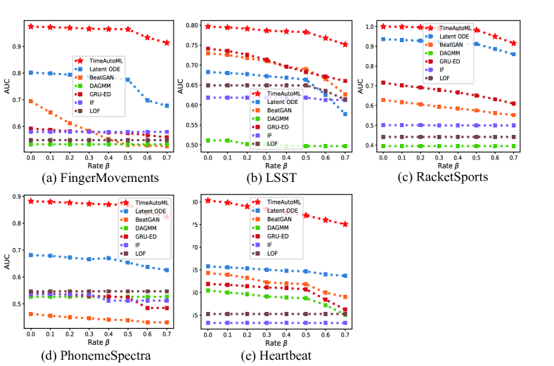
Figure A2: AUC scores of TimeAutoML and state-of-the-art anomaly detection methods on multivariate datasets when irregular sampling rate $\beta$ varies from 0 to 0.7.

Appendix E Illustration of irregular sampling

We provides an illustrative example to demonstrate how TimeAutoML remain robust against the irregularities in the sampling rates. Both regularly and irregularly sampled time series ($\beta=0.5$) are presented in Figure A3. And for the purpose of illustration we assume the normal time series is a Sine curve. The anomalous time series is obtained via adding noise to the normal time series over a short time interval. The irregularly sampling rate is set as 0.5 in this example.

As evident from the figure, the unusual pattern of the anomalous time series preserves after the irregular sampling. And such unusual pattern appears to be different from the distortion caused by irregular sampling. Due to the special characteristics of TimeAutoML, e.g., embedded LSTM encoder and attention mechanism, it is capable of learning both the short term and long term correlations among the training time series and therefore can detect such unusual pattern even in the presence of irregularity in the sampling.

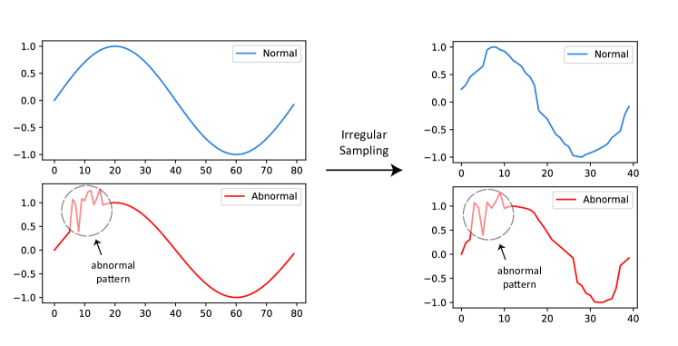
Figure A3: Irregular sampling on Sine curves.

References

- Abid & Zou (2018) Abubakar Abid and James Zou. Autowarp: Learning a warping distance from unlabeled time series using sequence autoencoders. In Proceedings of the 32nd International Conference on Neural Information Processing Systems, pp. 10568–10578, 2018.
- Bae et al. (2019) Woong Bae, Seungho Lee, Yeha Lee, Beomhee Park, Minki Chung, and Kyu-Hwan Jung. Resource optimized neural architecture search for 3D medical image segmentation. In International Conference on Medical Image Computing and Computer-Assisted Intervention, pp. 228–236. Springer, 2019.
- Bagnall et al. (2018) Anthony Bagnall, Hoang Anh Dau, Jason Lines, Michael Flynn, James Large, Aaron Bostrom, Paul Southam, and Eamonn Keogh. The uea multivariate time series classification archive, 2018. arXiv preprint arXiv:1811.00075, 2018.
- Bergstra & Bengio (2012) James Bergstra and Yoshua Bengio. Random search for hyper-parameter optimization. The Journal of Machine Learning Research, 13(1):281–305, 2012.
- Breunig et al. (2000) Markus M Breunig, Hans-Peter Kriegel, Raymond T Ng, and Jörg Sander. LOF: Identifying density-based local outliers. In Proceedings of the 2000 ACM SIGMOD international conference on Management of data, pp. 93–104, 2000.
- Cao et al. (2018) Wei Cao, Dong Wang, Jian Li, Hao Zhou, Lei Li, and Yitan Li. BRITS: Bidirectional recurrent imputation for time series. In Advances in Neural Information Processing Systems, pp. 6775–6785, 2018.
- Chan & Fu (1999) K. Chan and A. W. Fu. Efficient time series matching by wavelets. In ICDE, pp. 126–133, 1999.
- Chandola et al. (2008) Varun Chandola, Varun Mithal, and Vipin Kumar. Comparative evaluation of anomaly detection techniques for sequence data. In 2008 Eighth IEEE international conference on data mining, pp. 743–748. IEEE, 2008.
- Che et al. (2018) Zhengping Che, Sanjay Purushotham, Kyunghyun Cho, David Sontag, and Yan Liu. Recurrent neural networks for multivariate time series with missing values. Scientific reports, 8(1):1–12, 2018.
- Chen et al. (2018a) Junkun Chen, Kaiyu Chen, Xinchi Chen, Xipeng Qiu, and Xuanjing Huang. Exploring shared structures and hierarchies for multiple NLP tasks. arXiv preprint arXiv:1808.07658, 2018a.
- Chen et al. (2005) Lei Chen, M Tamer Özsu, and Vincent Oria. Robust and fast similarity search for moving object trajectories. In Proceedings of the 2005 ACM SIGMOD international conference on Management of data, pp. 491–502, 2005.
- Chen et al. (2018b) Ricky TQ Chen, Yulia Rubanova, Jesse Bettencourt, and David K Duvenaud. Neural ordinary differential equations. In Advances in neural information processing systems, pp. 6571–6583, 2018b.
- Chen et al. (2015) Yanping Chen, Eamonn Keogh, Bing Hu, Nurjahan Begum, Anthony Bagnall, Abdullah Mueen, and Gustavo Batista. The UCR time series classification archive, July 2015. www.cs.ucr.edu/~eamonn/time_series_data/.
- (14) Yukang Chen, Tong Yang, Xiangyu Zhang, Gaofeng Meng, Chunhong Pan, and Jian Sun. DETNAS: Neural architecture search on object detection.
- Faloutsos et al. (1994) C. Faloutsos, M. Ranganathan, and Y. Manolopoulos. Fast subsequence matching in time-series databases. In SIGMOD, pp. 419–429, 1994.
- Fan et al. (2020) Yang Fan, Fei Tian, Yingce Xia, Tao Qin, Xiang-Yang Li, and Tie-Yan Liu. Searching better architectures for neural machine translation. IEEE/ACM Transactions on Audio, Speech, and Language Processing, 2020.
- Fortuin et al. (2018) Vincent Fortuin, Matthias Hüser, Francesco Locatello, Heiko Strathmann, and Gunnar Rätsch. SOM-VAE: Interpretable discrete representation learning on time series. In International Conference on Learning Representations, 2018.
- Franceschi et al. (2019) Jean-Yves Franceschi, Aymeric Dieuleveut, and Martin Jaggi. Unsupervised scalable representation learning for multivariate time series. In Advances in Neural Information Processing Systems, pp. 4650–4661, 2019.
- Ghiasi et al. (2019) Golnaz Ghiasi, Tsung-Yi Lin, and Quoc V Le. NAS-FPN: Learning scalable feature pyramid architecture for object detection. In Proceedings of the IEEE conference on computer vision and pattern recognition, pp. 7036–7045, 2019.
- Guo et al. (2017) Xifeng Guo, Long Gao, Xinwang Liu, and Jianping Yin. Improved deep embedded clustering with local structure preservation. In IJCAI, pp. 1753–1759, 2017.
- Keogh et al. (2001) E. Keogh, Chakrabarti, M. K., Pazzani, and S. Mehrotra. Locally adaptive dimensionality reduction for indexing large time series databases. In SIGMOD, pp. 151–162, 2001.
- Kieu et al. (2019) Tung Kieu, Bin Yang, Chenjuan Guo, and Christian S Jensen. Outlier detection for time series with recurrent autoencoder ensembles. In IJCAI, pp. 2725–2732, 2019.
- Kim & Chi (2018) Yeo-Jin Kim and Min Chi. Temporal belief memory: Imputing missing data during rnn training. In In Proceedings of the 27th International Joint Conference on Artificial Intelligence (IJCAI-2018), 2018.
- Lei et al. (2019) Qi Lei, Jinfeng Yi, Roman Vaculin, Lingfei Wu, and Inderjit S Dhillon. Similarity preserving representation learning for time series clustering. In International Joint Conference on Artificial Intelligence, 2019.
- Liu et al. (2008) Fei Tony Liu, Kai Ming Ting, and Zhi-Hua Zhou. Isolation forest. In 2008 Eighth IEEE International Conference on Data Mining, pp. 413–422. IEEE, 2008.
- Luo et al. (2018) Yonghong Luo, Xiangrui Cai, Ying Zhang, Jun Xu, et al. Multivariate time series imputation with generative adversarial networks. In Advances in Neural Information Processing Systems, pp. 1596–1607, 2018.
- Luo et al. (2019) Yonghong Luo, Ying Zhang, Xiangrui Cai, and Xiaojie Yuan. E2GAN: End-to-end generative adversarial network for multivariate time series imputation. In Proceedings of the 28th International Joint Conference on Artificial Intelligence, pp. 3094–3100. AAAI Press, 2019.
- Ma et al. (2019) Qianli Ma, Jiawei Zheng, Sen Li, and Gary W Cottrell. Learning representations for time series clustering. In Advances in neural information processing systems, pp. 3781–3791, 2019.
- Madiraju et al. (2018) Naveen Sai Madiraju, Seid M Sadat, Dimitry Fisher, and Homa Karimabadi. Deep temporal clustering: Fully unsupervised learning of time-domain features. arXiv preprint arXiv:1802.01059, 2018.
- Malhotra et al. (2016) Pankaj Malhotra, Anusha Ramakrishnan, Gaurangi Anand, Lovekesh Vig, Puneet Agarwal, and Gautam Shroff. LSTM-based encoder-decoder for multi-sensor anomaly detection. arXiv preprint arXiv:1607.00148, 2016.
- Mathew et al. (2019) Anish Mathew, Sahely Bhadra, et al. Warping resilient time series embeddings. In Proceedings of the Time Series Workshop at ICML, 2019.
- Nekrasov et al. (2019) Vladimir Nekrasov, Hao Chen, Chunhua Shen, and Ian Reid. Fast neural architecture search of compact semantic segmentation models via auxiliary cells. In Proceedings of the IEEE Conference on computer vision and pattern recognition, pp. 9126–9135, 2019.
- Olsavszky et al. (2020) Victor Olsavszky, Mihnea Dosius, Cristian Vladescu, and Johannes Benecke. Time series analysis and forecasting with automated machine learning on a national ICD-10 database. International journal of environmental research and public health, 17(14):4979, 2020.
- Pang et al. (2019) Guansong Pang, Chunhua Shen, and Anton van den Hengel. Deep anomaly detection with deviation networks. In Proceedings of the 25th ACM SIGKDD International Conference on Knowledge Discovery & Data Mining, pp. 353–362, 2019.
- Paparrizos & Gravano (2015) John Paparrizos and Luis Gravano. K-shape: Efficient and accurate clustering of time series. In Proceedings of the 2015 ACM SIGMOD International Conference on Management of Data, pp. 1855–1870, 2015.
- Petitjean et al. (2011) François Petitjean, Alain Ketterlin, and Pierre Gançarski. A global averaging method for dynamic time warping, with applications to clustering. Pattern Recognition, 44(3):678–693, 2011.
- Rubanova et al. (2019) Yulia Rubanova, Ricky TQ Chen, and David K Duvenaud. Latent ordinary differential equations for irregularly-sampled time series. In Advances in Neural Information Processing Systems, pp. 5320–5330, 2019.
- Ruff et al. (2019) Lukas Ruff, Robert A Vandermeulen, Nico Görnitz, Alexander Binder, Emmanuel Müller, Klaus-Robert Müller, and Marius Kloft. Deep semi-supervised anomaly detection. arXiv preprint arXiv:1906.02694, 2019.
- Schölkopf et al. (2001) Bernhard Schölkopf, John C Platt, John Shawe-Taylor, Alex J Smola, and Robert C Williamson. Estimating the support of a high-dimensional distribution. Neural computation, 13(7):1443–1471, 2001.
- Shahriari et al. (2015) Bobak Shahriari, Kevin Swersky, Ziyu Wang, Ryan P Adams, and Nando De Freitas. Taking the human out of the loop: A review of bayesian optimization. Proceedings of the IEEE, 104(1):148–175, 2015.
- Shukla & Marlin (2019) Satya Narayan Shukla and Benjamin M Marlin. Interpolation-prediction networks for irregularly sampled time series. arXiv preprint arXiv:1909.07782, 2019.
- Syarif et al. (2016) Iwan Syarif, Adam Prugel-Bennett, and Gary Wills. SVM parameter optimization using grid search and genetic algorithm to improve classification performance. Telkomnika, 14(4):1502, 2016.
- (43) Arijit Ukil and Soma Bandyopadhyay. AutoSensing: Automated feature engineering and learning for classification task of time-series sensor signals.
- van Kuppevelt et al. (2020) D van Kuppevelt, C Meijer, F Huber, A van der Ploeg, S Georgievska, and VT van Hees. Mcfly: Automated deep learning on time series. SoftwareX, 12:100548, 2020.
- Weng et al. (2019) Yu Weng, Tianbao Zhou, Yujie Li, and Xiaoyu Qiu. NAS-UNET: Neural architecture search for medical image segmentation. IEEE Access, 7:44247–44257, 2019.
- Xie et al. (2016) Junyuan Xie, Ross Girshick, and Ali Farhadi. Unsupervised deep embedding for clustering analysis. In International conference on machine learning, pp. 478–487, 2016.
- Xu et al. (2019) Hang Xu, Lewei Yao, Wei Zhang, Xiaodan Liang, and Zhenguo Li. Auto-FPN: Automatic network architecture adaptation for object detection beyond classification. In Proceedings of the IEEE International Conference on Computer Vision, pp. 6649–6658, 2019.
- Yoon et al. (2019) Jinsung Yoon, Daniel Jarrett, and Mihaela van der Schaar. Time-series generative adversarial networks. In Advances in Neural Information Processing Systems, pp. 5508–5518, 2019.
- Zhou et al. (2019) Bin Zhou, Shenghua Liu, Bryan Hooi, Xueqi Cheng, and Jing Ye. BeatGAN: Anomalous rhythm detection using adversarially generated time series. In IJCAI, pp. 4433–4439, 2019.
- Zong et al. (2018) Bo Zong, Qi Song, Martin Renqiang Min, Wei Cheng, Cristian Lumezanu, Daeki Cho, and Haifeng Chen. Deep autoencoding gaussian mixture model for unsupervised anomaly detection. In International Conference on Learning Representations, 2018.