Piecewise-Linear Motion Planning
amidst Static, Moving, or Morphing Obstacles

Abstract

We propose a novel method for planning shortest length piecewise-linear motions through complex environments punctured with static, moving, or even morphing obstacles. Using a moment optimization approach, we formulate a hierarchy of semidefinite programs that yield increasingly refined lower bounds converging monotonically to the optimal path length. For computational tractability, our global moment optimization approach motivates an iterative motion planner that outperforms competing sampling-based and nonlinear optimization baselines. Our method natively handles continuous time constraints without any need for time discretization, and has the potential to scale better with dimensions compared to popular sampling-based methods.

I Introduction and Problem Statement

How should robots – viewed as complex systems of articulated rigid bodies – move from a start to a goal configuration in an environment cluttered with static and dynamic obstacles? Even without considering dynamic feasibility of a desired motion, mechanical and sensor limitations, uncertainty and feedback, the purely geometric motion planning problem is known to be computationally hard [26] in its full generality.

I-A The Optimal Motion Planning Problem

We follow a similar notation to that of [12] to describe the Optimal Motion Planning (OMP) problem. Let ${\mathcal{X}}={\mathbb{R}}^{n}$ be the configuration space, where $n\in{\mathbb{N}}$. We are interested in finding the shortest path ${\boldsymbol{x}}:[0,T]\rightarrow{\mathcal{X}}$ (where $T$ is a positive constant) that starts at a configuration ${\boldsymbol{x}}(0)={{\boldsymbol{x}}_{0}}\in{\mathcal{X}}$, ends at a configuration ${\boldsymbol{x}}(T)={{\boldsymbol{x}}_{T}}\in{\mathcal{X}}$, and avoids a time-varying obstacle region ${\mathcal{X}}_{{\text{obs}}}(t)\subseteq{\mathcal{X}}$ at all times $t\in[0,T]$. Here, we assume that the obstacle-free space ${\mathcal{X}}_{\text{free}}(t)\coloneqq{\mathcal{X}}\setminus{\mathcal{X}}_{{\text{obs}}}(t)$ is a closed basic semialgebraic set, i.e., that there exists a (multivariate, scalar-valued) polynomial function $g_{k}\in\mathbb{R}[t,{\boldsymbol{x}}]$ in variables $t$ and ${\boldsymbol{x}}$ such that

$${\mathcal{X}}_{\text{free}}(t)\coloneqq\{{\boldsymbol{x}}\in\mathbb{R}^{n}\;|\;g_{1}(t,{\boldsymbol{x}})\geq 0,\ldots,g_{k}(t,{\boldsymbol{x}})\geq 0\}.$$

Our choice for working with polynomial functions to describe obstacles stems from two reasons. On the one hand, polynomial functions can uniformly approximate any continuous function over compact sets, and hence are powerful enough for modeling purposes. See figure 1 for an illustration of an obstacle morphing into a complex shape over time, as described by a degree-$7$ polynomial, and see [5, 7, 8, 24] for more examples on the use of polynomial functions for the purposes of modeling 3D geometry. On the other hand, as we will see in section II, the discovery of recent connections between algebraic geometry and semidefinite programming has resulted in powerful tools that are designed specifically for tackling optimization problems which are described by polynomial data.

More formally, the OMP problem described by data

$${\mathcal{D}}=({{\boldsymbol{x}}_{0}},{{\boldsymbol{x}}_{T}},\{g_{1},\ldots,g_{m}\}),$$ (1)

where ${{\boldsymbol{x}}_{0}},{{\boldsymbol{x}}_{T}}\in{\mathbb{R}}^{n}$ and $g_{1},\ldots,g_{m}\in{\mathbb{R}}[t,{\boldsymbol{x}}]$ is the following minimization problem,

$$\boxed{\begin{split}&\min_{{\boldsymbol{x}}:[0,T]\rightarrow{\mathbb{R}}^{n}}\quad\int_{0}^{T}\|\dot{\boldsymbol{x}}(t)\|\;{\rm d}t\\ &\;\textrm{s.t.}\quad{\boldsymbol{x}}(0)={{\boldsymbol{x}}_{0}}\,,\>{\boldsymbol{x}}(T)={{\boldsymbol{x}}_{T}},\\ &\;\quad\quad g_{k}(t,{\boldsymbol{x}}(t))\geq 0\quad\forall t\in[0,T],\;\forall k\in[m],\end{split}} {\mathcal{D}}$$ OMP()

where $\|\cdot\|$ denotes the $\ell_{2}$ norm, and $[s]$ denotes the set $\{1,\ldots,s\}$. The objective term $\int_{0}^{T}\|\dot{\boldsymbol{x}}(t)\|\;{\rm d}t$ is the length of the path ${\boldsymbol{x}}(t)$. A path that satisfies the constraints of OMP(${\mathcal{D}}$) is said to be feasible. A path that is feasible and has minimum length is said to be optimal.

Figure 1: Example of an time-varying obstacle described by the polynomial inequality $g(t,{\boldsymbol{x}})<0$, with $g(t,{\boldsymbol{x}})\coloneqq(1-t)(x_{1}^{2}+x_{2}^{2}+x_{3}^{2}+1)+\frac{t}{320}(320x_{1}^{2}x_{3}^{3}+36x_{2}^{2}x_{3}^{3}-5(4x_{1}^{2}+9x_{2}^{2}+4x_{3}^{2}-4)^{3})$. The shape of the obstacle changes from a sphere to a heart as time $t$ goes from $0$ to $1$.

I-B Background on Motion Planning

We first set the stage for describing and motivating our approach in relation to the vast prior literature [18, 9, 20] on motion planning. Most obviously, OMP(${\mathcal{D}}$) can be transcribed into a nonlinear optimization problem by using a parametric representation of the path together with time-discretization to construct a finite-dimensional optimization problem [28, 11, 30]. Because of its non-convexity, the effectiveness of such an approach depends on having a good initial guess and in general no guarantees can be provided that the process will not return a sub-optimal stationary point. Closely related is the body of work on virtual potential fields [13] where a vector field is designed to pull the robot towards the goal and push it away from obstacles. Unless a restricted class of navigation functions [27] generates the gradient flow, these methods are also susceptible to local minima. By contrast, sampling-based motion planners [19, 12, 10], pervasively used in robotics, are attractive since they can at-least offer a guarantee of probabilistic completeness, that is, as the planning time goes to infinity, the probability of finding a solution tends to one. Sampling-based planners rely on a collision checking primitive to construct a data structure, e.g., tree or a graph, that stores a sampling of obstacle-avoiding feasible motions of the robot. In their most common instantiations, sampling methods return feasible paths, not necessarily optimal [12], almost alway also requiring post processing to reduce jerkiness.

Even in the time-independent, purely geometric path planning setting, the general problem of finding a feasible path, or correctly reporting that such a path does not exist, has been shown by Reif [26] to be PSPACE-hard. If ${\cal X}_{\text{free}}$ is semialgebraic, then its cylindrical cell decomposition [29] allows for a doubly-exponential (in the configuration space dimension $n$) solution to the motion planning problem. Canny’s Roadmap [6] gives an improved single-exponential solution based on the notion of a roadmap, a network of one-dimensional curves preserving the connectivity of the free space that can be reached from any configuration. However, despite their completeness guarantee, these techniques are considered computationally impractical for all but simple or low-degree-of-freedom problems.

It should be no surprise that dynamic environments where obstacles can appear, disappear, move or morph only magnify the hardness of general motion planning [25], even when the obstacle motion is pre-specifed as a function of time. Many planners can be adapted to this setting by simply defining the problem in a time-augmented state space. Then, the primary complication stems from the requirement that time must always increase along a path. An alternative is to decouple space and time planning by first finding a collision-free path in the absence of moving obstacles, and then determining a time scaling function. In any case, planners for time-varying problems may also become prone to failure simply due to discretization of time.

I-C Statement of Contributions

In this paper, we focus on solving the optimal motion planning problem for piecewise-linear motions. At the outset, it should be noted that even with this restriction, the problem remains PSPACE-hard [31]. With this setting, our contributions are as follows. First, we introduce a new arsenal of algorithmic and complexity-characterization tools from polynomial optimization and semidefinite programming (SDP) to the motion planning literature. Specifically, for any optimal motion problem OMP(${\mathcal{D}}$) described by data ${\mathcal{D}}$ as in (1), and for any number of pieces $s$, we present a hierarchy of semidefinite programs SDP$(r,s;{\mathcal{D}})$ indexed by a scalar $r$. Every level of this hierarchy provides a lower bound $\rho(r,s;{\mathcal{D}})$ on the minimum length $\rho(s;{\mathcal{D}})$ attained by piecewise-linear paths that are feasible to OMP(${\mathcal{D}}$) and have $s$ pieces. Importantly, we provide the asymptotic guarantee that $\rho(r,s;{\mathcal{D}})\rightarrow\rho(s;{\mathcal{D}})$ as $r\rightarrow\infty$. This notion of asymptotic completeness is analogous to probabilistic completeness in sampling-based methods, in the sense that in the limit of increasing computation, we are guaranteed to optimally solve the problem, or declare that no solution exists.

To remain computationally competitive with practical motion planners, we also derive a sequential SDP-based method called Moment Motion Planner (MMP). Unlike previously proposed planners for dynamic obstacle avoidance, MMP natively handles continuous-time constraints, does not require any discretization, and relies on semidefinite programs whose size scales polynomially in configuration space dimensionality. On several benchmark problems involving static, moving and morphing obstacles in dimension $2$, $3$, and $4$, including a bimanual planar manipulation task, MMP consistently outperforms RRT and nonlinear programming based baselines, while returning smoother paths in comparable solve time.

II Moment-based approach for time-varying optimization problems

The last few decades have known the emergence of a powerful moment-based approach for solving optimizaton problems that are described by polynomial data [17]. One of the main challenges one faces when applying this moment approach to the motion planning problem OMP(${\mathcal{D}}$) is the fact that solutions (and the constraints on these solutions) vary continuously with time. For clarity of presentation, we first ignore the complexities arising from this time dependence and present the basic ideas behind this approach. Then, we present a result from real algebraic geometry on sum of squares representations of univariate polynomial matrices that will allow us to impose time-varying constraints on time-varying solutions.

Let us recall some standard notation. For any vector ${\boldsymbol{\alpha}}\in{\mathbb{N}}^{n}$, $|{\boldsymbol{\alpha}}|$ denotes $\sum_{i=1}^{n}\alpha_{i}$. We denote by ${\mathbb{N}}^{n}_{d}$ the set of vectors ${\boldsymbol{\alpha}}\in{\mathbb{N}}^{n}$ that satisfy $|{\boldsymbol{\alpha}}|\leq d$. We denote by ${\mathbb{R}}[{\boldsymbol{y}}]$ the set of (scalar valued) polynomial functions in the variables $y_{1},\ldots,y_{n}$. For ${\boldsymbol{\alpha}}\in{\mathbb{N}}^{n}$, the monomial $y_{1}^{\alpha_{1}}\ldots y_{n}^{\alpha_{n}}$ is denote by ${\boldsymbol{y}}^{\boldsymbol{\alpha}}$, and the coefficient of a polynomial $p\in{\mathbb{R}}[{\boldsymbol{y}}]$ corresponding to the monomial ${\boldsymbol{y}}^{\boldsymbol{\alpha}}$ is denoted by $p_{\boldsymbol{\alpha}}$. The degree of the monomial ${\boldsymbol{y}}^{\boldsymbol{\alpha}}$ is $|{\boldsymbol{\alpha}}|$, and the degree $\deg p$ of a polynomial $p\in\mathbb{R}[{\boldsymbol{y}}]$ is the maximum degree of its monomials. We denote by ${\mathbb{R}}_{d}[{\boldsymbol{y}}]$ the set of polynomials of degree smaller than or equal to $d$.

II-A Moment Approach for Polynomial Optimization Problems

A polynomial optimization problem is a problem of the form

$$\begin{split}p^{*}\,=\,\min_{{\boldsymbol{y}}\in\mathbb{R}^{n}}\quad&p({\boldsymbol{y}})\\ \text{s.t.}\quad&h_{k}({\boldsymbol{y}})=0\quad k\in[m_{1}],\\ \text{s.t.}\quad&g_{k}({\boldsymbol{y}})\geq 0\quad k\in[m_{2}],\end{split}$$ (P)

where $p,h_{1},\ldots,h_{m_{1}},g_{1},\ldots,g_{m_{2}}\in{\mathbb{R}}[{\boldsymbol{y}}]$. In general, problem equation P is nonconvex and is very challenging to solve. In fact it is NP-hard even when $m_{1}=0$, $m_{2}=0$, and $p$ is a polynomial of degree four (see, e.g., [21]). An approach pioneered in [14] has been to replace the feasible set

$$K\coloneqq\{{\boldsymbol{y}}\in{\mathbb{R}}^{n}\;|\;h_{k}({\boldsymbol{y}})=0\;\forall k\in[m_{1}],\;g_{k}({\boldsymbol{y}})\geq 0\;\forall k\in[m_{2}]\}$$

with the set ${\mathcal{M}}(K)_{+}$ of nonnegative Borel measures on $K$ of total mass equal to one, leading to the optimization problem

$$\min_{\mu\in{\mathcal{M}}(K)_{+}}\quad\int p({\boldsymbol{y}})\;{\rm d}\mu.$$ (2)

It is not hard to see that the optimal value of problem equation 2 is equal to that of equation P. Moreover, problem equation 2 has a linear objective function and a convex (infinite-dimensional) feasible set.

We will now explain how to obtain a finite dimensional, convex relaxation of equation 2. The key idea is to view equation 2 not as an optimization problem over measures $\mu\in{\mathcal{M}}(K)_{+}$, but as an optimization problem over sequences of moments $\{\int{\boldsymbol{y}}^{{\boldsymbol{\alpha}}}d{\mu}\}_{{\boldsymbol{\alpha}}\in{\mathbb{N}}^{n}}$ of measures $\mu\in{\mathcal{M}}(K)_{+}$. This is possible because the objective function $\int p({\boldsymbol{y}}){\rm d}\mu=\sum_{|{\boldsymbol{\alpha}}|\leq\deg p}{\boldsymbol{p}}_{{\boldsymbol{\alpha}}}\int{\boldsymbol{y}}^{{\boldsymbol{\alpha}}}d{\mu}$ of problem equation 2 only depend on the measure $\mu$ through its first few moments.

Before we move further with the explanation of the moment approach, we need to introduce some additional notation. For any integer $r\in{\mathbb{N}}$, we denote by ${\mathcal{M}}_{r,n}$ the set of truncated sequences of “pseudo-moments” in $n$ variables, i.e., elements of the form $(\phi_{\boldsymbol{\alpha}})_{{\boldsymbol{\alpha}}\in{\mathbb{N}}_{r}^{n}},$ where $\phi_{\boldsymbol{\alpha}}\in{\mathbb{R}}$ for every ${\boldsymbol{\alpha}}\in{\mathbb{N}}_{r}^{n}$. Note that any measure $\mu$ gives rise to an element of ${\mathcal{M}}_{r,n}$, namely, $\left(\int{\boldsymbol{y}}^{{\boldsymbol{\alpha}}}d{\mu}\right)_{{\boldsymbol{\alpha}}\in{\mathbb{N}}^{n}_{r}}\in{\mathcal{M}}_{r,n},$ but a general element of ${\mathcal{M}}_{r,n}$ might not come from a measure. For any $\phi\in{\mathcal{M}}_{r,n}$, we introduce the so-called Riesz functional $L_{\phi}:{\mathbb{R}}_{r}[{\boldsymbol{y}}]\rightarrow{\mathbb{R}}$ defined by

$$q\;\left(=\sum_{{\boldsymbol{\alpha}}\in{\mathbb{N}}^{n}_{r}}q_{\boldsymbol{\alpha}}x^{\boldsymbol{\alpha}}\right)\mapsto\sum_{{\boldsymbol{\alpha}}\in{\mathbb{N}}^{n}_{r}}\phi_{\boldsymbol{\alpha}}q_{\boldsymbol{\alpha}}.$$

The functional $L_{\phi}$ is to “pseudo-moments” what the expectation operator is to genuine moments. For $\phi\in{\mathcal{M}}_{r,n}$ and $q\in{\mathbb{R}}_{r}[{\boldsymbol{y}}]$, we denote by $M_{\phi}(q)$ the localization matrix associated with $q$ and $\phi$, i.e., the matrix

$$M_{\phi}(q)_{{\boldsymbol{\alpha}},{\boldsymbol{\beta}}}=L_{\phi}({\boldsymbol{y}}^{\boldsymbol{\alpha}}{\boldsymbol{y}}^{{\boldsymbol{\beta}}}q({\boldsymbol{y}}))\quad\forall{\boldsymbol{\alpha}},{\boldsymbol{\beta}}\in{\mathbb{N}}_{\lfloor(r-\deg q)/2\rfloor}^{n},$$

whose rows and columns are labeled by elements of ${\mathbb{N}}_{\lfloor(r-\deg q)/2\rfloor}^{n}$, where $\lfloor\cdot\rfloor$ is the floor function.

Now, for an integer $r$ larger than the maximum of the degrees of the polynomials $p,h_{1},\ldots,h_{m_{1}},g_{1},\ldots,g_{m_{1}}$, consider the moment relaxation of order $r$ of problem equation 2 given by

$$\min_{\phi\in{\mathcal{M}}_{r,n}} L_{\phi}(p)$$ (3)

s.t. $$L_{\phi}(1)\,=\,1\,;\>M_{\phi}(1)\succeq 0$$

$$L_{\phi}({\boldsymbol{y}}^{\alpha}h_{k})=0\;\forall{\boldsymbol{\alpha}}\in{\mathbb{N}}^{n}_{r-d_{k}},\;\forall k\in[m_{1}],$$

$$M_{\phi}(g_{k})\succeq 0,\;\forall k\in[m_{2}].$$

To see that problem (3) is indeed a relaxation of problem (2), take an arbitrary candidate measure $\mu\in{\mathcal{M}}(K)_{+}$ with corresponding objective value $v\coloneqq\int p({\boldsymbol{y}}){\rm d}\mu$ for problem (2), and let us extract from it the truncated sequence of moments $\phi\coloneqq(\int{\boldsymbol{y}}^{\boldsymbol{\alpha}}{\rm d}\mu)_{|{\boldsymbol{\alpha}}|\leq r}\in{\mathcal{M}}_{r,n}$ and show that $\phi$ is (i) feasible to problem (3) and (ii) has $v$ as objective value. To show (i), note that $L_{\phi}(1)=\int{\rm d}\mu=1$, and that the matrix $M_{\phi}(1)$ is positive semidefinite because for all polynomials $q\in{\mathbb{R}}_{r}[{\boldsymbol{y}}]$, ${\boldsymbol{q}}^{T}M_{\phi}(1){\boldsymbol{q}}=\int q^{2}({\boldsymbol{y}})\;{\rm d}\mu\geq 0,$ where ${\boldsymbol{q}}$ is the vector of coefficients of the polynomial $q$. A similar reasoning shows that $\phi$ satisfies all of the remaining constraints of problem equation 3. To show (ii), simply observe that $L_{\phi}(p)=\int p({\boldsymbol{y}}){\rm d}\mu=v.$ The constraints $L_{\phi}(1)\,=\,1$ and $M_{\phi}(1)\succeq 0$ do not depend on the data of the problem at hand. We refer to them as moment consistency constraints.

In general, it is not always possible to extract an optimal solution ${\boldsymbol{y}}\in{\mathbb{R}}^{n}$ of (P) from a ”pseudo-moment” solution $\phi\in\mathcal{M}_{r,n}$ of (3). However, under some conditons that hold generically (see, e.g., [22, 23]), there exists an order $r$ for which the optimal value of (3) is equal to that of (P), and an optimal solution ${\boldsymbol{y}}$ of (P) can be recovered from $\phi$ by a linear algebra routine. For more details related to extraction of solutions from moment relaxations, the interested reader is referred to [17].

For any $r\in{\mathbb{N}}$, problem equation 3 is an SDP that can be readily solved by off-the-shelf solvers such that MOSEK [2]. We remind the reader that an SDP is the problem of optimizing a linear function subject to linear matrix inequalities. SDPs can be solved to arbitrary accuracy in polynomial time. See [32] for a survey of the theory and applications of this subject.

Remark 1 (Notation for vector-valued variables)

In the rest of the paper, we will often deal with variables that are vector valued. To lighten our notation, we use ${\mathbb{R}}[{\boldsymbol{y}}_{1},\ldots,{\boldsymbol{y}}_{s}]$ (resp. ${\mathcal{M}}_{r,n_{1}+\ldots+n_{s}}$) to denote the set of polynomials (resp. truncated sequences of pseudo-moments) in all of the entries of the vector-valued variables ${\boldsymbol{y}}_{1}\in{\mathbb{R}}^{n_{1}},\ldots,{\boldsymbol{y}}_{s}\in{\mathbb{R}}^{n_{s}}$. We also write $({\boldsymbol{y}}_{1},\ldots,{\boldsymbol{y}}_{s})^{({\boldsymbol{\alpha}}_{1},\ldots,{\boldsymbol{\alpha}}_{s})}$ to denote the monomial ${\boldsymbol{y}}_{1}^{{\boldsymbol{\alpha}}_{1}}\ldots{\boldsymbol{y}}_{s}^{{\boldsymbol{\alpha}}_{s}}$, where for each $i\in[s]$, ${\boldsymbol{\alpha}}_{i}$ is an integer vector of the same size as ${\boldsymbol{y}}_{i}$.

II-B Extension to the time-varying setting.

In this paper, we are interested in a variation of problem (P) where the inequality constraints are time-varying, i.e., a variation where inequalties are of the form

$$g(t,{\boldsymbol{y}})\geq 0\quad\forall t\in[0,T],$$

where $g\in{\mathbb{R}}[t,{\boldsymbol{y}}]$. Such a constraint can be viewed as a continuum of constraints $g_{t}({\boldsymbol{y}})\geq 0$ indexed by $t\in[0,T]$, where $g_{t}\coloneqq g(t,\cdot)\in{\mathbb{R}}[{\boldsymbol{y}}]$. If we denote the univariate polynomial matrix $t\mapsto M_{\phi}(g_{t})$ by $X(t)$, then the moment approach explained above leads to the constraint

$$X(t)\succeq 0\quad\forall t\in[0,T].$$ (4)

The observation that the coefficients of the polynomial matrix $X$ depend linearly on the elements of $\phi$ combined with proposition 1 allows us to rewrite constraint equation 4 as a (nonvarying) semidefinite programming constraint on $\phi$. This allows us to circumvent the need for time discretization.

In the statement of proposition below, $S^{m}$ (resp. ${\mathbb{R}}_{d}^{m\times m}[t]$) denotes the set of symmetric matrices of size $m$ whose entries are elements of ${\mathbb{R}}$ (resp. ${\mathbb{R}}_{d}[t]$) for any positive integers $m$ and $d$.

Proposition 1 ([4] Univariate matrix Positivstellensatz)

Let $m$ and $d$ be positive integers. There exist two (explicit) linear maps $\lambda_{1}:S^{\lfloor\frac{d}{2}+1\rfloor m}\rightarrow{\mathbb{R}}_{d}^{m\times m}[t]$ and $\lambda_{2}:S^{\lfloor\frac{d}{2}+1\rfloor m}\rightarrow{\mathbb{R}}_{d}^{m\times m}[t]$ such that for $X\in{\mathbb{R}}_{d}^{m\times m}[t]$, $X(t)\succeq 0\;\forall t\in[0,T]$ if and only if there exist positive semidefinite matrices $Q_{1}$ and $Q_{2}$ of appropriate sizes that satisfy the equation $X=\lambda_{1}(Q_{1})+\lambda_{2}(Q_{2}).$

III Exact Moment Optimization Over piecewise-linear Paths

III-A Search for Piecewise-Linear Paths

We propose to approximate the shortest path of OMP(${\mathcal{D}}$) by piecewise-linear paths with a fixed number of pieces. We choose to work with the family of piecewise linear functions for two reasons. First, they can uniformly approximate any path over the time interval $[0,T]$ as the number of pieces grows. Second, fixing a low number pieces often leads to simpler and smoother paths.

More concretely, we fix a regular subdivision $\{0,\frac{T}{s},\frac{2T}{s},\ldots,T\}$ of the time interval $[0,T]$ of size $s$, and we parametrize our candidate trajectory ${\boldsymbol{x}}(t)$ as follows:

$${\boldsymbol{x}}(t)={\boldsymbol{u}}_{i}+t{\boldsymbol{v}}_{i}\quad\forall t\in\left[\frac{(i-1)T}{s},\frac{iT}{s}\right),\;\forall i\in[s],$$ (5)

where ${\boldsymbol{u}}_{i}$, ${\boldsymbol{v}}_{i}\in\mathbb{R}^{n}$ for $i=1,\ldots,s$. We rewrite the objective function and constraints of OMP(${\mathcal{D}}$) in this setting directly in terms of ${\boldsymbol{u}}\coloneqq({\boldsymbol{u}}_{1},\ldots,{\boldsymbol{u}}_{s})$ and ${\boldsymbol{v}}\coloneqq({\boldsymbol{v}}_{1},\ldots,{\boldsymbol{v}}_{s})$. The objective function in OMP(${\mathcal{D}}$) can be expressed as $\frac{T}{s}\sum_{i=1}^{s}\|{\boldsymbol{v}}_{i}\|,$ and the obstacle-avoidance constraints become

$$g_{k}(t,{\boldsymbol{u}}_{i}+t{\boldsymbol{v}}_{i})\geq 0\quad\forall t\in\left[\frac{(i-1)T}{s},\frac{iT}{s}\right),\;\forall i\in[s],k\in[m].$$

To ensure continuity of the path ${\boldsymbol{x}}(t)$ at the grid point $i\frac{T}{s}$, for $i=0,\ldots,s$, we need to impose the additional constraint $h_{i}({\boldsymbol{u}},{\boldsymbol{v}})=0$ with

$$h_{i}({\boldsymbol{u}},{\boldsymbol{v}})\coloneqq{\boldsymbol{u}}_{i}+\frac{iT}{s}{\boldsymbol{v}}_{i}-\left({\boldsymbol{u}}_{i+1}+\frac{iT}{s}{\boldsymbol{v}}_{i+1}\right),$$

and the convention that ${\boldsymbol{u}}_{0}={{\boldsymbol{x}}_{0}}$, ${\boldsymbol{v}}_{0}=0$, ${\boldsymbol{u}}_{s+1}={{\boldsymbol{x}}_{T}}$, and ${\boldsymbol{v}}_{s+1}~{}=~{}0$.

In conclusion, when specialized to piecewise-linear paths of type equation 5, problem OMP(${\mathcal{D}}$) becomes

$$\boxed{\begin{aligned} &\rho(s;{\mathcal{D}})=\min_{{\boldsymbol{u}}_{i},{\boldsymbol{v}}_{i}\in}\quad\frac{T}{s}\sum_{i=1}^{n}\|{\boldsymbol{v}}_{i}\|\\ &\textrm{s.t.}\quad h_{i}({\boldsymbol{u}},{\boldsymbol{v}})=0\quad\forall i\in\{0,\ldots,{s+1}\}\\ &g_{k}(t,{\boldsymbol{u}}_{i}+t{\boldsymbol{v}}_{i})\geq 0\;\forall t\in\left[\frac{(i-1)T}{s},\frac{iT}{s}\right],\\ &\quad\quad\quad\quad\quad\quad\quad\quad\quad\quad\;k\in[m],\;i\in[s].\end{aligned}} \left(s;{\mathcal{D}}\right)$$ LMP

LMP$\left(s;{\mathcal{D}}\right)$ is a nonlinear, nonconvex optimization problem in the variables $({\boldsymbol{u}},{\boldsymbol{v}})$. The main difficulty comes from the global constraints

$$g_{k}(t,{\boldsymbol{u}}_{i}+t{\boldsymbol{v}}_{i})\geq 0\,,\quad\forall t\in\left[\frac{(i-1)T}{s},\frac{iT}{s}\right],\;\forall i\in~{}[s].$$ (6)

III-B A hierarchy of SDPs to find the best piecewise-linear path

For any optimal motion problem OMP(${\mathcal{D}}$), and for any number of pieces $s$, we present a hierarchy of semidefinite programs SDP$(r,s;{\mathcal{D}})$ indexed by a scalar $r$ with the following properties: (i) at every level $r$, the optimal value of SDP$(r,s;{\mathcal{D}})$ is a lower bound on that of LMP$\left(s;{\mathcal{D}}\right)$, (ii) under a compactness assumption, the the optimal value of SDP$(r,s;{\mathcal{D}})$ converges monotonically to that of LMP$\left(s;{\mathcal{D}}\right)$, and (iii) under a compactness and uniqueness assumption, the optimal solution of SDP$(r,s;{\mathcal{D}})$ converges to that of LMP$\left(s;{\mathcal{D}}\right)$.

As a preliminary step, for each piece $i\in[s]$, we introduce a scalar variable $z_{i}$ that represents the length $\|{\boldsymbol{v}}_{i}\|$ of that piece. Mathematically, we impose the constraints

$$h^{z}_{i}({\boldsymbol{u}},{\boldsymbol{v}},{\boldsymbol{z}})=0\text{ and }z_{i}\geq 0\quad i\in[s],$$ (7)

where $h^{z}_{i}({\boldsymbol{u}},{\boldsymbol{v}},{\boldsymbol{z}})=z_{i}^{2}-\left(\frac{T}{s}\|{\boldsymbol{v}}_{i}\|\right)^{2}$ for $i\in[s]$. We introduce the auxiliary variable $z_{i}$ in this seemingly complicated way (instead of simply taking $z_{i}=\|{\boldsymbol{v}}_{i}\|$) to make the functions appearing in the objective and constraints of LMP$\left(s;{\mathcal{D}}\right)$ polynomial functions.

We are now ready to follow the moment approach presented in section II. We fix a positive integer $r$, and we construct the moment relaxation of order $r$ of problem LMP$\left(s;{\mathcal{D}}\right)$. For that, we need to specify the decision variables, objective, and constraints. Our decision variable is a truncated sequence $\phi\in{\mathcal{M}}_{r}((2n+1)\times s)$ (that should be viewed as a sequence of “pseudo-moments” in variables ${\boldsymbol{u}}\in{\mathbb{R}}^{n\times s},{\boldsymbol{v}}\in{\mathbb{R}}^{n\times s}$, and ${\boldsymbol{z}}\in{\mathbb{R}}^{s}$ up to degree $r$). Intuitively, $\phi$ represents a “pseudo-distribution” over candidate paths. Our objective function is $\sum_{i=1}^{s}L_{\phi}(z_{i})$, and our constraints are the moment consistency constraints

$$L_{\phi}(1)=1\text{ and }M_{\phi}(1)\succeq 0,$$ (8)

the continuity constraints

$$L_{\phi}(({\boldsymbol{u}},{\boldsymbol{v}},{\boldsymbol{z}})^{\boldsymbol{\alpha}}h_{i}({\boldsymbol{u}},{\boldsymbol{v}}))=0$$ (9)

for all ${\boldsymbol{\alpha}}\in{\mathbb{N}}^{s(2n+1)}_{r-1}$ and $i\in\{0,\ldots,s\}$, the obstacle avoidance constraints

$$M_{\phi}(g_{k}(t,{\boldsymbol{u}}_{i}+t{\boldsymbol{v}}_{i}))\succeq 0\,\;\forall t\in\left[\frac{(i-1)T}{s},\frac{iT}{s}\right]$$ (10)

for all $k\in[m]$ and $i\in[s]$, and the constraints

$$L_{\phi}(({\boldsymbol{u}},{\boldsymbol{v}},{\boldsymbol{z}})^{\boldsymbol{\alpha}}h^{z}_{i}({\boldsymbol{u}},{\boldsymbol{v}},{\boldsymbol{z}}))=0\text{ and }M_{\phi}(z_{i})\succeq 0$$ (11)

coming from the definition of ${\boldsymbol{z}}$ in equation 7 for all ${\boldsymbol{\alpha}}\in{\mathbb{N}}^{s(2n+1)}_{r-2}$ and $i\in[s]$.

In conclusion, the moment relaxation of order $r$ of problem LMP$\left(s;{\mathcal{D}}\right)$ is the SDP

$$\small\boxed{\begin{aligned} \rho(r,s;{\mathcal{D}})=&\min_{\phi\in{\mathcal{M}}_{r,(2n+1)\times s}}\quad\sum_{i=1}^{s}L_{\phi}(z_{i})\\ &\textrm{s.t. $\phi$ satisfies \lx@cref{creftypepluralcap~refnum}{const:moment-consistency}, \lx@cref{refnum}{const:continuity}, \lx@cref{refnum}{const:z} and~\lx@cref{refnum}{const:obst-avoidance},}\end{aligned}} (r,s;{\mathcal{D}})$$ SDP

We emphasize that the objective function of SDP$(r,s;{\mathcal{D}})$ is linear, and that its constraints are valid SDP constraints. Indeed, constraints equations 8, 9 and 11 are (scalar or matrix) linear inequalities, while the time-varying inequalities in (10) translates to positive semidefinite constraints on the $\phi_{\boldsymbol{\alpha}}$’s and some additional auxiliary variables in view of Proposition 1.

Theorems 1 and 2 below present the main results of this section. They are related respectively to the optimal value and optimal solution of SDP$(r,s;{\mathcal{D}})$.

Theorem 1

Consider the motion planning problem OMP(${\mathcal{D}}$) given by data ${\mathcal{D}}=({{\boldsymbol{x}}_{0}},{{\boldsymbol{x}}_{T}},\{g_{1},\ldots,g_{m}\})$. The sequence $\{\rho(r,s)\}_{r\in{\mathbb{N}}}$ of optimal values of SDP$(r,s;{\mathcal{D}})$ is nondecreasing and is upper bounded by the optimal value $\rho(s;{\mathcal{D}})$ of LMP$\left(s;{\mathcal{D}}\right)$. (In particular, if $\rho(r,s;{\mathcal{D}})=\infty$ for some $r\in{\mathbb{N}}$, then problem LMP$\left(s;{\mathcal{D}}\right)$ is infeasible.) Furthermore, if

$$g_{m}(t,{\boldsymbol{x}})=R^{2}-\|{\boldsymbol{x}}\|^{2}\quad\forall{\boldsymbol{x}}\in{\mathbb{R}}^{n},\,\forall t\in{\mathbb{R}}\text{ for some $R>0$},$$ (12)

then $\rho(r,s;{\mathcal{D}})\rightarrow\rho(s;{\mathcal{D}})$ as $r\rightarrow\infty$.

Assumption (12) is needed for technical reasons but is not restrictive in practive. Indeed, in most motion planning problems, the configuration space is bounded, in which case we can append the polynomial $g(t,{\boldsymbol{x}})\coloneqq R^{2}-\|x\|^{2}$ to the list of polynomials in ${\mathcal{D}}$ without loss of generality.

Theorem 2

Consider the motion planning problem OMP(${\mathcal{D}}$) given by data ${\mathcal{D}}=({{\boldsymbol{x}}_{0}},{{\boldsymbol{x}}_{T}},\{g_{1},\ldots,g_{m}\})$. Under assumption (12), for any $r\in{\mathbb{N}}$, the optimal value of SDP$(r,s;{\mathcal{D}})$ is attained by some element $\phi^{r}\in{\mathcal{M}}_{r}({(2n+1)\times s})$. Furthermore, if LMP$\left(s;{\mathcal{D}}\right)$ has a unique optimal solution

$${\boldsymbol{x}}^{*}(t)\,:=\,{\boldsymbol{u}}_{i}^{*}+t\,{\boldsymbol{v}}_{i}^{*}\,,\>t\in\left[\frac{(i-1)T}{s},\frac{iT}{s}\right]\quad i\in[s],$$ (13)

then $L_{\phi^{r}}({\boldsymbol{u}}_{i})\rightarrow{\boldsymbol{u}}_{i}^{*}$ and $L_{\phi^{r}}({\boldsymbol{u}}_{i})\rightarrow{\boldsymbol{v}}_{i}^{*}$ as $r\rightarrow\infty$ for $i\in[s]$.

III-C Detecting optimality of a solution to SDP$(r,s;{\mathcal{D}})$

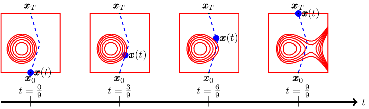
Figure 2: In red, setup of the path planning problem considered in example 1. In blue, the shortest piecewise-linear path extracted from SDP$(r,s;{\mathcal{D}})$ with $s=2$ and $r=6$.

The results of theorems 1 and 2 presented in the previous section are asymptotic. For a given number of pieces $s$ and a given relaxation order $r$, the optimal value of SDP$(r,s;{\mathcal{D}})$ provides only a lower bound on that of LMP$\left(s;{\mathcal{D}}\right)$. Recovering the shortest piecewise-linear path or its corresponding length requires taking $r$ to infinity in general. The following proposition shows that, if some conditons that are easily checkable hold, we can get the same recovery guarantees for finite $r$.

Proposition 2

For integers any integers $s$ and $n$, if an optimal solution $\phi\in{\mathcal{M}}_{r,(2n+1)\times s}$ of SDP$(r,s;{\mathcal{D}})$ satisfies $L_{\phi}(\|{\boldsymbol{u}}_{i}\|^{r})=\|L_{\phi}({\boldsymbol{u}}_{i})\|^{r},L_{\phi}(\|{\boldsymbol{v}}_{i}\|^{r})=\|L_{\phi}({\boldsymbol{v}}_{i})\|^{r}$, and $L_{\phi}(z_{i}^{r})=L_{\phi}(z_{i})^{r}$ for $i\in[s]$, then the piecewise-linear path

$${\boldsymbol{x}}^{*}(t)\,:=\,L_{\phi}({\boldsymbol{u}}_{i})+t\,L_{\phi}({\boldsymbol{v}}_{i})\quad\forall t\in\left[\frac{(i-1)T}{s},\frac{iT}{s}\right],\;\forall i\in[s],$$

is optimal for LMP$\left(s;{\mathcal{D}}\right)$.

Other than its obvious practical benefit, the result of proposition 2 inspires the iterative approach we present in section IV.

Example 1

Consider the simple instance of OMP(${\mathcal{D}}$) in dimension $n=2$ given by data ${\mathcal{D}}=({{\boldsymbol{x}}_{0}},{{\boldsymbol{x}}_{T}},\{g_{1}\ldots,g_{5}\})$, where ${{\boldsymbol{x}}_{0}}=(0,-1)^{T}$, ${{\boldsymbol{x}}_{T}}=(0,1)^{T}$, $g_{1}(t,{\boldsymbol{x}})=1-x_{1}$, $g_{3}(t,{\boldsymbol{x}})=1+x_{1},$ $g_{3}(t,{\boldsymbol{x}})=1-x_{2}$, $g_{4}(t,{\boldsymbol{x}})=1+x_{2},$ $g_{5}(t,{\boldsymbol{x}})=({\boldsymbol{x}}_{1}+\frac{1}{3})^{2}+({\boldsymbol{x}}_{2}-\frac{1}{5})^{2}-t({\boldsymbol{x}}_{1}+\frac{1}{3})^{3}-(\frac{1}{2})^{2}.$ (See figure 2 for a plot of this setup.) We search for paths that are piecewise-linear of the form in (5) with $s=2$ pieces. By computing the optimal values of SDP$(r,s;{\mathcal{D}})$ for $r\in\{3,4,5,6\}$, we obtain the nondecreasing sequence of lower bounds

$r$	3	4	5	6
SDP$(r,s;{\mathcal{D}})$	0.75	1.81	2.09	2.14

on the length of any piecewise-linear path with $2$ pieces that starts in ${{\boldsymbol{x}}_{0}}$, ends at ${{\boldsymbol{x}}_{T}}$, and avoids the obstacles given by the polynomials $\{g_{1},\ldots,g_{5}\}$. In particular, no such path has length smaller than $2.14$. We check numerically that for $r=6$, the optimal solution $\phi$ of SDP$(r,s;{\mathcal{D}})$ returned by the solver satisfies the requirement of proposition 2, and we extract from $\phi$ the path plotted in figure 2 whose length is $2.14$.

III-D A sparse version of the SDP hierarchy SDP$(r,s;{\mathcal{D}})$

In this section we briefly describe how one may reduce the size of the semidefinite programs SDP$(r,s;{\mathcal{D}})$ by exploiting an inherent sparsity of LMP$\left(s;{\mathcal{D}}\right)$. If we partition the decision variables $({\boldsymbol{u}},{\boldsymbol{v}},{\boldsymbol{z}})$ of LMP$\left(s;{\mathcal{D}}\right)$ as $V_{1}\cup\cdots\cup V_{s},$ where for each $i\in[s]$, $V_{i}\coloneqq\{{\boldsymbol{u}}_{i},{\boldsymbol{v}}_{i},z_{i},{\boldsymbol{u}}_{i+1},{\boldsymbol{v}}_{i+1},z_{i+1}\}$, then each constraint that appear in equation 9, equation 10, or equation 11 involves only the variables of exactly one of the $V_{i}$’s. Furthermore, the family $\{V_{1},\ldots,V_{s}\}$ satisfies the Running Intersection Property (RIP), that is,

$$\forall i\in[s-1],\;\exists k\leq i,\left(V_{1}\cup\ldots\cup V_{i}\right)\cap V_{i+1}\subset V_{k}.$$ (RIP)

Following [33, 15], we replace the single truncated sequence of “pseudo-moments” $\phi\in{\mathcal{M}}_{r,(2n+1)\times s}$ in all variables of $V$ with $s$ truncated sequences $\phi_{1},\ldots,\phi_{s}\in{\mathcal{M}}_{r,2n+1}$, where for each $i\in[s]$, $\phi_{i}$ is a truncated sequence of “pseudo-moments” in the variables of $V_{i}$. Intuitively, $\phi_{i}$ represents a “pseudo-distribution” from which the $i\text{-th}$ piece of our candidate piecewise-linear path is sampled. Without entering into details beyond the scope of this paper we can prove that theorems 1 and 2 hold if SDP$(r,s;{\mathcal{D}})$ is replaced with the SDP

$$\small\boxed{\begin{aligned} &\rho^{\prime}(r,s;{\mathcal{D}})=\min_{\phi_{i}}\quad\sum_{i=1}^{s}L_{\phi_{i}}(z_{i})\\ &\textrm{s.t.}\quad L_{\phi_{i}}(1)=1,\;M_{\phi_{i}}(1)\succeq 0,&i\in[s-1]\\ \ &L_{\phi_{i}}\left((V_{i},V_{i+1})^{\boldsymbol{\alpha}}\tilde{h}_{i}(V_{i},V_{i+1})\right)=0\,&\forall{\boldsymbol{\alpha}}\in{\mathbb{N}}^{4n}_{2r-1},\;i\in[s],\\ &L_{\phi_{i}}\left((V_{i},V_{i+1})^{\boldsymbol{\alpha}}\tilde{h}^{z}_{i}(V_{i})\right)=0\,&\forall{\boldsymbol{\alpha}}\in{\mathbb{N}}^{4n}_{2r-2},\;i\in[s],\\ &M_{\phi_{i}}(g_{k}(t,{\boldsymbol{u}}_{i}+t{\boldsymbol{v}}_{i}))\succeq 0&\forall t\in\left[\frac{(i-1)T}{s},\frac{iT}{s}\right],\\ &&k\in[m]\,;\,i\in[s-1],\end{aligned}} r,s;{\mathcal{D}}$$ SparseSDP()

where for each $i\in\{0,\ldots,s\}$, $\tilde{h}_{i}$ is the polynomial function such that $\tilde{h}_{i}(V_{i},V_{i+1})=h_{i}({\boldsymbol{u}},{\boldsymbol{v}})$, and for each $i\in[s]$, $\tilde{h}_{i}^{z}$ is the polynomial function such that $\tilde{h}^{z}_{i}(V_{i})=h^{z}_{i}({\boldsymbol{u}},{\boldsymbol{v}},{\boldsymbol{z}})$. The main feature of SparseSDP($r,s;{\mathcal{D}}$) when compared to SDP$(r,s;{\mathcal{D}})$ is that its constraints involve localizing matrices with pseudo-moments on $2(2n+1)$ variables (instead of $s(2n+1)$ variables in SDP$(r,s;{\mathcal{D}})$). For more details about the use of sparsity in polynomial optimization problems, interested reader is referred to [16].

Figure 3: Typical paths obtained for a motion planning problem in 2D. The path is constrained to be in the black box and should avoid the moving obstacles. Each obstacle is a sphere that moves with constant velocity (depicted by a red arrow).

$n$	Methods	Static Obstacles				Dynamic Obstacles
		success rate	length	smoothness	solve time	success rate	length	smoothness	solve time
$2$	RRT	40%	3.73	0.06	0.02	50%	3.59	0.12	0.06
	NLP	0%	nan	nan	nan	20%	3.4	0.06	0.06
	MMP	60%	3.0	0.03	0.43	50 %	2.85	0.03	0.43
$3$	RRT	50%	5.74	0.13	0.12	40%	4.82	0.1	0.23
	NLP	70%	3.44	0.05	0.12	60%	3.48	0.06	0.17
	MMP	100%	3.5	0.04	0.47	100%	3.55	0.04	0.47
$4$	RRT	60%	7.67	0.15	1.43	0%	nan	nan	nan
	NLP	80%	3.99	0.08	0.25	90%	4.34	0.1	0.2
	MMP	100%	4.11	0.05	0.55	100%	4.1	0.05	0.55

TABLE I: Average success, smoothness, and solve-time comparison of RRT, NLP and MMP (proposed) methods over 10 static and dynamic motion planning problems.

[noheader]trajImgs/double_pendulum/opttrajectoryall_small.csv

traj=Column4,=Column5,=Column6  traj=Column7,=Column8,=Column9 

traj=Column1,=Column2,=Column3 

Figure 4: Performance comparison of RRT, NLP, and MMP (proposed) methods on a bimanual planar manipulation task.

IV Moment Motion Planner: An Iterative Optimization Procedure Over piecewise-linear Paths

Algorithm 1 MMP: Moment Motion Planner

1:Input: Data ${\mathcal{D}}=(\{{{\boldsymbol{x}}_{0}},{{\boldsymbol{x}}_{T}},\{g_{1},\ldots,g_{m}\})$ order $r$ of the moment relaxation, number of iterations $N$, trade-off constant $\lambda>0$.

2:Initialize $\phi^{(0)}=(\phi^{(0)}_{1},\ldots,\phi^{(0)}_{s})$ randomly, where for each $i\in[s]$, $\phi^{(0)}_{i}\in{\mathcal{M}}_{r,2n}$.

3:for $t=1,\ldots,N$ do

4:     Let $\phi^{(t)}$ be a minimizer of (18) with $\bar{\phi}=\phi^{(t)}$ subject to equation 14, equation 15, and equation 16.

5:Return the piecewise-linear path defined by

$${\boldsymbol{x}}^{*}(t)\,:=\,L_{\phi_{i}^{(N)}}({\boldsymbol{u}}_{i})+t\,L_{\phi_{i}^{(N)}}({\boldsymbol{v}}_{i})$$

for every $t\in\left[\frac{(i-1)T}{s},\frac{iT}{s}\right]$ and every $i\in[s].$

As we have seen in the previous section, the optimal values $\rho(r,s)$ of the SDPs in the hieararchy SDP$(r,s;{\mathcal{D}})$ are nondecreasing lower bounds on the optimal value $\rho(s)$ of OMP(${\mathcal{D}}$). As a downside, a feasible path cannot possibly be extracted from a solution of one of these SDPs (at order, say, $r$) unless $r$ is large enough so that $\rho(r,s)=\rho(s)$. The order $r$ needed for that to happen is in general prohibitively large.

To adress this issue, we present in 4 a more practical motion planner called MMP. MMP is also based on a moment relaxation, but has two distinctive features when compared to SDP$(r,s;{\mathcal{D}})$: (i) it produces feasible paths already for low orders $r$ (taking $r=2$ produced good results in all of our benchmarks) and (ii) the optimal values produced by MMP are not necessarily lower bounds on $\rho(s)$. In other terms, MMP trades off some the theoretical guarantees of SDP$(r,s;{\mathcal{D}})$ for more efficiency.

MMP is an iterative algorithm. At every iteration, we solve an SDP that is similar in spirit to SDP$(r,s;{\mathcal{D}})$ with a few key differences. First, we drastically decrease the number of decision variables. We completely discard the variable ${\boldsymbol{z}}$, and we take inspiration from the sparsity considerations reviewed in section III-D to partition the remaining variables $({\boldsymbol{u}},{\boldsymbol{v}})$ of LMP$\left(s;{\mathcal{D}}\right)$ as $W_{1}\cup\cdots\cup W_{s},$ where for each $i\in[s]$, $W_{i}\coloneqq\{{\boldsymbol{u}}_{i},{\boldsymbol{v}}_{i}\}$. Then, we take as decision variables of our inner SDP $s$ truncated sequences $\phi\coloneqq(\phi_{1},\ldots,\phi_{s})$, where for each $i\in[s]$, $\phi_{i}\in{\mathcal{M}}_{r,2n}$ is a truncated sequence of “pseudo-moments” in variables $W_{i}$. Intuitively, each $\phi_{i}$ represents a “pseudo-distribution” from which the $i\text{-th}$ piece of our candidate piecewise-linear path is sampled. Note that the family of sets $\{W_{1},\ldots W_{s}\}$ does not satisfy the (RIP) property anymore. This is the main reason why MMP lacks some of the theoretical guarantees of the moment relaxation SDP$(r,s;{\mathcal{D}})$.

Then, we adapt the constraints of our inner SDP to our new choice of decision variables. In addition to the classical moment-consistency constraints

$$L_{{\phi_{i}}}(1)=1\text{ and }{\mathcal{M}}_{{\phi_{i}}}(1)\succeq 0\;\forall i\in[s],$$ (14)

we impose the the continuity constraints

$$L_{\phi_{i}}(({\boldsymbol{u}}_{i}+\frac{iT}{s}{\boldsymbol{v}}_{i})^{\boldsymbol{\alpha}})=L_{\phi_{i+1}}(({\boldsymbol{u}}_{i+1}+\frac{iT}{s}{\boldsymbol{v}}_{i+1})^{\boldsymbol{\alpha}})\;\forall{\boldsymbol{\alpha}}\in{\mathbb{N}}_{r-2}^{2n}$$ (15)

between endpoints of pieces $i$ and $i+1$ for each $i\in[s]$, and the obstacle-avoidance constraints

$$M_{\phi_{i}}(g_{k}(t,{\boldsymbol{u}}_{i}+t{\boldsymbol{v}}_{i}))\succeq 0\,\forall t\in\left[\frac{(i-1)T}{s},\frac{iT}{s}\right]$$ (16)

for each obstacle $k\in[m]$ and for each piece $i\in[s]$.

Finally, let us explain our choice of objective function. Motivated by proposition 2, we would ideally like to take the objective function of our SDP to be $\sum_{i=1}^{s}\|L_{{\phi_{i}}}({\boldsymbol{v}}_{i})\|+\lambda J(\phi),$ where $\lambda>0$ and

$$\begin{split}J(\phi)=&\sum_{i=1}^{s}L_{{\phi_{i}}}(\|{\boldsymbol{u}}_{i}\|^{r})-\|L_{{\phi_{i}}}({\boldsymbol{u}}_{i})\|^{r}\\ &+L_{{\phi_{i}}}(\|{\boldsymbol{v}}_{i}\|^{r})-\|L_{{\phi_{i}}}({\boldsymbol{v}}_{i})\|^{r}\end{split}$$ (17)

The intuition is that, if $J(\phi)=0$ for some $\phi=(\phi_{1},\ldots,\phi_{s})$ satisfying equations 15 and 16, then the path

$${\boldsymbol{x}}^{*}(t)\,:=\,L_{\phi_{i}}({\boldsymbol{u}}_{i})+t\,L_{\phi_{i}}({\boldsymbol{v}}_{i})\;\forall t\in\left[\frac{(i-1)T}{s},\frac{iT}{s}\right],\;\forall i\in[s],$$

is feasible to OMP(${\mathcal{D}}$). The constant $\lambda$ controls the trade-off between minimizing the length of the path and enforcing that the path is feasible. The issue with objective function (17) is that the function $J$ is nonconvex. As a workaroud, we replace $J$ in (17) with its linearization around a reference point $\bar{\phi}=(\bar{\phi}_{1},\ldots,\bar{\phi}_{s})$, leading to the objective function

$$\sum_{i=1}^{s}\|L_{{\phi_{i}}}({\boldsymbol{v}}_{i})\|+\lambda\bar{J}(\phi;\bar{\phi}),$$ (18)

where $\bar{J}(\phi;\bar{\phi})$ is given by

$$\begin{split}J(\bar{\phi})&+\sum_{i=1}^{s}L_{{\phi_{i}}}(\|{\boldsymbol{u}}_{i}\|^{r})-(r-1)L_{{\phi_{i}}}({\boldsymbol{u}}_{i})\|L_{{\bar{\phi}_{i}}}({\boldsymbol{u}}_{i})\|^{r-1}\\ &+L_{{\phi_{i}}}(\|{\boldsymbol{v}}_{i}\|^{r})-(r-1)L_{{\phi_{i}}}({\boldsymbol{v}}_{i})\|L_{{\bar{\phi}_{i}}}({\boldsymbol{v}}_{i})\|^{r-1}\end{split}$$

In the $t\text{-th}$ iteration of our iterative approach, we take the optimal solution $\phi^{{(t-1)}}$ obtained from solving the inner SDP at iteration $t-1$, and uses that as $\bar{\phi}$. The elements of $\phi^{(0)}$ are initialized from some random distribution. Gaussian initializaton seems to work well in practice. Note that the overall time complexity of 4 is polynomial in the dimension $n$, the number of iterations $N$, and the number of pieces $s$.

V Numerical Results

For animations of motion planning problems and code to reproduce numerical results, please see [1].

V-A MMP vs NLP vs RRT

Setup. In each dimension $n\in\{2,\ldots,4\}$, we generate $10$ motion planning problems where the path is constrained to live in the unit box $B=[-1,1]^{n}$ and must avoid $10$ static or dynamic spherical obstacles. More precisely, each motion planning problem is given by data ${\mathcal{D}}=({{\boldsymbol{x}}_{0}},{{\boldsymbol{x}}_{T}},\{g_{1},\ldots,g_{m}\})$, where ${{\boldsymbol{x}}_{0}}=(-1,\ldots,-1)\in{\mathbb{R}}^{n},{{\boldsymbol{x}}_{T}}=(1,\ldots,1)\in{\mathbb{R}}^{n}$, $i\in[n]$, $g_{i}({\boldsymbol{x}})=1-x_{i}$, $g_{i+n}(t,{\boldsymbol{x}})=1+x_{i}$ for $i\in[n]$, $g_{2n+k}(t,{\boldsymbol{x}})=\|{\boldsymbol{x}}-({\boldsymbol{c}}_{k}+t{\boldsymbol{v}}_{k})\|^{2}-\left(\frac{2}{10}\right)^{2}$. The centers ${\boldsymbol{c}}_{k}$ are sampled uniformly at random from $B$, the velocities ${\boldsymbol{v}}_{k}$ are either identically zero in the static case, or sampled uniformly from $B$ in the dynamic case. See figure 3 for an example of this setup in dimension $n=2$.

Comparison. In table I, we compare our MMP solver (with $r=2$, $N=20$, and $\lambda=0.1$) against a classical sampling-based technique (RRT) and basic nonlinear programming baseline (NLP) implemented with the help of the KNITRO.jl package [3]. MMP consistently achieves higher success rates, significantly shorter and smoother trajectories (the smoothness of a path ${\boldsymbol{x}}(t)$ is given by $\int_{0}^{T}\left(\dot{\boldsymbol{x}}(t)-\int_{0}^{T}\dot{\boldsymbol{x}}(s){\rm d}s\right)^{2}{\rm d}t$). The solve times are higher but remain highly practical.

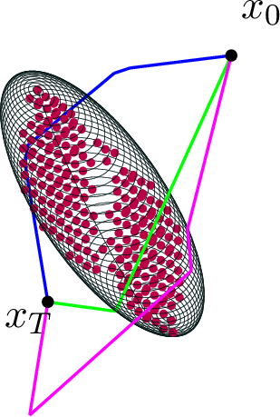
Figure 5: Plot of the paths found by RRT, NLP, and MMP (proposed) for the bimanual planning manipulation task of figure 4. The red dots depict values of the joint angles $(\alpha,\beta,\gamma)$ that would make the two arms collide. The black wireframe depicts the smallest enclosing ellipsoid containing the red dots.

V-B Bimanual Manipulation

As a proof of concept, we also consider a bimanual manipulation task requiring two two-link arms working collaboratively to go from an initial to goal configuration without colliding (see figure 4). For visualization, we restrict attention to planar manipulation problems involving planning in a configuration space of $3$ joint angles. First, we lift the obstacle set in cartesian space to joint angle space by evaluating all collision configurations on a grid over the $3$ joint angles. We then fit an enclosing ellipsoid (see figure 5) to obtain a semialgebraic description of the obstacle region in configuraton space. RRT finds a feasible path, but produces a jerky path involving an unnecessary recoiling of one of the arms. NLP fails to find a feasible path at all. MMP, with $3$ segments, succeeds in finding the shortest and smoothest path.

References

- [1] https://github.com/bachirelkhadir/PathPlanningSOS.jl.
- [2] Introducing the MOSEK optimization suite. 2018. URL https://docs.mosek.com/8.1/intro/index.html.
- [3] Knitro.jl. 2020. URL https://github.com/jump-dev/KNITRO.jl.
- [4] Amir Ali Ahmadi and Bachir El Khadir. Time-varying semidefinite programs. Preprint available at arXiv:1808.03994, 2018.
- [5] Amir Ali Ahmadi, Georgina Hall, Ameesh Makadia, and Vikas Sindhwani. Geometry of 3d environments and sum of squares polynomials. arXiv preprint arXiv:1611.07369, 2016.
- [6] John Canny. The complexity of robot motion planning. MIT press, 1988.
- [7] Fabrizio Dabbene and Didier Henrion. Set approximation via minimum-volume polynomial sublevel sets. In 2013 European Control Conference (ECC), pages 1114–1119. IEEE, 2013.
- [8] Fabrizio Dabbene, Didier Henrion, and Constantino M Lagoa. Simple approximations of semialgebraic sets and their applications to control. Automatica, 78:110–118, 2017.
- [9] Dan Halperin, Oren Salzman, and Micha Sharir. Algorithmic motion planning. In Handbook of Discrete and Computational Geometry, pages 1311–1342. Chapman and Hall/CRC, 2017.
- [10] Lucas Janson, Brian Ichter, and Marco Pavone. Deterministic sampling-based motion planning: Optimality, complexity, and performance. The International Journal of Robotics Research, 37(1):46–61, 2018.
- [11] Mrinal Kalakrishnan, Sachin Chitta, Evangelos Theodorou, Peter Pastor, and Stefan Schaal. Stomp: Stochastic trajectory optimization for motion planning. In 2011 IEEE international conference on robotics and automation, pages 4569–4574. IEEE, 2011.
- [12] Sertac Karaman and Emilio Frazzoli. Sampling-based algorithms for optimal motion planning. The international journal of robotics research, 30(7):846–894, 2011.
- [13] Oussama Khatib. Real-time obstacle avoidance for manipulators and mobile robots. In Autonomous robot vehicles, pages 396–404. Springer, 1986.
- [14] Jean B Lasserre. Global optimization with polynomials and the problem of moments. SIAM Journal on optimization, 11(3):796–817, 2001.
- [15] Jean B Lasserre. Convergent SDP-relaxations in polynomial optimization with sparsity. SIAM J. Optim., 17:822–843, 2006.
- [16] Jean B Lasserre. Moments, Positive Polynomials and Their Applications, volume 1. World Scientific, 2010.
- [17] Jean B Lasserre. An Introduction to Polynomial and Semi Algebraic Optimization. Cambridge University Press, 2015.
- [18] Steven M LaValle. Planning algorithms. 1999.
- [19] Steven M LaValle and James J Kuffner. Rapidly-exploring random trees: Progress and prospects. Algorithmic and computational robotics: new directions, (5):293–308, 2001.
- [20] Kevin M Lynch and Frank C Park. Modern Robotics. Cambridge University Press, 2017.
- [21] Katta G Murty and Santosh N Kabadi. Some NP-complete problems in quadratic and nonlinear programming. Mathematical Programming, 39:117–129, 1985.
- [22] J. Nie. Certifying convergence of Lasserre’s hierarchy via flat truncation. Mathematical Programming, Ser. A, 146(1-2):485–510, 2013.
- [23] J. Nie. Optimality conditions and finite convergence of Lasserre’s hierarchy. Mathematical Programming, Ser. A, 146(1-2):97–121, 2014.
- [24] Edouard Pauwels and Jean B Lasserre. Sorting out typicality with the inverse moment matrix sos polynomial. In Advances in Neural Information Processing Systems, pages 190–198, 2016.
- [25] John Reif and Micha Sharir. Motion planning in the presence of moving obstacles. Journal of the ACM (JACM), 41(4):764–790, 1994.
- [26] John H Reif. Complexity of the mover’s problem and generalizations. In 20th Annual Symposium on Foundations of Computer Science (sfcs 1979), pages 421–427. IEEE, 1979.
- [27] Elon Rimon and Daniel E Koditschek. Exact robot navigation using artificial potential functions. Departmental Papers (ESE), page 323, 1992.
- [28] John Schulman, Yan Duan, Jonathan Ho, Alex Lee, Ibrahim Awwal, Henry Bradlow, Jia Pan, Sachin Patil, Ken Goldberg, and Pieter Abbeel. Motion planning with sequential convex optimization and convex collision checking. The International Journal of Robotics Research, 33(9):1251–1270, 2014.
- [29] Jacob T Schwartz and Micha Sharir. On the piano movers’ problem: V. the case of a rod moving in three-dimensional space amidst polyhedral obstacles. Communications on Pure and Applied Mathematics, 37(6):815–848, 1984.
- [30] Vikas Sindhwani, Rebecca Roelofs, and Mrinal Kalakrishnan. Sequential operator splitting for constrained nonlinear optimal control. In 2017 American Control Conference (ACC), pages 4864–4871. IEEE, 2017.
- [31] Klaus Sutner and Wolfgang Maass. Motion planning among time dependent obstacles. Acta Informatica, 26(1-2):93–122, 1988.
- [32] Lieven Vandenberghe and Stephen Boyd. Semidefinite programming. SIAM review, 38(1):49–95, 1996.
- [33] H. Waki, S. Kim, M. Kojima, and M. Muramatsu. Sums of squares and semidefinite program relaxations for polynomial optimization problems with structured sparsity. SIAM J. Optim., 17(1):218–242, 2006.