Scaling Limits of Fluctuations of Extended-Source Internal DLA

David Darrow Supported in part by NSF Grant DMS 1500771.
Abstract

Abstract. In a previous work, we showed that the 2D, extended-source internal DLA (IDLA) of Levine and Peres is $\delta^{3/5}$-close to its scaling limit, if $\delta$ is the lattice size. In this paper, we investigate the scaling limits of the fluctuations themselves. Namely, we show that two naturally defined error functions, which measure the β€œlateness” of lattice points at one time and at all times, respectively, converge to geometry-dependent Gaussian random fields. We use these results to calculate point-correlation functions associated with the fluctuations of the flow. Along the way, we demonstrate similar $\delta^{3/5}$ bounds on the fluctuations of the related divisible sandpile model of Levine and Peres.

1 Introduction

Internal diffusion-limited aggregation (IDLA) is a lattice growth model, tracking the growth of a random set $A(t)\subset\mathbb{Z}^{d}$ defined as follows. At each time $t$, we start a particle at the origin, and we let it undergo a simple random until it first exits the set $A(t-1)$β€”supposing it exits at the point $z_{t}$, we set $A(t)=A(t-1)\cup\{z_{t}\}$. Intuitively, this process follows the diffusion of particles from an origin-centered source. In fact, it was originally proposed by the chemical physicists Meakin and Deutch [MD86] in order to model such diffusive processes, such as the smoothing of a spherical surface by electrochemical polishing.

We are interested in a generalization of this model to the extended-source case, wherein particles start instead from discretizations of a fixed mass distribution, and the lattice size is allowed to grow arbitrarily small. This generalization was first introduced and studied by Levine and Peres [LP08], although it corresponds to Diaconis and Fulton’s earlier notion of a β€œsmash sum” of two sets [DF91].

In both cases, a primary question of study is the overall smoothness of the occupied set $A(t)$. Following the work of Lawler, Bramson, and Griffeath [LBG92], it is well-known thatβ€”in the point-source caseβ€”these sets closely approximate an origin-centered ball for large $t$. Several authors have shown strong convergence rates for this process [Law95, AG10]; most recently, Jerison, Levine, and Sheffield proved that the fluctuations away from the disk are at most of order $\log t$ in dimension 2, narrowly improving a $\log^{2}t$ result by Asselah and GaudilliΓ¨re [JLS12, AG13a]. Independent works by Asselah and GaudilliΓ¨re and by Jerison, Levine, and Sheffield proved bounds of order $\sqrt{\log t}$ in higher dimensions [AG13b, JLS13], which have been shown to be tight [AG11]. In the extended-source case, Levine and Peres first showed that the scaling limits of IDLA correspond to solutions of a closely related free boundary problem [LP08]. We recently proved that, if the lattice size is $\delta$, the fluctuations of IDLA away from this expected set are at most of order $\delta^{3/5}$.

The fluctuations can also be studied β€œon the aggregate”, however, which provides interesting insight into the geometry of the problem. Namely, we are interested in studying mean fluctuations over an area of finite volume, as weighted by a test function $u\in C^{\infty}(\mathbb{R}^{d})$. To do this in the point-source case, Jerison et al [JLS14] introduced natural error functions on the lattice $\delta\mathbb{Z}^{d}$, which quantify how late or early the IDLA process is in getting to a given point. Specifically, they introduced a fluctuation function $E^{s}$ and a lateness function $L$, that capture fluctuations at a single time $s$ and at all times, respectively. They proved that these error functions weakly approach certain Gaussian random fields as the lattice spacing $\delta$ decreases, allowing them to find the scaling limits of fluctuations integrated against a test function $u$. Eli Sadovnik studied this question more recently for an extended source, in the special case of the single-time fluctuation function and with discrete harmonic test functions [Sad16].

In this paper, we extend the techniques used in [JLS14] and [Sad16] in order to prove more general scaling limits of random error functions in the extended-source case. Our main results, Theorems 3.1 and 3.2, show that the fluctuation function $E^{s}$ and the lateness function $L$ converge weakly to geometry-dependent Gaussian random fields, allowing for any $C^{4}$ test functions. In particular, by choosing highly localized test functions, we will be able to calculate β€œpoint-correlation functions”, which encode the correlations between fluctuations of IDLA at two different points in space.

It must be noted that, in the point-source case of [JLS14], the functions $E^{s}$ and $L$ measure fluctuations away from a previously-calculated continuous limit of IDLA; specifically, they measure the difference between $A(t)$ and a smooth sphere. To our knowledge, this is not possible in the general-source case without stronger estimates on the convergence of discrete harmonic functionsβ€”as such, our general-source versions of $E^{s}$ and $L$ compare IDLA to a closely related deterministic process: the discrete sandpile model of Levine and Peres [LP10]. We show in Theorem 2.7 that the discrete sandpile converges at least as quickly as the best known estimates (from [Dar20]) on IDLA. In fact, we believe that it converges faster than IDLA, but the estimate from Theorem 2.7 is sufficient for our purposes.

After briefly reviewing the necessary theory, we introduce our primary results in Section 3. The following sections are spent proving these results; Section 4 proves the scaling limit of the fixed-time fluctuation function, and Section 5 proves that of the lateness function. Finally, we use these results to calculate point correlation functions of IDLA fluctuations in Section 6.

2 Review of lattice growth processes

Here we provide a background on extended-source IDLA and on a related deterministic process, the divisible sandpile growth introduced also by Levine and Peres [LP08]. Many of our specific definitions are taken from our preceding paper, [Dar20]; see that paper for more information.

Following from [Dar20], we restrict attention to IDLA processes started from concentrated mass distributions.

Definition 2.1.

Let $D_{0}\subset\mathbb{R}^{2}$ be a compact, connected domain with smooth boundary, and fix $N\in\mathbb{Z}^{\geq 0}$ and $T_{1},...,T_{N}\in\mathbb{R}^{\geq 0}$. For each $i=1,...,N$ and $s\in[0,T_{i}]$, suppose $Q^{s}_{i}\subset D_{0}$ satisfies the following properties:

  1. 1.

    $Q_{i}^{s}$ is a compact domain with $\operatorname{Vol}(Q_{i}^{s})=s$.

  2. 2.

    $Q_{i}^{s}$ is bounded away from $\partial D_{0}$β€”that is, $Q_{i}^{s}\subset\subset\operatorname{int}(D_{0})$.

  3. 3.

    $Q_{i}^{s}\subset Q_{i}^{s^{\prime}}$ for $s\leq s^{\prime}\leq T_{i}$.

  4. 4.

    $\partial Q_{i}^{s}$ is rectifiable, with arclength bounded independently of $s$.

Finally, set $T=\sum_{k}T_{k}$, and fix increasing functions $s_{i}:[0,T]\to[0,T_{i}]$ satisfying βˆ‘ksk​(s)=ssubscriptπ‘˜subscriptπ‘ π‘˜π‘ π‘ \sum_{k}s_{k}(s)=s for all $s\in[0,T]$. In this setting, the concentrated mass distribution associated to the data $(D_{0},\{Q^{s}_{i}\},\{s_{i}\})$ is the map Οƒs:ℝ2β†’β„€β‰₯0:subscriptπœŽπ‘ β†’superscriptℝ2superscriptβ„€absent0\sigma_{s}:\mathbb{R}^{2}\to\mathbb{Z}^{\geq 0} defined by

Οƒs=𝟏D0+βˆ‘i=1N𝟏Qisi​(s).subscriptπœŽπ‘ subscript1subscript𝐷0superscriptsubscript𝑖1𝑁subscript1subscriptsuperscript𝑄subscript𝑠𝑖𝑠𝑖\sigma_{s}=\mathbf{1}_{D_{0}}+\sum_{i=1}^{N}\mathbf{1}_{Q^{s_{i}(s)}_{i}}.

In short, a concentrated mass distribution is a collection of increasing subsets $Q^{s_{i}}_{i}$ of $D_{0}$, such that the total mass at any time $s$ is $\operatorname{vol}(D_{0})+s$. The functions $s_{i}$ give the mass of each subset $Q^{s_{i}}_{i}$ at the time $s$.

The analysis of this paper holds in its entirety for infinite mass distributions, where $T=\infty$. For these, we simply require that the finite-time collections $\{Q_{i}^{s}\}|_{s\leq T^{\prime}}$ and {Οƒs}|s≀Tβ€²evaluated-atsubscriptπœŽπ‘ π‘ superscript𝑇′\{\sigma_{s}\}|_{s\leq T^{\prime}} give rise to concentrated mass distributions for any $T^{\prime}>0$. We will assume that $T<\infty$, but we can also imagine that we have simply β€œcut off” an infinite mass distribution in the manner just described.

Since we are studying processes on discrete lattices, we are primarily interested in the restrictions of these mass functions to the grid $\frac{1}{m}\mathbb{Z}^{2}$. Write Ssmsubscriptsuperscriptπ‘†π‘šπ‘ S^{m}_{s} for the multiset defined by βˆ‘1m​℀2(Οƒsβˆ’πŸD0)subscript1π‘šsuperscriptβ„€2subscriptπœŽπ‘ subscript1subscript𝐷0\sum\nolimits_{\frac{1}{m}\mathbb{Z}^{2}}(\sigma_{s}-\mathbf{1}_{D_{0}}); that is, for any $z\in\frac{1}{m}\mathbb{Z}^{2}\cap\bigcup Q_{i}^{s_{i}}$, we have that z∈Ssm𝑧subscriptsuperscriptπ‘†π‘šπ‘ z\in S^{m}_{s} with multiplicity Οƒs​(z)βˆ’1subscriptπœŽπ‘ π‘§1\sigma_{s}(z)-1. We can order $S^{m}_{T}$ into a sequence $z_{m,j}$ of source points as follows:

  1. 1.

    If $z\in S^{m}_{T}$ with multiplicity $k$, let $s_{i}(z):=\inf\{t\;|\;z\in S^{m}_{t}\;\text{with multiplicity}\;i+1\}$ for $i\leq k-1$.

  2. 2.

    Given $\{z_{m,1},...,z_{m,j-1}\}$, choose $z_{m,j}\in S^{m}_{T}\setminus\{z_{m,1},...,z_{m,j-1}\}$ to minimize $s_{i(z,j)}(z)$, where $i(z,j)$ is the multiplicity of $z$ in $\{z_{m,1},...,z_{m,j-1}\}$.

In short, we are simply ordering the particles in $S^{m}_{T}$ in the order they appear (accounting for multiplicity) in the sets {Ssm}subscriptsuperscriptπ‘†π‘šπ‘ \{S^{m}_{s}\}. Given this sequence, we define the discrete densities $\sigma_{m,n}=\mathbf{1}_{\frac{1}{m}\mathbb{Z}^{2}\cap D_{0}}+\sum_{i=1}^{n}\mathbf{1}_{\{z_{m,i}\}}$. It is clear that $\sigma_{m,n}$ differs from its continuum limit $\sigma_{n/m^{2}}$ at only $O(m^{-2})$ points, accounting for multiplicity.

The (resolution $m$) internal DLA (IDLA) associated with the mass distribution is the following process:

Definition 2.2 (Internal DLA).

Suppose we have a concentrated mass distribution with initial set $D_{0}$ giving rise to the sequences $\{z_{m,t}\}$. The IDLA $A_{m}(t)$ associated with the mass distribution is as follows. Define the initial set $A_{m}(0)=\frac{1}{m}\mathbb{Z}^{2}\cap D_{0}$. Then, for each integer $t\geq 1$, start a simple random walk at $z_{m,t}$, and let $z^{\prime}_{t}$ be the first point in the walk outside the set $A_{m}(t-1)$β€”then $A_{m}(t):=A_{m}(t-1)\cup\{z^{\prime}_{t}\}$.

Importantly, the law of $A_{m}(t)$ does not depend on the order of $\{z_{m,1},...,z_{m,t}\}$, as proven by Diaconis and Fulton [DF91, Lemma 2.2] (see [DF91, Section 3] for the application of this result to our setting).

For each time $s$, the sets $A_{m}(m^{2}s)$ approach a deterministic limit $D_{s}$ almost surely, where $D_{s}$ is the Diaconis–Fulton β€œsmash” sum

$$D_{s}=D_{0}\oplus Q_{1}^{s_{1}}\oplus\cdots\oplus Q_{N}^{s_{N}}.$$

The smash sum operation is as defined in [LP10]:

Definition 2.3.

If $A,B\subset\frac{1}{m}\mathbb{Z}^{2}$, we define the discrete smash sum $A\oplus B$ as follows. Let $C_{0}=A\cup B$, and for each $x_{i}\in\{x_{1},...,x_{n}\}=A\cap B$, start a simple random walk at $x_{i}$ and stop it upon exiting $C_{i-1}$. Let $y_{i}$ be its final position, and define $C_{i}=C_{i-1}\cup\{y_{i}\}$. Then $A\oplus B:=C_{n}$ is a random set.

As proven in [LP10, Theorem 1.3], if we instead take domains $A,B\subset\mathbb{R}^{2}$, the smash sums $A_{m}\oplus B_{m}$ of

$$A_{m}:=\frac{1}{m}\mathbb{Z}^{2}\cap A,\qquad B_{m}:=\frac{1}{m}\mathbb{Z}^{2}\cap B$$

approach a deterministic limit, which we label $A\oplus B$. Figure 1 (taken from [Dar20]) gives an example of this.

Refer to caption $A\cup B$ Refer to caption $A\oplus B$
Figure 1: The smash sum $A\oplus B$ is the deterministic limit of an IDLA-type growth process starting from the sets $A$ and $B$, representing the dispersal of particles in $A\cap B$ (in dark blue above) to the edges of $A\cup B$ (in yellow above).

The convergence $A_{m}(m^{2}s)\to D_{s}$ was shown originally by Levine and Peres [LP10]. In [Dar20, Theorem 3.1], we have recently shown the following convergence rate for this scaling limit, in the special case that $D_{s}$ is a smooth flowβ€”that is, that $s\mapsto D_{s}$ is a smooth isotopy for $s\in[0,T]$.

Lemma 2.4.

Suppose $D_{s}$ is a smooth flow arising from a concentrated mass distribution. For large enough $m$, the fluctuation of the associated IDLA $A_{m}(t)$ is bounded as

$$\mathbb{P}\bigg{\{}(D_{s})_{Cm^{-3/5}}\cap\frac{1}{m}\mathbb{Z}^{2}\subset A_{m}(m^{2}s)\subset(D_{s})^{Cm^{-3/5}}\;\text{for all}\;s\in[0,T]\bigg{\}}^{c}\leq e^{-m^{2/5}}$$

for a constant $C$ depending on the flow, where (Ds)Ξ΅superscriptsubscriptπ·π‘ πœ€(D_{s})^{\varepsilon} and (Ds)Ξ΅subscriptsubscriptπ·π‘ πœ€(D_{s})_{\varepsilon} denote outer- and inner-$\varepsilon$-neighborhoods of $D_{s}$, respectively.

In other words, the fluctuations of the random set $A_{m}(m^{2}s)$ are unlikely to be larger in magnitude than $Cm^{-3/5}$, for some fixed $C>0$. We will also use this to bound the maximum fluctuations of a closely related processβ€”the divisible sandpile growthβ€”defined as follows:

Definition 2.5 (Divisible Sandpile).

Suppose we have a concentrated mass distribution with initial set $D_{0}$ giving rise to the sequences $\{z_{m,i}\}$. The divisible sandpile aggregation associated with our mass distribution is characterized by its final mass distributions $\nu_{m,t}$. Let $\nu_{m,0}:=\mathbf{1}_{A_{m}(0)}=\mathbf{1}_{D_{0}\cap\frac{1}{m}\mathbb{Z}^{2}}$, and define $\nu_{m,n}$ inductively as follows.

Given $\nu_{m,n}$, define the intermediate function $\nu_{m,n}^{0}=\nu_{m,n}+\mathbf{1}_{\{z_{m,n+1}\}}$. At each time step $t$, choose a point $z=z(t)\in\operatorname{supp}\nu_{m,n}^{t}$ such that $\nu_{m,n}^{t}(z)>1$. Set

$$\nu_{m,n}^{t+1}(z)=1,\qquad\nu_{m,n}^{t+1}(z\pm 1/m)=\nu_{m,n}^{t}(z\pm 1/m)+\frac{1}{4}(\nu_{m,n}^{t}(z)-1),$$
$$\nu_{m,n}^{t+1}(z\pm i/m)=\nu_{m,n}^{t}(z\pm i/m)+\frac{1}{4}(\nu_{m,n}^{t}(z)-1).$$

In other words, we define $\nu_{m,n}^{t+1}$ by taking the β€œexcess mass” at $z$ in $\nu_{m,n}^{t}$ and splitting it evenly between the neighbors of $z$. For a large enough (but finite) $t^{\prime}$, we will have $\nu_{m,n}^{t^{\prime}}\leq 1$ everywhere, and the above process must stop; then define $\nu_{m,n+1}=\nu_{m,n}^{t^{\prime}}$.

The following proposition follows directly from the definition of the divisible sandpile:

Proposition 2.6.

Suppose $h:\frac{1}{m}\mathbb{Z}^{2}\to\mathbb{R}$ is discrete harmonic on $\operatorname{supp}\nu_{m,n}$. Then,

$$\sum_{z\in\frac{1}{m}\mathbb{Z}^{2}}h(z)\nu_{m,n}(z)=\sum_{z\in\frac{1}{m}\mathbb{Z}^{2}\cap D_{0}}h(z)\sigma_{m,n}(z).$$

Finally, we find the same $m^{-3/5}$-bound on maximum fluctuations for the divisible sandpile as we do for IDLA; the following theorem is proved in the Appendix:

Theorem 2.7.

Suppose $D_{\tau}$ is a smooth flow arising from a concentrated mass distribution. For large enough $m$ and any time $s\in[0,T]$, the fluctuations of the occupied set $\operatorname{supp}\nu_{m,m^{2}s}$ are bounded as

$$(D_{s})_{Cm^{-3/5}}\cap\frac{1}{m}\mathbb{Z}^{2}\subset\operatorname{supp}\nu_{m,m^{2}s}\subset(D_{s})^{Cm^{-3/5}}$$

for a constant $C$ depending on the flow.

To simplify notation, we will continue to write $\varepsilon_{m}=Cm^{-3/5}$, as in Lemmas 2.4 and 2.7. We further define

Fms=(Ds)Ξ΅mβˆ–(Ds)Ξ΅m.subscriptsuperscriptπΉπ‘ π‘šsuperscriptsubscript𝐷𝑠subscriptπœ€π‘šsubscriptsubscript𝐷𝑠subscriptπœ€π‘šF^{s}_{m}=(D_{s})^{\varepsilon_{m}}\setminus(D_{s})_{\varepsilon_{m}}.

3 Main results

Our two primary results pertain to scaling limits of the fluctuations of $A_{m}(t)$ away from its deterministic limit. Following [JLS14], we quantify these fluctuations using the following random functions.

First, the (time $s$) error function Ems:1m​℀2→ℝ:subscriptsuperscriptπΈπ‘ π‘šβ†’1π‘šsuperscriptβ„€2ℝE^{s}_{m}:\frac{1}{m}\mathbb{Z}^{2}\to\mathbb{R} is defined as

Ems​(x):=m​(1Am​(m2​s)​(x)βˆ’Ξ½m,m2​s​(x)).assignsubscriptsuperscriptπΈπ‘ π‘šπ‘₯π‘šsubscript1subscriptπ΄π‘šsuperscriptπ‘š2𝑠π‘₯subscriptπœˆπ‘šsuperscriptπ‘š2𝑠π‘₯E^{s}_{m}(x):=m\left(1_{A_{m}(m^{2}s)}(x)-\nu_{m,m^{2}s}(x)\right).

This takes a positive value on β€œearly” points, where the IDLA $A_{m}$ has reached by time $m^{2}s$ but where the expected setβ€”represented here by the divisible sandpile occupied setβ€”has not yet reached. It takes a negative value on β€œlate” points, where the divisible sandpile occupied set has reached but the IDLA has not.

Although EmssubscriptsuperscriptπΈπ‘ π‘šE^{s}_{m} itself does not converge (in $m$) to a well-defined random variable, our primary objects of interest are the limits of inner products

(Ems,u)=mβˆ’2β€‹βˆ‘x∈1m​℀2Ems​(x)​u​(x)=mβˆ’1β€‹βˆ‘x∈1m​℀du​(x)​(1Am​(m2​s)​(x)βˆ’Ξ½m,m2​s​(x)).subscriptsuperscriptπΈπ‘ π‘šπ‘’superscriptπ‘š2subscriptπ‘₯1π‘šsuperscriptβ„€2subscriptsuperscriptπΈπ‘ π‘šπ‘₯𝑒π‘₯superscriptπ‘š1subscriptπ‘₯1π‘šsuperscript℀𝑑𝑒π‘₯subscript1subscriptπ΄π‘šsuperscriptπ‘š2𝑠π‘₯subscriptπœˆπ‘šsuperscriptπ‘š2𝑠π‘₯(E^{s}_{m},u)=m^{-2}\sum_{x\in\frac{1}{m}\mathbb{Z}^{2}}E^{s}_{m}(x)u(x)=m^{-1}\sum_{x\in\frac{1}{m}\mathbb{Z}^{d}}u(x)\left(1_{A_{m}(m^{2}s)}(x)-\nu_{m,m^{2}s}(x)\right).

We can think of (Ems,u)subscriptsuperscriptπΈπ‘ π‘šπ‘’(E^{s}_{m},u) as a snapshot of the discrepancy at the fixed time $s$, weighted by the function $u\in C^{4}(\mathbb{R}^{2})$.

Through the following theorem, we show that EmssubscriptsuperscriptπΈπ‘ π‘šE^{s}_{m} converges weakly to a Gaussian random field on the fixed-time curve $\partial D_{s}$:

Theorem 3.1.

Suppose $u\in C^{4}(\mathbb{R}^{d})$. The random variables (Ems,u)subscriptsuperscriptπΈπ‘ π‘šπ‘’(E^{s}_{m},u) converge in law to a normal variable of mean 0 and variance

∫Ds|ψ|2​(1βˆ’Οƒs),subscriptsubscript𝐷𝑠superscriptπœ“21subscriptπœŽπ‘ \int_{D_{s}}|\psi|^{2}(1-\sigma_{s}),

where $\psi$ solves the Laplace problem on $D_{s}$ with boundary values $\psi|_{\partial D_{s}}\equiv u|_{\partial D_{s}}$.

Of course, we can turn this into a covariance formula using a polarization identity; if $u,v\in C^{4}(\mathbb{R}^{2})$, the variables (Ems,u)subscriptsuperscriptπΈπ‘ π‘šπ‘’(E^{s}_{m},u) and (Ems,v)subscriptsuperscriptπΈπ‘ π‘šπ‘£(E^{s}_{m},v) form a joint Gaussian random variable with covariance

∫DsΟˆβ€‹Ο†β€‹(1βˆ’Οƒs),subscriptsubscriptπ·π‘ πœ“πœ‘1subscriptπœŽπ‘ \int_{D_{s}}\psi\varphi(1-\sigma_{s}), (1)

where $\psi$ and $\varphi$ are harmonic on $D_{s}$ with $\psi|\partial D_{s}\equiv u$ and $\varphi|\partial D_{s}\equiv v$, respectively.

A more sensitive metric is given by the lateness function,

Lms=βˆ‘n=1⌊m2​sβŒ‹nm​1Am,nβˆ–Am,nβˆ’1βˆ’βˆ‘n=1⌊m2​sβŒ‹nm​(Ξ½m,nβˆ’Ξ½m,nβˆ’1).subscriptsuperscriptπΏπ‘ π‘šsuperscriptsubscript𝑛1superscriptπ‘š2π‘ π‘›π‘šsubscript1subscriptπ΄π‘šπ‘›subscriptπ΄π‘šπ‘›1superscriptsubscript𝑛1superscriptπ‘š2π‘ π‘›π‘šsubscriptπœˆπ‘šπ‘›subscriptπœˆπ‘šπ‘›1L^{s}_{m}=\sum_{n=1}^{\lfloor m^{2}s\rfloor}\frac{n}{m}1_{A_{m,n}\setminus A_{m,n-1}}-\sum_{n=1}^{\lfloor m^{2}s\rfloor}\frac{n}{m}\left(\nu_{m,n}-\nu_{m,n-1}\right).

Up to a scaling factor, the first term in this expression is the actual time of arrival at each point. The latter term is an approximation of the expected time of arrival, which we can see as follows.

Suppose $x\in\frac{1}{m}\mathbb{Z}^{d}$, and $\langle T_{m,x}\rangle$ is the expected time for $A_{m,n}$ to arrive at $x$. For a brief window around $T_{x}$, the quantity $\nu_{m,n}(x)$ lies strictly between 00 and $1$β€”say, when $n\in\{n^{\prime},n^{\prime}+1,...,n^{\prime}+\Delta-1\}$. As $\nu_{m,n}(x)$ is constant before $n^{\prime}$ and after $n^{\prime}+\Delta$, only the terms involving $\{n^{\prime},n^{\prime}+1,...,n^{\prime}+\Delta-1\}$ contribute to the sum

$$\sum_{n=1}^{m^{2}s}n\left(\nu_{m,n}-\nu_{m,n-1}\right)(x).$$ (2)

Of course, the increments $\left(\nu_{m,n}-\nu_{m,n-1}\right)(x)$ are non-negative, and

$$\sum_{n=n^{\prime}}^{n^{\prime}+\Delta}\left(\nu_{m,n}-\nu_{m,n-1}\right)(x)=\nu_{m,n^{\prime}+\Delta}(x)-\nu_{m,n^{\prime}-1}(x)=1,$$

so the sum (2) is a weighted average of $\{n^{\prime},n^{\prime}+1,...,n^{\prime}+\Delta\}$. As this interval is tightly centered around $\langle T_{m,x}\rangle$, we expect the overall sum to converge (in $m$) to $\langle T_{m,x}\rangle$.

Our second result is in the same spirit as Theorem 3.1, showing now that the lateness function converges weakly to a 2D Gaussian random field:

Theorem 3.2.

Suppose $u\in C_{0}^{4}(\mathbb{R}^{d})$, with $\operatorname{supp}u\subset D_{s}$ (for instance, if sβ†’βˆžβ†’π‘ s\to\infty). The random variables (Lms,u)subscriptsuperscriptπΏπ‘ π‘šπ‘’(L^{s}_{m},u) converge in law to a normal variable of mean 0 and variance

$$2\int_{0}^{s}ds^{\prime}\int_{0}^{s^{\prime}}ds^{\prime\prime}\int_{D_{s^{\prime\prime}}}\psi_{s^{\prime}}\psi_{s^{\prime\prime}}(1-\sigma_{s^{\prime\prime}}).$$

where $\psi_{t}$ solves the Laplace problem on $D_{t}$ with boundary values $\psi_{t}|_{\partial D_{t}}\equiv u|_{\partial D_{t}}$.

As before, if $u,v\in C_{0}^{4}(\mathbb{R}^{d})$ with $\operatorname{supp}u,\operatorname{supp}v\subset D_{s}$, the variables (Lms,u)subscriptsuperscriptπΏπ‘ π‘šπ‘’(L^{s}_{m},u) and (Lms,v)subscriptsuperscriptπΏπ‘ π‘šπ‘£(L^{s}_{m},v) form a joint Gaussian random variable with covariance

$$\int_{0}^{s}ds^{\prime}\int_{0}^{s^{\prime}}ds^{\prime\prime}\int_{D_{s^{\prime\prime}}}(\psi_{s^{\prime}}\varphi_{s^{\prime\prime}}+\psi_{s^{\prime\prime}}\varphi_{s^{\prime}})(1-\sigma_{s^{\prime\prime}}).$$ (3)

After proving these results in the following sections, we will turn to an interesting application of Theorem 3.2. Namely, we will use Equations 1 and 3 to compute point-correlation functions, which encode the correlations between fluctuations at two different points. In some sense, point-correlation functions will be local versions of the above results.

4 Proof of Theorem 3.1

In our analysis below, we will make use of the grids

$$\mathcal{G}_{m}:=\left\{(x,y)\in\frac{1}{m}\mathbb{R}^{2}\;\bigg{|}\;x\in\frac{1}{m}\mathbb{Z}\;\text{or}\;y\in\frac{1}{m}\mathbb{Z}\right\}.$$

In particular, we will use the following notion of a grid harmonic function on $\mathcal{G}_{m}$:

Definition 4.1.

A continuous function $\phi:U\subset\mathcal{G}_{m}\to\mathbb{R}$ is grid harmonic if

$$\Delta_{h}\phi(z):=\frac{m^{2}}{4}\left(\phi(z+1/m)+\phi(z-1/m)+\phi(z+i/m)+\phi(z-i/m)\right)-m^{2}\phi(z)=0$$

on the nodes $z\in U\cap\frac{1}{m}\mathbb{Z}^{2}$, and $\phi$ is linear on each edge of $\mathcal{G}_{m}$.

Finally, we will let $\mathscr{F}_{m,t}$ be the filtration generated by $A_{m}(t)$.

Proof of Theorem 3.1, Step 1.

We will first relate (Ems,u)subscriptsuperscriptπΈπ‘ π‘šπ‘’(E^{s}_{m},u) to a family of martingales and show that the difference converges in law to zero.

Let $\varepsilon_{m}=Cm^{-3/5}$, as in Lemmas 2.4 and 2.7, and let $\psi_{m}$ be harmonic on $(D_{s})^{2\varepsilon_{m}}$ with boundary values $u|_{\partial(D_{s})^{2\varepsilon_{m}}}$. Let $\psi_{(m)}$ solve the corresponding grid-Laplace problem on $\mathcal{G}_{m}\cap(D_{s})^{2\varepsilon_{m}}$. That is, $\psi_{(m)}$ is grid-harmonic in $\mathcal{G}_{m}\cap(D_{s})^{2\varepsilon_{m}}$, and

$$\psi_{(m)}|_{\partial(D_{s})^{2\varepsilon_{m}}}\equiv\psi_{m}|_{\partial(D_{s})^{2\varepsilon_{m}}}\equiv u|_{\partial(D_{s})^{2\varepsilon_{m}}}.$$

Since $\psi_{(m)}=\psi_{m}$ on the boundary, standard estimates (for instance, see [Che, Theorem 3.5]) give

$$\|\psi_{(m)}-\psi_{m}\|_{\infty}\leq C_{1}/m^{2},$$ (4)

where $C_{1}\sim\|\nabla^{4}u\|$. Next, define the martingales

$$M_{m}(t):=m^{-1}\left(\sum_{x\in A_{m}(t\wedge\tau^{*})\setminus D_{0}}\psi_{(m)}(x)-\sum_{i=1}^{t\wedge\tau^{*}}\psi_{(m)}(z_{m,i})\right)=m^{-1}\sum_{A_{m}(t\wedge\tau^{*})}\psi_{(m)}\cdot(1-\sigma_{m,t\wedge\tau^{*}}),$$

where $\tau^{*}$ is the first time that $A_{m}(\tau^{*})\not\subset(D_{s})^{\varepsilon_{m}}$. Note that $A_{m}(\tau^{*})\subset(D_{s})^{2\varepsilon_{m}}$, so the function $\psi_{(m)}$ is defined on all of $A_{m}(\tau^{*})$.

Consider the event $\mathcal{E}$ that supp⁑EmsβŠ‚FmssuppsubscriptsuperscriptπΈπ‘ π‘šsubscriptsuperscriptπΉπ‘ π‘š\operatorname{supp}E^{s}_{m}\subset F^{s}_{m}; by Lemmas 2.4 and 2.7, this event occurs with probability $1-e^{-m^{2/5}}\nearrow 1$. In this case, $\tau^{*}\geq m^{2}s$, soβ€”since $\psi_{(m)}$ is discrete harmonicβ€”we have Mm​(m2​s)=(Ems,ψ(m))subscriptπ‘€π‘šsuperscriptπ‘š2𝑠subscriptsuperscriptπΈπ‘ π‘šsubscriptπœ“π‘šM_{m}(m^{2}s)=(E^{s}_{m},\psi_{(m)}). To relate this to (Ems,u)subscriptsuperscriptπΈπ‘ π‘šπ‘’(E^{s}_{m},u), we first want to bound supFms|uβˆ’Οˆm|subscriptsupremumsubscriptsuperscriptπΉπ‘ π‘šπ‘’subscriptπœ“π‘š\sup\nolimits_{F^{s}_{m}}|u-\psi_{m}|. Suppose x∈Fmsπ‘₯subscriptsuperscriptπΉπ‘ π‘šx\in F^{s}_{m} achieves this supremum, and choose $x^{\prime}\in\partial(D_{s})^{2\varepsilon_{m}}$ such that $|x-x^{\prime}|\leq 4\varepsilon_{m}$. Now, $\partial_{i}\psi_{m}$ solves the Laplace equation with boundary values $\partial_{i}u|_{\partial(D_{s})^{2\varepsilon_{m}}}$, so by the maximum principle,

$$|\partial_{i}\psi_{m}|\leq\sup\nolimits_{\partial D^{2\varepsilon_{m}}}|\partial_{i}u|\leq\sup\nolimits_{\left(\bigcup_{m}(D_{s})^{2\varepsilon_{m}}\right)}|\nabla u|.$$

In particular, $|\nabla\psi_{m}|\leq C_{1}=C_{1}(u)$ for all $m$, choosing a larger $C_{1}$ if necessary. Without loss of generality, we can take $C_{1}\geq\sup_{\left(\bigcup_{m}D^{\varepsilon_{m}}\right)}|\nabla u|$. This implies that

supFms|uβˆ’Οˆm|subscriptsupremumsubscriptsuperscriptπΉπ‘ π‘šπ‘’subscriptπœ“π‘š\displaystyle\sup\nolimits_{F^{s}_{m}}|u-\psi_{m}| $\displaystyle=|u(x)-\psi_{m}(x)|$
$\displaystyle\leq|u(x)-u(x^{\prime})|+|u(x^{\prime})-\psi_{m}(x^{\prime})|+|\psi_{m}(x^{\prime})-\psi_{m}(x)|$
$\displaystyle=|u(x)-u(x^{\prime})|+|\psi_{m}(x^{\prime})-\psi_{m}(x)|$
$\displaystyle\leq 8\varepsilon_{m}C_{1}.$

By (4), this means supFms|uβˆ’Οˆ(m)|=O​(Ξ΅m)subscriptsupremumsubscriptsuperscriptπΉπ‘ π‘šπ‘’subscriptπœ“π‘šπ‘‚subscriptπœ€π‘š\sup_{F^{s}_{m}}|u-\psi_{(m)}|=O(\varepsilon_{m}). Thus, we find

|(Ems,u)βˆ’(Ems,ψ(m))|≀mβ‹…Vol⁑(Fms)​supFms|uβˆ’Οˆ(m)|=O​(m​Ρm2)=O​(mβˆ’1/5),subscriptsuperscriptπΈπ‘ π‘šπ‘’subscriptsuperscriptπΈπ‘ π‘šsubscriptπœ“π‘šβ‹…π‘šVolsubscriptsuperscriptπΉπ‘ π‘šsubscriptsupremumsubscriptsuperscriptπΉπ‘ π‘šπ‘’subscriptπœ“π‘šπ‘‚π‘šsuperscriptsubscriptπœ€π‘š2𝑂superscriptπ‘š15\displaystyle\left|(E^{s}_{m},u)-(E^{s}_{m},\psi_{(m)})\right|\leq m\cdot\operatorname{Vol}(F^{s}_{m})\sup\nolimits_{F^{s}_{m}}|u-\psi_{(m)}|=O(m\varepsilon_{m}^{2})=O(m^{-1/5}), (5)

which converges to zero.

Now, for any $\delta>0$, we can choose $m_{0}>0$ such that

|(Ems,u)βˆ’Mm​(m2​s)|=|(Ems,u)βˆ’(Ems,ψ(m))|≀δsubscriptsuperscriptπΈπ‘ π‘šπ‘’subscriptπ‘€π‘šsuperscriptπ‘š2𝑠subscriptsuperscriptπΈπ‘ π‘šπ‘’subscriptsuperscriptπΈπ‘ π‘šsubscriptπœ“π‘šπ›Ώ\left|(E^{s}_{m},u)-M_{m}(m^{2}s)\right|=\left|(E^{s}_{m},u)-(E^{s}_{m},\psi_{(m)})\right|\leq\delta

on event $\mathcal{E}$ for any $m>m_{0}$. The probability of $\mathcal{E}^{c}$ tends to zero, so we know that (Ems,u)βˆ’Mm​(m2​s)subscriptsuperscriptπΈπ‘ π‘šπ‘’subscriptπ‘€π‘šsuperscriptπ‘š2𝑠(E^{s}_{m},u)-M_{m}(m^{2}s) converges in probability (and thus in law) to zero.

Step 2.

Now, we will show that the family of random variables $M_{m}(m^{2}s)$ converges in law to a zero-mean normal variable with variance ∫Ds|ψ|2​(1βˆ’Οƒs)subscriptsubscript𝐷𝑠superscriptπœ“21subscriptπœŽπ‘ \int_{D_{s}}|\psi|^{2}(1-\sigma_{s}).

For this step, we will follow the style of proof in [Sad16]. Define

$$X_{m,t}=M_{m}(t)-M_{m}(t-1)=\begin{cases}m^{-1}(\psi_{(m)}(A_{m}(t)\setminus A_{m}(t-1))-\psi_{(m)}(z_{m,t}))&t\leq\tau^{*}\\ 0&t>\tau^{*}\end{cases}.$$

This is a mean-zero martingale difference array adapted to $\mathscr{F}_{m,t}$. The martingale central limit theorem stated in [HH80, Theorem 3.2] thus states that $M_{m}(m^{2}s)=\sum_{t\leq m^{2}s}X_{m,t}$ converges in law to a normal variable of mean 0 and variance ∫Ds|ψ|2​(1βˆ’Οƒs)subscriptsubscript𝐷𝑠superscriptπœ“21subscriptπœŽπ‘ \int_{D_{s}}|\psi|^{2}(1-\sigma_{s}), so long as the following three conditions hold:

  1. 1.

    $\mathbb{E}\left[\max\nolimits_{t}|X_{m,t}|^{2}\right]$ is bounded in $m$. This also implies that the array is square-integrable, which is one of the hypotheses of the theorem.

  2. 2.

    $\max\nolimits_{t}|X_{m,t}|\to 0$ in probability as $m\to\infty$.

  3. 3.

    βˆ‘t≀m2​s|Xm,t|2β†’βˆ«Ds|ψ|2​(1βˆ’Οƒs)β†’subscript𝑑superscriptπ‘š2𝑠superscriptsubscriptπ‘‹π‘šπ‘‘2subscriptsubscript𝐷𝑠superscriptπœ“21subscriptπœŽπ‘ \sum\nolimits_{t\leq m^{2}s}|X_{m,t}|^{2}\to\int_{D_{s}}|\psi|^{2}(1-\sigma_{s}) in probability as $m\to\infty$.

As in [Sadovnik], we will handle the first two conditions by showing that $\mathbb{E}[\max_{t}|X_{m,t}|^{a}]\to 0$ for $a\geq 1$. This is clear from the following estimate:

$\displaystyle|X_{m,t}|^{a}$ $\displaystyle=m^{-a}\left|\psi_{(m)}(A_{m}(t)\setminus A_{m}(t-1))-\psi_{(m)}(z_{m,t})\right|^{a}$
$\displaystyle\leq 2^{a}m^{-a}\sup|\psi_{(m)}|^{a}$
$\displaystyle\leq 2^{a}m^{-a}\sup\nolimits_{\left(\bigcup_{m}D^{\varepsilon_{m}}\right)}|u|^{a},$

from the maximum principle.

For the final condition, define the random variables

$$S_{m}(t)=\sum_{i=1}^{t}|X_{m,i}|^{2},\qquad Z_{m}(t)=m^{-2}\sum_{x\in A_{m}(t\wedge\tau^{*})\setminus D_{0}}|\psi_{(m)}(x)|^{2}-m^{-2}\sum_{i=1}^{t\wedge\tau^{*}}|\psi_{(m)}(z_{m,i})|^{2},$$
$$N_{m}(t)=S_{m}(t)-Z_{m}(t).$$

Our goal is to show that $N_{m}(m^{2}s)\to 0$ in probability, and thus that $S_{m}(t)$ can be well-approximated by the simpler variable $Z_{m}(t)$.

For this, first note that $N_{m}$ satisfies the martingale property; we only need show this for time intervals before $\tau^{*}$, as $N_{m}$ remains constant thereafter. For $t\leq\tau^{*}$,

$\displaystyle\mathbb{E}[$ $\displaystyle N_{m}(t)-N_{m}(t-1)|\mathscr{F}_{m,t-1}]$
$\displaystyle=\mathbb{E}\left[|X_{m,i}|^{2}-m^{-2}\left(\psi_{(m)}(A_{m}(t)\setminus A_{m}(t-1))^{2}-\psi_{(m)}(z_{m,t})^{2}\right)\big{|}\mathscr{F}_{m,t-1}\right]$
$\displaystyle=\mathbb{E}\bigg{[}m^{-2}\left(\psi_{(m)}(A_{m}(t)\setminus A_{m}(t-1))-\psi_{(m)}(z_{m,t})\right)^{2}$
$\displaystyle\qquad-m^{-2}\left(\psi_{(m)}(A_{m}(t)\setminus A_{m}(t-1))^{2}-\psi_{(m)}(z_{m,t})^{2}\right)\bigg{|}\mathscr{F}_{m,t-1}\bigg{]}$
$\displaystyle=\mathbb{E}\left[2m^{-2}\psi_{(m)}(z_{m,t})^{2}-2m^{-2}\psi_{(m)}(A_{m}(t)\setminus A_{m}(t-1))\psi_{(m)}(z_{m,t})\big{|}\mathscr{F}_{m,t-1}\right]$
$\displaystyle=2m^{-2}\psi_{(m)}(z_{m,t})\mathbb{E}\left[\psi_{(m)}(z_{m,t})-\psi_{(m)}(A_{m}(t)\setminus A_{m}(t-1))\big{|}\mathscr{F}_{m,t-1}\right]$
$\displaystyle=0.$

Since $S_{m}(1)=Z_{m}(1)=0$ (as $A_{m}(1)=\{z_{m,1}\}$ certainly), we have $N_{m}(1)=0$ and thus

$$\mathbb{E}[N_{m}(m^{2}s)^{2}]=\mathbb{E}[\left(N_{m}(m^{2}s)-N_{m}(1)\right)^{2}]=\sum_{t=1}^{\lfloor m^{2}s\rfloor}\mathbb{E}[\left(N_{m}(t)-N_{m}(t-1)\right)^{2}]$$

from the martingale property. Again taking $t\leq\tau^{*}$, we estimate

$\displaystyle\mathbb{E}[\left(N_{m}(t)-N_{m}(t-1)\right)^{2}]$ $\displaystyle\leq 2\mathbb{E}[\left(S_{m}(t)-S_{m}(t-1)\right)^{2}]+2\mathbb{E}[\left(Z_{m}(t)-Z_{m}(t-1)\right)^{2}]$
$\displaystyle\leq 2\mathbb{E}\left[|X_{m,t}|^{4}\right]+2m^{-4}\mathbb{E}\left[\left(|\psi_{(m)}(A_{m}(t)\setminus A_{m}(t-1))|^{2}+|\psi_{(m)}(z_{m,t})|^{2}\right)^{2}\right]$
$\displaystyle\leq 8m^{-4}\sup|\psi_{(m)}|^{4}$
$\displaystyle\leq C_{1}m^{-4},$

where $C_{1}=C_{1}(u)$. This implies

$$\mathbb{E}[N_{m}(m^{2}s)^{2}]=\sum_{t=1}^{\lfloor m^{2}s\rfloor}\mathbb{E}[\left(N_{m}(t)-N_{m}(t-1)\right)^{2}]\leq m^{2}s\cdot C_{1}m^{-4}=O(m^{-2}).$$

Thus, $N_{m}(m^{2}s)\to 0$ in the $L^{2}$ norm, and thus also in probability.

Finally, we show that Zm​(m2​s)β†’βˆ«Ds|ψ|2​(1βˆ’Οƒs)β†’subscriptπ‘π‘šsuperscriptπ‘š2𝑠subscriptsubscript𝐷𝑠superscriptπœ“21subscriptπœŽπ‘ Z_{m}(m^{2}s)\to\int_{D_{s}}|\psi|^{2}(1-\sigma_{s}) in probability. From the above argument, this would imply that Sm​(m2​s)β†’βˆ«Ds|ψ|2​(1βˆ’Οƒs)β†’subscriptπ‘†π‘šsuperscriptπ‘š2𝑠subscriptsubscript𝐷𝑠superscriptπœ“21subscriptπœŽπ‘ S_{m}(m^{2}s)\to\int_{D_{s}}|\psi|^{2}(1-\sigma_{s}) in probability, which is exactly the third condition of the martingale central limit theorem.

For this purpose, note that, on event $\mathcal{E}$ (where $\tau^{*}\geq m^{2}s$),

$$Z_{m}(m^{2}s)=m^{-2}\sum_{A_{m}(m^{2}s)\setminus D_{0}}|\psi_{(m)}|^{2}-m^{-2}\sum_{i=1}^{\lfloor m^{2}s\rfloor}|\psi_{(m)}(z_{m,i})|^{2}=m^{-2}\sum_{x\in A_{m}(m^{2}s)}|\psi_{(m)}|^{2}(1-\sigma_{m,m^{2}s}).$$

On Event $\mathcal{E}$, we know that $A_{m}(m^{2}s)$ differs from $D_{s}\cap\frac{1}{m}\mathbb{Z}^{2}$ by at most $O(m^{2}\varepsilon_{m})$ points; in this case,

|Zm​(m2​s)βˆ’mβˆ’2β€‹βˆ‘Ds∩1m​℀2|ψ(m)|2​(1βˆ’Οƒs)|=O​(Ξ΅m),subscriptπ‘π‘šsuperscriptπ‘š2𝑠superscriptπ‘š2subscriptsubscript𝐷𝑠1π‘šsuperscriptβ„€2superscriptsubscriptπœ“π‘š21subscriptπœŽπ‘ π‘‚subscriptπœ€π‘š\bigg{|}Z_{m}(m^{2}s)-m^{-2}\sum_{D_{s}\cap\frac{1}{m}\mathbb{Z}^{2}}|\psi_{(m)}|^{2}(1-\sigma_{s})\bigg{|}=O(\varepsilon_{m}),

as $|\psi_{(m)}(x)|^{2}$ is uniformly bounded (as we saw above) in terms of $u$ and βˆ‘|Οƒsβˆ’Οƒm,m2​s|=O​(1)subscriptπœŽπ‘ subscriptπœŽπ‘šsuperscriptπ‘š2𝑠𝑂1\sum|\sigma_{s}-\sigma_{m,m^{2}s}|=O(1). In turn,

$\displaystyle\bigg{|}m^{-2}\sum_{D_{s}\cap\frac{1}{m}\mathbb{Z}^{2}}|\psi_{(m)}|^{2}$ $\displaystyle(1-\sigma_{s})-m^{-2}\sum_{D_{s}\cap\frac{1}{m}\mathbb{Z}^{2}}|\psi_{m}|^{2}(1-\sigma_{s})\bigg{|}$
=|mβˆ’2β€‹βˆ‘Ds∩1m​℀2(|ψ(m)|2βˆ’|ψm|2)​(1βˆ’Οƒs)|absentsuperscriptπ‘š2subscriptsubscript𝐷𝑠1π‘šsuperscriptβ„€2superscriptsubscriptπœ“π‘š2superscriptsubscriptπœ“π‘š21subscriptπœŽπ‘ \displaystyle=\bigg{|}m^{-2}\sum_{D_{s}\cap\frac{1}{m}\mathbb{Z}^{2}}\left(|\psi_{(m)}|^{2}-|\psi_{m}|^{2}\right)(1-\sigma_{s})\bigg{|}
=|mβˆ’2β€‹βˆ‘Ds∩1m​℀2(ψ(m)βˆ’Οˆm)​(ψ(m)+ψm)​(1βˆ’Οƒs)|absentsuperscriptπ‘š2subscriptsubscript𝐷𝑠1π‘šsuperscriptβ„€2subscriptπœ“π‘šsubscriptπœ“π‘šsubscriptπœ“π‘šsubscriptπœ“π‘š1subscriptπœŽπ‘ \displaystyle=\bigg{|}m^{-2}\sum_{D_{s}\cap\frac{1}{m}\mathbb{Z}^{2}}\left(\psi_{(m)}-\psi_{m}\right)\left(\psi_{(m)}+\psi_{m}\right)(1-\sigma_{s})\bigg{|}
$\displaystyle=O(m^{-2}),$

using (4) in the final step. Now, we compare mβˆ’2β€‹βˆ‘Ds∩1m​℀2|ψm|2​(1βˆ’Οƒs)superscriptπ‘š2subscriptsubscript𝐷𝑠1π‘šsuperscriptβ„€2superscriptsubscriptπœ“π‘š21subscriptπœŽπ‘ m^{-2}\sum_{D_{s}\cap\frac{1}{m}\mathbb{Z}^{2}}|\psi_{m}|^{2}(1-\sigma_{s}) with mβˆ’2β€‹βˆ‘Ds∩1m​℀2|ψ|2​(1βˆ’Οƒs)superscriptπ‘š2subscriptsubscript𝐷𝑠1π‘šsuperscriptβ„€2superscriptπœ“21subscriptπœŽπ‘ m^{-2}\sum_{D_{s}\cap\frac{1}{m}\mathbb{Z}^{2}}|\psi|^{2}(1-\sigma_{s}), where $\psi$ solves the Laplace equation on $D_{s}$ with $\psi|\partial D_{s}\equiv u|\partial D_{s}$. For this, suppose that $x\in\partial D_{s}$ maximizes $|\psi-\psi_{m}|$, and take $x^{\prime}\in\partial(D_{s})^{2\varepsilon_{m}}$ such that $|x-x^{\prime}|\leq 4\varepsilon_{m}$. As in Step 1, choose $C_{1}$ such that $|\nabla u|,|\nabla\psi_{m}|\leq C_{1}$. Then we find

$\displaystyle\sup\nolimits_{\partial D}|\psi-\psi_{m}|$ $\displaystyle=|\psi(x)-\psi_{m}(x)|$
$\displaystyle=|u(x)-\psi_{m}(x)|$
$\displaystyle\leq|u(x)-u(x^{\prime})|+|u(x^{\prime})-\psi_{m}(x^{\prime})|+|\psi_{m}(x^{\prime})-\psi_{m}(x)|$
$\displaystyle=|u(x)-u(x^{\prime})|+|\psi_{m}(x^{\prime})-\psi_{m}(x)|$
$\displaystyle\leq 8\varepsilon_{m}C_{1}.$

Of course, $\psi-\psi_{m}$ is harmonic in $D_{s}$, so the maximum principle implies supDs|Οˆβˆ’Οˆm|≀8​Ρm​C1subscriptsupremumsubscriptπ·π‘ πœ“subscriptπœ“π‘š8subscriptπœ€π‘šsubscript𝐢1\sup\nolimits_{D_{s}}|\psi-\psi_{m}|\leq 8\varepsilon_{m}C_{1}. Arguing as before, we find

|mβˆ’2β€‹βˆ‘Ds∩1m​℀2|ψm|2​(1βˆ’Οƒs)βˆ’mβˆ’2β€‹βˆ‘Ds∩1m​℀2|ψ|2​(1βˆ’Οƒs)|=O​(Ξ΅m).superscriptπ‘š2subscriptsubscript𝐷𝑠1π‘šsuperscriptβ„€2superscriptsubscriptπœ“π‘š21subscriptπœŽπ‘ superscriptπ‘š2subscriptsubscript𝐷𝑠1π‘šsuperscriptβ„€2superscriptπœ“21subscriptπœŽπ‘ π‘‚subscriptπœ€π‘š\displaystyle\bigg{|}m^{-2}\sum_{D_{s}\cap\frac{1}{m}\mathbb{Z}^{2}}|\psi_{m}|^{2}(1-\sigma_{s})-m^{-2}\sum_{D_{s}\cap\frac{1}{m}\mathbb{Z}^{2}}|\psi|^{2}(1-\sigma_{s})\bigg{|}=O(\varepsilon_{m}).

Putting these inequalities together shows that

|Zm​(m2​s)βˆ’mβˆ’2β€‹βˆ‘Ds∩1m​℀2|ψ|2​(1βˆ’Οƒs)|=O​(Ξ΅n)subscriptπ‘π‘šsuperscriptπ‘š2𝑠superscriptπ‘š2subscriptsubscript𝐷𝑠1π‘šsuperscriptβ„€2superscriptπœ“21subscriptπœŽπ‘ π‘‚subscriptπœ€π‘›\bigg{|}Z_{m}(m^{2}s)-m^{-2}\sum_{D_{s}\cap\frac{1}{m}\mathbb{Z}^{2}}|\psi|^{2}(1-\sigma_{s})\bigg{|}=O(\varepsilon_{n})

on Event $\mathcal{E}$. Since $P(\mathcal{E})\nearrow 1$, this implies that the above difference converges in probability to zero. Finally, mβˆ’2β€‹βˆ‘Ds∩1m​℀2|ψ|2​(1βˆ’Οƒs)superscriptπ‘š2subscriptsubscript𝐷𝑠1π‘šsuperscriptβ„€2superscriptπœ“21subscriptπœŽπ‘ m^{-2}\sum_{D_{s}\cap\frac{1}{m}\mathbb{Z}^{2}}|\psi|^{2}(1-\sigma_{s}) converges to ∫Ds|ψ|2​(1βˆ’Οƒs)subscriptsubscript𝐷𝑠superscriptπœ“21subscriptπœŽπ‘ \int_{D_{s}}|\psi|^{2}(1-\sigma_{s}), so the theorem is proved. ∎

5 Proof of Theorem 3.2

We prove a slight generalization of this result, in the case that $\operatorname{supp}u$ is not necessarily contained in $D_{s}$:

Lemma 5.1.

Suppose $u\in C^{4}(\mathbb{R}^{2})$. The random variables (Lms,u)subscriptsuperscriptπΏπ‘ π‘šπ‘’(L^{s}_{m},u) converge in law to a normal variable of mean 0 and variance

s2β€‹βˆ«Ds|ψs|2​(1βˆ’Οƒs)+2β€‹βˆ«0s𝑑sβ€²β€‹βˆ«0s′𝑑sβ€²β€²β€‹βˆ«Dsβ€²Οˆsβ€²β€‹Οˆs′′​(1βˆ’Οƒsβ€²β€²)βˆ’2​sβ€‹βˆ«0s𝑑sβ€²β€‹βˆ«Dsβ€²Οˆsβ€‹Οˆs′​(1βˆ’Οƒsβ€²),superscript𝑠2subscriptsubscript𝐷𝑠superscriptsubscriptπœ“π‘ 21subscriptπœŽπ‘ 2superscriptsubscript0𝑠differential-dsuperscript𝑠′superscriptsubscript0superscript𝑠′differential-dsuperscript𝑠′′subscriptsubscript𝐷superscript𝑠′subscriptπœ“superscript𝑠′subscriptπœ“superscript𝑠′′1subscript𝜎superscript𝑠′′2𝑠superscriptsubscript0𝑠differential-dsuperscript𝑠′subscriptsubscript𝐷superscript𝑠′subscriptπœ“π‘ subscriptπœ“superscript𝑠′1subscript𝜎superscript𝑠′s^{2}\int_{D_{s}}|\psi_{s}|^{2}(1-\sigma_{s})+2\int_{0}^{s}ds^{\prime}\int_{0}^{s^{\prime}}ds^{\prime\prime}\int_{D_{s^{\prime}}}\psi_{s^{\prime}}\psi_{s^{\prime\prime}}(1-\sigma_{s^{\prime\prime}})-2s\int_{0}^{s}ds^{\prime}\int_{D_{s^{\prime}}}\psi_{s}\psi_{s^{\prime}}(1-\sigma_{s^{\prime}}), (6)

where $\psi_{t}$ solves the Laplace problem on $D_{t}$ with boundary values $\psi|_{\partial D_{t}}\equiv u|_{\partial D_{t}}$.

Remark.

In the case of interest, with $\operatorname{supp}u\subset D_{s}$, we have that ψs≑0subscriptπœ“π‘ 0\psi_{s}\equiv 0 and thus that the above variance becomes

$$2\int_{0}^{s}ds^{\prime}\int_{0}^{s^{\prime}}ds^{\prime\prime}\int_{D_{s^{\prime}}}\psi_{s^{\prime}}\psi_{s^{\prime\prime}}(1-\sigma_{s^{\prime\prime}}).$$
Step 1.

We first want to replace (Lms,u)subscriptsuperscriptπΏπ‘ π‘šπ‘’(L^{s}_{m},u) with a suitable martingale. Let $\psi^{t}_{m}$ solve the Dirichlet problem for $u$ on $(D_{t})^{2\varepsilon_{m}}$, with $\varepsilon_{m}=Cm^{-3/5}$. Let $\psi^{t}_{(m)}$ solve the corresponding grid-Laplace problem on $\mathcal{G}_{m}\cap(D_{t})^{2\varepsilon_{m}}$. As in the proof of Theorem 3.1, this means that

$$\|\psi^{t}_{(m)}-\psi^{t}_{m}\|_{\infty}\leq C_{1}/m^{2},$$ (7)

where $C_{1}\sim\|\nabla^{4}u\|$. Now define the martingale

Mm​(t)=s​mβˆ’1β€‹βˆ‘j=1tβˆ§Ο„βˆ—subscriptπ‘€π‘šπ‘‘π‘ superscriptπ‘š1superscriptsubscript𝑗1𝑑superscript𝜏\displaystyle M_{m}(t)=sm^{-1}\sum_{j=1}^{t\wedge\tau^{*}} (ψ(m)s​(Am​(j)βˆ–Am​(jβˆ’1))βˆ’Οˆ(m)s​(zm,j))superscriptsubscriptπœ“π‘šπ‘ subscriptπ΄π‘šπ‘—subscriptπ΄π‘šπ‘—1superscriptsubscriptπœ“π‘šπ‘ subscriptπ‘§π‘šπ‘—\displaystyle\left(\psi_{(m)}^{s}(A_{m}(j)\setminus A_{m}(j-1))-\psi_{(m)}^{s}(z_{m,j})\right)
$\displaystyle-m^{-3}\sum_{\ell=1}^{\lfloor m^{2}s\rfloor}\sum_{j=1}^{\ell\wedge\tau_{\ell}\wedge t}\left(\psi_{(m)}^{\ell/m^{2}}(A_{m}(j)\setminus A_{m}(j-1))-\psi_{(m)}^{\ell/m^{2}}(z_{m,j})\right),$

where $\tau_{\ell}$ is first time that $A_{m}(j)$ exits $(D_{\ell/m^{2}})^{\varepsilon_{m}}$, and $\tau^{*}:=\tau_{m^{2}s}$ is the first time that it exits $(D_{s})^{\varepsilon_{m}}$.

Consider the event $\mathcal{E}$, in which $\frac{1}{m}\mathbb{Z}^{2}\cap(D_{\ell/m^{2}})_{\varepsilon_{m}}\subset A_{m}(\ell)\subset(D_{\ell/m^{2}})^{\varepsilon_{m}}$ for all $\ell\leq m^{2}s$. By Lemma 2.4, this occurs with probability $1-e^{-m^{2/5}}\nearrow 1$. On this event, $\tau_{\ell}\geq\ell$ for all $\ell$, and

$\displaystyle M_{m}(m^{2}s)$ =s​mβˆ’1β€‹βˆ‘1m​℀2ψ(m)sβ‹…(𝟏Am​(m2​s)βˆ’Οƒm,m2​s)βˆ’mβˆ’3β€‹βˆ‘β„“=1⌊m2​sβŒ‹βˆ‘1m​℀2ψ(m)β„“/m2β‹…(𝟏Am​(β„“)βˆ’Οƒm,β„“)absent𝑠superscriptπ‘š1subscript1π‘šsuperscriptβ„€2β‹…superscriptsubscriptπœ“π‘šπ‘ subscript1subscriptπ΄π‘šsuperscriptπ‘š2𝑠subscriptπœŽπ‘šsuperscriptπ‘š2𝑠superscriptπ‘š3superscriptsubscriptβ„“1superscriptπ‘š2𝑠subscript1π‘šsuperscriptβ„€2β‹…superscriptsubscriptπœ“π‘šβ„“superscriptπ‘š2subscript1subscriptπ΄π‘šβ„“subscriptπœŽπ‘šβ„“\displaystyle=sm^{-1}\sum\nolimits_{\frac{1}{m}\mathbb{Z}^{2}}\psi_{(m)}^{s}\cdot(\mathbf{1}_{A_{m}(m^{2}s)}-\sigma_{m,m^{2}s})-m^{-3}\sum_{\ell=1}^{\lfloor m^{2}s\rfloor}\sum\nolimits_{\frac{1}{m}\mathbb{Z}^{2}}\psi_{(m)}^{\ell/m^{2}}\cdot(\mathbf{1}_{A_{m}(\ell)}-\sigma_{m,\ell})
=s​mβˆ’1β€‹βˆ‘1m​℀dψ(m)sβ‹…(𝟏Am​(m2​s)βˆ’Ξ½m,m2​s)βˆ’mβˆ’3β€‹βˆ‘β„“=1⌊m2​sβŒ‹βˆ‘1m​℀2ψ(m)β„“/m2β‹…(𝟏Am,β„“βˆ’Ξ½m,β„“).absent𝑠superscriptπ‘š1subscript1π‘šsuperscript℀𝑑⋅superscriptsubscriptπœ“π‘šπ‘ subscript1subscriptπ΄π‘šsuperscriptπ‘š2𝑠subscriptπœˆπ‘šsuperscriptπ‘š2𝑠superscriptπ‘š3superscriptsubscriptβ„“1superscriptπ‘š2𝑠subscript1π‘šsuperscriptβ„€2β‹…superscriptsubscriptπœ“π‘šβ„“superscriptπ‘š2subscript1subscriptπ΄π‘šβ„“subscriptπœˆπ‘šβ„“\displaystyle=sm^{-1}\sum\nolimits_{\frac{1}{m}\mathbb{Z}^{d}}\psi_{(m)}^{s}\cdot(\mathbf{1}_{A_{m}(m^{2}s)}-\nu_{m,m^{2}s})-m^{-3}\sum_{\ell=1}^{\lfloor m^{2}s\rfloor}\sum\nolimits_{\frac{1}{m}\mathbb{Z}^{2}}\psi_{(m)}^{\ell/m^{2}}\cdot(\mathbf{1}_{A_{m,\ell}}-\nu_{m,\ell}).

Of course, on event $\mathcal{E}$, the function $\mathbf{1}_{A_{m}(\ell)}-\nu_{m,\ell}$ is supported on $F_{m}^{\ell/m^{2}}=(D_{\ell/m^{2}})^{\varepsilon_{m}}\setminus(D_{\ell/m^{2}})_{\varepsilon_{m}}$; this set has volume $O(\varepsilon_{m})$, and $\sup_{F_{m}^{\ell/m^{2}}}\left|u-\psi^{\ell/m^{2}}_{(m)}\right|=O(\varepsilon_{m})$ as in the previous proof. Then we have

Mm​(m2​s)=s​mβˆ’1β€‹βˆ‘1m​℀2uβ‹…(𝟏Am​(m2​s)βˆ’Ξ½m,m2​s)βˆ’mβˆ’3β€‹βˆ‘β„“=1⌊m2​sβŒ‹βˆ‘1m​℀2uβ‹…(𝟏Am​(β„“)βˆ’Ξ½m,β„“)+O​(m​Ρm2)=mβˆ’3β€‹βˆ‘β„“=1⌊m2​sβŒ‹βˆ‘1m​℀2ℓ​uβ‹…(𝟏Am​(β„“)βˆ’πŸAm​(β„“βˆ’1))βˆ’mβˆ’3β€‹βˆ‘β„“=1⌊m2​sβŒ‹βˆ‘1m​℀2ℓ​uβ‹…(Ξ½m,β„“βˆ’Ξ½m,β„“βˆ’1)+O​(mβˆ’1/5)=(Lms,u)+O​(mβˆ’1/5).subscriptπ‘€π‘šsuperscriptπ‘š2𝑠𝑠superscriptπ‘š1subscript1π‘šsuperscriptβ„€2⋅𝑒subscript1subscriptπ΄π‘šsuperscriptπ‘š2𝑠subscriptπœˆπ‘šsuperscriptπ‘š2𝑠superscriptπ‘š3superscriptsubscriptβ„“1superscriptπ‘š2𝑠subscript1π‘šsuperscriptβ„€2⋅𝑒subscript1subscriptπ΄π‘šβ„“subscriptπœˆπ‘šβ„“π‘‚π‘šsuperscriptsubscriptπœ€π‘š2superscriptπ‘š3superscriptsubscriptβ„“1superscriptπ‘š2𝑠subscript1π‘šsuperscriptβ„€2⋅ℓ𝑒subscript1subscriptπ΄π‘šβ„“subscript1subscriptπ΄π‘šβ„“1superscriptπ‘š3superscriptsubscriptβ„“1superscriptπ‘š2𝑠subscript1π‘šsuperscriptβ„€2⋅ℓ𝑒subscriptπœˆπ‘šβ„“subscriptπœˆπ‘šβ„“1𝑂superscriptπ‘š15subscriptsuperscriptπΏπ‘ π‘šπ‘’π‘‚superscriptπ‘š15\displaystyle\begin{split}M_{m}(m^{2}s)&=sm^{-1}\sum_{\frac{1}{m}\mathbb{Z}^{2}}u\cdot(\mathbf{1}_{A_{m}(m^{2}s)}-\nu_{m,m^{2}s})-m^{-3}\sum_{\ell=1}^{\lfloor m^{2}s\rfloor}\sum_{\frac{1}{m}\mathbb{Z}^{2}}u\cdot(\mathbf{1}_{A_{m}(\ell)}-\nu_{m,\ell})+O(m\varepsilon_{m}^{2})\\ &=m^{-3}\sum_{\ell=1}^{\lfloor m^{2}s\rfloor}\sum_{\frac{1}{m}\mathbb{Z}^{2}}\ell u\cdot(\mathbf{1}_{A_{m}(\ell)}-\mathbf{1}_{A_{m}(\ell-1)})-m^{-3}\sum_{\ell=1}^{\lfloor m^{2}s\rfloor}\sum_{\frac{1}{m}\mathbb{Z}^{2}}\ell u\cdot(\nu_{m,\ell}-\nu_{m,\ell-1})+O(m^{-1/5})\\ &=(L^{s}_{m},u)+O(m^{-1/5}).\end{split} (8)

Thus, Mm​(m2​s)βˆ’(Lms,u)subscriptπ‘€π‘šsuperscriptπ‘š2𝑠subscriptsuperscriptπΏπ‘ π‘šπ‘’M_{m}(m^{2}s)-(L^{s}_{m},u) converges to zero in probability.

Step 2.

Note that the martingale intervals $X_{m,t}=M_{m}(t)-M_{m}(t-1)$ take the following form:

$\displaystyle X_{m,t}=sm^{-1}\mathbf{1}_{\{t\leq\tau^{*}\}}\cdot$ (ψ(m)s​(Am​(t)βˆ–Am​(tβˆ’1))βˆ’Οˆ(m)s​(zm,t))superscriptsubscriptπœ“π‘šπ‘ subscriptπ΄π‘šπ‘‘subscriptπ΄π‘šπ‘‘1superscriptsubscriptπœ“π‘šπ‘ subscriptπ‘§π‘šπ‘‘\displaystyle\left(\psi_{(m)}^{s}(A_{m}(t)\setminus A_{m}(t-1))-\psi_{(m)}^{s}(z_{m,t})\right)
$\displaystyle-m^{-3}\sum_{\begin{subarray}{c}t\leq\ell\leq m^{2}s\\ \text{s.t.}\;\tau_{\ell}\geq t\end{subarray}}\left(\psi_{(m)}^{\ell/m^{2}}(A_{m}(t)\setminus A_{m}(t-1))-\psi_{(m)}^{\ell/m^{2}}(z_{m,t})\right).$

Now we need to show that $M_{m}(m^{2}s)$ approaches the appropriate normal distribution. We will again make use of the martingale central limit theorem [HH80, Theorem 3.2]β€”namely, our result is proved if we can show the following three conditions:

  1. 1.

    $\mathbb{E}\left[\max\nolimits_{t}|X_{m,t}|^{2}\right]$ is bounded in $m$.

  2. 2.

    $\max\nolimits_{t}|X_{m,t}|\to 0$ in probability as $m\to\infty$.

  3. 3.

    $\sum\nolimits_{t}|X_{m,t}|^{2}$ converges to the expression in (6) in probability as $m\to\infty$.

The first and second conditions follow from the following calculation, that $\mathbb{E}[\max_{t}|X_{m,t}|^{a}]\to 0$ for $a\geq 1$.

$\displaystyle|X_{m,t}|^{a}$ ≀2aβˆ’1​sa​mβˆ’a​|ψ(m)s​(Am​(t)βˆ–Am​(tβˆ’1))βˆ’Οˆ(m)s​(zm,t)|aabsentsuperscript2π‘Ž1superscriptπ‘ π‘Žsuperscriptπ‘šπ‘Žsuperscriptsuperscriptsubscriptπœ“π‘šπ‘ subscriptπ΄π‘šπ‘‘subscriptπ΄π‘šπ‘‘1superscriptsubscriptπœ“π‘šπ‘ subscriptπ‘§π‘šπ‘‘π‘Ž\displaystyle\leq 2^{a-1}s^{a}m^{-a}\left|\psi_{(m)}^{s}(A_{m}(t)\setminus A_{m}(t-1))-\psi_{(m)}^{s}(z_{m,t})\right|^{a}
+2aβˆ’1​sa​mβˆ’a​supβ„“β‰₯t|ψ(m)β„“/m2​(Am​(t)βˆ–Am​(tβˆ’1))βˆ’Οˆ(m)β„“/m2​(zm,t)|asuperscript2π‘Ž1superscriptπ‘ π‘Žsuperscriptπ‘šπ‘Žsubscriptsupremumℓ𝑑superscriptsuperscriptsubscriptπœ“π‘šβ„“superscriptπ‘š2subscriptπ΄π‘šπ‘‘subscriptπ΄π‘šπ‘‘1superscriptsubscriptπœ“π‘šβ„“superscriptπ‘š2subscriptπ‘§π‘šπ‘‘π‘Ž\displaystyle\qquad+2^{a-1}s^{a}m^{-a}\sup_{\ell\geq t}\left|\psi_{(m)}^{\ell/m^{2}}(A_{m}(t)\setminus A_{m}(t-1))-\psi_{(m)}^{\ell/m^{2}}(z_{m,t})\right|^{a}
≀2a+1​sa​mβˆ’a​sup|ψ(m)|aabsentsuperscript2π‘Ž1superscriptπ‘ π‘Žsuperscriptπ‘šπ‘Žsupremumsuperscriptsubscriptπœ“π‘šπ‘Ž\displaystyle\leq 2^{a+1}s^{a}m^{-a}\sup\left|\psi_{(m)}\right|^{a}
$\displaystyle=O(m^{-a}),$

which proves the first two conditions. For the final condition, we again define auxiliary variables

$\displaystyle Z_{m}(t)$ =s2​mβˆ’2β€‹βˆ‘1m​℀2|ψ(m)s|2​(𝟏Am​(tβˆ§Ο„βˆ—)βˆ’Οƒm,tβˆ§Ο„βˆ—)absentsuperscript𝑠2superscriptπ‘š2subscript1π‘šsuperscriptβ„€2superscriptsubscriptsuperscriptπœ“π‘ π‘š2subscript1subscriptπ΄π‘šπ‘‘superscript𝜏subscriptπœŽπ‘šπ‘‘superscript𝜏\displaystyle=s^{2}m^{-2}\sum\nolimits_{\frac{1}{m}\mathbb{Z}^{2}}|\psi^{s}_{(m)}|^{2}(\mathbf{1}_{A_{m}(t\wedge\tau^{*})}-\sigma_{m,t\wedge\tau^{*}})
$\displaystyle\qquad+m^{-6}\sum_{1\leq j,k\leq m^{2}s}\sum\nolimits_{\frac{1}{m}\mathbb{Z}^{2}}\psi^{k/m^{2}}_{(m)}\psi^{j/m^{2}}_{(m)}(\mathbf{1}_{A_{m}(j\wedge\tau_{j}\wedge k\wedge\tau_{k}\wedge t)}-\sigma_{m,j\wedge\tau_{j}\wedge k\wedge\tau_{k}\wedge t})$
βˆ’2​s​mβˆ’4β€‹βˆ‘1≀j≀m2​sβˆ‘1m​℀2ψ(m)sβ€‹Οˆ(m)j/m2​(𝟏Am​(jβˆ§Ο„j∧t)βˆ’Οƒm,jβˆ§Ο„j∧t),2𝑠superscriptπ‘š4subscript1𝑗superscriptπ‘š2𝑠subscript1π‘šsuperscriptβ„€2subscriptsuperscriptπœ“π‘ π‘šsubscriptsuperscriptπœ“π‘—superscriptπ‘š2π‘šsubscript1subscriptπ΄π‘šπ‘—subscriptπœπ‘—π‘‘subscriptπœŽπ‘šπ‘—subscriptπœπ‘—π‘‘\displaystyle\qquad-2sm^{-4}\sum_{1\leq j\leq m^{2}s}\sum\nolimits_{\frac{1}{m}\mathbb{Z}^{2}}\psi^{s}_{(m)}\psi^{j/m^{2}}_{(m)}(\mathbf{1}_{A_{m}(j\wedge\tau_{j}\wedge t)}-\sigma_{m,j\wedge\tau_{j}\wedge t}),
$$S_{m}(t)=\sum_{j=1}^{t}|X_{m,j}|^{2},\qquad N_{m}(t)=S_{m}(t)-Z_{m}(t).$$

As before, $N_{m}$ satisfies the martingale property. To see this, we first factor the intervals of $Z_{m}$ as follows; below, write $a_{m,t}:=A_{m}(t)\setminus A_{m}(t-1)$ for the $t^{th}$ point joined to our IDLA.

$\displaystyle Z_{m}(t)-Z_{m}(t-1)$ =s2​mβˆ’2β€‹πŸ{Ο„βˆ—β‰₯t}β‹…(ψ(m)s​(am,t)2βˆ’Οˆ(m)s​(zm,t)2)absentβ‹…superscript𝑠2superscriptπ‘š2subscript1superscriptπœπ‘‘subscriptsuperscriptπœ“π‘ π‘šsuperscriptsubscriptπ‘Žπ‘šπ‘‘2subscriptsuperscriptπœ“π‘ π‘šsuperscriptsubscriptπ‘§π‘šπ‘‘2\displaystyle=s^{2}m^{-2}\mathbf{1}_{\{\tau^{*}\geq t\}}\cdot\left(\psi^{s}_{(m)}(a_{m,t})^{2}-\psi^{s}_{(m)}(z_{m,t})^{2}\right)
$\displaystyle\qquad+m^{-6}\sum_{\begin{subarray}{c}t\leq j,k\leq m^{2}s\\ \text{s.t.}\;\tau_{j},\tau_{k}\geq t\end{subarray}}\left(\psi^{k/m^{2}}_{(m)}(a_{m,t})\psi^{j/m^{2}}_{(m)}(a_{m,t})-\psi^{k/m^{2}}_{(m)}(z_{m,t})\psi^{j/m^{2}}_{(m)}(z_{m,t})\right)$
βˆ’2​s​mβˆ’4β€‹βˆ‘t≀j≀m2​ss.t.​τjβ‰₯t(ψ(m)s​(am,t)β€‹Οˆ(m)j/m2​(am,t)βˆ’Οˆ(m)s​(zm,t)β€‹Οˆ(m)j/m2​(zm,t))2𝑠superscriptπ‘š4subscript𝑑𝑗superscriptπ‘š2𝑠s.t.subscriptπœπ‘—π‘‘subscriptsuperscriptπœ“π‘ π‘šsubscriptπ‘Žπ‘šπ‘‘subscriptsuperscriptπœ“π‘—superscriptπ‘š2π‘šsubscriptπ‘Žπ‘šπ‘‘subscriptsuperscriptπœ“π‘ π‘šsubscriptπ‘§π‘šπ‘‘subscriptsuperscriptπœ“π‘—superscriptπ‘š2π‘šsubscriptπ‘§π‘šπ‘‘\displaystyle\qquad-2sm^{-4}\sum_{\begin{subarray}{c}t\leq j\leq m^{2}s\\ \text{s.t.}\;\tau_{j}\geq t\end{subarray}}\left(\psi^{s}_{(m)}(a_{m,t})\psi^{j/m^{2}}_{(m)}(a_{m,t})-\psi^{s}_{(m)}(z_{m,t})\psi^{j/m^{2}}_{(m)}(z_{m,t})\right)
=[s​mβˆ’1β€‹πŸ{Ο„βˆ—β‰₯t}β‹…Οˆ(m)s​(am,t)βˆ’mβˆ’3β€‹βˆ‘t≀j≀m2​ss.t.​τjβ‰₯tψ(m)j/m2​(am,t)]2absentsuperscriptdelimited-[]⋅𝑠superscriptπ‘š1subscript1superscriptπœπ‘‘subscriptsuperscriptπœ“π‘ π‘šsubscriptπ‘Žπ‘šπ‘‘superscriptπ‘š3subscript𝑑𝑗superscriptπ‘š2𝑠s.t.subscriptπœπ‘—π‘‘subscriptsuperscriptπœ“π‘—superscriptπ‘š2π‘šsubscriptπ‘Žπ‘šπ‘‘2\displaystyle=\bigg{[}sm^{-1}\mathbf{1}_{\{\tau^{*}\geq t\}}\cdot\psi^{s}_{(m)}(a_{m,t})-m^{-3}\sum_{\begin{subarray}{c}t\leq j\leq m^{2}s\\ \text{s.t.}\;\tau_{j}\geq t\end{subarray}}\psi^{j/m^{2}}_{(m)}(a_{m,t})\bigg{]}^{2}
βˆ’[s​mβˆ’1β€‹πŸ{Ο„βˆ—β‰₯t}β‹…Οˆ(m)s​(zm,t)βˆ’mβˆ’3β€‹βˆ‘t≀j≀m2​ss.t.​τjβ‰₯tψ(m)j/m2​(zm,t)]2.superscriptdelimited-[]⋅𝑠superscriptπ‘š1subscript1superscriptπœπ‘‘subscriptsuperscriptπœ“π‘ π‘šsubscriptπ‘§π‘šπ‘‘superscriptπ‘š3subscript𝑑𝑗superscriptπ‘š2𝑠s.t.subscriptπœπ‘—π‘‘subscriptsuperscriptπœ“π‘—superscriptπ‘š2π‘šsubscriptπ‘§π‘šπ‘‘2\displaystyle\qquad-\bigg{[}sm^{-1}\mathbf{1}_{\{\tau^{*}\geq t\}}\cdot\psi^{s}_{(m)}(z_{m,t})-m^{-3}\sum_{\begin{subarray}{c}t\leq j\leq m^{2}s\\ \text{s.t.}\;\tau_{j}\geq t\end{subarray}}\psi^{j/m^{2}}_{(m)}(z_{m,t})\bigg{]}^{2}.

We thus see that the only remaining terms of $N_{m}(t)-N_{m}(t-1)=|X_{m,t}|^{2}-(Z_{m}(t)-Z_{m}(t-1))$ are the following cross-terms, from which the martingale property follows:

$\displaystyle\mathbb{E}[$ $\displaystyle N_{m}(t)-N_{m}(t-1)|\mathscr{F}_{m,t-1}]$
$\displaystyle=\mathbb{E}\bigg{[}|X_{m,i}|^{2}-(Z_{m}(t)-Z_{m}(t-1))\bigg{|}\mathscr{F}_{m,t-1}\bigg{]}$
$\displaystyle=\mathbb{E}\bigg{[}2\bigg{[}sm^{-1}\mathbf{1}_{\{\tau^{*}\geq t\}}\cdot\psi^{s}_{(m)}(z_{m,t})-m^{-3}\sum_{\begin{subarray}{c}t\leq j\leq m^{2}s\\ \text{s.t.}\;\tau_{j}\geq t\end{subarray}}\psi^{j/m^{2}}_{(m)}(z_{m,t})\bigg{]}^{2}$
βˆ’2​[s​mβˆ’1β€‹πŸ{Ο„βˆ—β‰₯t}β‹…Οˆ(m)s​(am,t)βˆ’mβˆ’3β€‹βˆ‘t≀j≀m2​ss.t.​τjβ‰₯tψ(m)j/m2​(am,t)]2delimited-[]⋅𝑠superscriptπ‘š1subscript1superscriptπœπ‘‘subscriptsuperscriptπœ“π‘ π‘šsubscriptπ‘Žπ‘šπ‘‘superscriptπ‘š3subscript𝑑𝑗superscriptπ‘š2𝑠s.t.subscriptπœπ‘—π‘‘subscriptsuperscriptπœ“π‘—superscriptπ‘š2π‘šsubscriptπ‘Žπ‘šπ‘‘\displaystyle\qquad-2\bigg{[}sm^{-1}\mathbf{1}_{\{\tau^{*}\geq t\}}\cdot\psi^{s}_{(m)}(a_{m,t})-m^{-3}\sum_{\begin{subarray}{c}t\leq j\leq m^{2}s\\ \text{s.t.}\;\tau_{j}\geq t\end{subarray}}\psi^{j/m^{2}}_{(m)}(a_{m,t})\bigg{]}
$\displaystyle\qquad\quad\times\bigg{[}sm^{-1}\mathbf{1}_{\{\tau^{*}\geq t\}}\cdot\psi^{s}_{(m)}(z_{m,t})-m^{-3}\sum_{\begin{subarray}{c}t\leq j\leq m^{2}s\\ \text{s.t.}\;\tau_{j}\geq t\end{subarray}}\psi^{j/m^{2}}_{(m)}(z_{m,t})\bigg{]}\;\bigg{|}\mathscr{F}_{m,t-1}\bigg{]}$
$\displaystyle\propto\mathbb{E}\bigg{[}\bigg{[}sm^{-1}\mathbf{1}_{\{\tau^{*}\geq t\}}\cdot\psi^{s}_{(m)}(z_{m,t})-m^{-3}\sum_{\begin{subarray}{c}t\leq j\leq m^{2}s\\ \text{s.t.}\;\tau_{j}\geq t\end{subarray}}\psi^{j/m^{2}}_{(m)}(z_{m,t})\bigg{]}$
$\displaystyle\qquad-\bigg{[}sm^{-1}\mathbf{1}_{\{\tau^{*}\geq t\}}\cdot\psi^{s}_{(m)}(a_{m,t})-m^{-3}\sum_{\begin{subarray}{c}t\leq j\leq m^{2}s\\ \text{s.t.}\;\tau_{j}\geq t\end{subarray}}\psi^{j/m^{2}}_{(m)}(a_{m,t})\bigg{]}\;\bigg{|}\mathscr{F}_{m,t-1}\bigg{]}$
$\displaystyle=0,$

using the fact that the last variable is a linear combination of martingale intervals adapted to $\mathscr{F}_{m,t}$. As in the proof of Theorem 3.1, we can use this martingale property to show thatβ€”since $\left(S_{m}(t)-S_{m}(t-1)\right)^{2}$ and $\left(Z_{m}(t)-Z_{m}(t-1)\right)^{2}$ are of order $m^{-4}$β€”we have $\mathbb{E}[N_{m}(m^{2}s)^{2}]=O(m^{-2})$ and thus know that $N_{m}(m^{2}s)\to 0$ in probability.

Finally, on event $\mathcal{E}$, we estimate $Z_{m}(m^{2}s)$ as follows:

$\displaystyle Z_{m}(m^{2}s)$ =s2​mβˆ’2β€‹βˆ‘1m​℀d|ψ(m)s|2​(𝟏Am​(m2​s)βˆ’Οƒm,m2​s)absentsuperscript𝑠2superscriptπ‘š2subscript1π‘šsuperscript℀𝑑superscriptsubscriptsuperscriptπœ“π‘ π‘š2subscript1subscriptπ΄π‘šsuperscriptπ‘š2𝑠subscriptπœŽπ‘šsuperscriptπ‘š2𝑠\displaystyle=s^{2}m^{-2}\sum\nolimits_{\frac{1}{m}\mathbb{Z}^{d}}|\psi^{s}_{(m)}|^{2}(\mathbf{1}_{A_{m}(m^{2}s)}-\sigma_{m,m^{2}s})
$\displaystyle\qquad+m^{-6}\sum_{1\leq j,k\leq m^{2}s}\sum\nolimits_{\frac{1}{m}\mathbb{Z}^{2}}\psi^{k/m^{2}}_{(m)}\psi^{j/m^{2}}_{(m)}(\mathbf{1}_{A_{m}(j\wedge k)}-\sigma_{m,j\wedge k})$
βˆ’2​s​mβˆ’4β€‹βˆ‘1≀j≀m2​sβˆ‘1m​℀2ψ(m)sβ€‹Οˆ(m)j/md​(𝟏Am​(j)βˆ’Οƒm,j)2𝑠superscriptπ‘š4subscript1𝑗superscriptπ‘š2𝑠subscript1π‘šsuperscriptβ„€2subscriptsuperscriptπœ“π‘ π‘šsubscriptsuperscriptπœ“π‘—superscriptπ‘šπ‘‘π‘šsubscript1subscriptπ΄π‘šπ‘—subscriptπœŽπ‘šπ‘—\displaystyle\qquad-2sm^{-4}\sum_{1\leq j\leq m^{2}s}\sum\nolimits_{\frac{1}{m}\mathbb{Z}^{2}}\psi^{s}_{(m)}\psi^{j/m^{d}}_{(m)}(\mathbf{1}_{A_{m}(j)}-\sigma_{m,j})
=s2​mβˆ’2β€‹βˆ‘1m​℀2|ψ(m)s|2​(𝟏Am​(m2​s)βˆ’Οƒs)absentsuperscript𝑠2superscriptπ‘š2subscript1π‘šsuperscriptβ„€2superscriptsubscriptsuperscriptπœ“π‘ π‘š2subscript1subscriptπ΄π‘šsuperscriptπ‘š2𝑠subscriptπœŽπ‘ \displaystyle=s^{2}m^{-2}\sum\nolimits_{\frac{1}{m}\mathbb{Z}^{2}}|\psi^{s}_{(m)}|^{2}(\mathbf{1}_{A_{m}(m^{2}s)}-\sigma_{s})
$\displaystyle\qquad+2m^{-6}\sum_{1\leq j\leq k\leq m^{2}s}\sum\nolimits_{\frac{1}{m}\mathbb{Z}^{2}}\psi^{k/m^{2}}_{(m)}\psi^{j/m^{2}}_{(m)}(\mathbf{1}_{A_{m}(j)}-\sigma_{j/m^{2}})$
βˆ’2​s​mβˆ’4β€‹βˆ‘1≀j≀m2​sβˆ‘1m​℀2ψ(m)sβ€‹Οˆ(m)j/m2​(𝟏Am​(j)βˆ’Οƒj/m2)+O​(mβˆ’2).2𝑠superscriptπ‘š4subscript1𝑗superscriptπ‘š2𝑠subscript1π‘šsuperscriptβ„€2subscriptsuperscriptπœ“π‘ π‘šsubscriptsuperscriptπœ“π‘—superscriptπ‘š2π‘šsubscript1subscriptπ΄π‘šπ‘—subscriptπœŽπ‘—superscriptπ‘š2𝑂superscriptπ‘š2\displaystyle\qquad-2sm^{-4}\sum_{1\leq j\leq m^{2}s}\sum\nolimits_{\frac{1}{m}\mathbb{Z}^{2}}\psi^{s}_{(m)}\psi^{j/m^{2}}_{(m)}(\mathbf{1}_{A_{m}(j)}-\sigma_{j/m^{2}})+O(m^{-2}).

Now, from (7), we can continue with the substitutions $\psi^{\tau}_{(m)}\to\psi^{\tau}_{m}$:

$\displaystyle Z_{m}(m^{2}s)$ =s2​mβˆ’2β€‹βˆ‘1m​℀2|ψms|2​(𝟏Am​(m2​s)βˆ’Οƒs)absentsuperscript𝑠2superscriptπ‘š2subscript1π‘šsuperscriptβ„€2superscriptsubscriptsuperscriptπœ“π‘ π‘š2subscript1subscriptπ΄π‘šsuperscriptπ‘š2𝑠subscriptπœŽπ‘ \displaystyle=s^{2}m^{-2}\sum\nolimits_{\frac{1}{m}\mathbb{Z}^{2}}|\psi^{s}_{m}|^{2}(\mathbf{1}_{A_{m}(m^{2}s)}-\sigma_{s})
$\displaystyle\qquad+2m^{-6}\sum_{1\leq j\leq k\leq m^{2}s}\sum\nolimits_{\frac{1}{m}\mathbb{Z}^{2}}\psi^{k/m^{2}}_{m}\psi^{j/m^{2}}_{m}(\mathbf{1}_{A_{m}(j)}-\sigma_{j/m^{2}})$
βˆ’2​s​mβˆ’4β€‹βˆ‘1≀j≀m2​sβˆ‘1m​℀2ψmsβ€‹Οˆmj/m2​(𝟏Am​(j)βˆ’Οƒj/m2)+O​(mβˆ’2).2𝑠superscriptπ‘š4subscript1𝑗superscriptπ‘š2𝑠subscript1π‘šsuperscriptβ„€2subscriptsuperscriptπœ“π‘ π‘šsubscriptsuperscriptπœ“π‘—superscriptπ‘š2π‘šsubscript1subscriptπ΄π‘šπ‘—subscriptπœŽπ‘—superscriptπ‘š2𝑂superscriptπ‘š2\displaystyle\qquad-2sm^{-4}\sum_{1\leq j\leq m^{2}s}\sum\nolimits_{\frac{1}{m}\mathbb{Z}^{2}}\psi^{s}_{m}\psi^{j/m^{2}}_{m}(\mathbf{1}_{A_{m}(j)}-\sigma_{j/m^{2}})+O(m^{-2}).

On event $\mathcal{E}$, the sets $A_{m}(j)$ and $D_{j/m^{2}}$ differ by at most $O(m^{2}\varepsilon_{m})$ points on the lattice $\frac{1}{m}\mathbb{Z}^{2}$, so we can replace $\mathbf{1}_{A_{m}(j)}\to\mathbf{1}_{D_{j/m^{2}}}$ with only an additional $O(\varepsilon_{m})$ error:

$\displaystyle Z_{m}(m^{2}s)$ =s2​mβˆ’2β€‹βˆ‘1m​℀2|ψms|2​(𝟏Dsβˆ’Οƒs)absentsuperscript𝑠2superscriptπ‘š2subscript1π‘šsuperscriptβ„€2superscriptsubscriptsuperscriptπœ“π‘ π‘š2subscript1subscript𝐷𝑠subscriptπœŽπ‘ \displaystyle=s^{2}m^{-2}\sum\nolimits_{\frac{1}{m}\mathbb{Z}^{2}}|\psi^{s}_{m}|^{2}(\mathbf{1}_{D_{s}}-\sigma_{s})
$\displaystyle\qquad+2m^{-6}\sum_{1\leq j\leq k\leq m^{2}s}\sum\nolimits_{\frac{1}{m}\mathbb{Z}^{2}}\psi^{k/m^{2}}_{m}\psi^{j/m^{2}}_{m}(\mathbf{1}_{D_{j/m^{2}}}-\sigma_{j/m^{2}})$
βˆ’2​s​mβˆ’4β€‹βˆ‘1≀j≀m2​sβˆ‘1m​℀2ψmsβ€‹Οˆmj/m2​(𝟏Dj/m2βˆ’Οƒj/m2)+O​(Ξ΅m).2𝑠superscriptπ‘š4subscript1𝑗superscriptπ‘š2𝑠subscript1π‘šsuperscriptβ„€2subscriptsuperscriptπœ“π‘ π‘šsubscriptsuperscriptπœ“π‘—superscriptπ‘š2π‘šsubscript1subscript𝐷𝑗superscriptπ‘š2subscriptπœŽπ‘—superscriptπ‘š2𝑂subscriptπœ€π‘š\displaystyle\qquad-2sm^{-4}\sum_{1\leq j\leq m^{2}s}\sum\nolimits_{\frac{1}{m}\mathbb{Z}^{2}}\psi^{s}_{m}\psi^{j/m^{2}}_{m}(\mathbf{1}_{D_{j/m^{2}}}-\sigma_{j/m^{2}})+O(\varepsilon_{m}).

Finally, since the derivatives of $\psi^{\tau}_{m}$ are uniformly bounded in both $m$ and $\tau$, we can swap these sums with the appropriate integrals with an error of $O(m^{-1})$ (which we wrap into the existing $O(\varepsilon_{m})$ term):

$\displaystyle Z_{m}(m^{2}s)$ =s2β€‹βˆ«Ds|ψms|2​(1βˆ’Οƒs)+2​mβˆ’4β€‹βˆ‘1≀j≀k≀m2​s∫Dj/m2ψmk/m2β€‹Οˆmj/m2​(1βˆ’Οƒj/m2)absentsuperscript𝑠2subscriptsubscript𝐷𝑠superscriptsubscriptsuperscriptπœ“π‘ π‘š21subscriptπœŽπ‘ 2superscriptπ‘š4subscript1π‘—π‘˜superscriptπ‘š2𝑠subscriptsubscript𝐷𝑗superscriptπ‘š2subscriptsuperscriptπœ“π‘˜superscriptπ‘š2π‘šsubscriptsuperscriptπœ“π‘—superscriptπ‘š2π‘š1subscriptπœŽπ‘—superscriptπ‘š2\displaystyle=s^{2}\int_{D_{s}}|\psi^{s}_{m}|^{2}(1-\sigma_{s})+2m^{-4}\sum_{1\leq j\leq k\leq m^{2}s}\int_{D_{j/m^{2}}}\psi^{k/m^{2}}_{m}\psi^{j/m^{2}}_{m}(1-\sigma_{j/m^{2}})
βˆ’2​s​mβˆ’2β€‹βˆ‘1≀j≀m2​s∫Dj/m2ψmsβ€‹Οˆmj/m2​(1βˆ’Οƒj/m2)+O​(Ξ΅m)2𝑠superscriptπ‘š2subscript1𝑗superscriptπ‘š2𝑠subscriptsubscript𝐷𝑗superscriptπ‘š2subscriptsuperscriptπœ“π‘ π‘šsubscriptsuperscriptπœ“π‘—superscriptπ‘š2π‘š1subscriptπœŽπ‘—superscriptπ‘š2𝑂subscriptπœ€π‘š\displaystyle\qquad-2sm^{-2}\sum_{1\leq j\leq m^{2}s}\int_{D_{j/m^{2}}}\psi^{s}_{m}\psi^{j/m^{2}}_{m}(1-\sigma_{j/m^{2}})+O(\varepsilon_{m})
=s2β€‹βˆ«Ds|ψms|2​(1βˆ’Οƒs)+2β€‹βˆ«0s𝑑sβ€²β€‹βˆ«0s′𝑑sβ€²β€²β€‹βˆ«Dsβ€²β€²Οˆmsβ€²β€‹Οˆms′′​(1βˆ’Οƒsβ€²β€²)absentsuperscript𝑠2subscriptsubscript𝐷𝑠superscriptsubscriptsuperscriptπœ“π‘ π‘š21subscriptπœŽπ‘ 2superscriptsubscript0𝑠differential-dsuperscript𝑠′superscriptsubscript0superscript𝑠′differential-dsuperscript𝑠′′subscriptsubscript𝐷superscript𝑠′′subscriptsuperscriptπœ“superscriptπ‘ β€²π‘šsubscriptsuperscriptπœ“superscriptπ‘ β€²β€²π‘š1subscript𝜎superscript𝑠′′\displaystyle=s^{2}\int_{D_{s}}|\psi^{s}_{m}|^{2}(1-\sigma_{s})+2\int_{0}^{s}ds^{\prime}\int_{0}^{s^{\prime}}ds^{\prime\prime}\int_{D_{s^{\prime\prime}}}\psi^{s^{\prime}}_{m}\psi^{s^{\prime\prime}}_{m}(1-\sigma_{s^{\prime\prime}})
βˆ’2​sβ€‹βˆ«0s𝑑sβ€²β€‹βˆ«Dsβ€²Οˆmsβ€‹Οˆms′​(1βˆ’Οƒsβ€²)+O​(Ξ΅m)2𝑠superscriptsubscript0𝑠differential-dsuperscript𝑠′subscriptsubscript𝐷superscript𝑠′subscriptsuperscriptπœ“π‘ π‘šsubscriptsuperscriptπœ“superscriptπ‘ β€²π‘š1subscript𝜎superscript𝑠′𝑂subscriptπœ€π‘š\displaystyle\qquad-2s\int_{0}^{s}ds^{\prime}\int_{D_{s^{\prime}}}\psi^{s}_{m}\psi^{s^{\prime}}_{m}(1-\sigma_{s^{\prime}})+O(\varepsilon_{m})
=s2β€‹βˆ«Ds|ψs|2​(1βˆ’Οƒs)+2β€‹βˆ«0s𝑑sβ€²β€‹βˆ«0s′𝑑sβ€²β€²β€‹βˆ«Dsβ€²β€²Οˆsβ€²β€‹Οˆs′′​(1βˆ’Οƒsβ€²β€²)absentsuperscript𝑠2subscriptsubscript𝐷𝑠superscriptsubscriptπœ“π‘ 21subscriptπœŽπ‘ 2superscriptsubscript0𝑠differential-dsuperscript𝑠′superscriptsubscript0superscript𝑠′differential-dsuperscript𝑠′′subscriptsubscript𝐷superscript𝑠′′subscriptπœ“superscript𝑠′subscriptπœ“superscript𝑠′′1subscript𝜎superscript𝑠′′\displaystyle=s^{2}\int_{D_{s}}|\psi_{s}|^{2}(1-\sigma_{s})+2\int_{0}^{s}ds^{\prime}\int_{0}^{s^{\prime}}ds^{\prime\prime}\int_{D_{s^{\prime\prime}}}\psi_{s^{\prime}}\psi_{s^{\prime\prime}}(1-\sigma_{s^{\prime\prime}})
βˆ’2​sβ€‹βˆ«0s𝑑sβ€²β€‹βˆ«Dsβ€²Οˆsβ€‹Οˆs′​(1βˆ’Οƒsβ€²)+O​(Ξ΅m).2𝑠superscriptsubscript0𝑠differential-dsuperscript𝑠′subscriptsubscript𝐷superscript𝑠′subscriptπœ“π‘ subscriptπœ“superscript𝑠′1subscript𝜎superscript𝑠′𝑂subscriptπœ€π‘š\displaystyle\qquad-2s\int_{0}^{s}ds^{\prime}\int_{D_{s^{\prime}}}\psi_{s}\psi_{s^{\prime}}(1-\sigma_{s^{\prime}})+O(\varepsilon_{m}).

∎

6 Point correlation functions

In this section, we will compute point-correlation functions for extended-source IDLA. In short, we want to find a local version of Equation 3, which would tell us the correlation between IDLA fluctuations at two specific points, $p,q\in\operatorname{int}(D_{T})\setminus D_{0}$. We phrase this problem in terms of limits of smooth bump functions, which we already know how to handle from our main results. Fix $\varepsilon>0$, and let $\eta_{p}^{\varepsilon}$ and $\eta_{q}^{\varepsilon}$ be smooth functions satisfying

$$\operatorname{supp}\eta_{p}^{\varepsilon}\subset B_{\varepsilon}(p),\qquad\operatorname{supp}\eta_{q}^{\varepsilon}\subset B_{\varepsilon}(q),\qquad\int\eta_{p}^{\varepsilon}=\int\eta_{q}^{\varepsilon}=1.$$ (9)

Without loss of generality, we will assume that $B_{\varepsilon}(p),B_{\varepsilon}(q)\subset D_{T}$, and we will write $L_{m}:=L^{T}_{m}$ for the lateness function at time $T$. From Theorem 3.2, we know that $(L_{m},\eta_{p}^{\varepsilon})$ [resp., $(L_{m},\eta_{q}^{\varepsilon})$] tends to a Gaussian variable $L(\eta_{p}^{\varepsilon})$ [resp., $L(\eta_{q}^{\varepsilon})$] in $m$.

Our primary result is the following:

Theorem 6.1.

Suppose $p,q\in\operatorname{int}(D_{T})\setminus D_{0}$, and $s_{p}$ and sqsubscriptπ‘ π‘žs_{q} satisfy pβˆˆβˆ‚Dsp,qβˆˆβˆ‚Dsqformulae-sequence𝑝subscript𝐷subscriptπ‘ π‘π‘žsubscript𝐷subscriptπ‘ π‘žp\in\partial D_{s_{p}},q\in\partial D_{s_{q}}. For $\varepsilon>0$, further suppose that $\eta_{q}^{\varepsilon}$ and $\eta_{p}^{\varepsilon}$ are smooth functions satisfying (9). The covariance between $L(\eta_{q}^{\varepsilon})=\lim_{m\to\infty}(L_{m},\eta_{q}^{\varepsilon})$ and $L(\eta_{p}^{\varepsilon})=\lim_{m\to\infty}(L_{m},\eta_{p}^{\varepsilon})$ satisfies

$$g(p,q):=\lim_{\varepsilon\to 0}\mathbb{E}\left[L(\eta_{q}^{\varepsilon})L(\eta_{p}^{\varepsilon})\right]=\frac{1}{v_{p}v_{q}}\int_{D_{s_{*}}}F_{p}F_{q}(1-\sigma_{s_{*}}),$$

where sβˆ—=min⁑(sp,sq)subscript𝑠subscript𝑠𝑝subscriptπ‘ π‘žs_{*}=\min(s_{p},s_{q}), $v_{p}$ and $v_{q}$ are the velocities of the flow $s\mapsto D_{s}$ at $p$ and $q$ (at times $s_{p}$ and sqsubscriptπ‘ π‘žs_{q}, respectively), and $F_{p}$ and $F_{q}$ are the Poisson kernels of $D_{s_{p}}$ and Dsqsubscript𝐷subscriptπ‘ π‘žD_{s_{q}} at $p$ and $q$, respectively.

For completeness’ sake, we first recall the notion of a Poisson kernel:

Definition 6.2.

Suppose $D$ is a smoothly bounded domain, and $p\in\partial D$. Then the Poisson kernel $F_{p,D}$ of $D$ at $p$ is the harmonic function on $\operatorname{int}(D)$ satisfying

$$F_{p}(x)=\frac{\partial}{\partial\mathbf{n}}G_{D}(x,\xi)|_{\xi=p},$$ (10)

where $G_{D}(x,y)$ is the continuous Green’s function for the domain $D$, and $\partial/\partial\mathbf{n}$ is the inward normal derivative with respect to the second variable.

Importantly, if $f:C^{0}(\partial D)$, then the function

$$\phi(x)=\int_{\partial D}d\xi\;F_{\xi}(x)$$ (11)

is harmonic on $D$ and satisfies $\phi|_{\partial D}\equiv f$.

We will use these functions in the following context. If $p\in\operatorname{int}(D_{T})\setminus D_{0}$, there is a unique $s_{p}>0$ such that $p\in\partial D_{s_{p}}$. We write $F_{p}$ for the Poisson kernel of $D_{s_{p}}$ at $p$.

Proof of Theorem 6.1.

We first deal with the case that spβ‰ sqsubscript𝑠𝑝subscriptπ‘ π‘žs_{p}\neq s_{q}, so that $p$ and $q$ are hit at different times by the flow $s\mapsto D_{s}$. Without loss of generality, suppose sp>sqsubscript𝑠𝑝subscriptπ‘ π‘žs_{p}>s_{q}, and suppose $\varepsilon$ is small enough that

inf{s|BΡ​(p)βˆ©βˆ‚Dsβ‰ βˆ…}>sup{s|BΡ​(q)βˆ©βˆ‚Dsβ‰ βˆ…}.infimumconditional-set𝑠subscriptπ΅πœ€π‘subscript𝐷𝑠supremumconditional-set𝑠subscriptπ΅πœ€π‘žsubscript𝐷𝑠\inf\{s\;|\;B_{\varepsilon}(p)\cap\partial D_{s}\neq\emptyset\}>\sup\{s\;|\;B_{\varepsilon}(q)\cap\partial D_{s}\neq\emptyset\}. (12)

From (3), we know that

$$\mathbb{E}\left[L(\eta_{q}^{\varepsilon})L(\eta_{p}^{\varepsilon})\right]=\int_{0}^{T}ds^{\prime}\int_{0}^{s^{\prime}}ds^{\prime\prime}\int_{D_{s^{\prime\prime}}}\psi^{\varepsilon}_{s^{\prime}}\varphi^{\varepsilon}_{s^{\prime\prime}}(1-\sigma_{s^{\prime\prime}}),$$

where ψsΞ΅subscriptsuperscriptπœ“πœ€π‘ \psi^{\varepsilon}_{s} and Ο†sΞ΅subscriptsuperscriptπœ‘πœ€π‘ \varphi^{\varepsilon}_{s} are harmonic functions on $D_{s}$ satisfying ψsΞ΅|βˆ‚Ds≑ηpΞ΅conditionalsubscriptsuperscriptπœ“πœ€π‘ subscript𝐷𝑠superscriptsubscriptπœ‚π‘πœ€\psi^{\varepsilon}_{s}|\partial D_{s}\equiv\eta_{p}^{\varepsilon} and Ο†sΞ΅|βˆ‚Ds≑ηqΞ΅conditionalsubscriptsuperscriptπœ‘πœ€π‘ subscript𝐷𝑠superscriptsubscriptπœ‚π‘žπœ€\varphi^{\varepsilon}_{s}|\partial D_{s}\equiv\eta_{q}^{\varepsilon}. In the above formula, we removed the $\psi^{\varepsilon}_{s^{\prime\prime}}\varphi^{\varepsilon}_{s^{\prime}}$ term that appears in (3); these terms must all vanish, from (12). Next, note that the remaining terms can only be nonzero when $s^{\prime}$ [resp., $s^{\prime\prime}$] lies in a thin (i.e., $O(\varepsilon)$) band around $s_{p}$ [resp, sqsubscriptπ‘ π‘žs_{q}]. Define

sβˆ’:=inf{s|BΡ​(q)βˆ©βˆ‚Dsβ‰ βˆ…}assignsubscript𝑠infimumconditional-set𝑠subscriptπ΅πœ€π‘žsubscript𝐷𝑠s_{-}:=\inf\{s\;|\;B_{\varepsilon}(q)\cap\partial D_{s}\neq\emptyset\}

to be the smallest value of $s^{\prime\prime}$ such that $\varphi^{\varepsilon}_{s^{\prime}}$ is nonzero. From our above discussion, we can write

𝔼​[L​(Ξ·qΞ΅)​L​(Ξ·pΞ΅)]=∫0T𝑑sβ€²β€‹βˆ«0s′𝑑sβ€²β€²β€‹βˆ«Dsβˆ’Οˆs′Ρ​φs′′Ρ​(1βˆ’Οƒsβˆ’)+O​(Ξ΅),𝔼delimited-[]𝐿superscriptsubscriptπœ‚π‘žπœ€πΏsuperscriptsubscriptπœ‚π‘πœ€superscriptsubscript0𝑇differential-dsuperscript𝑠′superscriptsubscript0superscript𝑠′differential-dsuperscript𝑠′′subscriptsubscript𝐷subscript𝑠subscriptsuperscriptπœ“πœ€superscript𝑠′subscriptsuperscriptπœ‘πœ€superscript𝑠′′1subscript𝜎subscriptπ‘ π‘‚πœ€\mathbb{E}\left[L(\eta_{q}^{\varepsilon})L(\eta_{p}^{\varepsilon})\right]=\int_{0}^{T}ds^{\prime}\int_{0}^{s^{\prime}}ds^{\prime\prime}\int_{D_{s_{-}}}\psi^{\varepsilon}_{s^{\prime}}\varphi^{\varepsilon}_{s^{\prime\prime}}(1-\sigma_{s_{-}})+O(\varepsilon),

also using the continuity of sβ†¦βˆ«Οƒsmaps-to𝑠subscriptπœŽπ‘ s\mapsto\int\sigma_{s}. Note that the third integral is now always taken over the same set. Now, introduce coordinates (s,ΞΈ)π‘ πœƒ(s,\theta) near $p$ such that $(s,\cdot)\in D_{s}$ and such that $\theta|\partial D_{s}$ measures the (signed) arclength from $(s,0)$ along $\partial D_{s}$. Introduce similar coordinates $(s,\alpha)$ near $q$. Without loss of generality, we assume $p=(s_{p},0)$. From (11), we can rewrite

ψsΡ​(z)=βˆ«π‘‘ΞΈβ€‹Ξ·pΡ​(s,ΞΈ)​F(s,ΞΈ)​(z),Ο†sΡ​(z)=βˆ«π‘‘Ξ±β€‹Ξ·qΡ​(s,Ξ±)​F(s,Ξ±)​(z),formulae-sequencesuperscriptsubscriptπœ“π‘ πœ€π‘§differential-dπœƒsuperscriptsubscriptπœ‚π‘πœ€π‘ πœƒsubscriptπΉπ‘ πœƒπ‘§superscriptsubscriptπœ‘π‘ πœ€π‘§differential-d𝛼superscriptsubscriptπœ‚π‘žπœ€π‘ π›Όsubscript𝐹𝑠𝛼𝑧\psi_{s}^{\varepsilon}(z)=\int d\theta\;\eta_{p}^{\varepsilon}(s,\theta)F_{(s,\theta)}(z),\qquad\varphi_{s}^{\varepsilon}(z)=\int d\alpha\;\eta_{q}^{\varepsilon}(s,\alpha)F_{(s,\alpha)}(z),

which gives the following formula for the covariance:

𝔼​[L​(Ξ·qΞ΅)​L​(Ξ·pΞ΅)]=∫0T𝑑sβ€²β€‹βˆ«π‘‘ΞΈβ€‹Ξ·pΡ​(sβ€²,ΞΈ)β€‹βˆ«0s′𝑑sβ€²β€²β€‹βˆ«π‘‘Ξ±β€‹Ξ·qΡ​(sβ€²β€²,Ξ±)β€‹βˆ«Dsβˆ’F(sβ€²,ΞΈ)​F(sβ€²β€²,Ξ±)​(1βˆ’Οƒsβˆ’)+O​(Ξ΅).𝔼delimited-[]𝐿superscriptsubscriptπœ‚π‘žπœ€πΏsuperscriptsubscriptπœ‚π‘πœ€superscriptsubscript0𝑇differential-dsuperscript𝑠′differential-dπœƒsuperscriptsubscriptπœ‚π‘πœ€superscriptπ‘ β€²πœƒsuperscriptsubscript0superscript𝑠′differential-dsuperscript𝑠′′differential-d𝛼superscriptsubscriptπœ‚π‘žπœ€superscript𝑠′′𝛼subscriptsubscript𝐷subscript𝑠subscript𝐹superscriptπ‘ β€²πœƒsubscript𝐹superscript𝑠′′𝛼1subscript𝜎subscriptπ‘ π‘‚πœ€\mathbb{E}\left[L(\eta_{q}^{\varepsilon})L(\eta_{p}^{\varepsilon})\right]=\int_{0}^{T}ds^{\prime}\int d\theta\;\eta_{p}^{\varepsilon}(s^{\prime},\theta)\int_{0}^{s^{\prime}}ds^{\prime\prime}\int d\alpha\;\eta_{q}^{\varepsilon}(s^{\prime\prime},\alpha)\int_{D_{s_{-}}}F_{(s^{\prime},\theta)}F_{(s^{\prime\prime},\alpha)}(1-\sigma_{s_{-}})+O(\varepsilon).

Now, $\eta_{p}^{\varepsilon}$ is supported on an $\varepsilon$-ball around $p$, so we only have to consider F(s,ΞΈ)subscriptπΉπ‘ πœƒF_{(s,\theta)} for (s,ΞΈ)∈BΡ​(p)π‘ πœƒsubscriptπ΅πœ€π‘(s,\theta)\in B_{\varepsilon}(p). For these points, we find that111For instance, we can find this estimate by first comparing F(s,ΞΈ)subscriptπΉπ‘ πœƒF_{(s,\theta)} and $F_{p}$ to nearby Green’s functions using (10), and then comparing the Green’s functions to one another by bounding their gradients above as $|\nabla_{x}G_{D}(x,y)|\leq C|x-y|^{-1}$. |F(s,ΞΈ)​(z)βˆ’Fp​(z)|≀Ρ​C|zβˆ’p|2subscriptπΉπ‘ πœƒπ‘§subscriptπΉπ‘π‘§πœ€πΆsuperscript𝑧𝑝2|F_{(s,\theta)}(z)-F_{p}(z)|\leq\frac{\varepsilon C}{|z-p|^{2}}, and thus

∫Dsp|F(s,ΞΈ)βˆ’Fp|=∫BΞ΅1/3​(p)∩Dspsubscriptsubscript𝐷subscript𝑠𝑝subscriptπΉπ‘ πœƒsubscript𝐹𝑝subscriptsubscript𝐡superscriptπœ€13𝑝subscript𝐷subscript𝑠𝑝\displaystyle\int_{D_{s_{p}}}|F_{(s,\theta)}-F_{p}|=\int_{B_{\varepsilon^{1/3}}(p)\cap D_{s_{p}}} |F(s,ΞΈ)βˆ’Fp|+∫Dspβˆ–BΞ΅1/3​(p)|F(s,ΞΈ)βˆ’Fp|subscriptπΉπ‘ πœƒsubscript𝐹𝑝subscriptsubscript𝐷subscript𝑠𝑝subscript𝐡superscriptπœ€13𝑝subscriptπΉπ‘ πœƒsubscript𝐹𝑝\displaystyle|F_{(s,\theta)}-F_{p}|+\int_{D_{s_{p}}\setminus B_{\varepsilon^{1/3}}(p)}|F_{(s,\theta)}-F_{p}|
β‰€βˆ«Dspβˆ–(Dsp)Ξ΅1/3(|F(s,ΞΈ)|+|Fp|)+Ξ΅1/3​C​vol⁑(Dsp)=O​(Ξ΅1/3).absentsubscriptsubscript𝐷subscript𝑠𝑝subscriptsubscript𝐷subscript𝑠𝑝superscriptπœ€13subscriptπΉπ‘ πœƒsubscript𝐹𝑝superscriptπœ€13𝐢volsubscript𝐷subscript𝑠𝑝𝑂superscriptπœ€13\displaystyle\leq\int_{D_{s_{p}}\setminus(D_{s_{p}})_{\varepsilon^{1/3}}}\left(|F_{(s,\theta)}|+|F_{p}|\right)+\varepsilon^{1/3}C\operatorname{vol}(D_{s_{p}})=O(\varepsilon^{1/3}).

Repeating the same argument for $F_{(s,\alpha)}$ and $F_{q}$ (and using the fact that $F_{p}$ and $F_{q}$ are bounded near the pole of the other), we find

𝔼​[L​(Ξ·qΞ΅)​L​(Ξ·pΞ΅)]=∫0T𝑑sβ€²β€‹βˆ«π‘‘ΞΈβ€‹Ξ·pΡ​(sβ€²,ΞΈ)β€‹βˆ«0s′𝑑sβ€²β€²β€‹βˆ«π‘‘Ξ±β€‹Ξ·qΡ​(sβ€²β€²,Ξ±)β€‹βˆ«Dsβˆ’Fp​Fq​(1βˆ’Οƒsβˆ’)+O​(Ξ΅1/3).𝔼delimited-[]𝐿superscriptsubscriptπœ‚π‘žπœ€πΏsuperscriptsubscriptπœ‚π‘πœ€superscriptsubscript0𝑇differential-dsuperscript𝑠′differential-dπœƒsuperscriptsubscriptπœ‚π‘πœ€superscriptπ‘ β€²πœƒsuperscriptsubscript0superscript𝑠′differential-dsuperscript𝑠′′differential-d𝛼superscriptsubscriptπœ‚π‘žπœ€superscript𝑠′′𝛼subscriptsubscript𝐷subscript𝑠subscript𝐹𝑝subscriptπΉπ‘ž1subscript𝜎subscript𝑠𝑂superscriptπœ€13\displaystyle\mathbb{E}\left[L(\eta_{q}^{\varepsilon})L(\eta_{p}^{\varepsilon})\right]=\int_{0}^{T}ds^{\prime}\int d\theta\;\eta_{p}^{\varepsilon}(s^{\prime},\theta)\int_{0}^{s^{\prime}}ds^{\prime\prime}\int d\alpha\;\eta_{q}^{\varepsilon}(s^{\prime\prime},\alpha)\int_{D_{s_{-}}}F_{p}F_{q}(1-\sigma_{s_{-}})+O(\varepsilon^{1/3}).

Finally, we convert from the coordinates (s,ΞΈ)π‘ πœƒ(s,\theta) and $(s,\alpha)$ back to standard Euclidean coordinates. For this, note that (s,ΞΈ)π‘ πœƒ(s,\theta) and $(s,\alpha)$ are orthogonal coordinate systems, and that $\theta$ and $\alpha$ are unit-speed parametrized, by definition. Thus, the only contributions to |d​(s,ΞΈ)/d​(x,y)|π‘‘π‘ πœƒπ‘‘π‘₯𝑦|d(s,\theta)/d(x,y)| and $|d(s,\alpha)/d(x,y)|$ are the scaling factors in the $s$-direction. These are exactly the (inverse) velocities v​(s,ΞΈ)βˆ’1𝑣superscriptπ‘ πœƒ1v(s,\theta)^{-1} and $v(s,\alpha)^{-1}$ of the flow $s\mapsto D_{s}$, and we find

βˆ«π‘‘sβ€²β€‹βˆ«π‘‘ΞΈβ€‹Ξ·pΡ​(sβ€²,ΞΈ)=βˆ«π‘‘A​vβˆ’1​ηpΞ΅=vpβˆ’1β€‹βˆ«π‘‘A​ηpΞ΅+O​(Ξ΅)=vpβˆ’1+O​(Ξ΅),differential-dsuperscript𝑠′differential-dπœƒsuperscriptsubscriptπœ‚π‘πœ€superscriptπ‘ β€²πœƒdifferential-d𝐴superscript𝑣1superscriptsubscriptπœ‚π‘πœ€superscriptsubscript𝑣𝑝1differential-d𝐴superscriptsubscriptπœ‚π‘πœ€π‘‚πœ€superscriptsubscript𝑣𝑝1π‘‚πœ€\int ds^{\prime}\int d\theta\;\eta_{p}^{\varepsilon}(s^{\prime},\theta)=\int dA\;v^{-1}\eta_{p}^{\varepsilon}=v_{p}^{-1}\int dA\;\eta_{p}^{\varepsilon}+O(\varepsilon)=v_{p}^{-1}+O(\varepsilon),

and similarly $\int ds^{\prime\prime}\int d\alpha\;\eta_{q}^{\varepsilon}(s^{\prime\prime},\alpha)=v_{q}^{-1}+O(\varepsilon)$. Putting these ingredients together, we get

$\displaystyle\mathbb{E}\left[L(\eta_{q}^{\varepsilon})L(\eta_{p}^{\varepsilon})\right]=\frac{1}{v_{p}v_{q}}\int_{D_{s_{-}}}F_{p}F_{q}(1-\sigma_{s_{-}})+O(\varepsilon^{1/3})=\frac{1}{v_{p}v_{q}}\int_{D_{s_{*}}}F_{p}F_{q}(1-\sigma_{s_{*}})+O(\varepsilon^{1/3}),$

wrapping the $O(\varepsilon)$ error term from switching $s_{-}$ to $s_{*}$ into the existing $O(\varepsilon^{1/3})$ error.

Now, assume that sp=sqsubscript𝑠𝑝subscriptπ‘ π‘žs_{p}=s_{q}, and suppose $\varepsilon$ is small enough that $B_{\varepsilon}(p)$ and $B_{\varepsilon}(q)$ are disjoint. Let

sβˆ’:=inf{s|(BΡ​(q)βˆͺBΡ​(p))βˆ©βˆ‚Dsβ‰ βˆ…},assignsubscript𝑠infimumconditional-set𝑠subscriptπ΅πœ€π‘žsubscriptπ΅πœ€π‘subscript𝐷𝑠s_{-}:=\inf\left\{s\;|\;\left(B_{\varepsilon}(q)\cup B_{\varepsilon}(p)\right)\cap\partial D_{s}\neq\emptyset\right\},

so that, as before,

𝔼​[L​(Ξ·qΞ΅)​L​(Ξ·pΞ΅)]=∫0T𝑑sβ€²β€‹βˆ«0s′𝑑sβ€²β€²β€‹βˆ«Dsβˆ’(ψs′Ρ​φsβ€²β€²Ξ΅+ψs′′Ρ​φsβ€²Ξ΅)​(1βˆ’Οƒsβˆ’)+O​(Ξ΅).𝔼delimited-[]𝐿superscriptsubscriptπœ‚π‘žπœ€πΏsuperscriptsubscriptπœ‚π‘πœ€superscriptsubscript0𝑇differential-dsuperscript𝑠′superscriptsubscript0superscript𝑠′differential-dsuperscript𝑠′′subscriptsubscript𝐷subscript𝑠subscriptsuperscriptπœ“πœ€superscript𝑠′subscriptsuperscriptπœ‘πœ€superscript𝑠′′subscriptsuperscriptπœ“πœ€superscript𝑠′′subscriptsuperscriptπœ‘πœ€superscript𝑠′1subscript𝜎subscriptπ‘ π‘‚πœ€\mathbb{E}\left[L(\eta_{q}^{\varepsilon})L(\eta_{p}^{\varepsilon})\right]=\int_{0}^{T}ds^{\prime}\int_{0}^{s^{\prime}}ds^{\prime\prime}\int_{D_{s_{-}}}(\psi^{\varepsilon}_{s^{\prime}}\varphi^{\varepsilon}_{s^{\prime\prime}}+\psi^{\varepsilon}_{s^{\prime\prime}}\varphi^{\varepsilon}_{s^{\prime}})(1-\sigma_{s_{-}})+O(\varepsilon).

We can split these terms as follows:

$\displaystyle\int_{0}^{T}ds^{\prime}\int_{0}^{s^{\prime}}ds^{\prime\prime}$ $\displaystyle\int_{D_{s_{-}}}(\psi^{\varepsilon}_{s^{\prime}}\varphi^{\varepsilon}_{s^{\prime\prime}}+\psi^{\varepsilon}_{s^{\prime\prime}}\varphi^{\varepsilon}_{s^{\prime}})(1-\sigma_{s_{-}})$
$\displaystyle=\int_{0}^{T}ds^{\prime}\int_{0}^{s^{\prime}}ds^{\prime\prime}\int_{D_{s_{-}}}\psi^{\varepsilon}_{s^{\prime}}\varphi^{\varepsilon}_{s^{\prime\prime}}(1-\sigma_{s_{-}})+\int_{0}^{T}ds^{\prime}\int_{0}^{s^{\prime}}ds^{\prime\prime}\int_{D_{s_{-}}}\psi^{\varepsilon}_{s^{\prime\prime}}\varphi^{\varepsilon}_{s^{\prime}}(1-\sigma_{s_{-}})$
$\displaystyle=\int_{0}^{T}ds^{\prime}\int_{0}^{s^{\prime}}ds^{\prime\prime}\int_{D_{s_{-}}}\psi^{\varepsilon}_{s^{\prime}}\varphi^{\varepsilon}_{s^{\prime\prime}}(1-\sigma_{s_{-}})+\int_{0}^{T}ds^{\prime\prime}\int_{s^{\prime\prime}}^{T}ds^{\prime}\int_{D_{s_{-}}}\psi^{\varepsilon}_{s^{\prime\prime}}\varphi^{\varepsilon}_{s^{\prime}}(1-\sigma_{s_{-}})$
$\displaystyle=\int_{0}^{T}ds^{\prime}\int_{0}^{T}ds^{\prime\prime}\int_{D_{s_{-}}}\psi^{\varepsilon}_{s^{\prime}}\varphi^{\varepsilon}_{s^{\prime\prime}}(1-\sigma_{s_{-}}).$

At this point, we can follow the same logic as in the first case, and the theorem follows. ∎

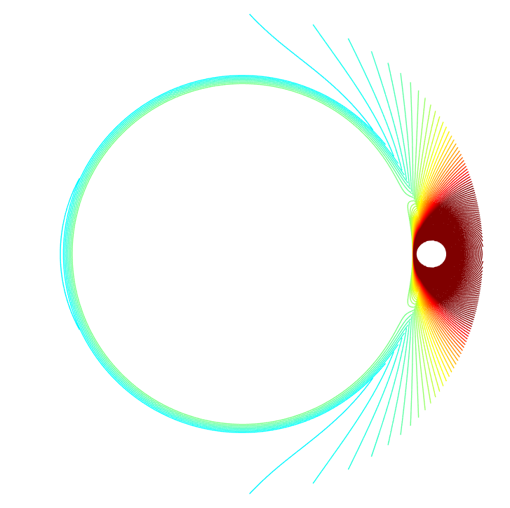
We can apply this formula concretely to the case of a radially-expanding disk. Suppose that $D_{0}$ is the unit disk, and set Q0s=Bs/Ο€superscriptsubscript𝑄0𝑠subscriptπ΅π‘ πœ‹Q_{0}^{s}=B_{\sqrt{s/\pi}} for $s\in[0,1)$. In this setting, we can imagine our source as a collection of outwardly moving rings of radius $0\leq r<1$, as shown in Figure 2. From symmetry considerations, it is clear that Ds=B1+s/Ο€subscript𝐷𝑠subscript𝐡1π‘ πœ‹D_{s}=B_{\sqrt{1+s/\pi}} are outwardly expanding disks.

Refer to captionRefer to caption
Figure 2: An illustration of the flow $s\mapsto D_{s}$ in the case of a radially-expanding disk. Here, $D_{0}$ is the unit disk (cyan, left), and our single source set $Q_{0}^{T}$ is a smaller disk within it (red, left). As time passes, source points move from the center of $Q_{0}^{s}$ to the outer boundary of $D_{s}$.

Suppose $p$ and $q$ lie in the plane, on origin-centered circles of radii $1<r_{q}\leq r_{p}<\sqrt{2}$ and at polar angles $\theta_{p},\theta_{q}$. The functions $F_{p}$ and $F_{q}$ take the following forms:

$$F_{p}(re^{i\theta})=\sum_{n\in\mathbb{Z}}\left(r/r_{p}\right)^{|n|}e^{in(\theta-\theta_{p})},\qquad F_{q}(re^{i\theta})=\sum_{n\in\mathbb{Z}}\left(r/r_{q}\right)^{|n|}e^{in(\theta-\theta_{q})}.$$

Then, from Theorem 6.1, we can calculate

$\displaystyle g(p,q)$ $\displaystyle=\frac{1}{v_{p}v_{q}}\int_{0}^{r_{q}}rdr\int_{0}^{2\pi}d\theta\;F_{p}F_{q}(1-\sigma_{\pi(r_{q}^{2}-1)})$
$\displaystyle=(2\pi)^{2}r_{p}r_{q}\int_{0}^{r_{q}}dr\int_{0}^{2\pi}d\theta\;rF_{p}F_{q}(1-\sigma_{\pi(r_{q}^{2}-1)})$
$\displaystyle=(2\pi)^{2}r_{p}r_{q}\int_{0}^{r_{q}}dr\int_{0}^{2\pi}d\theta\;r\sum_{j,k\in\mathbb{Z}}\frac{r^{|j|+|k|}}{r_{p}^{|j|}r_{q}^{|k|}}e^{i(j+k)\theta-ij\theta_{p}-ik\theta_{q}}(1-\sigma_{\pi(r_{q}^{2}-1)}).$

Only the terms with $j+k=0$ survive when integrating $\theta$:

$\displaystyle g(p,q)$ $\displaystyle=(2\pi)^{3}r_{p}r_{q}\int_{0}^{r_{q}}dr\;\sum_{j\in\mathbb{Z}}\frac{r^{2|j|+1}}{r_{p}^{|j|}r_{q}^{|j|}}e^{ij(\theta_{p}-\theta_{q})}(1-\sigma_{\pi(r_{q}^{2}-1)}).$

Now, we break this into two integrals using $\sigma_{\pi(r_{q}^{2}-1)}=\mathbf{1}_{\{r\leq\sqrt{r_{q}^{2}-1}\}}+\mathbf{1}_{\{r\leq 1\}}$:

$\displaystyle g(p,q)$ $\displaystyle=(2\pi)^{3}r_{p}r_{q}\int_{1}^{r_{q}}dr\;\sum_{j\in\mathbb{Z}}\frac{r^{2|j|+1}}{r_{p}^{|j|}r_{q}^{|j|}}e^{ij(\theta_{p}-\theta_{q})}-(2\pi)^{3}r_{p}r_{q}\int_{0}^{\sqrt{r_{q}^{2}-1}}dr\;\sum_{j\in\mathbb{Z}}\frac{r^{2|j|+1}}{r_{p}^{|j|}r_{q}^{|j|}}e^{ij(\theta_{p}-\theta_{q})}$
$\displaystyle=(2\pi)^{3}r_{p}r_{q}\sum_{j\in\mathbb{Z}}\frac{e^{ij(\theta_{p}-\theta_{q})}}{r_{p}^{|j|}r_{q}^{|j|}}\left(\int_{1}^{r_{q}}r^{2|j|+1}dr-\int_{0}^{\sqrt{r_{q}^{2}-1}}r^{2|j|+1}dr\right)$
$\displaystyle=(2\pi)^{3}r_{p}r_{q}\sum_{j\in\mathbb{Z}}\frac{1}{2|j|+2}\frac{e^{ij(\theta_{p}-\theta_{q})}}{r_{p}^{|j|}r_{q}^{|j|}}\left(r_{q}^{2|j|+2}-1-(r_{q}^{2}-1)^{|j|+1}\right).$

We can discard the negative frequency modes by rewriting this sum as twice the real part of its positive frequency modes:

$\displaystyle g(p,q)$ $\displaystyle=(2\pi)^{3}(r_{p}r_{q})^{2}\operatorname{Re}\left(\sum_{j=0}^{\infty}\frac{1}{j+1}\frac{e^{ij(\theta_{p}-\theta_{q})}}{r_{p}^{j+1}r_{q}^{j+1}}\left(r_{q}^{2j+2}-1-(r_{q}^{2}-1)^{j+1}\right)\right)$
$\displaystyle=(2\pi)^{3}(r_{p}r_{q})^{2}\operatorname{Re}\left(e^{-i(\theta_{p}-\theta_{q})}\sum_{j=0}^{\infty}\frac{1}{j+1}e^{i(j+1)(\theta_{p}-\theta_{q})}\left(\frac{r_{q}^{j+1}}{r_{p}^{j+1}}-\frac{1}{r_{p}^{j+1}r_{q}^{j+1}}-\frac{(r_{q}^{2}-1)^{j+1}}{r_{p}^{j+1}r_{q}^{j+1}}\right)\right)$
$\displaystyle=-(2\pi)^{3}(r_{p}r_{q})^{2}\operatorname{Re}\bigg{[}e^{-i(\theta_{p}-\theta_{q})}\bigg{(}\operatorname{Log}(1-e^{i(\theta_{p}-\theta_{q})}r_{q}/r_{p})-\operatorname{Log}(1-e^{i(\theta_{p}-\theta_{q})}1/r_{p}r_{q})$
$\displaystyle\hskip 238.49121pt-\operatorname{Log}(1-e^{i(\theta_{p}-\theta_{q})}(r_{q}^{2}-1)/r_{p}r_{q})\bigg{)}\bigg{]}$
$\displaystyle=-(2\pi)^{3}|pq|\operatorname{Re}\left[{\overline{p}}q\big{(}\operatorname{Log}(1-{\overline{q}}/{\overline{p}})-\operatorname{Log}(1-1/{\overline{p}}q)-\operatorname{Log}(1-(|q|^{2}-1)/{\overline{p}}q)\big{)}\right],$

where $\operatorname{Log}$ denotes the principle value of the logarithm, and we view $p$ and $q$ as complex numbers. This function is plotted in Figure 3.
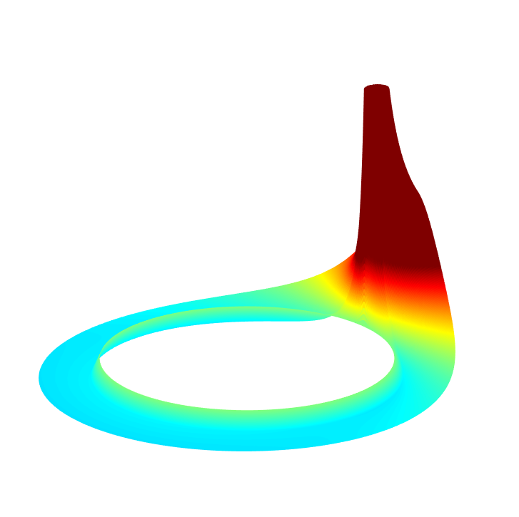
Refer to caption
Refer to caption
Figure 3: A plot and contour map of the function $g(p,q)$, where $q=(\nicefrac{{1}}{{2}}+\nicefrac{{\sqrt{5}}}{{4}},0)$ is fixed. Note the logarithmic singularity at $p=q$, and that the function vanishes for $p$ along the unit circle (the inner boundary of the domain).

The function $g(p,q)$ has several key properties, which we can see in Figure 3. For one, $g(p,q)$ is positive if and only if $\theta_{p}$ and $\theta_{q}$ are nearby. This confirms the geometric intuition that, for instance, an early point leads to other nearby early points, but that it prevents distant early points (by using up particle mass itself). Secondly, $g(p,q)$ vanishes as either $p$ or $q$ approaches the unit disk, likely reflecting the fact that points nearer to $D_{0}$ are β€œmore deterministic”—i.e., that the variance of their lateness decreases to 0 as they get closer to $D_{0}$. It is easy to check from Theorem 6.1 that this property holds true for other flows, as well, with the unit disk replaced by $D_{0}$ in general.

Next, note the logarithmic singularity present at $p=q$. This is to be expected, in analogy to the (free space) Green’s function $G(x,y)=\log|x-y|$. Indeed, just as we can view the Green’s function as giving an inner product

$$(u,v)_{-1}:=\int dxdy\;u(x)G(x,y)v(y)=\int dy\;(\nabla^{-2}u)(y)v(y),$$

we can view the point-correlation function $g$ as the kernel of the inner product defined in Equation 3:

$$(u,v)_{g}:=\int dxdy\;u(x)g(x,y)v(y)=\int_{0}^{T}ds^{\prime}\int_{0}^{s^{\prime}}ds^{\prime\prime}\int_{D_{s^{\prime\prime}}}(\psi_{s^{\prime}}\varphi_{s^{\prime\prime}}+\psi_{s^{\prime\prime}}\varphi_{s^{\prime}})(1-\sigma_{s^{\prime\prime}}),$$

where, as before, ψssubscriptπœ“π‘ \psi_{s} and Ο†ssubscriptπœ‘π‘ \varphi_{s} are the solutions of the Dirichlet problem on $D_{s}$ for $u$ and $v$, respectively.

7 Directions for further research

One interesting extension of this work would be to extend these results to higher dimensions. In dimension $d$, the appropriate scaling factor for the fluctuation functions EmssubscriptsuperscriptπΈπ‘ π‘šE^{s}_{m} and LmssubscriptsuperscriptπΏπ‘ π‘šL^{s}_{m} would be $m^{d/2}$ (just as it is $m=m^{2/2}$ here). In general, then, the error found in (5) and (8) would come out to be $O(m^{d/2}\varepsilon_{m}^{2})$. For this to decrease, we then need the bound $\varepsilon_{m}=o(m^{-d/4})$ on the maximum fluctuations. This is likely possible to achieve if $d=3$, but clearly impossible for $d\geq 4$.

However, there are weaker results that remain possible for $d\geq 4$. For one, if we require the test function $u$ to be harmonic, then we could achieve $\|u-\psi_{(m)}\|_{\infty}=O(m^{-2})$ on the domain of interest, rather than our existing $\|u-\psi_{(m)}\|_{\infty}=O(\varepsilon_{m})$. In this case, the requirement on $\varepsilon_{m}$ becomes $\varepsilon_{m}=o(m^{2-d/2})$, which now appears possible for dimensions 4 and 5.

Another important direction of research would be to generalize the sorts of possible sources for IDLA. For instance, it would be interesting to see if corresponding scaling limits hold if, instead of starting from a concentrated mass distribution, we were to start points evenly from a submanifold of $D_{0}$. Starting from the boundary of $D_{0}$, for example, may provide a good substitute for starting particles evenly across $D_{0}$ itself. In chemical applications, this adjusted setting could model a solid particle source of a particular shape.

Fortunately, the methods used in this paper translate fairly straightforwardly to other settings. The greatest obstacle to generalizing our results is finding an analogue to Lemma 2.4, which was the primary result of the preceding paper [Dar20]. Indeed, if it could be shown that the fluctuations of IDLA from a particular source satisfy a similar $O(m^{-1/2-\varepsilon})$ bound (for any $\varepsilon>0$), the remainder of our argument could likely be repeated.

A Appendix: maximum fluctuations of the divisible sandpile

We will use the capital $N_{m}(t)$ to denote the fully occupied set

$$N_{m}(t):=\{\nu_{m,t}=1\}\subset\frac{1}{m}\mathbb{Z}^{2}.$$

We will also use the notation of [Dar20]β€”in particular, for any $\zeta\in\frac{1}{m}\mathbb{Z}^{2}\setminus D_{0}$, we will write $\tau=\tau(\zeta)$ for the time at which $\zeta\in\partial D_{\tau}$, and we will use $H_{\zeta}$ and $\Omega_{\zeta}$ exactly as in that paper. We will not give more details on these objects here.

Now, we say that a point $z\in\frac{1}{m}\mathbb{Z}^{2}$ is $\varepsilon$-early at time $t$ if $z\in N_{m}(t)$, but $z\notin(D_{t/m^{2}})^{\varepsilon}$. Similarly, $z$ is $\varepsilon$-late at time $t$ if $z\in(D_{t/m^{2}})_{\varepsilon}$, but $z\notin N_{m}(t)$.

Finally, we will define a stopped version of $\nu_{m,t}$, as follows:

Definition A.1 (Stopped Sandpile).

Given $\nu_{\zeta,n}$, define the intermediate function $\nu_{\zeta,n}^{0}=\nu_{\zeta,n}+\mathbf{1}_{\{z_{m,n+1}\}}$. At each time step $t$, choose a point $z=z(t)\in\operatorname{supp}\nu_{\zeta,n}^{t}\setminus\partial D_{\tau}$ such that $\nu_{\zeta,n}^{t}(z)>1$. Let Wm,nt​(s)superscriptsubscriptπ‘Šπ‘šπ‘›π‘‘π‘ W_{m,n}^{t}(s) be a Brownian motion started from $z$ on the grid

$$\mathcal{G}_{m}:=\left\{(x,y)\in\mathbb{R}^{2}\;\bigg{|}\;x\in\frac{1}{m}\mathbb{Z}^{2}\;\text{or}\;y\in\frac{1}{m}\mathbb{Z}^{2}\right\},$$

as defined in Definition 4.3 of [Dar20]. Define the stopping time

Ο„βˆ—:=inf{s|Wm,nt​(s)∈(1m​℀2βˆ–Nm​(n))βˆͺβˆ‚DΟ„},assignsuperscript𝜏infimumconditional-set𝑠superscriptsubscriptπ‘Šπ‘šπ‘›π‘‘π‘ 1π‘šsuperscriptβ„€2subscriptπ‘π‘šπ‘›subscript𝐷𝜏\tau^{*}:=\inf\left\{s\;\bigg{|}\;W_{m,n}^{t}(s)\in\left(\frac{1}{m}\mathbb{Z}^{2}\setminus N_{m}(n)\right)\cup\partial D_{\tau}\right\},

and set

$$\nu_{\zeta,n}^{t+1}(z^{\prime})=\nu_{\zeta,n}^{t}(z^{\prime})+(\nu_{\zeta,n}^{t}(z)-1)\cdot\left(\mathbb{P}\left[W_{m,n}^{t}(\tau^{*})=z\right]-\delta_{z,z^{\prime}}\right).$$

For a large enough $t^{\prime}$, we have that $\nu_{\zeta,n}^{t^{\prime}}(z)\leq 1$ everywhere in $\operatorname{supp}\nu_{m,n}^{t^{\prime}}\setminus\partial D_{\tau}$; then we define $\nu_{\zeta,n+1}=\nu_{\zeta,n}^{t^{\prime}}$.

In parallel with the original divisible sandpile model, we define $\nu_{\zeta,n+1}$ by taking the excess mass at $z$ in $\nu_{\zeta,n}$ and splitting it around the edge of $\operatorname{supp}\nu_{\zeta,n}$ according to a discrete harmonic measure. New in this case, however, is that we stop mass before it exits the domain $D_{\tau}$.

Note that this satisfies the same key equality as the original harmonic measure; namely, for any grid harmonic (see [Dar20]) $H$ defined in $\frac{1}{m}\mathbb{Z}^{2}\cap D_{\tau}$,

$$\sum H\cdot\left(\nu_{\zeta,t}-\sigma_{\zeta,t}\right)=0.$$
Lemma A.2 (Thin Tentacles).

There is an absolute constant $b>0$ such that for all $z\in A_{m}(t)\subset\frac{1}{m}\mathbb{Z}^{2}$ with $d(z,D_{0})\geq r$,

$$\#\left(N_{m}(t)\cap B(z,r)\right)>bm^{2}r^{2}.$$
Proof.

For this, we define the intermediate processes $\nu_{m,t}^{\ell}$, for each integer $\ell\geq 1$:

  1. 1.

    Define the initial set $\nu^{\ell}_{m}(0)=\nu_{m}(0)=\mathbf{1}_{\frac{1}{m}\mathbb{Z}^{2}\cap D_{0}}$.

  2. 2.

    For each $i\in\frac{1}{\ell}\mathbb{Z}_{>0}$, start a random walk at $z_{m,\lceil i\rceil}$, and let $z^{\prime}_{i}$ be the first point in the walk at which $\nu^{\ell}_{m,i-\ell^{-1}}(z^{\prime}_{i})<1$. Let $\nu^{\ell}_{m,i}=\nu^{\ell}_{m,i-\ell^{-1}}+\ell^{-1}\mathbf{1}_{\{z_{i}^{\prime}\}}$.

Now, $\nu_{m,t}^{0}$ is simply an IDLA, by definition, and $\nu_{m,t}^{\ell}\to\nu_{m,t}$ in law (pointwise) in $\ell$. We can now lift the proof of Lemma 2 of [JLS12] (Lemma 3.2 of [Dar20]) verbatim,222The only significant difference in proving the new result is that the total number of β€œtrials”, as well as the total number of required β€œfailures” (in the language of [JLS12]), is scaled up by a factor of $\ell$. to show that

$$\mathbb{P}\left[\nu^{\ell}_{m,t}(z)>0,\#\left(\{\nu^{\ell}_{m,t}=1\}\cap B(z,r)\right)\leq bm^{2}r^{2}\right]\leq C_{0}e^{-c_{0}mr}$$

for constants $c_{0},C_{0}$ independent of $\ell$. In particular, this probability is uniformly bounded below 1 in $\ell$; since $\nu_{m,t}^{\ell}$ converges in law to the deterministic function $\nu_{m,t}$, we see that

$$\lim_{\ell\to\infty}\mathbb{P}\left[\nu^{\ell}_{m,t}(z)>0,\#\left(\{\nu^{\ell}_{m,t}=1\}\cap B(z,r)\right)\leq bm^{2}r^{2}\right]=0,$$

from which the lemma follows. ∎

The next theorem is a restatement of Theorem 2.7, and a stronger version of Theorem 3.9 of [LP08]:

Theorem A.3 (Theorem 2.7).

There is a constant $C>0$ dependent on the flow such that, for large enough $m$ and any $s\in[0,T]$,

$$\frac{1}{m}\mathbb{Z}^{d}\cap(D_{s})_{Cm^{-3/5}}\subset N_{m}(m^{2}s)\subset(D_{s})^{Cm^{-3/5}}.$$
Lemma A.4.

There are constants $C,\alpha>0$ dependent only on the flow such that, for large enough $m$, $s\in[0,T]$, $a\geq Cm^{2/5}$, and $\ell\leq\alpha a$, an $a/m$-early point in $N_{m}(t)$ by time $m^{2}s$ implies a different, $\ell/m$-late point by time $m^{2}s$.

Proof.

Suppose $z\in N_{m}(t)\setminus N_{m}(t-1)$ is the first $a/m$-early point in $N_{m}$β€”that is, $z\notin(D_{t/m^{2}})^{a/m}$, but $N_{m}(t-1)\subset(D_{(t-1)/m^{2}})^{a/m}$. Further assume that there are no $\ell/m$-late points by the time $t$, or equivalently that $(D_{t/m^{2}})_{\ell/m}\subset N_{m}(t)$.

Since $z$ is adjacent to $N_{m}(t-1)$, we know that

$$N_{m}(t)\subset(D_{t/m^{2}})^{(a+1)/m}.$$

Let $\zeta=\zeta(z,t)$ be the nearest point to $z$ in the annulus

$$\frac{1}{m}\mathbb{Z}^{2}\cap(D_{t/m^{2}})^{V(4a+2C)/mv+2/m}\setminus(D_{t/m^{2}})^{V(4a+2C)/mv},$$

where $C$ will be specified later, and $v,V>0$ are as in Lemma 3.5 of [Dar20]. Let $\tau>0$ be such that $\zeta\in\partial D_{\tau}$, and note that

$$d_{H}(D_{t/m^{2}},D_{\tau})\geq d(D_{t/m^{2}},\zeta)\geq V(4a+2C)/mv.$$

By Lemma 3.5 of [Dar20], this implies

$\displaystyle d(N_{m}(t),D_{\tau}^{c})$ $\displaystyle\geq d((D_{t/m^{2}})^{(a+1)/m},D_{\tau}^{c})$
$\displaystyle\geq d(D_{t/m^{2}},D_{\tau}^{c})-(a+1)/m$
$\displaystyle\geq\frac{v}{V}d_{H}(D_{t/m^{2}},D_{\tau})-(a+1)/m$
$\displaystyle\geq(3a+2C-1)/m>1.$

From Lemma 4.2(a) of [Dar20], this means $\operatorname{supp}(\nu_{m,t})\subset\Omega_{\zeta}$, and thus we can replace $\nu_{m,t}$ with $\nu_{\zeta,t}$. As in [Dar20], we can show thatβ€”if $\#\left(N_{m}(t)\cap B(z,a/m)\right)>ba^{2}$ and no points are $\ell/m$-late by time $t$β€”then

$$\sum_{z^{\prime}\in\frac{1}{m}\mathbb{Z}^{2}}\left(\nu_{\zeta,t}(z^{\prime})-\sigma_{m,t}(z^{\prime})\right)H_{\zeta}(z^{\prime})\geq vba/12V>0.$$

Both of the listed assumptions are true; we know $\#\left(N_{m}(t)\cap B(z,a/m)\right)>ba^{2}$ by Lemma A.2, and we have assumed that no points are $\ell/m$-late by time $t$. However, $\sum\left(\nu_{\zeta,t}-\sigma_{m,t}\right)H=0$ for any $H$ harmonic on $\operatorname{supp}(\nu_{\zeta,t})$, so this is a contradiction. ∎

Lemma A.5.

There is a constant $C>0$ dependent only on the flow such that, for large enough $m$, $s\in[0,T]$, and $\ell\geq Cm^{2/5}$, there can be no $\ell/m$-late point by time $m^{2}s$.

Proof.

Without loss of generality, let $a=\ell^{2}/Cm^{2/5}\geq\ell$. Fix an integer $t\leq m^{2}s$, and suppose that $\zeta\in\frac{1}{m}\mathbb{Z}^{2}\cap\left((D_{t/m^{2}})_{\ell/m}\setminus D_{0}\right)$ is $\ell/m$-late by time $t$. Then $d(\zeta,\partial D_{t/m^{2}})\geq\ell/m$, so by Lemma 3.5 of [Dar20],

$\displaystyle t-m^{2}\tau\geq 2m^{2}\sqrt{1+\tau}$ $\displaystyle\left(\sqrt{1+t/m^{2}}-\sqrt{1+\tau}\right)$
$\displaystyle\geq\frac{2m^{2}}{V}\sqrt{1+\tau}\cdot d_{H}(D_{t/m^{2}},D_{\tau})\geq\frac{2m^{2}}{V}\sqrt{1+\tau}\cdot d(\zeta,\partial D_{t/m^{2}})\geq\frac{2m\ell}{V}.$

Since $\zeta$ is $\ell/m$-late at time $t$, we know that $\zeta\notin N_{m}(t)$, so $\nu_{\zeta,t}(\zeta)<1$. As in [Dar20], the sum

$$\tilde{M}_{\zeta}(t):=\sum\nolimits_{z^{\prime}}\left(\nu_{\zeta,t}(z^{\prime})-\sigma_{m,t}(z^{\prime})\right)H_{\zeta}(z^{\prime})$$

is maximized if the interior of $\tilde{\Omega}_{\zeta}\cap\frac{1}{m}\mathbb{Z}^{2}$ is fully occupied by $N_{m}(t)$. We can then show, exactly as in [Dar20], that

$$\tilde{M}_{\zeta}(t)<1-c\ell$$

for some $c>0$; the new constant term comes from the $\nu_{\zeta,t}(\zeta)H_{\zeta}(\zeta)<1$ contribution. So long as $C$ is large enough, this is still negative; of course, we know that $\tilde{M}_{\zeta}(t)=0$, so this is a contradiction. ∎

Proof of Theorem 2.7.

We can work with the set $N_{m}(t)$ instead of $\operatorname{supp}\nu_{m,t}$; indeed, the latter only differs from the former within one unit of the boundary. By Lemma A.5, we only need to show that no $O(m^{-3/5})$-early point can exist. Suppose a point is $\alpha^{-1}Cm^{-3/5}$-early at a time $t\leq m^{2}s$. By Lemma A.4, this implies that another point is $Cm^{-3/5}$-late by the same time; this contradicts Lemma A.5, and we retrieve our result. ∎

Acknowledgments

I would like to thank Professor David Jerison and Pu Yu (MIT Department of Mathematics) for their mentorship throughout this project, as well as Professor Scott Sheffield for his insights regarding the divisible sandpile model.

References

  • [AG10] Amine Asselah and Alexandre GaudilliΓ¨re. A note on fluctuations for internal diffusion limited aggregation, 2010. Available at https://arxiv.org/abs/1004.4665.
  • [AG11] Amine Asselah and Alexandre GaudilliΓ¨re. Lower bounds on fluctuations for internal DLA, 2011.
  • [AG13a] Amine Asselah and Alexandre GaudilliΓ¨re. From logarithmic to subdiffusive polynomial fluctuations for internal DLA and related growth models. Ann. Probab., 41(3A):1115–1159, 05 2013.
  • [AG13b] Amine Asselah and Alexandre GaudilliΓ¨re. Sublogarithmic fluctuations for internal dla. The Annals of Probability, 41(3A):1160–1179, May 2013.
  • [Che] Long Chen. Finite difference methods for poisson equation. Available at https://www.math.uci.edu/~chenlong/226/FDM.pdf.
  • [Dar20] David Darrow. A convergence rate for extended-source internal DLA in the plane, 2020. Available at https://arxiv.org/abs/2009.09159.
  • [DF91] P.Β Diaconis and W.Β Fulton. A Growth Model, a Game, an Algebra, Lagrange Inversion, and Characteristic Classes. Stanford University, Department of Statistics, 1991.
  • [HH80] P.Β Hall and C.C. Heyde. Chapter 3 - the central limit theorem. In Martingale Limit Theory and its Application, pages 51 – 96. Academic Press, 1980.
  • [JLS12] David Jerison, Lionel Levine, and Scott Sheffield. Logarithmic fluctuations for internal DLA. Journal of the American Mathematical Society, 25(1):271–301, 2012.
  • [JLS13] David Jerison, Lionel Levine, and Scott Sheffield. Internal DLA in higher dimensions. Electron. J. Probab., 18:14 pp., 2013.
  • [JLS14] David Jerison, Lionel Levine, and Scott Sheffield. Internal DLA and the Gaussian free field. Duke Math. J., 163(2):267–308, 02 2014.
  • [Law95] GregoryΒ F. Lawler. Subdiffusive fluctuations for internal diffusion limited aggregation. Ann. Probab., 23(1):71–86, 01 1995.
  • [LBG92] GregoryΒ F. Lawler, Maury Bramson, and David Griffeath. Internal diffusion limited aggregation. Ann. Probab., 20(4):2117–2140, 10 1992.
  • [LP08] Lionel Levine and Yuval Peres. Strong spherical asymptotics for rotor-router aggregation and the divisible sandpile. Potential Analysis, 30(1):1–27, Oct 2008.
  • [LP10] Lionel Levine and Yuval Peres. Scaling limits for internal aggregation models with multiple sources. Journal d’Analyse MathΓ©matique, 111(1):151–219, May 2010.
  • [MD86] Paul Meakin and J.Β M. Deutch. The formation of surfaces by diffusion limited annihilation. The Journal of Chemical Physics, 85(4):2320–2325, 1986.
  • [Sad16] Eli Sadovnik. A central limit theorem for fluctuations of internal diffusion-limited aggregation with multiple sources, 2016. Available at https://math.mit.edu/research/undergraduate/urop-plus/documents/2016/Sadovnik.pdf.