An updated detailed characterization of planes of satellites in the MW and M31

Abstract

We present a detailed characterization of planes of satellite galaxies in the Milky Way (MW) and M31. For a positional analysis, we introduce an extension to the ‘4-galaxy-normal density plot’ method (Pawlowski et al., 2013, P13). It finds the normal directions to the predominant planar configurations of satellites of a system, yielding for each a collection of planes of increasing member satellites. This allows to quantify the quality of planes in terms of population ($N_{\rm sat}$) and spatial flattening ($c/a$). We apply this method to the latest data for confirmed MW and M31 satellite samples, with 46 and 34 satellites, respectively. New MW satellites form part of planes previously identified from the sample with $N_{\rm sat}=27$ studied in P13: we identify a new plane with $N_{\rm sat}=39$ as thin as the VPOS-3 ($c/a\sim 0.2$), and with roughly the same normal direction; so far the most populated plane that thin reported in the Local Group. We introduce a new method to determine, using kinematic data, the axis of maximum co-orbitation of MW satellites. Interestingly, this axis approximately coincides with the normal to the former plane: $\geq 45\pm 5\%$ of satellites co-orbit. In M31 we discover a plane with $N_{\rm sat}=18$ and $c/a\sim 0.15$, i.e., quality comparable to the GPoA, and perpendicular to it. This structure is viewed face-on from the Sun making it susceptible to M31 satellite distance uncertainties. An estimation of the perpendicular velocity dispersion suggests it is dynamically unstable. Finally we find that mass is not a property determining a satellite’s membership to good quality planes.

1 Introduction

The known objects surrounding the Milky Way (MW) show an anisotropic spatial distribution. Lynden-Bell (1976) and Kunkel & Demers (1976) were the first to notice that dSphs Sculptor, Draco, Ursa Minor and globular cluster Palomar 13, apparently lied on the orbital plane of the Magellanic stream, therefore polar to the Galaxy. Soon after, Fornax, Leo I, Leo II, Sextans, Phoenix and some classified as ‘young halo’ globular clusters, were also found to participate of this “great circle” (Lynden-Bell, 1982; Majewski, 1994; Fusi Pecci et al., 1995). The existence of a “plane of satellites” in the MW was finally ratified when measuring the very flattened distribution of the 11 classical satellites as compared to isotropy (Kroupa et al., 2005; Metz et al., 2007). In our neighboring galactic system Andromeda (M31), the first studies by Grebel et al. (1999) and Koch & Grebel (2006) on the then-known $\lesssim$15 dwarf galaxies within $\sim$500 kpc distance, found that the subsample of dSph/dE type dwarfs also lied near a “great circle”. This spatial anisotropy was emphasized by the skewness of M31 dwarfs in the direction to the MW (McConnachie & Irwin, 2006). More recently, the addition to the picture of newly discovered faint satellites thanks to surveys like SDSS (York et al., 2000) or PAndAS (McConnachie et al., 2009), and an increased quality of distance measurements, has only enhanced the significance of the planar structures noted in the MW and M31 (Metz et al., 2009; Kroupa et al., 2010; Ibata et al., 2013; Conn et al., 2013; Pawlowski et al., 2013; Pawlowski & Kroupa, 2014; Pawlowski et al., 2015). In addition, a richer census of young halo globular clusters and several stellar/gaseous streams have been shown to also align with the MW satellites (Keller et al., 2012; Pawlowski et al., 2012; Riley & Strigari, 2020). Finally, apart from the MW and M31, there are claims for a planar distribution of satellites in the nearby Centaurus A Group of galaxies (Tully et al., 2015), further supported by discoveries of new dwarfs and better distance estimates (Müller et al., 2016, 2018).

In the last years, the quantification of such planar alignments has gained increasing importance in order to unambiguously define the observed structures in terms of their orientation and characteristics. These quantifications have demanded increasingly more sophisticated methods that make use of the three-dimensional position data as well as statistical approaches to overcome measurement uncertainties or avoid spurious effects coming from working with a small sample number.

Specifically, Koch & Grebel (2006) used an error-weighted orthogonal distance regression accompanied by bootstrapped tests, to reliably determine a robust solution for estimating best-fit planes. They fitted a plane to all possible subsamples of M31 satellites involving 3 to 15 members and projected the resulting normal vectors on a sphere. With the density distribution of normals they found an estimation of the normal direction to the broad planar distribution defined by the satellites’ positions. Metz et al. (2007, 2009) used instead the Tensor of Inertia plane-fitting method taking into account distance uncertainties. More recently, Pawlowski et al. (2013), (hereafter P13), combined the previous efforts and presented a new statistical method to define the direction of predominant plane-like spatial distributions of satellites within a given sample: the ‘4-galaxy-normal density plot’ method, consisting of a planar fit to every combination of 4 satellites. From its application to the confirmed satellites within 300 kpc in the MW and M31 at that time, they found one predominant planar alignment of satellites in each galactic system and measured their respective normal directions. In this way, the so-called “VPOS-3” (Vast Polar Structure) in the MW and “GPoA” (Great Plane of Andromeda) in M31 planes were defined, consisting of 24 and 19 satellites respectively. These planes have been considered so far to be the most relevant satellite planar configurations in the MW and M31, and have been used as a benchmark against which to test the alignment of the newest (some even of unclassified nature) objects discovered (Pawlowski & Kroupa, 2014; Pawlowski et al., 2015).

However, a detailed characterization of these predominant planar structures in the MW and M31, finding which are the combinations of $N_{\rm sat}$ satellites out of a total sample $N_{\rm tot}$ that conform the most relevant planar structures, is still lacking. Moreover, it is of interest to highlight those specific planes of satellites within a system with highly striking characteristics. This identification demands an analysis of how the quality of these planes changes with the number of satellites involved.

This paper is the first of a series where the results of a project aimed at working in depth the plane of satellites issue within a $\Lambda$CDM  cosmological context are reported. The purpose of this paper is to present a more detailed quantification and characterization of the plane-like spatial structures in the MW and M31 satellite systems. This is an important issue and, additionally, it will provide a reference with which to compare results from analyses of numerical simulations of the formation of disc galaxy systems (Santos-Santos et al., 2020, hereafter Paper II). We focus on the positions of satellites, which for the MW have error bars much smaller than those of kinematic data. We note, however, that complementary, relevant information to satellite planar alignments comes from kinematic data. Indeed, recent proper motions for MW satellites measured with Gaia (see e.g., Gaia Collaboration et al., 2018; Fritz et al., 2018; Simon, 2018) suggest that a non-negligible fraction of them are orbiting along the VPOS plane (Fritz et al., 2018) while others are most likely not associated to the structure as their orbital poles are not aligned with the VPOS normal vector (see e.g., Pawlowski & Kroupa, 2020, for a recent study of the classical MW satellites). To study the reproducibility of these results in numerical simulations, in Santos-Santos et al. (in preparation, hereafter Paper III) we develop in depth the so-called ‘3J_orb-barycenter’ method, and apply it to zoom-in simulations of disc galaxies. This method identifies the axes around which a maximum number of satellites, out of a given population, co-orbit; allowing the study of relevant issues such as plane persistence along galaxy evolution.

In this paper we build on the results of P13 and develop an extension to the ‘4-galaxy-normal density plot’ method that enables a deeper cataloguing and quality analyses of planes of satellites in a galactic system. In particular, for each predominant planar configuration of satellites in the MW and M31 found with the previous method, we yield a collection of planes of increasing $N_{\rm sat}$ satellite members, and we identify the highest-quality ones in terms of the Tensor of Inertia parameters and the number of satellites involved. In particular, a plane’s quality is quantified in terms of its population ($N_{\rm sat}$) and flattening (the concentration ellipsoid short-to-long axis ratio $c/a$ or, equivalently, the r.m.s. thickness normal to the plane; Cramér 1999). Quality of planes with the same population or flattening can be compared with each other, allowing to single-out high quality planes with the same $N_{\rm sat}$ or $c/a$ values.

Finally, to complete the analyses of positionally-identified planes of satellites in the MW, we briefly study here their kinematically-coherent character, and independently, identify the MW’s maximum satellite co-orbitation axis through the ‘3J_orb-barycenter’ method mentioned above. For M31 satellites only line-of-sight velocities are currently available (Ibata et al., 2013) and such a study is not possible yet. In addition, distances to M31 satellites remain highly uncertain (see e.g. Weisz et al., 2019).

The paper is organized as follows. In Section 2 we present the samples and datasets of MW and M31 satellites studied. In Section 3 we thoroughly describe our methodology for plane-searching from satellite position data. Sections 4 and 5 show the results of our quality analysis for planes in the MW and M31, respectively. The co-orbitation issue and the determination of the axes of maximum rotation in the MW are addressed in Section 6. Finally, Section 7 summarizes our conclusions.

2 MW and M31 data

In this project, we analyze planes of satellites in samples of $N_{\rm tot}$ confirmed satellite (i.e., bound to the MW or M31 hosts) galaxies (i.e., not other objects such as globular clusters or streams have been considered).

For the MW we use two different satellite samples. First, for the sake of consistency with P13, and for simplicity as far as comparisons are concerned (see e.g. Pawlowski, 2016), we analyze the same satellite sample as in P13 consisting of $N_{\rm tot}=27$ satellites. This satellite sample will be hereafter termed ’MW27 sample’ and it consists of the classical and SDSS satellites. MW27 lists all the satellites within 300 kpc from the MW, according to the McConnachie (2012) “Nearby dwarf galaxy database” as of June 2013. Most probable satellite position values and their corresponding Gaussian width uncertainties in the radial Sun - satellite distance have been taken from this database, as summarized in table 2 of P13. Canis Major and BootesIII are considered in MW27 as dwarf galaxies although their nature as such is ruled out (see Momany et al., 2004; Martínez-Delgado et al., 2005; Mateu et al., 2009), and debated (see Grillmair, 2009; Carlin & Sand, 2018), respectively.

On top of this historical sample, we also analyze an up-to-date (as of August 2020) sample of all confirmed MW satellite galaxies, consisting of $N_{\rm tot}=46$ satellites; hereafter ’MW46’. The MW46 sample includes 25 satellites in common with MW27 (Canis Major and BootesIII are not included as they are of doubtful nature, see above), and 21 new ones. These are recently discovered ultrafaint satellite galaxies within a radial distance of 300 kpc from the MW center which originate from a variety of sources/surveys (e.g. The Dark Energy Survey, DECam surveys like Maglites, DELVE, ATLAS, Subaru/Hyper Suprime-Cam Survey, Gaia Bechtol et al., 2015; Koposov et al., 2015; Drlica-Wagner et al., 2015; Homma et al., 2016; Torrealba et al., 2016, 2019; Mau et al., 2020). In particular, here we consider as ”confirmed” ultrafaint MW satellites those objects that are either spectroscopically confirmed (see Simon, 2019), or, alternatively, that populate the dwarf galaxy parameter space of the $M_{V}$-r_half plane (relation between absolute V magnitude and half-light radius of the object), in opposition to the globular cluster regime (note this is only possible to assess in the cases where r_half data is available). These 21 objects are: Tucana2, Hydra2, Hydrus1, Carina2, Pictor2, Virgo1, Aquarius2, Crater2, Antlia2, BootesIV, Cetus3, HorologiumI, ReticulumII, PegasusIII, Tucana4, Columba1, Grus2, PheonixII, HorologiumII, ReticulumIII, Centaurus1. In Appendix A we present Table 4 with the positions (RA, dec), distances from the Sun and stellar masses of all MW satellites used in this paper.

As for M31, we use as reference the same satellite sample as in P13, consisting of 34 confirmed satellites within 300 kpc of the M31 center (hereafter M31_34, see McConnachie, 2012). As of August 2020, no new M31 confirmed satellites within 300 kpc have been added to those listed in P13’s table 2. For completeness, as the mass of M31 is estimated to be larger than that of the MW, and therefore M31 may present a larger virial radius, we have also considered in our analysis the case of extending the limiting distance to 350 kpc. This adds two extra satellites to the sample, AXVI and AXXXIII (also known as PerseusI), at $\sim 323$ and $\sim 346$ kpc from M31, respectively. We will refer to this extended sample as M31_36.

In Table 5 we list the M31 satellites included in our analysis and the data used: RA and dec positions, distances from the Sun, the references the distances assumed come from (with the specific distance determination method) and the stellar masses. Most heliocentric distances in this Table (as compiled in the database by McConnachie, 2012) are based on ground-based tip of the red giant branch (TRGB) calibration; however, in some cases they are not. We note that this may introduce a bias, as distances for the same object obtained with different methods have been shown to sometimes be very different (compare for example McConnachie et al., 2005; Conn et al., 2012; Weisz et al., 2019). In order to have results where the distance determinations are based on an homogeneous method, we have repeated the analyses with Conn et al. (2012) data (see their table 2), where distances for a long list of M31 satellites were obtained using the TRGB standard candle. In this case, for the 11 out of 36 M31 satellites that are not in Conn et al. (2012), distances in Table 5 have been used.

The different observational planes of satellites claimed in the literature which we will compare to are listed in Table 2 (see next section for definitions of plane properties). These were defined in P13 considering the MW27 and M31_34 samples of satellites. For the MW these planes are: the so-called ‘classical’ (i.e., the 11 most luminous MW satellites, see Metz et al., 2007), the ‘VPOSall’ (defined by all the 27 confirmed satellites within 300 kpc) and the ‘VPOS-3’ (defined by 24 out of 27 of the VPOSall satellites). For M31, there is the plane of satellites noted by Ibata et al. (2013) and Conn et al. (2013) with the PAndAS survey, which we will consider with 14 satellites (as analyzed in P13, hereafter the ‘Ibata-Conn-14’ plane) , and the so-called ‘GPoA’ with 19 members (the 14 of the ‘Ibata-Conn-14’ plane plus 5 more).

3 Planar configurations from position data

Our method to find planar structures and assess their quality consists of 2 parts. The first part follows the ’4-galaxy-normal density plot’ method described in Pawlowski et al. (2013). This technique checks if there is a subsample of a given satellite sample that defines a dominant planar arrangement in terms of the outputs of the standard Tensor of Inertia (ToI) plane-fitting technique (see Metz et al., 2007; Pawlowski et al., 2013), based on an orthogonal-distance regression. In terms of the corresponding concentration ellipsoid (Cramér, 1999), planes are characterized by:

• $N_{\rm sat}$: the number of satellites in the subsample;

• $\vec{n}$, the normal to the best fitting plane;

• $c/a$: the ellipsoid short-to-long axis ratio;

• $b/a$: the ellipsoid intermediate-to-long axis ratio;

• $\Delta$RMS: the root-mean-square thickness perpendicular to the best-fitting plane;

• $D_{\rm cg}$: the distance from the center-of-mass of the main galaxy to the plane.

These outputs are used to quantify the quality of planes. To begin with, a planar configuration must be flattened (i.e., low $c/a$), and, as opposed to filamentary, it also requires $b/a\sim 1$ for an oblate distribution. High quality planes are those with a high $N_{\rm sat}$, and a low $c/a$ and $\Delta$RMS, meaning they are populated and thin (plane quality as understood in this work will be specified in more detail at the end of the next section). Finally, a low $D_{\rm cg}$ means that the plane passes near the main galaxy’s center, a characteristic that dynamically stable planes must show, assuming that the host galaxy’s center is close to the center of the system’s gravitational potential well.

The second part of our methodology, which is the focus of this paper, is an extension to the 4-galaxy-normal density plot method, consisting of a quality analysis of the predominant planar arrangements found.

3.1 4-galaxy-normal density (4GND) plot method

This method was presented in sec. 2.4 of Pawlowski et al. (2013). We briefly summarize it and mention the procedure particularities followed in this study.

1. A plane is fitted to every combination of four satellites’ positions, using the ToI technique. The resultant normal vector (i.e. 4-galaxy-normal) and corresponding plane parameters are stored. To account for distance uncertainties, this step is repeated 100 times using 100 random positions per satellite, calculated using their corresponding radial distance uncertainties.

2. All the 4-galaxy-normals (from all 100 realizations) are projected on a regularly-binned sphere, assuming a Galactocentric coordinate system such that the MW’s disc spin vector points towards the south pole. A density map (i.e. 2D-histogram) is drawn from the projections, where each normal has been weighted by $\log\left(\frac{a+b}{c}\right)$ to emphasize planar-like spatial distributions. The over-density regions in these density maps (i.e. regions of 4-galaxy-normal accumulation) therefore signal the normal direction to a dominant planar space-configuration. Satellites contributing 4-galaxy-normals to a given over-density are likely members of such a dominant plane. As opposite normal vectors indicate the same plane, density maps in this study are shown through Aitoff spherical projection diagrams in Galactic coordinates (longitude $l$, latitude $b$) within the $l=[-90^{\circ},+90^{\circ}]$ interval.

3. We order bins by density value. The main over-density region is identified around the highest value bin. Subsequent over-densities are identified by selecting the next bin, in order of decreasing density, which is separated more than 15^∘ from the center of all the previously defined over-densities. In this way over-density regions are differentiated and isolated. For each of these regions, the midpoint of the highest-density bin will define the corresponding density peak’s coordinates.

4. We quantify how much a certain satellite $s$ has contributed to a given density peak $p$ (which we refer to as ’$C_{p,s}$’). To this end, we define an aperture angle of 15^∘ around the density peak, selecting all 4-galaxy-normals within it. For each of them, the four contributing satellites are determined. A given satellite $s$ is counted to contribute the 4-galaxy-normal’s weight to peak $p$. Therefore, its final contribution $C_{p,s}$, is the sum of weights corresponding to all the 4-galaxy-normals within the peak aperture that satellite $s$ contributes to. This has been normalized using $C_{N,all}$, the total weighted number of 4-galaxy-normals, included those that are not within 15^∘ of some peak center. Such normalization is necessary to allow for a meaningful comparison of results coming from samples with different sizes $N_{\rm tot}$.

   Finally, all satellites are ordered by decreasing $C_{p,s}$ to the density peak $p$, such that the first satellite is that which contributes most.

   We note that changing the bin size used in our analysis does not modify our results, as we find the same overdensity regions, and final order of satellites by $C_{p,s}$.

3.2 An extension to the method: peak strength and plane quality analysis

To allow an individual and in-depth analysis of each overdensity and its corresponding predominant planar structure of satellites, we present an extension of the 4-galaxy-normal density plot method.

On one hand, to each peak $p$ we assign a number, $C_{p}$, the peak ‘strength’, defined as the normalized number (or %) of 4-galaxy-normals within 15^∘ of the respective peak center; that is $C_{p}\equiv\sum_{s}C_{p,s}$, where the contribution-number $C_{p,s}$ of the $s$ satellite to the $p$-th peak has been defined above. This is a useful concept to quantify the comparisons of different density peaks and ultimately study the ‘relevance’ of given planar satellite structures over others (see Paper II for more details).

On another, rather than a plane per overdensity, the extended method provides a collection of planes, each consisting of a different number of satellites $N_{\rm sat}$.

For each over-density $p$ we initially fit a plane to the $N_{\rm sat}=7$ satellites with highest $C_{p,s}$ (i.e., the 7 satellites that contribute most to 4-galaxy-normals within 15^∘ of the density peak), and store the resultant plane parameters. This number $N_{\rm sat}=7$ is low enough to allow for an analysis of ToI parameter behaviour as $N_{\rm sat}$ increases, and at the same time high enough that we begin with populated planes. Note that taking instead $N_{\rm sat}=7\pm 2$ to begin with does not alter our conclusions.

Then, the next satellite in order of decreasing $C_{p,s}$ is added to the group of satellites. Again a plane is fitted to their positions and the parameters stored. This plane-fitting process is repeated until all contributing satellites are used.

To include the effect of distance uncertainties, in practice we calculate 1000 random positions per satellite, and fit 1000 planes at each iteration with $N_{\rm sat}$ satellites. The final results at each $N_{\rm sat}$ correspond to the mean values from these random realizations and the corresponding errors to the standard deviations.

In this way, for each over-density found we obtain a collection or catalog of planes of satellites, each plane consisting of a different number of members increasing from 7 to $N_{\rm tot}$, as well as the quality indicators for each of them.

In this work “high quality” means populated and flattened planes. This is quantified through $N_{\rm sat}$ and $c/a$ (and/or $\Delta$RMS, but note that they are very often correlated; see Pawlowski & McGaugh, 2014). Being a two-parameter notion, to compare planes’ qualities we need that either $N_{\rm sat}$ is constant or that $c/a$ is constant (or that at least it varies very slowly with $N_{\rm sat}$). In the first case, lower $c/a$ means higher quality. In the second case, more populated planes are rated as of higher quality. Another case when comparison is possible is when one plane is more flattened and populated than another: the first has a higher quality than the second. These considerations have been applied to the different member planes in the collection obtained for each density peak, allowing us to make quality comparisons, in particular with already determined planes, and, very interestingly, to single out new high-quality ones.

We finally note that the advantage of the 4GND plot method lies in that it selects the subsamples of $N_{\rm sat}$ satellites with lowest $c/a$ provided that they are embedded in an underlying more populated, predominant planar structure. In the case of low $N_{\rm sat}$ relative to $N_{\rm tot}$ planes, this means it avoids choosing spurious structures, that although extremely narrow, are most probably not physically relevant and have a higher chance of being just a chance alignment. For high $N_{\rm sat}$ relative to $N_{\rm tot}$, it means the method selects the subsample of satellites that yields the highest-quality (i.e., thinnest) plane out of all possible combinations of $N_{\rm sat}$ satellites.

4 Results for the MW

Two different satellite samples, MW27 and MW46, have been analyzed for the MW, see Section 2 for their specification. The first of them had been analyzed previously (see P13) and we use it as a reference to underline how the extended method finds new, high quality planes. MW46 compiles the to-date confirmed satellites of the MW (see Table 4). Comparing the results found for each of them is interesting because it allows to quantify the extent to which the added satellites follow the planar structures already found with the MW27 sample, and assess the robustness of such spatial structures.

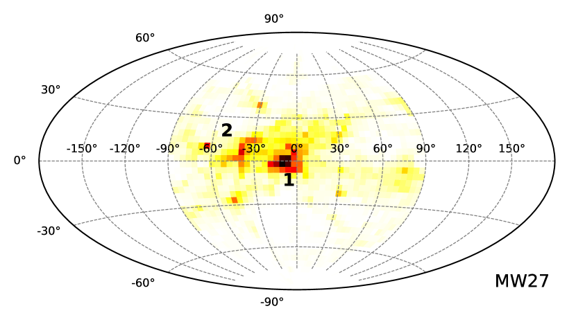
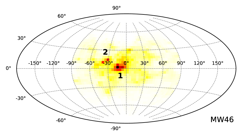
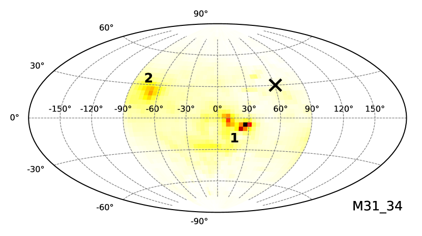
Figure 1: Aitoff projection diagrams of the Milky Way MW27 (top), MW46 (middle) and M31_34 (bottom) 4-galaxy-normal density plots (see also figs. 2 and 4 in Pawlowski et al., 2013). The colormap shows the number of 4-galaxy-normals within a bin, each weighted by $\log\left(\frac{a+b}{c}\right)$ to emphasize planar-like spatial configurations of satellites (see Section 3.1 for details). The total number of 4-galaxy-normals is 1,755,000 for MW27, 16,318,500 for MW46 and 4,637,600 for M31_34, taking into account 100 random realizations of satellite radial distances within the errors for each (see text). The relevant over-density regions in each map are labeled in order of intensity (Peaks 1 and 2 in the main text). Diagrams are in Galactocentric coordinates, centered in the Galactic center. See Tables 4 and 5 for details on the different MW and M31 satellite samples and their data. M31’s spin is marked with an ‘X’. All three diagrams share a common colorbar with values proportional to the normalized bin density.

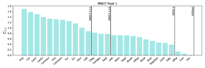
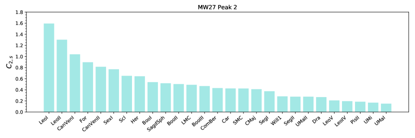
Figure 2: Bar chart showing the weighted-contribution of satellites to 4-galaxy-normals in 15^∘ around the first ($C_{1,s}$, top panel) and second ($C_{2,s}$, bottom panel) most important over-densities found in the Milky Way MW27 density plot (upper panel in Fig. 1). $C_{p,s}$ values are normalized using $C_{N,all}$, the total weighted number of 4-galaxy-normals, included those that are not within 15^∘ of some peak center. The sets of objects that make up the planes of satellites singled out in this work are delimited with vertical lines and labeled correspondingly (see Table 3). Planes quoted in the literature, in particular Pawlowski et al. (2013), are marked with dashed lines.

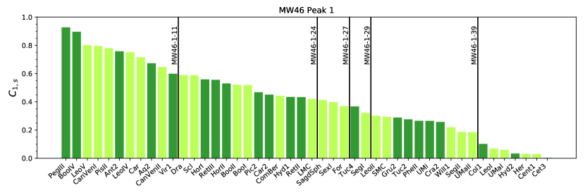
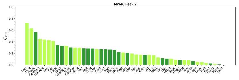
Figure 3: Same as Fig. 2 for the MW46 sample. The contributions from new satellites included in MW46 with respect to MW27 are plotted in a darker color. Note that many of the new satellites considered just fill up the structures already discovered with the MW27 sample (see samples in Table 4).

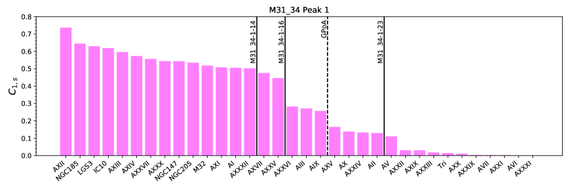
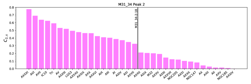
Figure 4: Same as Fig. 2 for M31_34. Both the first (top panel) and second (bottom panel) over-densities of M31’s 4-galaxy-normal density plot have similar strengths (see text and Table 1) which is reflected in a high and comparable contribution from satellites in both bar charts.

4.1 The 4GND plot for the MW27 satellite sample

The upper panel of Fig. 1 shows the Aitoff projection diagram of the 4-galaxy-normal density plot obtained for the MW27 satellite system. This Aitoff diagram can be compared to the contour plot in fig. 2 from P13, to which it is essentially identical.

As reported in P13, the density plot for the MW27 sample shows that 4-galaxy-normals are mainly clustered in the region central to the diagram, revealing a planar structure that is polar to the Galaxy (i.e., the normal vector to the plane is perpendicular to the Galaxy’s spin vector). There is one dominant over-density (Peak 1) located at $(l,b)=(-10.2^{\circ},-0.4^{\circ})$, and a second lower density peak (Peak 2) close to the first at $(l,b)=(-39.7^{\circ},4.5^{\circ})$.

Fig. 2 shows MW27 satellites ordered by $C_{p,s}$ contribution to 4-galaxy-normals within 15^∘ around both density peaks (i.e., $C_{1,s}$, upper panel, and $C_{2,s}$, bottom panel). There are 11 satellites that dominate the contribution (i.e., $C_{p,s}>0.5\times{\rm max}(C_{p,s},s=1,...,27$)), in Peak 1 (i.e., PiscesII, Carina, LeoV, LeoIV, CanesVenaticiI, Draco, CanesVenaticiII, Fornax, Sculptor, SextansI, UrsaMinor), while 4 contribute most in Peak 2 (i.e., LeoI, LeoII, CanesVenaticiI, Fornax). In this case, the contribution is mainly driven by LeoI and LeoII, while the rest of satellites are common with Peak 1 and take low $C_{p,s}$ values, indicating the low relevance of this second structure.

4.2 The 4GND plot for the MW46 satellite sample

In the middle panel of Fig. 1 we plot the Aitoff projection diagram for the 4-galaxy-normal density plot of the MW46 satellite system. This density plot is very similar to that for the MW27 sample (above). Indeed, Peaks 1 and 2 are placed at $(l,b)=(-14.3^{\circ},2.0^{\circ})$ and $(l,b)=(-30.7^{\circ},14.3^{\circ})$, respectively, close to the MW27 main peaks location. In both cases there is a dominant peak and a secondary one, with no other relevant structures. To make the comparison quantitative, in Table 1 we give the values for $C_{\rm MW27,p}$ and $C_{\rm MW46,p}$, with $p$=1,2 for each peak. The peak strengths are somewhat lower for both peaks in the case of MW46 than MW27, as expected given the higher number of satellites and therefore of 4-galaxy-normals.

	$C_{1}\pm\sigma$	$C_{2}\pm\sigma$
MW27	22.92$\pm$0.26	14.31$\pm$0.20
MW46	19.59$\pm$0.19	10.49$\pm$0.13
M31_34	10.53$\pm$0.62	10.52$\pm$1.62
M31_36	11.89$\pm$0.59	9.80$\pm$1.85

Table 1: Peak strengths $C_{p}$ for the main 2 peaks found in the MW27, MW46, M31_34 and M31_36 4GND plots. Peak strength is computed as $C_{p}\equiv\Sigma_{s}C_{p,s}$, and is a percentage, as $C_{p,s}$ is normalized to the total weighted number of 4-galaxy-normals. Errors are calculated from 100 random realizations using the radial distance uncertainties.

Bar charts showing the satellite contribution $C_{p,s}$ to density peaks for the MW46 sample are given in Fig. 3. The contributions from the 21 new satellites that are not in MW27 have been marked with a darker color. Comparing to Fig. 2, we see that i), most satellites belonging to both MW27 and MW46 samples do not appreciably change their contribution to MW peaks, and ii), several satellites among the 21 that are not in MW27 have a relevant contribution to Peak 1 of MW46. An interesting result is that the 25% of satellites that contribute the most to MW27 Peak 1 are included among the 25% of satellites that contribute the most to MW46 Peak 1, complemented with 5 satellites that are not in MW27. Also, out of the 24 satellites that dominate the contribution to Peak 1, 12 are unique to the MW46 increased sample.

As for Peak 2, among the 6 satellites in MW27 contributing the most, all but Fornax are among the 25% main contributors to MW46 Peak 2. And out of the 24 (11) satellites that dominate the contribution to Peak 2, 12 (4) are unique to the MW46 sample.

In summary, the new MW confirmed satellites seem to just add to the positional planar structures already determined with 27 satellites. In the next section this point will be made quantitative through the comparison of the directions of the normal vectors to the different planes.

4.3 Quality analysis

Following our extension to the 4-galaxy-normal method (Section 3.2), for each over-density region we have iteratively computed planes of satellites with an increasing number of members $N_{\rm sat}$, following the order of satellites given in Fig. 2. In this way, for each peak we obtain an ordered collection of planes, one plane for each $N_{\rm sat}$. These collections, and the identities of the $N_{\rm sat}$ satellites belonging to each plane, can be read out of Figs. 2 and 3, for both peaks of the MW27 and MW46 samples, respectively.

The left panel of Fig. 5 shows the characteristics of the planar structures defined by Peak 1 (solid line) and Peak 2 (dashed line) in the MW27 sample. We focus on $c/a$, $b/a$, $D_{\rm cg}$ and the normal direction to the plane. Quantitative results of RMS heights are provided in tables but not shown in our figures as this parameter correlates with $c/a$ presenting the same general trends as $N_{\rm sat}$ increases, and not adding any other relevant information.

The collection of planes obtained for a given over-density region gives rise to a set of points in this plot, with their corresponding error bars, one at each $N_{\rm sat}$ value. They are shown joined with a line, with the corresponding error bands. For Peak 1, errors are shown as a grey shade; for Peak 2 as a cyan shade. These are very narrow (even imperceptible in some cases), showing that the MW27 results are hardly affected by distance uncertainties.

First we see that, for any $N_{\rm sat}$ value, $b/a$ is rather high (and constant), while $c/a$ is low. Therefore configurations are indeed planar-like. Moreover, the lines for both density peaks show rather smooth trends of increasing $c/a$ with increasing $N_{\rm sat}$. In particular, the MW27 Peak 1 line defines a planar structure of satellites with a higher quality (i.e., lower $c/a$ at given $N_{\rm sat}$), than that defined by Peak 2. This is expected, given the higher $C_{p}$ strength of Peak 1 than Peak 2 (see Fig. 1 and Table 1). This suggests that the MW27 satellite sample seems to be a unique highly planar-like organized structure, as we had already learnt from Fig. 2.

In the bottom panels we give the directions of the normal vectors corresponding to the best fitting planes (obtained from the satellites’ most-likely positions) as a function of $N_{\rm sat}$. Shaded regions show the corresponding spherical standard distances $\Delta_{\rm sph}$ (Metz et al., 2007), a measure of the collimation of plane normals for the 1000 realizations. The normal directions to planes from both Peak 1 and 2 in MW27 remain very stable as $N_{\rm sat}$ increases, and their uncertainties due to satellite distance errors are very small.

As for the plane distances to the MW, $D_{\rm cg}$ is below 16 kpc in all plane-fitting iterations in Peak 1, and below 12.5 kpc in the case of Peak 2.

For reference, overplotted colored points in all panels show the values on this diagram for the observed planes of MW satellites mentioned in the literature (classical, VPOS-3, VPOSall; see Table 2), defined from Peak 1 (P13). We note that the points corresponding to the VPOS-3 and VPOSall planes fall over the trend given by the solid line, as expected. On the other hand, and very interestingly, this analysis shows that there is a different combination of $N_{\rm sat}$=11 satellites that results in a much flatter and thinner plane than the classical one (see MW27-1-11 in Table 3). In fact, the plane including $N_{\rm sat}$=14 satellites (MW27-1-14 in Table 3) presents an even higher quality than that with $N_{\rm sat}$=11, as $c/a$ remains roughly constant at a higher $N_{\rm sat}$.

This is possible because this analysis uses the 3-dimensional information of positions, while the classical plane of satellites was found observationally when only the most luminous (i.e. massive) satellites were known to exist. This important result indicates that planes of satellites are not necessarily composed by the most massive satellites of a galactic system (see also Libeskind et al., 2005; Collins et al., 2015) and hence they should not be searched for in this way. Indeed, as we show in Fig. 8, we find that $M_{\rm star}$ is not correlated with $C_{1,s}$ (contribution to the main over-density region, where we find the highest quality planes): the correlation coefficient $r$ is low, in such a way that the probability of getting such value assuming that there is no correlation is higher than 76% (see upper panel in Fig. 8 for MW27 results).

In the right panels of Fig. 5 we plot the results for the MW46 sample. It is very interesting to see that they do not differ that much from those of the MW27 sample, despite the MW46 sample contains 21 satellites that are not members of MW27.

As before, we find planes of satellites with higher qualities than those previously reported with a given $N_{\rm sat}$. For example that with $N_{\rm sat}$ =11, similar to MW27-1-11. More specifically, planes with $N_{\rm sat}$ =24 and 27 present lower $c/a$ values than the VPOS-3 or VPOSall, respectively. These are marked as MW46-1-24 and MW46-1-27 in Figs. 3 and 5 (see Table 3 for the values of their ToI parameters).

In Fig. 5 we can see that the slope of the $c/a$ versus $N_{\rm sat}$ curve grows relatively faster for more than 39 satellites. We hence single out the MW46-1-39 plane with $c/a=0.212\pm 0.002$ as the most populated plane that thin identified so far in the Local Group. A softer discontinuity is also apparent at $N_{\rm sat}=29$, therefore we also emphasize the MW46-1-29 plane as a high quality one (see Table 3). We as well find planes as thin as the VPOS-3 or VPOSall, but more populated (with $N_{\rm tot}$ = 39 and 43 satellites, respectively) and with approximately the same normal direction.

In the two bottom-most panels of Fig. 5 we plot the $(l,b)$ coordinates of the normal vectors to the planes. An interesting result is that the plane with $N_{\rm sat}=24$ has the same direction as the MW27 VPOS-3 (a red circle in the plot), a direction that keeps approximately until $N_{\rm sat}=29$ (i.e., the MW46-1-29 plane), even if the identity of the satellites are not the same, with 13 satellites in MW46-1-29 not in MW27. These panels also indicate that the normals keep their directions within $3^{\circ}$ in $l$ and $4.5^{\circ}$ in $b$, up to $N_{\rm sat}=39$ (i.e. the MW46-1-39 plane). These results quantitatively confirm that many of the new-discovered satellites fill in planes already delineated by members of the MW27 sample, as anticipated in the previous section.

The resemblances between MW27 and MW46 results can be better appreciated by plotting their properties together in terms of $f_{\rm sat}\equiv N_{\rm sat}/N_{\rm tot}$, see Fig. 6. In both cases the quality of Peak 1 is better than that of Peak 2. Moreover, planes identified in the MW27 sample have, at any fixed $f_{\rm sat}$, a slightly better quality than planes in the MW46 collection at the same $f_{\rm sat}$. Therefore, the main planar structure found with the sample of the 46 currently confirmed MW satellites is the same as that previously found with 27 satellites, although they differ in 21 satellite members. These results, with the current data available, corroborate the presence of a vast polar planar structure of satellites around the MW.

We finally note that the true census of MW satellite galaxies is currently far from complete, and thus the robustness of the results presented here requires confirmation in the future. Indeed, some current surveys might bias to find new satellites near the known planar structures. In addition, the advent of new deep surveys reaching increasingly fainter magnitudes and wider sky coverage (like the Rubin Observatory Legacy Survey of Space and Time, LSST), will most probably yield the discovery of a myriad of new faint dwarfs in the virial volume of the MW. The characterization of the spatial distribution of MW satellites will hence need to be progressively updated in order to corroborate our results.

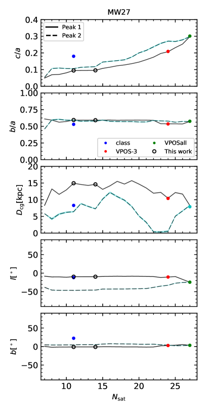
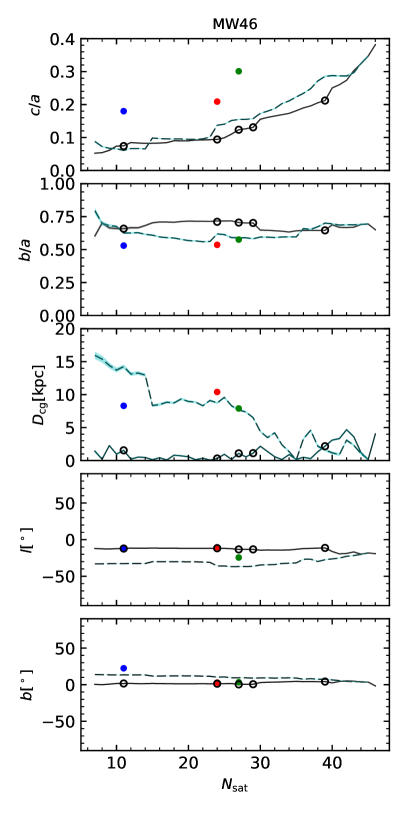
Figure 5: Quality analysis of the main planar structures found in the Milky Way with the 4-galaxy-normal density plot method (see Fig. 1). Left: Pawlowski et al. (2013)’s sample with 27 satellites. Right: the updated MW46 sample with 46 satellites. Lines show $c/a$, $b/a$, $D_{\rm cg}$ and the direction of normal vectors to the best-fitting plane $(l,b)$ as a function of $N_{\rm sat}$. A solid line illustrates results for the Peak 1 planar structure, and a dashed line those for Peak 2. Except in the $l$ or $b$ versus $N_{\rm sat}$ panels, results are the mean values of 1000 realizations at each $N_{\rm sat}$, and shaded regions (gray for Peak 1 and cyan for peak 2) show the standard deviations. Note that these are very small. $(l,b)$ directions have been calculated using the most-likely positions of satellites and shaded regions show the corresponding uncertainties in terms of the spherical standard distance $\Delta_{\rm sph}$ (Metz et al., 2007). As expected, the two curves in each panel converge for the maximum $N_{\rm sat}$ since the samples of satellites considered for each Peak become identical. Colored circles show the results for the reported observed planes of satellites in the MW (classical, VPOS-3, VPOSall). Their specific values including their errors are given in Table 2. The planes of satellites singled out in this work are shown with black open circles, and their corresponding ToI parameters are given in Table 3.

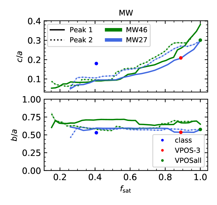
Figure 6: Same as Fig. 5 in terms of the satellite fraction $f_{\rm sat}$. Blue (green) lines are results for the MW27 (MW46) satellite sample.

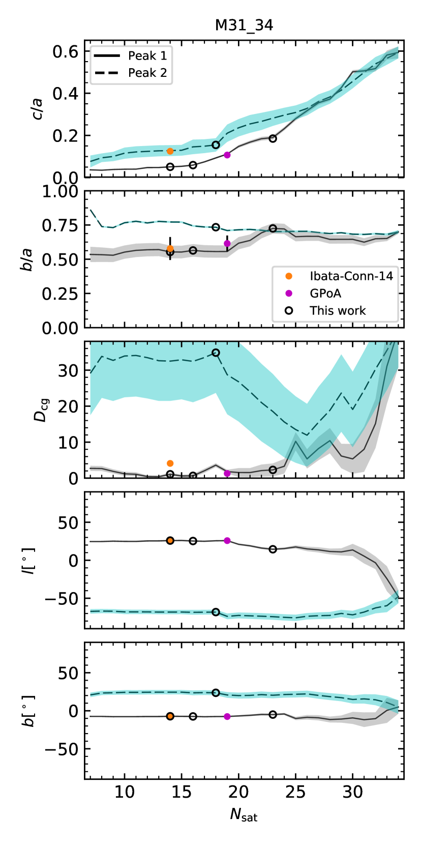
Figure 7: Same as Fig. 5 for the M31_34 satellite sample (reference satellite sample, see Table 5). Colored circles show the results for the reported observed planes of satellites in M31 (‘Ibata-Conn-13’ and GPoA). Their specific values including their errors are given in Table 2. The planes of satellites singled out in this work are shown with black open circles, and their corresponding ToI parameters are given in Table 3.

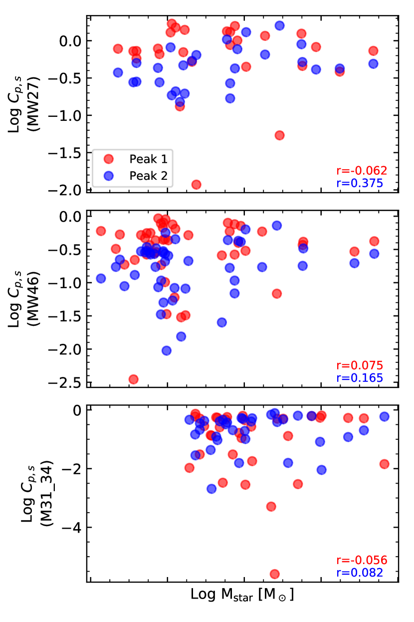
Figure 8: The contribution of satellites to 4-galaxy-normals within 15^∘ of the main density peaks, $C_{p,s}$, versus stellar mass. The Pearson correlation coefficients $r$ are given in each case.

5 Results for Andromeda M31

5.1 The 4GND plot for M31

The lower panel of Fig. 1 reveals, as in the MW, two 4-galaxy-normal density peaks in M31 (reference satellite sample M31_34, see Sec. A). In this case they both show comparable strengths (see Table 1) and are located quite separate from one another. The peak strength values are lower than those of the MW. This is in part due to the higher M31 satellite distance errors (as compared to those of the MW), which blur the peaks in the 4GND plot.

We define Peak 1 as the over-density at $(l,b)=(26.6^{\circ},-6.1^{\circ})$, and Peak 2 as that located at $(l,b)=(-69.1^{\circ},21.7^{\circ})$. The direction of M31’s spin vector, depicted with an ’X’, indicates that the planar configurations defined by both peaks are not perpendicular to the galaxy’s disc, but inclined $\sim 49^{\circ}$ and $\sim 70^{\circ}$, respectively. Interestingly, Peak 1 forms an angle of $\sim 84^{\circ}$ with the MW’s spin vector, meaning its corresponding planes are approximately normal to the MW’s disc (Conn et al., 2013). Furthermore, the projected angular distance on the sphere between Peak 1 and Peak 2 is of $\sim 82^{\circ}$, and the angle between Peak 1 (Peak 2) and the Sun - M31 line is $\sim 88^{\circ}$ ($\sim 5^{\circ}$). Therefore the planar configuration of satellites defined by Peak 1 is observed nearly edge-on from the MW (see table 5 in P13), while that of Peak 2 is approximately perpendicular to it and would be observed mostly face-on.

Fig. 4 shows that approximately half of the satellite sample contributes dominantly to each corresponding peak $p$. Focusing on the identities of satellites, we find that, out of the 16 satellites with highest $C_{1,s}$, 9 are among the satellites with lowest $C_{2,s}$. On the other hand, out of the 16 satellites with highest $C_{2,s}$, 9 are among those with lowest $C_{1,s}$. This is indicating that the two over-densities’ contributing members are not the same. While satellites contributing most to Peak 1 define the GPoA plane from P13 (and also generally coincide with satellites in “plane 1” from Shaya & Tully 2013), Peak 2 defines a separate and independent predominant planar satellite configuration. This structure corresponding to M31_34 Peak 2 has not been analyzed prior to this study and will be described in detail below.

We note that an analysis of the M31_36 sample (i.e., including the satellites AXVI and AXXXIII too) gives quite similar results. As an illustration, in Table 1 we give the values of the corresponding $C_{1}$ and $C_{2}$ peak strengths. The $C_{2}$ values of M31_34 and M31_36 are consistent with each other within their error bars, while the $C_{1}$ strengths are close to be consistent too, with Peak 1 in M31_36 slightly stronger than its M31_34 counterpart. Indeed, for M31_36 we find the same plane structure as in M31_34; i.e., 2 independent peaks pointing in the same normal directions as quoted above for M31_34. In the M31_36 case, AXVI turns out to be the main contributor to Peak 1 (explaining the slight increase of $C_{1}$ strength), while satellite AXXXIII does not contribute to Peak 1, and only mildly to Peak 2.

5.2 Quality analysis

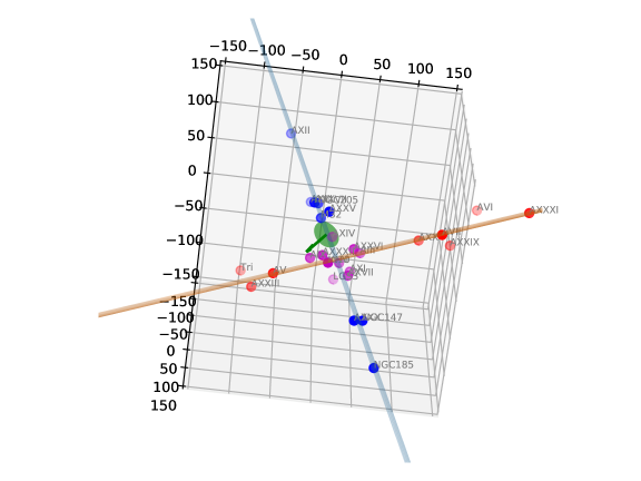
Figure 9: Edge-on view of M31_34-2-18, the highest-quality plane from Peak 2 in M31_34 with $N_{\rm sat}$=18 members (in red), and the GPoA (in blue), showing their relative orientation. M31’s galactic disc and spin vector are depicted in green. Satellites belonging only to the M31_34-2-18 plane are shown as red points, while satellites belonging only to the GPoA are shown as blue points. Satellites shared by both samples are violet.

For each peak, we build up their respective collections of planes of satellites by iteratively applying the best-fitting plane technique to an increasing number of satellites $N_{\rm sat}$, following the order given by Fig. 4. The parameters resulting from the ToI fitting versus $N_{\rm sat}$ are shown in Fig. 7. We see that $c/a$ and $b/a$ take respectively low and high values, confirming that these spatial distributions are actually planes up to $N_{\rm sat}\sim 24-25$. When considering the whole sample of M31_34 satellites, $c/a$ and $b/a$ take a similar value of $\sim 0.6$, indicating instead a non-flattened ellipsoidal spatial distribution (as two approximately perpendicular planes cross).

The corresponding parameter error bands are clearly apparent in the case of M31 as compared to the MW, due to overall larger satellite distance uncertainties. As mentioned previously, while the GPoA is viewed approximately edge-on from the Sun, the planes of satellites from Peak 2 are viewed mostly face-on. Therefore the uncertainties in the Sun - satellite distances affect more (less) to $c/a$ than to $b/a$, in the case of Peak 2 (Peak 1). This fact explains the different magnitude of the error bands of ToI parameters corresponding to different peaks shown in this figure.

Focusing on the $c/a$ panel, one can see that only up to $\sim$half of the total number of satellites contributing respectively to Peak 1 and Peak 2 form a thin planar structure, which rapidly thickens as more members are added to the plane-fitting iteration. Moreover, as said above, satellite identities contributing most to both peaks are overall different, as shown in Fig. 4. Therefore, in contrast to the MW27 and MW46, the M31_34 satellite sample does not form one preferential planar structure but seems to be divided in two.

The normal directions to the planes are stable as $N_{\rm sat}$ increases and reaches $N_{\rm sat}=$19 for Peak 1 and $N_{\rm sat}$=18 for Peak 2, showing that the two satellite planar structures are well defined. Beyond these values, the normals to the corresponding planes are not that well fixed.

As for the distances, planes around Peak 1 pass very close to the M31 center, while planes belonging to Peak 2 do not (see Fig. 7). The values of $D_{\rm cg}$ in this case range between $\sim 12-34$ kpc, within, or close to, the values of $\Delta$RMS for planes associated to Peak 2 (see Table 3). However, the question arises if, given the large radial distance errors and the uncertain potential well of a complex, binary system as is the Local Group, if these distance values are still within reasonable ranges to allow for the possibility of dynamical stability.

The specific values for the M31 Ibata-Conn-14 and GPoA planes are shown with colored circles in Fig. 7 (see Table 2). Our methodology reveals a combination of $N_{\rm sat}$= 14 satellites (marked with a black open circle) that yields a higher quality plane than the ‘Ibata-Conn-14’ plane (see M31_34-1-14 entry in Table 3 and Fig. 4 for satellite identities). This occurs because the ‘Ibata-Conn-14’ plane was defined among only PAndAS survey satellites, while the sample used in P13 and here includes the PAndAS satellites within 300 kpc of M31 (25 out of 27) plus 9 satellites discovered differently (i.e., LGS3, IC10, AXXXII, AVII, AXXIX, AXXXI, AVI, NGC205, M32). Interestingly, the latter turn out to be precisely among the dominant 4-galaxy-normal contributers to both M31_34 Peaks 1 and 2.

In turn, the magenta circles corresponding to the GPoA match the solid line (Peak 1) because the 19 satellites that we find with highest $C_{1,s}$ are precisely the GPoA satellite sample. Note again that the satellite system shows low correlation coefficients $r$ between $M_{\rm star}$ and $C_{1,s}$ or $C_{2,s}$, with a higher than 75% probability of getting such $r$ values assuming that there is no correlation (see Fig. 8).

Moreover, our analysis allows the identification of the highest quality planes in M31 as $N_{\rm sat}$ increases at $c/a$ roughly constant. These planes correspond to the points in Fig. 7 at which the M31_34 Peak 1 and Peak 2 lines start to increase rapidly in the $c/a$ panel, marked in Fig. 7 with black open circles. For Peak 1 we single out a good quality plane at low $c/a$ with $N_{\rm sat}$=16 (M31_34-1-16 in Table 3). We also note the high quality of the plane with $N_{\rm sat}$=23 (M31_34-1-23), with ToI parameter values very similar to those of the VPOS-3 plane of satellites in the MW.

For Peak 2, we highlight the plane with $N_{\rm sat}$=18 members (M31_34-2-18), beyond which the normal vector $\vec{n}(l,b)$ to the best-fitting plane does not conserve its direction. This plane presents comparable properties to the GPoA (magenta circle), to which it is roughly perpendicular. Given that the GPoA has one satellite more and a lower $c/a$ value than the M31_34-2-18 plane (see Tables 2 and 3), strictly speaking the former has a higher quality than the latter. However, the differences are a 5% in $N_{\rm sat}$, and a 10% in the $c/a$ values, if we take into account the error bars. Therefore we can conclude that the qualities of both planes are comparable.

Fig. 9 shows the relative orientation between M31_34-2-18 and the GPoA in a coordinate system oriented such that both planes are seen edge-on. Note that 10 satellites are shared by both samples (i.e., LGS3, IC10, AXIV, AXI, AXXXII, AI, AXVII, AIX, AIII and AXXVI, in violet in the figure).

The quality analysis of the planar structures arising from the M31_36 sample returns similar results to those just presented for M31_34. In most cases, the resulting ToI parameters are consistent with those of M31_34 within 1$\sigma$, or close to being consistent. The only remarkable difference lies in the values of the $b/a$ ratios, larger for the M31_36 planes than for the M31_34 ones with same $N_{\rm sat}$. This occurs because the structure expands as two further away satellites are added to the sample. Fig. 10 illustrates this behaviour in terms of the satellite fraction. Changes of slopes in the $c/a$ versus $N_{\rm sat}$ plot indicate that the high-quality planes to be singled-out have now 1 more satellite for Peak 1, (i.e., M31_36-1-17; M31_36-1-24), or 2 more satellites for Peak 2 (i.e., M31_36-2-20) as compared to those singled out in the M31_34 sample. Their specific ToI values are given in Table 3.

We note that the previously described results for M31 are based on the heliocentric destance moduli given in Table 5, that are those provided in McConnachie (2012)’s data compilation. Using instead distance data from table 2 in Conn et al. (2012) based solely on the ground-based TRGB does not change the results shown in Fig. 7 significantly, and therefore they will be not be made explicit here.

It is of order, nonetheless, to emphasize the sensibility of M31’s Peak 2 planar structure to satellite heliocentric distances, due to its face-on orientation relative to the line-of-sight from the Sun. On one hand, distance uncertainties are indeed large, but these are taken into account and the Peak 2 planar structure is robust in our analysis. However, offsets between the mean distance moduli for the same object coming from different methodologies (HST- or ground-based TRGB and HB; RR Lyrae, etc; see e.g. McConnachie et al., 2005; Conn et al., 2012; Martínez-Vázquez et al., 2017; Weisz et al., 2019) can be in some cases larger than a few times the average thickness of the Peak 2 plane. This is due to calibration issues in each methodology (see discussions in the previous references). Thus, any changes to the distance data used, resulting in a distance dispersion relative to the data assumed here (Table 5) of the order of a few times the $\Delta$RMS of the plane ($\sim 20$ kpc, see Table 3), could end up possibly erasing the M31 Peak 2 planar structure (while keeping that corresponding to Peak 1, whose orientation is close to edge-on with respect to the Sun). The robustness of the Peak 2 plane of satellites will thus have to be confirmed in the future as more accurate and homogeneously-measured M31 satellite distances are available.

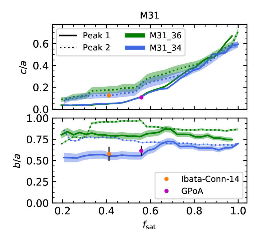
Figure 10: The $c/a$ and $b/a$ ratios in terms of the satellite fraction $f_{\rm sat}$. Blue (green) lines are results for the M31_34 (M31_36) satellite sample.

6 Using full six-dimensional phase-space information

6.1 Co-orbitation within the positionally detected high-quality planes

Proper motion data for MW satellites has revealed one important feature of the plane of satellites observed in the MW: that it presents a high degree of coherent rotation (Metz et al., 2008; Fritz et al., 2018; Pawlowski & Kroupa, 2020). Indeed, the derived orbital angular momentum vectors (i.e., orbital poles, $\vec{J}_{\rm orb}$) of several MW satellites are aligned with the normal to the VPOS-3 within a small angular distance. In particular, Fritz et al. (2018), define co-orbiting satellites within a given plane as those whose orbital poles lie within an angular distance of $36.87^{\circ}$ around the normal to the plane. This corresponds to an area of 10% of the sphere surface (or 20%, when not differentiating objects co-rotating or counter-rotating with the disc of the central galaxy).

We study if the MW satellites included in the high-quality planes detected with the 4GND plot method are co-orbiting within them. To this end we measure the angular distance between the normal vector to a given singled-out plane, $\vec{n}$, and each individual satellite orbital pole $\vec{J}_{\rm orb}$. We consider 36 satellites from the MW46 sample, for which kinematic data is currently available. In particular, the orbital poles for the LMC and SMC are taken from Gaia Collaboration et al. (2018), while those of the rest of satellites are taken from Fritz et al. (2018), Fritz et al. (2019) and Torrealba et al. (2019). We refer the reader to these papers for details.

The projection on the sky of these orbital poles is shown in green in Fig. 12, with the actual direct measurements depicted as circles with labels, while 2000 Monte Carlo simulations of the poles including measurement errors, are shown as tiny points. In this Aitoff diagram, orbital poles are shown as all co-rotating with the disc of the MW. Objects that are actually counter-rotating are distinguished by a lighter green color. Note however that, for those MW satellites whose orbits are close to perpendicular to the Galactic disc, the fact that they are measured as rotating or counter-rotating is not well-determined, but within the errors.

Fig. 11 shows the fraction of the total number of satellites with $\vec{J}_{\rm orb}$ enclosed by a certain angle $DA$ from the reference axis $\vec{n}$ (note that in this figure we do not differentiate between co-rotation or counter-rotation with the disc of the central galaxy, therefore the angular distance $DA$ can be a maximum of 90^∘). Solid and dashed black lines give the clustering results around the directions of MW46 Peak 1 and 2, respectively. These lines show the mean value of 1000 Monte Carlo random realizations of orbital pole projections, while a shaded area shows the $\pm 1\sigma$ dispersion range. A yellow vertical line is drawn at $DA=36.87^{\circ}$, while a dotted line shows the expected result for an isotropical distribution of orbital poles. It is clear that the normal direction to Peak 1 defines a plane with a higher degree of satellite co-orbitation, than that of Peak 2. In particular, there is a $44\pm 5\%$ of co-orbiting satellites around Peak 1 and a $31\pm 5\%$ around Peak 2. Note that if assuming directly the measured orbital poles (circles in Fig. 12), these fractions increase to $50\%$ and $39\%$, respectively.

When using instead as reference axis the normal directions to specific singled-out planes from MW46 we obtain a very similar result to that with the Peak 1 axis. As an example, we show with a green line the clustering obtained with respect to the normal vector to MW46-1-39 (the normal directions to Peak 1 and MW46-1-39 are separated only by $2.8^{\circ}$).

These results indicate that approximately half of the satellites belonging to positionally-detected, high-quality planes share coherent motion, while the other half could mostly be lost to the plane in a short time after observation. Results qualitatively consistent with these ones have also been found in cosmological simulations (see Paper II, Gillet et al., 2015; Buck et al., 2016; Shao et al., 2019).

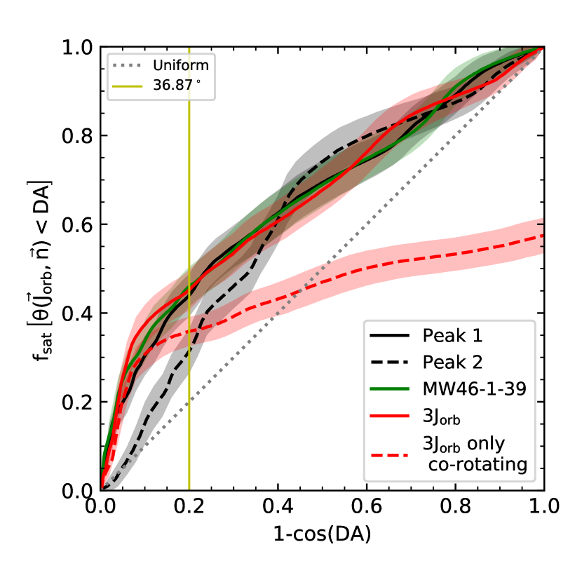
Figure 11: Fraction of MW46 satellites with orbital poles enclosed in a given angle $DA$ measured from different reference axes: 4GND plot Peaks 1 and 2 (black solid and dashed line, respectively); the normal to the MW46-1-39 plane (green), and the main peak of the 3J_orb-barycenter density plot (red). We do not differentiate between co-rotating or counter-rotating orbital poles with the disc of the galaxy. Only for the last axis do we show as well the results of only co-rotating MW satellites (red dashed). Solid lines show the median values while shaded areas the $\pm\sigma$ range. Uncertainties have been computed from assuming 1000 random realizations of the orbital poles including measurement errors. The dotted line shows the result for a uniform distribution, and a yellow vertical line marks an angle of 36.87^∘. In Fritz et al. (2018), MW satellites with orbital poles enclosed within this angle from the VPOS-3 are considered to be co-orbiting within the plane.

Concerning M31, it is of interest whether the M31_34-2-18 plane could be dynamically stable, this is, if the member satellites co-orbit within the planar structure they define in space. While in the lack of proper motion measurements for M31 satellites, line-of-sight velocities of the satellites involved in the M31_34-2-18 plane (taken from McConnachie, 2012; Collins et al., 2013; Martin et al., 2014), which we observe face-on from the MW, give a perpendicular velocity dispersion of $\sigma=90.20$ km/s. According to Fernando et al. (2017), such a plane will be erased in a short timescale and is just a fortuitous alignment of satellites, as they find that planes with a perpendicular velocity dispersion above $\sim 50$ km/s disperse to contain half their initial number of satellites in 2 Gyrs time.

This result should be taken with caution, and confirmed when 3D-velocities are available, as numerical experiments have shown that line-of-sight velocities are not well representative of the former (Buck et al., 2016). We note even so, that, as this plane is observed face-on from the MW, it is not expected that the consideration of the tangential velocities may change much the perpendicular velocity dispersion estimated here. What may be more relevant to this face-on plane, however, are the very uncertain radial distance measurements to M31 satellites, as discussed earlier. Thus, until this position data achieves higher accuracy and consistency between methodologies, the outcomes of a dynamical assessment of this spatial structure will remain less convincing.

6.2 Identifying the axes of maximum satellite co-orbitation

Neither the 4GND plot method, or its extension, are designed to identify planes of kinematically-coherent satellites able to persist in time, as they focus only on the position of satellites. In Paper III (Santos-Santos, in preparation) the 3J_orb-barycenter method is introduced, which leads to the identification of axes around which a maximum number of satellites co-orbit out of a sample of $N_{\rm tot}$ of them. Combining the results at different times, high quality, persistent planes of satellites are identified in simulations of disc galaxies.

Briefly, this method consists in finding clustering in the space of orbital angular momentum vector projections, following a protocol similar to that of the 4GND plot method (see also Garaldi et al., 2018). Given the orbital poles of a satellite set, the barycenters of all the spherical triangles that can be formed out of the $N_{\rm tot}$ poles are calculated. This gives $N_{\rm 3Jorb}$ points on the sphere (the combinations of $N_{\rm tot}$ over 3). Such a method multiplies the statistics as an asset to search for clustering within an otherwise small set of satellite orbital poles. A smoothing similar to that described in Section 3, leads to the so-called 3J_orb-barycenter density plot, whose maxima represent directions around which the orbital poles cluster. The method allows us to determine where these maxima are placed on the sphere; that is, the normal directions to planes that are kinematically-coherent by construction.

This method has been applied to the subsample of MW46 satellites for which kinematic data are available, described in the previous subsection. The corresponding 3J_orb-barycenter density plot is drawn in Fig. 12, in the background of the Aitoff diagram. In particular, 100 realizations have been stacked, where we consider 100 orbital pole directions taken at random from the 2000 Monte Carlo simulations including the measurement errors. One unique remarkable overdensity stands out, with its peak at $(l,b)=(-2.1^{\circ},6.1^{\circ})$ (the densest bin is circled in black). This axis is only 4.6^∘ apart from the normal direction to the VPOS-3, marked with a blue ’X’ (see Table 2), and therefore also very close to the normals of all planes corresponding to Peak 1 found with the position-only 4GND plot method (see Table 3).

We use now the new axis found with the 3J_orb-barycenter method to compute the fraction of co-orbiting MW satellites. This is shown in red in Fig. 11. There is a slightly higher fraction of co-orbiting satellites at small $DA$ than in the cases when assuming the normal directions to the positionally-detected planes (black lines), but approximately the same mean and dispersion is found at $DA=36.87^{\circ}$ than for Peak 1. Translating to absolute numbers, we find $16\pm 2$ co-orbiting satellites out of the considered sample with $N_{\rm tot}=36$. If focusing on the actual measured values, $18$ satellites co-orbit (see objects within big black circle in Fig. 12, i.e., PiscesII, Draco, Hydrus1, Carina, CanesVenaticiII, LMC, SMC, Crater2, UrsaMinor, CanesVenaticiI, Aquarius2, Carina3, Sculptor, LeoV, Fornax, ReticulumII, HorologiumI, PhoenixII). Interestingly, if only considering co-rotation with the Galactic disc, the mean fraction of co-orbiting satellites is $36\%$, which corresponds to $13$ satellites ($14$ if assuming the actual measurements), which shows that counter-rotating satellites in this structure are a minority (only $4$, i.e., CanesVenaticiII, Aquarius2, Sculptor, LeoV).

For the sake of comparison, the MW27 sample has also been kinematically analyzed through the 3J_orb-barycenter method. In this case, 25 of its members have kinematic information. Again, a unique remarkable 3J_orb axis has been identified, which happens to be very close to that of the MW46 satellites $(l,b)=(-1.0^{\circ},5.1^{\circ})$. The fraction of the 25 satellites with poles at angular distance $<DA$ around this axis is given in Fig. 13, where we also plot the corresponding result for the MW46 satellites (red solid line in Fig.11). They show indistinguishable clustering properties within the error bars, with a slighly larger mean in the case of MW46. Therefore, with the current kinematic data and within the error bands, the newly identified satellites relative to MW27 follow the kinematic structure already present with MW27 satellites.

These results show how this new method directly identifies a rotation axis whose corresponding normal plane contains the maximum possible number of satellites co-orbiting within it. In paper III the method is applied to two zoom-in hydro-simulations of disc galaxies, and a persistent plane, with the same satellite members along cosmic evolution, is identified in each case.

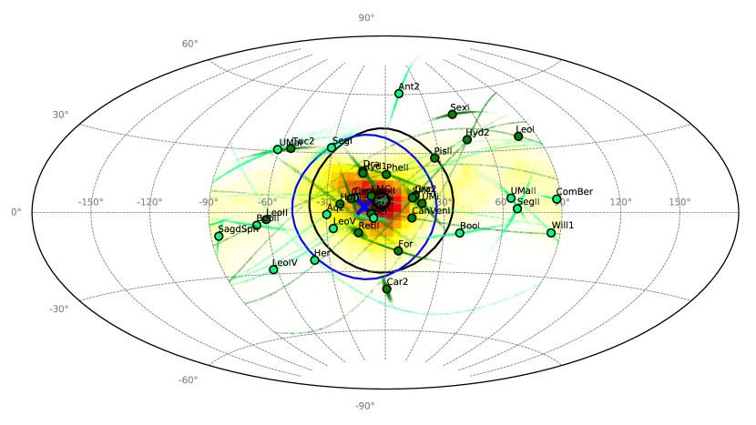
Figure 12: Aitoff diagram showing the orbital poles of MW satellites (data from Gaia Collaboration et al., 2018; Fritz et al., 2018, 2019; Torrealba et al., 2019). Actual measurement values are shown as circles and 2000 Monte Carlo simulations including uncertainties are shown as clouds of small points. These are Galactocentric coordinates, centered in the Galactic center. All orbital poles are plotted within [-90^∘,+90^∘] in longitude, as if they all co-rotate with the MW’s Galactic disc. A lighter green color marks satellites that are actually counter-rotating. In the background is the density plot resultant of applying the ’3Jorb-barycenter method’ (See Section 6.2). It has been computed by stacking the result of 100 random realizations of the orbital poles, taking into account measurement errors. The densest bin, and therefore the direction of the main co-orbitation axis found with this method, is circled in black. A blue cross marks the normal direction to the VPOS-3 plane. Additionally, we show circles withstanding an angle of 36.87^∘ from the previous axes (see text).

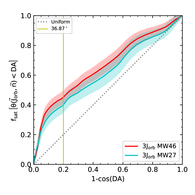
Figure 13: Same as Fig.11, comparing the results of the 3J_orb-barycenter method applied to the samples of MW satellites with kinematical information drawn from MW27 and MW46 (see Table 4).

7 Summary and conclusions

Recent studies on planes of satellites have resorted to evermore refined methods to define and characterize them. In this work, we have further developed one such method, the ’4-galaxy-normal density plots’ method (P13) with an extension designed to identify, systematically catalog and study in detail the quality of the predominant planar configurations revealed by over-densities in the 4-galaxy-normal density plots. The method has been applied to the currently considered confirmed satellite galaxies of the MW and M31 systems (no nearby dwarfs, globular clusters or streams have been considered), providing the most detailed and updated characterization of their satellite planar-like spatial distributions. These serve as a reference with which to compare results from numerical hydrodynamical simulations of disc galaxy systems (see, e.g., Paper II).

We count the weighted number of times each satellite $s$ contributes to 4-galaxy-normals within 15^∘ of a specific over-density $p$ identified in a density plot ($C_{p,s}$). For each relevant over-density, we define its peak strength as $C_{p}=\sum_{s}C_{p,s}$, normalized to the total number of 4-galaxy-normals. We order satellites by decreasing $C_{p,s}$ and iteratively fit planes to subsamples of satellites following this order. In this way, rather than a plane per over-density, we yield a catalog or collection of planes of satellites with an increasing number of members $N_{\rm sat}$, whose normals cluster around the density peak. This method selects the subsamples of $N_{\rm sat}$ satellites with lowest $c/a$ provided that they are embedded in a larger, populated, predominant planar structure. Indeed, in the case of planes with high $N_{\rm sat}$/$N_{\rm tot}$, the method selects the subsample of satellites that yields the thinnest plane out of all possible combinations of $N_{\rm sat}$ satellites. On the other hand, for low $N_{\rm sat}$/$N_{\rm tot}$ planes, it avoids choosing subsamples of satellites that form very narrow planes but are just chance alignments, i.e., not embedded in larger planar structures.

The quality of planes is quantified through the number of member satellites $N_{\rm sat}$ and the degree of flattening. The latter is measured through the short-to-long axis ratio of the Tensor of Inertia (ToI, Metz et al., 2007) concentration ellipsoid, $c/a$ provided there is a high intermediate-to-long axis ratio, $b/a$, which confirms a planar-like spatial distribution of satellites (the RMS thickness normal to the plane is correlated to $c/a$ and it does not add further information). Quality comparisons between planes are done either considering constant $N_{\rm sat}$ (where a lower $c/a$ means higher quality) or constant $c/a$ (where more populated planes have higher quality). In this way, we are able to single out new high-quality planes.

This method has been applied to the most up-to-date positional data of MW and M31 confirmed satellites (see Tables 4 and 5, and references therein). In the case of the MW we consider a total of $N_{\rm tot}=$46 satellite galaxies (sample MW46). Also, for the sake of comparison with P13’s results and with numerical simulations, we have also studied the same satellite sample as in P13, consisting of $N_{\rm tot}=$ 27 satellites. In the case of M31 we consider the 34 satellites within 300 kpc from M31. Moreover, contemplating the possibility of M31’s larger total virial mass and radius relative to the MW, we have extended the limiting satellite distance to 350 kpc, hence including satellites AXVI and AXXXIII in a complementary analysis.

Two predominant, collimated over-density regions show up in the 4-galaxy-normal density plots of both the MW and M31. They reveal that both their satellite systems are highly structured in planar-like configurations. However, they show very different patterns: while satellites in the MW form basically one main polar structure (either in the $N_{\rm tot}$ = 27 or 46 samples), M31 satellites are spatially distributed along two distinct collections of planes, inclined with respect to the M31 disc and roughly perpendicular to each other.

We find planes of satellites with higher qualities than those previously reported with a given $N_{\rm sat}$. More specifically, we find a combination of 11 MW satellites that spatially describe a plane with much higher quality than that defined by the 11 classical (i.e., the most massive) satellites. Similarly, we find combinations of $N_{\rm sat}$ =24 and 27 satellites with lower $c/a$ values than the VPOS-3 or VPOSall, respectively. We have also found planes as thin as the VPOS-3 or VPOSall, but more populated (with $N_{\rm sat}$ = 30 and 34 satellites, respectively) and with approximately the same normal direction. We single out the plane with $N_{\rm sat}$ = 39 (MW46-1-39 in Table 3) with $c/a=0.212\pm 0.002$, as the most populated plane that thin identified so far in the Local Group; this is our most noticeable result for the Milky Way. Another remarkable result is that, when expressed in terms of the satellite fraction $f_{\rm sat}\equiv N_{\rm sat}/N_{\rm tot}$, results for the MW satellite sample with 46 satellites follow planar structures found for the sample with 27 satellites (VPOS), although they differ in 21 satellite members. This proves how the MW’s polar plane of satellites is a robust structure that endures as the census of MW satellites increases in number. However, some words of caution are in order, as these results will need to be continuously revised as new ultrafaint galaxies are discovered with upcoming deep surveys.

An analysis through the clustering of the satellite orbital poles indicates that at least $\sim 45\%$ of satellites co-orbit within these new-identified planes, with a fraction of $\sim 50\%$ consistent within the errors (this is not differentiating between co- and counter-rotating with the MW disc). Furthemore, in order to study the kinematical-coherence of MW satellites in an independent way, we briefly introduce the ’3J_orb-barycenter’ method. This method aims at identifying orbitation axes whose normal planes contain the maximum possible number of kinematically-coherent satellites out of $N_{\rm tot}$ of them (the so-called ’3J_orb’ axes). We apply this method to the samples of satellites with kinematical information drawn from MW27 and MW46, and find that in each case, a unique orbitation 3J_orb axis stands out, with the particularities that they both point to approximately the same direction and that this direction is only $\sim 3^{\circ}$ away from the normal vector to the MW46-1-39 plane. Clustering of orbital poles around these two 3J_orb axes of either MW27 or MW46 satellites yields results that are consistent within the error bands, and are also consistent with clustering around the MW46 Peak 1 direction, or the normal vector to the MW46-1-39 plane: $45\pm 5$% satellites co-orbit around any of these axes.

As for M31, for the first time, the second-most predominant planar structure (Peak 2) found in M31 has been studied in detail. This peak points to a satellite planar configuration whose normal direction aligns with the line-of-sight between the Sun and M31, and therefore is viewed nearly face-on (we recall that the planar configuration defined by M31 Peak 1 –containing the well-known GPoA with $N_{\rm sat}$=19– is viewed nearly edge-on). Our analysis reveals a rich plane structure, with quality behaviour in terms of $c/a$ versus $N_{\rm sat}$ similar to that found around Peak 1, despite being more affected by the radial Sun - satellite distance uncertainties due to its orientation. As quantitatively shown by similar peak strength $C_{p}$ values, this is an independent planar structure to that defined by Peak 1. Indeed, different subsamples of satellites contribute dominantly to each structure, while there is a $\sim$50% of shared satellites that contribute less.

We present a combination of 14 M31 satellites from Peak 1 with much lower $c/a$ values than those of the plane noted by Ibata et al. (2013) and Conn et al. (2013) (Ibata-Conn-14 plane) with the PAndAS survey. Also, $c/a$ starts increasing more sharply for $N_{\rm sat}>16$ satellites around Peak 1, and for $N_{\rm sat}>18$ around Peak 2. Therefore we single out the planes of satellites with precisely these $N_{\rm sat}$ values as they present exceptional quality. As evidence, the planes’ normals stay stable up to $N_{\rm sat}\sim 19$ for Peak 1, and $N_{\rm sat}\sim 18$ for Peak 2, and then they change. Interestingly, the plane from Peak 1 with $N_{\rm sat}$=16 is more populated and thinner than the Ibata-Conn-14 plane. Moreover, the plane with $N_{\rm sat}$=18 from Peak 2 presents very similar properties to the GPoA while consisting of an overall different satellite sample: $c/a$ is $0.15\pm 0.03$. A first approach to its kinematics through the available line-of-sight velocities suggests a high perpendicular velocity dispersion that would soon disperse the plane. This should be confirmed however with proper motions and 3D velocity data in the future.

Adding to the analysis the two further away M31 satellites placed beyond 300 kpc does not change these conclusions. Quantitatively, the $b/a$ ratios increase (as the size of the system considered is larger) but the rest of the ToI parameters of Peaks 1 and 2 planes remain essentially the same.

We however have to caution the reader about the sensibility of the M31 Peak 2 planar structure to satellite distance determinations. Due to its almost face-on orientation relative to the line-of-sight from the Sun, any changes in the distance moduli data used, resulting in a distance dispersion relative to the data assumed in this work (Table 5) of the order of a few times the $\Delta$RMS of this plane, could possibly erase the positionally-detected Peak 2 plane. This can be an issue, as distance moduli for a same object obtained with different methodologies can be very different (because the calibrations they are based on are different and not well fixed; see discussions in Martínez-Vázquez et al., 2017; Weisz et al., 2019).

Finally, the richer plane structure in the MW and M31 we report in this work was found because we allow the mass of satellites to play no role in our search. Indeed, through correlation tests we find that mass is not a satellite property that determines its 4-galaxy-normal contribution to the main over-density regions (i.e., its membership or not to the respective high-quality planes), either in the MW or M31 cases. This idea is supported by the fact that young globular clusters and some streams align as well with the MW’s VPOS (see Pawlowski et al., 2012; Riley & Strigari, 2020).

We conclude that the 4GND plot method and its quality analysis extension allow for an accurate and detailed characterization of the predominant planar spatial configurations of satellites underlying a given (observed or simulated) galactic system. Applied to currently available MW data, we find and characterize a unique dominant planar structure, and highlight a remarkably thin plane of satellites involving 39 over 46 satellites. Of these, $\sim 45$% are in coherent orbitation. Applied to M31 data, two equivalent, orthogonal planar structures have been found, each involving $\sim 19$ over 36 satellites.

Table 2: ToI fitting properties of the observed planes of satellites in the MW (classical, VPOSall, VPOS-3) and M31 (Ibata-Conn-14, GPoA): Galactic coordinates of the normal to the plane; uncertainty in the normal direction; distance to the MW/M31; root-mean-square height of the plane; short-to-long ellipsoid axis ratio; intermediate-to-long ellipsoid axis ratio; number of satellites included in the plane. Information for the classical plane of MW satellites has been taken from Metz et al. (2007) and Pawlowski (2016). The information for all rest of planes has been extracted from Pawlowski et al. (2013) (see their table 3), where distance uncertainties are considered by sampling the distances 1000 times with a Gaussian distribution around their most-likely distance.

	MW			M31
Name	classical	VPOSall	VPOS-3	Ibata-Conn-14	GPoA
$\vec{n}(l,b)$ [∘]	(-22.7, 12.7)	(-24.4, 3.3)	(-10.5, 2.8)	(26.2, -7.8)	(25.8, -7.6)
$\Delta_{\rm sph}n$ [∘]	–	1.12	0.43	1.00	0.79
$D_{\rm MW}$ [kpc]	8.3	7.9 $\pm$ 0.3	10.4 $\pm$ 0.2	–	30.1 $\pm$ 8.8
$D_{\rm M31}$ [kpc]	–	637.3 $\pm$ 13.0	509.9 $\pm$ 10.2	4.1 $\pm$ 0.7	1.3 $\pm$ 0.6
$\Delta$RMS height [kpc]	19.6	29.3 $\pm$ 0.4	19.9 $\pm$ 0.3	14.2 $\pm$ 0.2	13.6 $\pm$ 0.2
$c/a$	0.18	0.301 $\pm$ 0.004	0.209 $\pm$ 0.002	0.125 $\pm$ 0.014	0.107 $\pm$ 0.005
$b/a$	0.53	0.576 $\pm$ 0.007	0.536 $\pm$ 0.006	0.578 $\pm$ 0.084	0.615 $\pm$ 0.058
$N_{\rm sat}$	11	27	24	14	19

Table 3: Same as Table 2 for the high quality planes singled out in this work.

	[Host-Peak-$N_{\rm sat}$]
Name	MW27-1-11	MW27-1-14	MW46-1-11	MW46-1-24	MW46-1-27	MW46-1-29	MW46-1-39
$\vec{n}(l,b)$ [∘]	(-9.6, -1.1)	(-9.7, -1.1)	(-12.14, 1.61)	( -11.73, 1.33)	( -13.32, 0.39)	(-13.27, 0.60)	(-11.29, 4.24)
$\Delta_{\rm sph}n$ [∘]	0.15	0.15	0.18	0.16	0.16	0.17	0.26
$D_{\rm MW}$ [kpc]	15.0$\pm$0.1	14.6$\pm$1.0	1.6$\pm$0.1	0.3$\pm$0.1	1.1$\pm$0.1	1.1$\pm$0.1	2.2$\pm$0.1
$D_{\rm M31}$ [kpc]	464.5$\pm$6.3	465.2$\pm$6.3	518.2$\pm$6.9	511.7$\pm$6.8	520.3$\pm$6.9	520.9$\pm$6.9	518.6$\pm$7.0
$\Delta$RMS height [kpc]	11.6$\pm$0.1	10.3$\pm$0.1	9.8$\pm$0.1	9.1$\pm$0.1	11.8$\pm$0.1	12.1$\pm$0.1	19.1$\pm$0.2
$c/a$	0.095$\pm$0.001	0.096$\pm$0.001	0.074$\pm$0.001	0.094$\pm$0.001	0.124$\pm$0.001	0.131$\pm$0.01	0.212$\pm$0.002
$b/a$	0.595$\pm$0.004	0.592$\pm$0.004	0.659$\pm$0.011	0.711$\pm$0.005	0.705$\pm$0.005	0.702$\pm$0.005	0.646$\pm$0.005
$N_{\rm sat}$	11	14	11	24	27	29	39
Name	M31_34-1-14	M31_34-1-16	M31_34-1-23	M31_34-2-18	M31$\_$36-1-17	M31$\_$36-1-24	M31$\_$36-2-20
$\vec{n}(l,b)$ [∘]	(25.9, -7.2)	(25.3, -7.4)	(14.4, -5.0)	(-68.2, 23.6)	(25.3, -7.5)	(18.9, -5.8)	(-60.5, 21.6)
$\Delta_{\rm sph}n$ [∘]	0.45	0.51	1.40	3.16	0.30	0.82	3.14
$D_{\rm MW}$ [kpc]	36.2$\pm$4.9	40.9$\pm$5.8	185.7$\pm$15.0	741.6$\pm$6.5	42.7$\pm$3.3	131.8$\pm$8.7	748.0$\pm$5.1
$D_{\rm M31}$ [kpc]	1.1$\pm$0.4	0.6$\pm$0.5	2.3$\pm$1.8	34.9$\pm$11.2	0.7$\pm$0.5	1.8$\pm$1.2	38.6$\pm$12
$\Delta$RMS height [kpc]	7.0$\pm$0.2	7.7$\pm$0.2	21.4$\pm$1.0	21.0$\pm$4.2	7.2$\pm$0.2	22.5$\pm$0.7	28.7$\pm$4.8
$c/a$	0.051$\pm$ 0.002	0.059$\pm$0.002	0.189$\pm$0.009	0.155$\pm$0.032	0.059$\pm$0.002	0.207$\pm$0.007	0.227$\pm$0.038
$b/a$	0.553$\pm$0.046	0.564$\pm$0.046	0.725$\pm$0.038	0.734$\pm$0.006	0.797$\pm$0.004	0.871$\pm$0.036	0.973$\pm$0.011
$N_{\rm sat}$	14	16	23	18	17	24	20

Data availability

The observational data for Milky Way and M31 satellite galaxies analyzed in this article comes from the following references: McConnachie (2012); Conn et al. (2012); Simon (2019), http://www.astro.uvic.ca/~alan/Nearby_Dwarf_Database_files/NearbyGalaxies.dat. Note that the latter is a compilation of data, and the original sources of the data are indicated therein. The data used has been summarized for reference in this article in Tables 4 and 5.

Appendix A MW and M31 data used in this paper

Table 4: Data for MW confirmed satellite galaxies used in this paper, separated in the MW27 and MW46 sample. The MW46 sample includes all MW27 satellite galaxies, except for CanisMajor and BootesIII, which are marked with an asterisk. Columns show the position in right ascension and declination, the distance modulus, the linear heliocentric distance we derive from the distance modulus, and the stellar mass (estimated assuming Woo et al. (2008)’s M/L ratios according to galaxy morphological type). For references we refer the reader to McConnachie (2012)’s data compilation.

GalaxyName	RA/deg	Dec/deg	$(m-M)\pm$err	D⊙/kpc${}^{\rm+err}_{\rm-err}$	Mstar/M⊙
MW27
BootesI	210.03	14.50	19.11 $\pm$ 0.08	66.37 ${}^{2.49}_{2.40}$	3.50E+04
BootesII	209.50	12.85	18.10 $\pm$ 0.06	41.69 ${}^{1.17}_{1.14}$	2.05E+03
BootesIII*	209.30	26.80	18.35 $\pm$ 0.10	46.77 ${}^{2.20}_{2.11}$	2.73E+04
CanesVenatici1	202.01	33.56	21.69 $\pm$ 0.10	217.77 ${}^{10.26}_{9.80}$	3.73E+05
CanesVenaticiII	194.29	34.32	21.02 $\pm$ 0.06	159.96 ${}^{4.48}_{4.36}$	1.60E+04
CanisMajor*	108.15	-27.67	14.29 $\pm$ 0.30	7.21 ${}^{1.07}_{0.93}$	7.80E+07
Carina	100.40	-50.97	20.11 $\pm$ 0.13	105.20 ${}^{6.49}_{6.11}$	8.09E+05
ComaBerenices	186.75	23.90	18.20 $\pm$ 0.20	43.65 ${}^{4.21}_{3.84}$	7.73E+03
Draco	260.05	57.92	19.40 $\pm$ 0.17	75.86 ${}^{6.18}_{5.71}$	4.17E+05
Fornax	40.00	-34.45	20.84 $\pm$ 0.18	147.23 ${}^{12.72}_{11.71}$	3.31E+07
Hercules	247.76	12.79	20.60 $\pm$ 0.20	131.83 ${}^{12.72}_{11.60}$	2.94E+04
LeoI	152.12	12.31	22.02 $\pm$ 0.13	253.51 ${}^{15.64}_{14.73}$	7.05E+06
LeoII	168.37	22.15	21.84 $\pm$ 0.13	233.35 ${}^{14.40}_{13.56}$	1.08E+06
LeoIV	173.24	0.53	20.94 $\pm$ 0.09	154.17 ${}^{6.52}_{6.26}$	1.36E+04
LeoV	172.79	2.22	21.25 $\pm$ 0.12	177.83 ${}^{10.10}_{9.56}$	7.87E+03
LMC	80.89	-69.76	18.52 $\pm$ 0.09	50.58 ${}^{2.14}_{2.05}$	1.06E+09
PiscesII	344.63	5.95	21.31 $\pm$ 0.17	182.81 ${}^{14.89}_{13.77}$	6.73E+03
SagittariusdSph	283.83	-30.55	17.10 $\pm$ 0.15	26.30 ${}^{1.88}_{1.76}$	3.44E+07
Sculptor	15.04	-33.71	19.67 $\pm$ 0.14	85.90 ${}^{5.72}_{5.36}$	2.91E+06
SegueI	151.77	16.08	16.80 $\pm$ 0.20	22.91 ${}^{2.21}_{2.02}$	4.53E+02
SegueII	34.82	20.18	17.70 $\pm$ 0.10	34.67 ${}^{1.63}_{1.56}$	7.59E+02
SextansI	153.26	-1.61	19.67 $\pm$ 0.10	85.90 ${}^{4.05}_{3.87}$	6.98E+05
SMC	13.19	-72.83	19.03 $\pm$ 0.12	63.97 ${}^{3.63}_{3.44}$	3.23E+08
UrsaMajorI	158.72	51.92	19.93 $\pm$ 0.10	96.83 ${}^{4.56}_{4.36}$	1.53E+04
UrsaMajorII	132.88	63.13	17.50 $\pm$ 0.30	31.62 ${}^{4.69}_{4.08}$	6.86E+03
UrsaMinor	227.29	67.22	19.40 $\pm$ 0.10	75.86 ${}^{3.58}_{3.41}$	5.60E+05
Willman1	162.34	51.05	17.90 $\pm$ 0.40	38.02 ${}^{7.69}_{6.40}$	1.41E+03
MW46
Antlia2	143.89	-36.77	20.60 $\pm$ 0.11	131.83 ${}^{6.85}_{6.51}$	5.60E+05
Aquarius2	338.48	-9.33	20.16 $\pm$ 0.07	107.65 ${}^{3.53}_{3.41}$	7.59E+03
BootesIV	233.69	43.73	21.60 $\pm$ 0.20	208.93 ${}^{20.16}_{18.38}$	8.87E+03
Carina2	114.11	-58.00	17.79 $\pm$ 0.05	36.14 ${}^{0.84}_{0.82}$	8.63E+03
Centaurus1	189.58	-40.90	20.33 $\pm$ 0.10	116.41 ${}^{5.49}_{5.24}$	2.27E+04
Cetus3	31.33	-4.27	22.00 $\pm$ 0.20	251.19 ${}^{24.23}_{11.31}$	1.31E+03
Columba1	82.86	-28.03	21.30 $\pm$ 0.22	181.97 ${}^{19.40}_{17.53}$	8.63E+03
Crater2	177.31	-18.41	20.35 $\pm$ 0.02	117.49 ${}^{1.09}_{1.08}$	2.61E+05
Grus2	331.02	-46.44	18.62 $\pm$ 0.21	52.97 ${}^{5.38}_{4.88}$	5.06E+03
HorologiumI	43.88	-54.12	19.50 $\pm$ 0.20	79.43 ${}^{7.66}_{6.99}$	3.60E+03
HorologiumII	49.13	-50.02	19.46 $\pm$ 0.20	77.98 ${}^{7.52}_{6.86}$	5.76E+02
Hydra2	185.43	-31.99	20.64 $\pm$ 0.16	134.28 ${}^{10.27}_{9.54}$	9.46E+03
HydrusI	37.39	-79.31	17.20 $\pm$ 0.04	27.54 ${}^{0.51}_{0.50}$	1.05E+04
PegasusIII	336.09	5.42	21.56 $\pm$ 0.20	205.12 ${}^{19.79}_{18.05}$	5.76E+03
PhoenixII	355.00	-54.41	19.60 $\pm$ 0.20	83.18 ${}^{8.02}_{7.32}$	2.86E+03
Pictor2	101.18	-59.90	18.30 $\pm$ 0.12	45.71 ${}^{2.60}_{3.05}$	2.61E+03
ReticulumII	53.93	-54.05	17.40 $\pm$ 0.20	30.20 ${}^{2.91}_{2.66}$	4.88E+03
ReticulumIII	56.36	-60.45	19.81 $\pm$ 0.31	91.62 ${}^{14.06}_{12.19}$	2.88E+03
Tucana2	342.98	-58.57	18.80 $\pm$ 0.20	57.54 ${}^{5.55}_{5.06}$	4.53E+03
Tucana4	0.73	-60.85	18.41 $\pm$ 0.19	48.08 ${}^{4.40}_{4.03}$	3.47E+03
Virgo1	180.04	0.68	19.80 $\pm$ 0.20	91.20 ${}^{8.80}_{4.10}$	1.85E+02

Table 5: Data for M31 confirmed satellite galaxies used in this paper. The last two objects are AXVI and AXXXIII, satellite galaxies situated beyond 300 kpc in radial distance to M31, which we consider in the M31_36 sample. Columns are the same as in Table 4. Since for M31 satellites the distance uncertainties are important and relevant to the results presented in this work, we also make explicit in this table the distance moduli sources and the respective methods used in each case. These are: [1] Fiorentino et al. (2010), RR Lyrae; [2] McConnachie et al. (2005), TRGB; [3] Conn et al. (2012), TRGB; [4] Richardson et al. (2011), HB; [5] Yang & Sarajedini (2012), HST-based RR Lyrae; [6] Martin et al. (2013b), TRGB; [7] Bell et al. (2011), TRGB; [8] Sanna et al. (2008), HST-based TRGB; [9] Martin et al. (2013a), TRGB.

GalaxyName	RA/deg	Dec/deg	$(m-M)\pm$err	D⊙/kpc${}^{\rm+err}_{\rm-err}$	Mstar/M⊙	Distance ref.
M31_34
AndromedaI	11.42	38.04	24.36 $\pm$ 0.07	744.73 ${}^{24.40}_{23.62}$	7.59E+06	[2]
AndromedaII	19.12	33.42	24.07 $\pm$ 0.06	651.63 ${}^{18.26}_{17.76}$	1.46E+07	[2]
AndromedaIII	8.89	36.50	24.37 $\pm$ 0.07	748.17 ${}^{24.51}_{23.73}$	1.60E+06	[2]
AndromedaV	17.57	47.63	24.44 $\pm$ 0.08	772.68 ${}^{29.00}_{27.95}$	8.96E+05	[2]
AndromedaVI	357.94	24.58	24.47 $\pm$ 0.07	783.43 ${}^{25.67}_{24.85}$	5.30E+06	[2]
AndromedaVII	351.63	50.68	24.41 $\pm$ 0.10	762.08 ${}^{35.92}_{34.30}$	2.63E+07	[2]
AndromedaIX	13.22	43.20	24.42 $\pm$ 0.07	765.60 ${}^{25.08}_{24.29}$	2.42E+05	[2]
AndromedaX	16.64	44.80	24.13 $\pm$ 0.08	669.88 ${}^{25.14}_{38.93}$	1.41E+05	[3]
AndromedaXI	11.58	33.80	24.33 $\pm$ 0.05	734.51 ${}^{17.11}_{16.72}$	7.38E+04	[5]
AndromedaXII	11.86	34.37	24.84 $\pm$ 0.09	928.97 ${}^{39.31}_{134.64}$	5.65E+04	[3]
AndromedaXIII	12.96	33.00	24.62 $\pm$ 0.05	839.46 ${}^{19.55}_{19.11}$	5.55E+04	[5]
AndromedaXIV	12.90	29.70	24.50 $\pm$ 0.06	794.33 ${}^{22.25}_{180.57}$	3.77E+05	[3]
AndromedaXV	18.58	38.12	23.98 $\pm$ 0.26	625.17 ${}^{79.52}_{33.61}$	7.73E+05	[3]
AndromedaXVII	9.28	44.32	24.31 $\pm$ 0.11	727.78 ${}^{37.82}_{26.32}$	3.47E+05	[3]
AndromedaXIX	4.88	35.04	24.57 $\pm$ 0.08	820.35 ${}^{30.79}_{147.37}$	5.30E+05	[3]
AndromedaXX	1.88	35.13	24.35 $\pm$ 0.12	741.31 ${}^{42.12}_{52.66}$	3.95E+04	[3]
AndromedaXXI	358.70	42.47	24.59 $\pm$ 0.06	827.94 ${}^{23.20}_{26.26}$	1.13E+06	[3]
AndromedaXXII	21.92	28.09	24.82 $\pm$ 0.07	920.45 ${}^{30.16}_{140.62}$	7.31E+04	[3]
AndromedaXXIII	22.34	38.72	24.43 $\pm$ 0.13	769.13 ${}^{47.45}_{44.69}$	1.69E+06	[4]
AndromedaXXIV	19.62	46.37	23.89 $\pm$ 0.12	599.79 ${}^{34.08}_{32.25}$	1.49E+05	[4]
AndromedaXXV	7.54	46.85	24.55 $\pm$ 0.12	812.83 ${}^{46.18}_{43.70}$	1.09E+06	[4]
AndromedaXXVI	5.94	47.92	24.41 $\pm$ 0.12	762.08 ${}^{43.30}_{40.97}$	9.55E+04	[4]
AndromedaXXVII	9.36	45.39	24.59 $\pm$ 0.12	827.94 ${}^{47.04}_{44.51}$	1.96E+05	[4]
AndromedaXXIX	359.73	30.76	24.32 $\pm$ 0.22	731.14 ${}^{77.96}_{70.45}$	2.91E+05	[7]
AndromedaXXX	9.15	49.65	24.17 $\pm$ 0.10	682.34 ${}^{32.16}_{77.00}$	2.11E+05	[3]
AndromedaXXXI	344.57	41.29	24.40 $\pm$ 0.12	758.58 ${}^{43.10}_{40.78}$	6.55E+06	[6]
AndromedaXXXII	9.00	51.56	24.45 $\pm$ 0.14	776.25 ${}^{51.70}_{48.47}$	1.09E+07	[6]
IC10	5.07	59.30	24.50 $\pm$ 0.12	794.33 ${}^{45.13}_{42.71}$	1.37E+08	[8]
LGS3	15.98	21.89	24.43 $\pm$ 0.07	769.13 ${}^{25.20}_{24.40}$	1.54E+06	[2]
M32	10.67	40.87	24.53 $\pm$ 0.21	805.38 ${}^{81.78}_{74.24}$	2.23E+08	[1]
NGC147	8.30	48.51	24.15 $\pm$ 0.09	676.08 ${}^{28.61}_{27.45}$	9.91E+07	[2]
NGC185	9.74	48.34	23.95 $\pm$ 0.09	616.60 ${}^{26.09}_{25.03}$	1.09E+08	[2]
NGC205	10.09	41.69	24.58 $\pm$ 0.07	824.14 ${}^{27.00}_{26.14}$	5.35E+08	[2]
Triangulum	23.46	30.66	24.54 $\pm$ 0.06	809.10 ${}^{22.67}_{22.05}$	2.06E+09	[2]
M31_36
AndromedaXVI	14.87	32.38	23.39 $\pm$ 0.19	476.43 ${}^{43.57}_{29.75}$	5.40E+05	[3]
AndromedaXXXIII	45.35	40.99	24.49 $\pm$ 0.18	790.68 ${}^{68.33}_{62.90}$	1.96E+06	[9]

References

- Bechtol et al. (2015) Bechtol K. et al., 2015, ApJ, 807, 50
- Bell et al. (2011) Bell E. F., Slater C. T., Martin N. F., 2011, ApJ, 742, L15
- Buck et al. (2016) Buck T., Dutton A. A., Macciò A. V., 2016, MNRAS, 460, 4348
- Carlin & Sand (2018) Carlin J. L., Sand D. J., 2018, ApJ, 865, 7
- Collins et al. (2013) Collins M. L. M. et al., 2013, ApJ, 768, 172
- Collins et al. (2015) Collins M. L. M. et al., 2015, ApJ, 799, L13
- Conn et al. (2012) Conn A. R. et al., 2012, ApJ, 758, 11
- Conn et al. (2013) Conn A. R. et al., 2013, ApJ, 766, 120
- Cramér (1999) Cramér H., 1999, Mathematical Methods of Statistics (PMS-9). Princeton University Press
- Drlica-Wagner et al. (2015) Drlica-Wagner A. et al., 2015, ApJ, 813, 109
- Fernando et al. (2017) Fernando N., Arias V., Guglielmo M., Lewis G. F., Ibata R. A., Power C., 2017, MNRAS, 465, 641
- Fiorentino et al. (2010) Fiorentino G. et al., 2010, ApJ, 708, 817
- Fritz et al. (2018) Fritz T. K., Battaglia G., Pawlowski M. S., Kallivayalil N., van der Marel R., Sohn S. T., Brook C., Besla G., 2018, A&A, 619, A103
- Fritz et al. (2019) Fritz T. K., Carrera R., Battaglia G., Taibi S., 2019, A&A, 623, A129
- Fusi Pecci et al. (1995) Fusi Pecci F., Bellazzini M., Cacciari C., Ferraro F. R., 1995, AJ, 110, 1664
- Gaia Collaboration et al. (2018) Gaia Collaboration et al., 2018, A&A, 616, A12
- Garaldi et al. (2018) Garaldi E., Romano-Díaz E., Borzyszkowski M., Porciani C., 2018, MNRAS, 473, 2234
- Gillet et al. (2015) Gillet N., Ocvirk P., Aubert D., Knebe A., Libeskind N., Yepes G., Gottlöber S., Hoffman Y., 2015, ApJ, 800, 34
- Grebel et al. (1999) Grebel E. K., Kolatt T., Brandner W., 1999, in IAU Symposium, Vol. 192, The Stellar Content of Local Group Galaxies, Whitelock P., Cannon R., eds., p. 447
- Grillmair (2009) Grillmair C. J., 2009, ApJ, 693, 1118
- Homma et al. (2016) Homma D. et al., 2016, ApJ, 832, 21
- Ibata et al. (2013) Ibata R. A. et al., 2013, Nature, 493, 62
- Keller et al. (2012) Keller S. C., Mackey D., Da Costa G. S., 2012, ApJ, 744, 57
- Koch & Grebel (2006) Koch A., Grebel E. K., 2006, AJ, 131, 1405
- Koposov et al. (2015) Koposov S. E., Belokurov V., Torrealba G., Evans N. W., 2015, ApJ, 805, 130
- Kroupa et al. (2010) Kroupa P. et al., 2010, A&A, 523, A32
- Kroupa et al. (2005) Kroupa P., Theis C., Boily C. M., 2005, A&A, 431, 517
- Kunkel & Demers (1976) Kunkel W. E., Demers S., 1976, in The Galaxy and the Local Group, Vol. 182, p. 241
- Libeskind et al. (2005) Libeskind N. I., Frenk C. S., Cole S., Helly J. C., Jenkins A., Navarro J. F., Power C., 2005, MNRAS, 363, 146
- Lynden-Bell (1976) Lynden-Bell D., 1976, MNRAS, 174, 695
- Lynden-Bell (1982) Lynden-Bell D., 1982, The Observatory, 102, 202
- Majewski (1994) Majewski S. R., 1994, ApJ, 431, L17
- Martin et al. (2014) Martin N. F. et al., 2014, ApJ, 793, L14
- Martin et al. (2013a) Martin N. F. et al., 2013a, ApJ, 779, L10
- Martin et al. (2013b) Martin N. F. et al., 2013b, ApJ, 772, 15
- Martínez-Delgado et al. (2005) Martínez-Delgado D., Butler D. J., Rix H.-W., Franco V. I., Peñarrubia J., Alfaro E. J., Dinescu D. I., 2005, ApJ, 633, 205
- Martínez-Vázquez et al. (2017) Martínez-Vázquez C. E. et al., 2017, ApJ, 850, 137
- Mateu et al. (2009) Mateu C., Vivas A. K., Zinn R., Miller L. R., Abad C., 2009, AJ, 137, 4412
- Mau et al. (2020) Mau S. et al., 2020, ApJ, 890, 136
- McConnachie (2012) McConnachie A. W., 2012, AJ, 144, 4
- McConnachie & Irwin (2006) McConnachie A. W., Irwin M. J., 2006, MNRAS, 365, 902
- McConnachie et al. (2005) McConnachie A. W., Irwin M. J., Ferguson A. M. N., Ibata R. A., Lewis G. F., Tanvir N., 2005, MNRAS, 356, 979
- McConnachie et al. (2009) McConnachie A. W. et al., 2009, Nature, 461, 66
- McConnachie & Venn (2020) McConnachie A. W., Venn K. A., 2020, AJ, 160, 124
- Metz et al. (2007) Metz M., Kroupa P., Jerjen H., 2007, MNRAS, 374, 1125
- Metz et al. (2009) Metz M., Kroupa P., Jerjen H., 2009, MNRAS, 394, 2223
- Metz et al. (2008) Metz M., Kroupa P., Libeskind N. I., 2008, ApJ, 680, 287
- Momany et al. (2004) Momany Y., Zaggia S. R., Bonifacio P., Piotto G., De Angeli F., Bedin L. R., Carraro G., 2004, A&A, 421, L29
- Müller et al. (2016) Müller O., Jerjen H., Pawlowski M. S., Binggeli B., 2016, A&A, 595, A119
- Müller et al. (2018) Müller O., Pawlowski M. S., Jerjen H., Lelli F., 2018, Science, 359, 534
- Pace & Li (2019) Pace A. B., Li T. S., 2019, ApJ, 875, 77
- Pawlowski (2016) Pawlowski M. S., 2016, MNRAS, 456, 448
- Pawlowski & Kroupa (2014) Pawlowski M. S., Kroupa P., 2014, ApJ, 790, 74
- Pawlowski & Kroupa (2020) Pawlowski M. S., Kroupa P., 2020, MNRAS, 491, 3042
- Pawlowski et al. (2013) Pawlowski M. S., Kroupa P., Jerjen H., 2013, MNRAS, 435, 1928
- Pawlowski & McGaugh (2014) Pawlowski M. S., McGaugh S. S., 2014, ApJ, 789, L24
- Pawlowski et al. (2015) Pawlowski M. S., McGaugh S. S., Jerjen H., 2015, MNRAS, 453, 1047
- Pawlowski et al. (2012) Pawlowski M. S., Pflamm-Altenburg J., Kroupa P., 2012, MNRAS, 423, 1109
- Richardson et al. (2011) Richardson J. C. et al., 2011, ApJ, 732, 76
- Riley & Strigari (2020) Riley A. H., Strigari L. E., 2020, MNRAS, 494, 983
- Sanna et al. (2008) Sanna N. et al., 2008, ApJ, 688, L69
- Santos-Santos et al. (2020) Santos-Santos I. et al., 2020, ApJ, 897, 71
- Shao et al. (2019) Shao S., Cautun M., Frenk C. S., 2019, MNRAS, 1692
- Shaya & Tully (2013) Shaya E. J., Tully R. B., 2013, MNRAS, 436, 2096
- Simon (2018) Simon J. D., 2018, ApJ, 863, 89
- Simon (2019) Simon J. D., 2019, ARA&A, 57, 375
- Torrealba et al. (2019) Torrealba G. et al., 2019, MNRAS, 488, 2743
- Torrealba et al. (2016) Torrealba G., Koposov S. E., Belokurov V., Irwin M., 2016, MNRAS, 459, 2370
- Tully et al. (2015) Tully R. B., Libeskind N. I., Karachentsev I. D., Karachentseva V. E., Rizzi L., Shaya E. J., 2015, ApJ, 802, L25
- Weisz et al. (2019) Weisz D. R. et al., 2019, MNRAS, 489, 763
- Woo et al. (2008) Woo J., Courteau S., Dekel A., 2008, MNRAS, 390, 1453
- Yang & Sarajedini (2012) Yang S. C., Sarajedini A., 2012, MNRAS, 419, 1362
- York et al. (2000) York D. G. et al., 2000, AJ, 120, 1579