A case where a spindly two-layer linear network
whips any neural network with a fully connected input layer

Abstract

It was conjectured that any neural network of any structure and arbitrary differentiable transfer functions at the nodes cannot learn the following problem sample efficiently when trained with gradient descent: The instances are the rows of a $d$-dimensional Hadamard matrix and the target is one of the features, i.e. very sparse. We essentially prove this conjecture: We show that after receiving a random training set of size $k<d$, the expected square loss is still $1-\nicefrac{{k}}{{(d-1)}}$. The only requirement needed is that the input layer is fully connected and the initial weight vectors of the input nodes are chosen from a rotation invariant distribution.

Surprisingly the same type of problem can be solved drastically more efficient by a simple 2-layer linear neural network in which the $d$ inputs are connected to the output node by chains of length 2 (Now the input layer has only one edge per input). When such a network is trained by gradient descent, then it has been shown that its expected square loss is $\frac{\log d}{k}$.

Our lower bounds essentially show that a sparse input layer is needed to sample efficiently learn sparse targets with gradient descent when the number of examples is less than the number of input features.

1 Introduction

Neural networks typically include fully connected layers as part of their architecture. We show that this comes at a price. Networks with a fully connected input layer are rotation invariant in the sense that rotating the input vectors does not affect the gradient descent training and the outputs produced by the network during training and inference. More precisely for rotation invariance to hold, the distributions used for choosing the initial weight vectors for the fully connected input layer must be zero or rotation invariant as well. With this mild assumption, we will show that if the input vectors are rows of a $d$-dimensional Hadamard matrix and if the target is one of the $d$ features of the input, then after seeing $k$ examples any such gradient descent trained network has expected square loss at least $1-\nicefrac{{k}}{{(d-1)}}$. That is, after seeing $\nicefrac{{(d-1)}}{{2}}$ examples, the square loss is at least $\nicefrac{{1}}{{2}}$. Such a hardness result was conjectured in (Derezinski and Warmuth, 2014) for any neural network trained with gradient descent without the additional assumption that the input layer is fully connected and initialized by a rotation invariant distribution.

The lower bounds proven here are complemented by a recent result in (Amid and Warmuth, 2020b) which shows that a simple sparse 2-layer linear neural network when trained with gradient descent on $k$ examples has expected square loss $\frac{\log d}{k}$. The network in question can be seen as a single neuron where each of the $d$ edges from the inputs for tree=circle,draw,scale=.40,grow=0 [[]] is replaced by a duplicated (or “squared”) edge for tree=circle,draw,scale=.40,grow=0 [[[]]] (Figure 1).

output $\hat{y}$

for tree=circle,draw,l sep=18pt,s sep=27pt, scale=.45 [, [ [ ] ] [ [ ] ] [ ,edge label=node[midway,left=-1mm] $u_{i}$ [ ,edge label=node[midway,left=-1mm] $u_{i}$ ] ] [ [ ] ] [ [ ] ] ]

input $\bm{x}$

Figure 1: Reparameterizing the weights $w_{i}$ of a linear neuron by $u_{i}^{2}$.

We introduce a number of novel lower bounding techniques in this paper. The lower bounds have two components: First, a mechanism is needed for assuring that the neural network does not get some key information about which examples it has received. This is achieved by the orthogonality of the instances and by our assumptions about the neural networks that makes the predictions of the network invariant to rotating the inputs, i.e. fully connected input layer and with rotation invariant initialization that is trained with gradient descent. Second, we must assure that the network cannot infer the target from the labels (while the number of training examples $k$ is less than $d$). We do this by randomly sign flipping or complementing the $k$ instances that are given to the network. An alternate method is to permute the instances. With these two components in place, we show that such neural networks still have loss $1-\nicefrac{{k}}{{(d-1)}}$ after seeing $k<d$ examples. In the lower bounds, our assumptions assure that each input weight vector equals its initialization plus a linear combination of the past instances. Since the unseen instances are orthogonal and the network is uncertain about the target, the best way to predict on the unseen instances is zero and this gives the lower bound. When the instances are rows of Hadamard matrices or shifted bit versions of these matrices then lower bounds hold for learning a single feature. We also show that a slightly weaker $(1-\nicefrac{{k}}{{d}})^{2}$ lower bound holds for learning a single feature when the components of the instances are Gaussian instead of $\pm 1$-valued orthogonal instances as for Hadamard.

In a second part we greatly expand the SVD based lower bound technique of Warmuth and Vishwanathan (2005). This technique is for learning features of the Hadamard instances, however now rows of the Hadamard matrix can be expanded with an arbitrary $\phi$ map and we do not require rotationally invariant initialization. When learning Hadamard features with fully connected linear neural networks using gradient descent, then the rank $r$ of a certain matrix is the key limiting factor: The $i$-th column of that matrix is the combined weight vector after seeing $k$ examples with target feature $i$. One can show that the average loss of the gradient descent based algorithm over the $d$ target features is at least $1-\nicefrac{{r}}{{d}}$ and the rank for a single layer is at most $k+1$ and for two layers, at most $2k+1$ (These rank bounds hold for any initialization).

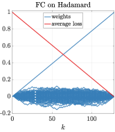
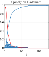
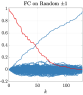
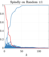
Figure 2: SGD on the Linear fully connected neuron (left) and spindly network (right) on Hadamard (top) and random $\pm 1$ matrices (bottom).

This second technique gives incomparable lower bounds. In particular it gives linear lower bounds when the instance matrix is random $\pm 1$ or $\{0,\!1\}$ or Gaussian instead of Hadamard. However the rank technique only applies to gradient descent trained fully connected linear neural networks of up to two layers. The rank $r$ is not easily bounded already for three layers. In contrast, the rank immediately becomes $d$ after seeing $\log d$ many examples when learning with the spindly network.

Curiously, the Hadamard problem can be seen as an exponential expansion of a cryptographically secure $\log d$ bit XOR problem (Bogdanov et al., 2019). This allows multiplicative updates and their gradient descent reparameterizations as the spindly network to learn this problem sample efficiently, while no expansion allows kernel method to avoid the linear lower bounds. We expand on this in Appendix D.

Previous work

The key idea of using squared weight parameters goes back to Gunasekar et al. (2017), who showed convergence of continuous gradient descent (CGD) on the squared weight reformulation to the minimum $\mathrm{L}_{1}$-norm solution in a matrix factorization context. The matrix analysis includes the spindly network as a special case where the factors are diagonal. It was shown later in (Amid and Warmuth, 2020a) that CGD on the spindly network equals to continuous unnormalized exponentiated gradient update (EGU) on a single neuron. Amid and Warmuth (2020b) also showed worst case regret bounds for the spindly network with discrete GD updates. These bounds closely match the original bound shown previously in (Kivinen and Warmuth, 1997) for EGU. In contrast, linear lower bounds for GD on a single linear neuron were shown in (Warmuth and Vishwanathan, 2005) when the instances are the $\pm 1$ valued rows of a Hadamard matrix and the target is a single feature. The linear behavior of SGD for single linear neurons holds experimentally even when the instances are random $[-1,1]^{d}$ or $[0,1]^{d}$ vectors. On the other hand, the regret bounds for the spindly network was shown for the case where instances are from the domain $[0,1]^{d}$. Nevertheless, the exponential decay of the average loss of SGD on the spindly network can be shown experimentally even when instances are random $[-1,1]^{d}$ vectors (see Figure 2 for a comparison). Note that Amid and Warmuth (2020b) discussed this observation only on an experimental level. Also, the domain mismatch in the upper and lower bounds was not addressed in the previous work. In order to close this gap, we extend the linear lower bound for a single linear neuron trained with GD to the case where the instances are in $[0,1]^{d}$. The technique for proving this type of lower bound (called second technique above) was originally introduced in (Warmuth and Vishwanathan, 2005). By averaging over targets, the linear lower bound was shown for learning Hadamard features even if the instances are embedded by an arbitrary $\phi$ map, thus showing that Hadamard features cannot be learned by any kernel method. This type of lower bound relies on the flat SVD spectrum of the Hadamard matrix. The spectrum of random $\pm 1$ matrices is also sufficiently flat to lead to a lower bound for any kernel methods. In this paper, we apply this second proof methodology to obtain similar linear lower bounds for GD trained 2-layer fully connected linear neural networks with arbitrary initialization.

Note that this paper is not per se about hardness results for learning certain unusual functions with neural networks (Telgarsky, 2016; Safran and Shamir, 2017). Instead we build on the work of Warmuth and Vishwanathan (2005); Warmuth et al. (2014) that study algorithms i.t.o. their invariance properties and prove linear lower bounds for rotation invariant algorithm (that include GD trained neural networks with fully connected input layers). These lower bounds can be bypassed by sparsifying the input layer (Figure 1).

Outline.

We begin with some basic definitions in Section 2 and proceed to prove our single feature lower bounds in Section 3. We then discuss the weaknesses of these bounds and then give extensions of the SVD based lower bound techniques (mostly relegated to the appendices). Open problems are discussed in the conclusion section.

2 Notations and setup

An example $(\bm{x},y)$ consists of a $d$-dimensional input vector $\bm{x}$ and real label $y$. We specify a learning problem as a tuple $(\underset{n,d}{\bm{X}},\underset{n}{\bm{y}})$ containing $d$ examples, where the rows of input matrix $\bm{X}$ are the $n$ (transposed) input vectors and the target $\bm{y}$ is a vector of their labels. For the sake of proving lower bounds, we will also consider learning problems having multiple targets $(\underset{n,d}{\bm{X}},\underset{n,m}{\bm{Y}})$, where now the columns of $\bm{Y}$ specify the separate targets. The training set always consists of the first $k\leq n$ examples of the problem $(\underset{k,d}{\bm{X}_{\text{tr}}},\underset{k}{\bm{y}_{\text{tr}}})=(\bm{X}_{1:k,:},\bm{y}_{1:k})$. If there is more than one target, then the labels must come from the same target, i.e. $\bm{y}=\bm{Y}\bm{e}_{i}$ for some $i=1,\ldots,m$ (where $\bm{e}_{i}$ is a vector with $1$ on the $i$-th coordinate, and zeros elsewhere).

A prediction algorithm is a real valued function $\hat{y}(\bm{x}\,|(\bm{X}_{\mathrm{tr}},\bm{y}_{\mathrm{tr}}))$ where $\bm{x}\in\mathbb{R}^{d}$ is the next input vector / test vector and $(\bm{X}_{\mathrm{tr}},\bm{y}_{\mathrm{tr}})$ the past training examples. With a slight abuse of the definition, we allow the function value of $\hat{y}$ to be randomized (a random variable), based on some internal randomness of the algorithm. The accuracy of prediction $\hat{y}$ on an example $(\bm{x},y)$ is measured by means of a square loss $(y-\hat{y})^{2}$.

Remark 2.1.

Our main lower bounds (Theorems 3.1 and 3.3) apply to a general class of losses $L(y,\hat{y})$, for which the only requirement is that when predicting a label $y\in\{+1,-1\}$, $\min_{\hat{y}}\frac{L(-1,\hat{y})+L(+1,\hat{y})}{2}$ is some positive constant $c$. Some of our lower bounds use $y\in\{0,1\}$ instead. In that case we need the requirement $\min_{\hat{y}}\frac{L(0,\hat{y})+L(1,\hat{y})}{2}$ is some positive constant $c^{\prime}$. For the lower bound to apply to a neural network training with gradient descent, we additionally need $L(y,\hat{y})$ to be differentiable in $\hat{y}$. Precisely, the constants $c$ or $c^{\prime}$ enter into the lower bounds. But this detail is a distraction and for the sake of concreteness, we state our theorems for the squared loss $L(y,\hat{y})=(y-\hat{y})^{2}$ (when $c=1$ and $c^{\prime}=\nicefrac{{1}}{{4}}$) and point out for when a linear lower bound still holds with the above weaker definition.

For the sake of simplicity, we avoid the discussion of randomized algorithms in the body of the paper by assuming that the loss is square loss and thus convex. In that case, any randomized algorithm $\hat{y}$ can be turned into a deterministic algorithm $\hat{y}_{\det}$:

$$\hat{y}_{\det}(\bm{x}|(\bm{X}_{\mathrm{tr}},\bm{y}_{\mathrm{tr}}))=\mathbb{E}\left[\hat{y}(\bm{x}|(\bm{X}_{\mathrm{tr}},\bm{y}_{\mathrm{tr}}))\right]\;\text{(expectation w.r.t. internal randomization)},$$

which by Jensen’s inequality has loss no greater than the expected loss of $\hat{y}$ on any instance:

$$(\hat{y}_{\det}(\bm{x}|(\bm{X}_{\mathrm{tr}},\bm{y}_{\mathrm{tr}}))-y)^{2}=\left(\mathbb{E}\left[\hat{y}(\bm{x}|(\bm{X}_{\mathrm{tr}},\bm{y}_{\mathrm{tr}}))\right]-y\right)^{2}\leq\mathbb{E}\left[\left(\hat{y}(\bm{x}|(\bm{X}_{\mathrm{tr}},\bm{y}_{\mathrm{tr}}))-y\right)^{2}\right].$$

A prediction algorithm $\hat{y}(\cdot\,|(\bm{X}_{\mathrm{tr}},\bm{y}_{\mathrm{tr}}))$ is called rotation invariant (Warmuth and Vishwanathan, 2005) if for any orthogonal matrix $\underset{d,d}{\bm{U}}$ and any input $\bm{x}\in\mathbb{R}^{d}$:

$$\hat{y}(\bm{U}\bm{x}|(\bm{X}_{\mathrm{tr}}\bm{U}^{\top},\bm{y}_{\mathrm{tr}}))=\hat{y}(\bm{x}|(\bm{X}_{\mathrm{tr}},\bm{y}_{\mathrm{tr}}))\,.$$ (1)

In other words, the prediction $\hat{y}(\bm{x},(\bm{X}_{\mathrm{tr}},\bm{y}_{\mathrm{tr}}))$ for any input $\bm{x}$ remains the same if we rotate both $\bm{x}$ and $\bm{X}_{\mathrm{tr}}$ by matrix $\bm{U}$. If the algorithm is randomized, then $\hat{y}$ is a random variable and the equality sign in definition (1) should be interpreted as “identically distributed”. Our lower bounds will be for a rotation invariant subclass of neural net algorithms.

In this paper, a neural network with a fully connected input layer is any real valued prediction function of the form $\hat{y}=N(\underset{d}{\bm{x}}^{\top}\underset{d,h}{\bm{W}},\bm{Z})$, where $\bm{x}$ is a real input vector, the $h$ columns of $\bm{W}$ are the weight vectors at the $h$ input neurons, and $\bm{Z}$ is a fixed set of additional weights (in the upper layers). We only require that $N$ must be differentiable in $\bm{W}$. Note that the parameters $(\bm{W},\bm{Z})$ naturally depend on the examples $(\bm{X}_{\operatorname{tr}},\bm{y}_{\operatorname{tr}})$.

We claim that a neural network is rotation invariant, if (i) it has a fully connected input layer in which (ii) each input node is initialized to zero or the input layer is initialized randomly to $\underset{d,h}{\bm{W}_{0}}$ which has a rotation invariant distribution, i.e. for any orthogonal matrix $\bm{U}$, $\bm{W}_{0}$ and $\bm{U}\bm{W}_{0}$ are identically distributed. Furthermore (iii), the input layer is updated with gradient descent on the training set $(\bm{X}_{\text{tr}},\bm{y}_{\text{tr}})$, and (iv) the updates of the additional weights $\bm{Z}$ depend on $\bm{X}_{\text{tr}}$ only through the outputs of the bottom layer $\bm{X}_{\text{tr}}\bm{W}$ (as in, e.g., gradient descent updates).

To prove this claim, let $\bm{W}_{t}$ and $\bm{Z}_{t}$ be the weights of the network after initializing at $\bm{W}_{0}$ and $\bm{Z}_{0}$ and running $t$ steps of gradient descent. We show that if the initial weight matrix and the training set are rotated by an orthogonal matrix $\bm{U}$, i.e., $\bm{W}_{0}\rightarrow\bm{U}\bm{W}_{0}$ and $\bm{X}_{\text{tr}}\rightarrow\bm{X}_{\text{tr}}\bm{U}^{\top}$, then the weights of the network undergo transformation $\bm{W}_{t}\rightarrow\bm{U}\bm{W}_{t}$ and $\bm{Z}_{t}\rightarrow\bm{Z}_{t}$ for all $t$. The latter is straightforward from the former and the fact that $\bm{Z}_{t}$ depend on $\bm{X}_{\text{tr}}$ only through $\bm{X}_{\text{tr}}\bm{W}_{j}$ $(j=0,\ldots,t-1)$, which remains invariant under $\bm{U}$: $\bm{X}_{\text{tr}}\bm{W}_{j}\rightarrow\bm{X}_{\text{tr}}\bm{U}^{\top}\bm{U}\bm{W}_{j}=\bm{X}_{\text{tr}}\bm{W}_{j}$.

To show $\bm{W}_{t}\rightarrow\bm{U}\bm{W}_{t}$ by induction on $t$, note that the gradient of the loss with respect to $\bm{W}_{t-1}$ on an example $(\bm{x},y)$ has the form $\bm{x}\bm{\delta}^{\top}$, where $\bm{\delta}=\nabla_{\bm{a}}N(\bm{a},\bm{Z}_{t-1})$ where $\bm{a}=\bm{x}^{\top}\bm{W}_{t-1}$ are the current linear activations at the input layer. Using the inductive hypothesis $\bm{W}_{t-1}\rightarrow\bm{U}\bm{W}_{t-1}$ and $\bm{Z}_{t-1}\rightarrow\bm{Z}_{t-1}$, every such linear activation $\bm{a}$ (and thus also $\bm{\delta}$) is invariant under $\bm{U}$ since $\bm{a}\rightarrow\bm{x}^{\top}\bm{U}^{\top}\bm{U}\bm{W}_{t-1}=\bm{x}^{\top}\bm{W}_{t-1}=\bm{a}$ and so the gradient undergoes a transformation $\bm{x}\bm{\delta}^{\top}\rightarrow\bm{U}\bm{x}\bm{\delta}^{\top}$. This let us conclude that $\bm{W}_{t}$ obtained from $\bm{W}_{t-1}$ by adding another gradients w.r.t. some examples from $(\bm{X}_{\text{tr}},\bm{y}_{\text{tr}})$ undergoes a transformation $\bm{W}_{t}\rightarrow\bm{U}\bm{W}_{t}$.

Hence the prediction of the rotated network on input $\bm{x}\rightarrow\bm{U}\bm{x}$ remains the same,

$$N(\bm{x}^{\top}\bm{U}^{\top}\bm{U}\bm{W}_{t},\bm{Z}_{t})=N(\bm{x}^{\top}\bm{W}_{t},\bm{Z}_{t}),$$

and the rotation invariance follows by recalling that $\bm{U}\bm{W}_{0}$ is distributed the same as $\bm{W}_{0}$.

3 Lower bounds for single target, any rotation invariant algorithm

Hadamard matrices are square $\pm 1$ matrices whose rows/columns are orthogonal. We assume the first row and column consists of all ones. We begin with a problem in which the instances are the rows of a $d$-dimensional Hadamard matrix and there is a single target ($m=1$), which is the constant function 1, i.e. the problem $(\underset{d,d}{\bm{H}},\underset{d,1}{\bm{1}})$. This is too easy, as any algorithm which always predicts $1$ has zero loss. So for each sign pattern ${\bm{s}}\in\{+1,-1\}^{d}$, consider the problem in which the rows of $\bm{H}$ and $\bm{1}$ are sign flipped by ${\bm{s}}$, i.e. the problem $(\operatorname{diag}({\bm{s}})\bm{H},{\bm{s}})$. Note that no matter what sign pattern ${\bm{s}}$ we use, the linear weight vector $\bm{e}_{1}$ has zero loss on this problem, as $\operatorname{diag}({\bm{s}})\bm{H}\bm{e}_{1}=\operatorname{diag}({\bm{s}})\bm{1}={\bm{s}}$. Since the sign pattern is chosen uniformly, the algorithm is unable to learn from the labels and needs to rely on the information in the inputs $\operatorname{diag}({\bm{s}})\bm{H}$. Below we show that no rotation invariant algorithm is able exploit this information beyond the training examples and thus can’t do better than random guessing on the unseen examples. See Appendix A for an informal proof for the neural net case.

Theorem 3.1.

For any rotation invariant algorithm receiving the first $k$ examples of the problem $(\operatorname{diag}({\bm{s}})\underset{d,d}{\bm{H}},{\bm{s}})$ where the random sign pattern ${\bm{s}}\in\{-1,+1\}^{d}$ is chosen uniformly, the expectation w.r.t. ${\bm{s}}$ of the average square loss on all $d$ examples is at least $1-\nicefrac{{k}}{{d}}$.

Proof 3.2.

We first rotate the instance matrix of all the $2^{d}$ sign flipped problems to a scaled identity matrix. Define a rotation matrix $\bm{U}_{\bm{s}}$ as $\nicefrac{{1}}{{\sqrt{d}}}\operatorname{diag}({\bm{s}})\bm{H}$. The predictions of any rotation invariant algorithm on $(\operatorname{diag}({\bm{s}})\bm{H},{\bm{s}})$ and $(\operatorname{diag}({\bm{s}})\bm{H}\bm{U}^{\top}_{\bm{s}},{\bm{s}})=(\sqrt{d}\bm{I},{\bm{s}})$ are the same. Note that the rotated linear weight of the target ${\bm{s}}$ is $\bm{U}_{\bm{s}}\bm{e}_{1}=\nicefrac{{1}}{{\sqrt{d}}}\,{\bm{s}}$.

Now fix ${\bm{s}}_{1:k}$. The algorithm receives the same first $k$ training examples for each problem $(\sqrt{d}\bm{I},{\bm{s}})$. Also since ${\bm{s}}_{(k+1):d}$ is chosen uniformly, each of the $d-k$ unseen examples is labeled $\pm 1$ with equal probability. So the best prediction on these $d\!-\!k$ examples is 0, incurring square loss at least 1 for each unseen example. We conclude that the expected average loss on all $d$ examples is at least $1-\nicefrac{{k}}{{d}}$.

Note that in this lower bound, the algorithms have square loss at least $\nicefrac{{1}}{{2}}$ at $k=\nicefrac{{d}}{{2}}$. An alternate related proof technique, sketched in Appendix B, flattens the lower bound curve using a duplication trick that moves the half point arbitrary far out. Also in Appendix C, we strengthen the above theorem in two ways: the loss is allowed to be any loss satisfying the property specified in Remark 2.1 and the input nodes can be randomly initialized as long as the distributions for choosing the initial weight vectors is rotation invariant.

Our next goal is to obtain a similar proof for the hardness of learning a constant function when the instance domain is $\{0,1\}^{d}$ instead of $\{-1,+1\}^{d}$. We do this because the upper bounds or EGU and its reparameterization with the spindly network require non-negative features. As for the above theorem, we only give a simplified version below, but this theorem can also be generalized using the techniques of Appendix C.

The function $\nicefrac{{(x+1)}}{{2}}$ shifts a $\pm 1$ variable $x$ to $0/1$. We essentially shift the previous proof using this transformation. For some reason which will become clear, we first need to remove the first row of $\bm{H}$ which is all 1. Let $\underset{d-1,d}{\bm{\widetilde{H}}}$ be the Hadamard matrix $\bm{H}$ with the first row removed. Our initial problem is now $\big{(}\nicefrac{{1}}{{2}}(\bm{\widetilde{H}}+\underset{\kern-2.84526ptd-1,d\kern-2.84526pt}{\bm{1}}),\underset{d-1}{\bm{1}}\big{)}$. Since $\bm{\widetilde{H}}\bm{1}=\bm{0}$ all $d-1$ rows of $\bm{\widetilde{H}}$ have an equal number of $\pm 1$’s and therefore the rows of $\nicefrac{{1}}{{2}}(\bm{\widetilde{H}}+\bm{1})$ have an equal number of $0/1$’s. Instead of doing random sign flipping of the rows as we did for $\bm{H}$, we now complement each row of $\nicefrac{{1}}{{2}}(\bm{\widetilde{H}}+\bm{1})$ with probability $\nicefrac{{1}}{{2}}$. If $\bm{h}$ is a row of $\bm{\widetilde{H}}$, then $\nicefrac{{1}}{{2}}(\pm\bm{h}+\bm{1})$ are two complementary rows of bits that are the shifted versions of $\pm\bm{h}$.

Theorem 3.3.

For any rotation invariant algorithm receiving the first $k$ examples of the problem $(\nicefrac{{1}}{{2}}(\operatorname{diag}({\tilde{{\bm{s}}}})\bm{\widetilde{H}}+\bm{1}),\nicefrac{{1}}{{2}}({\tilde{{\bm{s}}}}+\bm{1}))$ where the random sign pattern ${\tilde{{\bm{s}}}}\in\{-1,+1\}^{d-1}$ is chosen uniformly, the expectation w.r.t. ${\tilde{{\bm{s}}}}$ of the average square loss on all $d-1$ examples is at least $\frac{1}{4}(1-\frac{k}{d-1})$.

Proof 3.4.

We rotate the instance matrices of all the $2^{d-1}$ randomly complemented problems to a fixed matrix. Define a rotation matrix $\bm{U}_{\tilde{{\bm{s}}}}$ as $\nicefrac{{1}}{{\sqrt{d}}}\operatorname{diag}([1;{\tilde{{\bm{s}}}}])\bm{H}$. The predictions of any rotation invariant algorithm on the problems $(\nicefrac{{1}}{{2}}(\operatorname{diag}({\tilde{{\bm{s}}}})\bm{\widetilde{H}}+\bm{1}),\nicefrac{{1}}{{2}}({\tilde{{\bm{s}}}}+\bm{1}))$ and their rotations $(\nicefrac{{1}}{{2}}(\operatorname{diag}({\tilde{{\bm{s}}}})\bm{\widetilde{H}}+\bm{1})\bm{U}_{{\tilde{{\bm{s}}}}}^{\top},\nicefrac{{1}}{{2}}({\tilde{{\bm{s}}}}+\bm{1}))=(\nicefrac{{\sqrt{d}}}{{2}}[\underset{d-1,1}{\bm{1}},\underset{d-1,d-1}{\operatorname{diag}({\tilde{{\bm{s}}}})}],\nicefrac{{1}}{{2}}({\tilde{{\bm{s}}}}+\bm{1}))$ are the same. Note that the rotated linear weight of the target $\nicefrac{{1}}{{2}}({\tilde{{\bm{s}}}}+\bm{1})$ equals $\bm{U}_{{\tilde{{\bm{s}}}}}\bm{e}_{1}=\nicefrac{{1}}{{\sqrt{d}}}\,[1;{\tilde{{\bm{s}}}}]$.

Without loss of generality the algorithm receives the first $k$ examples of each rotated problem during training. Since ${\tilde{{\bm{s}}}}$ is chosen uniformly, each of the $d-1-k$ unseen examples is labeled $0/1$ with equal probability. So the best prediction on these $d-1-k$ examples is $\nicefrac{{1}}{{2}}$, incurring square loss at least $\nicefrac{{1}}{{4}}$ for each unseen example. Thus the expected average loss on all $d-1$ examples lower bounded by $\frac{d-1-k}{4\,(d-1)}=\frac{1}{4}(1-\frac{k}{d-1}).$

We next prove a lower bound for the Hadamard problem that was conjectured to be hard to learn by any neural network trained with gradient descent (Derezinski and Warmuth (2014)). The constant target is now any fixed column $\bm{h}$ of $\bm{H}$ other than the first one. We exploit that fact that $\bm{h}$ has an equal number of $\pm 1$ labels and randomly permute the rows of $\bm{H}$ and the target labels. The only available information to the rotation invariant algorithm are the $k$ labels seen in the training sample. Therefore, the best prediction the algorithm can be deduced from the average count of the remaining labels. On expectation, this gives a lower bound of $1-\frac{k}{d-1}$ on the average square loss, which is only slightly weaker than the bound of Theorem 3.1.

Theorem 3.5.

For any rotation invariant algorithm receiving the first $k$ examples of the problem $(\bm{\bm{P}}\bm{H},\bm{\bm{P}}\bm{h})$, where $\bm{h}=\bm{H}\bm{e}_{i}$ for some fixed $i\in\{2,\ldots,d\}$ is the $i$-th column of $\bm{H}$, and $\bm{\bm{P}}$ is a permutation matrix chosen uniformly at random, the expectation w.r.t. $\bm{\bm{P}}$ of the average square loss on all $d$ examples is at least $1-\frac{k}{d-1}$.

Proof 3.6.

Define a rotation matrix $\bm{U}$ as $\nicefrac{{1}}{{\sqrt{d}}}\,\bm{\bm{P}}\bm{H}$. The predictions of any rotation invariant algorithm on $(\bm{\bm{P}}\bm{H},\bm{\bm{P}}\bm{h})$ and $(\bm{\bm{P}}\bm{H}\bm{U}^{\top}\!,\bm{\bm{P}}\bm{h})=(\sqrt{d}\bm{I},\bm{\bm{P}}\bm{h})$ are the same. The algorithm receives the first $k$ examples of each problem $(\sqrt{d}\bm{I},\bm{\bm{P}}\bm{h})$ as training examples. Since the problems are permuted uniformly, every permutation of the unseen $d-k$ labels is equally likely. So the best prediction on the $d-k$ unseen labels is the average count of the unseen labels (which the algorithm can deduce from the count of the seen labels and the fact that $\bm{h}$ has an equal number of $\pm 1$ labels.) If we denote the number of unseen $+1/\!-1$ labels as $q$ and $(d-k)-q$, respectively, then the best prediction on all unseen labels is $\hat{y}=\frac{q-(d-k-q)}{d-k}$. The total square loss on all unseen examples is thus at least:

$$q(1-\hat{y})^{2}+(d-k-q)(-1-\hat{y})^{2}=\frac{4}{d-k}\;q(d-k-q).$$

In Appendix E we show that $q$ follows a hyper geometric distribution, by which we can compute the expected total loss as

$$\frac{4}{d-k}\;\mathbb{E}[q(d-k-q)]=d-\frac{kd}{d-1}.$$

Lower bounding the loss of the algorithm on seen examples by $0$, and dividing by $d$, the expected average loss over all $d-1$ examples is at least $1-\frac{k}{d-1}$.

3.1 Lower bound for random Gaussian inputs

The lower bounds in the previous section result from feeding a rotation invariant algorithm examples which are all orthogonal to each other. These type of problems might seem somewhat specialized and therefore in this section we show that rotation invariant algorithms are also unable to efficiently learn a simple class of problems in which the entries of $\bm{X}$ follow an i.i.d. standard Gaussian distribution, while the labels are generated noise-free by a sparse weight vector. On the other hand, this class of simple problems is perfectly learnable from just a single training example by a straightforward (non rotation invariant) algorithm.

We thus consider the problem matrix $(\bm{X},\bm{y})$, where the rows of $\bm{X}$ (instances) are generated i.i.d. from $N(\bm{0},\bm{I})$, while $\bm{y}=\bm{X}{\bm{w}}^{\star}$ for some ${\bm{w}}^{\star}$ with $\|{\bm{w}}^{\star}\|=1$. Note that the setup is noise-free as ${\bm{w}}^{\star}$ has zero loss on any such $(\bm{X},\bm{y})$. The standard Gaussian distribution is rotation invariant: if $\bm{x}\sim N(\bm{0},\bm{I})$ then $\bm{U}\bm{x}\sim N(\bm{0},\bm{I})$ for any orthogonal matrix $\bm{U}$. In fact, the whole analysis in this section would equally well apply to any rotation invariant distribution with covariance matrix $\bm{I}$, but we keep the Gaussian distribution for the sake of simplicity.

Theorem 3.7.

For any rotation invariant algorithm receiving the first $k$ examples of the problem $(\bm{X},\bm{y}\!=\!\!\bm{X}\!{\bm{w}}^{\star})$ for any $\|{\bm{w}}^{\star}\|=1$ with the $d$ rows of $\bm{X}$ being generated i.i.d. from $N(\bm{0},\bm{I})$, the expectation w.r.t. $\bm{X}$ of the average square loss on all $d$ examples is at least $(1-\nicefrac{{k}}{{d}})^{2}$.

This lower bound $(1-\nicefrac{{k}}{{d}})^{2}=1-2\,\nicefrac{{k}}{{d}}+(\nicefrac{{k}}{{d}})^{2}$ is slightly weaker than the ones for orthogonal instances. Yet the algorithm has expected loss at least $\nicefrac{{1}}{{4}}$ after seeing half of the examples.

Proof 3.8.

(sketch, full proof in Appendix F) We first show that a rotation invariant algorithm has the same expected average loss for any ${\bm{w}}^{\star}$ with $\|{\bm{w}}^{\star}\|=1$, as both the data and ${\bm{w}}^{\star}$ can be rotated without changing the data distribution or the predictions of the algorithm. Then we consider a problem in which ${\bm{w}}^{\star}$ itself is drawn uniformly from a unit sphere, and show that every algorithm (not necessarily rotation invariant) has expected average loss at least $(1-\nicefrac{{k}}{{d}})^{2}$ on all examples where the expectation is taken with respect to a random choice of ${\bm{w}}^{\star}$ and $\bm{X}$. It then follows from the first argument that a rotation invariant algorithm has expected average loss at least $(1-\nicefrac{{k}}{{d}})^{2}$ for any choice of ${\bm{w}}^{\star}$.

Since the loss of a rotation invariant algorithm does not depend on the choice of the target weight vector ${\bm{w}}^{\star}$, one can choose any fixed sparse vector ${\bm{w}}^{\star}=\bm{e}_{i}$ for $i\in\{1,\ldots,d\}$ as the target. In each case the algorithm still incurs expected loss at least $(1-\nicefrac{{k}}{{d}})^{2}$ on average after seeing $k$ examples. On the other hand for a Gaussian input matrix, sparse weight vectors are easy to learn from a single example. This is because for ${\bm{w}}^{\star}=\bm{e}_{i}$, the label coincides with the $i$-th input feature and each entry of every row of $\bm{X}$ is unique with probability one.

We note that the lower bound of Theorem 3.7 is tight and matched by the (rotation invariant) least squares algorithm (proof in Appendix G).

Theorem 3.9.

Consider the problem $(\bm{X},\bm{y}=\bm{X}{\bm{w}}^{\star})$ for any $\|{\bm{w}}^{\star}\|=1$ where the columns of $\bm{X}$ generated i.i.d. from $N(\bm{0},\bm{I})$. The least squares algorithm, which upon seeing $k$ examples, predicts with the weight vector ${\bm{w}}=\bm{X}_{1:k,:}^{\dagger}\bm{y}_{1:k}$, where $\bm{A}^{\dagger}$ denotes the pseudo-inverse of $\bm{A}$, has expected average loss $(1-\nicefrac{{k}}{{d}})^{2}$ on all $d$ examples, where the expectation is w.r.t. the random choice of $\bm{X}$.

4 Shortcomings of single target lower bound technique of Theorem 3.1

1. The rotation invariant initialization of the fully connected input nodes is necessary: If all input nodes were initialized to $\bm{e}_{1}$, then the network would learn with zero examples because

   $$\underbrace{s_{i}\bm{h}_{i}}_{\kern-14.22636pt\text{sign flipped $i$-th instance}\kern-14.22636pt}\cdot\;\;\;\underbrace{\bm{e}_{1}}_{{\bm{w}}_{0}}=s_{i}.$$

2. The lower bound is also broken if the instances are embedded by an arbitrary feature map $\mathbb{R}^{d}\ni\bm{x}\mapsto\phi(\bm{x})\in\mathbb{R}^{m}$, as allowed by kernel methods. For example, all rows of $\bm{H}$ can be embedded as the same row, $\phi(\bm{h}_{i})=\bm{e}_{1}$. Now after the fully connected input nodes all receive the sign flipped first instance $s_{1}\bm{e}_{1}$ as their input, we are essentially in the target initialized case.

3. Most of all the lower bounds shown so far mostly require the instances to be orthogonal. We already showed that random Gaussian features lead to a slightly weaker lower bound for sparse targets (Theorem 3.7). However ideally we want lower bounds when the features are random $\pm 1$.

In the next section we show that in a special case, the initialization ${\bm{w}}_{0}=\bm{0}$ can be shown to be optimal. We then expand the SVD based lower bounding technique of Warmuth and Vishwanathan (2005) which covers the case of arbitrary initialization and random $\pm 1$ features. However so far, all of this only works for linear neural networks with up to two fully connected layers.

5 Zero initial weight vector is optimal for a single linear neuron

Theorem 5.1.

Consider learning the problem $(\bm{H},[\bm{1},-\bm{1}])$ on a single linear neuron with any initialization ${\bm{w}}_{0}$. Assume the algorithm updates with gradient descent based on the first $k$ instances. Then the average square loss over all $d$ instances and both targets is at least $1-\nicefrac{{k}}{{d}}$ and is minimized when ${\bm{w}}_{0,k+1:d}=\bm{0}$.

Proof 5.2.

Since the algorithm is rotation invariant, it is convenient to switch to proving the lower bound for problem matrix $(\sqrt{d}\,\bm{I},[\bm{1},-\bm{1}])\text{ and any }{\bm{w}}_{0}$. For both targets, the algorithms weight vector is ${\bm{w}}_{0}$ plus a linear combination of the first $k$ instances $\sqrt{d}\bm{e}_{i}$, i.e. ${\bm{w}}={\bm{w}}_{0}+[\underset{1,k}{\bm{b}},\underset{1,d-k}{\bm{0}}]^{\top}$, where $\bm{b}$ depends on the target. For any unseen instance $\sqrt{d}\bm{e}_{j}$ for $j>i$, the linear neuron predicts $\sqrt{d}\bm{e}_{j}^{\top}{\bm{w}}=\sqrt{d}w_{0,j}$ on both targets when the label is $\bm{e}_{j}^{\top}(\pm\bm{1})=\pm 1$. So the average loss is at least

$$\nicefrac{{1}}{{2d}}\sum_{j=k+1}^{d}\underbrace{\Big{(}(\sqrt{d}w_{0,i}-1)^{2}+(\sqrt{d}w_{0,i}+1)^{2}\Big{)}}_{\text{minimized when $w_{0,j}=0$}}\;\geq\;\frac{1}{2d}\;2(d-k)\;=\;1-\frac{k}{d}.$$

This proves that the initialization $w_{0,j}=0$ is optimal for all $j>k$.

This type of lower bounds does not work for a single target (say $\bm{1}$) because ${\bm{w}}_{0}$ could be set to generate this target and no loss would be incurred. By additionally permuting the rows of $\bm{H}$, we can force all components of ${\bm{w}}_{0}$ to 0.

6 SVD based lower bounds for linear neural nets

An alternative second technique for deriving lower bounds for learning the Hadamard problem using GD uses the SVD spectrum of the design matrix (Warmuth and Vishwanathan, 2005). The main idea is to lower bound the loss on all examples averaged over all targets based on the tail sum of the squared singular values of a matrix $\bm{Y}$ containing the label vectors of all targets as columns. The instances are the transposed rows of $\underset{n,d}{\bm{Y}}$, transformed by an arbitrary feature map $\phi\!:\!\mathbb{R}^{d}\!\!\rightarrow\!\mathbb{R}^{m}.\!$ We first present this technique in its simplest form.

Theorem 6.1 ((Warmuth and Vishwanathan, 2005)).

For any $\phi$ map, the average square loss for learning the problem $(\underset{n,m}{\phi(\bm{Y})},\underset{n,d}{\bm{Y}})$ after seeing any $0\leq k\leq\text{rank}(\bm{Y})$ training instances and using GD on a single linear neuron with zero initialization is lower bounded by $\frac{1}{\|\bm{Y}\|_{\text{F}}^{2}}\sum_{i=k+1}^{\text{rank}(\bm{Y})}s_{i}^{2},$ where $s_{i}$ is the $i$-th singular value of $\bm{Y}$ in the decreasing order.

Proof 6.2.

For a fixed target column $\bm{y}_{i}$ of $\bm{Y}$ and after seeing $k$ arbitrary rows $\underset{k,m}{\phi(\widehat{\bm{Y}})}$, the weight vector of the GD algorithm can be written as a linear combination of these rows, i.e. ${\bm{w}}=\phi(\widehat{\bm{Y}})^{\top}\bm{a}_{j}$ for some $\bm{a}_{j}\in\mathbb{R}^{k}$. We can now write the average square loss as

$$\frac{1}{\|\bm{Y}\|_{\text{F}}^{2}}\sum_{j\in[d]}\|\phi(\bm{Y})\phi(\widehat{\bm{Y}})^{\top}\bm{a}_{j}-\bm{y}_{j}\|^{2}=\frac{1}{\|\bm{Y}\|_{\text{F}}^{2}}\,\|\overbrace{\phi(\bm{Y})\underbrace{\phi(\widehat{\bm{Y}})^{\top}\!}_{m,k}\underset{k,d}{\bm{A}}}^{\text{rank-}k}-\bm{Y}\|_{\text{F}}^{2}\geq\frac{1}{\|\bm{Y}\|_{\text{F}}^{2}}\sum_{i=k+1}^{\text{rank}(\bm{Y})}s_{i}^{2}\,,$$

where $\bm{A}$ is the matrix with $j$-th column equal to $\bm{a}_{j}$.

Notice that the above relies on the fact that for any rank $0\leq k\leq\text{rank}(\bm{Y})$, the square loss of any rank $k$ approximation of matrix $\bm{Y}$ is lower bounded by the sum of the smallest $\text{rank}(\bm{Y})-k$ squared singular values of $\bm{Y}$. As a result, the bound is effective only when $\bm{Y}$ has a flat spectrum. The original bound of Theorem 6.1 was proposed for learning the $d$-dimensional Hadamard matrix $\bm{Y}=\bm{H}$ with $n=d$. In this case $\|\bm{H}\|_{\text{F}}^{2}=d^{2}$, $\text{rank}(\bm{H})=d$, and all $d$ singular values $s_{i}^{2}$ are equal to $d$. Thus the lower bound reduces to $\frac{1}{d^{2}}(d-k)d=1-\frac{k}{d}$, for $0\leq k\leq d$. When $\bm{Y}$ contains random $\pm 1$ features, then the tail of a square spectrum is tightly concentrated and the lower bound becomes $1\!-\!\frac{ck}{d}$ where $c\!>\!0$ (Appendix I).

We next observe that with any (fixed) initialization ${\bm{w}}_{0}$ of the single neuron, the rank of weight matrix goes up by one and the lower bound becomes $\frac{1}{\|\bm{Y}\|_{F}^{2}}\sum_{i=k+1+1}^{\text{rank}(\bm{Y})}s_{i}^{2}$. We show this for a doubled version of the Hadamard problem, with targets $\pm\bm{h}_{j}$ for $j\in[n]$, because this helps with the proof of the next theorem.

Theorem 6.3.

For any $\phi$ map, the average square loss for learning the problem $(\phi(\bm{H}),[\bm{H},-\bm{H}])$ after seeing any $0\leq k\leq d$ training instances and using GD on a single linear neuron with any initialization is lower bounded by $1-\frac{k+1}{d}$.

Proof 6.4.

Similar to the proof of Theorem 6.1, we have

$$\frac{1}{2d^{2}} \|\!\overbrace{\phi(\bm{H})(\underset{m,k}{\phi(\widehat{\bm{H}})^{\top}}\!\!\bm{A}+\underset{m,1}{{\bm{w}}_{0}}\,\underset{1,2d}{\bm{1}^{\top}})}^{\text{rank $k+1$}}-[\bm{H},\!-\bm{H}]\|_{\text{F}}^{2}=\frac{1}{2d^{2}}\!\!\!\sum_{i=k+2}^{d}\!\!\!s_{i}^{2}=\frac{(d\!-\!(k\!+\!1))(2d)}{2d^{2}}=1\!-\!\frac{k\!+\!1}{d}\,.\vspace{-5mm}$$

The above lower bound is not directly comparable with the available upper bounds for the spindly network which require the input features and labels to be in a the range $[0,X]$ and $[0,Y]$, respectively, for some constants $X,Y>0$. However we can shift the $\pm 1$ features of $\bm{Y}$ to $0/1$ as was done for Theorem 3.3. The spectrum essentially remains flat.

Essentially we need to compute the SVD spectrum of $\underset{d,2d}{\bm{M}}\coloneqq([\bm{H},-\bm{H}]\,+\underset{d,2d}{\bm{1}})/2$. Matrix $\bm{M}$ has rank at least $d$, thus we have $\text{rank}(\bm{M})=d$ and all rows of $\bm{M}$ have equal number ($d$ many) $1$’s and $0$’s. Thus $\|\bm{M}\|_{\text{F}}^{2}=d^{2}$. Note that we have

$$\bm{M}\,\bm{M}^{\top} =([\bm{H},-\bm{H}]+\underset{d,2d}{\bm{1}})/2\quad([\bm{H},-\bm{H}]+\underset{d,2d}{\bm{1}})^{\top}/2=(2d\,\underset{d,d}{\bm{I}}+2\,\underset{d,d}{\bm{0}}+2d\,\underset{d,d}{\bm{1}})/4=\frac{d}{2}(\underset{d,d}{\bm{I}}+\underset{d,d}{\bm{1}}).$$

Recall that the $s_{i}^{2}$ of $\bm{M}$ are the eigenvalues of $\bm{M}\,\bm{M}^{\top}$ sorted in decreasing order. The following shows the eigensystem of $\bm{M}\,\bm{M}^{\top}$ is $\frac{\bm{H}}{\sqrt{d}}$ and also gives its eigenvalues:

$$\frac{\bm{H}^{\top}}{\sqrt{d}}\;\frac{d}{2}(\underset{d,d}{\bm{I}}+\underset{d,d}{\bm{1}})\;\frac{\bm{H}}{\sqrt{d}} =\bm{H}^{\top}(\underset{d,d}{\bm{I}}+\underset{d,d}{\bm{1}})\bm{H}/2=(\bm{H}^{\top}+d\;[\bm{1};\underset{d-1,1}{\bm{0}}]^{\top})\;\bm{H}/2$$

$$=\frac{d}{2}\,\underset{d,d}{\bm{I}}+\frac{d^{2}}{2}\operatorname{diag}([1,\underbrace{0,\ldots,0}_{d-1}])=\operatorname{diag}([\frac{d^{2}}{2}\!+\!\frac{d}{2},\underbrace{\frac{d}{2},\ldots,\frac{d}{2}}_{d-1}])\,,$$

where we use the fact that the first row and column of $\bm{H}$ has all ones and all remaining rows and columns have an equal number of $\pm 1$’s. The following lower bound carries immediately.

Corollary 6.5.

For any $\phi$ map, the average square loss for learning the problem $(\phi(\bm{H}),([\bm{H},$
$-\bm{H}]+\bm{1})/2)$ after seeing any $0\leq k\leq d$ training instances and using GD on a single linear neuron with any initialization is lower bounded by $\frac{1}{2d^{2}}(d-k-1)\frac{d}{2}=\frac{1}{4}-\frac{k+1}{4d}.$

We now consider a two-layer network with fully connected linear layers having weights $\underset{m,h}{\bm{W}^{(1)}}$ and $\underset{h,1}{{\bm{w}}^{(2)}}$, respectively, where $m$ is the input dimension and $h$ is the number of hidden units. Assume we are learning the problem $(\bm{X}\!=\!\phi(\bm{Y}),\bm{Y})$ with gradient descent based on the first $k$ training examples $(\bm{X}_{\text{tr}}\!=\!\bm{X}_{1:k,:},\bm{y}_{\text{tr}}\!=\!\bm{y}_{1:k})$.

Theorem 6.6.

After seeing $k$ training examples $(\bm{X}_{\text{tr}},\bm{y}_{\text{tr}})$, GD training keeps the combined weight $\bm{W}^{(1)}{\bm{w}}^{(2)}$ in the span of $[\bm{W}_{0}^{(1)}{\bm{w}}_{0}^{(2)},\bm{W}_{0}^{(1)}(\bm{W}_{0}^{(1)})^{\top}\bm{X}_{\text{tr}}^{\top},\bm{X}_{\text{tr}}]$, which is rank $\leq 2k+1$.

The above rank bound (proven in Appendix H) immediately gives a lower bound of $1-\frac{2k+1}{d}$ for $(\phi(\bm{H}),\bm{H})$. We conjecture the lower bound can be improved to $1-\frac{k+1}{d}$ (which is observed experimentally). Since the rank bound of $2k+1$ can be tight, we see that the rank argument gets weak. For three layers the rank goes up too quickly for this methodology to be useful.

7 Conclusion

We show in this paper that GD trained neural networks with a fully connected input layer and rotation invariant initialization at the input nodes cannot sample efficiently learn single components. Most of our lower bounds use the rows of Hadamard matrices as instances which use $\pm 1$ features. We show a slightly weaker but still linear lower bound when the features are Gaussian and conjecture that the same weaker lower bound also holds for random $\pm 1$ features..

It would also be interesting to further investigate the power of fully connected linear networks. We made some progress by extending the SVD based method of Warmuth and Vishwanathan (2005) which provides linear lower bounds for learning the components of random $\pm 1$ matrices even when the instances are transformed with an arbitrary $\phi$ map and when an arbitrary initialization is used. For this method it is necessary to bound the rank of a certain weight matrix, but we were only able to do this for up to two fully connected layers. Note that all lower bounds on GD trained neural nets with complete input layers are for a fixed target component when no transformation is used. We conjecture that the same linear lower bounds hold for arbitrary transformations if we average over target components. However, totally different proof techniques would be needed to prove this conjecture.

Finally, there are many technical open problems regarding the GD training of the spindly network (Figure 1): Do the regret bounds still hold when the domain is $[-1,1]^{d}$ instead of $[0,1]^{d}$? Is clipping of the predictions necessary? Experimentally the network still learns efficiently if all $2d$ weight are initialized with random positive numbers or if the $d$ bottom weights are initialized to 0. However the regret bounds of (Amid and Warmuth, 2020b) do not hold for these cases.

Acknowledgments

Thanks to Vishy Vishwanathan for many inspiring discussions and for letting us include the concentration theorem of Appendix I which is due to him. This research was partially support by NSF grant IIS-1546459.

Appendix A Informal proof of Theorem 3.1 for the case of GD trained neural nets with a complete input layer

The problem $(\bm{H},\bm{1})$, i.e. learning the constant target 1 when the instances are the (transposed) orthogonal rows of the Hadamard matrix $\underset{d,d}{\bm{H}}$, is too easy. So we feed the net randomly sign flipped rows $(s\bm{h}^{\top},s)$, for $s=\pm 1$, where $\bm{h}$ is a row of $\bm{H}$ in the training set. The neural net has a complete input layer that is trained with gradient descent. So the weights at the input nodes are linear combinations of the $k$ seen instances. Thus the input nodes are “no help” for predicting the labels of the unseen examples since they are orthogonal to the seen ones. Also the labels of the seen examples are random and thus do not contain any information for predicting the label of the unseen examples. The unseen sign flipped instances are labeled $\pm 1$ with equal probability. So the optimum prediction of the unseen $d-k$ examples is 0, and we incur one unit of square loss for each. The loss on the seen examples is non-negative and thus the total average loss on all $d$ examples is at least $\frac{d\!-\!k}{d}\!=\!1\!-\!\frac{k}{d}$. $\blacksquare$

Appendix B Alternate proof style related to Theorem 3.1 that interleaves duplicated positive and negative rows of Hadamard.

Instead of using sign flipped rows of $\bm{H}$, we use the following instance matrix: Matrix $\bm{X}_{q}$ (for $q\geq 1$) consists of $q$ copies of the first row of $\bm{H}$, followed by $q$ copies of minus the first row, $q$ copies of the second, $q$ copies of minus the second, $\ldots$, for a total of $2q\,d$ rows. The label vector $\bm{y}_{q}$ is again the first column of $\bm{X}_{q}$, i.e. it consists of alternating blocks of $(+1)^{q}$ and $(-1)^{q}$. After receiving the first $k$ examples of $(\bm{X}_{q},\bm{y}_{q})$, LLS has average loss

$$1-\frac{2q\lceil{\frac{k}{2q}}\rceil}{2q\,d}\,,$$ (2)

on all $2q\,d$ examples because it predicts 0 on all unseen block pairs. (See saw tooth curve in Figure 3 in which each tooth drops by $\nicefrac{{1}}{{d}}$ and then stays flat for $2q-1$ steps). Also if each pair $1\leq i\leq d$ of blocks is randomly swapped, i.e. the $q$ rows of minus row $i$ come before the $q$ rows of plus row $i$, then after receiving $k$ examples, the expected average square loss is lower bounded by the same saw tooth curve, where the expectation is w.r.t. $d$ random swaps.

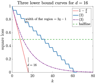
Figure 3: Bound of Thm. 3.1 (dotted) & bounds for sampling from $(\bm{X}_{2},\!\bm{y}_{2})$ w.o. replacement (solid) and i.i.d. (dash-dot).

This is because in that case the optimal prediction for any GD trained neural network on all unseen blocks is 0 (proof not shown). This $q$ “duplication trick” moves the point where the loss is half to $k=q\,d$ and the loss 0 point to $k=2q\,d$ (See Figure 3).

Also note that training on the first $k$ examples of random permutations of $(\bm{X}_{q},\bm{y}_{q})$ for large $q$ approximates sampling with replacement on this type of problem. Again the optimal algorithm must predict zero on all $i$, s.t. row $i$ nor minus row $i$ have not been sampled yet. We believe that our sampling w.o. replacement lower bounds are more succinct, because they avoid the coupon collector problem for collecting the $d$ row pairs: For the sake of completeness, the expected square loss after picking $k$ i.i.d. examples from $(\bm{X}_{1},\bm{y}_{1})$ is

$$(1-\nicefrac{{1}}{{d}})^{k},$$ (3)

which is the expected number of pairs not collected yet (See plot in Figure 3 for comparison).

Appendix C Proof of Theorem 3.1 for losses that only require the property from Remark 2.1

Here we extend Theorem 3.1 to arbitrary losses which only satisfy the property in Remark 2.1. Since we do not assume convexity of the loss, we need to consider a randomized rotation invariant algorithm (as the randomized algorithms are no longer dominated by deterministic ones). Formally, let ${\bm{\theta}}$ denote a collection of random variables (independent of the data), which represent the internal randomization of the algorithms. Given the training sample $(\bm{X}_{\mathrm{tr}},\bm{y}_{\mathrm{tr}})$ and the input $\bm{x}$, the prediction of the algorithm is a random variable $\hat{y}_{{\bm{\theta}}}(\bm{x}|(\bm{X}_{\mathrm{tr}},\bm{y}_{\mathrm{tr}}))$. The algorithm is rotation invariant if for any orthogonal matrix $\bm{U}$,

$$\hat{y}_{{\bm{\theta}}}(\bm{x}|(\bm{X}_{\mathrm{tr}},\bm{y}_{\mathrm{tr}})) \hat{y}_{{\bm{\theta}}}(\bm{U}\bm{x}|(\bm{X}_{\mathrm{tr}}\bm{U}^{\top},\bm{y}_{\mathrm{tr}}))\,,$$ and (4)

are identically distributed.

In the context of neural networks, the random variables ${\bm{\theta}}$ consist of the random initialization $\bm{W}_{0}$ as well as additional random variables used by the algorithm. We assume that ${\bm{\theta}}$ is not affected by rotating the instances. Also as in the deterministic algorithm case, if the weights $\bm{W}$ at the bottom layer are updated with gradient descent, then rotating the instances causes the weights $\bm{W}$ to be counter rotated and the predictions stay unchanged.

We now continue with the general proof using assumption (4) for the case of Theorem 3.1. Take a problem $(\operatorname{diag}({\bm{s}})\bm{H},{\bm{s}})$ with the sign pattern ${\bm{s}}\in\{-1,+1\}^{d}$ chosen uniformly at random, and assume the algorithm has received its first $k$ examples, $(\bm{X}_{1:k,:},{\bm{s}}_{1:k})$. Define a rotation matrix $\bm{U}_{{\bm{s}}}=\nicefrac{{1}}{{\sqrt{d}}}\;\text{diag}({\bm{s}})\bm{H}$. The expected total loss of the algorithm on the unseen examples is

$$\mathrm{expected~{}loss} =\mathbb{E}_{{\bm{s}}}\mathbb{E}_{{\bm{\theta}}}\left[\sum_{t=k+1}^{d}L\big{(}s_{t},\hat{y}_{{\bm{\theta}}}(\bm{x}_{t}|(\bm{X}_{1:k,:},{\bm{s}}_{1:k}))\big{)}\right]$$

$$\stackrel{{\scriptstyle(*)}}{{=}}\mathbb{E}_{{\bm{s}}}\mathbb{E}_{{\bm{\theta}}}\left[\sum_{t=k+1}^{d}L\big{(}s_{t},\hat{y}_{{\bm{\theta}}}(\bm{U}_{{\bm{s}}}\bm{x}_{t}|(\bm{X}_{1:k,:}\bm{U}_{{\bm{s}}}^{\top},{\bm{s}}_{1:k}))\big{)}\right]$$

$$=\mathbb{E}_{{\bm{s}}}\mathbb{E}_{{\bm{\theta}}}\left[\sum_{t=k+1}^{d}L\big{(}s_{t},\hat{y}_{{\bm{\theta}}}(\sqrt{d}\bm{e}_{t}|(\sqrt{d}\bm{I}_{1:k,:},{\bm{s}}_{1:k}))\big{)}\right]$$

$$=\mathbb{E}_{{\bm{\theta}}}\mathbb{E}_{{\bm{s}}_{1:k}}\mathbb{E}_{{\bm{s}}_{(k+1):d}|{\bm{s}}_{1:k}}\left[\sum_{t=k+1}^{d}L\big{(}s_{t},\hat{y}_{{\bm{\theta}}}(\sqrt{d}\bm{e}_{t}|(\sqrt{d}\bm{I}_{1:k,:},{\bm{s}}_{1:k}))\big{)}\right]$$

$$\geq\mathbb{E}_{{\bm{\theta}}}\mathbb{E}_{{\bm{s}}_{1:k}}\left[\frac{1}{2}\sum_{t=k+1}^{d}\min_{\hat{y}\in\mathbb{R}}\left\{L\big{(}-1,\hat{y})+L\big{(}+1,\hat{y})\right\}\right]$$

$$=(d-k)\min_{\hat{y}\in\mathbb{R}}\left\{\frac{1}{2}(L\big{(}-1,\hat{y})+L\big{(}+1,\hat{y}))\right\}\geq(d-k)c,$$

where in $(*)$ we used the rotation invariance of the algorithm and the last inequality follows from Remark 2.1. Lower bounding the loss of the algorithm on seen examples by zero, the average expected loss of the rotation invariant algorithm is at least $\nicefrac{{1}}{{d}}\,(d-k)c=(1-\nicefrac{{k}}{{d}})c$. $\blacksquare$

It is worthwhile to check if the lower bounds for Hadamard data also hold for other type of randomization beyond rotation invariance. As an interesting example, consider reflective invariant distributions. The distribution $P$ is reflective invariant if $\forall\;{\bm{\theta}},P({\bm{\theta}})=P(-{\bm{\theta}})$. The question is whether a lower bound can be proven for a neural network trained with a gradient descent method, when the random initialization of the weights is reflective invariant. Unfortunately this is not the case: Let the randomness ${\bm{\theta}}$ correspond to a random intialization of the weight vector ${\bm{w}}_{0}=(s,0,\ldots,0)$, with $s\in\{-1,1\}$ generated uniformly at random (so  ${\bm{w}}_{0}=s{\bm{w}}^{\star}$). This is a reflective invariant initialization. On the first training example $\bm{x}_{1}$, the bottom neurons evaluate to ${\bm{w}}_{0}^{\top}\bm{x}_{1}=sy_{1}$, so the upper layers (getting $y_{1}$ as feedback) can in principle learn to multiply the result by $s$ again to get $\hat{y}_{1}=y_{1}$. On unseen examples $\bm{x}_{i}$, the bottom neurons again evaluate to ${\bm{w}}^{\top}\bm{x}_{i}={\bm{w}}_{0}^{\top}\bm{x}_{i}=sy_{i}$, and multiplying by $s$ by upper layers gives zero loss.

Appendix D Hadamard matrix as an exponential expansion

The simplest way to construct Hadamard matrices of dimension $d=2^{q}$ is to use the following recursive construction credited to Sylvester (Sylvester, 1867):

$$\bm{H}_{1}=[1],\quad\bm{H}_{2}=\begin{bmatrix}1&1\\ 1&-1\end{bmatrix},\ldots,\quad\bm{H}_{q+1}=\begin{bmatrix}\;\bm{H}_{q}&\;\bm{H}_{q}\\ \;\bm{H}_{q}&-\bm{H}_{q}\end{bmatrix}\,.$$

Note that the first row and column of these matrices only consists of $+1$’s. We make use of this convenient fact in the paper.

Curiously enough this matrix is an expansion of all $\log d$ $\pm 1$ bit patterns to $2^{d}$ product features. For example, for $d=3$:

$$d\overbrace{\left\{\begin{pmatrix}+&+&+\\ -&+&+\\ +&-&+\\ -&-&+\\ +&+&-\\ -&+&-\\ +&-&-\\ -&-&-\end{pmatrix}\right.}^{\log d}\;\stackrel{{\scriptstyle{\psi}}}{{\longrightarrow}}\;\overbrace{\begin{pmatrix}+&+&+&+&+&+&+&+\\ +&-&+&-&+&-&+&-\\ +&+&-&-&+&+&-&-\\ +&-&-&+&+&-&-&+\\ +&+&+&+&-&-&-&-\\ +&-&+&-&-&+&-&+\\ +&+&-&-&-&-&+&+\\ +&-&-&+&-&+&+&-\end{pmatrix}}^{d}$$

$b_{1}$
$b_{2}$
$b_{3}$
$1$
$b_{1}$
$b_{2}$
$b_{1}b_{2}$
$b_{3}$
$b_{1}b_{3}$
$b_{2}b_{3}$
$b_{1}b_{2}b_{3}$

Now observe that the XOR product features are hard to learn by any time efficient algorithm from the $\log d$ bit patterns when the features are noisy. However the above exponential expansion $\psi$ makes it possible for the EGU algorithm or the GD trained spindly network to crack this cryptographically hard problem using essentially $\log d$ examples (albeit in time that is exponential in $\log d$). In the noisy case, the number of examples also only grows with $\log d$ (Amid and Warmuth (2020b)). Note that $\log d$ is also the Vapnik Chervonienkis dimension of the XOR problem.

Can kernel based algorithm also learn this noisy XOR problem? First observe that the dot product between two size $d$, $\psi$-expanded feature vectors (i.e. rows of the Hadamard matrix) can be computed in $O(\log d)$ time using the following reformulation of the dot product:

$${\psi}(\bm{b})\!\cdot\!{\psi}(\mathbf{\tilde{b}})=\sum_{I\subseteq 1..\log d}\;\prod_{i\in I}b_{i}\tilde{b}_{i}\;=\;\prod_{i=1}^{\log d}(1\!+\!b_{i}\tilde{b}_{i})\,.$$

This looks promising! However already in (Warmuth and Vishwanathan, 2005) it was shown that the Hadamard problem (a reformulation of the XOR problem as seen above) cannot be learned in a sample efficient way by any kernel method using any kernel feature map $\phi$ (including the above one): After receiving $k$ of the $d$ examples, the averaged loss on all $d$ example is at least $1-\nicefrac{{k}}{{d}}$. The key in these lower bounds is to average over features and examples, and also exploit the fact that the weight space of kernel method has low rank and the SVD spectrum of the problem matrix $\bm{H}$ is flat: $\log d\,\underset{d,1}{\bm{1}}$. In this paper we greatly expand this proof methodology in Section 6. Notice that before the expansion, the SVD spectrum of the $d\times\log d$ matrix of all bit patterns has the much shorter flat SVD spectrum of $\log d\;\underset{\log d,1}{\bm{1}}$.

Appendix E Completing the proof of Theorem 3.5

Since the target $\bm{h}$ has an equal number of $\pm$ labels, the number of positive unseen labels $q$ is a random variable which follows a hyper geometric distribution, i.e. the number of successes in $d-k$ draws without replacement from a population of size $d$ that contains $\nicefrac{{d}}{{2}}$ successes. Thus the mean and variance are

$$\mathbb{E}[q]=\frac{d-k}{2}\quad\text{and}\quad\mathrm{Var}(q)=\frac{(d-k)k}{4(d-1)}=\mathbb{E}[q^{2}]-(\mathbb{E}[q])^{2}\,.$$

The expected total loss on all unseen examples is thus at least

$$\frac{4}{d-k}\mathbb{E}[q(d-k-q)] =\frac{4}{d-k}(\mathbb{E}[q](d-k)-\mathbb{E}[q^{2}])$$

$$=\frac{4}{d-k}\left(\frac{(d-k)^{2}}{2}-\mathrm{Var}(q)-\frac{(d-k)^{2}}{4}\right)$$

$$=(d-k)-\frac{k}{d-1}=d-\frac{kd}{d-1}\,.$$

$\blacksquare$

Appendix F Proof of Theorem 3.7

We start by showing that a rotation invariant algorithm has the same average expected (with respect to a random draw of $\bm{X}$) loss for any ${\bm{w}}^{\star}$ with $\|{\bm{w}}^{\star}\|=1$. Indeed take two such vectors ${\bm{w}}^{\star}_{1}$ and ${\bm{w}}^{\star}_{2}$ and note that there exists an orthogonal transformation $\bm{U}$ such that ${\bm{w}}^{\star}_{2}=\bm{U}{\bm{w}}^{\star}_{1}$. Due to rotation invariance of the Gaussian distribution, the instance matrix $\bm{X}$ has the same distribution as the instance matrix $\bm{X}\bm{U}^{\top}$, and thus the average expected loss of any algorithm on problem $(\bm{X},\bm{X}{\bm{w}}^{\star}_{1})$ and $(\bm{X}\bm{U}^{\top},\bm{X}\bm{U}{\bm{w}}^{\star}_{1})=(\bm{X}\bm{U}^{\top},\bm{X}{\bm{w}}^{\star}_{2})$ is the same. Additionally, if the algorithm is rotation invariant, its predictions (and thus the average loss) on the problems $(\bm{X}\bm{U}^{\top},\bm{X}{\bm{w}}^{\star}_{2})$ and $(\bm{X}\bm{U}^{\top}\bm{U},\bm{X}{\bm{w}}^{\star}_{2})=(\bm{X},\bm{X}{\bm{w}}^{\star}_{2})$ are the same. Thus, we conclude that a rotation invariant algorithm has the same average expected loss on $(\bm{X},\bm{X}{\bm{w}}^{\star}_{1})$ and $(\bm{X},\bm{X}{\bm{w}}^{\star}_{2})$.

We now consider a problem in which ${\bm{w}}^{\star}$ itself is drawn uniformly from a unit sphere in $\mathbb{R}^{d}$, and show that every algorithm (not necessarily rotation invariant) has average expected loss at least $(1-\nicefrac{{k}}{{d}})^{2}$ on all examples (where the expectation is with respect to a random choice of ${\bm{w}}^{\star}$ and $\bm{X}$). It then follows from the previous paragraph that a rotation invariant algorithm has average expected loss at least $(1-\nicefrac{{k}}{{d}})^{2}$ for any choice of ${\bm{w}}^{\star}$.

Thus, let ${\bm{w}}^{\star}$ be drawn uniformly from a unit sphere. The covariance matrix of ${\bm{w}}^{\star}$ is $c\bm{I}$ from the spherical symmetry of the distribution, and $c$ is easily shown to be $\nicefrac{{1}}{{d}}$:

$$cd=\operatorname{tr}(c\bm{I})=\operatorname{tr}\left(\mathbb{E}\left[{\bm{w}}^{\star}{\bm{w}}^{\star}{}^{\top}\right]\right)=\mathbb{E}\left[\operatorname{tr}({\bm{w}}^{\star}{\bm{w}}^{\star}{}^{\top})\right]=\mathbb{E}\left[\|{\bm{w}}^{\star}\|^{2}\right]=\mathbb{E}[1]=1\,.$$

Let $(\bm{X}_{1:k,:},\bm{y}_{1:k})$ be a subset of $k$ examples seen by the algorithm. Take any unseen example $\bm{x}_{i}$ ($i>k$). Decompose the loss of the algorithm on this example as $\mathbb{E}[(y_{i}-\hat{y}_{i})]=\mathbb{E}[y_{i}^{2}-2\hat{y}_{i}y_{i}+\hat{y}^{2}]$, where the expectation is over both ${\bm{w}}^{\star}$ and $\bm{X}$. The first term is easy to calculate:

$$\mathbb{E}[y_{i}^{2}]=\mathbb{E}[\bm{x}_{i}^{\top}{\bm{w}}^{\star}{\bm{w}}^{\star}{}^{\top}\bm{x}_{i}]=\mathbb{E}[\bm{x}_{i}^{\top}\underbrace{\mathbb{E}_{{\bm{w}}^{\star}}[{\bm{w}}^{\star}{\bm{w}}^{\star}{}^{\top}]}_{=\bm{I}/d}\bm{x}_{i}]=\frac{1}{d}\mathbb{E}[\|\bm{x}_{i}\|^{2}]=\frac{d}{d}=1\,,$$

where we used the fact that $\mathbb{E}[\|\bm{x}_{i}\|^{2}]=\operatorname{tr}(\mathbb{E}[\bm{x}_{i}\bm{x}_{i}^{\top}])=\operatorname{tr}(\bm{I})=d$.

For the second term, decompose ${\bm{w}}^{\star}={\bm{w}}_{\|}+{\bm{w}}_{\perp}$, into the part within the span of the seen examples (rows of $\bm{X}_{1:k,:}$), and the part orthogonal to the span: ${\bm{w}}_{\|}\in\text{span}\{\bm{X}_{1:k,:}\}$, ${\bm{w}}_{\perp}\perp\text{span}\{\bm{X}_{1:k,:}\}$. Note that ${\bm{w}}^{\star}={\bm{w}}_{\|}+{\bm{w}}_{\perp}$ has the same distribution as ${\bm{w}}^{-\star}={\bm{w}}_{\|}-{\bm{w}}_{\perp}$. The is easily seen if we eigen decompose $\bm{X}_{1:k,:}^{\top}\bm{X}_{1:k,:}=\sum_{j=1}^{r}\lambda_{i}\bm{v}_{j}\bm{v}_{j}^{\top}$, where $r=\mathrm{rank}(\bm{X}_{1:k,:})\leq k$, and form an orthogonal matrix $\bm{U}=2\sum_{j=1}^{r}\bm{v}_{j}\bm{v}_{j}^{\top}-\bm{I}$. Since $\bm{v}_{j}^{\top}{\bm{w}}_{\perp}=0$ for any $j\leq r$ and ${\bm{w}}_{\|}\in\mathrm{span}(\bm{v}_{1},\ldots,\bm{v}_{r})$,

$$\bm{U}{\bm{w}}^{\star}=\bm{U}{\bm{w}}_{\|}+\bm{U}{\bm{w}}_{\perp}={\bm{w}}_{\|}-{\bm{w}}_{\perp}={\bm{w}}^{-\star}\,,$$

so the two vectors are rotations of each other, therefore having the same distribution. Note that the prediction of the algorithm $\hat{y}_{i}$ does not depend on ${\bm{w}}_{\perp}$, because the labels $\bm{y}_{\|}$ observed by the algorithm only depend on ${\bm{w}}_{\|}$: $y_{j}=\bm{x}_{j}^{\top}{\bm{w}}^{\star}=\bm{x}_{j}^{\top}{\bm{w}}_{\|}$ for any $\bm{x}_{j}\in\text{span}\{\bm{X}_{1:k,:}\}$. Thus:

$$\mathbb{E}[\hat{y}_{i}\,y_{i}] =\mathbb{E}[\hat{y}\,\bm{x}_{i}^{\top}{\bm{w}}^{\star}]=\frac{1}{2}\mathbb{E}[\hat{y}\bm{x}_{i}^{\top}\,({\bm{w}}^{\star}+{\bm{w}}^{-\star})]=\frac{1}{2}\mathbb{E}[2\,\hat{y}\,\bm{x}_{i}^{\top}{\bm{w}}_{\|}]$$

$$=\mathbb{E}[\hat{y}\,\bm{x}_{\|}^{\top}{\bm{w}}_{\|}]=\mathbb{E}[\hat{y}\,\bm{x}_{\|}^{\top}{\bm{w}}^{\star}]\,,$$

where $\bm{x}_{\|}$ is a projection of $\bm{x}_{i}$ onto $\text{span}\{\bm{X}_{1:k,:}\}$, and we used the facts that $\bm{x}_{i}^{\top}{\bm{w}}_{\|}=(\bm{x}_{\|}+\bm{x}_{\perp})^{\top}{\bm{w}}_{\|}=\bm{x}_{\|}^{\top}{\bm{w}}_{\|}$ and similarly that $\bm{x}_{\|}^{\top}{\bm{w}}^{\star}=\bm{x}_{\|}^{\top}({\bm{w}}_{\|}+{\bm{w}}_{\perp})=\bm{x}_{\|}^{\top}{\bm{w}}_{\|}$. This gives:

$$\mathbb{E}[(y_{i}-\hat{y}_{i})^{2}]=\mathbb{E}[y_{i}^{2}-2\hat{y}_{i}y_{i}+\hat{y}_{i}^{2}]=1+\mathbb{E}\left[\hat{y}_{i}^{2}-2\,\hat{y}_{i}\,\bm{x}_{\|}^{\top}{\bm{w}}^{\star}\right]\,.$$

The term under expectation is minimized for $\hat{y}_{i}=\bm{x}_{\|}^{\top}{\bm{w}}^{\star}$:

$$\mathbb{E}[(y_{i}-\hat{y}_{i})]\geq 1-\mathbb{E}[(\bm{x}_{\|}^{\top}{\bm{w}}^{\star})^{2}]\,.$$

We now upper bound the last expectation:

$$\mathbb{E}[(\bm{x}_{\|}^{\top}{\bm{w}}^{\star})^{2}]=\mathbb{E}[\bm{x}_{\|}^{\top}\underbrace{\mathbb{E}_{{\bm{w}}^{\star}}[{\bm{w}}^{\star}{\bm{w}}^{\star}{}^{\top}]}_{=\bm{I}/d}\bm{x}_{\|}]=\frac{1}{d}\,\mathbb{E}[\|\bm{x}_{\|}\|^{2}]\leq\frac{k}{d}\,.$$

The last inequality follows from the fact that when conditioning on $\bm{X}_{1:k,:}$ and taking expectation with respect to $\bm{x}_{i}$:

$$\mathbb{E}_{\bm{x}_{i}}[\|\bm{x}_{\|}\|^{2}]=\sum_{j=1}^{r}\mathbb{E}_{\bm{x}_{i}}\left[(\bm{v}_{j}^{\top}\bm{x}_{i})^{2}\right]=\sum_{j=1}^{r}\bm{u}_{j}^{\top}\underbrace{\mathbb{E}_{\bm{x}_{i}}[\bm{x}_{i}\bm{x}_{i}^{\top}]}_{=\bm{I}}\bm{u}_{j}=\sum_{i=1}^{r}\|\bm{u}_{j}\|^{2}=r\,,$$

where $r=\mathrm{rank}(\bm{X}_{1:k,:})$ and $\{\bm{u}_{1},\ldots,\bm{u}_{r}\}$ are the eigenvectors of $\bm{X}_{1:k,:}^{\top}\bm{X}_{1:k,:}$ with non-zero eigenvalues (which form a basis for $\mathrm{span}(\bm{X}_{1:k,:})$). As $\bm{x}_{i}$ was chosen arbitrarily, the expected loss on every unseen example is thus at least $1-\frac{k}{d}$. Lower bounding the loss on the seen examples by zero, the average expected loss is at least

$$\frac{1}{d}\left(0\cdot k+\left(1-\frac{k}{d}\right)\cdot(d-k)\right)=\left(1-\frac{k}{d}\right)^{2}\,.$$

Appendix G Proof of Theorem 3.9 (optimality of least-squares)

The least squares algorithm predicts with

$${\bm{w}}=\bm{X}_{1:k,:}^{\dagger}\bm{y}_{1:k}=\bm{X}_{1:k,:}^{\dagger}\bm{X}_{1:k,:}{\bm{w}}^{\star}\,.$$

Note that $\bm{X}_{1:k,:}^{\dagger}\bm{X}_{1:k,:}$ is an orthogonal projection onto span of $\bm{X}_{1:k,:}\,$. Let $\bm{P}=\bm{I}-\bm{X}_{1:k,:}^{\dagger}\bm{X}_{1:k,:}$ be the complementary projection. For any unseen example $\bm{x}_{i}$, the algorithm predicts with $\hat{y}_{t}=\bm{x}_{i}^{\top}{\bm{w}}$ and incurs loss

$$(y_{i}-\hat{y}_{i})^{2}=(\bm{x}_{i}^{\top}{\bm{w}}^{\star}-\bm{x}_{i}^{\top}\bm{X}_{1:k,:}^{\dagger}\bm{X}_{1:k,:}{\bm{w}}^{\star})^{2}=(\bm{x}_{i}^{\top}\bm{P}{\bm{w}}^{\star})^{2}={\bm{w}}^{\star}{}^{\top}(\bm{P}\bm{x}_{i}\bm{x}_{i}^{\top}\bm{P}){\bm{w}}^{\star}\,.$$

Taking expectation over $\bm{x}_{i}$:

$$\mathbb{E}_{\bm{x}_{i}}[(y_{i}-\hat{y}_{i})^{2}]={\bm{w}}^{\star}{}^{\top}(\bm{P}\underbrace{\mathbb{E}_{\bm{x}_{i}}[\bm{x}_{i}\bm{x}_{i}^{\top}]}_{=\bm{I}}\bm{P}){\bm{w}}^{\star}={\bm{w}}^{\star}\bm{P}{\bm{w}}^{\star}\,,$$

where we used $\bm{P}\bm{P}=\bm{P}$ from the properties of the projection operator. Taking expectation over $\bm{X}_{1:k,:}$ we get $\mathbb{E}[\bm{P}]=c\bm{I}$, for some constant $c\geq 0$, due to spherical symmetry of the distribution of $\bm{X}$. The constant $c$ can be evaluated to $\frac{d-k}{d}$ by:

$$cd=\operatorname{tr}(c\bm{I})=\operatorname{tr}(\mathbb{E}[\bm{P}])=\mathbb{E}[\operatorname{tr}(\bm{P})]=\mathbb{E}[\mathrm{rank}(\bm{P})]=d-k\,,$$

where we used the fact that due to spherical symmetry of the distribution, with probability one all rows in $\bm{X}$ are in general positions and thus any $d-k$ rows of $\bm{X}$ span a subspace of rank $d-k$. Thus the loss on any unseen example is given by $\mathbb{E}[(y_{i}-\hat{y}_{i})^{2}]=\frac{d-k}{d}\|{\bm{w}}^{\star}\|^{2}=\frac{d-k}{d}$, while the loss on every seen example is zero, as $\bm{x}_{i}^{\top}{\bm{w}}=\bm{x}_{i}^{\top}\bm{X}_{1:k,:}^{\dagger}\bm{X}_{1:k,:}{\bm{w}}^{\star}=\bm{x}_{i}^{\top}{\bm{w}}^{\star}=y_{i}$ for any $i\in\{1,\ldots,k\}$. Thus, the total loss expected loss on all examples is $(d-k)(1-\nicefrac{{k}}{{d}})$, which translates to the average expected loss of $\big{(}1-\frac{k}{d}\big{)}^{2}$.

Appendix H Proof of Theorem 6.6

Consider a two-layer network with fully connected linear layers having weights $\underset{d,h}{\bm{W}^{(1)}}$ and $\underset{h,1}{{\bm{w}}^{(2)}}$ where $d$ is the input dimension and $h$ is the number of hidden units. Given input $\underset{k,d}{\bm{X}_{\text{tr}}}\!=\!\bm{X}_{1:k,:}$ and target $\underset{k,1}{\bm{y}_{\text{tr}}}\!=\!\bm{y}_{1:k}$, we consider the square loss $\nicefrac{{1}}{{2}}\,\|\underbrace{\bm{X}_{\text{tr}}\bm{W}^{(1)}\,{\bm{w}}^{(2)}-\bm{y}_{\text{tr}}}_{\coloneqq\underset{k,1}{\bm{\delta}}}\|^{2}$. The following theorem characterized the column span of the combined weights $\bm{W}^{(1)}{\bm{w}}^{(2)}$ after seeing examples in $\bm{X}_{\text{tr}}$.

Theorem H.1.

Let $\underset{d,h}{\bm{W}_{0}^{(1)}}$ and $\underset{h,1}{{\bm{w}}_{0}^{(2)}}$ be the initial weights of a two layer fully connected linear network. After seeing examples $\bm{X}_{\text{tr}}$ with GD training on any target $\bm{y}_{\text{tr}}$, the weights have the form $\bm{W}^{(1)}=\bm{W}_{0}^{(1)}+\bm{X}_{\text{tr}}^{\top}(\bm{A}\,\bm{X}_{\text{tr}}\,\bm{W}_{0}^{(1)}+\bm{a}\,({\bm{w}}_{0}^{(2)})^{\top})$ and ${\bm{w}}^{(2)}=c{\bm{w}}_{0}^{(2)}+(\bm{W}_{0}^{(1)})^{\top}\bm{X}_{\text{tr}}^{\top}\bm{b}$ for some $c\in\mathbb{R}$, $\underset{k,d}{\bm{A}}$, $\underset{k,1}{\bm{a}}$, and $\underset{k,1}{\bm{b}}$.

Proof H.2.

The proof proceeds by induction on the updates (we used tilde to denote objects after the update):

$$\widetilde{\bm{W}}^{(1)} =\bm{W}^{(1)}-\eta\nabla_{\bm{W}^{(1)}}L$$

$$=\bm{W}^{(1)}-\eta\bm{X}_{\text{tr}}^{\top}\bm{\delta}({\bm{w}}^{(2)})^{\top}$$

$$=\bm{W}^{(1)}-\eta\bm{X}_{\text{tr}}^{\top}\bm{\delta}(c{\bm{w}}_{0}^{(2)}+(\bm{W}_{0}^{(1)})^{\top}\bm{X}_{\text{tr}}^{\top}\bm{b})^{\top}$$

$$=\bm{W}_{0}^{(1)}+\bm{X}_{\text{tr}}^{\top}(\underbrace{(\bm{A}-\eta\bm{\delta}\bm{b}^{\top})}_{\widetilde{\bm{A}}}\bm{X}_{\text{tr}}\bm{W}_{0}^{(1)}+\underbrace{(\bm{a}-c\eta\bm{\delta})}_{\widetilde{\bm{a}}}\,({\bm{w}}_{0}^{(2)})^{\top})\,,$$

$$\widetilde{{\bm{w}}}^{(2)} ={\bm{w}}^{(2)}-\eta\nabla_{{\bm{w}}^{(2)}}L$$

$$={\bm{w}}^{(2)}-\eta(\bm{W}^{(1)})^{\top}\bm{X}_{\text{tr}}^{\top}\bm{\delta}$$

$$=c{\bm{w}}_{0}^{(2)}+(\bm{W}_{0}^{(1)})^{\top}\bm{X}_{\text{tr}}^{\top}\bm{b}-\Big{(}\eta(\bm{W}_{0}^{(1)})^{\top}+\eta\,((\bm{W}_{0}^{(1)})^{\top}\bm{X}_{\text{tr}}^{\top}\bm{A}^{\top}+{\bm{w}}_{0}^{(2)}\,\bm{a}^{\top})\bm{X}_{\text{tr}}\Big{)}\bm{X}_{\text{tr}}^{\top}\bm{\delta}$$

$$=\underbrace{(c-\eta\,\bm{a}^{\top}\bm{X}_{\text{tr}}\bm{X}_{\text{tr}}^{\top}\bm{\delta})}_{\widetilde{c}}\,{\bm{w}}_{0}^{(2)}+(\bm{W}_{0}^{(1)})^{\top}\bm{X}_{\text{tr}}^{\top}\underbrace{(\bm{b}-\eta\,(\bm{I}+\bm{A}^{\top}\bm{X}_{\text{tr}})\bm{X}_{\text{tr}}^{\top}\bm{\delta})}_{\widetilde{\bm{b}}}\,.$$

Proof H.3.

​​of Theorem 6.6  We simply combine the observations of Theorem H.1:

$$\bm{W}^{(1)}{\bm{w}}^{(2)} =\big{(}\bm{W}_{0}^{(1)}+\bm{X}_{\text{tr}}^{\top}(\bm{A}\,\bm{X}_{\text{tr}}\,\bm{W}_{0}^{(1)}+\bm{a}\,({\bm{w}}_{0}^{(2)})^{\top})\big{)}\big{(}c{\bm{w}}_{0}^{(2)}+(\bm{W}_{0}^{(1)})^{\top}\bm{X}_{\text{tr}}^{\top}\bm{b}\big{)}$$

$$=c\bm{W}_{0}^{(1)}{\bm{w}}_{0}^{(2)}+\bm{W}_{0}^{(1)}(\bm{W}_{0}^{(1)})^{\top}\bm{X}_{\text{tr}}^{\top}\bm{b}+\bm{X}_{\text{tr}}^{\top}(\bm{A}\,\bm{X}_{\text{tr}}\,\bm{W}_{0}^{(1)}+\bm{a}\,({\bm{w}}_{0}^{(2)})^{\top}){\bm{w}}^{(2)},$$

which lies in the span of $[\bm{W}_{0}^{(1)}{\bm{w}}_{0}^{(2)},\bm{W}_{0}^{(1)}(\bm{W}_{0}^{(1)})^{\top}\bm{X}_{\text{tr}}^{\top},\bm{X}_{\text{tr}}]$.

Note that if $\bm{W}_{0}^{(1)}(\bm{W}_{0}^{(1)})^{\top}=\underset{d,d}{\bm{I}}$ for $d\geq h$, then $\bm{W}^{(1)}{\bm{w}}^{(2)}$ lies in the column span of $[\bm{W}_{0}^{(1)}{\bm{w}}_{0}^{(2)},\bm{X}_{\text{tr}}^{\top}]$ and the rank becomes at most $k+1$. Alternatively for $\bm{W}_{0}^{(1)}=\bm{0}$, then $\bm{W}^{(1)}{\bm{w}}^{(2)}$ lies in the column span of $\bm{X}_{\text{tr}}^{\top}$ which has rank at most $k$.

In general however, the rank argument for linear fully connected neural networks becomes weaker when the number of layers is increased to $3,4,\ldots,$ while experimentally, the average loss does not improve but increasing the number of layers.

Appendix I Concentration of SVD spectrum of random $\pm 1$ matrices

Using techniques from (Davidson and Szarek, 2003) and (Meckes, 2004), we will show that the sum of the last $d-k$ square singular values of a random $d\times d$ $\pm 1$ matrix is concentrated around $1-c\frac{k}{d}$, where $c>0$ is a constant independent of $d$.

Theorem I.1.

Let $\operatorname{\mathbf{M}}\in\{\pm 1\}^{d\times d}$ be a random matrix and $s_{1}\geq s_{2}\ldots\geq s_{d}$ denote its singular values. Then, there is a constant $c_{E}\geq 1$ that does not depend on $d$ such that for all $t\geq c\approx 7.09$,

$$P\left[\frac{1}{d^{2}}\sum_{i=k+1}^{d}s_{i}^{2}\geq 1-\frac{k}{d}\left(c_{E}+\frac{t}{\sqrt{d}}\right)^{2}\right]\geq 1-4\;\exp(-\frac{(t-c)^{2}}{4})\,.$$ (5)

So for $t=\sqrt{d}$, the theorem says that the probability that $Q$ is at least $1-c^{\prime}\frac{k}{d}$ (for some constant $c^{\prime}$ independent of $d$) is exponentially close to 1.

The following intermediate theorem bounds the expectation and median of the largest singular values of a random $\pm 1$ matrix. It also shows the concentration of the matrix norm around its median. We use $\operatorname{\mathbb{E}}[X]$ and $\operatorname{\mathbb{M}}[X]$ to denote the expectation and median of a random variable $X$. Recall that the probability of a random variable taking a value below the median is at most $0.5$.

Theorem I.2 ((Davidson and Szarek, 2003; Meckes, 2004)).

Let $\operatorname{\mathbf{M}}\in\{\pm 1\}^{d\times d}$ be a random matrix, $s_{1}\geq s_{2}\ldots\geq s_{d}$ denote its singular values, $E:=\operatorname{\mathbb{E}}[s_{1}]$, and $M:=\operatorname{\mathbb{M}}[s_{1}]$. Then

$$\sqrt{d}\leq E\leq c_{E}\sqrt{d}\mbox{ and }\sqrt{d}\leq M\leq c_{M}\sqrt{d}\,,$$ (6)

where $c_{E},c_{M}\geq 1$ are constants that do not depend on $d$. We also have that for all non-negative $t$,

$$P\left[\,|s_{1}-M|\geq t\right]\leq 4\exp(-t^{2}/4)\,.$$ (7)

Since $s_{1}$ is highly concentrated around its median, the following corollary shows that it is also highly concentrated around its mean:

Corollary I.3.

Let $\operatorname{\mathbf{M}}$, $E$, $M$, and $s_{i}$ as above. Then for all $t\geq c=4^{\frac{3}{2}}\Gamma(\frac{3}{2})\approx 7.09$,

$$P\left[\,|s_{1}-E|\geq t\right]\leq 4\exp(-(t-c)^{2}/4)\,.$$

Proof I.4.

By definition of expectation and Eq. (7)

$$|E-M|=|\operatorname{\mathbb{E}}[s_{1}]-M| \leq\operatorname{\mathbb{E}}|s_{1}-M|$$

$$:=\int_{0}^{\infty}P\left[\,|s_{1}-M|\geq t\right]\,dt$$

$$\leq 4\int_{0}^{\infty}\exp(-t^{2}/4)\,dt=4^{\frac{3}{2}}\Gamma(\frac{3}{2})=c\,.$$

Using Eq. (7) and the above inequality

$$P\left[\,|s_{1}-E|\geq t\right] \leq P\left[\,|s_{1}-M|+|M-E|\geq t\right]$$

$$\leq P\left[\,|s_{1}-M|\geq t-c\right]$$

$$\leq 4\exp(-(t-c)^{2}/4)\,.$$

We are now ready to prove Theorem I.1 which shows that, with high probability, the SVD spectrum of $\operatorname{\mathbf{M}}$ does not decay rapidly.

Proof of Theorem I.1: From the previous corollary, using $E,t\geq 0$, we have

$$P[s_{1}^{2}<(E+t)^{2}] \geq P[E-t<s_{1}<E+t]$$

$$\geq 1-4\exp(-(t-c)^{2}/4)\,,$$

and hence

$$P[d^{2}-ks_{1}^{2}>d^{2}-k(E+t)^{2}]\geq 1-4\exp(-(t-c)^{2}/4)\,.$$ (8)

The fact that $s_{1}\geq s_{2}\ldots\geq s_{d}$ and $\sum_{i}s_{i}^{2}=||\operatorname{\mathbf{M}}||^{2}_{F}:=\sum_{i,j}|M_{i,j}|^{2}=d^{2}$, jointly imply that $\sum_{i>k}s_{i}^{2}\geq d^{2}-ks_{1}^{2}$. Using this and Eq. (8), we obtain

$$P\left[\frac{1}{d^{2}}\sum_{i=k+1}^{d}s_{i}^{2}\geq 1-\frac{k}{d^{2}}(E+t)^{2}\right]\geq 1-4\exp(-(t-c)^{2}/4)\,.$$

Since $E\leq c_{E}\sqrt{d}$ (see Eq.(6)), the LHS of the above inequality is upper bounded by $P\left[\frac{1}{d^{2}}\sum_{i=k+1}^{d}s_{i}^{2}\geq 1-\frac{k}{d}\left(c_{E}+\frac{t}{\sqrt{d}}\right)^{2}\right]$ and the theorem follows.

References

• Amid and Warmuth (2020a) Ehsan Amid and ManfredΒ K. Warmuth. Reparameterizing mirror descent as gradient descent. arXiv preprint arXiv:2002.10487, 2020a. To appear Advances in Neural Information Processing Systems (NeurIPS).
• Amid and Warmuth (2020b) Ehsan Amid and ManfredΒ K Warmuth. Winnowing with gradient descent. In Conference on Learning Theory (COLT), pages 163–182. PMLR, 2020b.
• Bogdanov etΒ al. (2019) Andrej Bogdanov, Manuel Sabin, and PrashantΒ Nalini Vasudevan. XOR codes and sparse learning parity with noise. In Proceedings of the 2019 Annual ACM-SIAM Symposium on Discrete Algorithms, pages 986–1004, 2019.
• Davidson and Szarek (2003) K.Β R. Davidson and S.Β J. Szarek. Local operator theory, random matrices and banach spaces. In J.Β Lindenstrauss and W.Β Johnson, editors, Handbook of the Geometry of Banach Spaces, volumeΒ 1, chapterΒ 8, pages 317–366. North-Holland, Amsterdam, 2003.
• Derezinski and Warmuth (2014) Michal Derezinski and ManfredΒ K. Warmuth. The limits of squared Euclidean distance regularization. In Advances in Neural Information Processing Systems (NeurIPS), pages 2807–2815, 2014.
• Gunasekar etΒ al. (2017) Suriya Gunasekar, BlakeΒ E Woodworth, Srinadh Bhojanapalli, Behnam Neyshabur, and Nati Srebro. Implicit regularization in matrix factorization. In Advances in Neural Information Processing Systems (NeurIPS), pages 6151–6159, 2017.
• Kamath etΒ al. (2020) Pritish Kamath, Omar Montasser, and Nathan Srebro. Approximate is good enough: Probabilistic variants of dimensional and margin complexity. In Conference on Learning Theory (COLT), pages 163–182. PMLR, 2020.
• Kivinen and Warmuth (1997) Jyrki Kivinen and ManfredΒ K. Warmuth. Exponentiated gradient versus gradient descent for linear predictors. Information and Computation, 132(1):1–63, 1997.
• Maass and Warmuth (1998) M.Β Maass and M.K. Warmuth. Efficient learning with virtual threshold gates. Information and Computation, 141(1):66–83, February 1998.
• Meckes (2004) M.Β W. Meckes. Concentration of norms and eigenvalues of random matrices. Journal of Functional Analysis, 211(2):508–524, June 2004.
• Safran and Shamir (2017) Itay Safran and Ohad Shamir. Depth-width tradeoffs in approximating natural functions with neural networks. In International Conference on Machine Learning (ICML), pages 2979–2987, 2017.
• Sylvester (1867) J.J. Sylvester. Thoughts on inverse orthogonal matrices, simultaneous signsuccessions, and tessellated pavements in two or more colours, with applications to Newton’s rule, ornamental tile-work, and the theory of numbers. The London, Edinburgh, and Dublin Philosophical Magazine and Journal of Science, 34(232):461–475, 1867.
• Tao (2012) Terence Tao. Topics in Random Matrix Theory. American Mathematical Society, 2012.
• Telgarsky (2016) Matus Telgarsky. Benefits of depth in neural networks. In Conference on Learning Theory (COLT), pages 1517–1539, 2016.
• Warmuth etΒ al. (2014) M.Β K. Warmuth, W.Β KotΕ‚owski, and S.Β Zhou. Kernelization of matrix updates. Journal of Theoretical Computer Science, 558:159–178, 2014. Special issue for the 23nd International Conference on Algorithmic Learning Theory (ALT).
• Warmuth and Vishwanathan (2005) M.K. Warmuth and S.V.N. Vishwanathan. Leaving the span. In Proceedings of the 18th Annual Conference on Learning Theory (COLT), 2005.