Algodynamics: Interactive Transition System approach to Step-wise Refinement in the Design of Algorithms

Algodynamics: Teaching Algorithms using Interactive Transition Systems

Abstract.

The importance of algorithms and data structures in computer science curricula has been amply recognized. For many students, however, gaining a good understanding of algorithms remains a challenge.

Because of the automated nature of sequential algorithms there is an inherent tension in directly applying the ‘learning by doing’ approach. This partly explains the limitations of efforts like algorithm animation and code tracing.

Algodynamics, the approach we propose and advocate, situates algorithms within the framework of transition systems and their dynamics and offers an attractive approach for teaching algorithms. Algodynamics starts with the premise that the key ideas underlying an algorithm can be identified and packaged into interactive transition systems. The algorithm when ‘opened up’, reveals a transition system, shorn of most control aspects, enriched instead with interaction. The design of an algorithm can be carried out by constructing a series of interactive systems, progressively trading interactivity with automation. These transition systems constitute a family of notional machines.

We illustrate the algodynamics approach by considering Bubblesort. A sequence of five interactive transition systems culminate in the classic Bubblesort algorithm. The exercise of constructing the individual systems also pays off when coding Bubblesort: a highly modular implementation whose primitives are borrowed from the transition systems. The transition systems used for Bubblesort have been implemented as interactive experiments. These web based implementations are easy to build. The simplicity and flexibility afforded by the algodynamics framework makes it an attractive option to teach algorithms in an interactive way.

1. Introduction

Algorithms in the ACM curriculum

Algorithms form an essential component of recommended curricula in computer science(Joint Task Force on Computing Curricula and Society, 2013), computer engineering(Impagliazzo et al., 2003) and software engineering(on Computing Curricula, 2015). On the other hand, students continue to face difficulty with algorithmic problem solving: in problem formulation, notation for expressing solutions, logical reasoning, tracing the execution, and understanding the behaviour of their solutions(Medeiros et al., 2019).

Investigation into the sources of this difficulty has mostly focused around programming (Winslow, 1996; Robins et al., 2003; Medeiros et al., 2019) rather than algorithms directly. This is not surprising; algorithms are ultimately implemented as programs. Mental models are useful in solving problems (Halasz and Moran, 1983), but in the absence of a clear, structured and simple notation and a standard abstract model, students try to construct ad-hoc mental models built from programming constructs or pseudo-code (Bellamy, 1994).

The central role of an abstract machine in defining the concept of an algorithm has been emphasized by Denning(Denning, 2017). Other recent efforts have also sought to reconsider the role of notional machines, which abstract the workings of a particular programming language, paradigm or hardware architecture(Du Boulay, 1986; Sorva, 2013; Guzdial et al., 2019).

We take the position that algorithms need their own, tailor-made abstract machines. An algorithm-specific abstract machine, as opposed to a ‘general computer’, directly works with the abstractions inherent in the problem and the high-level operations used by the algorithm.

It is widely understood that interaction is an essential component of ‘active learning’ and ‘learning by doing.’(Roussou, 2004; Blasco-Arcas et al., 2013). The student’s own experience with computation is mostly defined by interaction with digital devices like mobile phones. It is natural, therefore to expect abstract machines, as well, to incorporate interactivity.

Computer scientists already have a powerful formalism to study interactive abstract machines: transition systems. Such systems exhibit deterministic and non-deterministic behaviour, are terminating or non-terminating, and can model both sequential and concurrent systems. In computer science, they are used in the study of verification and control of reactive and embedded systems (Tabuada, 2009; Lee and Seshia, 2015). Their potential as abstract machines for building mental models of algorithms and data structures execution remains mostly unexplored.

In this paper, we propose Algodynamics, a pedagogical framework that situates algorithms in the design space of interactive transition systems. In trying to bring interaction to algorithms, however, we face the following apparent challenge: an algorithm is non-interactive, (i.e., automated), sequential and terminating. Its notional machine inherently does not lend itself to interaction. However, seen as an transition system, an algorithm consists of a trivial action: next and is situated at the non-interactive end of the spectrum of transition systems. In algodynamics, the understanding of an algorithm is approached via a sequence of interactive transition systems culminating in the algorithm. Figure 1 tries to capture this idea.

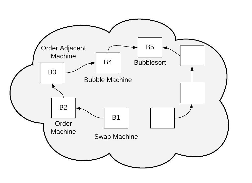
Figure 1. Approaching an algorithm (Bubblesort) via a sequence of transition systems (machines). The diagram shows two of the many possible design pathways.

By bringing in transition systems, we bring in an alternative notational and reasoning framework that is abstract, precise and compact. The framework allows the expression of mental models that align closer to the problem and the high-level operations rather than the implicit architectural model of a programming language (functions, while loops, etc.)

Students trace their programs to understand how their algorithm runs. Algodynamics connects it to a sequence of transitions. Because the elements of the trace operate on higher abstract actions, the cognitive load on the student is reduced.

At each stage in the process leading to the construction of the algorithm, we have a complete, interactive system that the student can play with, reason about and develop insight about the problem and the solution and explore other solutions and problems in the vicinity. This approach encourages creative experimentation (the highest level of Bloom’s taxonomy). In the programming part of the lab, the student is simply coding, in a systematic manner, the transition systems she has already understood.

In the rest of the paper, we review the literature on the difficulties of teaching and learning algorithms through programming(Section 2) and then include a short self-contained, introduction to transition systems and algodynamics (Section 3). We illustrate the algodynamics approach by exploring the Bubblesort algorithm (Section 4). Conclusions and future work are presented in Section 5.

2. Related Work

In this section, we briefly review the challenges students face that are related to problem solving, programming and algorithms.

Learning programming continues to be difficult, as evidenced by various studies on pass rates of introductory programming courses across various countries (Luxton-Reilly et al., 2019; Watson and Li, 2014; Bennedsen and Caspersen, 2007). The difficulties of novice programmers has been widely researched (Du Boulay, 1986; Spohrer and Soloway, 1986), including in a recent literature survey by Medeiros(Medeiros et al., 2019), who groups the difficulties of novice programmers into 4 categories: 1) problem formulation, 2) solution expression, 3) solution execution and evaluation, and 4) behavior.

Difficulties in problem formulation include problem solving, the abstract nature of programming, and algorithmic and logical reasoning. These resonate with Winslow’s discussion on novice vs. expert (Winslow, 1996): ”Experts tend to approach a program through its objects rather than control structures… experts use algorithms, rather than a specific syntax, abstracting from a particular language to the general concept.” Robins(Robins et al., 2003) lays out the novice vs. expert differences in great detail, citing several studies. He indicates ”the most important deficits relate to the underlying issues of problem solving, design, and expressing a solution/design as an actual program.” Fix (Fix et al., 1993) studies mental representation of programs by novices and experts and finds that the novice’s representation lacked the characteristics evidenced by the expert’s representation.

Program comprehension is another area cited as difficult for novices, as evidenced by their ability to trace the program and also explain it in English (Lister et al., 2004). Vainio (Vainio and Sajaniemi, 2007) studies the causes for poor tracing skills and describes 4 specific difficulties students face, including Inability to use external representations and inability to raise abstraction level. Lopez (Lopez et al., 2008) and Lister (Lister et al., 2009) also conclude that those who can’t trace well also can’t explain the code, and those who perform reasonably well at code writing have also acquired the ability to trace and explain.

Summarizing these observations, it seems clear that students need to acquire the following skills to become better at problem solving: 1) Abstraction and Modeling - ability to model the problem and think at an abstract level, using external representations as needed, 2) Program comprehension and tracing - ability to understand the program by tracing and explaining in English, and 3) Algorithmic reasoning - ability to reason logically rather than via program syntax and control structure.

An algorithm course in an undergraduate program is expected to address the above concerns. However, given the challenges above, it is important to first review the ways in which the teaching of algorithms is approached and to then propose pedagogical improvements that address the challenges above.

The concerns with the way algorithms are taught are not new. Levitin (Levitin, 2000) argued to reconsider the way we teach design and analysis of algorithms and incorporate more problem-solving, almost 20 years ago. While the constructivist approach has been espoused for teaching programming (Ben-Ari, 2001; Wulf, 2005) and constructionism (Harel and Papert, 1991) for experiential learning, we do not see evidence in the literature of knowledge construction approaches when teaching algorithms. Leading textbooks on algorithms (Cormen et al., 2009; Sahni and Horowitz, 1978; Skiena, 1998; Sedgewick, 1988) teach algorithms in a fait accompli manner - algorithms are presented in real code or pseudo-code, and the applicable strategy is pointed out (’divide and conquer’, ’backtracking’, ’greedy’, ’dynamic’, etc.). Computer Science Curricula 2013 (Joint Task Force on Computing Curricula and Society, 2013) approaches Algorithms and Complexity Body of Knowledge along similar lines. Use of code makes algorithm understanding hard for the same reason novice programmers find programming hard. Use of pseudo-code makes it only somewhat easier due to the lack of notational and semantic standards (Cutts et al., 2014). Such an approach to teaching doesn’t help the students in constructing their own knowledge about algorithm design.

A common and frequently discussed, approach in the literature for algorithm teaching is algorithm visualization (AV) (Shaffer et al., 2010; Alecha and Hermo, 2009; Alharbi et al., 2010; Vrachnos and Jimoyiannis, 2014; Amershi et al., 2008). While AV does offer better engagement and explainability, the outcomes and usage haven’t been significant enough to label it as an effective approach to teaching algorithms (Urquiza-Fuentes and Velázquez-Iturbide, 2009; Végh and Stoffová, 2017; Hundhausen et al., 2002). One of the challenges could be the limited role of interactivity in these visualizations. While there is evidence that adding interactivity to visualizations can positively impact understanding, (Wang et al., 2011; Patwardhan and Murthy, 2015), most of the algorithm visualizations available today lack interactivity.

An additional impediment that makes it hard harness interactivity and create game-like environments for algorithm teaching is that algorithms are inherently automatic and non-interactive.

We believe that an effective approach to teaching algorithms needs to focus on answering these questions: 1) How do we enable students to create abstract mental representations of algorithms? 2) How do we help students trace better and reason about the program? and 3) How do we let the students interact with the algorithm infrastructure and learn the principles of algorithm design through such interactions?

In his 1971 seminal paper (Wirth, 2001), Niklaus Wirth says: ”Clearly, programming courses should teach methods of design and construction, and the selected examples should be such that a gradual development can be nicely demonstrated.

In this paper, we take inspiration from the approach Wirth suggests for programming and apply it towards the design and construction of algorithms. The method we employ is interactive transition systems. The gradual development is demonstrated by the sequence of transition systems, each addressing a design concern and deciding on a data representation or control strategy. This way, students understand the nature of the algorithm and also engage with it sufficiently to develop their own understanding.

3. Transition Systems and the Algodynamics Approach

A transition system is a model to understand how quantities of interest change when subjected to outside forces called inputs or actions. The set of all possible values of the tuple of quantities constitute the state space of the system. Dynamics studies how the state changes when subjected to a series of actions over time. Algodynamics models algorithms as transition systems and studies their dynamics. In the algodynamics approach, finding a solution to a computation problem reduces to finding a sequence of the actions that steer a system from an initial state to its final state, the desired state.

Algodynamics explores the space between interactive systems and algorithms. In this space exist several transition systems, each presenting itself as an interactive laboratory that reveals some important aspect of the algorithm. The laboratory keeps the student engaged and encouraged to discover intereactively new ways to solve a problem. Because a transition system is interactive, the student can play with the system by choosing an action (akin to making a move in a game) and seeing its effect on the system’s state. What sequence of actions to apply is left to the student, and the student may devise her own strategy to choose these moves. From merely ‘observing’, or ‘tracing’ how an algorithm runs, the student now takes control and steers the system towards the solution. The student is now ‘learning by doing.’

The opposite of ‘interactive’ is ‘automated’. A transition system is said to be automated if there is only one action that can be performed on the state. Algorithms are automated systems. In the algodynamics approach, the student is introduced to a gradually developed series of increasingly less interactive transition systems which culminate in the algorithm. At each stage the student is trading interaction for automation. This allows the student to see the design of an algorithm emerge in an incremental manner.

3.1. Brief introduction to Transition Systems

Our definition of a transition system is one that has now become standard(Baier and Katoen, 2008; Tabuada, 2009; Belta et al., 2017). A transition system (TS) is a six-tuple $(X,X_{0},,U,\delta,Y,h)$ where $X$ is a set called the state space; $X_{0}$ is a subset of $X$ called the set of initial states; $U$ is a set called the set of actions; $\delta:X\times U\to 2^{X}$ is the transition function or dynamics; if $\delta(x,u)=x^{\prime}$ we write $x\stackrel{{\scriptstyle u}}{{\too}}x^{\prime}$, which is called a transition. $Y$ is a set called the view (or observation) space and $h:X\to Y$ is a map called the view map. A TS is automated if the action set is a singleton. The set of states, observation and actions could each be finite, infinite or continuous. A system is said to be deterministic if $|\delta(x,u)|\leq 1$ for all $x$ and $u$. For a deterministic system, whenever $x\stackrel{{\scriptstyle u}}{{\too}}x^{\prime}$, $x^{\prime}$ is unique. A state $x\in X$ is said to be terminating if $\delta(x,u)=\emptyset$ for all $u\in U$. A run is a sequence of linked transitions $x_{0}\stackrel{{\scriptstyle u_{1}}}{{\too}}x_{1}\stackrel{{\scriptstyle u_{2}}}{{\too}}x_{2}\cdots x_{n-1}\stackrel{{\scriptstyle u_{n}}}{{\too}}x_{n}.$ For a run as above the sequence of states $(x_{0},x_{1},\cdots,x_{n})$ is called a trajectory and the sequence of observations in the set $Y$, namely, $(h(x_{0}),h(x_{1}),\cdots,h(x_{n}))$      is called a trace. A TS is terminating if it has no infinitely long runs.

A TS is generally interactive. A user can choose an initial state $x_{0}$, and a sequence of actions $u_{1},u_{2},\cdots,u_{n}$ to construct a run and see what the trajectory looks like. She may like to choose actions that result in a specified trajectory. As remarked earlier a TS is said to be automated if there is only one action in $U$. In such a case the unique action is generally denoted by $next$ and there is no more any choice for the user in the construction of trajectories. The choice of an initial state determines the entire trajectory.

A computation problem is specified by choosing a view space $Y$, an initial subset $Y_{0}$ of $Y$, a final subset $Y_{\omega}$ of $Y$, and a map $f:X_{0}\to Y_{\omega}$ called the specification map. An interactive solution of a computation problem is a TS whose traces begin with some $y_{0}\in Y_{0}$ and end in $f(y_{0})\in Y_{\omega}$. If an interactive solution can be designed to be automated, terminating and deterministic, then the solution is called an algorithm.

In Algodynamics, we take the specification of a computation problem as stated above and try to construct tentatively an interactive solution with some wide and suitable choice of data types and actions to construct $X$ and $U$, followed by the full transition system. Then we progressively refine it to generate a sequence of interactive solutions that ends with an algorithm.

4. Illustrating the Algodynamics approach with Bubblesort

Algodynamics approach

We apply the algodynamics approach to explore the specification of the sorting problem and the Bubblesort algorithm. Our concern here is not Bubblesort’s efficiency (which is poor), nor its persistent use in algorithm pedagogy despite its many shortcomings(Astrachan, 2003), but its mechanics, which is simple, but not trivial.

The sorting problem may be specified as building an algorithmic system with initial observation $a^{0}$, an $n$-sized array of numbers to be sorted, and in whose terminal state, we observe $\id{sort}(a^{0})$, its sorted permutation. The goal is to build an algorithmic transition system for Bubblesort and implement it as a program.

4.1. A sequence of transition systems for Bubblesort

We suggest a sequence of five transition systems $B_{1}$ to $B_{5}$ to explore the design of Bubblesort. The sequence is but one of many possible trajectories in the design space that contains Bubblesort. Each system in the sequence $B_{1}$ to $B_{5}$ highlights a key decision in the design of Bubblesort. We present sample runs, and briefly note the key properties of the system. We include screenshots of online experiments for some of the systems. A full exposition should include mathematical arguments of correctness. We elide them here in the interest of brevity.

State variables and Notation: We use $a$ to denote the array state variable. The size of $a$ is assumed to be $n$ and element indexing is zero-based. In addition, we assume array index variables $0\leq i<j<n$ and $0\leq b\leq n$ which appear as part of the state vector in specific transition systems.

4.1.1. Transition System $B_{1}$: “Swap Machine”

$B_{1}$

Bubblesort rests on a key primitive: transposing or swapping elements in an array. The first system $B_{1}$ is designed around this idea. We assume $\id{swap}(a,i,j)$ denotes the result of swapping $a_{i}$ with $a_{j}$ in $a$. The state vector of $B_{1}$ consists of an array $a$. An action in $B_{1}$ is of the form ${\sf swap}(i,j)$, where $0\leq i<{j}<{n}$. The dynamics of $B_{1}$ is captured by the transition relation $a\ \xto{{\sf swap}(i,j)}{B_{1}}\ a^{\prime}\qquad\mbox{iff }a^{\prime}=\id{swap}(a,i,j)$.

$B_{1}$ runs

Here are example runs in $B_{1}$ starting with the array $[8,6,7,4]$. The underlines identify elements being swapped.

(1) $$[\underline{8},6,7,\underline{4}]\ \xto{{\sf swap}(0,3)}{B_{1}}\ [4,6,7,8]$$

(2) $$[8,\underline{6},\underline{7},4]\ \xto{{\sf swap}(1,2)}{B_{1}}\ [\underline{8},7,6,\underline{4}]\ \xto{{\sf swap}(0,3)}{B_{1}}\ [4,7,6,8]$$

Virtual Lab experiment

The runs may be easily created with paper and pencil by the student and on the blackboard by the teacher. In addition, the student may create and explore these interactively through a virtual experiment implementing this system. (See Figure 2.)

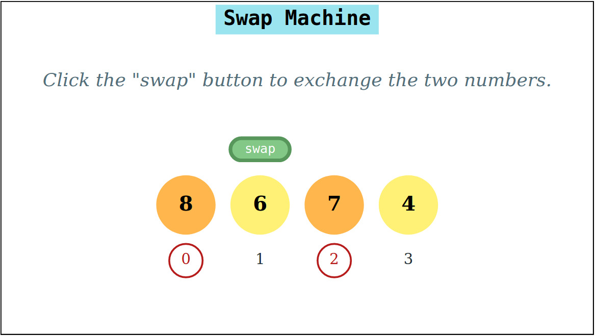
Figure 2. Online experiment based on transition system $B_{1}$ showing the swapping of elements

Exploring $B_{1}$’s capability to sort

Note that $B_{1}$ is interactive, deterministic and non-terminating. We are free to swap any two elements. This can sometimes, result in a very short run to sort an array (Run 1). The freedom also makes $B_{1}$ versatile. We can now use $B_{1}$ to not just sort, but also reverse a sequence (Run 2). With some practice, the student could conjecture that $B_{1}$ may be used to obtain any permutation of the array. The more inquisitive student may want to know why $B_{1}$ ‘works’ for sorting. The more mathematically oriented student may be encouraged to explore how this relates to the theory of permutation groups(Fraleigh, 2003).

4.1.2. Transition system $B_{2}$: “Order Machine”

$B_{2}$ defn

$B_{1}$ allows too much freedom and lacks direction. Playing with $B_{1}$, the student might realise that sorting can be done by swapping only those elements that are out of order (an operation we call ‘ordering’). The system $B_{2}$ captures this insight.

$B_{2}$ actions

The transition system $B_{2}$ has the array $a$ as its sole state variable. There is only one type of action in $B_{2}$: ${\sf order}(i,j)$, where, again $0\leq i<j<n$. The transition relation is $a\xto{{\sf order}(i,j)}{B_{2}}a^{\prime}$ iff $a_{i}>a_{j}\qquad\text{ and }a^{\prime}=\id{swap}(a,i,j)$.

Conjecture correctness

Interacting with the virtual experiment implementing $B_{2}$ should help the student conjecture that every run in $B_{2}$ terminates and the terminal state always is a sorted array. Of course, the mathematically inclined student may wish to prove this property.

4.1.3. Transition System $B_{3}$: “Order Adjacent machine”

$B_{3}$ definition

How do we choose indices for ordering? The simplest strategy picks adjacent elements. The transition system $B_{3}$ incorporates this choice. Therefore, $B_{3}$ has as its state variable the array $a$ and single type of action ${\sf adj}(i)$ where $0\leq i<n-1$. Its dynamics is described by the transitions in $B_{2}$: $a\ \xto{{\sf adj}(i)}{B_{3}}\ a^{\prime}$ iff $a\xto{{\sf order}(i,i+1)}{B_{2}}a^{\prime}$.

4.1.4. Transition System $B_{4}$: “Bubble” Machine

$B_{4}$ definition

$B_{3}$ still leaves undecided the strategy for selecting the next action. This problem is addressed by the system $B_{4}$, which adopts a simple, linear traversal strategy to automatically locate the next index. Note that now the choice of which index to consider for swapping adjacent elements is no longer available. It is automated via an index variable $i$ in $B_{4}$. $i$, initialised to $0$ is maintained as part of $B_{4}^{\prime}$s state, along with the sequence $a$.

${\sf inc}$ action in $B_{4}$

To achieve the linear incremental strategy, $B_{4}$ comes equipped with an action ${\sf inc}$. ${\sf inc}$ orders the adjacent elements at $i$ and $i+1$ and then automatically increments $i$. A sequence of ${\sf inc}$ actions sweep the array $a$ starting from $i=0$.

${\sf reset}$

A single sweep of the array is insufficient for sorting. Therefore, the student is given the option of resetting the index any time. A reset action heralds the beginning of a new sweep cycle. This is accomplished by the ${\sf reset}$ action:

Transition relation

For someone interested in observing only the array variable in $B_{4}$, the view function $h_{B_{4}}$ is just $h_{B_{4}}(a,i)=a$. The transitions for $B_{4}$ are: $(a,i)\xto{{\sf reset}}{B_{4}}(a,0)$, $(a,i)\xto{{\sf inc}}{B_{4}}(a,i+1)$ iff $i<n-1$ and $a_{i}\leq a_{i+1}$, and $(a,i)\xto{{\sf inc}}{B_{4}}(a^{\prime},i+1)$ iff $i<n-1$ and $a\xto{{\sf adj}(i)}{B_{3}}a^{\prime}$.

Conjecturing the bubbling of the maximum element

Playing with $B_{4}$ by tracing out a few runs, an observant student may notice the following phenomenon: the index $i$ carries along with it the maximum element in the array swept so far. The largest element ‘bubbles its’ way towards the right end of the array.

$B_{4}$ terminiation

However, the bubbling may be interrupted by a ${\sf reset}$ at any step. Furthermore, the reset could be invoked infinitely often. $B_{4}$ is thus no longer a terminating system.

4.1.5. Transition System $B_{5}$: “Bubblesort” machine

A student could discover that repeated sweeps of the $B_{4}$ machine can be used to arrange the maximum element of an array at position $n-1$, the next maximum at position $n-2$, and so on. This divides the array at any step into an unsorted part followed by a sorted part. Whenever the sweep index $i$ reaches the boundary between the two parts, a reset could be triggered. The system $B_{5}$ implements this strategy for resetting. The state vector of $B_{5}$ now includes an additional boundary variable $b$, that ranges from $0$ to $n$. A boundary value of $k$ means that (a) all elements $a_{k}$ to $a_{n-1}$ are sorted and (b) $a_{k}$ is greater than or equal to all elements $a_{0}$ to $a_{k-1}$.

With this insight, it is now possible to define the dynamics of $B_{5}$. The state vector $(a,i,b)$ is initialised to $(a^{0},0,n)$. The sweep index $i$ varies from $0$ to $b-1$. At each step, the sweep index $i$ is incremented, until it reaches $b-1$. After that $i$ is reset to $0$. Simultaneously, the boundary index $b$ is decremented. The system terminates when $b$ is less than or or equal to 1. $B_{5}$ has only one action ${\sf next}$. making it an automated system. The observable of $B_{5}$ is the array $a$. The dynamics of $B_{5}$ is defined below:

$$(a,i,b) \xto{{\sf next}}{B_{5}}\ (a^{\prime},i^{\prime},b) \text{iff }i<b-1\ \text{and }(a,i)\ \xto{{\sf inc}}{B_{4}}\ (a^{\prime},i^{\prime})$$

$$(a,i,b) \xto{{\sf next}}{B_{5}}(a^{\prime},i^{\prime},b-1) \text{iff }\ i=b-1\text{ and}\ (a,i)\ \xto{{\sf reset}}{B_{4}}(a^{\prime},i^{\prime})$$

An interactive experiment for $B_{5}$ allows the student to step through the bubblesort algorithm. A screenshot of the algorithm in progress is shown in Figure 3.

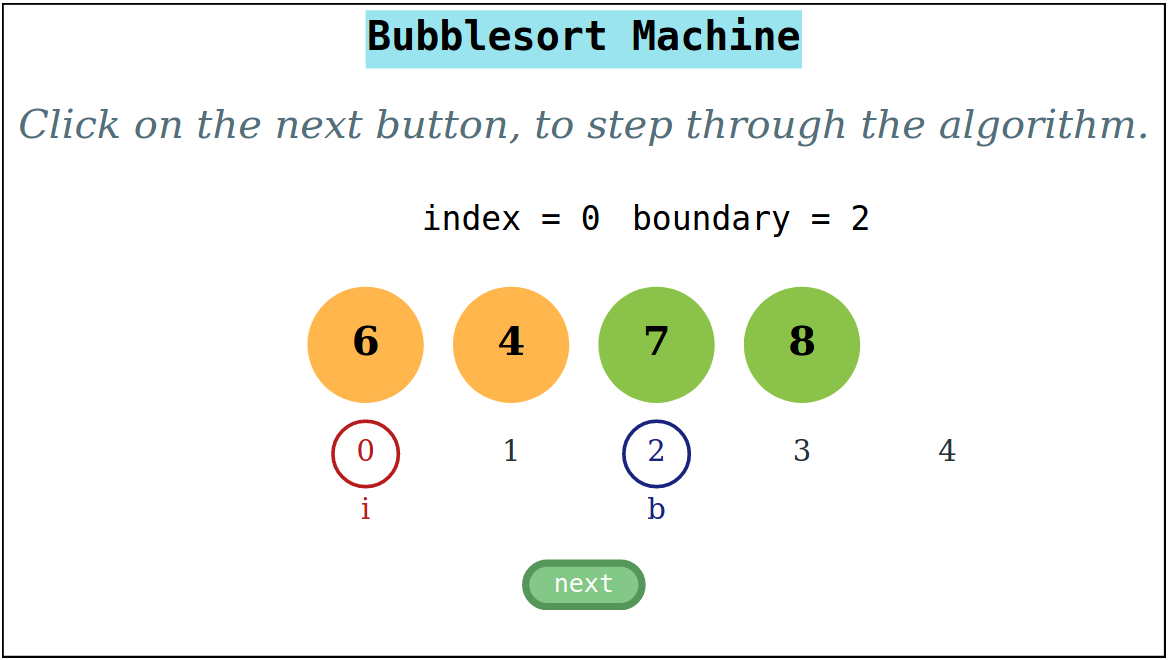
Figure 3. Screenshot of the Bubblesort algorithm (system $B_{5}$) displaying the values of array, index and boundary state variables during a sorting run.

Termination of $B_{5}$

Whenever $i$ reaches $b-1$, it is automatically reset, $b$ is decremented and as a result, the sorted segmented of the array grows by one. A formal correctness proof uses induction on the transition systems is not difficult, but omitted.

Table 1 compares the runs amongst the five transition systems $B_{1}$ to $B_{5}$ on the input array $[8,7,6,4]$. It is now a simple exercise for the student to improve the Bubblesort algorithm by incorporating a done? boolean state variable that terminates the algorithm as soon as there is a sweep with no swaps.

Table 1. The sorting of $[8,6,7,4]$ witnessed by runs in the various transition systems $B_{1}$ to $B_{5}$.. The boundary variable $b$ is part of only $B_{5}$’s state. The index variable $i$ (underlined) is part of only $B_{5}$’s and $B_{4}$’s state.

State	B${}_{\text{5}}$	B${}_{\text{4}}$	B${}_{\text{3}}$	B${}_{\text{2}}$	B${}_{\text{1}}$
$a$, $i$, $b$
$[\underline{8},6,7,4],0,4$	${\sf next}$	${\sf inc}$	${\sf adj}(0)$	${\sf order}(0,1)$	${\sf swap}(0,1)$
$[6,\underline{8},7,4],1,4$	${\sf next}$	${\sf inc}$	${\sf adj}(1)$	${\sf order}(1,2)$	${\sf swap}(1,2)$
$[6,7,\underline{8},4],2,4$	${\sf next}$	${\sf inc}$	${\sf adj}(2)$	${\sf order}(2,3)$	${\sf swap}(2,3)$
$[6,7,4,\underline{8}],3,4$	${\sf next}$	${\sf reset}$
$[\underline{6},7,4,8],0,3$	${\sf next}$	${\sf inc}$
$[6,\underline{7},4,8],1,3$	${\sf next}$	${\sf inc}$	${\sf adj}(1)$	${\sf order}(1,2)$	${\sf swap}(1,2)$
$[6,4,\underline{7},8],2,3$	${\sf next}$	${\sf reset}$
$[\underline{6},4,7,8],0,2$	${\sf next}$	${\sf inc}$	${\sf adj}(0)$	${\sf order}(0,1)$	${\sf swap}(0,1)$
$[4,\underline{6},7,8],1,2$	${\sf next}$	${\sf reset}$
$[\underline{4},6,7,8],0,1$

4.2. Coding the transition systems into a program

The process of translation consists of systematically coding the actions of each transition system. Each action maps to a function whose arguments consist of the state variables. The final transition system $B_{5}$ contains a single while loop along with a termination condition. A translation to Python code is show below: language=Python,label= ,caption= ,captionpos=b,numbers=none, basicstyle=small [language=Python, basicstyle=]bs-2col-no-comments.py

Prototype implementations of the five transitions systems suggested in this paper are available online(Authors, 2020).

5. Conclusions and Future work

We have introduced the algodynamics approach to teaching and designing of algorithms. We have illustrated the approach using Bubblesort. We have applied this approach on other sorting and searching algorithms, algorithms on trees, recursion and also concurrent algorithms. These will be reported elsewhere.

For the student, the algodynamics approach shows a clear way to think about the algorithm, in an interactive way. It encourages the teachers to construct their own pathways of transition systems to explain the design of an algorithm.

Field level trials (with suitably designed teaching kits), both for teachers and students are essential to test the efficacy of this approach and remain to be done. Incorporating the algodynamics approach in the syllabi of the algorithms course will require the introduction of transition systems earlier in the curriculum and integrating it with the course on automata theory. How this is to be done remains to be explored.

References

- (1)
- Alecha and Hermo (2009) Mikel Alecha and Montserrat Hermo. 2009. A Learning Algorithm for Deterministic Finite Automata using JFLAP. Electronic Notes in Theoretical Computer Science 248 (Aug. 2009), 47–56. https://doi.org/10.1016/j.entcs.2009.07.058
- Alharbi et al. (2010) Ali Alharbi, Frans Henskens, and Michael Hannaford. 2010. Integrated Standard Environment for the Teaching and Learning of Operating Systems Algorithms Using Visualizations. In 2010 Fifth International Multi-conference on Computing in the Global Information Technology. IEEE, Valencia, Spain, 205–208. https://doi.org/10.1109/ICCGI.2010.12
- Amershi et al. (2008) Saleema Amershi, Giuseppe Carenini, Cristina Conati, Alan K. Mackworth, and David Poole. 2008. Pedagogy and usability in interactive algorithm visualizations: Designing and evaluating CIspace. Interacting with Computers 20, 1 (Jan. 2008), 64–96. https://doi.org/10.1016/j.intcom.2007.08.003
- Astrachan (2003) Owen Astrachan. 2003. Bubble Sort: An Archaeological Algorithmic Analysis. SIGCSE Bull. 35, 1 (Jan. 2003), 1–5. https://doi.org/10.1145/792548.611918
- Authors (2020) Authors. 2020. Bubblesort Demo. https://vlab-exp.github.io/bubblesort.html
- Baier and Katoen (2008) Christel Baier and Joost-Pieter Katoen. 2008. Principles of Model Checking. MIT Press.
- Bellamy (1994) Rachel K. E. Bellamy. 1994. What Does Pseudo-Code Do? A Psychological Analysis of the Use of Pseudo-Code by Experienced Programmers. Hum.-Comput. Interact. 9, 3 (June 1994), 225–246. https://doi.org/10.1207/s15327051hci0902_3
- Belta et al. (2017) Calin Belta, Boyan Yordanov, and Ebru Aydin Gol. 2017. Formal Methods for Discrete-Time Dynamical Systems. Springer.
- Ben-Ari (2001) Mordechai Ben-Ari. 2001. Constructivism in computer science education. Journal of Computers in Mathematics and Science Teaching 20, 1 (2001), 45–73.
- Bennedsen and Caspersen (2007) Jens Bennedsen and Michael E Caspersen. 2007. Failure rates in introductory programming. AcM SIGcSE Bulletin 39, 2 (2007), 32–36.
- Blasco-Arcas et al. (2013) Lorena Blasco-Arcas, Isabel Buil, Blanca Hernández-Ortega, and F Javier Sese. 2013. Using clickers in class. The role of interactivity, active collaborative learning and engagement in learning performance. Computers & Education 62 (2013), 102–110.
- Cormen et al. (2009) Thomas H Cormen, Charles E Leiserson, Ronald L Rivest, and Clifford Stein. 2009. Introduction to algorithms. MIT press.
- Cutts et al. (2014) Quintin Cutts, Richard Connor, Greg Michaelson, and Peter Donaldson. 2014. Code or Not Code: Separating Formal and Natural Language in CS Education. In Proceedings of the 9th Workshop in Primary and Secondary Computing Education (WiPSCE ’14). Association for Computing Machinery, New York, NY, USA, 20–28. https://doi.org/10.1145/2670757.2670780
- Denning (2017) Peter J. Denning. 2017. Remaining Trouble Spots with Computational Thinking. Commun. ACM 60, 6 (May 2017), 33–39. https://doi.org/10.1145/2998438
- Du Boulay (1986) Benedict Du Boulay. 1986. Some Difficulties of Learning to Program. Journal of Educational Computing Research 2, 1 (Feb. 1986), 57–73. https://doi.org/10.2190/3LFX-9RRF-67T8-UVK9
- Fix et al. (1993) Vikki Fix, Susan Wiedenbeck, and Jean Scholtz. 1993. Mental representations of programs by novices and experts. In Proceedings of the SIGCHI conference on Human factors in computing systems - CHI ’93. ACM Press, Amsterdam, The Netherlands, 74–79. https://doi.org/10.1145/169059.169088
- Fraleigh (2003) J B Fraleigh. 2003. A First Course in Abstract Algebra (3rd ed.). Addison-Wesley.
- Guzdial et al. (2019) Mark Guzdial, Shriram Krishnamurthi, Juha Sorva, and Jan Vahrenhold. 2019. Notional Machines and Programming Language Semantics in Education (Dagstuhl Seminar 19281). Schloss Dagstuhl-Leibniz-Zentrum fuer Informatik.
- Halasz and Moran (1983) Frank G Halasz and Thomas P Moran. 1983. Mental models and problem solving in using a calculator. In Proceedings of the SIGCHI conference on Human Factors in Computing Systems. ACM, 212–216.
- Harel and Papert (1991) Idit Ed Harel and Seymour Ed Papert. 1991. Constructionism. Ablex Publishing.
- Hundhausen et al. (2002) Christopher D. Hundhausen, Sarah A. Douglas, and John T. Stasko. 2002. A Meta-Study of Algorithm Visualization Effectiveness. Journal of Visual Languages & Computing 13, 3 (June 2002), 259–290. https://doi.org/10.1006/jvlc.2002.0237
- Impagliazzo et al. (2003) John Impagliazzo, Robert Sloan, Andrew McGettrick, and Pradip K. Srimani. 2003. Computer Engineering Computing Curricula. SIGCSE Bull. 35, 1 (Jan. 2003), 355–356. https://doi.org/10.1145/792548.611915
- Joint Task Force on Computing Curricula and Society (2013) Association for Computing Machinery (ACM) Joint Task Force on Computing Curricula and IEEE Computer Society. 2013. Computer Science Curricula 2013: Curriculum Guidelines for Undergraduate Degree Programs in Computer Science. Association for Computing Machinery, New York, NY, USA.
- Lee and Seshia (2015) Edward A. Lee and Sanjit A. Seshia. 2015. Introduction to Embedded Systems, A Cyber-Physical Systems Approach, Second Edition. http://LeeSeshia.org. ISBN 978-1-312-42740-2.
- Levitin (2000) Anany Levitin. 2000. Design and analysis of algorithms reconsidered. ACM SIGCSE Bulletin 32, 1 (2000), 16–20.
- Lister et al. (2004) Raymond Lister, Elizabeth S Adams, Sue Fitzgerald, William Fone, John Hamer, Morten Lindholm, Robert McCartney, Jan Erik Moström, Kate Sanders, Otto Seppälä, et al. 2004. A multi-national study of reading and tracing skills in novice programmers. 36, 4 (2004), 119–150.
- Lister et al. (2009) Raymond Lister, Colin Fidge, and Donna Teague. 2009. Further evidence of a relationship between explaining, tracing and writing skills in introductory programming. Acm sigcse bulletin 41, 3 (2009), 161–165.
- Lopez et al. (2008) Mike Lopez, Jacqueline Whalley, Phil Robbins, and Raymond Lister. 2008. Relationships between reading, tracing and writing skills in introductory programming. In Proceeding of the fourth international workshop on Computing education research - ICER ’08. ACM Press, Sydney, Australia, 101–112. https://doi.org/10.1145/1404520.1404531
- Luxton-Reilly et al. (2019) Andrew Luxton-Reilly, Vangel V Ajanovski, Eric Fouh, Christabel Gonsalvez, Juho Leinonen, Jack Parkinson, Matthew Poole, and Neena Thota. 2019. Pass Rates in Introductory Programming and in other STEM Disciplines. (2019), 53–71.
- Medeiros et al. (2019) Rodrigo Pessoa Medeiros, Geber Lisboa Ramalho, and Taciana Pontual Falcao. 2019. A Systematic Literature Review on Teaching and Learning Introductory Programming in Higher Education. IEEE Transactions on Education 62, 2 (May 2019), 77–90. https://doi.org/10.1109/TE.2018.2864133
- on Computing Curricula (2015) The Joint Task Force on Computing Curricula. 2015. Curriculum Guidelines for Undergraduate Degree Programs in Software Engineering. Technical Report. New York, NY, USA.
- Patwardhan and Murthy (2015) Mrinal Patwardhan and Sahana Murthy. 2015. When does higher degree of interaction lead to higher learning in visualizations? Exploring the role of ‘Interactivity Enriching Features’. Computers & Education 82 (March 2015), 292–305. https://doi.org/10.1016/j.compedu.2014.11.018
- Robins et al. (2003) Anthony Robins, Janet Rountree, and Nathan Rountree. 2003. Learning and Teaching Programming: A Review and Discussion. Computer Science Education 13, 2 (June 2003), 137–172. https://doi.org/10.1076/csed.13.2.137.14200
- Roussou (2004) Maria Roussou. 2004. Learning by Doing and Learning through Play: An Exploration of Interactivity in Virtual Environments for Children. Comput. Entertain. 2, 1 (Jan. 2004), 10. https://doi.org/10.1145/973801.973818
- Sahni and Horowitz (1978) Sartaj Sahni and Ellis Horowitz. 1978. Fundamentals of computer algorithms. Computer Science Press.
- Sedgewick (1988) Robert Sedgewick. 1988. Algorithms. Pearson Education.
- Shaffer et al. (2010) Clifforda Shaffer, Matthew L. Cooper, Alexander Joel D. Alon, Monika Akbar, Michael Stewart, Sean Ponce, and Stephen H. Edwards. 2010. Algorithm Visualization: The State of the Field. ACM Transactions on Computing Education 10, 3 (Aug. 2010), 1–22. https://doi.org/10.1145/1821996.1821997
- Skiena (1998) Steven S Skiena. 1998. The algorithm design manual: Text. Vol. 1. Springer Science & Business Media.
- Sorva (2013) Juha Sorva. 2013. Notional Machines and Introductory Programming Education. ACM Trans. Comput. Educ. 13, 2, Article Article 8 (July 2013), 31 pages. https://doi.org/10.1145/2483710.2483713
- Spohrer and Soloway (1986) James C. Spohrer and Elliot Soloway. 1986. Novice mistakes: are the folk wisdoms correct? Commun. ACM 29, 7 (July 1986), 624–632. https://doi.org/10.1145/6138.6145
- Tabuada (2009) Paulo Tabuada. 2009. Verification and Control of Hybrid Systems: A Symbolic Approach. Springer.
- Urquiza-Fuentes and Velázquez-Iturbide (2009) Jaime Urquiza-Fuentes and J. Ángel Velázquez-Iturbide. 2009. A Survey of Successful Evaluations of Program Visualization and Algorithm Animation Systems. ACM Transactions on Computing Education 9, 2 (June 2009), 1–21. https://doi.org/10.1145/1538234.1538236
- Vainio and Sajaniemi (2007) Vesa Vainio and Jorma Sajaniemi. 2007. Factors in novice programmers’ poor tracing skills. 39, 3 (2007), 236–240.
- Vrachnos and Jimoyiannis (2014) Euripides Vrachnos and Athanassios Jimoyiannis. 2014. Design and Evaluation of a Web-based Dynamic Algorithm Visualization Environment for Novices. Procedia Computer Science 27 (2014), 229–239. https://doi.org/10.1016/j.procs.2014.02.026
- Végh and Stoffová (2017) Ladislav Végh and Veronika Stoffová. 2017. Algorithm Animations for Teaching and Learning the Main Ideas of Basic Sortings. Informatics in Education 16, 1 (March 2017), 121–140. https://doi.org/10.15388/infedu.2017.07
- Wang et al. (2011) Pei-Yu Wang, Brandon K. Vaughn, and Min Liu. 2011. The impact of animation interactivity on novices’ learning of introductory statistics. Computers & Education 56, 1 (Jan. 2011), 300–311. https://doi.org/10.1016/j.compedu.2010.07.011
- Watson and Li (2014) Christopher Watson and Frederick W.B. Li. 2014. Failure rates in introductory programming revisited. In Proceedings of the 2014 conference on Innovation & technology in computer science education - ITiCSE ’14. ACM Press, Uppsala, Sweden, 39–44. https://doi.org/10.1145/2591708.2591749
- Winslow (1996) Leon E. Winslow. 1996. Programming pedagogy—a psychological overview. ACM SIGCSE Bulletin 28, 3 (Sept. 1996), 17–22. https://doi.org/10.1145/234867.234872
- Wirth (2001) Niklaus Wirth. 2001. Program development by stepwise refinement. In Pioneers and Their Contributions to Software Engineering. Springer, 545–569.
- Wulf (2005) Tom Wulf. 2005. Constructivist Approaches for Teaching Computer Programming. In Proceedings of the 6th Conference on Information Technology Education (SIGITE ’05). Association for Computing Machinery, New York, NY, USA, 245–248. https://doi.org/10.1145/1095714.1095771