Statistical Inference for Maximin Effects:
Identifying Stable Associations across Multiple Studies

Integrative analysis of data from multiple sources is critical to making generalizable discoveries. Associations that are consistently observed across multiple source populations are more likely to be generalized to target populations with possible distributional shifts. In this paper, we model the heterogeneous multi-source data with multiple high-dimensional regressions and make inferences for the maximin effect (Meinshausen, Bühlmann, AoS, 43(4), 1801–1830). The maximin effect provides a measure of stable associations across multi-source data. A significant maximin effect indicates that a variable has commonly shared effects across multiple source populations, and these shared effects may be generalized to a broader set of target populations. There are challenges associated with inferring maximin effects because its point estimator can have a non-standard limiting distribution. We devise a novel sampling method to construct valid confidence intervals for maximin effects. The proposed confidence interval attains a parametric length. This sampling procedure and the related theoretical analysis are of independent interest for solving other non-standard inference problems. Using genetic data on yeast growth in multiple environments, we demonstrate that the genetic variants with significant maximin effects have generalizable effects under new environments.

KEYWORDS: Heterogeneous multi-source data; Distributionally robust optimization; Non-standard inference; High-dimensional Inference; Distributional shifts.

1 Introduction

1.1 Problem formulation

A vital component of contemporary medical and biological research is integrating multiple studies designed to study the same scientific question. Noteworthy examples include the integration of electronic health record (EHR) data from multiple hospitals (Singh et al., 2021; Rasmy et al., 2018) and genetic data collected from different subpopulations or environments (Keys et al., 2020; Sirugo et al., 2019; Kraft et al., 2009; Cai et al., 2021a). Synthesis of information from multiple sources enhances the model’s generalizability. For instance, the associations that are consistently observed across multiple source populations are more likely to be generalized to a wide range of target populations. However, the data heterogeneity creates challenges for prediction and inference. There is a pressing need to devise practical inference tools for extracting generalizable information from heterogeneous multi-source data.

We consider that we have access to $L$ independent training data sets $\{X^{(l)},Y^{(l)}\}_{1\leq l\leq L}$. For $1\leq l\leq L$, we assume that the data $\{X^{(l)}_{i},Y^{(l)}_{i}\}_{1\leq i\leq n_{l}}$ are i.i.d. generated following the high-dimensional model:

$$Y_{i}^{(l)}=[X^{(l)}_{i}]^{\intercal}b^{(l)}+\epsilon^{(l)}_{i}\quad\text{where}\quad\mathbf{E}(\epsilon^{(l)}_{i}\mid X^{(l)}_{i})=0,$$ (1)

with the outcome $Y^{(l)}_{i}\in\mathbb{R}$ and covariates $X^{(l)}_{i}\in\mathbb{R}^{p}$. To model the data heterogeneity, we allow $\{b^{(l)}\}_{1\leq l\leq L}$ and the distributions of $X^{(l)}_{i}$ and $\epsilon^{(l)}_{i}$ to vary with the group label $l$. Our goal is to leverage the multi-source data and construct a generalizable model for a target population. We use $\mathbb{Q}$ to denote the distribution of the target population. The target population may have a different covariate distribution $\mathbb{Q}_{X}$ and conditional outcome distribution $\mathbb{Q}_{Y|X}$ from source populations. We focus on the unlabelled target population: there are no outcome observations of the target population but only covariates $X^{\mathbb{Q}}_{i}\in\mathbb{R}^{p}$ for $1\leq i\leq N_{\mathbb{Q}}$. Such unlabelled settings frequently occur in EHR analysis (Humbert-Droz et al., 2022) or transfer learning (Zhuang et al., 2020; Pan and Yang, 2009), where the outcome labels of the target population are hard to obtain due to high costs. Due to possible distributional shifts of the unlabelled target population, identification of the true $\mathbb{Q}_{Y|X}$ is generally impossible in our framework.

This paper aims to make inferences about the covariate-shift maximin effect $\beta^{*}(\mathbb{Q})$ defined in the following equation (6). We generalize the definition in Meinshausen and Bühlmann (2015) by allowing for covariate shifts and define $\beta^{*}(\mathbb{Q})$ as the solution to a distributionally robust optimization problem. Particularly, we examine a wide range of target distributions that may contain the true $\mathbb{Q}$ and define $\beta^{*}(\mathbb{Q})$ as a linear model guaranteeing excellent predictive performance over this class of possible target distributions. According to Meinshausen and Bühlmann (2015), when the target population differs from the source populations, maximin effects provide superior predictive performance than the regression model constructed with the merged multi-source data.

The maximin effects not only guarantee robust predictive performance over a range of target distributions but also provide a measure of stable associations shared by regression vectors $\{b^{(l)}\}_{1\leq l\leq L}$ (Meinshausen and Bühlmann, 2015). Identifying variables with significant maximin effects is critical since their effects are more likely to be generalizable to new populations, even with possible distributional shifts. As shown in the following Proposition 1, $\beta^{*}(\mathbb{Q})$ is the convex combination of $\{b^{(l)}\}_{1\leq l\leq L}$ that has the minimum (weighted) distance to the origin; see the leftmost of Figure 1 for the illustration. The minimum distance ensures that $\beta^{*}(\mathbb{Q})$ summarizes stable associations shared across multiple source populations. As demonstrated on the rightmost of Figure 1, when a variable has heterogeneous effects scattered around zero across multiple studies, its maximin effect will shrink to zero; for essential predictors with commonly shared effects across multiple data sources, the maximin effect will capture the sign of the shared effects. Moreover, the maximin effect will not be dominated by the extreme effect, only showing up in a single study. In light of the above interpretation, a significant maximin effect indicates that a predictor has commonly shared effects across various populations.

Figure 1: Maximin effect (the red cross) for $p=2$. The left panel: $\beta^{*}(\mathbb{Q})$ is the convex combination of $\{b^{(l)}\}_{1\leq l\leq L}$ (black dots) having the smallest distance to the origin; the right panel: $\beta^{*}_{2}(\mathbb{Q})$ shrinks to zero when $\{b^{(l)}_{2}\}_{1\leq l\leq L}$ scatters around zero. The left and right figures duplicate Figure 1 in Bühlmann and Meinshausen (2015) and Figure 2 in Meinshausen and Bühlmann (2015), respectively.

Despite the importance of maximin effects, statistical inference methods for maximin effects are primarily lacking, including the construction of confidence interval (CI) and hypothesis testing. We demonstrate that the inference problem for the maximin effect is non-standard and devise a new sampling technique for solving these non-standard inference problems.

1.2 Our results and contribution

There are distinct challenges associated with inference for maximin effects, which occur both in low- and high-dimensional cases. Section 3 illustrates several challenging settings where the maximin effect estimator may have a non-standard limiting distribution. Consequently, we cannot construct CIs for the maximin effects directly based on the asymptotic normality. We propose a novel sampling procedure to construct CIs for the maximin effects in both low and high dimensions. The main novelty is to devise a sampling method to quantify the uncertainty associated with convex weight estimation. Our proposal relies on the following intuition: after carefully sampling a large number of weight vectors, there exists at least one resampled weight vector, almost recovering the true weight vector. We provide a rigorous statement of this property in Theorem 1. Our proposed sampling CI is shown to achieve the desired coverage level and attain the parametric length.

We conduct a large-scale simulation to evaluate the finite-sample performance. When the maximin effect estimator does not have a standard limiting distribution, the CIs based on asymptotic normality, subsampling, or the m-out-of-n bootstrap undercover, but our proposed CI achieves the desired coverage; see Section 7 and Section B in the supplement. In Section 8, we analyze genetic data on yeast colony growth under different growth media. The proposed inference method is compared with empirical risk minimization (ERM), which selects significant genetic variants by analyzing the merged training data. We compare our proposal and ERM by examining seven test media that were not used for training the models. The genetic variants having significant maximin effects are more generalizable to test growth media, while several genetic variants selected by ERM have no significant effects for any of these test media.

To summarize, the contributions of the current paper are two-folded,

1. We propose a novel sampling approach to make inferences for maximin effects. The sampling method is useful for addressing other non-standard inference problems.

2. We establish the sampling property in Theorem 1 and characterize the dependence of sampling accuracy on the resampling size. The theoretical argument is new and can be of independent interest for studying other sampling methods.

1.3 Related works

Distributionally robust optimization has been utilized in Gao et al. (2017); Sinha et al. (2017) to construct machine learning algorithms robust to the distributional shift between the training and test data. The main idea is to construct a prediction model that minimizes adversarial losses defined over a class of distributions near the source population. The current paper concerns the different settings where the prior knowledge of group information is present. When the group information is available, there has been an extensive study of the maximin effect and group distributionally robust models (Meinshausen and Bühlmann, 2015; Bühlmann and Meinshausen, 2015; Sagawa et al., 2019; Hu et al., 2018). These studies focused on estimation rather than the construction of CIs. One notable exception is that Rothenhäusler et al. (2016) focused on the low-dimensional setting and constructed CIs for the maximin effect based on the estimator’s asymptotic normality. However, we point out in Section 3 that the maximin effect estimators are not necessarily asymptotically normal in challenging settings. The simulation results presented in Section 7 demonstrate the undercoverage of CIs based on asymptotic normality.

Inference for the shared component of regression functions was considered under multiple high-dimensional linear models (Liu et al., 2020) and partially linear models (Zhao et al., 2016). In contrast, our proposed method does not require $\{b^{(l)}\}_{1\leq l\leq L}$ in (1) to share any similarity, and our model is more flexible in modeling the heterogeneity of multi-source data. Peters et al. (2016); Rothenhäusler et al. (2018); Arjovsky et al. (2019) constructed models satisfying certain invariance principles by analyzing the heterogeneous data.

Sampling methods have a long history in statistics, such as bootstrap (Efron, 1979; Efron and Tibshirani, 1994), subsampling (Politis et al., 1999), generalized fiducial inference (Zabell, 1992; Xie and Singh, 2013; Hannig et al., 2016) and repro sampling (Xie and Wang, 2022). In contrast, instead of directly sampling from the original data, we resample the estimator of the regression covariance matrix, which makes our proposed sampling method computationally efficient; see Remark 5. Inference in a single high-dimensional linear model was actively investigated in the recent decade (Zhang and Zhang, 2014; van de Geer et al., 2014; Javanmard and Montanari, 2014; Belloni et al., 2014; Chernozhukov et al., 2015; Farrell, 2015; Chernozhukov et al., 2018; Cai and Guo, 2017; Athey et al., 2018; Zhu and Bradic, 2018). Inference for maximin effects has the challenge of being a non-standard inference problem, which requires novel methods and theories; see more discussions in Section 3.

Notations. Define $n=\min_{1\leq l\leq L}\{n_{l}\}$. For $1\leq j\leq p,$ let $e_{j}$ denote the $j$-th Euclidean basis. We use $c$ and $C$ to denote generic positive constants that may vary from place to place. For positive sequences $a_{n}$ and $b_{n}$, $a_{n}\ll b_{n}$ if $\limsup_{n\rightarrow\infty}{a_{n}}/{b_{n}}=0$. The $\ell_{q}$ norm of a vector $x$ is defined as $\|x\|_{q}=\left(\sum_{l=1}^{p}|x_{l}|^{q}\right)^{\frac{1}{q}}$ for $q\geq 0$ with $\|x\|_{0}=\left|\{1\leq l\leq p:x_{l}\neq 0\}\right|$ and $\|x\|_{\infty}=\max_{1\leq l\leq p}|x_{l}|$. For a vector $x\in\mathbb{R}^{p}$, a matrix $X$, and a subset $S\subset[p]$, $x_{S}$ is the sub-vector of $x$ with indices in $S$ and $X_{S}$ denotes the sub-matrix of $X$ with row indices belonging to $S.$ For a symmetric matrix $A\in\mathbb{R}^{L\times L}$ with eigendecomposition $A=U\Lambda U^{\intercal}$, we use $\lambda_{\max}(A)$ and $\lambda_{\min}(A)$ to denote its maximum and minimum eigenvalues, respectively; define $A_{+}=U\Lambda_{+}U^{\intercal}$ with $(\Lambda_{+})_{l,l}=\max\{\Lambda_{l,l},0\}$ for $1\leq l\leq L.$ For a semi-positive matrix $A$, define $A^{1/2}=U\Lambda^{1/2}U^{\intercal}$ with $(\Lambda^{1/2})_{l,l}=\sqrt{\Lambda_{l,l}}$ for $1\leq l\leq L.$ We use $A^{-1/2}$ to denote the inverse of $A^{1/2}.$ We use ${\rm vecl}(A)\in\mathbb{R}^{L(L+1)/2}$ to denote the vector stacking the columns of the lower triangle part of $A$. We define the one-to-one index mapping $\pi$,

$$\pi(l,k)=\frac{(2L-k)(k-1)}{2}+l\quad\text{for}\quad(l,k)\in\mathcal{I}_{L}\coloneqq\{(l,k):1\leq k\leq l\leq L\},$$ (2)

which maps from the matrix index of the lower triangle part of $A$ to ${\rm vecl}(A).$ For $(l,k)\in\mathcal{I}_{L},$ we have $[{\rm vecl}(A)]_{\pi(l,k)}=A_{l,k}.$

2 Maximin Effects: Distributional Robustness and Identification

2.1 Multi-source data setup

We introduce the setting in the following and present the definition and identification of the covariate-shift maximin effect in Sections 2.2 and 2.3, respectively. We consider the training data $\{X^{(l)},Y^{(l)}\}_{1\leq l\leq L}$ collected from $L$ sources (e.g., $L$ healthcare centers). For $1\leq l\leq L$, let $\mathbb{P}^{(l)}_{X}$ denote the distribution of $X^{(l)}_{i}\in\mathbb{R}^{p}$ and $\mathbb{P}^{(l)}_{Y|X}$ denote the conditional distribution of the outcome $Y^{(l)}_{i}$ given $X^{(l)}_{i}.$ We write

$$X^{(l)}_{i}{\;\mathrel{\overset{\rm i.i.d.}{\scalebox{1.5}[1.0]{$\sim$}}}\;}\mathbb{P}^{(l)}_{X},\quad Y^{(l)}_{i}\mid X^{(l)}_{i}{\;\mathrel{\overset{\rm i.i.d.}{\scalebox{1.5}[1.0]{$\sim$}}}\;}\mathbb{P}^{(l)}_{Y|X}\quad\text{for}\quad 1\leq i\leq n_{l}.$$ (3)

Heterogeneity may exist when the multi-source data are collected for different subpopulations or under different environments. To model this, we allow $\{\mathbb{P}^{(l)}_{X},\mathbb{P}^{(l)}_{Y|X}\}_{1\leq l\leq L}$ to be different from each other. For the target population (e.g., a new healthcare center), we use $\mathbb{Q}_{X}$ and $\mathbb{Q}_{Y|X}$ to respectively denote the covariate and conditional outcome distribution and write

$$X^{\mathbb{Q}}_{i}{\;\mathrel{\overset{\rm i.i.d.}{\scalebox{1.5}[1.0]{$\sim$}}}\;}\mathbb{Q}_{X},\quad Y^{\mathbb{Q}}_{i}\mid X^{\mathbb{Q}}_{i}{\;\mathrel{\overset{\rm i.i.d.}{\scalebox{1.5}[1.0]{$\sim$}}}\;}\mathbb{Q}_{Y|X}\quad\text{for}\quad 1\leq i\leq N_{\mathbb{Q}}.$$ (4)

We use $\{X^{(l)}_{i}\}_{1\leq l\leq L}$ and $X^{\mathbb{Q}}_{i}$ to denote the measurement of the same set of covariates across different subpopulations or under different environments; $\{Y^{(l)}_{i}\}_{1\leq l\leq L}$ and $Y^{\mathbb{Q}}_{i}$ to denote the measurement of the same outcome variable across different subpopulations or under different environments. This paper allows for the co-existence of covariate shifts and posterior drifts between the source and target populations, where the covariate shift stands for the covariate distribution $\mathbb{Q}_{X}$ differing from any of $\{\mathbb{P}^{(l)}_{X}\}_{1\leq l\leq L}$ and the posterior drift stands for the conditional outcome distribution $\mathbb{Q}_{Y|X}$ differing from any of $\{\mathbb{P}^{(l)}_{Y|X}\}_{1\leq l\leq L}$.

We focus on the regime where the target population does not have outcome labels, that is, the covariates $\{X^{\mathbb{Q}}_{i}\}_{1\leq i\leq N_{\mathbb{Q}}}$ are observed, but the outcome labels $\{Y^{\mathbb{Q}}_{i}\}_{1\leq i\leq N_{\mathbb{Q}}}$ are missing. Such an unlabelled setting is common in EHR data analysis (Humbert-Droz et al., 2022) and transfer learning applications (Zhuang et al., 2020; Pan and Yang, 2009). For example, due to the high costs, a new hospital might not have the outcome labels.

2.2 Maximin effects: generalizability via distributionally robust optimization

When the target population does not have outcome observations and $\mathbb{Q}_{Y|X}$ is allowed to differ from any of $\{\mathbb{P}^{(l)}_{Y|X}\}_{1\leq l\leq L}$, $\mathbb{Q}_{Y|X}$ is in general not identifiable. Instead of making inferences for the true $\mathbb{Q}_{Y|X}$, we introduce in the following a new inference target, the covariate-shift maximin effect, as a solution to a distributionally robust optimization problem. We define the following class of joint distributions which might contain the true $\mathbb{Q}$,

$$\mathcal{C}(\mathbb{Q}_{X})\coloneqq\left\{\mathbb{T}=(\mathbb{Q}_{X},\mathbb{T}_{Y|X}):\mathbb{T}_{Y|X}=\sum_{l=1}^{L}q_{l}\cdot\mathbb{P}^{(l)}_{Y|X}\;\;\;\text{with}\;\;\;q\in\Delta^{L}\right\},$$ (5)

where $\Delta^{L}=\{q\in\mathbb{R}^{L}:\sum_{l=1}^{L}q_{l}=1,\min_{l}q_{l}\geq 0\}$ denotes the $L$-dimension simplex. In (5), the covariate distribution is fixed at $\mathbb{Q}_{X}$ since it is identifiable with the data $\{X^{\mathbb{Q}}_{i}\}_{1\leq i\leq N_{\mathbb{Q}}}$; however, since the $\mathbb{Q}_{Y|X}$ is not identifiable, we consider the conditional outcome distribution as any convex combination of $\{\mathbb{P}^{(l)}_{Y|X}\}_{1\leq l\leq L}$. When the true $\mathbb{Q}_{Y|X}$ lies in the convex combination of $\{\mathbb{P}^{(l)}_{Y|X}\}_{1\leq l\leq L},$ the distribution class $\mathcal{C}(\mathbb{Q}_{X})$ contains the true target population $\mathbb{Q}=\left(\mathbb{Q}_{X},\mathbb{Q}_{Y|X}\right).$

We now define the maximin effect as a model optimizing the worst-case reward associated with the distribution class $\mathcal{C}(\mathbb{Q}_{X})$. For a generic model $\beta\in\mathbb{R}^{p}$, the reward function $\mathbf{E}_{(X_{i},Y_{i})\sim\mathbb{T}}\left[Y_{i}^{2}-(Y_{i}-X_{i}^{\intercal}\beta)^{2}\right]$ measures the variance explained by $X_{i}^{\intercal}\beta$ when the test data $\{X_{i},Y_{i}\}$ are generated following the distribution $\mathbb{T}$. We define the worst-case reward of the model $\beta$ as $R_{\mathbb{Q}}(\beta)=\min_{\mathbb{T}\in\mathcal{C}(\mathbb{Q}_{X})}\mathbf{E}_{(X_{i},Y_{i})\sim\mathbb{T}}\left[Y_{i}^{2}-(Y_{i}-X_{i}^{\intercal}\beta)^{2}\right],$ which examines every population $\mathbb{T}$ belonging to $\mathcal{C}(\mathbb{Q}_{X}).$ The covariate-shift maximin effect $\beta^{*}(\mathbb{Q})$ is defined to optimize the worst-case reward,

$$\beta^{*}(\mathbb{Q}):=\operatorname*{arg\,max}_{\beta\in\mathbb{R}^{p}}R_{\mathbb{Q}}(\beta)\quad\text{with}\quad R_{\mathbb{Q}}(\beta)=\min_{\mathbb{T}\in\mathcal{C}(\mathbb{Q}_{X})}\mathbf{E}_{(X_{i},Y_{i})\sim\mathbb{T}}\left[Y_{i}^{2}-(Y_{i}-X_{i}^{\intercal}\beta)^{2}\right],$$ (6)

where $\mathcal{C}(\mathbb{Q}_{X})$ is defined in (5) and $\mathbf{E}_{(X_{i},Y_{i})\sim\mathbb{T}}$ denotes the expectation with respect to the distribution $\mathbb{T}$. The definition of $\beta^{*}(\mathbb{Q})$ can be interpreted from a two-side game perspective (Meinshausen and Bühlmann, 2015): we select a model $\beta$, and the counter agent searches over $\mathcal{C}(\mathbb{Q}_{X})$ and generates the most challenging target population for this $\beta$. $\beta^{*}(\mathbb{Q})$ guarantees the optimal prediction accuracy for such an adversarially generated target population.

The robust prediction model $\beta^{*}(\mathbb{Q})$ guarantees excellent predictive performance for a broad class of target populations belonging to $\mathcal{C}(\mathbb{Q}_{X}).$ This explains the generalizability of $\beta^{*}(\mathbb{Q})$ since it is not designed to optimize the predictive performance for a single target population but over many possible target populations. $\beta^{*}(\mathbb{Q})$ is typically different from the best linear approximation derived from the true $\mathbb{Q}_{Y|X},$ which is not identifiable under our framework.

The definition (6) falls into the general category of distributionally robust optimization (Sagawa et al., 2019; Hu et al., 2018; Rothenhäusler et al., 2018; Gao et al., 2017; Sinha et al., 2017; Jakobsen and Peters, 2022, e.g.), who proposed to achieve the distributional robustness by investigating the predictive performance for a class of target distributions. We have provided a distributional robustness interpretation of the maximin effect in Meinshausen and Bühlmann (2015) and generalized its definition by allowing for distributional shifts among $\mathbb{Q}_{X}$ and $\{\mathbb{P}^{(l)}_{X}\}_{1\leq l\leq L}$. When there is no covariate shift, let $\mathbb{P}_{X}$ denote the shared covariate distribution of the source and target populations. $\beta^{*}(\mathbb{Q})$ in (6) is equivalent to the maximin effect defined in Meinshausen and Bühlmann (2015). The maximin effect in (6) can be expressed as an equivalent minimax estimator $\beta^{*}(\mathbb{Q}):=\operatorname*{arg\,min}_{\beta\in\mathbb{R}^{p}}\max_{\mathbb{T}\in\mathcal{C}(\mathbb{Q}_{X})}\left\{\mathbf{E}_{\mathbb{T}}\ell(Y_{i},X_{i}^{\intercal}\beta)\right\}$ with $\ell(Y_{i},X_{i}^{\intercal}\beta)=(Y_{i}-X_{i}^{\intercal}\beta)^{2}-Y_{i}^{2}$, which is in the form of the group distributionally robust optimization (Sagawa et al., 2019; Hu et al., 2018).

The maximin or minimax optimizations have essential applications to minimax group fairness (Martinez et al., 2020; Diana et al., 2021) and the maximin projection (Shi et al., 2018). In the supplement, we provide more detailed discussions in Sections A.1 and A.2.

Remark 1.

A collection of transfer learning algorithms are designed to leverage the assumption $\mathbb{Q}_{Y|X}\approx\mathbb{P}^{(l)}_{Y|X}$ for some $1\leq l\leq L$ and estimate $\mathbb{Q}_{Y|X}$; see Liu et al. (2020); Zhao et al. (2016); Li et al. (2020); Tian and Feng (2021) for examples. In contrast, our framework does not impose such similarity conditions. Our goal is to construct a generalizable prediction model over a range of target populations instead of recovering the true $\mathbb{Q}_{Y|X}.$

2.3 Identification and interpretation of $\beta^{*}(\mathbb{Q})$

In the following, we present the identification of $\beta^{*}(\mathbb{Q})$ defined in (6) and emphasize that $\beta^{*}(\mathbb{Q})$ summarizes the stable associations shared by multi-source data. We focus on the multiple linear models as in (1) for the remaining of this paper. The linear models in (1) can be extended to handle non-linear conditional expectation if $X^{(l)}_{i}$ contains the basis transformation of the covariates. Under (1), we simplify the definition of $\beta^{*}(\mathbb{Q})$ in (6) as

$$\beta^{*}(\mathbb{Q})=\operatorname*{arg\,max}_{\beta\in\mathbb{R}^{p}}R_{\mathbb{Q}}(\beta)\quad\text{with}\quad R_{\mathbb{Q}}(\beta)=\min_{b\in\mathbb{B}}\left[2b^{\intercal}\Sigma^{\mathbb{Q}}\beta-\beta^{\intercal}\Sigma^{\mathbb{Q}}\beta\right],$$ (7)

where $\mathbb{B}=\{b\in\mathbb{R}^{p}:b=\sum_{l=1}^{L}q_{l}\cdot b^{(l)}\;\text{with}\;q\in\Delta^{L}\}$ and $\Sigma^{\mathbb{Q}}=\mathbf{E}X_{1}^{\mathbb{Q}}(X_{1}^{\mathbb{Q}})^{\intercal}.$

The following proposition shows how to identify the maximin effect $\beta^{*}(\mathbb{Q}).$

Proposition 1.

If the model (1) holds and $\lambda_{\min}(\Sigma^{\mathbb{Q}})>0$, $\beta^{*}(\mathbb{Q})$ defined in (6) is identified as

$$\beta^{*}(\mathbb{Q})=\sum_{l=1}^{L}[\gamma^{*}(\mathbb{Q})]_{l}b^{(l)}\quad\text{with}\quad\gamma^{*}(\mathbb{Q})\coloneqq\operatorname*{arg\,min}_{\gamma\in\Delta^{L}}\gamma^{\intercal}\Gamma^{\mathbb{Q}}\gamma$$ (8)

where $\Gamma_{lk}^{\mathbb{Q}}=(b^{(l)})^{\intercal}\Sigma^{\mathbb{Q}}b^{(k)}$ for $1\leq l,k\leq L$ and $\Delta^{L}=\{\gamma\in\mathbb{R}^{L}:\gamma_{j}\geq 0,\;\sum_{j=1}^{L}\gamma_{j}=1\}$ is the simplex over $\mathbb{R}^{L}$. Furthermore, $\max_{\beta\in\mathbb{R}^{p}}R_{\mathbb{Q}}(\beta)=[\beta^{*}(\mathbb{Q})]^{\intercal}\Sigma^{\mathbb{Q}}\beta^{*}(\mathbb{Q}).$

Proposition 1 provides an explicit way of computing $\beta^{*}(\mathbb{Q})$, which is a generalization of Theorem 1 in Meinshausen and Bühlmann (2015). For any $\gamma$, $\gamma^{\intercal}\Gamma^{\mathbb{Q}}\gamma=\mathbf{E}\left[(X^{\mathbb{Q}}_{i})^{\intercal}\sum_{l=1}^{L}{\gamma}_{l}b^{(l)}\right]^{2}$ represents the second-order moment of the predicted values $(X^{\mathbb{Q}}_{i})^{\intercal}\sum_{l=1}^{L}{\gamma}_{l}b^{(l)}$ evaluated on the target population. The optimal weight is defined to minimize this second-order moment. Geometrically speaking, $\beta^{*}(\mathbb{Q})$ represents the point on the convex hull of $\{b^{(l)}\}_{1\leq l\leq L}$ that is closest to the origin (Meinshausen and Bühlmann, 2015). This interpretation ensures that the maximin effect summarizes the stable associations shared by the heterogeneous regression vectors $\{b^{(l)}\}_{1\leq l\leq L}$. As illustrated in Figure 1, when $\{b_{j}^{(l)}\}_{1\leq l\leq L}$ have different signs across different sources, $\beta^{*}_{j}$ will shrink to zero due to the cancelation in (8). However, if $\{b_{j}^{(l)}\}_{1\leq l\leq L}$ share the same sign, the convex combination in (8) ensures that the maximin effect shares the same sign. When there is no confusion, we write $\Gamma^{\mathbb{Q}},\beta^{*}(\mathbb{Q}),\gamma^{*}(\mathbb{Q})$ as $\Gamma,\beta^{*},\gamma^{*}$, respectively.

It is important to conduct statistical inference for $w^{\intercal}\beta^{*}$ with $w$ denoting a pre-specified loading. With $w=e_{j}$, the test of $w^{\intercal}\beta^{*}=0$ is reduced to the maximin significance test $H_{0,j}:\beta^{*}_{j}=0$ for $1\leq j\leq p$, which is crucial for scientific discovery and robust prediction model construction. The maximin significance of the $j$-th covariate indicates that its effect is homogeneously positive or negative across multiple environments; moreover, it indicates that the $j$-th covariate is likely to have a similar effect for a new environment. The non-zero maximin effect also suggests that it can be helpful to include the $j$-th covariate in the prediction model for the target population. Additionally, with $w$ denoting a future covariate observation, statistical inference for $w^{\intercal}\beta^{*}$ is well motivated by constructing an optimal treatment regime with heterogeneous data (Shi et al., 2018). We provide more discussions in Section A.2 in the supplement.

Remark 2.

In the covariate shift setting, a collection of works (Tsuboi et al., 2009; Shimodaira, 2000; Sugiyama et al., 2007, e.g.) were focused on the misspecified conditional outcome models. In contrast, we focus on the correctly specified conditional outcome model (1). Consequently, the regression vectors $\{b^{(l)}\}_{1\leq l\leq L}$ do not change with the target population $\mathbb{Q}_{X}$. However, the maximin effect $\beta^{*}(\mathbb{Q})$ changes with the target population since the weight $\gamma^{*}(\mathbb{Q})$ is determined by the target covariate distribution $\mathbb{Q}_{X}$.

3 Statistical Inference Challenges: Non-regularity and Instability

In the following, we demonstrate the inference challenges for the maximin effect and will devise a novel sampling approach in Section 4 to address these challenges. The inference challenges arise from that estimators of $\gamma^{*}(\mathbb{Q})$ and $\beta^{*}(\mathbb{Q})$ may have a non-standard limiting distribution. To demonstrate the challenges, we consider the special case $L=2$ and obtain the solution of (8) as $\gamma^{*}(\mathbb{Q})=(\gamma^{*}_{1},1-\gamma^{*}_{1})^{\intercal}$ with

$$\gamma^{*}_{1}=\min\left\{\max\left\{\frac{\Gamma^{\mathbb{Q}}_{22}-\Gamma^{\mathbb{Q}}_{12}}{\Gamma^{\mathbb{Q}}_{11}+\Gamma^{\mathbb{Q}}_{22}-2\Gamma^{\mathbb{Q}}_{12}},0\right\},1\right\}.$$ (9)

We construct an approximately unbiased estimator $\widehat{\Gamma}^{\mathbb{Q}}$ for $\Gamma^{\mathbb{Q}}$ in the following equation (15) and then estimate $\gamma^{*}_{1}$ by $\widehat{\gamma}_{1}=\min\left\{\max\left\{\bar{\gamma}_{1},0\right\},1\right\}$ with $\bar{\gamma}_{1}=\frac{\widehat{\Gamma}^{\mathbb{Q}}_{22}-\widehat{\Gamma}^{\mathbb{Q}}_{12}}{\widehat{\Gamma}^{\mathbb{Q}}_{11}+\widehat{\Gamma}^{\mathbb{Q}}_{22}-2\widehat{\Gamma}^{\mathbb{Q}}_{12}}$.

We illustrate two challenging settings where $\widehat{\gamma}_{1}$ may not have a standard limiting distribution even if $\widehat{\Gamma}^{\mathbb{Q}}$ is asymptotically normal. The first is the non-regularity setting due to the boundary effect. The estimation error $\widehat{\gamma}_{1}-\gamma^{*}_{1}$ is decomposed as a mixture distribution, $\sqrt{n}(\bar{\gamma}_{1}-{\gamma}^{*}_{1})\cdot{\bf 1}\{0<\bar{\gamma}_{1}<1\}+(-\sqrt{n}{\gamma}^{*}_{1})\cdot{\bf 1}\{\bar{\gamma}_{1}\leq 0\}+\sqrt{n}(1-{\gamma}^{*}_{1})\cdot{\bf 1}\{\bar{\gamma}_{1}\geq 1\},$ where the last two terms appear due to the boundary constraint $0\leq\gamma^{*}_{1}\leq 1.$ It is well known that boundary constraints lead to estimators with non-standard limiting distributions; see Self and Liang (1987); Andrews (1999); Drton (2009) and the references therein. Similarly, the boundary effect leads to a non-standard or non-regular distribution for the corresponding maximin effect estimator. For non-regular settings due to the boundary effect, inference methods based on asymptotic normality or bootstrap fail to work (Andrews, 2000, e.g.).

The second challenge is instability, which occurs when some of $\{b^{(l)}\}_{1\leq l\leq L}$ are similar to each other. For $L=2,$ if $b^{(1)}\approx b^{(2)}$, then $\Gamma^{\mathbb{Q}}_{11}+\Gamma^{\mathbb{Q}}_{22}-2\Gamma^{\mathbb{Q}}_{12}$ in (9) is close to zero. It is hard to accurately estimate $\gamma^{*}_{1}$ since a small error in estimating $\Gamma^{\mathbb{Q}}_{11}+\Gamma^{\mathbb{Q}}_{22}-2\Gamma^{\mathbb{Q}}_{12}$ may lead to a large error of estimating $\gamma^{*}_{1}.$ In Section 7 and Section B in the supplement, we illustrate that CIs assuming the asymptotic normality and by $m$ out of $n$ bootstrap or subsampling fail to provide valid inference for the maximin effect in the presence of non-regularity or instability.

4 Sampling Inference Methods for Maximin Effects

We devise a novel sampling approach to make inference for $w^{\intercal}\beta^{*}$ with $w$ denoting the pre-specified loading vector. As an important example, $w^{\intercal}\beta^{*}$ becomes $\beta^{*}_{j}$ with $w=e_{j}.$ In Section 4.1, we construct the estimators $\{\widehat{w^{\intercal}b^{(l)}}\}_{1\leq l\leq L}$ and $\widehat{\Gamma}^{\mathbb{Q}}$ and employ Proposition 1 to construct the point estimator of $w^{\intercal}\beta^{*}$ as

$$\widehat{w^{\intercal}\beta^{*}}=\sum_{l=1}^{L}\widehat{\gamma}_{l}\cdot\widehat{w^{\intercal}b^{(l)}}\quad\text{with}\quad\widehat{\gamma}:=\arg\min_{\gamma\in\Delta^{L}}\gamma^{\intercal}\widehat{\Gamma}^{\mathbb{Q}}\gamma.$$ (10)

In Section 4.2, we propose a novel sampling method to quantify the uncertainty of $\widehat{w^{\intercal}\beta^{*}}$ defined in (10) and construct the CI for $w^{\intercal}\beta^{*}$.

4.1 Point estimation of $w^{\intercal}\beta^{*}$

The point estimator in (10) relies on good initial esitmators $\{\widehat{w^{\intercal}b^{(l)}}\}_{1\leq l\leq L}$ and $\widehat{\Gamma}^{\mathbb{Q}}.$ In the following, we consider both low- and high-dimensional settings and construct $\{\widehat{w^{\intercal}b^{(l)}}\}_{1\leq l\leq L}$ and $\widehat{\Gamma}^{\mathbb{Q}}$ satisfying

$$(\widehat{w^{\intercal}b^{(l)}}-w^{\intercal}b^{(l)})/{\sqrt{\widehat{\rm V}^{(l)}_{w}}}\overset{d}{\to}\mathcal{N}(0,1),\quad{\rm vecl}(\widehat{\Gamma}^{\mathbb{Q}}-\Gamma^{\mathbb{Q}})\stackrel{{\scriptstyle d}}{{\approx}}\mathcal{N}({\bf 0},\widehat{\bf V}),$$ (11)

where ${\widehat{\rm V}^{(l)}_{w}}$ and $\widehat{\bf V}$ denote the estimated covariance to be respectively specified in the following equations (14) and (16), ${\rm vecl}(\widehat{\Gamma}^{\mathbb{Q}}-\Gamma^{\mathbb{Q}})$ is the vector stacking the columns of the lower triangular part of the matrix $\widehat{\Gamma}^{\mathbb{Q}}-\Gamma^{\mathbb{Q}}$, $\overset{d}{\to}$ stands for convergence in distribution, and $\stackrel{{\scriptstyle d}}{{\approx}}$ stands for approximately equal in distribution.

4.1.1 Low-dimensional setting

We start with the low-dimensional setting and provide intuitions for the construction of $\widehat{w^{\intercal}b^{(l)}}$ and $\widehat{\Gamma}^{\mathbb{Q}}.$ For $1\leq l\leq L$, let $\widehat{b}^{(l)}_{\rm OLS}$ denote the OLS estimator computed based on $(X^{(l)},Y^{(l)}).$ We estimate $w^{\intercal}{b}^{(l)}$ and $\Gamma^{\mathbb{Q}}$ by plugging in the OLS and sample covariance matrix. Define

$$\widehat{w^{\intercal}b^{(l)}}=w^{\intercal}\widehat{b}^{(l)}_{\rm OLS}\quad\text{for}\quad 1\leq l\leq L$$

$$\widehat{\Gamma}^{\mathbb{Q}}_{l,k}=\left[\widehat{b}^{(l)}_{\rm OLS}\right]^{\intercal}\left(\frac{1}{N_{\mathbb{Q}}}\sum_{i=1}^{N_{\mathbb{Q}}}X^{\mathbb{Q}}_{i}[X^{\mathbb{Q}}_{i}]^{\intercal}\right)\widehat{b}^{(k)}_{\rm OLS}\quad\text{for}\quad 1\leq k\leq l\leq L.$$ (12)

The standard regression theory guarantees that these plug-in estimators satisfy (11) under regularity conditions, where ${\widehat{\rm V}^{(l)}_{w}}={\widehat{\sigma}_{l}^{2}}\cdot w^{\intercal}[(X^{(l)})^{\intercal}X^{(l)}]^{-1}w$ with $\widehat{\sigma}_{l}^{2}=\|Y^{(l)}-X^{(l)}\widehat{b}^{(l)}_{\rm OLS}\|_{2}^{2}/(n_{l}-p)$ and $\widehat{\bf V}$ is presented in the following Remark 3.

4.1.2 High-dimensional setting

In high dimensions, $\{b^{(l)}\}_{1\leq l\leq L}$ are estimated by penalized estimators. If we simply plug in the penalized estimators, it leads to biased estimators of $w^{\intercal}b^{(l)}$ and $\Gamma^{\mathbb{Q}}$. To address this, we correct the bias of the plug-in estimators and construct debiased estimators of $w^{\intercal}b^{(l)}$ and $\Gamma^{\mathbb{Q}}$.

The debiased estimator of $w^{\intercal}{b}^{(l)}$. For $1\leq l\leq L$, let $\widehat{b}^{(l)}$ denote the Lasso estimator (Tibshirani, 1996) computed based on $(X^{(l)},Y^{(l)}).$ We conduct the bias-correction step to correct the bias of the plug-in estimator $w^{\intercal}\widehat{b}^{(l)}$. Particularly, we follow Cai et al. (2021b) and construct the debiased estimator of $w^{\intercal}b^{(l)}$ as

$$\widehat{w^{\intercal}b^{(l)}}=w^{\intercal}\widehat{b}^{(l)}+[\widehat{v}^{(l)}]^{\intercal}\frac{1}{n_{l}}(X^{(l)})^{\intercal}(Y^{(l)}-X^{(l)}\widehat{b}^{(l)}),$$ (13)

where $\widehat{v}^{(l)}\in\mathbb{R}^{p}$ is constructed as

$$\widehat{v}^{(l)}=\operatorname*{arg\,min}_{v\in\mathbb{R}^{p}}v^{\intercal}\frac{1}{n_{l}}(X^{(l)})^{\intercal}X^{(l)}v\quad\text{s.t.}\quad\max_{z\in\mathcal{F}(w)}\left|\langle z,\frac{1}{n_{l}}(X^{(l)})^{\intercal}X^{(l)}v-w\rangle\right|\leq\eta_{l}$$

$$\quad\|X^{(l)}v\|_{\infty}\leq\|w\|_{2}\tau_{l}$$

with $\mathcal{F}(w)=\{e_{1},\cdots,e_{p},w/\|w\|_{2}\}$, $\eta_{l}=c_{1}\|w\|_{2}\sqrt{{\log p}/{n_{l}}}$, and $\tau_{l}=c_{2}\sqrt{\log n_{l}}$ for some positive constants $c_{1},c_{2}>0.$ Cai et al. (2021b) has established that $\widehat{w^{\intercal}b^{(l)}}$ satisfies (11) with

$${\widehat{\rm V}^{(l)}_{w}}=({\widehat{\sigma}_{l}^{2}}/{n_{l}^{2}})[\widehat{v}^{(l)}]^{\intercal}(X^{(l)})^{\intercal}X^{(l)}\widehat{v}^{(l)}\quad\text{and}\quad\widehat{\sigma}_{l}^{2}=\|Y^{(l)}-X^{(l)}\widehat{b}^{(l)}\|_{2}^{2}/n_{l}.$$ (14)

The debiased estimator of ${\Gamma}^{\mathbb{Q}}$. We present the key idea for constructing the debiased estimator $\widehat{\Gamma}^{\mathbb{Q}}$ by generalizing the inference methods in Verzelen and Gassiat (2018); Cai and Guo (2020); Guo et al. (2019). We will provide the full details in Section A.3 in the supplement. For $1\leq l\leq L$, we randomly split $(X^{(l)},Y^{(l)})$ into approximately equal-size subsamples $(X^{(l)}_{A_{l}},Y^{(l)}_{A_{l}})$ and $(X^{(l)}_{B_{l}},Y^{(l)}_{B_{l}})$, where the index sets $A_{l}$ and $B_{l}$ satisfy $A_{l}\cap B_{l}=\varnothing$, $|A_{l}|=\lfloor n_{l}/2\rfloor$ and $|B_{l}|=n_{l}-|A_{l}|$. We randomly split $X^{\mathbb{Q}}$ into $X_{A}^{\mathbb{Q}}$ and $X_{B}^{\mathbb{Q}}$, where the index sets $A$ and $B$ satisfy $A\cap B=\varnothing$, $|A|=\lfloor N_{\mathbb{Q}}/2\rfloor$ and $|B|=N_{\mathbb{Q}}-|A|$. For $1\leq l\leq L,$ we construct the Lasso estimator $\widehat{b}_{init}^{(l)}$ using the subsample $(Y^{(l)}_{A_{l}},X^{(l)}_{A_{l}})$. Define $\widehat{\Sigma}^{\mathbb{Q}}=\frac{1}{|B|}\sum_{i\in B}X^{\mathbb{Q}}_{i}(X^{\mathbb{Q}}_{i})^{\intercal}$. We fix a pair of indexes $1\leq k\leq l\leq L,$ and construct the plug-in estimator $[\widehat{b}_{init}^{(l)}]^{\intercal}\widehat{\Sigma}^{\mathbb{Q}}\widehat{b}_{init}^{(k)}$. We propose the following estimator of $\Gamma^{\mathbb{Q}}_{l,k}$ by correcting the plug-in estimator,

$${\widehat{\Gamma}_{l,k}}^{\mathbb{Q}}=(\widehat{b}_{init}^{(l)})^{\intercal}\widehat{\Sigma}^{\mathbb{Q}}\widehat{b}_{init}^{(k)}+[\widehat{u}^{(l,k)}]^{\intercal}\frac{1}{|B_{l}|}[X^{(l)}_{B_{l}}]^{\intercal}(Y^{(l)}_{B_{l}}-X^{(l)}_{B_{l}}\widehat{b}_{init}^{(l)})+[\widehat{u}^{(k,l)}]^{\intercal}\frac{1}{|B_{k}|}[X^{(k)}_{B_{k}}]^{\intercal}(Y^{(k)}_{B_{k}}-X^{(k)}_{B_{k}}\widehat{b}_{init}^{(k)})$$ (15)

where $\widehat{u}^{(l,k)}\in\mathbb{R}^{p}$ and $\widehat{u}^{(k,l)}\in\mathbb{R}^{p}$ are the projection directions constructed in equations (37), (38) and (39) in the supplement. We now specify the estimated covariance matrix $\widehat{\bf V}$ of the vector ${\rm vecl}(\widehat{\Gamma}^{\mathbb{Q}})$ which stacks the columns of the lower triangular part of the matrix $\widehat{\Gamma}^{\mathbb{Q}}.$ For $1\leq k_{1}\leq l_{1}\leq L$ and $1\leq k_{2}\leq l_{2}\leq L$, we estimate the covariance between $\widehat{\Gamma}^{\mathbb{Q}}_{l_{1},k_{1}}-{\Gamma}^{\mathbb{Q}}_{l_{1},k_{1}}$ and $\widehat{\Gamma}^{\mathbb{Q}}_{l_{2},k_{2}}-{\Gamma}^{\mathbb{Q}}_{l_{2},k_{2}}$ by

$$\widehat{\bf V}_{\pi(l_{1},k_{1}),\pi(l_{2},k_{2})}=\widehat{\bf V}^{(a)}_{\pi(l_{1},k_{1}),\pi(l_{2},k_{2})}+\widehat{\bf V}^{(b)}_{\pi(l_{1},k_{1}),\pi(l_{2},k_{2})},$$ (16)

where $\pi$ is defined in (2) and $\widehat{\bf V}^{(a)}_{\pi(l_{1},k_{1}),\pi(l_{2},k_{2})}$ and $\widehat{\bf V}^{(b)}_{\pi(l_{1},k_{1}),\pi(l_{2},k_{2})}$ measure the uncertainty of estimating the high-dimensional regression vectors $b^{(l_{1})},b^{(l_{2})},b^{(k_{1})},b^{(k_{2})}$ and that of estimating $\Sigma^{\mathbb{Q}}$, respectively. We provide their exact formula in (43) and (44) in the supplement. We justify the theoretical property of $\widehat{\Gamma}^{\mathbb{Q}}$ in Proposition 4 in the supplement.

Remark 3 (Special cases and sampling splitting).

The sample splitting is not needed for constructing $\Sigma^{\mathbb{Q}}$ for the low-dimensional setting and the high-dimensional setting with no covariate shift. For the low-dimensional setting, we construct $\widehat{\bf V}$ by applying the no sample splitting version of (16) with $\widehat{u}^{(l,k)}=\left(\frac{1}{n_{l}}\sum_{i=1}^{n_{l}}X^{(l)}_{i}[X^{(l)}_{i}]^{\intercal}\right)^{-1}\left(\frac{1}{N_{\mathbb{Q}}}\sum_{i=1}^{N_{\mathbb{Q}}}X^{\mathbb{Q}}_{i}[X^{\mathbb{Q}}_{i}]^{\intercal}\right)\widehat{b}^{(k)}_{\rm OLS}$. For the high-dimensional no covariate shift setting, we apply (15) by taking $\widehat{u}^{(l,k)}$ and $\widehat{u}^{(k,l)}$ as $\widehat{b}^{(k)}$ and $\widehat{b}^{(l)}$, respectively; see the details in Section A.3.2 in the supplement. For the high-dimensional setting with covariate shift, the main reason of sampling splitting is to create certain independence structure between the random errors $\{\epsilon^{(l)}_{B_{l}},\epsilon^{(k)}_{B_{k}},\widehat{\Sigma}^{\mathbb{Q}}-\Sigma^{\mathbb{Q}}\}$ and the projection directions $\widehat{u}^{(k,l)},\widehat{u}^{(l,k)}$, which are constructed based on the data $X^{(l)},Y^{(l)}_{A_{l}},X^{(k)},Y^{(k)}_{A_{k}}$ and $X^{\mathbb{Q}}_{A}.$ Importantly, the sample splitting is not needed for constructing $\widehat{w^{\intercal}b^{(l)}}$ in (13) for all settings.

4.2 Inference for $w^{\intercal}\beta^{*}$: sampling and aggregation

In this subsection, we construct CI for $w^{\intercal}\beta^{*}$ by quantifying the uncertainty of the estimator $\widehat{w^{\intercal}\beta^{*}}$ defined in (10). As highlighted in Section 3, the main challenge is that $\widehat{\gamma}$ might not have a standard limiting distribution. To address this, we devise a novel sampling method to quantify the uncertainty of $\widehat{\gamma}$.

We start with the intuition for the sampling method and then provide the full details right after. We sample $\{\widehat{\Gamma}^{[m]}\}_{1\leq m\leq M}$ such that ${\rm vecl}(\widehat{\Gamma}^{[m]}-\widehat{\Gamma}^{\mathbb{Q}})$ approximately follows $\mathcal{N}({\bf 0},\widehat{\bf V}),$ which is the approximate distribution of ${\rm vecl}(\widehat{\Gamma}^{\mathbb{Q}}-\Gamma^{\mathbb{Q}})$ in (11). We then construct the sampled weight vectors $\{\widehat{\gamma}^{[m]}\}_{1\leq m\leq M}$ by solving the optimization problem,

$$\widehat{\gamma}^{[m]}=\operatorname*{arg\,min}_{\gamma\in\Delta^{L}}\gamma^{\intercal}\widehat{\Gamma}^{[m]}_{+}\gamma.$$ (17)

We show in the following Theorem 1 that with a high probability, there exists at least $1\leq m^{*}\leq M$ such that $\widehat{\gamma}^{[m^{*}]}$ is nearly the same as the true $\gamma^{*}$. Since the uncertainty of estimating $\gamma^{*}$ by $\widehat{\gamma}^{[m^{*}]}$ is almost negligible, we only need to quantify the uncertainty due to $\{\widehat{w^{\intercal}b^{(l)}}\}_{1\leq l\leq L}$.

In the following, we construct CIs for $w^{\intercal}\beta^{*}$ by leveraging the estimators $\{\widehat{w^{\intercal}b^{(l)}}\}_{1\leq l\leq L}$ and $\widehat{\Gamma}^{\mathbb{Q}}$ proposed in Section 4.1. Our proposal consists of two steps.

Step 1: Sampling the weight vectors.

Conditioning on the observed data, we generate i.i.d. samples $\{{\rm vecl}(\widehat{\Gamma}^{[m]})\}_{1\leq m\leq M}$ as

$${\rm vecl}(\widehat{\Gamma}^{[m]})\sim\mathcal{N}\left({\rm vecl}(\widehat{\Gamma}^{\mathbb{Q}}),\widehat{{\bf V}}+{d_{0}}/{{n}}\cdot{\bf I}\right)\quad\text{with}\quad d_{0}=\max\left\{\tau_{0}\cdot n\cdot\|\widehat{{\bf V}}\|_{\infty},1\right\},$$ (18)

where $M$ is the sampling size (default set as $500$), $\tau_{0}>0$ is a positive constant (default set as $0.2$), and ${\bf I}$ is the identity matrix with a conformal dimension. The resampling in (18) only specifies the lower triangular part of $\widehat{\Gamma}^{[m]}$. We use symmetry to impute the upper triangular part of $\widehat{\Gamma}^{[m]}$, that is, $\widehat{\Gamma}^{[m]}_{l,k}=\widehat{\Gamma}^{[m]}_{k,l}$ for $1\leq l<k\leq L.$ In the resampling step (18), we slightly enlarge the covariance matrix $\widehat{{\bf V}}$ to $\widehat{{\bf V}}+{d_{0}}/{{n}}\cdot{\bf I}$, ensuring that $\widehat{{\bf V}}+{d_{0}}/{{n}}\cdot{\bf I}$ is positive definite even for a nearly singular $\widehat{{\bf V}}$. Since $n\cdot\|\widehat{{\bf V}}\|_{\infty}$ is of a constant order, $d_{0}$ is chosen at a constant level. The resampling method is effective for any positive constant $\tau_{0}>0$ and any sufficiently large resampling size $M$. The choice of $\tau_{0}$ will affect the length of our proposed CI, where a larger value of $\tau_{0}$ can lead to noisier resampled $\widehat{\Gamma}^{[m]}$ and a longer CI. In numerical studies, we use the default values $M=500$ and $\tau_{0}=0.2$ and observe reliable results.

We further screen out a small proportion of the resampled matrices $\{\widehat{\Gamma}^{[m]}\}_{1\leq m\leq M}$ if they appear on the tails of the multivariate normal distribution $\mathcal{N}\left({\rm vecl}(\widehat{\Gamma}^{\mathbb{Q}}),\widehat{{\bf V}}+{d_{0}}/{{n}}\cdot{\bf I}\right).$ Particularly, we introduce the following index set $\mathbb{M}$,

$$\mathbb{M}=\left\{1\leq m\leq M:\max_{1\leq k\leq l\leq L}\left|\frac{\widehat{\Gamma}^{[m]}_{l,k}-\widehat{\Gamma}^{\mathbb{Q}}_{l,k}}{\sqrt{\widehat{{\bf V}}_{\pi(l,k),\pi(l,k)}+d_{0}/n}}\right|\leq 1.1\cdot z_{\alpha_{0}/[L(L+1)]}\right\},$$ (19)

where $z_{\alpha_{0}/[L(L+1)]}$ is the upper $\alpha_{0}/[L(L+1)]$ quantile of the standard normal distribution (default value $\alpha_{0}=0.01$). The index set $\mathbb{M}$ in (19) excludes the $m$-th resampled data if the maximum deviation between $\widehat{\Gamma}^{[m]}$ and $\widehat{\Gamma}^{\mathbb{Q}}$ exceeds the threshold level, which is chosen to adjust for multiplicity with the Bonferroni correction. The index set ${\mathbb{M}}$ approximately removes $\alpha_{0}\cdot M$ resampled data, but keeps the remaining $(1-\alpha_{0})\cdot M$ resampled data.

Step 2: Aggregation.

For $m\in\mathbb{M}$, we use the resampled $\widehat{\Gamma}^{[m]}$ to construct the sampled weight vectors $\widehat{\gamma}^{[m]}$ as in (17). We treat each of $\{\widehat{\gamma}^{[m]}\}_{m\in\mathbb{M}}$ as being fixed and construct an interval for $w^{\intercal}\beta^{*}$ by leveraging the limiting distribution of $\{\widehat{w^{\intercal}b^{(l)}}\}_{1\leq l\leq L}$ in (11). For $m\in\mathbb{M}$, we compute $\widehat{w^{\intercal}\beta}^{[m]}=\sum_{l=1}^{L}\widehat{\gamma}^{[m]}_{l}\cdot\widehat{w^{\intercal}b^{(l)}},$ and $\widehat{\rm se}^{[m]}(w)=\sqrt{\sum_{l=1}^{L}[\widehat{\gamma}^{[m]}_{l}]^{2}{\widehat{\rm V}^{(l)}_{w}}}$ with $\widehat{\rm V}^{(l)}_{w}$ defined in (14). Then we construct the $m$-th sampled interval as,

$${\rm Int}_{\alpha}^{[m]}(w)=\left(\widehat{w^{\intercal}\beta}^{[m]}-z_{\alpha/2}\widehat{{\rm se}}^{[m]}(w),\widehat{w^{\intercal}\beta}^{[m]}+z_{\alpha/2}\widehat{{\rm se}}^{[m]}(w)\right),$$ (20)

with $z_{\alpha/2}$ denoting the upper $\alpha/2$ quantile of the standard normal distribution.

We construct the CI for $w^{\intercal}\beta^{*}$ by aggregating the sampled intervals defined in (20),

$${\rm CI}_{\alpha}\left(w^{\intercal}\beta^{*}\right)=\cup_{m\in\mathbb{M}}{\rm Int}_{\alpha}^{[m]}(w),$$ (21)

with $\mathbb{M}$ defined in (19) and ${\rm Int}_{\alpha}^{[m]}(w)$ defined in (20). In Figure 2, we illustrate our proposed CI using the red interval ${\rm CI}_{\alpha}\left(w^{\intercal}\beta^{*}\right)$. Note that many of $\{{\rm Int}_{\alpha}^{[m]}(w)\}_{m\in{\mathbb{M}}}$ do not cover $w^{\intercal}\beta^{*}$ since the uncertainty of $\widehat{\gamma}^{[m]}$ is not quantified in constructing ${\rm Int}_{\alpha}^{[m]}(w)$.

Figure 2: Illustration of ${\rm CI}_{\alpha}\left(w^{\intercal}\beta^{*}\right)$ with $M=100$ (in red) for setting 2 in Section 7. The intervals in black denote ${\rm Int}_{\alpha}^{[m]}(w)$ for $m\in{\mathbb{M}}.$ The interval in blue is the oracle normality CI in (33). The horizontal black dashed line represents the value of $w^{\intercal}\beta^{*}.$

For $0<\alpha<1,$ we propose the level $\alpha$ test as $\phi_{\alpha}={\bf 1}\left\{0\not\in{\rm CI}_{\alpha}\left(w^{\intercal}\beta^{*}\right)\right\}$ for the null hypothesis $H_{0}:w^{\intercal}\beta^{*}=0.$ As an important application, we test the maximin significance of the $j$-th variable by setting $w=e_{j}$. For the null hypothesis $H_{0,j}:\beta^{*}_{j}=0$ with $1\leq j\leq p$, we follow the p-value definition in Xie and Singh (2013) and invert ${\rm CI}_{\tau}\left(\beta^{*}_{j}\right)$ to compute the p-value as,

$$\text{p-value}\coloneqq\min\left\{\tau\in(0,1):0\in{\rm CI}_{\tau}\left(\beta^{*}_{j}\right)\right\},$$ (22)

where ${\rm CI}_{\tau}\left(\beta^{*}_{j}\right)$ is defined in (21) with $w=e_{j}.$

We provide a few important remarks on our proposed sampling method.

Remark 4 (Reasoning of sampling and screening).

The following decomposition reveals the effectiveness of our proposed sampling method: for any $m\in\mathbb{M},$

$$\widehat{w^{\intercal}\beta}^{[m]}-w^{\intercal}\beta^{*}=\sum_{l=1}^{L}(\widehat{\gamma}^{[m]}_{l}-{\gamma}^{*}_{l})\cdot\widehat{w^{\intercal}b^{(l)}}+\sum_{l=1}^{L}{\gamma}^{*}_{l}\cdot(\widehat{w^{\intercal}b^{(l)}}-{w^{\intercal}b^{(l)}}).$$ (23)

The following Theorem 1 shows that there exists $m^{*}\in\mathbb{M}$ such that ${\gamma}^{[m^{*}]}\approx{\gamma}^{*}$. For (23) with $m=m^{*}$, the uncertainty of $\sum_{l=1}^{L}(\widehat{\gamma}^{[m^{*}]}_{l}-{\gamma}^{*}_{l})\cdot\widehat{w^{\intercal}b^{(l)}}$ is negligible and we just need to quantify the uncertainty of $\sum_{l=1}^{L}{\gamma}^{*}_{l}\cdot(\widehat{w^{\intercal}b^{(l)}}-{w^{\intercal}b^{(l)}})$. Our proposed sampling CI takes a union of sampled intervals, where each interval quantifies the uncertainty of $\{\widehat{w^{\intercal}b^{(l)}}\}_{1\leq l\leq L}$ and the union step accounts for the uncertainty of $\widehat{\gamma}.$ Furthermore, we explain why the index set $\mathbb{M}$ is useful in controlling the CI length. For any sampled interval ${\rm Int}_{\alpha}^{[m]}(w)$, $|\widehat{w^{\intercal}\beta}^{[m]}-\widehat{w^{\intercal}\beta^{*}}|$ measures the distance from its center to $\widehat{w^{\intercal}\beta^{*}}$ and $2z_{\alpha/2}\widehat{{\rm se}}^{[m]}(w)$ measures its length. After taking a union, we control the interval length by

$$\mathbf{Leng}\left({\rm CI}_{\alpha}\left(w^{\intercal}\beta^{*}\right)\right) \leq 2\max_{m\in{\mathbb{M}}}\left(|\widehat{w^{\intercal}\beta}^{[m]}-\widehat{w^{\intercal}\beta^{*}}|+z_{\alpha/2}\widehat{{\rm se}}^{[m]}(w)\right)$$ (24)

$$=2\max_{m\in{\mathbb{M}}}\left(\left|\sum_{l=1}^{L}\left(\widehat{\gamma}^{[m]}_{l}-\widehat{\gamma}_{l}\right)\cdot\widehat{w^{\intercal}b^{(l)}}\right|+z_{\alpha/2}\widehat{{\rm se}}^{[m]}(w)\right).$$

The index set $\mathbb{M}$ screens out the resampled $\widehat{\Gamma}^{[m]}$ having a large deviation from $\widehat{\Gamma}^{\mathbb{Q}}$, ensuring a parametric upper bound for $\max_{m\in{\mathbb{M}}}\|\widehat{\Gamma}^{[m]}-\widehat{\Gamma}^{\mathbb{Q}}\|_{F}$. This further establishes a parametric upper bound for $\max_{m\in{\mathbb{M}}}\|\widehat{\gamma}^{[m]}-\widehat{\gamma}\|_{2},$ which is key to establishing the parametric length of ${\rm CI}_{\alpha}\left(w^{\intercal}\beta^{*}\right)$ in (24); see Theorem 2 and its proof for the detailed argument.

Remark 5 (Resampling).

Our proposal mainly requires one of the resampled $\{\widehat{\Gamma}^{[m]}\}_{m\in\mathbb{M}}$ to recover $\Gamma^{\mathbb{Q}}$. To achieve this, we do not have to account for the dependence structure among the entries of ${\rm vecl}(\widehat{\Gamma}^{\mathbb{Q}})$. We may simplify (18) as ${\rm vecl}(\widehat{\Gamma}^{[m]})\sim\mathcal{N}\left({\rm vecl}(\widehat{\Gamma}^{\mathbb{Q}}),{\rm diag}(\widehat{{\bf V}})+{d_{0}}/{{n}}\cdot{\bf I}\right),$ with ${\rm diag}(\widehat{{\bf V}})$ denoting the diagonal matrix containing the diagonal elements of $\widehat{{\bf V}}$. Our proposed method is computationally efficient. For each $\widehat{\Gamma}^{[m]}$, we solve an $L$-dimensional optimization problem in (17), instead of a $p$-dimensional optimization problem. When the group number $L$ is much smaller than $p$, this significantly reduces the computation cost compared to non-parametric bootstrap, which directly samples the data and requires the implementation of high-dimensional optimization for each sampled data.

We summarize our proposal in Algorithm 1 and will discuss the tuning parameter selection at the beginning of Section 7.

Algorithm 1 Maximin Effect Inference with Sampling Methods

Input: $\{X^{(l)},Y^{(l)}\}_{1\leq l\leq L}$, $X^{\mathbb{Q}}$; loading $w\in\mathbb{R}^{p}$; $\alpha\in(0,1/2)$; sampling size $M$; $\tau_{0}>0$.

Output: Confidence interval ${\rm CI}_{\alpha}\left(w^{\intercal}\beta^{*}\right)$

1:Compute $\{\widehat{w^{\intercal}b^{(l)}}\}_{1\leq l\leq L}$ as in (13) and the variance $\{{\widehat{\rm V}^{(l)}_{w}}\}_{1\leq l\leq L}$ as in (14);

2:Compute $\{\widehat{\Gamma}^{\mathbb{Q}}_{l,k}\}_{1\leq k\leq l\leq L}$ as in (15) and the covariance matrix $\widehat{\bf V}$ as in (16);

3:Construct the estimator $\widehat{w^{\intercal}\beta^{*}}$ in (10);

4:for $m\leftarrow 1,2,\ldots,M$ do

5:     Sample $\widehat{\Gamma}^{[m]}$ as in (18) with $\widehat{\Gamma}^{\mathbb{Q}},\widehat{{\bf V}}$ and $\tau_{0}>0$;

6:     Construct $\widehat{\gamma}^{[m]}$ in (17) and ${\rm Int}_{\alpha}^{[m]}(w)$ in (20);

7:end for$\triangleright$ Sampling

8:Construct the index set ${\mathbb{M}}$ in (19);

9:Construct ${\rm CI}_{\alpha}\left(w^{\intercal}\beta^{*}\right)$ in (21). $\triangleright$ Aggregation

5 Theoretical Justification

Before presenting the main theorems, we introduce the assumptions for the model (1). Define $s=\max_{1\leq l\leq L}\|b^{(l)}\|_{0}$ and $n=\min_{1\leq l\leq L}n_{l}.$

1. For $1\leq l\leq L$, $\{X^{(l)}_{i},Y^{(l)}_{i}\}_{1\leq i\leq n_{l}}$ are i.i.d. random variables, where $X^{(l)}_{i}\in\mathbb{R}^{p}$ is sub-gaussian with $\Sigma^{(l)}=\mathbf{E}X^{(l)}_{i}[X^{(l)}_{i}]^{\intercal}$ satisfying $c_{0}\leq\lambda_{\min}\left(\Sigma^{(l)}\right)\leq\lambda_{\max}\left(\Sigma^{(l)}\right)\leq C_{0}$ for positive constants $C_{0}>c_{0}>0$; the error $\epsilon^{(l)}_{i}$ is sub-gaussian with $\mathbf{E}(\epsilon^{(l)}_{i}\mid X^{(l)}_{i})=0,$ $\mathbf{E}([\epsilon^{(l)}_{i}]^{2}\mid X^{(l)}_{i})=\sigma_{l}^{2},$ and $\mathbf{E}([\epsilon^{(l)}_{i}]^{2+c}\mid X^{(l)}_{i})\leq C$ for some positive constants $c>0$ and $C>0$. $\{X^{\mathbb{Q}}_{i}\}_{1\leq i\leq N_{\mathbb{Q}}}$ are i.i.d. sub-gaussian with $\Sigma^{\mathbb{Q}}=\mathbf{E}X^{\mathbb{Q}}_{i}[X^{\mathbb{Q}}_{i}]^{\intercal}$ satisfying $c_{1}\leq\lambda_{\min}\left(\Sigma^{\mathbb{Q}}\right)\leq\lambda_{\max}\left(\Sigma^{\mathbb{Q}}\right)\leq C_{1}$ for positive constants $C_{1}>c_{1}>0.$

2. There exists positive constants $C>0$ and $0<c<1$ such that $\max_{1\leq l\leq L}\|b^{(l)}\|_{2}\leq C$ and $n\geq c\cdot\max_{1\leq l\leq L}n_{l}.$ $L$ is finite and the model complexity parameters $(s,n,p,N_{\mathbb{Q}})$ satisfy $n\gg{(s\log p)^{2}}$ and $N_{\mathbb{Q}}\gg n^{3/4}[\log\max\{N_{\mathbb{Q}},p\}]^{2}.$

We always consider asymptotic expressions in the limit where both $n,p\to\infty.$ Assumption (A1) is commonly assumed for the theoretical analysis of high-dimensional linear models; c.f. Bühlmann and van de Geer (2011). The positive definite $\Sigma^{(l)}$ and the sub-gaussianity of $X^{(l)}_{i}$ guarantee the restricted eigenvalue condition with a high probability (Bickel et al., 2009; Zhou, 2009). The sub-gaussian errors are generally required for the theoretical analysis of the Lasso estimator in high dimensions (Bickel et al., 2009; Bühlmann and van de Geer, 2011, e.g.). The moment conditions on $\epsilon^{(l)}_{i}$ are needed to establish the asymptotic normality of the debiased estimators of single regression coefficients (Javanmard and Montanari, 2014). Similarly, they are imposed here to establish the asymptotic normality of $\widehat{\Gamma}^{\mathbb{Q}}$ and $\widehat{w^{\intercal}b^{(l)}}.$ The model complexity condition $n\gg(s\log p)^{2}$ in (A2) is assumed in the CI construction for high-dimensional linear models (Zhang and Zhang, 2014; van de Geer et al., 2014; Javanmard and Montanari, 2014). The condition on $N_{\mathbb{Q}}$ is mild as there is typically a large amount of unlabelled data for the target population. As pointed out in Remark 3, our proposal can be extended to handle the special no covariate shift setting, where the required assumption on $N_{\mathbb{Q}}$ throughout our current theoretical analysis can be removed. The boundedness assumptions on $L$ and $\|b^{(l)}\|_{2}$ are mainly imposed to simplify the presentation, so is the assumption $n\geq c\cdot\max_{1\leq l\leq L}n_{l}$.

We justify the sampling step proposed in Section 4.2 and show that there exists at least one sampled weight vector converging to $\gamma^{*}$ at a rate faster than $1/\sqrt{n}.$ We introduce ${\rm err}_{n}(M)$ to characterize the sampling accuracy:

$${\rm err}_{n}(M)=\left[\frac{4\log n}{C^{*}(\alpha_{0})\cdot M}\right]^{\frac{2}{L(L+1)}},$$ (25)

where $\alpha_{0}\in(0,0.01]$ is the pre-specified constant used in the construction of $\mathbb{M}$ in (19), and $C^{*}(\alpha_{0})$ is a constant defined in (91) in the supplement. Note that resampling size $M$ is set by the users and the sampling accuracy ${\rm err}_{n}(M)\rightarrow 0$ with $M\rightarrow\infty.$ The following theorem establishes the rate of convergence for the best approximation accuracy among all sampled vectors $\{\widehat{\gamma}^{[m]}\}_{m\in\mathbb{M}}.$

Theorem 1.

Consider the model (1). Suppose $\lambda_{\min}(\Gamma^{\mathbb{Q}})>0$ and Conditions (A1) and (A2) hold. Then

$$\liminf_{n,p\rightarrow\infty}\liminf_{M\rightarrow\infty}{\mathbf{P}}\left(\min_{m\in\mathbb{M}}\|\widehat{\gamma}^{[m]}-\gamma^{*}\|_{2}\leq\frac{\sqrt{2}{\rm err}_{n}(M)}{\lambda_{\min}(\Gamma^{\mathbb{Q}})}\cdot\frac{1}{\sqrt{n}}\right)\geq 1-\alpha_{0},$$

where $\alpha_{0}\in(0,0.01]$ is the pre-specified constant used in the construction of $\mathbb{M}$ in (19).

We discuss the implication of Theorem 1. When we resample a large amount of data such that ${\rm err}_{n}(M)$ is much smaller than $\lambda_{\min}(\Gamma^{\mathbb{Q}})$, then there is a high chance of having a sampling index $m^{*}\in\mathbb{M}$ such that $\|\widehat{\gamma}^{[m^{*}]}-\gamma^{*}\|_{2}\ll\frac{1}{\sqrt{n}}$. Theorem 1 covers the important setting with a nearly singular $\Gamma^{\mathbb{Q}}$, that is, $\lambda_{\min}(\Gamma^{\mathbb{Q}})>0$ for any given $p$ but $\liminf_{p\rightarrow\infty}\lambda_{\min}(\Gamma^{\mathbb{Q}})=0.$ This setting will appear if some of $\{b^{(l)}\}_{1\leq l\leq L}$ are similar to each other but not exactly the same. However, in this challenging setting, we may have to choose a relatively large sampling number $M>0$ such that ${\rm err}_{n}(M)\ll\lambda_{\min}(\Gamma^{\mathbb{Q}}).$ Theorem 1 is not applied to the exactly singular setting $\lambda_{\min}(\Gamma^{\mathbb{Q}})=0$ while the ridge-type maximin effect introduced in Section 6 is helpful for the exactly singular setting. In the proof of Theorem 1, we only require ${\rm err}_{n}(M)\ll\min\{1,\lambda_{\min}(\Gamma^{\mathbb{Q}})\},$ which will be automatically satisfied with taking $M\rightarrow\infty.$ In practice, we set $M=500$ as the default value and observe reliable inference results.

The following theorem establishes the properties of ${\rm CI}_{\alpha}(w^{\intercal}\beta^{*})$ defined in (21).

Theorem 2.

Suppose that the conditions of Theorem 1 hold. Then the confidence interval ${\rm CI}_{\alpha}(w^{\intercal}\beta^{*})$ defined in (21) satisfies

$$\liminf_{n,p\rightarrow\infty}\liminf_{M\rightarrow\infty}{\mathbf{P}}\left(w^{\intercal}\beta^{*}\in{\rm CI}_{\alpha}\left(w^{\intercal}\beta^{*}\right)\right)\geq 1-\alpha-\alpha_{0},$$ (26)

where $\alpha\in(0,1/2)$ is the pre-specified significance level and $\alpha_{0}\in(0,0.01]$ is the pre-specified constant used in the construction of $\mathbb{M}$ in (19). By further assuming $N_{\mathbb{Q}}\gtrsim\max\{n,p\}$ and $\lambda_{\min}(\Gamma^{\mathbb{Q}})\gtrsim\sqrt{\log p/\min\{n,N_{\mathbb{Q}}\}}$, then there exists some positive constant $C>0$ such that

$$\lim_{n,p\rightarrow\infty}{\mathbf{P}}\left(\mathbf{Leng}\left({\rm CI}_{\alpha}\left(w^{\intercal}\beta^{*}\right)\right)\leq C\max\left\{1,\frac{z_{\alpha_{0}/[L(L+1)]}}{\lambda_{\min}(\Gamma^{\mathbb{Q}})}\right\}\cdot\frac{\|w\|_{2}}{\sqrt{n}}\right)=1,$$ (27)

where $\mathbf{Leng}\left({\rm CI}\left(w^{\intercal}\beta^{*}\right)\right)$ denotes the interval length and $z_{\alpha_{0}/[L(L+1)]}$ is the upper $\alpha_{0}/[L(L+1)]$ quantile of the standard normal distribution.

A few remarks are in order for Theorem 2. Firstly, the validity of the constructed CI does not require the asymptotic normality of $\widehat{w^{\intercal}\beta^{*}},$ which might not hold due to the non-regularity and instability. Secondly, in (26), we only establish one-sided coverage guarantee since we take a union over ${\mathbb{M}}$ in our proposed sampling method. We examine the tightness of the coverage inequality (26) in the simulation studies; see Table 2 in Section 7. Thirdly, if $\lambda_{\min}(\Gamma^{\mathbb{Q}})\geq c$ for a positive constant $c>0$, then the CI length is of the rate $\|w\|_{2}/\sqrt{n}$. In consideration of a single high-dimensional linear model, Cai et al. (2021b) showed that, without the knowledge of the sparsity level of $b^{(l)}$, the optimal length of CIs for $w^{\intercal}b^{(l)}$ is $\|w\|_{2}/\sqrt{n}$ if $\sqrt{\|w\|_{0}}\leq C\sqrt{n}/\log p$ and $\|b^{(l)}\|_{0}\leq C\sqrt{n}/\log p$ for some positive $C>0$; see Corollary 4 in Cai et al. (2021b) for the exact details. In Section 7, we evaluate the precision properties of our proposed CI in finite samples; see Table 2 in Section 7 for a summary.

6 Stability: Ridge-type Maximin Effect

We introduce a ridge-type maximin effect which ensures a more stable data integration than the maximin effect especially in the instability setting. Section 3 highlights that the maximin integration suffers from the instability challenge if $\gamma^{*}$ is not uniquely defined. The instability setting shows up when the regression vectors $\{b^{(l)}\}_{1\leq l\leq L}$ are similar to each other. Even though our proposed sampling CI in (21) is still valid for the instability settings, CIs for the ridge-type maximin effect may be much shorter due to the more stable integration.

We provide a more stable integration by adding a ridge penalty in constructing the integration weight. For $\delta\geq 0,$ we propose the following ridge-type maximin effect

$$\beta^{*}_{\delta}(\mathbb{Q})=\sum_{l=1}^{L}[\gamma^{*}_{\delta}(\mathbb{Q})]_{l}\cdot b^{(l)}\quad\text{with}\quad\gamma^{*}_{\delta}(\mathbb{Q})=\operatorname*{arg\,min}_{\gamma\in\Delta^{L}}\left[\gamma^{\intercal}\Gamma^{\mathbb{Q}}\gamma+{\delta}\|\gamma\|_{2}^{2}\right],$$ (28)

which adds the ridge penalty in constructing the weight vector. When there is no confusion, we write $\beta^{*}_{\delta}(\mathbb{Q})$ and $\gamma^{*}_{\delta}(\mathbb{Q})$ as $\beta^{*}_{\delta}$ and $\gamma^{*}_{\delta}$, respectively. With $\delta=0,$ $\beta^{*}_{\delta}$ becomes $\beta^{*}$ in (8). For a positive $\delta>0$, $\beta^{*}_{\delta}$ is generally a different model from $\beta^{*}$. We establish the properties of $\beta^{*}_{\delta}$ in the following Proposition 2. Define ${\mathbf{B}}=\begin{pmatrix}b^{(1)},\ldots,b^{(L)}\end{pmatrix}\in\mathbb{R}^{p\times L}$. We assume $p\geq L$ and the matrix ${\mathbf{B}}$ is of the full column rank with the SVD, ${\mathbf{B}}=U_{p\times L}\Lambda_{L\times L}V^{\intercal}_{L\times L}$. For $1\leq i\leq N_{\mathbb{Q}},$ we generate the noise vector $W_{i}(\delta)\in\mathbb{R}^{p}$ as $W_{i}(\delta)=\sqrt{\delta}\cdot UW_{i}^{0}$ with $W_{i}^{0}\sim\mathcal{N}({\bf 0},\Lambda^{-2})$ and $W_{i}^{0}$ being independent of $X^{\mathbb{Q}}_{i}.$

Proposition 2.

The ridge-type maximin effect $\beta^{*}_{\delta}$ in (28) is uniquely defined for $\delta>0$ and

$$R_{\mathbb{Q}}[\beta^{*}_{\delta}]\geq R_{\mathbb{Q}}[\beta^{*}]-2\delta(\|\gamma^{*}_{\delta}\|_{\infty}-\|\gamma^{*}_{\delta}\|_{2}^{2})\geq R_{\mathbb{Q}}(\beta^{*})-\frac{\delta}{2}\cdot\left(1-\frac{1}{L}\right),$$ (29)

where $R_{\mathbb{Q}}[\cdot]$ and $\beta^{*}$ are defined in (6) and $\gamma^{*}_{\delta}$ is defined in (28). In addition, $\beta^{*}_{\delta}(\mathbb{Q})$ is the solution to the following distributionally robust optimization problem,

$$\beta^{*}_{\delta}(\mathbb{Q}):=\operatorname*{arg\,max}_{\beta\in\mathbb{R}^{p}}\min_{\mathbb{T}\in\mathcal{C}(\mathbb{Q}^{\delta}_{X})}\left\{\mathbf{E}_{\mathbb{T}}Y_{i}^{2}-\mathbf{E}_{\mathbb{T}}(Y_{i}-X_{i}^{\intercal}\beta)^{2}\right\},$$ (30)

where the covariate distribution $\mathbb{Q}^{\delta}_{X}$ denotes the distribution of $X^{\mathbb{Q}}_{i}+W_{i}(\delta)$ and the distribution class $\mathcal{C}(\mathbb{Q}^{\delta}_{X})$ is defined in (5) with $\mathbb{Q}_{X}$ replaced by $\mathbb{Q}^{\delta}_{X}$.

Proposition 2 controls the reward reduction $R_{\mathbb{Q}}[\beta^{*}_{\delta}]-R_{\mathbb{Q}}[\beta^{*}]$ if a ridge-type maximin effect is used in comparison to the maximin effect. The ridge penalty $\delta$ controls the reward reduction, which is negligible for a small positive $\delta$. We show in (30) that $\beta^{*}_{\delta}$ is also the solution to a distributionally robust optimization problem, where the extra ridge penalty is equivalent to perturbing the target population’s covariates $X^{\mathbb{Q}}_{i}$ with the random noise $W_{i}(\delta).$

The proposed methods detailed in Section 4 can be extended to dealing with $w^{\intercal}\beta^{*}_{\delta}$ for any $\delta\geq 0.$ Specifically, we generalize the point estimator (10) as

$$\widehat{w^{\intercal}\beta^{*}_{\delta}}=\sum_{l=1}^{L}[\widehat{\gamma}_{\delta}]_{l}\cdot\widehat{w^{\intercal}b^{(l)}}\quad\text{with}\quad\widehat{\gamma}_{\delta}:=\arg\min_{\gamma\in\Delta^{L}}\left[\gamma^{\intercal}\widehat{\Gamma}^{\mathbb{Q}}\gamma+{\delta}\|\gamma\|_{2}^{2}\right].$$ (31)

Regarding the CI construction for $w^{\intercal}\beta^{*}_{\delta},$ we replace $\widehat{\gamma}^{[m]}$ in (17) by

$$\widehat{\gamma}^{[m]}_{\delta}=\operatorname*{arg\,min}_{\gamma\in\Delta^{L}}\gamma^{\intercal}(\widehat{\Gamma}^{[m]}+\delta\cdot{\rm I})_{+}\gamma\quad\text{for}\quad\delta\geq 0.$$ (32)

The theoretical results in Section 5 can be directly generalized with replacing $\Gamma^{\mathbb{Q}}$ by $\Gamma^{\mathbb{Q}}+\delta\cdot{\rm I}$.

For the instability settings with $\lambda_{\min}(\Gamma^{\mathbb{Q}})>0$, our proposed sampling method in Section 4 provides valid inference for $\beta^{*}(\mathbb{Q})$ and $\beta^{*}_{\delta}(\mathbb{Q})$. The ridge penalty will reduce the uncertainty of estimating the weight vector, resulting in shorter CIs; see Figures 4 and 5.

Finally, we discuss the empirical assessment of the integration stability. For $L=2,$ we obtain $\gamma^{*}_{\delta}=([\gamma^{*}_{\delta}]_{1},1-[\gamma^{*}_{\delta}]_{1})^{\intercal}$ with $[\gamma^{*}_{\delta}]_{1}=\min\{\max\{\tfrac{\Gamma_{22}+\delta-\Gamma_{12}}{\Gamma_{11}+\Gamma_{22}+2\delta-2\Gamma_{12}},0\},1\}.$ This expression shows that the maximin integration is unstable for $\Gamma_{11}+\Gamma_{22}-2\Gamma_{12}$ being near zero. For $L\geq 2,$ we propose a general instability measure (depending on $\delta$) as $\mathbb{I}(\delta)={\sum_{m=1}^{M}\|\widehat{\gamma}^{[m]}_{\delta}-\widehat{\gamma}_{\delta}\|^{2}_{2}}/{\sum_{m=1}^{M}\|\widehat{\Gamma}^{[m]}-\widehat{\Gamma}^{\mathbb{Q}}\|^{2}_{2}},$ with $\{\widehat{\Gamma}^{[m]}\}_{1\leq m\leq M}$ and $\{\widehat{\gamma}^{[m]}_{\delta}\}_{1\leq m\leq M}$ defined in (18) and (32), respectively. A large value of $\mathbb{I}(\delta)$ indicates that the weight vector estimation is not stable; see the numerical illustrations in Table S2 in the supplement.

7 Simulation Results

Throughout the simulation, we make inference for $w^{\intercal}\beta^{*}_{\delta}$ with $\delta\geq 0$ and set the significance level $\alpha=0.05$. We implement Algorithm 1 by replacing the weight construction in (10) and (17) with the corresponding ridge-type versions in (31) and (32). We specify how to choose the tuning parameters for constructing $\widehat{w^{\intercal}b^{(l)}}$ and $\widehat{\Gamma}^{\mathbb{Q}}$ in high dimensions. The Lasso estimators $\{\widehat{b}^{(l)}\}_{1\leq l\leq L}$ are implemented by the R-package glmnet (Friedman et al., 2010) with tuning parameters chosen by cross validation; the estimator $\widehat{w^{\intercal}b^{(l)}}$ in (13) is implemented using the R-package SIHR (Rakshit et al., 2021) with the built-in selection of the tuning parameters $\eta_{l}$ and $\tau_{l};$ the tuning parameter selection for $\widehat{\Gamma}^{\mathbb{Q}}_{l,k}$ in (15) is presented in (42) in the supplement. We believe that the sample splitting used for constructing $\widehat{\Gamma}^{\mathbb{Q}}_{l,k}$ in (15) is only needed for the theoretical justification. In the supplement, we provide the numerical comparison between our proposed methods with and without sample splitting in Table S3. We observe that the procedure without sample splitting performs well and improves efficiency compared to sample splitting. We construct $\widehat{\Gamma}^{\mathbb{Q}}$ without the sample splitting in the simulation and real data analysis. The code with the tuning parameter selection is submitted together with the current paper.

We compare our proposed CI with a normality CI of the form

$$(\widehat{w^{\intercal}\beta^{*}_{\delta}}-1.96\cdot\widehat{\rm SE},\widehat{w^{\intercal}\beta^{*}_{\delta}}+1.96\cdot\widehat{\rm SE}),$$ (33)

where $\widehat{w^{\intercal}\beta^{*}_{\delta}}$ is defined in (31) and $\widehat{\rm SE}$ denotes the empirical standard deviation of $\widehat{w^{\intercal}\beta^{*}_{\delta}}$ calculated based on $500$ simulations. Since $\widehat{\rm SE}$ is calculated in an oracle way, this normality CI is not a practical procedure but a favorable implementation of the CI constructed by assuming the asymptotic normality of the point estimator $\widehat{w^{\intercal}\beta^{*}_{\delta}}$. Throughout the simulation, we report the average measures over 500 simulations.

We show that the normality CI in (33) undercovers in the presence of non-regularity and instability. We generate 11 simulation settings with $L=4$ and $p=500$. Particularly, the setting (I-0) corresponds to $b^{(1)}=\cdots=b^{(L)}$, the settings (I-1) to (I-6) correspond to instability settings with $b^{(1)}\approx\cdots\approx b^{(L)}$, the settings (I-7) to (I-9) correspond to the non-regularity settings, and (I-10) corresponds to an easier setting without non-regularity and instability. The detailed settings are reported in Section B.1 in the supplement.

		Coverage		Length
Setting	$\mathbb{I}(\delta)$	normality	Proposed	normality	Proposed	Length Ratio
(I-0)	1.526	0.925	0.996	0.225	0.401	1.783
(I-1)	3.368	0.700	0.960	0.352	0.597	1.693
(I-2)	3.707	0.818	0.978	0.320	0.543	1.699
(I-3)	3.182	0.748	0.970	0.352	0.588	1.673
(I-4)	1.732	0.770	0.956	0.520	0.796	1.532
(I-5)	1.857	0.796	0.978	0.445	0.710	1.594
(I-6)	1.987	0.710	0.980	0.480	0.832	1.732
(I-7)	0.029	0.848	0.985	0.250	0.507	2.028
(I-8)	0.031	0.758	0.981	0.262	0.530	2.020
(I-9)	0.010	0.830	0.988	0.690	1.264	1.832
(I-10)	0.030	0.940	0.988	0.232	0.315	1.354

Table 1: High-dimensional setting with $p=500$: coverage and length of the CI in Algorithm 1 and the normality CI in (33) (with $\delta=0$). The column indexed with “Coverage” and “Length” represent the empirical coverage and average length for CIs, respectively; the columns indexed with “normality” and “Proposed” represent the normality CI and our proposed CI, respectively. The column indexed with “Length Ratio” represents the ratio of the average length of our proposed CI to that of the normality CI. The column indexed with “$\mathbb{I}(\delta)$” reports the instability measure.

We focus on the maximin effect without the ridge penalty. In Table 1, except for (I-0) and (I-10), the empirical coverages of the normality CI in (33) are between 70% and 85%. Our proposed CI achieves the desired coverage at the expense of a wider interval. The ratio of the average length of our proposed CI to the normality CI is between 1.35 and 2.02. The instability measures $\mathbb{I}(\delta)$ are large for the instability settings (I-0) to (I-6) but small for the remaining stable settings. (I-0) is special in the sense that the instability of identifying $\gamma^{*}$ does not create a bias for estimating the maximin effect, that is, any convex combination of unbiased estimators of $\{b^{(l)}\}_{1\leq l\leq L}$ will be unbiased. This explains why the normality CI works under (I-0).

To further investigate the under-coverage of the normality CI, we plot in Figure 3 the histogram of $\widehat{w^{\intercal}\beta^{*}}$ and $\widehat{\gamma}$ in (10) over 500 simulations. The leftmost panel of Figure 3 corresponds to the setting (I-1) with non-regularity and instability. Due to the instability, the histogram of the weight estimates has some concentrations near both 0 and 1, which results in the bias component of $\widehat{w^{\intercal}\beta^{*}}$ being comparable to its standard error. Consequently, the empirical coverage of the corresponding normality CI is only 70%. The middle panel of Figure 3 corresponds to the setting (I-8) with non-regularity, where the weight for the first group is left-censored at zero. This censoring at zero leads to the bias of $\widehat{w^{\intercal}\beta^{*}}$ being comparable to its standard error and under-coverage of the normality CI. The rightmost panel corresponds to the favorable setting (I-10) without non-regularity and instability. The weight distributions and the maximin effect estimator are nearly normal, and the corresponding normality CI in (33) achieves the 95% coverage level.

Figure 3: The histogram of the maximin estimator $\widehat{w^{\intercal}\beta^{*}}$ (top) and one coordinate of the weight estimator (bottom) over 500 simulations. The figures from the leftmost to the rightmost correspond to settings (I-1), (I-8), and (I-10). The solid red line denotes the true value $w^{\intercal}\beta^{*}$ while the blue dashed line denotes the sample average over 500 simulations.

We investigate our proposed method over additional settings. We generate $\{X^{(l)},Y^{(l)}\}_{1\leq l\leq L}$ following (1), where, for the $l$-th group, $\{X^{(l)}_{i}\}_{1\leq i\leq n_{l}}\stackrel{{\scriptstyle\rm i.i.d.}}{{\sim}}\mathcal{N}({\bf 0},\Sigma^{(l)})$ and $\{\epsilon^{(l)}_{i}\}_{1\leq i\leq n_{l}}\stackrel{{\scriptstyle\rm i.i.d.}}{{\sim}}\mathcal{N}({0},\sigma^{2}_{l}).$ For $1\leq l\leq L,$ we take $n_{l}=n$, $\sigma_{l}=1$ and $\Sigma^{(l)}=\Sigma,$ with $\Sigma_{j,k}=0.6^{|j-k|}$ for $1\leq j,k\leq p$. In the covariate shift setting, we generate $\{X^{\mathbb{Q}}_{i}\}_{1\leq i\leq N_{\mathbb{Q}}}\stackrel{{\scriptstyle\rm i.i.d.}}{{\sim}}\mathcal{N}({\bf 0},\Sigma^{\mathbb{Q}})$. $p$ is set as $500$ and $N_{\mathbb{Q}}$ is set as $2000$ by default. We describe settings 1-3 in the following, and provides the details for settings 4-6 in Section G.1 in the supplement.

Setting 1 ($L=2$ with no covariate shift). $b^{(1)}_{j}=j/40$ for $1\leq j\leq 10$, $b^{(1)}_{j}=1$ for $j=22,23$, $b^{(1)}_{j}=0.1$ for $j=499,500$, and $b^{(1)}_{j}=0$ otherwise; $b^{(2)}_{j}=b^{(1)}_{j}$ for $1\leq j\leq 499$ and $b^{(2)}_{500}=0.3$; $[{w}]_{j}=1$ for $j=500$ and $[{w}]_{j}=0$ otherwise.

Setting 2 ($L=2$ with covariate shift). $b^{(1)}$ and $b^{(2)}$ are the same as setting 1, except for $b^{(1)}_{498}=0.5$, $b^{(1)}_{j}=-0.5$ for $j=499,500,$ and $b^{(2)}_{500}=1$. $[{w}]_{j}=1$ for $498\leq j\leq 500$, and $[{w}]_{j}=0$ otherwise. $\Sigma^{\mathbb{Q}}_{i,i}=1.5$ for $1\leq i\leq 500$, $\Sigma^{\mathbb{Q}}_{i,j}=0.9$ for $1\leq i\neq j\leq 5,$ $\Sigma^{\mathbb{Q}}_{i,j}=0.9$ for $499\leq i\neq j\leq 500$ and $\Sigma^{\mathbb{Q}}_{i,j}=\Sigma_{i,j}$ otherwise.

Setting 3 ($L=2$ with/without covariate shift). $b^{(1)}$ and $b^{(2)}$ are the same as setting 1, except for $b^{(1)}_{498}=0.5$, $b^{(1)}_{j}=-0.5$ for $j=499,500,$ and $b^{(2)}_{500}=1$; $[w]_{j}=1$ for $j=499,500,$ and $[{w}]_{j}=0$ otherwise. Setting 3(a) is the covariate shift setting with $\Sigma^{\mathbb{Q}}_{i,i}=1.5$ for $1\leq i\leq 500$, $\Sigma^{\mathbb{Q}}_{i,j}=0.6$ for $1\leq i\neq j\leq 5,$ $\Sigma^{\mathbb{Q}}_{i,j}=-0.9$ for $499\leq i\neq j\leq 500$ and $\Sigma^{\mathbb{Q}}_{i,j}=\Sigma_{i,j}$ otherwise; Setting 3(b) is the no covariate shift setting.

We compute $\text{Coverage Error}=|\text{Empirical Coverage}-95\%|,$ with the empirical coverage computed based on 500 simulations. We report the ratio of the average length of our proposed CI to that of the normality CI in (33). For each setting, we average the coverage error and the length ratio over different combinations of $\delta\in\{0,0.1,0.5,1,2\}$ and $n\in\{200,300,500\}$. In Table 2, we summarize the average coverage error and length ratio over different settings. Since our proposed CIs generally achieve 95% for $n\geq 200$, the coverage errors mainly result from over-coverage instead of under-coverage. For settings 3(a), 4(a), and 5, the empirical coverage of our proposed CI is nearly 95%, and the corresponding length ratios for settings 4(a) and 5 are near 1. For settings 3(b) and 6, our proposed CIs are over-coverage, but the average length ratios are at most $1.864.$

Setting	1	2	3(a)	3(b)	4(a)	4(b)	4(c)	5	6
Coverage Error	2.60%	3.45%	0.95%	4.51%	1.64%	2.71%	3.57%	0.75%	4.25%
Length Ratio	1.322	1.607	1.516	1.864	1.047	1.356	1.587	1.268	1.554

Table 2: Average coverage error and length ratio across different settings.

In the following, we demonstrate the dependence of our sampling method on $n$ and $\delta$ and compare the maximin effects with and without covariate shifts. We provide more details in Section G.1 in the supplement, including settings with a larger group number $L$, a larger dimension $p$, and the regression models with perturbed effects or opposite effects.

Dependence on $n$ and $\delta$. For setting 1, we plot in Figure 4 the empirical coverage and CI length over $\delta\in\{0,0.1,0.5,1,2\}.$ Our proposed CIs achieve the desired coverage level for $n\geq 200.$ The CIs get shorter with increasing $n$ or $\delta$: the lengths of CIs for $\delta=2$ are around half of those for $\delta=0$. This shows that a positive $\delta$ effectively reduces the CI length in setting 1, where the maximin integration is unstable.

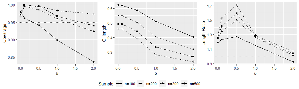
Figure 4: Dependence on $\delta$ and $n$ (setting 1). “Coverage” and “CI Length” stand for the empirical coverage and the average length of our proposed CI, respectively; “Length Ratio” represents the ratio of the average length of our proposed CI to the normality CI in (33).

(a) Setting 3(a) with covariate shift

(b) Setting 3(b) with no covariate shift

Figure 5: Comparison of covariate shift and no covariate shift algorithms ($n=500$). “CS Known”, “CS” and “No CS” represent Algorithm 1 with known $\Sigma^{\mathbb{Q}}$, Algorithm 1, and Algorithm 1 with no covariate shift, respectively. “Coverage” and “CI Length” stand for the empirical coverage and the average length of our proposed CI, respectively; “Length Ratio” represents the ratio of the average length of our proposed CI to the normality CI.

Covariate shift. We modify Algorithm 1 to two extra scenarios: (1) $\Sigma^{\mathbb{Q}}$ is known; (2) no covariate shift between the target and source populations. In both scenarios, we present how to construct a debiased estimator $\widehat{\Gamma}^{\mathbb{Q}}$ in Section A.3 in the supplement. We then implement Algorithm 1 with the modified $\widehat{\Gamma}^{\mathbb{Q}}$. We shall refer to the corresponding methods as Algorithm 1 with known $\Sigma^{\mathbb{Q}}$ and Algorithm 1 with no covariate shift.

The top of Figure 5 corresponds to the simulation settings with covariate shift and $n=500$. The no covariate shift algorithm does not achieve 95% coverage due to the bias of assuming no covariate shift. In contrast, the covariate shift algorithms (with or without knowing $\Sigma^{\mathbb{Q}}$) achieve the 95% coverage level, and the CI constructed with known $\Sigma^{\mathbb{Q}}$ is shorter as it does not need to quantify the uncertainty of estimating $\Sigma^{\mathbb{Q}}.$ The bottom of Figure 5 corresponds to the setting with no covariate shift. All algorithms achieve the desired coverage level. The results for $n=200$ are reported in Figure S2 in the supplement.

8 Real Data Applications

We analyze a genome-wide association study (Bloom et al., 2013) on yeast colony growth based on $n=1008$ saccharomyces cerevisiae segregants crossbred from a laboratory and a wine strain. Bloom et al. (2013) selected $4410$ Single Nucleotide Polymorphisms (SNPs) for the data analysis. We further apply LD screening (Calus and Vandenplas, 2018) to remove SNPs with absolute correlation above $0.85$ and end up with $p=513$ SNPs for the regression analysis. The outcome variables are the end-point colony sizes under different growth media. These outcome variables are normalized to have a variance of $1$. We consider four source growth media: “Ethanol”, “Lactose”, “5-Fluorouracil”, and “Xylose”. The model (1) is applied here with $L=4$, and each $1\leq l\leq 4$ corresponds to the data for one growth medium.

We start with the preliminary analysis of whether the regression vectors in (1) are heterogeneous across the four growth media. For $1\leq l\leq 4$, we construct the debiased lasso estimator $\widehat{b}^{(l)}_{j}$ as in (13) with $w=e_{j}$ for $1\leq j\leq p,$ and obtain the corresponding covariance matrix as ${\rm Cov}(\widehat{b}^{(l)})\in\mathbb{R}^{p\times p}.$ For $1\leq l_{1}<l_{2}\leq L$, we test $H_{0}:{b}^{(l_{1})}={b}^{(l_{2})}$ by extending the bootstrap methods in Dezeure et al. (2017). We generate the bootstrap samples $Z^{(1)},\cdots,Z^{(1000)}$ following $Z^{(k)}\sim N\left({\bf 0},{\rm Cov}(\widehat{b}^{(l_{1})})+{\rm Cov}(\widehat{b}^{(l_{2})})\right)$ for $1\leq k\leq 1000.$ We compute the maximum statistics $T^{(l_{1},l_{2})}_{\rm obs}=\max_{1\leq j\leq p}|\widehat{b}^{(l_{1})}_{j}-\widehat{b}^{(l_{2})}_{j}|$ and calculate the p-value as $\frac{1}{1000}\sum_{k=1}^{1000}{\bf 1}(\|Z^{(k)}\|_{\infty}\geq T^{(l_{1},l_{2})}_{\rm obs})$. As reported in Table 3, the small p-values indicate the data heterogeneity across the four media.

	Ethanol	Lactose	5-Fluorouracil	Xylose
Ethanol	-	0.001	0.059	0.146
Lactose	-	-	0.001	0.003
5-Fluorouracil	-	-	-	0.027

Table 3: p-values for homogeneity test of regression vectors in (1). For example, $0.003$ stands for the p-value of testing whether the regression vectors for media “Lactose” and “Xylose” are the same.

8.1 Maximin effects: summary of stable associations across source media

In Figure 6, we demonstrate that the maximin effect summarizes the stable associations across the four source media. In particular, an SNP with a significant maximin effect tends to have consistent effects across source media. Due to space constraints, we report the inference results for a representative subset $\mathcal{S}$ of SNPs in Figure 6 rather than reporting results for all $513$ SNPs used for the regression analysis. Figure 6 illustrates that SNPs with indexes $420,443,437,423,245,424$ have homogeneous effects across the source media, and the corresponding maximin effect is significant. The gene KRE33 containing SNP $420$ is an essential gene for yeast (Cherry et al., 2012), which is a gene absolutely required to maintain life provided that all nutrients are available (Zhang and Lin, 2009).

Figure 6: The top panel plots debiased estimators and corresponding CIs for $\{b^{(l)}_{j}\}_{1\leq l\leq 4,j\in\mathcal{S}}$ with the index set $\mathcal{S}=\{420,443,437,423,245,424,364,229,6,177,63,84\}$. The bottom panel plots CIs for $\{[\beta^{*}_{\delta}]_{j}\}_{j\in\mathcal{S}}$ in the no covariate shift setting with $\delta\in\{0,0.2,0.5\}$.

Figure 6 also illustrates the SNPs with insignificant maximin effects, which correspond to the following three types of heterogeneous regression effects: (1) the SNPs (e.g., with indexes 364, 229) have opposite effects across different media; (2) the SNPs (e.g., with indexes 6, 177) only have a significant effect on one medium; (3) the SNPs (e.g., with indexes 63, 84) do not have any significant effect across different growth media. Figure 6 shows that the CIs for the ridge-type maximin effect get shorter with a larger penalty level $\delta$, which is coherent with the simulation results reported in Figures 4 and 5.

8.2 Generalizability of maximin effects to test media

We demonstrate the generalizability of the maximin effect by examining seven test media: “Lactate”, “SDS”, “Trehalose”, “6-Azauracil”, “YNB”, “YPD”, and “YPD.4C”. In this application, the target distribution $\mathbb{Q}$ represents the joint distribution of $p=513$ SNPs and the colony growth size under a specific test medium. There is no covariate shift since the covariates observations are the same across different growth media, and the only difference is the outcome variable (colony size). Due to the difference in growth media, the conditional outcome distribution $\mathbb{Q}_{Y|X}$ in the test media will likely differ from $\{\mathbb{P}^{(l)}_{Y|X}\}_{1\leq l\leq 4}$ in the source media. The outcome observations for the seven test media are only used to validate the maximin effect’s generalizability instead of constructing the maximin effect.

In the following, we examine whether the stable associations captured by the maximin effect can be generalized to the test media. Mainly, we investigate whether the SNPs with significant maximin effects also have significant effects in the test media. We use each test medium’s own SNP and outcome data and conduct multiple testing to choose SNPs with significant effects. We report the results in Table 4, where we adjust for the multiplicity by applying the BH procedure (Benjamini and Hochberg, 1995) and controlling FDR below $0.1$.

	Media name	Number	Indexes of significant SNPs
Source Media	Ethanol	6	73,186,419,420,423,443
	Lactose	5	323,420,442,443,451
	5-Fluorouracil	16	16,126,130,282,330,364,366,396,399,420,423,424,442,458,462,497
	Xylose	12	73,80,207,245,356,364,420,423,437,443,459,496
Test Media	Lactate	6	1,53,324,420,437,443
	SDS	5	256,257,364,420,459
	Trehalose	9	1,79,324,349,364,420,437,443,496
	6-Azauracil	6	73,420,424,437,442,459
	YNB	9	27,207,208,254,282,420,423,442,499
	YPD	12	24,73,207,231,359,420,423,424,437,442,443,459
	YPD.4C	6	73,342,364,420,423,459

Table 4: Significant SNPs for each growth medium after controlling the FDR below $0.1$; for example, for the “Ethanol” medium, there are 6 significant SNPs with indexes $73,186,419,420,423,443.$

We conduct the maximin significance test by applying the BH procedure to the p-values defined in (22) and controlling the false discovery rate (FDR) below $0.1$. After adjusting for multiplicity, we obtain the maximin significant SNPs as $\{420,423,437,443\}.$ In Figure 7, we plot a subset of SNPs that are maximin significant or significant in at least one source or test media. For every SNP, we report the number of growth media on which it has significant effects. Of all eleven media, SNP 420 is significant in all, SNPs 423 and 443 are significant in six, and SNP 437 is significant in five. The maximin significant SNPs $\{420,423,437,443\}$ are shown to have generalizable effects for the test media. As reported in Table 4, the SNP 420 is significant in all seven test media, the SNP 437 is significant in four test media, and the SNPs 423 and 443 are significant in three test media. Figure 7 also demonstrates that a larger group of maximin significant SNPs can be identified after increasing the ridge penalty $\delta$, where the identified SNPs 442 and 424 are significant in three and two test media, respectively. We report the names of the genes containing the maximin significant SNPs in Table S4 in the supplement.

Figure 7: The y-axis represents the number of media, and the x-axis represents the SNP indexes. As an example, the SNP 420 is significant over 11 media. The red color indicates the maximin significance. The top, middle, and bottom panels correspond to the maximin effects with no ridge penalty, penalty $\delta=0.2$, and $\delta=0.5$, respectively.

Figure 7 demonstrates that the maximin significant SNPs are likely replicable for source and test media. We compare our maximin integration to the empirical risk minimization (ERM), which pools over the data from four source media and implements the standard debiased estimators and the following-up FDR control on this combined data. The ERM method identifies significant SNPs $\{420,423,437,246,357,419\}$ with the SNPs $\{420,423,437\}$ being also identified as maximin significant. The important SNP 443 is maximin significant but not identified using ERM. Moreover, the ERM method selects some SNPs without generalizable effects: the SNP 419 is only identified as significant over a single source medium but not any test medium; the SNPs $246,357$ are insignificant over any of the eleven growth media. This comparison illustrates that the maximin integration identifies SNPs with more generalizable effects across different environments than the ERM method. The stable associations summarized by maximin effects are easier to generalize to the target populations, which might have potential distribution shifts resulting from the different growth media used.

9 Conclusion and Discussions

This paper advocates integrating multi-source data with maximin effects, a new data-fusion tool extracting generalizable information from heterogeneous data. The stable associations summarized by the maximin effects are more likely to generalize to a range of target populations that may have distributional shifts from the source populations. The maximin integration contrasts with other multi-source learning algorithms, including the meta-analysis and the regression analysis based on the merged data, which do not accommodate the distributional shifts between the source and target populations. Our proposed sampling approach addresses inference challenges arising in the maximin integration and helps address other non-standard inference problems. Interesting directions include inference for maximin effects when the linear models in (1) are misspecified (Wasserman, 2014; Bühlmann and van de Geer, 2015) and construction of distributionally robust models with machine learning prediction models. Both questions are left for future research.

Supplement

The supplement contains all proofs and additional methods, theories, and numerical results.

Supplement to “Inference for Maximin Effects:
Identifying Stable Associations across Multiple Studies”

The supplementary materials are organized as follows,

1. In Section A, we provide additional discussions, methods, and theories.

2. In Section B, we further discuss the non-regularity and instability challenges for confidence interval construction with bootstrap and subsampling methods.

3. We present the proofs of Theorems 1 and 2 in Sections D and E, respectively. In Section C, we present the proofs of Propositions 1 to 6. In Section F, we provide the proofs of extra lemmas.

4. In Section G, we present additional numerical studies.

Additional notations

. For positive sequences $a_{n}$ and $b_{n}$, $a_{n}\lesssim b_{n}$ means that $\exists C>0$ such that $a_{n}\leq Cb_{n}$ for all $n$; $a_{n}\asymp b_{n}$ if $a_{n}\lesssim b_{n}$ and $b_{n}\lesssim a_{n}$, and $a_{n}\ll b_{n}$ if $\limsup_{n\rightarrow\infty}{a_{n}}/{b_{n}}=0$. For a set $S$, $\left|S\right|$ denotes its cardinality and $S^{c}$ denotes its complement. For a vector $x\in\mathbb{R}^{p}$ and a subset $S\subset[p]$, $x_{S}$ is the sub-vector of $x$ with indices in $S$ and $x_{-S}$ is the sub-vector with indices in $S^{c}$. The $\ell_{q}$ norm of a vector $x$ is defined as $\|x\|_{q}=\left(\sum_{l=1}^{p}|x_{l}|^{q}\right)^{\frac{1}{q}}$ for $q\geq 0$ with $\|x\|_{0}=\left|\{1\leq l\leq p:x_{l}\neq 0\}\right|$ and $\|x\|_{\infty}=\max_{1\leq l\leq p}|x_{l}|$. For a matrix $A$, we use $\lambda_{j}(A)$, $\|A\|_{F}$, $\|A\|_{2}$ and $\|A\|_{\infty}$ to denote its $j$-th largest singular value, Frobenius norm, spectral norm, and element-wise maximum norm, respectively. For a matrix $X$, $X_{i}$ and $X_{\cdot,j}$ are used to denote its $i$-th row and $j$-th column, respectively; for index sets $S_{1}$ and $S_{2}$, $X_{S_{1},S_{2}}$ denotes the sub-matrix of $X$ with row and column indices belonging to $S_{1}$ and $S_{2},$ respectively; $X_{S_{1}}$ denotes the sub-matrix of $X$ with row indices belonging to $S_{1}.$ For random objects $X_{1}$ and $X_{2}$, we use $X_{1}\stackrel{{\scriptstyle d}}{{=}}X_{2}$ to denote that they are equal in distribution. For a sequence of random variables $X_{n}$ indexed by $n$, we use $X_{n}\overset{p}{\to}X$ and $X_{n}\overset{d}{\to}X$ to represent that $X_{n}$ converges to $X$ in probability and in distribution, respectively.

Appendix A Additional Discussions

In Section A.1, we discuss the connection to minimax group fairness. In Section A.2, we formulate the maximin projection as a form of the covariate-shift maximin effect. In Section A.3, we provide the details on inference for $\Gamma^{\mathbb{Q}}$ in high dimensions.

A.1 Minimax Group Fairness and Rawlsian Max-min Principle

Fairness is an important consideration for designing the machine learning algorithm. In particular, the algorithm trained to maximize average performance on the training data set might under-serve or even cause harm to a sub-population of individuals (Dwork et al., 2012). The goal of the group fairness is to build a model satisfying a certain fairness notation (e.g. statistical parity) across predefined sub-populations. However, such fairness notation can be typically achieved by downgrading the performance on the benefitted groups without improving the disadvantaged ones (Martinez et al., 2020; Diana et al., 2021). To address this, Martinez et al. (2020); Diana et al. (2021) proposed the minimax group fairness algorithm which ensures certain fairness principle and also maximizes the utility for each sub-population. We assume that we have access to the i.i.d data $\{Y_{i},X_{i},A_{i}\}_{1\leq i\leq n}$, where for the $i$-th observation, $Y_{i}$ and $X_{i}\in\mathbb{R}^{p}$ denote the outcome and the covariates, respectively, and $A_{i}$ denotes the sensitive variable (e.g. age or sex). The training data can be separated into different sub-groups depending on the value of the sensitive variable $A_{i}.$ For a discrete $A_{i}$, we use $\mathcal{A}$ to denote the set of all possible values that $A_{i}$ can take. Then the minimax group fairness can be defined as

$$\beta^{\rm mm-fair}:=\operatorname*{arg\,min}_{\beta}\max_{a\in\mathcal{A}}\mathbf{E}_{Y_{i},X_{i}\mid A_{i}=a}\ell(Y_{i},X_{i}^{\intercal}\beta)=\operatorname*{arg\,max}_{\beta}\min_{a\in\mathcal{A}}\mathbf{E}_{Y_{i},X_{i}\mid A_{i}=a}[-\ell(Y_{i},X_{i}^{\intercal}\beta)]$$

where $\ell(Y_{i},X_{i}^{\intercal}\beta)$ denotes a loss function and $-\ell(Y_{i},X_{i}^{\intercal}\beta)$ can be viewed as a reward/utility function. In terms of utility maximization, the idea of minimax group fairness estimator dates at least back to Rawlsian max-min fairness (Rawls, 2001). When the distribution of $X_{i}$ does not change with the value of $A_{i}$, then minimax group fairness estimator $\beta^{\rm mm-fair}$ is equivalent to the minimax or the maximin estimator, where the group label is determined by the value of $A_{i}.$

A.2 Individualized Treatment Effect: Maximin Projection

Shi et al. (2018) proposed the maximin projection algorithm to construct the optimal treatment regime for new patients by leveraging training data from different groups with heterogeneity in optimal treatment decision. As explained in Shi et al. (2018), the heterogeneity in optimal treatment decision might come from patients’ different enrollment periods and/or the treatment quality from different healthcare centers. Particularly, Shi et al. (2018) considered that the data is collected from $L$ heterogeneous groups. For the $l$-th group with $1\leq l\leq L$, let $Y^{(l)}_{i}\in\mathbb{R}$, $A^{(l)}_{i}$ and $X^{(l)}_{i}\in\mathbb{R}^{p}$ denote the outcome, the treatment and the baseline covariates, respectively. Shi et al. (2018) considered the following model for the data in group $l$,

$$Y^{(l)}_{i}=h_{l}(X^{(l)}_{i})+A^{(l)}_{i}\cdot[(b^{(l)})^{\intercal}X^{(l)}_{i}+c]+e^{(l)}_{i}\quad\text{with}\quad\mathbf{E}(e^{(l)}_{i}\mid X^{(l)}_{i},A^{(l)}_{i})=0,$$

where $h_{l}:\mathbb{R}^{p}\rightarrow\mathbb{R}$ denotes the unknown baseline function for the group $l$ and the vector $b^{(l)}\in\mathbb{R}^{p}$ describes the individualized treatment effect. To address the heterogeneity in optimal treatment regimes, Shi et al. (2018) has proposed the maximum projection

$$\beta^{*,{\rm MP}}=\operatorname*{arg\,max}_{\|\beta\|_{2}\leq 1}\min_{1\leq l\leq L}\beta^{\intercal}b^{(l)}.$$ (34)

After identifying $\beta^{*,{\rm MP}},$ we may construct the treatment regime for a new patient with covariates $w$ by testing

$$H_{0}:w^{\intercal}\beta^{*,{\rm MP}}+c<0.$$ (35)

The following Proposition 3 identifies the maximin projection $\beta^{*,{\rm MP}}.$ Through comparing it with Proposition 1, we note that the maximin projection is proportional to the general maximin effect defined in (7) with $\Sigma^{\mathbb{Q}}={\rm I}$ and hence the identification of $\beta^{*}(\mathbb{I})$ is instrumental in identifying $\beta^{*,{\rm MP}}$, which provides the strong motivation for statistical inference for $w^{\intercal}\beta^{*}(\mathbb{I}).$

Proposition 3.

The maximum projection $\beta^{*,{\rm MP}}$ in (34) satisfies $\beta^{*,{\rm MP}}=\frac{1}{\|\beta^{*}({\mathbb{I}})\|_{2}}\beta^{*}({\mathbb{I}})$ with $\beta^{*}({\mathbb{I}})=\sum_{l=1}^{L}\gamma^{*}_{l}b^{(l)}$ where $\gamma^{*}=\operatorname*{arg\,min}_{\gamma\in\Delta^{L}}\gamma^{\intercal}\Gamma^{\mathbb{I}}\gamma$ and $\Gamma_{lk}^{\mathbb{I}}=(b^{(l)})^{\intercal}b^{(k)}$ for $1\leq l,k\leq L.$

We refer to Shi et al. (2018) for more details on the maximin projection in the low-dimensional setting. Our proposed sampling method in Section 4 is useful in devising statistical inference methods for $\beta^{*,{\rm MP}}$ in high dimensions.

A.3 Debiased Estimators of $\Gamma^{\mathbb{Q}}$

We present the details about constructing the debiased estimator ${\widehat{\Gamma}_{l,k}}^{\mathbb{Q}}$ in (15). We estimate $\{b^{(l)}\}_{1\leq l\leq L}$ by applying Lasso (Tibshirani, 1996) to the sub-sample with the index set $A_{l}$:

$$\widehat{b}_{init}^{(l)}=\operatorname*{arg\,min}_{b\in\mathbb{R}^{p}}\frac{\|Y^{(l)}_{A_{l}}-X^{(l)}_{A_{l}}b\|_{2}^{2}}{2|A_{l}|}+{\lambda_{l}}\sum_{j=1}^{p}\frac{\|X^{(l)}_{A_{l},j}\|_{2}}{\sqrt{|A_{l}|}}|b_{j}|,\;\text{with}\;\lambda_{l}=\sqrt{\frac{(2+c)\log p}{|A_{l}|}}\sigma_{l}$$ (36)

for some constant $c>0.$ The Lasso estimators $\{\widehat{b}^{(l)}_{init}\}_{1\leq l\leq L}$ are implemented by the R-package glmnet (Friedman et al., 2010) with tuning parameters $\{\lambda_{l}\}_{1\leq l\leq L}$ chosen by cross validation. We may also construct the initial estimator $\widehat{b}_{init}^{(l)}$ by tuning-free penalized estimators (Sun and Zhang, 2012; Belloni et al., 2011). Define

$$\widehat{\Sigma}^{\mathbb{Q}}=\frac{1}{|B|}\sum_{i\in B}X^{\mathbb{Q}}_{i}(X^{\mathbb{Q}}_{i})^{\intercal},\quad\widehat{\Sigma}^{(l)}=\frac{1}{|B_{l}|}\sum_{i\in B_{l}}X^{(l)}_{i}[X^{(l)}_{i}]^{\intercal},\quad\widetilde{\Sigma}^{\mathbb{Q}}=\frac{1}{|A|}\sum_{i\in A}X^{\mathbb{Q}}_{i}(X^{\mathbb{Q}}_{i})^{\intercal}.$$

For $1\leq l,k\leq L$, the plug-in estimator $[\widehat{b}_{init}^{(l)}]^{\intercal}\widehat{\Sigma}^{\mathbb{Q}}\widehat{b}_{init}^{(k)}$ has the error decomposition:

$$(\widehat{b}_{init}^{(l)})^{\intercal}\widehat{\Sigma}^{\mathbb{Q}}\widehat{b}_{init}^{(k)}-(b^{(l)})^{\intercal}\Sigma^{\mathbb{Q}}b^{(k)} =(\widehat{b}_{init}^{(k)})^{\intercal}\widehat{\Sigma}^{\mathbb{Q}}(\widehat{b}_{init}^{(l)}-b^{(l)})+(\widehat{b}_{init}^{(l)})^{\intercal}\widehat{\Sigma}^{\mathbb{Q}}(\widehat{b}_{init}^{(k)}-b^{(k)})$$

$$-(\widehat{b}_{init}^{(l)}-b^{(l)})^{\intercal}\widehat{\Sigma}^{\mathbb{Q}}(\widehat{b}_{init}^{(k)}-b^{(k)})+(b^{(l)})^{\intercal}(\widehat{\Sigma}^{\mathbb{Q}}-\Sigma^{\mathbb{Q}})b^{(k)}.$$

The debiased estimator in (15) is to correct the plug-in estimator $[\widehat{b}_{init}^{(l)}]^{\intercal}\widehat{\Sigma}^{\mathbb{Q}}\widehat{b}_{init}^{(k)}$ by approximating the estimation error $(\widehat{b}_{init}^{(k)})^{\intercal}\widehat{\Sigma}^{\mathbb{Q}}(\widehat{b}_{init}^{(l)}-b^{(l)})$ with $-\frac{1}{|B_{l}|}[\widehat{u}^{(l,k)}]^{\intercal}[X^{(l)}_{B_{l}}]^{\intercal}(Y^{(l)}_{B_{l}}-X^{(l)}_{B_{l}}\widehat{b}_{init}^{(l)}),$ where the projection direction $\widehat{u}^{(l,k)}$ is constructed as follows,

$$\widehat{u}^{(l,k)}=\;\operatorname*{arg\,min}_{u\in\mathbb{R}^{p}}u^{\intercal}\widehat{\Sigma}^{(l)}u\quad\text{subject to} \;\|\widehat{\Sigma}^{(l)}u-\omega^{(k)}\|_{\infty}\leq\|\omega^{(k)}\|_{2}\mu_{l}$$ (37)

$$\;\left|[\omega^{(k)}]^{\intercal}\widehat{\Sigma}^{(l)}u-\|\omega^{(k)}\|_{2}^{2}\right|\leq\|\omega^{(k)}\|_{2}^{2}\mu_{l}$$ (38)

$$\;\left\|X_{B_{l}}u\right\|_{\infty}\leq\|\omega^{(k)}\|_{2}\tau_{l}$$ (39)

with $\mu_{l}\asymp\sqrt{\log p/|B_{l}|}$, $\tau_{l}\asymp\sqrt{\log n_{l}},$ and

$$\omega^{(k)}=\widetilde{\Sigma}^{\mathbb{Q}}\widehat{b}_{init}^{(k)}\in\mathbb{R}^{p}.$$ (40)

Similarly, we approximate the bias $(\widehat{b}_{init}^{(l)})^{\intercal}\widehat{\Sigma}^{\mathbb{Q}}(\widehat{b}_{init}^{(k)}-b^{(k)})$ by $-\frac{1}{|B_{k}|}[\widehat{u}^{(k,l)}]^{\intercal}[X^{(k)}_{B_{k}}]^{\intercal}(Y^{(k)}_{B_{k}}-X^{(k)}_{B_{k}}\widehat{b}_{init}^{(k)}).$

We decompose the error of approximating $(\widehat{b}_{init}^{(k)})^{\intercal}\widehat{\Sigma}^{\mathbb{Q}}(\widehat{b}_{init}^{(l)}-b^{(l)})$ by $-\frac{1}{|B_{l}|}[\widehat{u}^{(l,k)}]^{\intercal}[X^{(l)}_{B_{l}}]^{\intercal}(Y^{(l)}_{B_{l}}-X^{(l)}_{B_{l}}\widehat{b}_{init}^{(l)})$ as

$$-\frac{1}{|B_{l}|}[\widehat{u}^{(l,k)}]^{\intercal}[X^{(l)}_{B_{l}}]^{\intercal}\epsilon^{(l)}_{B_{l}}+[\widehat{\Sigma}^{(l)}\widehat{u}^{(l,k)}-\widehat{\Sigma}^{\mathbb{Q}}\widehat{b}_{init}^{(k)}]^{\intercal}(\widehat{b}_{init}^{(l)}-b^{(l)}).$$ (41)

We now provide intuitions on why the projection direction $\widehat{u}^{(l,k)}$ proposed in (37), (38) and (39) ensures a small approximation error in (41). The objective $u^{\intercal}\widehat{\Sigma}^{(l)}u$ in (37) is proportional to the variance of the first term in (41). The constraint set in (37) implies $\widehat{\Sigma}^{(l)}\widehat{u}^{(l,k)}-\widehat{\Sigma}^{\mathbb{Q}}\widehat{b}_{init}^{(k)}\approx\widehat{\Sigma}^{(l)}\widehat{u}^{(l,k)}-\omega^{(k)}\approx{\bf 0},$ which guarantees the second term of (41) to be small. The additional constraint (38) is seemingly useless to control the approximation error in (41). However, this additional constraint ensures that the first term in (41) dominates the second term in (41), which is critical in constructing an asymptotically normal estimator of $\Gamma^{\mathbb{Q}}_{l,k}.$ The additional constraint (38) is particularly useful in the covariate shift setting, that is, $\Sigma^{(l)}\neq\Sigma^{\mathbb{Q}}$ for some $1\leq l\leq L.$ The last constraint (39) is useful in establishing the asymptotic normality of the debiased estimator for non-Gaussian errors. We believe that the constraint (39) is only needed for technical reasons.

To construct $\widehat{u}^{(l,k)}$ in (15), we solve the dual problem of (37) and (38),

$$\widehat{h}=\operatorname*{arg\,min}_{h\in\mathbb{R}^{p+1}}h^{\intercal}H^{\intercal}\widehat{\Sigma}^{(l)}Hh/4+(\omega^{(k)})^{\intercal}Hh/{\|\omega^{(k)}\|_{2}}+\lambda\|h\|_{1}\;\text{with}\;H=\left[\begin{matrix}{\omega^{(k)}}/{\|\omega^{(k)}\|_{2}},\mathbf{I}_{p\times p}\end{matrix}\right],$$ (42)

where we adopt the notation $0/0=0$. The objective value of this dual problem is unbounded from below when $H^{\intercal}\widehat{\Sigma}^{(l)}H$ is singular and $\lambda$ is near zero. We choose the smallest $\lambda>0$ such that the dual problem is bounded from below and construct $\widehat{u}^{(l,k)}=-\tfrac{1}{2}(\widehat{h}_{-1}+\widehat{h}_{1}{\omega^{(k)}}/{\|\omega^{(k)}\|_{2}}).$

We estimate the covariance between $\widehat{\Gamma}^{\mathbb{Q}}_{l_{1},k_{1}}-{\Gamma}^{\mathbb{Q}}_{l_{1},k_{1}}$ and $\widehat{\Gamma}^{\mathbb{Q}}_{l_{2},k_{2}}-{\Gamma}^{\mathbb{Q}}_{l_{2},k_{2}}$ by

$$\widehat{\bf V}_{\pi(l_{1},k_{1}),\pi(l_{2},k_{2})}=\widehat{\bf V}^{(a)}_{\pi(l_{1},k_{1}),\pi(l_{2},k_{2})}+\widehat{\bf V}^{(b)}_{\pi(l_{1},k_{1}),\pi(l_{2},k_{2})},$$

where

$$\widehat{\bf V}^{(a)}_{\pi(l_{1},k_{1}),\pi(l_{2},k_{2})}= \frac{\widehat{\sigma}_{l_{1}}^{2}}{|B_{l_{1}}|}(\widehat{u}^{(l_{1},k_{1})})^{\intercal}\widehat{\Sigma}^{(l_{1})}\left[\widehat{u}^{(l_{2},k_{2})}{\bf 1}(l_{2}=l_{1})+\widehat{u}^{(k_{2},l_{2})}{\bf 1}(k_{2}=l_{1})\right]+$$ (43)

$$\frac{\widehat{\sigma}_{k_{1}}^{2}}{|B_{k_{1}}|}(\widehat{u}^{(k_{1},l_{1})})^{\intercal}\widehat{\Sigma}^{(k_{1})}\left[\widehat{u}^{(l_{2},k_{2})}{\bf 1}(l_{2}=k_{1})+\widehat{u}^{(k_{2},l_{2})}{\bf 1}(k_{2}=k_{1})\right],$$

and

$$\widehat{\bf V}^{(b)}_{\pi(l_{1},k_{1}),\pi(l_{2},k_{2})}={\frac{1}{|B|N_{\mathbb{Q}}}\sum_{i=1}^{N_{\mathbb{Q}}}\left((\widehat{b}_{init}^{(l_{1})})^{\intercal}X_{i}^{\mathbb{Q}}(\widehat{b}_{init}^{(k_{1})})^{\intercal}X_{i}^{\mathbb{Q}}(\widehat{b}_{init}^{(l_{2})})^{\intercal}X_{i}^{\mathbb{Q}}(\widehat{b}_{init}^{(k_{2})})^{\intercal}X_{i}^{\mathbb{Q}}-(\widehat{b}_{init}^{(l_{1})})^{\intercal}\bar{\Sigma}^{\mathbb{Q}}\widehat{b}_{init}^{(k_{1})}(\widehat{b}_{init}^{(l_{2})})^{\intercal}\bar{\Sigma}^{\mathbb{Q}}\widehat{b}_{init}^{(k_{2})}\right)}$$ (44)

with $\widehat{\sigma}_{l}^{2}$ defined in (14), $\bar{\Sigma}^{\mathbb{Q}}=\frac{1}{N_{\mathbb{Q}}}\sum_{i=1}^{N_{\mathbb{Q}}}X_{i}^{\mathbb{Q}}(X_{i}^{\mathbb{Q}})^{\intercal}$, and $\widehat{\Sigma}^{(l)}=\frac{1}{|B_{l}|}\sum_{i\in B_{l}}X^{(l)}_{i}[X^{(l)}_{i}]^{\intercal}$ for $1\leq l\leq L,$

Remark 6.

If $\Sigma^{\mathbb{Q}}$ is known, we modify ${\widehat{\Gamma}_{l,k}}^{\mathbb{Q}}$ in (15) by replacing $\widehat{\Sigma}^{\mathbb{Q}}$ by $\Sigma^{\mathbb{Q}}$ and $\omega^{(k)}$ in (40) by $\omega^{(k)}=\Sigma^{\mathbb{Q}}\widehat{b}_{init}^{(k)}.$ The covariance matrix of the estimator (with known $\Sigma^{\mathbb{Q}}$) will be $\widehat{{\bf V}}^{(a)}$ defined in (46) since $\widehat{{\bf V}}^{(b)}$ is used to quantify the uncertainty of estimating $\Sigma^{\mathbb{Q}}$ but there is no uncertainty of estimating $\Sigma^{\mathbb{Q}}.$ The estimator constructed with the knowledge of $\Sigma^{\mathbb{Q}}$ typically has a smaller variance than the estimator ${\widehat{\Gamma}_{l,k}}^{\mathbb{Q}}$ in (15) since there is no uncertainty of estimating $\Sigma^{\mathbb{Q}}$; see Figure 5 in the main paper for numerical comparisons.

A.3.1 Theoretical Justification

In the following, we provide the theoretical guarantee of our proposed estimator $\widehat{\Gamma}^{\mathbb{Q}}_{l,k}.$ Define

$${\bf V}_{\pi(l_{1},k_{1}),\pi(l_{2},k_{2})}={\bf V}^{(a)}_{\pi(l_{1},k_{1}),\pi(l_{2},k_{2})}+{\bf V}^{(b)}_{\pi(l_{1},k_{1}),\pi(l_{2},k_{2})},$$ (45)

with

$${\bf V}^{(a)}_{\pi(l_{1},k_{1}),\pi(l_{2},k_{2})} =\frac{\sigma_{l_{1}}^{2}}{|B_{l_{1}}|}(\widehat{u}^{(l_{1},k_{1})})^{\intercal}\widehat{\Sigma}^{(l_{1})}\left[\widehat{u}^{(l_{2},k_{2})}{\bf 1}(l_{2}=l_{1})+\widehat{u}^{(k_{2},l_{2})}{\bf 1}(k_{2}=l_{1})\right]$$ (46)

$$+\frac{\sigma_{k_{1}}^{2}}{|B_{k_{1}}|}(\widehat{u}^{(k_{1},l_{1})})^{\intercal}\widehat{\Sigma}^{(k_{1})}\left[\widehat{u}^{(l_{2},k_{2})}{\bf 1}(l_{2}=k_{1})+\widehat{u}^{(k_{2},l_{2})}{\bf 1}(k_{2}=k_{1})\right],$$

and

$${\bf V}^{(b)}_{\pi(l_{1},k_{1}),\pi(l_{2},k_{2})}=\frac{1}{|B|}(\mathbf{E}[b^{(l_{1})}]^{\intercal}X_{i}^{\mathbb{Q}}[b^{(k_{1})}]^{\intercal}X_{i}^{\mathbb{Q}}[b^{(l_{2})}]^{\intercal}X_{i}^{\mathbb{Q}}[b^{(k_{2})}]^{\intercal}X_{i}^{\mathbb{Q}}-(b^{(l_{1})})^{\intercal}\Sigma^{\mathbb{Q}}b^{(k_{1})}(b^{(l_{2})})^{\intercal}\Sigma^{\mathbb{Q}}b^{(k_{2})}).$$ (47)

Our analysis relies on the asymptotic normality of the point estimator $\widehat{\Gamma}^{\mathbb{Q}}$. However, we shall emphasize that our analysis only requires the following Proposition 4, which establishes that the marginal distribution of $\widehat{\Gamma}_{l,k}^{\mathbb{Q}}-\Gamma_{l,k}^{\mathbb{Q}}$ is approximately normal. This marginal limiting distribution is a weaker requirement than the joint asymptotic normality of $\{\widehat{\Gamma}_{l,k}^{\mathbb{Q}}-\Gamma_{l,k}^{\mathbb{Q}}\}_{1\leq k\leq l\leq L}$. However, the results established in the following proposition is already sufficient for our use of proving Theorem 1. We present its proof at Section C.7.

Proposition 4.

Consider the model (1). Suppose that Conditions (A1) and (A2) hold, then the estimator $\widehat{\Gamma}^{\mathbb{Q}}$ in (15) satisfies (48)

$$\liminf_{n,p\rightarrow\infty}{\mathbf{P}}\left(\max_{1\leq l,k\leq L}\frac{\left|\widehat{\Gamma}_{l,k}^{\mathbb{Q}}-\Gamma_{l,k}^{\mathbb{Q}}\right|}{\sqrt{\widehat{{\bf V}}_{\pi(l,k),\pi(l,k)}+d_{0}/n}}\leq 1.05\cdot z_{{\alpha_{0}}/[L(L+1)]}\right)\geq 1-\alpha_{0},$$ (48)

for any $\alpha_{0}\in(0,0.01].$

The proof of Proposition 4 relies on the following Propositions 5 and 6. The proofs of Propositions 5 and 6 can be found in Sections C.6 and C.5, respectively.

Proposition 5.

Consider the model (1). Suppose Condition (A1) holds, $\tfrac{s\log p}{\min\{n,N_{\mathbb{Q}}\}}\rightarrow 0$ with $n=\min_{1\leq l\leq L}n_{l}$ and $s=\max_{1\leq l\leq L}\|b^{(l)}\|_{0}$. Then the proposed estimator $\widehat{\Gamma}^{\mathbb{Q}}_{l,k}\in\mathbb{R}^{L\times L}$ in (15) in the main paper satisfies $\widehat{\Gamma}^{\mathbb{Q}}_{l,k}-\Gamma^{\mathbb{Q}}_{l,k}=D_{l,k}+{\rm Rem}_{l,k},$ where

$$\frac{D_{l,k}}{\sqrt{{\bf V}_{\pi(l,k),\pi(l,k)}}}\overset{d}{\to}\mathcal{N}(0,1),$$ (49)

with ${\bf V}$ defined in (45); for $1\leq l,k\leq L,$ with probability larger than $1-\min\{n,p\}^{-c}$ for a constant $c>0,$ the reminder term ${\rm Rem}_{l,k}$ satisfies

$$\left|{\rm Rem}_{l,k}\right|\lesssim(1+\|\omega^{(k)}\|_{2}+\|\omega^{(l)}\|_{2})\frac{s\log p}{n}+(\|b^{(k)}\|_{2}+\|b^{(l)}\|_{2})\sqrt{\frac{s(\log p)^{2}}{nN_{\mathbb{Q}}}},$$ (50)

where $c>0$ is a positive constant and $\omega^{(k)}$ and $\omega^{(l)}$ are defined in (40).

Proposition 6.

Suppose that the assumptions of Proposition 5 hold. Then with probability larger than $1-\min\{n,p\}^{-c}$, the diagonal element ${{\bf V}}_{\pi(l,k),\pi(l,k)}$ in (45) for $(l,k)\in\mathcal{I}_{L}$ satisfies,

$$\frac{\|\omega^{(l)}\|^{2}_{2}}{n_{k}}+\frac{\|\omega^{(k)}\|^{2}_{2}}{n_{l}}\lesssim{{\bf V}}^{(a)}_{\pi(l,k),\pi(l,k)}\lesssim\frac{\|\omega^{(l)}\|^{2}_{2}}{n_{k}}+\frac{\|\omega^{(k)}\|^{2}_{2}}{n_{l}},\quad{{\bf V}}^{(b)}_{\pi(l,k),\pi(l,k)}\lesssim{\frac{\|b^{(l)}\|^{2}_{2}\|b^{(k)}\|^{2}_{2}}{{N_{\mathbb{Q}}}}},$$ (51)

where $c>0$ is a positive constant and $\omega^{(l)}$ and $\omega^{(k)}$ are defined in (40).

• If $\Sigma^{\mathbb{Q}}$ is known, then with probability larger than $1-\min\{n,p\}^{-c},$

  $$n\cdot{{\bf V}}_{\pi(l,k),\pi(l,k)}\lesssim\|b^{(k)}\|_{2}^{2}+\|b^{(l)}\|_{2}^{2}+s\log p/n.$$

• If $\Sigma^{\mathbb{Q}}$ is unknown, then with probability larger than $1-\min\{n,p\}^{-c},$

  $$n\cdot{{\bf V}}_{\pi(l,k),\pi(l,k)}\lesssim\left(1+{\frac{p}{N_{\mathbb{Q}}}}\right)^{2}\left(\|b^{(k)}\|_{2}^{2}+\|b^{(l)}\|_{2}^{2}+s\frac{\log p}{n}\right)+\frac{n}{N_{\mathbb{Q}}}\|b^{(l)}\|^{2}_{2}\|b^{(k)}\|^{2}_{2}.$$ (52)

A.3.2 Special settings: known $\Sigma^{\mathbb{Q}}$ and no covariate shift

We consider the no covariate shift setting and will simplify the procedure of estimating $\Gamma^{\mathbb{Q}}$. For $1\leq l\leq L$, we estimate $b^{(l)}$ by applying Lasso to the whole data set $(X^{(l)},Y^{(l)})$:

$$\widehat{b}^{(l)}=\operatorname*{arg\,min}_{b\in\mathbb{R}^{p}}\|Y^{(l)}-X^{(l)}b\|_{2}^{2}/(2n_{l})+\lambda_{l}\sum_{j=1}^{p}{\|X^{(l)}_{\cdot,j}\|_{2}}/{\sqrt{n_{l}}}\cdot|b_{j}|$$ (53)

with $\lambda=\sqrt{(2+c)\log p/n_{l}}\sigma_{l}$ for some constant $c>0.$ Since $\Sigma^{(l)}=\Sigma^{\mathbb{Q}}$ for $1\leq l\leq L$, we define

$$\widehat{\Sigma}=\frac{1}{\sum_{l=1}^{L}n_{l}+N_{\mathbb{Q}}}\left(\sum_{l=1}^{L}\sum_{i=1}^{n_{l}}X^{(l)}_{i}[X^{(l)}_{i}]^{\intercal}+\sum_{i=1}^{N_{\mathbb{Q}}}X^{(l)}_{i}[X^{(l)}_{i}]^{\intercal}\right)$$

and estimate $\Gamma_{l,k}$ by

$${\widehat{\Gamma}_{l,k}}^{\mathbb{Q}}=(\widehat{b}^{(l)})^{\intercal}\widehat{\Sigma}\widehat{b}^{(k)}+(\widehat{b}^{(l)})^{\intercal}\frac{1}{n_{k}}[X^{(k)}]^{\intercal}(Y^{(k)}-X^{(k)}\widehat{b}^{(k)})+(\widehat{b}^{(k)})^{\intercal}\frac{1}{n_{l}}[X^{(l)}]^{\intercal}(Y^{(l)}-X^{(l)}\widehat{b}^{(l)}).$$ (54)

This estimator can be viewed as a special case of (15) by taking $\widehat{u}^{(l,k)}$ and $\widehat{u}^{(k,l)}$ as $\widehat{b}^{(k)}$ and $\widehat{b}^{(l)}$, respectively. Neither the optimization in (37) and (38) nor the sample splitting is needed for constructing the debiased estimator in the no covariate shift setting.

We estimate the covariance between $\widehat{\Gamma}^{\mathbb{Q}}_{l_{1},k_{1}}-{\Gamma}^{\mathbb{Q}}_{l_{1},k_{1}}$ and $\widehat{\Gamma}^{\mathbb{Q}}_{l_{2},k_{2}}-{\Gamma}^{\mathbb{Q}}_{l_{2},k_{2}}$ by

$$\widehat{{\bf V}}_{\pi(l_{1},k_{1}),\pi(l_{2},k_{2})}=\widehat{{\bf V}}^{(1)}_{\pi(l_{1},k_{1}),\pi(l_{2},k_{2})}+\widehat{{\bf V}}^{(2)}_{\pi(l_{1},k_{1}),\pi(l_{2},k_{2})}$$ (55)

where

$$\widehat{{\bf V}}^{(1)}_{\pi(l_{1},k_{1}),\pi(l_{2},k_{2})} =\frac{\widehat{\sigma}_{l_{1}}^{2}}{n_{l_{1}}^{2}}[b^{(l_{1})}]^{\intercal}[X^{(l_{1})}]^{\intercal}X^{(l_{1})}\left[b^{(l_{2})}{\bf 1}(l_{2}=l_{1})+b^{(k_{2})}{\bf 1}(k_{2}=l_{1})\right]$$

$$+\frac{\widehat{\sigma}_{k_{1}}^{2}}{n_{k_{1}}^{2}}[b^{(k_{1})}]^{\intercal}[X^{(k_{1})}]^{\intercal}X^{(k_{1})}\left[b^{(l_{2})}{\bf 1}(l_{2}=k_{1})+b^{(k_{2})}{\bf 1}(k_{2}=k_{1})\right]$$

$$\widehat{{\bf V}}^{(2)}_{\pi(l_{1},k_{1}),\pi(l_{2},k_{2})}={\frac{\sum_{i=1}^{N_{\mathbb{Q}}}\left((\widehat{b}^{(l_{1})})^{\intercal}X_{i}^{\mathbb{Q}}(\widehat{b}^{(k_{1})})^{\intercal}X_{i}^{\mathbb{Q}}(\widehat{b}^{(l_{2})})^{\intercal}X_{i}^{\mathbb{Q}}(\widehat{b}^{(k_{2})})^{\intercal}X_{i}^{\mathbb{Q}}-(\widehat{b}^{(l_{1})})^{\intercal}\widehat{\Sigma}\widehat{b}^{(k_{1})}(\widehat{b}^{(l_{2})})^{\intercal}\widehat{\Sigma}\widehat{b}^{(k_{2})}\right)}{(\sum_{l=1}^{L}n_{l}+N_{\mathbb{Q}})^{2}}}$$

$$+{\frac{\sum_{l=1}^{L}\sum_{i=1}^{n_{l}}\left((\widehat{b}^{(l_{1})})^{\intercal}X^{(l)}_{i}(\widehat{b}^{(k_{1})})^{\intercal}X^{(l)}_{i}(\widehat{b}^{(l_{2})})^{\intercal}X^{(l)}_{i}(\widehat{b}^{(k_{2})})^{\intercal}X^{(l)}_{i}-(\widehat{b}^{(l_{1})})^{\intercal}\widehat{\Sigma}\widehat{b}^{(k_{1})}(\widehat{b}^{(l_{2})})^{\intercal}\widehat{\Sigma}\widehat{b}^{(k_{2})}\right)}{(\sum_{l=1}^{L}n_{l}+N_{\mathbb{Q}})^{2}}}$$

Appendix B Inference Challenges with Bootstrap and Subsampling

We demonstrate the challenges of confidence interval construction for the maximin effects with bootstrap and subsampling methods.

B.1 Simulation Settings (I-1) to (I-10)

We focus on the no covariate shift setting with $\Sigma^{(l)}={\bf I}_{p}$ for $1\leq l\leq L$ and $\Sigma^{\mathbb{Q}}={\bf I}_{p}$. In the following, we describe how to generate the settings (I-1) to (I-6) with non-regularity and instability. We set $L=4$. For $1\leq l\leq L$, we generate $b^{(l)}$ as $b^{(l)}_{j}=j/20+\kappa^{(l)}_{j}$ for $1\leq j\leq 5$ with $\{\kappa^{(l)}_{j}\}_{1\leq j\leq 5}\stackrel{{\scriptstyle i.i.d.}}{{\sim}}\mathcal{N}(0,\sigma_{\rm irr}^{2})$, $b^{(l)}_{j}=j/20$ for $6\leq j\leq 10$, and $b^{(l)}_{j}=0$ for $11\leq j\leq p$. Set $w_{j}=1$ for $1\leq j\leq 5$ and zero otherwise. We consider the setting (I-0) as the special setting with $\sigma_{\rm irr}=0$, that is, $b^{(1)}=\cdots=b^{(L)}.$ We choose the following six combinations of $\sigma_{\rm irr}$ and the random seed for generating $\kappa^{(l)}_{j},$

1. (I-1) $\sigma_{\rm irr}=0.05$, ${\rm seed}=42$; (I-2) $\sigma_{\rm irr}=0.05$, ${\rm seed}=20$; (I-3) $\sigma_{\rm irr}=0.10$, ${\rm seed}=36$;

2. (I-4) $\sigma_{\rm irr}=0.15$, ${\rm seed}=17$; (I-5) $\sigma_{\rm irr}=0.20$, ${\rm seed}=12$; (I-6) $\sigma_{\rm irr}=0.25$, ${\rm seed}=31$.

In addition, we generate the following non-regular settings:

1. $L=2$; $b^{(1)}_{1}=2$, $b^{(1)}_{j}=j/40$ for $2\leq j\leq 10$ and $b^{(1)}_{j}=0$ otherwise; $b^{(2)}_{1}=-0.03$, $b^{(2)}_{j}=j/40$ for $2\leq j\leq 10$ and $b^{(1)}_{j}=0$ otherwise; ${w}=e_{1}.$

2. Same as (I-7) except for $b^{(l)}_{j}=(10-j)/40$ for $11\leq j\leq 20$ and $l=1,2$;

3. Same as (I-7) except for $b^{(l)}_{j}=1$ for $2\leq j\leq 30$ and $l=1,2$.

Finally, we generate (I-10) as a favorable setting without non-regularity or instability.

1. $L=2$; $b^{(1)}_{j}=j/20$ for $1\leq j\leq 10$, $b^{(2)}_{j}=-j/20$ for $1\leq j\leq 10$; $[{w}]_{j}=j/5$ for $1\leq j\leq 5$ and $[{w}]_{j}=0$ otherwise.

B.2 Challenges for Bootstrap and Subsampling: Numerical Evidence

In Section 7, we have reported the under-coverage of the normality CIs in high dimensions. In the following, we explore a low dimensional setting with $p=30$ and $n_{1}=\cdots=n_{L}=n=1000$. We shall compare our proposed CI, the CI assuming asymptotic normality (Rothenhäusler et al., 2016), and CIs by the subsampling or bootstrap methods. We describe these methods in the following.

Magging estimator and CI assuming asymptotic normality.

In low-dimensional setting, the Magging estimator has been proposed in Bühlmann and Meinshausen (2015) to estimate the maximin effect. In low dimensions, the regression vector $b^{(l)}$ is estimated by the ordinary least square estimator $\widehat{b}^{(l)}_{\rm OLS}$ for $1\leq l\leq L$ and the covariance matrix $\Sigma$ is estimated by the sample covariance matrix $\widehat{\Sigma}=\frac{1}{\sum_{l=1}^{L}n_{l}}\sum_{l=1}^{L}\sum_{i=1}^{n}X^{(l)}_{i}[X^{(l)}_{i}]^{\intercal}.$ Then the Magging estimator in low dimension is of the form,

$$\widehat{\beta}^{\rm magging}=\sum_{l=1}^{L}\widehat{\gamma}_{l}\widehat{b}_{\rm OLS}^{(l)}\quad\text{with}\quad\widehat{\gamma}\coloneqq\operatorname*{arg\,min}_{\gamma\in\Delta^{L}}\gamma^{\intercal}\widehat{\Gamma}\gamma$$ (56)

where $\widehat{\Gamma}_{lk}=(\widehat{b}_{\rm OLS}^{(l)})^{\intercal}\widehat{\Sigma}\widehat{b}_{\rm OLS}^{(k)}$ for $1\leq l,k\leq L$ and $\Delta^{L}=\{\gamma\in\mathbb{R}^{L}:\gamma_{j}\geq 0,\;\sum_{j=1}^{L}\gamma_{j}=1\}$ is the simplex over $\mathbb{R}^{L}$. Rothenhäusler et al. (2016) have established the asymptotic normality of the magging estimator under certain conditions, which essentially ruled out the non-regularity and instability settings. In the following, we shall show that the CI assuming asymptotic normality fails to provide valid inference for the low-dimensional maximin effects in the presence of non-regularity or instability. In particular, we construct a normality CI of the form

$$(w^{\intercal}\widehat{\beta}^{\rm magging}-1.96\cdot\widehat{\rm SE},w^{\intercal}\widehat{\beta}^{\rm magging}+1.96\cdot\widehat{\rm SE}),$$ (57)

where $\widehat{\rm SE}$ denotes the sample standard deviation of $w^{\intercal}\widehat{\beta}^{\rm magging}$ calculated based on $500$ simulations. Since $\widehat{\rm SE}$ is calculated in an oracle way, this normality CI is a favorable implementation of the CI construction in Rothenhäusler et al. (2016).

Bootstrap and subsampling.

We briefly describe the implementation of the bootstrap and subsampling methods. We compute the point estimator for the original data as in (56), denoted as $\hat{\theta}$. For $1\leq l\leq L,$ we randomly sample $m$ observations (with/without replacement) from $(X^{(l)},Y^{(l)})$ and use this generated sample to compute the point estimator $\hat{\theta}^{m,j}$ as in (56). We conduct the random sampling $500$ times to obtain $\{\hat{\theta}^{m,j}\}_{1\leq j\leq 500}$ and define the empirical CDF as, $L_{n}(t)=\frac{1}{500}\sum_{j=1}^{500}{\bf 1}\left(\sqrt{m}(\hat{\theta}^{m,j}-\hat{\theta})\leq t\right),$ where ${\bf 1}$ denotes the indicator function. Define $\hat{t}_{\alpha/2}$ as the minimum $t$ value such that $L_{n}(t)\geq\alpha/2$ and $\hat{t}_{1-\alpha/2}$ as the minimum $t$ value such that $L_{n}(t)\geq 1-\alpha/2.$ We construct the bootstrap/subsampling confidence interval as $\left[\hat{\theta}-\frac{\hat{t}_{1-\alpha/2}}{\sqrt{n}},\hat{\theta}-\frac{\hat{t}_{\alpha/2}}{\sqrt{n}}\right].$

Setting		m-out-of-n subsampling				m-out-of-n bootstrap					Proposed
$p=30$	normality	$m=200$	$m=300$	$m=400$	$m=500$	$m=200$	$m=300$	$m=400$	$m=500$	$m=1000$	Cov	L-ratio
(I-0)	0.976	0.824	0.822	0.802	0.812	0.852	0.828	0.876	0.894	0.916	1.000	1.344
(I-1)	0.686	0.380	0.390	0.380	0.408	0.432	0.460	0.502	0.490	0.536	0.956	1.678
(I-2)	0.808	0.418	0.456	0.474	0.446	0.456	0.510	0.532	0.546	0.602	0.990	1.723
(I-3)	0.770	0.392	0.494	0.464	0.440	0.482	0.480	0.516	0.544	0.634	0.984	1.766
(I-4)	0.816	0.620	0.668	0.670	0.668	0.672	0.694	0.710	0.700	0.794	0.990	1.686
(I-5)	0.790	0.612	0.626	0.626	0.594	0.628	0.664	0.702	0.732	0.732	1.000	1.843
(I-6)	0.806	0.590	0.636	0.654	0.632	0.626	0.682	0.698	0.712	0.760	0.994	1.833
(I-7)	0.824	0.914	0.932	0.908	0.888	0.890	0.950	0.934	0.950	0.952	0.996	5.078
(I-8)	0.888	0.912	0.934	0.884	0.856	0.914	0.916	0.932	0.932	0.958	0.996	4.017
(I-9)	0.900	0.834	0.822	0.788	0.778	0.914	0.914	0.916	0.862	0.914	0.996	2.061
(I-10)	0.954	0.956	0.904	0.866	0.836	0.956	0.948	0.962	0.964	0.942	1.000	1.725

Table S1: Empirical coverage of the normality CI in (57), the CI by subsampling, the CI by $m$ out of $n$ bootstrap and our proposed CI, where the column indexed with L-ratio denoting the ratio of the average length of our proposed CI to that of the normality CI.

In Table S1, we report the empirical coverage of the normality CI in (57), the CI by subsampling, the CI by $m$ out of $n$ bootstrap, and our proposed CI. The normality CI in (57) and the CIs by subsampling and bootstrap methods are in general under-coverage for settings (I-1) to (I-9). Our proposed CI achieves the desired coverage level at the expense of a wider interval. For the favorable setting (I-10), bootstrap methods achieve the desired coverage level while subsampling methods only work for a small $m,$ which is an important requirement for the validity of subsampling methods (Politis et al., 1999).

In Section B.3, we discuss why subsampling methods fail to provide valid inference for the maximin effect in the presence of non-regularity.

B.3 Challenges for Bootstrap and Subsampling Methods: A Theoretical View

We illustrate the challenge of bootstrap and subsampling methods for the maximin effects in non-regular settings. As a remark, the following argument is not a rigorous proof but of a similar style to the discussion of Andrews (2000), explaining why the subsampling methods do not completely solve the non-regular inference problems. The main difficulty appears in a near boundary setting with

$$\gamma_{1}=\frac{{\mu}_{1}}{\sqrt{n}}\quad\text{for a positive constant}\quad\mu_{1}>0,$$ (58)

where $\gamma_{1}$ denotes the weight of the first group.

To illustrate the problem, we consider the special setting $L=2$, $n_{1}=n_{2}=n$ and $b^{(1)}$ and $b^{(2)}$ are known. The first coefficient of the maximin effect $\beta^{*}$ can be expressed as $\beta^{*}_{1}=b^{(1)}_{1}\cdot\gamma_{1}+b^{(2)}_{1}\cdot(1-\gamma_{1})=(b^{(1)}_{1}-b^{(2)}_{1})\cdot\gamma_{1}+b^{(2)}_{1}.$ For this special scenario, the only uncertainty is from estimating $\gamma_{1}$ since $\Sigma^{\mathbb{Q}}$ is unknown. We estimate $\gamma_{1}$ by

$$\widehat{\gamma}_{1}=\max\{\bar{\gamma}_{1},0\}\quad\text{with}\quad\bar{\gamma}_{1}=\frac{\widehat{\Gamma}_{22}-\widehat{\Gamma}_{12}}{\widehat{\Gamma}_{11}+\widehat{\Gamma}_{22}-2\widehat{\Gamma}_{12}},$$

where $\widehat{\Gamma}_{12}=[b^{(1)}]^{\intercal}\widehat{\Gamma}^{\mathbb{Q}}b^{(2)},$ $\widehat{\Gamma}_{11}=[b^{(1)}]^{\intercal}\widehat{\Gamma}^{\mathbb{Q}}b^{(1)},$ and $\widehat{\Gamma}_{22}=[b^{(2)}]^{\intercal}\widehat{\Gamma}^{\mathbb{Q}}b^{(2)}.$ In the definition of $\widehat{\gamma}_{1}$, we do not restrict it to be smaller than 1 as this happens with a high probability under our current setting (58). We then estimate $\beta^{*}_{1}$ by $\widehat{\beta}_{1}=(b^{(1)}_{1}-b^{(2)}_{1})\cdot\widehat{\gamma}_{1}+b^{(2)}_{1}.$

We separately subsample $\{X^{(1)}_{i},Y^{(1)}_{i}\}_{1\leq i\leq n}$ and $\{X^{(2)}_{i},Y^{(2)}_{i}\}_{1\leq i\leq n}$ and use $m$ to denote the subsample size. For $1\leq t\leq T$ with a positive integer $T>0$, denote the $t$-th subsampled data as $\{X^{(*,t,1)}_{i},Y^{(*,t,1)}_{i}\}_{1\leq i\leq m}$ and $\{X^{(*,t,2)}_{i},Y^{(*,t,2)}_{i}\}_{1\leq i\leq m}$. We apply these subsampled data sets to compute the sample covariance matrix $\widehat{\Sigma}^{(*,t)}$. Then we compute $\bar{\gamma}^{(*,t)}_{1}$ as

$$\widehat{\gamma}^{(*,t)}_{1}=\max\{\bar{\gamma}^{(*,t)}_{1},0\}\quad\text{with}\quad\bar{\gamma}^{(*,t)}_{1}=\frac{\widehat{\Gamma}^{(*,t)}_{22}-\widehat{\Gamma}^{(*,t)}_{12}}{\widehat{\Gamma}^{(*,t)}_{11}+\widehat{\Gamma}^{(*,t)}_{22}-2\widehat{\Gamma}^{(*,t)}_{12}},$$

with $\widehat{\Gamma}^{(*,t)}_{12}=[b^{(1)}]^{\intercal}\widehat{\Sigma}^{(*,t)}b^{(2)},$ $\widehat{\Gamma}^{(*,t)}_{11}=[b^{(1)}]^{\intercal}\widehat{\Sigma}^{(*,t)}b^{(1)},$ and $\widehat{\Gamma}^{(*,t)}_{22}=[b^{(2)}]^{\intercal}\widehat{\Sigma}^{(*,t)}b^{(2)}.$ Then we construct the subsampling estimator $\widehat{\beta}^{(*,t)}_{1}=(b^{(1)}_{1}-b^{(2)}_{1})\cdot\widehat{\gamma}^{(*,t)}_{1}+b^{(2)}_{1}.$

We assume $\sqrt{n}(\bar{\gamma}_{1}-\gamma_{1})$ and $\sqrt{n}(\bar{\gamma}^{(*,t)}_{1}-\bar{\gamma}_{1})$ share the same limiting normal distribution. Specifically, we assume $\sqrt{n}(\bar{\gamma}_{1}-\gamma_{1})\overset{d}{\to}Z$ with $Z\sim N(0,V_{\gamma})$ and conditioning on the observed data, $\sqrt{n}(\bar{\gamma}^{(*,t)}_{1}-\bar{\gamma}_{1})\overset{d}{\to}Z.$ Then for the setting (58), we have

$$\sqrt{n}\left(\widehat{\gamma}_{1}-\gamma_{1}\right)\overset{d}{\to}\max\{Z,-\mu_{1}\}.$$ (59)

In the following, we will show that $\sqrt{m}(\widehat{\gamma}^{(*,t)}_{1}-\widehat{\gamma}_{1})$ does not approximate the limiting distribution of $\sqrt{n}(\widehat{\gamma}_{1}-\gamma_{1})$ in (59) if $\gamma_{1}=\frac{{\mu}_{1}}{\sqrt{n}}$. Note that

$$\sqrt{m}(\widehat{\gamma}^{(*,t)}_{1}-\widehat{\gamma}_{1})= \max\{\sqrt{m}[\bar{\gamma}^{(*,t)}_{1}-\widehat{\gamma}_{1}],-\sqrt{m}\widehat{\gamma}_{1}\}$$

$$= \max\{\sqrt{m}[\bar{\gamma}^{(*,t)}_{1}-\bar{\gamma}_{1}]+\sqrt{m}[\bar{\gamma}_{1}-\gamma_{1}],-\sqrt{m}{\gamma}_{1}\}-\sqrt{m}(\widehat{\gamma}_{1}-\gamma_{1}).$$

When $m\ll n$ and $\gamma_{1}\asymp 1/\sqrt{n},$ then the following event happens with a probability larger than $1-n^{-c}$ for a small positive constant $c>0$,

$$\mathcal{A}_{0}=\left\{\max\{\sqrt{m}[\bar{\gamma}_{1}-\gamma_{1}],\sqrt{m}{\gamma}_{1},\sqrt{m}(\widehat{\gamma}_{1}-\gamma_{1})\}\lesssim\sqrt{\frac{m\log n}{n}}\right\}.$$

Then conditioning on the event $\mathcal{A}_{0},$ $\sqrt{m}(\widehat{\gamma}^{(*,t)}_{1}-\widehat{\gamma}_{1})\overset{d}{\to}\max\{Z,0\},$ which is different from the limiting distribution of $\sqrt{n}(\widehat{\gamma}_{1}-\gamma_{1})$ in (59).

Appendix C Proofs of Propositions 1, 2, 3, 5, 6 and 4

C.1 Proof of Proposition 1

We now supply a proof of Proposition 1, which follows from (7) and the proof of Theorem 1 in Meinshausen and Bühlmann (2015). We start with the proof of (7) in the main paper. For any $\mathbb{T}\in\mathcal{C}(\mathbb{Q}_{X}),$ we express its conditional outcome model as $\mathbb{T}_{Y|X}=\sum_{l=1}^{L}q_{l}\cdot\mathbb{P}_{Y|X}^{(l)}$ for some weight vector $q\in\Delta^{L}.$ Then we have

$$\mathbf{E}_{X_{i},Y_{i}\sim\mathbb{T}}\left[Y_{i}^{2}-(Y_{i}-X_{i}^{\intercal}\beta)^{2}\right]= \mathbf{E}_{X_{i},Y_{i}\sim\mathbb{T}}\left[2Y_{i}X_{i}^{\intercal}\beta-\beta^{\intercal}X_{i}X_{i}^{\intercal}\beta\right]$$ (60)

$$= \mathbf{E}_{X_{i}\sim\mathbb{Q}_{X}}\left[\sum_{l=1}^{L}q_{l}\cdot\mathbf{E}_{Y_{i}\mid X_{i}\sim\mathbb{P}^{(l)}_{Y|X}}\left[2Y_{i}X_{i}^{\intercal}\beta-\beta^{\intercal}X_{i}X_{i}^{\intercal}\beta\right]\right]$$

$$= \sum_{l=1}^{L}q_{l}\cdot\mathbf{E}_{X_{i}\sim\mathbb{Q}_{X}}\mathbf{E}_{Y_{i}\mid X_{i}\sim\mathbb{P}^{(l)}_{Y|X}}\left[2Y_{i}X_{i}^{\intercal}\beta-\beta^{\intercal}X_{i}X_{i}^{\intercal}\beta\right].$$

By the outcome model (1), we have

$$\mathbf{E}_{X_{i}\sim\mathbb{Q}_{X}}\mathbf{E}_{Y_{i}\mid X_{i}\sim\mathcal{P}^{(l)}_{Y|X}}\left[2Y_{i}X_{i}^{\intercal}\beta-\beta^{\intercal}X_{i}X_{i}^{\intercal}\beta\right]=2b^{(l)}\Sigma^{\mathbb{Q}}\beta-\beta^{\intercal}\Sigma^{\mathbb{Q}}\beta,$$

where $\Sigma^{\mathbb{Q}}=\mathbf{E}X_{1}^{\mathbb{Q}}(X_{1}^{\mathbb{Q}})^{\intercal}.$ Together with (60), we have

$$R_{\mathbb{Q}}(\beta)=\min_{q\in\Delta^{L}}\sum_{l=1}^{L}q_{l}\cdot\left[2b^{(l)}\Sigma^{\mathbb{Q}}\beta-\beta^{\intercal}\Sigma^{\mathbb{Q}}\beta\right]=\min_{b\in\mathbb{B}}\left[2b^{\intercal}\Sigma^{\mathbb{Q}}\beta-\beta^{\intercal}\Sigma^{\mathbb{Q}}\beta\right],$$

where $\mathbb{B}=\{b\in\mathbb{R}^{p}:b=\sum_{l=1}^{L}q_{l}\cdot b^{(l)}\;\text{with}\;q\in\Delta^{L}\}.$ The above equation establishes $\beta^{*}=\operatorname*{arg\,max}_{\beta\in\mathbb{R}^{p}}\min_{b\in\mathbb{B}}\left[2b^{\intercal}\Sigma^{\mathbb{Q}}\beta-\beta^{\intercal}\Sigma^{\mathbb{Q}}\beta\right],$ which is (7) in the main paper. We decompose $\Sigma^{\mathbb{Q}}=C^{\intercal}C$ such that $C$ is invertible. Define $\widetilde{\mathbb{B}}=C^{-1}\mathbb{B}.$ Then we have $\beta^{*}=C^{-1}\xi^{*}$ with

$$\xi^{*}=\operatorname*{arg\,max}_{\xi\in\mathbb{R}^{p}}\min_{u\in\widetilde{\mathbb{B}}}\left[2u^{\intercal}\xi-\xi^{\intercal}\xi\right].$$ (61)

If we interchange $\min$ and $\max$ in the above equation, then we have

$$\xi^{*}=\operatorname*{arg\,min}_{\xi\in\widetilde{\mathbb{B}}}\xi^{\intercal}\xi$$ (62)

We will justify this inter-change by showing that the solution $\xi^{*}$ defined in (62) is the solution to (61). For any $\nu\in[0,1]$ and $\mu\in\widetilde{\mathbb{B}}$, we use the fact $\xi^{*}+\nu(\mu-\xi^{*})\in\widetilde{\mathbb{B}}$ and obtain $\|\xi^{*}+\nu(\mu-\xi^{*})\|_{2}^{2}\geq\|\xi^{*}\|_{2}^{2}.$ This leads to $(\xi^{*})^{\intercal}\mu-(\xi^{*})^{\intercal}\xi^{*}\geq 0,$ and hence $2(\xi^{*})^{\intercal}\mu-(\xi^{*})^{\intercal}\xi^{*}\geq(\xi^{*})^{\intercal}\xi^{*}$ for any $\mu\in\widetilde{\mathbb{B}}.$ By taking $\xi$ as $\xi^{*}$ in the optimization problem (61), we have

$$\max_{\xi\in\mathbb{R}^{p}}\min_{u\in\widetilde{\mathbb{B}}}\left[2u^{\intercal}\xi-\xi^{\intercal}\xi\right]\geq\min_{u\in\widetilde{\mathbb{B}}}\left[2u^{\intercal}\xi^{*}-[\xi^{*}]^{\intercal}\xi^{*}\right]\geq(\xi^{*})^{\intercal}\xi^{*}.$$

In (61), if we take $u=\xi^{*}$, we have

$$\max_{\xi\in\mathbb{R}^{p}}\min_{u\in\widetilde{\mathbb{B}}}\left[2u^{\intercal}\xi-\xi^{\intercal}\xi\right]\leq\max_{\xi\in\mathbb{R}^{p}}\left[2[\xi^{*}]^{\intercal}\xi-\xi^{\intercal}\xi\right]=(\xi^{*})^{\intercal}\xi^{*}.$$

By matching the above two bounds, $\xi^{*}$ is the optimal solution to (61) and

$$\max_{\xi\in\mathbb{R}^{p}}\min_{u\in\widetilde{\mathbb{B}}}\left[2u^{\intercal}\xi-\xi^{\intercal}\xi\right]=[\xi^{*}]^{\intercal}\xi^{*}.$$

Since $\beta^{*}=C^{-1}\xi^{*}$ and $\Sigma^{\mathbb{Q}}=C^{\intercal}C$, we have

$$\beta^{*}=\operatorname*{arg\,min}_{\beta\in{\mathbb{B}}}\beta^{\intercal}\Sigma^{\mathbb{Q}}\beta$$ (63)

and $\max_{\beta\in\mathbb{R}^{p}}\min_{b\in{\mathbb{B}}}\left[2b^{\intercal}\Sigma^{\mathbb{Q}}\beta-\beta^{\intercal}\Sigma^{\mathbb{Q}}\beta\right]=[\beta^{*}]^{\intercal}\Sigma^{\mathbb{Q}}\beta^{*}.$ Note that ${\mathbf{B}}=\begin{pmatrix}b^{(1)},\ldots,b^{(L)}\end{pmatrix}\in\mathbb{R}^{p\times L}.$ We establish (8) by combining (63) and the fact that $\beta\in{\mathbb{B}}$ can be expressed as $\beta={{\mathbf{B}}}\gamma$ for $\gamma\in\Delta^{L}.$

C.2 Proof of Proposition 2

For $\delta>0$, we have $\Gamma+\delta\cdot{\rm I}$ to be positive definite. We apply Lemma 111 in the supplement to establish the uniqueness of $\beta^{*}_{\delta}(\mathbb{Q}).$ Define $\Delta=\delta\cdot U\Lambda^{-2}U^{\intercal}\in\mathbb{R}^{p\times p}$ and recall ${{\mathbf{B}}}=U\Lambda V^{\intercal}.$ When ${{\mathbf{B}}}$ has the rank $L$, we have

$${{\mathbf{B}}}^{\intercal}\Delta{{\mathbf{B}}}=\delta\cdot{\bf I}_{L\times L}.$$ (64)

Proof of (30). By applying Proposition 1, we show that $\beta^{*}_{\delta}(\mathbb{Q})$ defined in (30) can be expressed as,

$$\beta^{*}_{\delta}(\mathbb{Q})=\sum_{l=1}^{L}[\gamma_{\delta}^{*}(\mathbb{Q})]_{l}b^{(l)}\quad\text{with}\quad\gamma_{\delta}^{*}(\mathbb{Q})=\operatorname*{arg\,min}_{\gamma\in\Delta^{L}}\gamma^{\intercal}\Gamma^{\mathbb{Q}^{\delta}}\gamma,$$ (65)

where $\Gamma^{\mathbb{Q}^{\delta}}=[{\mathbf{B}}]^{\intercal}\mathbf{E}(X_{i}+W_{i})(X_{i}+W_{i})^{\intercal}{\mathbf{B}}.$ Since $W_{i}\in\mathbb{R}^{p}$ is generated as $W_{i}=\sqrt{\delta}\cdot UW_{i}^{0}$ with $W_{i}^{0}\sim N({\bf 0},\Lambda^{-2})$ and $W_{i}^{0}\in\mathbb{R}^{L}$ being independent of $X_{i}$, we further have

$$\Gamma^{\mathbb{Q}^{\delta}}=[{\mathbf{B}}]^{\intercal}\mathbf{E}(X_{i}+W_{i})(X_{i}+W_{i})^{\intercal}{\mathbf{B}}=[{\mathbf{B}}]^{\intercal}\Sigma^{\mathbb{Q}}{\mathbf{B}}+\delta\cdot[{\mathbf{B}}]^{\intercal}U\Lambda^{-2}U^{\intercal}{\mathbf{B}}=[{\mathbf{B}}]^{\intercal}\Sigma^{\mathbb{Q}}{\mathbf{B}}+\delta\cdot{\rm I},$$

where the last equality follows from (64). Combined with (65), we establish that the definition of $\beta^{*}_{\delta}(\mathbb{Q})$ in (30) is the same as that in (28) in the main paper.

Proof of (29). It follows from Proposition 1, the definition of $\beta^{*}_{\delta}$ in (28), and (64) that

$$\beta^{*}_{\delta}=\max_{\beta\in\mathbb{R}^{p}}\min_{b\in\mathbb{B}}\left[2b^{\intercal}(\Sigma^{\mathbb{Q}}+\Delta)\beta-\beta^{\intercal}(\Sigma^{\mathbb{Q}}+\Delta)\beta\right]$$

and

$$\min_{b\in\mathbb{B}}\left[2b^{\intercal}(\Sigma^{\mathbb{Q}}+\Delta)\beta^{*}_{\delta}-[\beta^{*}_{\delta}]^{\intercal}(\Sigma^{\mathbb{Q}}+\Delta)\beta^{*}_{\delta}\right]=[\beta^{*}_{\delta}]^{\intercal}(\Sigma^{\mathbb{Q}}+\Delta)\beta^{*}_{\delta}=[\gamma^{*}_{\delta}]^{\intercal}\left(\Gamma^{\mathbb{Q}}+\delta\cdot{\rm I}\right)\gamma^{*}_{\delta}$$ (66)

Now we compute the lower bound for $R_{\mathbb{Q}}(\beta^{*}_{\delta})=\min_{b\in\mathbb{B}}\left[2b^{\intercal}\Sigma^{\mathbb{Q}}\beta^{*}_{\delta}-[\beta^{*}_{\delta}]^{\intercal}\Sigma^{\mathbb{Q}}\beta^{*}_{\delta}\right].$

With $\beta^{*}_{\delta}={{\mathbf{B}}}\gamma^{*}_{\delta}$, we have $[\beta^{*}_{\delta}]^{\intercal}\Delta\beta^{*}_{\delta}=\delta\|\gamma^{*}_{\delta}\|_{2}^{2}$ and further establish

$$\min_{b\in\mathbb{B}}\left[2b^{\intercal}(\Sigma^{\mathbb{Q}}+\Delta)\beta^{*}_{\delta}-[\beta^{*}_{\delta}]^{\intercal}(\Sigma^{\mathbb{Q}}+\Delta)\beta^{*}_{\delta}\right]$$ (67)

$$=\min_{b\in\mathbb{B}}\left[2b^{\intercal}(\Sigma^{\mathbb{Q}}+\Delta)\beta^{*}_{\delta}-[\beta^{*}_{\delta}]^{\intercal}\Sigma^{\mathbb{Q}}\beta^{*}_{\delta}\right]-\delta\|\gamma^{*}_{\delta}\|_{2}^{2}$$

$$\leq\min_{b\in\mathbb{B}}\left[2b^{\intercal}\Sigma^{\mathbb{Q}}\beta^{*}_{\delta}-[\beta^{*}_{\delta}]^{\intercal}\Sigma^{\mathbb{Q}}\beta^{*}_{\delta}\right]+2\max_{b\in\mathbb{B}}b^{\intercal}\Delta\beta^{*}_{\delta}-\delta\|\gamma^{*}_{\delta}\|_{2}^{2}$$

$$=R_{\mathbb{Q}}(\beta^{*}_{\delta})+2\delta\max_{\gamma\in\Delta^{L}}\gamma^{\intercal}\gamma^{*}_{\delta}-\delta\|\gamma^{*}_{\delta}\|_{2}^{2}$$

where the last equality follows from (64). We combine (66) and (67) and establish

$$R_{\mathbb{Q}}(\beta^{*}_{\delta}) \geq[\gamma^{*}_{\delta}]^{\intercal}\left(\Gamma^{\mathbb{Q}}+\delta\cdot{\rm I}\right)\gamma^{*}_{\delta}-2\delta\max_{\gamma\in\Delta^{L}}\gamma^{\intercal}\gamma^{*}_{\delta}+\delta\|\gamma^{*}_{\delta}\|_{2}^{2}$$ (68)

$$\geq[\gamma^{*}]^{\intercal}\Gamma^{\mathbb{Q}}\gamma^{*}+2\delta\|\gamma^{*}_{\delta}\|_{2}^{2}-2\delta\max_{\gamma\in\Delta^{L}}\gamma^{\intercal}\gamma^{*}_{\delta}$$

$$=R_{\mathbb{Q}}(\beta^{*})-2\delta\left(\max_{\gamma\in\Delta^{L}}\gamma^{\intercal}\gamma^{*}_{\delta}-\|\gamma^{*}_{\delta}\|_{2}^{2}\right)$$

where the second inequality follows from the definition of $\gamma^{*}.$ Note that $\max_{\gamma\in\Delta^{L}}\gamma^{\intercal}\gamma^{*}_{\delta}-\|\gamma^{*}_{\delta}\|_{2}^{2}\geq 0$ and $\max_{\gamma\in\Delta^{L}}\gamma^{\intercal}\gamma^{*}_{\delta}-\|\gamma^{*}_{\delta}\|_{2}^{2}=\|\gamma^{*}_{\delta}\|_{\infty}-\|\gamma^{*}_{\delta}\|_{2}^{2},$ which establishes the first inequality in (29).

We use $j^{*}\in[L]$ to denote the index such that $[\gamma^{*}_{\delta}]_{j^{*}}=\|\gamma^{*}_{\delta}\|_{\infty}.$ Then we have

$$\|\gamma^{*}_{\delta}\|_{\infty}-\|\gamma^{*}_{\delta}\|_{2}^{2}=[\gamma^{*}_{\delta}]_{j^{*}}-[\gamma^{*}_{\delta}]_{j^{*}}^{2}-\sum_{l\neq j^{*}}[\gamma^{*}_{\delta}]_{l}^{2} \leq[\gamma^{*}_{\delta}]_{j^{*}}-[\gamma^{*}_{\delta}]_{j^{*}}^{2}-\frac{1}{L-1}\left(\sum_{l\neq j^{*}}[\gamma^{*}_{\delta}]_{l}\right)^{2}$$ (69)

$$=[\gamma^{*}_{\delta}]_{j^{*}}-[\gamma^{*}_{\delta}]_{j^{*}}^{2}-\frac{1}{L-1}(1-[\gamma^{*}_{\delta}]_{j^{*}})^{2}$$

We take the maximum value of the right hand side with respect to $[\gamma^{*}_{\delta}]_{j^{*}}$ over the domain $[1/L,1].$ Then we obtain $\max_{\frac{1}{L}\leq[\gamma^{*}_{\delta}]_{j^{*}}\leq 1}\left([\gamma^{*}_{\delta}]_{j^{*}}-[\gamma^{*}_{\delta}]_{j^{*}}^{2}-\frac{1}{L-1}(1-[\gamma^{*}_{\delta}]_{j^{*}})^{2}\right)=\frac{1}{4}\left(1-\frac{1}{L}\right),$ where the maximum value is achieved at $[\gamma^{*}_{\delta}]_{j^{*}}=\frac{1+\frac{1}{L}}{2}.$ Combined with (68) and (69), we establish the second inequality in (29).

C.3 Proof of Proposition 3

We can write the maximin definition in the following form

$$\beta^{*,{\rm MP}}=\operatorname*{arg\,max}_{\|\beta\|_{2}\leq 1}\min_{b\in{{\mathbf{B}}}}\beta^{\intercal}b$$ (70)

where ${{\mathbf{B}}}=\{b^{(1)},\ldots,b^{(L)}\}.$ Since $b^{\intercal}\beta$ is linear in $b$, we can replace ${{\mathbf{B}}}$ with its convex hull $\mathbb{B}$ and have $\beta^{*,{\rm MP}}=\operatorname*{arg\,max}_{\|\beta\|_{2}\leq 1}\min_{b\in\mathbb{B}}b^{\intercal}\beta$ We exchange the max and min in the above equation and have $\min_{b\in\mathbb{B}}\max_{\|\beta\|_{2}\leq 1}b^{\intercal}\beta=\min_{b\in\mathbb{B}}\|b\|_{2}.$ We define $\xi=\operatorname*{arg\,min}_{b\in\mathbb{B}}\|b\|_{2}.$ We claim that $\xi^{*}=\xi/\|\xi\|$ is the optimal solution of (70). For any $\mu\in\mathbb{B}$, we have $\xi+\nu(\mu-\xi)\in\mathbb{B}$ for $\nu\in[0,1]$ and have $\|\xi+\nu(\mu-\xi)\|_{2}^{2}\geq\|\xi\|_{2}^{2}$ for any $\nu\in[0,1].$ By taking $\nu\rightarrow 0,$ we have $\mu^{\intercal}\xi-\|\xi\|_{2}^{2}\geq 0.$ By dividing both sides by $\|\xi\|_{2}$, we have

$$\mu^{\intercal}\xi^{*}\geq\|\xi\|_{2}\quad\text{for any}\quad\mu\in\mathbb{B}.$$ (71)

In the definition of (70), we take $\beta=\xi^{*}$ and have

$$\max_{\|\beta\|_{2}\leq 1}\min_{b\in\mathbb{B}}b^{\intercal}\beta\geq\min_{b\in\mathbb{B}}b^{\intercal}\xi^{*}\geq\|\xi\|_{2}$$ (72)

where the last inequality follows from (71) . Additionally, we take $b=\xi$ in the definition of (70) and have $\max_{\|\beta\|_{2}\leq 1}\min_{b\in\mathbb{B}}b^{\intercal}\beta\leq\max_{\|\beta\|_{2}\leq 1}\xi^{\intercal}\beta=\|\xi\|_{2}$ Combined with (72), we have shown that $\xi^{*}=\operatorname*{arg\,max}_{\|\beta\|_{2}\leq 1}\min_{b\in\mathbb{B}}b^{\intercal}\beta$ that is, $\beta^{*,{\rm MP}}=\xi^{*}.$

C.4 High probability events

We introduce the following events to facilitate the proofs of Propositions 5 and 6.

$$\mathcal{G}_{0} =\left\{\left\|\frac{1}{n_{l}}[X^{(l)}]^{\intercal}\epsilon^{(l)}\right\|_{\infty}\lesssim\sqrt{\frac{\log p}{n_{l}}}\quad\text{for}\;1\leq l\leq L\right\},$$ (73)

$$\mathcal{G}_{1} =\left\{\max\left\{\|\widehat{b}^{(l)}_{init}-b^{(l)}\|_{2},\frac{1}{\sqrt{n_{l}}}\|X^{(l)}(\widehat{b}^{(l)}_{init}-b^{(l)})\|_{2}\right\}\lesssim\sqrt{\|{b}^{(l)}\|_{0}\frac{\log p}{n_{l}}}\sigma_{l}\quad\text{for}\;1\leq l\leq L\right\},$$

$$\mathcal{G}_{2} =\left\{\|\widehat{b}^{(l)}_{init}-b^{(l)}\|_{1}\lesssim\|{b}^{(l)}\|_{0}\sqrt{\frac{\log p}{n_{l}}}\sigma_{l},\|[\widehat{b}_{init}^{(l)}-b^{(l)}]_{\mathcal{S}_{l}^{c}}\|_{1}\leq C\|[\widehat{b}_{init}^{(l)}-b^{(l)}]_{\mathcal{S}_{l}}\|_{1}\quad\text{for}\;1\leq l\leq L\right\},$$

$$\mathcal{G}_{3} =\left\{|\widehat{\sigma}_{l}^{2}-\sigma_{l}^{2}|\lesssim{\|{b}^{(l)}\|_{0}\frac{\log p}{n_{l}}}+\sqrt{\frac{\log p}{{n_{l}}}}\quad\text{for}\;1\leq l\leq L\right\},$$

where $\mathcal{S}_{l}\subset[p]$ denotes the support of $b^{(l)}$ for $1\leq l\leq L$ and $C>0$ is a positive constant. Recall that, for $1\leq l\leq L$, $\widehat{b}_{init}^{(l)}$ is the Lasso estimator defined in (36) with $\lambda_{l}=\sqrt{{(2+c)\log p}/{|A_{l}|}}\sigma_{l}$ for some constant $c>0$; $\widehat{\sigma}_{l}^{2}=\|Y^{(l)}-X^{(l)}\widehat{b}^{(l)}\|_{2}^{2}/n_{l}$ for $1\leq l\leq L$ with $\widehat{b}^{(l)}$ denoting the Lasso estimator based on the non-split data.

We further define the following events,

$$\mathcal{G}_{4} =\left\{\|\widetilde{\Sigma}^{\mathbb{Q}}-{\Sigma}^{\mathbb{Q}}\|_{2}\lesssim\sqrt{\frac{p}{N_{\mathbb{Q}}}}+\frac{p}{N_{\mathbb{Q}}}\right\},$$ (74)

$$\mathcal{G}_{5} =\left\{\max_{\mathcal{S}\subset[p],|\mathcal{S}|\leq s}\max_{\|w_{\mathcal{S}^{c}}\|_{1}\leq C\|w_{\mathcal{S}}\|_{1}}\left|\frac{w^{\intercal}\left(\frac{1}{N_{\mathbb{Q}}}\sum_{i=1}^{N_{\mathbb{Q}}}X^{\mathbb{Q}}_{i}[X^{\mathbb{Q}}_{i}]^{\intercal}\right)w}{w^{\intercal}E(X^{\mathbb{Q}}_{i}[X^{\mathbb{Q}}_{i}])w}-1\right|\lesssim{\frac{s\log p}{N_{\mathbb{Q}}}}\right\},$$

$$\mathcal{G}_{6}(w,v,t) =\left\{\left|{w^{\intercal}\left(\widehat{\Sigma}^{\mathbb{Q}}-\Sigma^{\mathbb{Q}}\right)v}\right|+\left|{w^{\intercal}\left(\widetilde{\Sigma}^{\mathbb{Q}}-\Sigma^{\mathbb{Q}}\right)v}\right|\lesssim t\frac{\|(\Sigma^{\mathbb{Q}})^{1/2}w\|_{2}\|(\Sigma^{\mathbb{Q}})^{1/2}v\|_{2}}{\sqrt{N_{\mathbb{Q}}}}\right\},$$

where $\widetilde{\Sigma}^{\mathbb{Q}}=\frac{1}{|A|}\sum_{i\in A}X^{\mathbb{Q}}_{i,\cdot}(X^{\mathbb{Q}}_{i,\cdot})^{\intercal}$, $\widehat{\Sigma}^{\mathbb{Q}}=\frac{1}{|B|}\sum_{i\in B}X^{\mathbb{Q}}_{i,\cdot}(X^{\mathbb{Q}}_{i,\cdot})^{\intercal}$ and $t>0$ is any positive constant and $w,v\in\mathbb{R}^{p}$ are pre-specified vectors.

Lemma 1.

Suppose that Condition (A1) holds and $s\lesssim n/\log p$, then

$${\mathbf{P}}\left(\cap_{j=0}^{3}\mathcal{G}_{j}\right)\geq 1-\min\{n,p\}^{-c},$$ (75)

$${\mathbf{P}}\left(\mathcal{G}_{4}\cap\mathcal{G}_{5}\right)\geq 1-p^{-c},$$ (76)

$${\mathbf{P}}\left(\mathcal{G}_{6}(w,v,t)\right)\geq 1-2\exp(-ct^{2}),$$ (77)

for some positive constant $c>0.$

The above high-probability statement (75) follows from the existing literature results on the analysis of Lasso estimators and we shall point to the exact literature results. Specifically, the control of the probability of $\mathcal{G}_{0}$ follows from Lemma 6.2 of Bühlmann and van de Geer (2011). Regarding the events $\mathcal{G}_{1}$ and $\mathcal{G}_{2}$, the control of $\|\widehat{b}^{(l)}_{init}-b^{(l)}\|_{1},$ $\|\widehat{b}^{(l)}_{init}-b^{(l)}\|_{2}$ and $\frac{1}{\sqrt{n_{l}}}\|X^{(l)}(\widehat{b}^{(l)}_{init}-b^{(l)})\|_{2}$ can be found in Theorem 3 of Ye and Zhang (2010), Theorem 7.2 of Bickel et al. (2009) or Theorem 6.1 of Bühlmann and van de Geer (2011); the control of $\|[\widehat{b}_{init}^{(l)}-b^{(l)}]_{\mathcal{S}_{l}^{c}}\|_{1}\leq C\|[\widehat{b}_{init}^{(l)}-b^{(l)}]_{\mathcal{S}_{l}}\|_{1}$ can be found in Corollary B.2 of Bickel et al. (2009) or Lemma 6.3 of Bühlmann and van de Geer (2011). For the event $\mathcal{G}_{3}$, its probability can be controlled as Theorem 2 or (20) in Sun and Zhang (2012).

If $X^{\mathbb{Q}}_{i}$ is sub-gaussian, it follows from equation (5.26) of Vershynin (2012) that the event $\mathcal{G}_{4}$ holds with a probability larger than $1-\exp(-cp)$ for some positive constant $c>0.$; it follows from Theorem 1.6 of Zhou (2009) that the event $\mathcal{G}_{5}$ holds with a probability larger than $1-p^{-c}$ for some positive constant $c>0$. The proof of (77) follows from Lemma 10 in the supplement of Cai and Guo (2020).

C.5 Proof of Proposition 6

We have the expression for the diagonal element of ${\bf V}$ as

$${\bf V}_{\pi(l,k),\pi(l,k)} =\frac{\sigma_{l}^{2}}{|B_{l}|}(\widehat{u}^{(l,k)})^{\intercal}\widehat{\Sigma}^{(l)}\left[\widehat{u}^{(l,k)}+\widehat{u}^{(k,l)}{\bf 1}(k=l)\right]+\frac{\sigma_{k}^{2}}{|B_{k}|}(\widehat{u}^{(k,l)})^{\intercal}\widehat{\Sigma}^{(k)}\left[\widehat{u}^{(l,k)}{\bf 1}(l=k)+\widehat{u}^{(k,l)}\right]$$

$$+\frac{1}{|B|}(\mathbf{E}[b^{(l)}]^{\intercal}X_{i}^{\mathbb{Q}}[b^{(k)}]^{\intercal}X_{i}^{\mathbb{Q}}[b^{(l)}]^{\intercal}X_{i}^{\mathbb{Q}}[b^{(k)}]^{\intercal}X_{i}^{\mathbb{Q}}-(b^{(l)})^{\intercal}\Sigma^{\mathbb{Q}}b^{(k)}(b^{(l)})^{\intercal}\Sigma^{\mathbb{Q}}b^{(k)}).$$

We introduce the following lemma, which restates Lemma 1 of Cai et al. (2021) in the current paper’s terminology.

Lemma 2.

Suppose that Condition (A1) holds, then with probability larger than $1-p^{-c}$,

$$c\frac{\|\omega^{(k)}\|^{2}_{2}}{n_{l}}\leq\frac{1}{|B_{l}|}(\widehat{u}^{(l,k)})^{\intercal}\widehat{\Sigma}^{(l)}\widehat{u}^{(l,k)}\leq C\frac{\|\omega^{(k)}\|^{2}_{2}}{n_{l}},\quad\text{for}\quad 1\leq l,k\leq L,$$

$$c\frac{\|\omega^{(l)}\|^{2}_{2}}{n_{k}}\leq\frac{1}{|B_{k}|}(\widehat{u}^{(k,l)})^{\intercal}\widehat{\Sigma}^{(k)}\widehat{u}^{(l,k)}\leq C\frac{\|\omega^{(l)}\|^{2}_{2}}{n_{k}},\quad\text{for}\quad 1\leq l,k\leq L,$$

for some positive constants $C>c>0$.

The bounds for ${\bf V}^{(a)}_{\pi(l,k),\pi(l,k)}$ in (51) follow from Lemma 2. Since $X_{i}^{\mathbb{Q}}$ is sub-gaussian, we have

$$\left|\mathbf{E}[b^{(l_{1})}]^{\intercal}X_{i}^{\mathbb{Q}}[b^{(k_{1})}]^{\intercal}X_{i}^{\mathbb{Q}}[b^{(l_{2})}]^{\intercal}X_{i}^{\mathbb{Q}}[b^{(k_{2})}]^{\intercal}X_{i}^{\mathbb{Q}}\right|\lesssim\|b^{(l_{1})}\|_{2}\|b^{(k_{1})}\|_{2}\|b^{(l_{2})}\|_{2}\|b^{(k_{2})}\|_{2},$$ (78)

and

$$(b^{(l_{1})})^{\intercal}\Sigma^{\mathbb{Q}}b^{(k_{1})}(b^{(l_{2})})^{\intercal}\Sigma^{\mathbb{Q}}b^{(k_{2})}\lesssim\|b^{(l_{1})}\|_{2}\|b^{(k_{1})}\|_{2}\|b^{(l_{2})}\|_{2}\|b^{(k_{2})}\|_{2}.$$ (79)

We establish the upper bound for ${\bf V}^{(b)}_{\pi(l,k),\pi(l,k)}$ in (51) by taking $l_{1}=l_{2}=l$ and $k_{1}=k_{2}=k.$

For the setting of known ${\Sigma}^{\mathbb{Q}}$, on the event $\mathcal{G}_{2}$ defined in (73), we establish

$$\|\omega^{(k)}\|_{2}=\|{\Sigma}^{\mathbb{Q}}\widehat{b}_{init}^{(k)}\|_{2}\lesssim\lambda_{\max}(\Sigma^{\mathbb{Q}})\|\widehat{b}_{init}^{(k)}\|_{2}\lesssim\lambda_{\max}(\Sigma^{\mathbb{Q}})\left(\|{b}^{(k)}\|_{2}+\sqrt{s\log p/n}\right).$$

To establish (52), we control $\|\omega^{(k)}\|_{2}=\|\widetilde{\Sigma}^{\mathbb{Q}}\widehat{b}_{init}^{(k)}\|_{2}$ as follows,

$$\|\widetilde{\Sigma}^{\mathbb{Q}}\widehat{b}_{init}^{(k)}\|_{2}\leq\|{\Sigma}^{\mathbb{Q}}\widehat{b}_{init}^{(k)}\|_{2}+\|(\widetilde{\Sigma}^{\mathbb{Q}}-{\Sigma}^{\mathbb{Q}})\widehat{b}_{init}^{(k)}\|_{2}\leq\lambda_{\max}(\Sigma^{\mathbb{Q}})\|\widehat{b}_{init}^{(k)}\|_{2}+\|\widetilde{\Sigma}^{\mathbb{Q}}-{\Sigma}^{\mathbb{Q}}\|_{2}\|\widehat{b}_{init}^{(k)}\|_{2}.$$

On the event $\mathcal{G}_{4}$, we establish $\|\omega^{(k)}\|_{2}\lesssim\lambda_{\max}(\Sigma^{\mathbb{Q}})\left(1+\sqrt{\frac{p}{N_{\mathbb{Q}}}}+\frac{p}{N_{\mathbb{Q}}}\right)\left(\|{b}^{(k)}\|_{2}+\sqrt{s\log p/n}\right).$ With a similar bound for $\|\omega^{(l)}\|_{2}$, we establish (52).

C.6 Proof of Proposition 5

We decompose the error ${\widehat{\Gamma}_{l,k}}^{\mathbb{Q}}-{\Gamma}_{l,k}^{\mathbb{Q}}$ as

$${\widehat{\Gamma}_{l,k}}^{\mathbb{Q}}-{\Gamma}_{l,k}^{\mathbb{Q}} =\frac{1}{|B_{l}|}(\widehat{u}^{(l,k)})^{\intercal}[X^{(l)}_{B_{l}}]^{\intercal}\epsilon^{(l)}_{B_{l}}+\frac{1}{|B_{k}|}(\widehat{u}^{(k,l)})^{\intercal}[X^{(k)}_{B_{k}}]^{\intercal}\epsilon^{(k)}_{B_{k}}$$ (80)

$$+(b^{(l)})^{\intercal}(\widehat{\Sigma}^{\mathbb{Q}}-\Sigma^{\mathbb{Q}})b^{(k)}-(\widehat{b}_{init}^{(l)}-b^{(l)})^{\intercal}\widehat{\Sigma}^{\mathbb{Q}}(\widehat{b}_{init}^{(k)}-b^{(k)})$$

$$+(\widehat{\Sigma}^{\mathbb{Q}}\widehat{b}_{init}^{(k)}-\widehat{\Sigma}^{(l)}\widehat{u}^{(l,k)})^{\intercal}(\widehat{b}_{init}^{(l)}-b^{(l)})+(\widehat{\Sigma}^{\mathbb{Q}}\widehat{b}_{init}^{(l)}-\widehat{\Sigma}^{(l)}\widehat{u}^{(k,l)})^{\intercal}(\widehat{b}_{init}^{(k)}-b^{(k)}).$$

We define $D_{l,k}=D^{(a)}_{l,k}+D^{(b)}_{l,k}$ with $D^{(a)}_{l,k}=\frac{1}{|B_{l}|}(\widehat{u}^{(l,k)})^{\intercal}[X^{(l)}_{B_{l}}]^{\intercal}\epsilon^{(l)}_{B_{l}}+\frac{1}{|B_{k}|}(\widehat{u}^{(k,l)})^{\intercal}[X^{(k)}_{B_{k}}]^{\intercal}\epsilon^{(k)}_{B_{k}},$ and $D^{(b)}_{l,k}=(b^{(l)})^{\intercal}(\widehat{\Sigma}^{\mathbb{Q}}-\Sigma^{\mathbb{Q}})b^{(k)}.$ Define ${\rm Rem}_{l,k}$ as

$${\rm Rem}_{l,k}= -(\widehat{b}_{init}^{(l)}-b^{(l)})^{\intercal}\widehat{\Sigma}^{\mathbb{Q}}(\widehat{b}_{init}^{(k)}-b^{(k)})+(\widehat{\Sigma}^{\mathbb{Q}}\widehat{b}_{init}^{(k)}-\widehat{\Sigma}^{(l)}\widehat{u}^{(l,k)})^{\intercal}(\widehat{b}_{init}^{(l)}-b^{(l)})$$

$$+(\widehat{\Sigma}^{\mathbb{Q}}\widehat{b}_{init}^{(l)}-\widehat{\Sigma}^{(l)}\widehat{u}^{(k,l)})^{\intercal}(\widehat{b}_{init}^{(k)}-b^{(k)}).$$

By (80), we have ${\widehat{\Gamma}_{l,k}}^{\mathbb{Q}}-{\Gamma}_{l,k}^{\mathbb{Q}}=D_{l,k}+{\rm Rem}_{l,k}.$ Note that $D^{(a)}_{l,k}$ is a function of $X^{\mathbb{Q}}_{A}$, $\{X^{(l)}\}_{1\leq l\leq L}$ and $\{\epsilon^{(k)}\}_{1\leq l\leq L}$ and $D^{(b)}_{l,k}$ is a function of $X^{\mathbb{Q}}_{B}$ and hence $D^{(a)}_{l,k}$ is independent of $D^{(b)}_{l,k}.$

Limiting distribution of $D_{l,k}.$

We check the Lindeberg’s condition and establish the asymptotic normality of $D_{l,k}$. In the following, we focus on the setting $l\neq k$ and the proof can be extended to the setting $l=k.$ We write

$$\frac{D^{(a)}_{l,k}}{{\sqrt{{\bf V}_{\pi(l,k),\pi(l,k)}}}} =\frac{1}{\sqrt{{\bf V}_{\pi(l,k),\pi(l,k)}}}\left((\widehat{u}^{(l,k)})^{\intercal}\frac{1}{|B_{l}|}\sum_{i\in B_{l}}{X^{(l)}_{i}}\epsilon^{(l)}_{i}+(\widehat{u}^{(k,l)})^{\intercal}\frac{1}{|B_{k}|}\sum_{i\in B_{k}}{X^{(k)}_{i}}\epsilon^{(k)}_{i}\right),$$

$$\frac{D^{(b)}_{l,k}}{{\sqrt{{\bf V}_{\pi(l,k),\pi(l,k)}}}} =\frac{1}{{\sqrt{{\bf V}_{\pi(l,k),\pi(l,k)}}}}\frac{1}{|B|}\sum_{i\in B}[b^{(l)}]^{\intercal}\left(X^{\mathbb{Q}}_{i}(X^{\mathbb{Q}}_{i})^{\intercal}-\Sigma^{\mathbb{Q}}\right)b^{(k)}.$$

Define

$$W_{l,i}=\frac{1}{|B_{l}|\sqrt{{\bf V}_{\pi(l,k),\pi(l,k)}}}(\widehat{u}^{(l,k)})^{\intercal}{X^{(l)}_{i}}\epsilon^{(l)}_{i}\quad\text{for}\quad i\in B_{l},$$

$$W_{k,i}=\frac{1}{|B_{k}|\sqrt{{\bf V}_{\pi(l,k),\pi(l,k)}}}(\widehat{u}^{(k,l)})^{\intercal}{X^{(k)}_{i}}\epsilon^{(k)}_{i}\quad\text{for}\quad i\in B_{k},$$

and

$$W_{\mathbb{Q},i}=\frac{1}{|B|{\sqrt{{\bf V}_{\pi(l,k),\pi(l,k)}}}}[b^{(l)}]^{\intercal}\left(X^{\mathbb{Q}}_{i}(X^{\mathbb{Q}}_{i})^{\intercal}-\Sigma^{\mathbb{Q}}\right)b^{(k)}\quad\text{for}\quad i\in B.$$

Then we have

$$\frac{D_{l,k}}{{\sqrt{{\bf V}_{\pi(l,k),\pi(l,k)}}}}=\sum_{i\in B_{l}}W_{l,i}+\sum_{i\in B_{k}}W_{k,i}+\sum_{i\in B}W_{\mathbb{Q},i}.$$

We use $\mathcal{O}_{1}=\{X^{\mathbb{Q}}_{i}\}_{i\in A}\cup\{X^{(l)},Y^{(l)}_{A_{l}}\}_{1\leq l\leq L}$ to denote the subset of data used for computing $\widehat{u}^{(l,k)}$ and $\widehat{u}^{(k,l)}$. Conditioning on $\mathcal{O}_{1},$ then $\{W_{l,i}\}_{i\in B_{l}}$, $\{W_{k,i}\}_{i\in B_{k}}$ and $\{W_{\mathbb{Q},i}\}_{i\in B}$ are independent random variables. Note that $\mathbf{E}(W_{l,i}\mid\mathcal{O}_{1})=0$ for $i\in B_{l}$, $\mathbf{E}(W_{k,i}\mid\mathcal{O}_{1})=0$ for $i\in B_{k}$ and $\mathbf{E}(W_{\mathbb{Q},i}\mid\mathcal{O}_{1})=0$ for $i\in B.$ Furthermore, we have

$$\sum_{i\in B_{l}}\mathbf{E}(W^{2}_{l,i}\mid\mathcal{O}_{1})+\sum_{i\in B_{k}}\mathbf{E}(W^{2}_{k,i}\mid\mathcal{O}_{1})+\sum_{i\in B}\mathbf{E}(W^{2}_{\mathbb{Q},i}\mid\mathcal{O}_{1})=1.$$ (81)

Define the event $\mathcal{G}_{7}=\left\{\frac{\|\omega^{(l)}\|^{2}_{2}}{n_{k}}+\frac{\|\omega^{(k)}\|^{2}_{2}}{n_{l}}\lesssim{{\bf V}}^{(a)}_{\pi(l,k),\pi(l,k)}\right\},$ and it follows from Proposition 6 that

$${\mathbf{P}}\left(\mathcal{O}_{1}\in\mathcal{G}_{7}\right)\geq 1-\min\{n,p\}^{-c}.$$ (82)

Let ${o}_{1}$ denote one element of the event $\mathcal{G}_{7}.$ To establish the asymptotic normality, it is sufficient to check the following Lindeberg’s condition: for any constant $c>0$,

$$\sum_{i\in B_{l}}\mathbf{E}\left(W_{l,i}^{2}\mathbf{1}{\left\{\left|W_{l,i}\right|\geq c\right\}}\mid\mathcal{O}_{1}={o}_{1}\right)+\sum_{i\in B_{k}}\mathbf{E}\left(W_{k,i}^{2}\mathbf{1}{\left\{\left|W_{k,i}\right|\geq c\right\}}\mid\mathcal{O}_{1}={o}_{1}\right)$$ (83)

$$+\sum_{i\in B}\mathbf{E}\left(W_{\mathbb{Q},i}^{2}\mathbf{1}{\left\{\left|W_{\mathbb{Q},i}\right|\geq c\right\}}\mid\mathcal{O}_{1}={o}_{1}\right)\rightarrow 0.$$

We apply the optimization constraint in (39) and establish

$$\sum_{i\in B_{l}}\mathbf{E}\left(W_{l,i}^{2}\mathbf{1}{\left\{\left|W_{l,i}\right|\geq c\right\}}\mid\mathcal{O}_{1}\right)+\sum_{i\in B_{k}}\mathbf{E}\left(W_{k,i}^{2}\mathbf{1}{\left\{\left|W_{k,i}\right|\geq c\right\}}\mid\mathcal{O}_{1}\right)$$

$$\leq\sum_{i\in B_{l}}\frac{[\sigma_{l}^{2}(\widehat{u}^{(l,k)})^{\intercal}X^{(l)}_{i}]^{2}}{|B_{l}|^{2}{{\bf V}_{\pi(l,k),\pi(l,k)}}}\mathbf{E}\left(\frac{(\epsilon^{(l)}_{i})^{2}}{\sigma_{l}^{2}}\mathbf{1}{\left\{\left|\epsilon^{(l)}_{i}\right|\geq\frac{c|B_{l}|\sqrt{{\bf V}_{\pi(l,k),\pi(l,k)}}}{\|\omega^{(k)}\|_{2}\sqrt{\log|B_{l}|}}\right\}}\mid\mathcal{O}_{1}\right)$$

$$+\sum_{i\in B_{k}}\frac{[\sigma_{k}^{2}(\widehat{u}^{(k,l)})^{\intercal}X^{(k)}_{i}]^{2}}{|B_{k}|^{2}{{\bf V}_{\pi(l,k),\pi(l,k)}}}\mathbf{E}\left(\frac{(\epsilon^{(k)}_{i})^{2}}{\sigma_{k}^{2}}\mathbf{1}{\left\{\left|\epsilon^{(k)}_{i}\right|\geq\frac{c|B_{k}|\sqrt{{\bf V}_{\pi(l,k),\pi(l,k)}}}{\|\omega^{(l)}\|_{2}\sqrt{\log|B_{k}|}}\right\}}\mid\mathcal{O}_{1}\right)$$

$$\leq\sum_{i\in B_{l}}\frac{[\sigma_{l}^{2}(\widehat{u}^{(l,k)})^{\intercal}X^{(l)}_{i}]^{2}}{|B_{l}|^{2}{{\bf V}_{\pi(l,k),\pi(l,k)}}}\mathbf{E}\left(\frac{(\epsilon^{(l)}_{i})^{2}}{\sigma_{l}^{2}}\mathbf{1}{\left\{\left|\epsilon^{(l)}_{i}\right|\geq\frac{c|B_{l}|\sqrt{{\bf V}^{(a)}_{\pi(l,k),\pi(l,k)}}}{\|\omega^{(k)}\|_{2}\sqrt{\log|B_{l}|}}\right\}}\mid\mathcal{O}_{1}\right)$$

$$+\sum_{i\in B_{k}}\frac{[\sigma_{k}^{2}(\widehat{u}^{(k,l)})^{\intercal}X^{(k)}_{i}]^{2}}{|B_{k}|^{2}{{\bf V}_{\pi(l,k),\pi(l,k)}}}\mathbf{E}\left(\frac{(\epsilon^{(k)}_{i})^{2}}{\sigma_{k}^{2}}\mathbf{1}{\left\{\left|\epsilon^{(k)}_{i}\right|\geq\frac{c|B_{k}|\sqrt{{\bf V}^{(a)}_{\pi(l,k),\pi(l,k)}}}{\|\omega^{(l)}\|_{2}\sqrt{\log|B_{k}|}}\right\}}\mid\mathcal{O}_{1}\right)$$

where the last inequality follows from ${\bf V}_{\pi(l,k),\pi(l,k)}\geq{\bf V}^{(a)}_{\pi(l,k),\pi(l,k)}.$

By the definition of $\mathcal{G}_{7}$, we condition on $\mathcal{O}_{1}={o}_{1}$ with ${o}_{1}\in\mathcal{G}_{7}$ and further upper bound the right hand side of the above inequality by

$$\max_{1\leq i\leq n_{l}}\mathbf{E}\left(\frac{(\epsilon^{(l)}_{i})^{2}}{\sigma_{l}^{2}}\mathbf{1}{\left\{\left|\epsilon^{(l)}_{i}\right|\geq\frac{c|B_{l}|\sqrt{{\bf V}^{(a)}_{\pi(l,k),\pi(l,k)}}}{\|\omega^{(k)}\|_{2}\sqrt{\log|B_{l}|}}\right\}}\mid\mathcal{O}_{1}={o}_{1}\right)$$ (84)

$$+\max_{1\leq i\leq n_{k}}\mathbf{E}\left(\frac{(\epsilon^{(k)}_{i})^{2}}{\sigma_{l}^{2}}\mathbf{1}{\left\{\left|\epsilon^{(k)}_{i}\right|\geq\frac{c|B_{k}|\sqrt{{\bf V}^{(a)}_{\pi(l,k),\pi(l,k)}}}{\|\omega^{(l)}\|_{2}\sqrt{\log|B_{k}|}}\right\}}\mid\mathcal{O}_{1}={o}_{1}\right)$$

$$\leq\max_{1\leq i\leq n_{l}}\mathbf{E}\left(\frac{(\epsilon^{(l)}_{i})^{2}}{\sigma_{l}^{2}}\mathbf{1}{\left\{\left|\epsilon^{(l)}_{i}\right|\geq\frac{c|B_{l}|\sqrt{\frac{\|\omega^{(l)}\|^{2}_{2}}{n_{k}}+\frac{\|\omega^{(k)}\|^{2}_{2}}{n_{l}}}}{\|\omega^{(k)}\|_{2}\sqrt{\log|B_{l}|}}\right\}}\mid\mathcal{O}_{1}={o}_{1}\right)$$

$$+\max_{1\leq i\leq n_{k}}\mathbf{E}\left(\frac{(\epsilon^{(k)}_{i})^{2}}{\sigma_{l}^{2}}\mathbf{1}{\left\{\left|\epsilon^{(k)}_{i}\right|\geq\frac{c|B_{k}|\sqrt{\frac{\|\omega^{(l)}\|^{2}_{2}}{n_{k}}+\frac{\|\omega^{(k)}\|^{2}_{2}}{n_{l}}}}{\|\omega^{(l)}\|_{2}\sqrt{\log|B_{k}|}}\right\}}\mid\mathcal{O}_{1}={o}_{1}\right) \lesssim\left(\frac{\log n}{n}\right)^{\frac{c}{2}},$$

where the last inequality follows from $\mathbf{E}([\epsilon^{(l)}_{i}]^{2+c}_{i}\mid X^{(l)}_{i})\leq C$ in Condition (A1).

Define $J_{i}=[b^{(l)}]^{\intercal}\left(X^{\mathbb{Q}}_{i}(X^{\mathbb{Q}}_{i})^{\intercal}-\Sigma^{\mathbb{Q}}\right)b^{(k)},$ and

$$\bar{W}_{\mathbb{Q},i}=\frac{1}{|B|{\sqrt{{\bf V}^{(b)}_{\pi(l,k),\pi(l,k)}}}}[b^{(l)}]^{\intercal}\left(X^{\mathbb{Q}}_{i}(X^{\mathbb{Q}}_{i})^{\intercal}-\Sigma^{\mathbb{Q}}\right)b^{(k)}=\frac{J_{i}}{{\sqrt{|B|{\rm Var}(J_{i})}}}\quad\text{for}\quad i\in B.$$

Note that $|{W}_{\mathbb{Q},i}|\leq|\bar{W}_{\mathbb{Q},i}|,$ and then we have

$$\sum_{i\in B}\mathbf{E}\left(W_{\mathbb{Q},i}^{2}\mathbf{1}{\left\{\left|W_{\mathbb{Q},i}\right|\geq c\right\}}\mid\mathcal{O}_{1}\right) =\sum_{i\in B}\mathbf{E}\left(W_{\mathbb{Q},i}^{2}\mathbf{1}{\left\{\left|W_{\mathbb{Q},i}\right|\geq c\right\}}\right)$$

$$\leq\sum_{i\in B}\mathbf{E}\left(\bar{W}_{\mathbb{Q},i}^{2}\mathbf{1}{\left\{\left|\bar{W}_{\mathbb{Q},i}\right|\geq c\right\}}\right)$$

$$\leq\mathbf{E}\left({J_{i}^{2}}/{{\rm Var}(J_{i})}\right)\cdot\mathbf{1}\left({|J_{i}|}/\sqrt{{\rm Var}(J_{i})}\geq c\sqrt{|B|}\right).$$

Together with the dominated convergence theorem, we have $\sum_{i\in B}\mathbf{E}\left(W_{\mathbb{Q},i}^{2}\mathbf{1}{\left\{\left|W_{\mathbb{Q},i}\right|\geq c\right\}}\mid\mathcal{O}_{1}\right)\rightarrow 0.$ Combined with (84), we establish (83). Hence, for ${o}_{1}\in\mathcal{G}_{7}$, we establish

$$\frac{D_{l,k}}{{\sqrt{{\bf V}_{\pi(l,k),\pi(l,k)}}}}\mid\mathcal{O}_{1}={o}_{1}\overset{d}{\to}\mathcal{N}(0,1).$$

We calculate its characteristic function

$$\mathbf{E}\exp\left(it\cdot\frac{D_{l,k}}{{\sqrt{{\bf V}_{\pi(l,k),\pi(l,k)}}}}\right)-e^{-t^{2}/2}$$

$$=\int\mathbf{E}\left(\left[\exp\left(it\cdot\frac{D_{l,k}}{{\sqrt{{\bf V}_{\pi(l,k),\pi(l,k)}}}}\right)\mid\mathcal{O}_{1}={o}_{1}\right]-e^{-t^{2}/2}\right)\cdot{\bf 1}_{o_{1}\in\mathcal{G}_{7}}\cdot\mu(o_{1})$$

$$+\int\mathbf{E}\left[\exp\left(it\cdot\frac{D_{l,k}}{{\sqrt{{\bf V}_{\pi(l,k),\pi(l,k)}}}}\right)\mid\mathcal{O}_{1}={o}_{1}\right]\cdot{\bf 1}_{o_{1}\not\in\mathcal{G}_{7}}\cdot\mu(o_{1})-e^{-t^{2}/2}\cdot{\mathbf{P}}(\mathcal{E}^{c}_{3}).$$

Combined with (82) and the bounded convergence theorem, we establish $\frac{D_{l,k}}{{\sqrt{{\bf V}_{\pi(l,k),\pi(l,k)}}}}\overset{d}{\rightarrow}\mathcal{N}(0,1).$

Control of ${\rm Rem}_{l,k}$ in (50).

We introduce the following lemma, whose proof is presented in Section F.1.

Lemma 3.

Suppose that Condition (A1) holds, then with probability larger than $1-\min\{n,p\}^{-c},$ we have

$$\small\left|(\widehat{b}_{init}^{(l)}-b^{(l)})^{\intercal}\widehat{\Sigma}^{\mathbb{Q}}(\widehat{b}_{init}^{(k)}-b^{(k)})\right|\lesssim\sqrt{\frac{\|b^{(l)}\|_{0}\|b^{(k)}\|_{0}(\log p)^{2}}{{n_{l}n_{k}}}},$$ (85)

$$\small\left|(\widehat{\Sigma}^{\mathbb{Q}}\widehat{b}_{init}^{(k)}-\widehat{\Sigma}^{(l)}\widehat{u}^{(l,k)})^{\intercal}(\widehat{b}_{init}^{(l)}-b^{(l)})\right|\lesssim\|\omega^{(k)}\|_{2}{\frac{\|b^{(l)}\|_{0}\log p}{n_{l}}}+\|\widehat{b}^{(k)}_{init}\|_{2}\sqrt{\frac{\|b^{(l)}\|_{0}(\log p)^{2}}{n_{l}N_{\mathbb{Q}}}},$$ (86)

$$\small\left|(\widehat{\Sigma}^{\mathbb{Q}}\widehat{b}_{init}^{(l)}-\widehat{\Sigma}^{(l)}\widehat{u}^{(k,l)})^{\intercal}\widehat{\Sigma}^{\mathbb{Q}}(\widehat{b}_{init}^{(k)}-b^{(k)})\right|\lesssim\|\omega^{(l)}\|_{2}{\frac{\|b^{(k)}\|_{0}\log p}{n_{k}}}+\|\widehat{b}^{(l)}_{init}\|_{2}\sqrt{\frac{\|b^{(k)}\|_{0}(\log p)^{2}}{n_{k}N_{\mathbb{Q}}}}.$$ (87)

On the event $\mathcal{G}_{1},$ we have $\|\widehat{b}^{(l)}_{init}\|_{2}\leq\|{b}^{(l)}\|_{2}+\sqrt{{\frac{\|b^{(k)}\|_{0}\log p}{n_{k}}}}.$ Combining this inequality with Lemma 87, we establish the upper bound for ${\rm Rem}_{l,k}$ in (50).

C.7 Proof of Proposition 4

We start with the proof of Proposition 4 for the covariate shift setting, which relies on Propositions 5 and 6. On the event $\mathcal{E}_{1}$ defined in (97), we apply the definitions in (95) and have

$$\|\widehat{{\bf V}}-{\bf V}\|_{2}\leq\frac{d_{0}}{3n}.$$ (88)

Note that

$$\frac{\left|\widehat{\Gamma}_{l,k}^{\mathbb{Q}}-\Gamma_{l,k}^{\mathbb{Q}}\right|}{\sqrt{\widehat{{\bf V}}_{\pi(l,k),\pi(l,k)}+d_{0}/n}} \leq\frac{\left|\widehat{\Gamma}_{l,k}^{\mathbb{Q}}-\Gamma_{l,k}^{\mathbb{Q}}\right|}{\sqrt{{{\bf V}}_{\pi(l,k),\pi(l,k)}+2d_{0}/3n}}$$ (89)

$$\leq\frac{\left|D_{l,k}\right|}{\sqrt{{{\bf V}}_{\pi(l,k),\pi(l,k)}+2d_{0}/3n}}+\frac{\left|{\rm Rem}_{l,k}\right|}{\sqrt{{{\bf V}}_{\pi(l,k),\pi(l,k)}+2d_{0}/3n}},$$

where $D_{l,k}$ and ${\rm Rem}_{l,k}$ are defined in Proposition 5.

It follows from (49) that

$$\liminf_{n,p\rightarrow\infty}{\mathbf{P}}\left(\max_{1\leq l,k\leq L}\frac{\left|D_{l,k}\right|}{\sqrt{{{\bf V}}_{\pi(l,k),\pi(l,k)}+(2d_{0}/3n)}}\leq z_{{\alpha_{0}}/[L(L+1)]}\right)\geq 1-\alpha_{0}.$$ (90)

Combining (50) and (51), we apply the boundedness on $\max_{1\leq l\leq L}\|b^{(l)}\|_{2}$ and establish that, with probability larger than $1-\min\{n,p\}^{-c},$

$$\frac{\left|{\rm Rem}_{l,k}\right|}{\sqrt{{{\bf V}}_{\pi(l,k),\pi(l,k)}+2d_{0}/(3n)}}\lesssim\frac{s\log p}{\sqrt{n}}+\sqrt{\frac{s(\log p)^{2}}{N_{\mathbb{Q}}}}.$$

By the condition $\sqrt{n}\gg s\log p$ and $N_{\mathbb{Q}}\gg s(\log p)^{2},$ we then establish that, with probability larger than $1-\min\{n,p\}^{-c},$

$$\max_{1\leq l,k\leq L}\frac{\left|{\rm Rem}_{l,k}\right|}{\sqrt{{{\bf V}}_{\pi(l,k),\pi(l,k)}+3d_{0}/(3n)}}\leq 0.05\cdot z_{{\alpha_{0}}/[L(L+1)]}$$

Combined with (89) and (90), we establish (48).

Appendix D Proof of Theorem 1

We first introduce some notations. For $L>0$ and $\alpha_{0}\in(0,0.01],$ define

$$C^{*}(\alpha_{0})=c^{*}(\alpha_{0})\cdot{\rm Vol}\left[\frac{L(L+1)}{2}\right]\quad\text{with}\quad c^{*}(\alpha_{0})=\frac{\exp\left(-\frac{L(L+1)}{3}\frac{z^{2}_{{\alpha_{0}}/[L(L+1)]}(n\cdot\lambda_{\max}({\bf V})+\frac{4}{3}d_{0})}{n\cdot\lambda_{\min}({\bf V})+\frac{2}{3}d_{0}}\right)}{\sqrt{2\pi}\prod_{i=1}^{\frac{L(L+1)}{2}}\left[n\cdot\lambda_{i}({\bf V})+{4d_{0}}/{3}\right]^{1/2}},$$ (91)

where ${\rm Vol}\left[\frac{L(L+1)}{2}\right]$ denotes the volume of a unit ball in $L(L+1)/2$ dimensions.

We prove the following lemma in Section D.3, which shows that $C^{*}(\alpha_{0})$ and $c^{*}(\alpha_{0})$ are lower bounded by a positive constant with a high probability.

Lemma 4.

Consider the model (1). Suppose Condition (A1) holds, $\tfrac{s\log p}{\min\{n,N_{\mathbb{Q}}\}}\rightarrow 0$ with $n=\min_{1\leq l\leq L}n_{l}$ and $s=\max_{1\leq l\leq L}\|b^{(l)}\|_{0}$. If $N_{\mathbb{Q}}\gtrsim\max\{n,p\}$, then with probability larger than $1-\min\{n,p\}^{-c}$ for some positive constant $c>0,$ then $\min\{C^{*}(\alpha_{0}),c^{*}(\alpha_{0})\}\geq c^{\prime}$ for a positive constant $c^{\prime}>0.$

The following theorem is a generalization of Theorem 1 in the main paper, which implies Theorem 1 by setting $\delta=0.$

Theorem 3.

Consider the model (1). Suppose Conditions (A1) and (A2) hold. If ${\rm err}_{n}(M)$ defined in (25) satisfies ${\rm err}_{n}(M)\ll\min\{1,c^{*}(\alpha_{0}),\lambda_{\min}(\Gamma^{\mathbb{Q}})+\delta\}$ where $c^{*}(\alpha_{0})$ is defined in (91), then

$$\liminf_{n,p\rightarrow\infty}\liminf_{M\rightarrow\infty}{\mathbf{P}}\left(\min_{m\in\mathbb{M}}\|\widehat{\gamma}^{[m]}_{\delta}-\gamma^{*}_{\delta}\|_{2}\leq\frac{\sqrt{2}{\rm err}_{n}(M)}{\lambda_{\min}(\Gamma^{\mathbb{Q}})+\delta}\cdot\frac{1}{\sqrt{n}}\right)\geq 1-\alpha_{0},$$ (92)

where $\alpha_{0}\in(0,0.01]$ is the pre-specified constant used in the construction of $\mathbb{M}$ in (19).

The main idea of the proof is follows: we ultilize the property of $\widehat{\Gamma}^{\mathbb{Q}}$ established in Proposition 4. For these $\widehat{\Gamma}^{\mathbb{Q}}$, we establish the following result in Section D.1,

$$\liminf_{n,p\rightarrow\infty}\liminf_{M\rightarrow\infty}{\mathbf{P}}\left(\min_{m\in{\mathbb{M}}}\|\widehat{\Gamma}^{[m]}-{\Gamma}^{\mathbb{Q}}\|_{F}\leq\sqrt{2}{\rm err}_{n}(M)/{\sqrt{n}}\right)\geq 1-\alpha_{0},$$ (93)

where $\mathbb{M}$ is defined in (19). In Section D.2, we apply (93) to establish Theorem 3.

D.1 Proof of (93)

Denote the data by $\mathcal{O}$, that is, $\mathcal{O}=\{X^{(l)},Y^{(l)}\}_{1\leq l\leq L}\cup\{X^{\mathbb{Q}}\}.$ Recall $n=\min_{1\leq l\leq L}n_{l}$ and write $\widehat{\Gamma}=\widehat{\Gamma}^{\mathbb{Q}}.$ Define $\widehat{Z}=\sqrt{n}\left({\rm vecl}(\widehat{\Gamma})-{\rm vecl}(\Gamma)\right),$ and $Z^{[m]}=\sqrt{n}[{\rm vecl}(\widehat{\Gamma})-{\rm vecl}(\widehat{\Gamma}^{[m]})]$ for $1\leq m\leq M.$ For the given data $\mathcal{O}$, $\widehat{Z}$ is fixed. We have the expression

$$\widehat{Z}-Z^{[m]}=\sqrt{n}[{\rm vecl}(\widehat{\Gamma}^{[m]})-{\rm vecl}(\Gamma)].$$ (94)

We define the rescaled covariance matrices as

$${\bf Cov}=n{\bf V}\quad\text{and}\quad\widehat{{\bf Cov}}=n\widehat{\bf V},$$ (95)

with ${\bf V}$ and $\widehat{\bf V}$ defined in (45) and (16), respectively. The density of the rescaled $Z^{[m]}$ is

$$f(Z^{[m]}=Z\mid{\mathcal{O}})=\frac{\exp\left(-\frac{1}{2}Z^{\intercal}(\widehat{{\bf Cov}}+d_{0}{\bf I})^{-1}{Z}\right)}{\sqrt{2\pi{\rm det}(\widehat{{\bf Cov}}+d_{0}{\bf I})}}.$$

We define the following function to facilitate the proof,

$$g({Z})=\frac{1}{\sqrt{2\pi{\rm det}({\bf Cov}+\frac{4}{3}d_{0}{\bf I})}}\exp\left(-\frac{1}{2}{Z}^{\intercal}({{\bf Cov}}+\frac{2}{3}d_{0}{\bf I})^{-1}{Z}\right).$$ (96)

We define the following events for the data $\mathcal{O}$,

$$\mathcal{E}_{1} =\left\{\|\widehat{{\bf Cov}}-{\bf Cov}\|_{2}<d_{0}/3\right\},$$ (97)

$$\mathcal{E}_{2} =\left\{\max_{1\leq l,k\leq L}\frac{\left|\widehat{Z}_{\pi(l,k)}\right|}{\sqrt{\widehat{{\bf Cov}}_{\pi(l,k),\pi(l,k)}+d_{0}}}\leq 1.05\cdot z_{{\alpha_{0}}/[L(L+1)]}\right\},$$

where $\|\widehat{{\bf Cov}}-{\bf Cov}\|_{2}$ denotes the spectral norm of the matrix $\widehat{{\bf Cov}}-{\bf Cov}.$ The following lemma shows that the event $\mathcal{E}_{1}$ holds with a high probability, whose proof is presented in Section F.2.

Lemma 5.

Suppose that the conditions of Theorem 1 hold, then we have

$${\mathbf{P}}\left(\mathcal{E}_{1}\right)\geq 1-\min\{N_{\mathbb{Q}},n,p\}^{-c}$$ (98)

for some positive constant $c>0.$

Together with (48), we establish

$$\liminf_{n,p\rightarrow\infty}{\mathbf{P}}\left(\mathcal{E}_{1}\cap\mathcal{E}_{2}\right)\geq 1-\alpha_{0}.$$ (99)

Let $A\succ B$ denote that the matrix $A-B$ is positive definite, respectively. On the event $\mathcal{O}\in\mathcal{E}_{1}$, we have ${\bf Cov}+\frac{4}{3}d_{0}{\bf I}\succ\widehat{{\bf Cov}}+d_{0}{\bf I}\succ{\bf Cov}+\frac{2}{3}d_{0}{\bf I},$ which implies

$$f(Z^{[m]}=Z\mid{\mathcal{O}})\cdot{\bf 1}_{\{\mathcal{O}\in\mathcal{E}_{1}\}}\geq g(Z)\cdot{\bf 1}_{\{\mathcal{O}\in\mathcal{E}_{1}\}}.$$ (100)

for any $Z\in\mathbb{R}^{L(L+1)/2}.$ Furthermore, on the event $\mathcal{E}_{1}\cap\mathcal{E}_{2},$ we have

$$\frac{1}{2}\widehat{Z}^{\intercal}({\bf Cov}+\frac{2}{3}d_{0}{\bf I})^{-1}\widehat{Z} \leq\frac{L(L+1)}{4}\frac{\max_{1\leq l,k\leq L}(\widehat{{\bf Cov}}_{\pi(l,k),\pi(l,k)}+d_{0})\cdot(1.05\cdot z_{{\alpha_{0}}/[L(L+1)]})^{2}}{\lambda_{\min}({\bf Cov})+\frac{2}{3}d_{0}}$$

$$\leq\frac{L(L+1)}{3}\frac{z^{2}_{{\alpha_{0}}/[L(L+1)]}(\lambda_{\max}({\bf Cov})+\frac{4}{3}d_{0})}{\lambda_{\min}({\bf Cov})+\frac{2}{3}d_{0}}.$$

Hence, on the event $\mathcal{E}_{1}\cap\mathcal{E}_{2},$ we have

$$g(\widehat{Z})\geq c^{*}(\alpha_{0}).$$ (101)

We further lower bound the targeted probability in (93) as

$${\mathbf{P}}\left(\min_{m\in{\mathbb{M}}}\|\widehat{\Gamma}^{[m]}-{\Gamma}^{\mathbb{Q}}\|_{F}\leq\sqrt{2}{\rm err}_{n}(M)/{\sqrt{n}}\right)\geq{\mathbf{P}}\left(\min_{m\in{\mathbb{M}}}\|Z^{[m]}-\widehat{Z}\|_{2}\leq{\rm err}_{n}(M)\right)$$ (102)

$$\geq\mathbf{E}_{\mathcal{O}}\left[{\mathbf{P}}\left(\min_{m\in{\mathbb{M}}}\|Z^{[m]}-\widehat{Z}\|_{2}\leq{\rm err}_{n}(M)\mid\mathcal{O}\right)\cdot{\bf 1}_{\mathcal{O}\in\mathcal{E}_{1}\cap\mathcal{E}_{2}}\right],$$

where ${\mathbf{P}}(\cdot\mid\mathcal{O})$ denotes the conditional probability given the observed data $\mathcal{O}$ and $\mathbf{E}_{\mathcal{O}}$ denotes the expectation taken with respect to the observed data $\mathcal{O}.$

For $m\not\in{\mathbb{M}},$ the definition of ${\mathbb{M}}$ implies that there exists $1\leq k_{0}\leq l_{0}\leq L$ such that

$$\frac{\left|{Z}^{[m]}_{\pi(l_{0},k_{0})}\right|}{\sqrt{\widehat{{\bf Cov}}_{\pi(l_{0},k_{0}),\pi(l_{0},k_{0})}+d_{0}}}\geq 1.1\cdot z_{{\alpha_{0}}/[L(L+1)]}.$$

Hence, on the event $\mathcal{E}_{1}\cap\mathcal{E}_{2},$

$$\|Z^{[m]}-\widehat{Z}\|_{2}\geq\left|{Z}^{[m]}_{\pi(l_{0},k_{0})}-\widehat{Z}_{\pi(l_{0},k_{0})}\right|\geq\sqrt{\frac{2d_{0}}{3}}\cdot 0.05\cdot z_{{\alpha_{0}}/[L(L+1)]}.$$

There exists a positive integer $M_{0}>0$ such that for $M\geq M_{0}$, ${\rm err}_{n}(M)\leq\sqrt{\frac{2d_{0}}{3}}\cdot 0.05\cdot z_{{\alpha_{0}}/[L(L+1)]}$ and $\min_{m\not\in{\mathbb{M}}}\|Z^{[m]}-\widehat{Z}\|_{2}\geq{\rm err}_{n}(M).$ In the following analysis, we consider the sampling size $M$ that is larger than $M_{0}.$ As a consequence, for $\mathcal{O}\in\mathcal{E}_{1}\cap\mathcal{E}_{2},$

$${\mathbf{P}}\left(\min_{m\in{\mathbb{M}}}\|Z^{[m]}-\widehat{Z}\|_{2}\leq{\rm err}_{n}(M)\mid\mathcal{O}\right)={\mathbf{P}}\left(\min_{1\leq m\leq M}\|Z^{[m]}-\widehat{Z}\|_{2}\leq{\rm err}_{n}(M)\mid\mathcal{O}\right).$$ (103)

Together with (102), we have

$${\mathbf{P}}\left(\min_{m\in{\mathbb{M}}}\|\widehat{\Gamma}^{[m]}-{\Gamma}^{\mathbb{Q}}\|_{F}\leq\sqrt{2}{\rm err}_{n}(M)/{\sqrt{n}}\right)$$ (104)

$$\geq\mathbf{E}_{\mathcal{O}}\left[{\mathbf{P}}\left(\min_{1\leq m\leq M}\|Z^{[m]}-\widehat{Z}\|_{2}\leq{\rm err}_{n}(M)\mid\mathcal{O}\right)\cdot{\bf 1}_{\mathcal{O}\in\mathcal{E}_{1}\cap\mathcal{E}_{2}}\right].$$

Note that

$${\mathbf{P}}\left(\min_{1\leq m\leq M}\|Z^{[m]}-\widehat{Z}\|_{2}\leq{\rm err}_{n}(M)\mid\mathcal{O}\right) =1-{\mathbf{P}}\left(\min_{1\leq m\leq M}\|Z^{[m]}-\widehat{Z}\|_{2}\geq{\rm err}_{n}(M)\mid\mathcal{O}\right)$$

$$=1-\prod_{1\leq m\leq M}\left[1-{\mathbf{P}}\left(\|Z^{[m]}-\widehat{Z}\|_{2}\leq{\rm err}_{n}(M)\mid\mathcal{O}\right)\right]$$

where the second equality follows from the conditional independence of $\{Z^{[m]}\}_{1\leq m\leq M}$ given the data $\mathcal{O}.$ Since $1-x\leq e^{-x}$, we further lower bound the above expression as

$${\mathbf{P}}\left(\min_{1\leq m\leq M}\|Z^{[m]}-\widehat{Z}\|_{2}\leq{\rm err}_{n}(M)\mid\mathcal{O}\right) \geq 1-\prod_{1\leq m\leq M}\exp\left[-{\mathbf{P}}\left(\|Z^{[m]}-\widehat{Z}\|_{2}\leq{\rm err}_{n}(M)\mid\mathcal{O}\right)\right]$$

$$=1-\exp\left[-M\cdot{\mathbf{P}}\left(\|Z^{[m]}-\widehat{Z}\|_{2}\leq{\rm err}_{n}(M)\mid\mathcal{O}\right)\right].$$

Hence, we have

$${\mathbf{P}}\left(\min_{1\leq m\leq M}\|Z^{[m]}-\widehat{Z}\|_{2}\leq{\rm err}_{n}(M)\mid\mathcal{O}\right)\cdot{\bf 1}_{\mathcal{O}\in\mathcal{E}_{1}\cap\mathcal{E}_{2}}$$ (105)

$$\geq\left(1-\exp\left[-M\cdot{\mathbf{P}}\left(\|Z^{[m]}-\widehat{Z}\|_{2}\leq{\rm err}_{n}(M)\mid\mathcal{O}\right)\right]\right)\cdot{\bf 1}_{\mathcal{O}\in\mathcal{E}_{1}\cap\mathcal{E}_{2}}$$

$$=1-\exp\left[-M\cdot{\mathbf{P}}\left(\|Z^{[m]}-\widehat{Z}\|_{2}\leq{\rm err}_{n}(M)\mid\mathcal{O}\right)\cdot{\bf 1}_{\mathcal{O}\in\mathcal{E}_{1}\cap\mathcal{E}_{2}}\right].$$

We apply the inequality (100) and establish the following lower bound,

$${\mathbf{P}}\left(\|Z^{[m]}-\widehat{Z}\|_{2}\leq{\rm err}_{n}(M)\mid\mathcal{O}\right)\cdot{\bf 1}_{\mathcal{O}\in\mathcal{E}_{1}\cap\mathcal{E}_{2}}$$ (106)

$$= \int f(Z^{[m]}=Z\mid\mathcal{O})\cdot{\bf 1}_{\left\{\|Z-\widehat{Z}\|_{2}\leq{\rm err}_{n}(M)\right\}}dZ\cdot{\bf 1}_{\mathcal{O}\in\mathcal{E}_{1}\cap\mathcal{E}_{2}}$$

$$\geq \left[\int g(Z)\cdot{\bf 1}_{\left\{\|Z-\widehat{Z}\|_{2}\leq{\rm err}_{n}(M)\right\}}dZ\right]\cdot{\bf 1}_{\mathcal{O}\in\mathcal{E}_{1}\cap\mathcal{E}_{2}}$$

$$= \left[\int g(\widehat{Z})\cdot{\bf 1}_{\left\{\|Z-\widehat{Z}\|_{2}\leq{\rm err}_{n}(M)\right\}}dZ\right]\cdot{\bf 1}_{\mathcal{O}\in\mathcal{E}_{1}\cap\mathcal{E}_{2}}$$

$$+\left[\int[g(Z)-g(\widehat{Z})]\cdot{\bf 1}_{\left\{\|Z-\widehat{Z}\|_{2}\leq{\rm err}_{n}(M)\right\}}dZ\right]\cdot{\bf 1}_{\mathcal{O}\in\mathcal{E}_{1}\cap\mathcal{E}_{2}}.$$

By (101), we have

$$\int g(\widehat{Z})\cdot{\bf 1}_{\left\{\|Z-\widehat{Z}\|_{2}\leq{\rm err}_{n}(M)\right\}}dZ\cdot{\bf 1}_{\mathcal{O}\in\mathcal{E}_{1}\cap\mathcal{E}_{2}}\geq c^{*}(\alpha_{0})\cdot\int{\bf 1}_{\left\{\|Z-\widehat{Z}\|_{2}\leq{\rm err}_{n}(M)\right\}}dZ\cdot{\bf 1}_{\mathcal{O}\in\mathcal{E}_{1}\cap\mathcal{E}_{2}}$$ (107)

$$\geq c^{*}(\alpha_{0})\cdot{\rm Vol}(L(L+1)/2)\cdot[{\rm err}_{n}(M)]^{L(L+1)/2}\cdot{\bf 1}_{\mathcal{O}\in\mathcal{E}_{1}\cap\mathcal{E}_{2}},$$

where ${\rm Vol}(L(L+1)/2)$ denotes the volume of the unit ball in $\frac{L(L+1)}{2}$-dimension.

Note that there exists $t\in(0,1)$ such that

$$g(Z)-g(\widehat{Z})=[\triangledown g(\widehat{Z}+t(Z-\widehat{Z}))]^{\intercal}(Z-\widehat{Z}),$$

with $\triangledown g(w)=\frac{\exp\left(-\frac{1}{2}{w}^{\intercal}({{\bf Cov}}+\frac{2}{3}d_{0}{\bf I})^{-1}{w}\right)}{\sqrt{2\pi{\rm det}({\bf Cov}+\frac{4}{3}d_{0}{\bf I})}}w^{\intercal}({{\bf Cov}}+\frac{2}{3}d_{0}{\bf I})^{-1}{w}.$ Since $\lambda_{\min}({{\bf Cov}}+\frac{2}{3}d_{0}{\bf I})\geq\frac{2}{3}d_{0}$, then $\triangledown g$ is bounded from the above and $\left|g(Z)-g(\widehat{Z})\right|\leq C\|Z-\widehat{Z}\|_{2}$ for a positive constant $C>0$. Then we establish

$$\left|\int[g(Z)-g(\widehat{Z})]\cdot{\bf 1}_{\left\{\|Z-\widehat{Z}\|_{2}\leq{\rm err}_{n}(M)\right\}}dZ\cdot{\bf 1}_{\mathcal{O}\in\mathcal{E}_{1}\cap\mathcal{E}_{2}}\right|$$ (108)

$$\leq C\cdot{\rm err}_{n}(M)\cdot\int{\bf 1}_{\left\{\|Z-\widehat{Z}\|_{2}\leq{\rm err}_{n}(M)\right\}}dZ\cdot{\bf 1}_{\mathcal{O}\in\mathcal{E}_{1}\cap\mathcal{E}_{2}}$$

$$=C\cdot{\rm err}_{n}(M)\cdot{\rm Vol}(L(L+1)/2)\cdot[{\rm err}_{n}(M)]^{L(L+1)/2}\cdot{\bf 1}_{\mathcal{O}\in\mathcal{E}_{1}\cap\mathcal{E}_{2}}.$$

Since $\lim_{M\rightarrow\infty}{\rm err}_{n}(M)=0,$ there exists a positive integer $M_{1}$ such that for $M\geq M_{1},$ we have $C\cdot{\rm err}_{n}(M)\leq\frac{1}{2}c^{*}(\alpha_{0}).$ In the following, we focus on the large integer $M$ that is larger than $\max\{M_{1},M_{2}\}.$ We combine (106), (107) and (108) and obtain

$${\mathbf{P}}\left(\|Z^{[m]}-\widehat{Z}\|_{2}\leq{\rm err}_{n}(M)\mid\mathcal{O}\right)\cdot{\bf 1}_{\mathcal{O}\in\mathcal{E}_{1}\cap\mathcal{E}_{2}}$$

$$\geq\frac{1}{2}c^{*}(\alpha_{0})\cdot{\rm Vol}(L(L+1)/2)\cdot[{\rm err}_{n}(M)]^{L(L+1)/2}\cdot{\bf 1}_{\mathcal{O}\in\mathcal{E}_{1}\cap\mathcal{E}_{2}}.$$

Together with (105), we establish

$${\mathbf{P}}\left(\min_{1\leq m\leq M}\|Z^{[m]}-\widehat{Z}\|_{2}\leq{\rm err}_{n}(M)\mid\mathcal{O}\right)\cdot{\bf 1}_{\mathcal{O}\in\mathcal{E}_{1}\cap\mathcal{E}_{2}}$$ (109)

$$\geq 1-\exp\left[-M\cdot\frac{1}{2}c^{*}(\alpha_{0})\cdot{\rm Vol}(L(L+1)/2)\cdot[{\rm err}_{n}(M)]^{L(L+1)/2}\cdot{\bf 1}_{\mathcal{O}\in\mathcal{E}_{1}\cap\mathcal{E}_{2}}\right]$$

$$=\left(1-\exp\left[-M\cdot\frac{1}{2}c^{*}(\alpha_{0})\cdot{\rm Vol}(L(L+1)/2)\cdot[{\rm err}_{n}(M)]^{L(L+1)/2}\right]\right)\cdot{\bf 1}_{\mathcal{O}\in\mathcal{E}_{1}\cap\mathcal{E}_{2}}.$$

Together with (104), we have

$${\mathbf{P}}\left(\min_{m\in{\mathbb{M}}}\|Z^{[m]}-\widehat{Z}\|_{2}\leq{\rm err}_{n}(M)\right)$$

$$\geq \left(1-\exp\left[-M\cdot\frac{1}{2}c^{*}(\alpha_{0})\cdot{\rm Vol}(L(L+1)/2)\cdot[{\rm err}_{n}(M)]^{L(L+1)/2}\right]\right){\mathbf{P}}\left(\mathcal{E}_{1}\cap\mathcal{E}_{2}\right).$$

We choose ${\rm err}_{n}(M)=\left[\frac{4\log n}{C^{*}(\alpha_{0})M}\right]^{\frac{2}{L(L+1)}}$ with $C^{*}(\alpha_{0})$ defined in (91) and establish that, for $m\geq\max\{M_{0},M_{1}\},$

$${\mathbf{P}}\left(\min_{m\in{\mathbb{M}}}\|Z^{[m]}-\widehat{Z}\|_{2}\leq{\rm err}_{n}(M)\right)\geq(1-n^{-1})\cdot{\mathbf{P}}\left(\mathcal{E}_{1}\cap\mathcal{E}_{2}\right).$$

We apply (99) and establish $\liminf_{n,p\rightarrow\infty}\liminf_{M\rightarrow\infty}{\mathbf{P}}\left(\min_{M\in{\mathbb{M}}}\|Z^{[m]}-\widehat{Z}\|_{2}\leq{\rm err}_{n}(M)\right)\geq 1-\alpha_{0}.$ By the rescaling in (94), we establish (93).

D.2 Proof of Theorem 3

The proof of Theorem 3 relies on (93) together with the following two lemmas, whose proofs are presented in Section D.4 and Section D.5.

Lemma 6.

Define

$$\widehat{\gamma}=\operatorname*{arg\,min}_{\gamma\in\Delta^{L}}\gamma^{\intercal}\widehat{\Gamma}\gamma\quad\text{and}\quad{\gamma}^{*}=\operatorname*{arg\,min}_{\gamma\in\Delta^{L}}\gamma^{\intercal}{\Gamma}\gamma.$$ (110)

If $\lambda_{\min}(\Gamma)>0,$ then

$$\|\widehat{\gamma}-\gamma^{*}\|_{2}\leq\frac{\|\widehat{\Gamma}-\Gamma\|_{2}}{\lambda_{\min}({\Gamma})}\|\widehat{\gamma}\|_{2}\leq\frac{\|\widehat{\Gamma}-\Gamma\|_{F}}{\lambda_{\min}({\Gamma})}.$$ (111)

Lemma 7.

Suppose that $\Gamma$ is positive semi-definite, then $\|\widehat{\Gamma}_{+}-{\Gamma}\|_{F}\leq\|\widehat{\Gamma}-{\Gamma}\|_{F}.$

We use $m^{*}\in{\mathbb{M}}$ to denote one index such that $\|\widehat{\Gamma}^{[m^{*}]}-\Gamma^{\mathbb{Q}}\|_{F}=\min_{m\in{\mathbb{M}}}\|\widehat{\Gamma}^{[m]}-{\Gamma}^{\mathbb{Q}}\|_{F}.$ Then we apply Lemma 111 with $\widehat{\Gamma}=(\widehat{\Gamma}^{[m^{*}]}+\delta\cdot{\rm I})_{+}$ and $\Gamma=\Gamma^{\mathbb{Q}}+\delta\cdot{\rm I}$ and establish

$$\|\widehat{\gamma}^{[m^{*}]}_{\delta}-\gamma^{*}_{\delta}\|_{2}\leq\frac{\|(\widehat{\Gamma}^{[m^{*}]}+\delta\cdot{\rm I})_{+}-(\Gamma^{\mathbb{Q}}+\delta\cdot{\rm I})\|_{F}}{\lambda_{\min}({\Gamma}^{\mathbb{Q}})+\delta}\leq\frac{\|\widehat{\Gamma}^{[m^{*}]}-\Gamma^{\mathbb{Q}}\|_{F}}{\lambda_{\min}({\Gamma}^{\mathbb{Q}})+\delta},$$ (112)

where the second inequality follows from Lemma 7. Together with (93), we establish (92).

D.3 Proof of Lemma 4

By Proposition 6, under Condition (A1), $s\log p\ll n$ and $N_{\mathbb{Q}}\gtrsim\max\{n,p\},$ there exist positive constants $C>0$ and $c>0$ such that $\|n{\bf V}\|_{\infty}\leq C$ and $d_{0}\leq C$ with probability larger than $1-\min\{n,p\}^{-c}$. Furthermore, since $L$ is finite, $n\lambda_{\max}(V)\lesssim\|n{\bf V}\|_{\infty}.$ Together with $d_{0}\geq 1$, we establish thatwith probability larger than $1-\min\{n,p\}^{-c}$, $c^{*}(\alpha_{0})\geq c^{\prime}$ for a positive constant $c^{\prime}>0.$ The lower bound for $C^{*}(\alpha_{0})$ follows from the boundedness on $L$ and the lower bound for $c^{*}(\alpha_{0}).$

D.4 Proof of Lemma 111

By the definition of $\gamma^{*}$ in (110), we have $({\gamma}^{*})^{\intercal}{\Gamma}{\gamma}^{*}\leq\left[{\gamma}^{*}+t(\widehat{\gamma}-{\gamma}^{*})\right]^{\intercal}{\Gamma}\left[{\gamma}^{*}+t(\widehat{\gamma}-{\gamma}^{*})\right],$ for any $t\in(0,1)$. This further leads to $0\leq 2t({\gamma}^{*})^{\intercal}{\Gamma}(\widehat{\gamma}-{\gamma}^{*})+t^{2}(\widehat{\gamma}-{\gamma}^{*})^{\intercal}{\Gamma}(\widehat{\gamma}-{\gamma}^{*}).$ By taking $t\rightarrow 0+,$ we have

$$({\gamma}^{*})^{\intercal}{\Gamma}(\widehat{\gamma}-\gamma^{*})\geq 0.$$ (113)

By the definition of $\widehat{\gamma}$ in (110), we have $\widehat{\gamma}^{\intercal}\widehat{\Gamma}\widehat{\gamma}\leq\left[\widehat{\gamma}+t(\gamma^{*}-\widehat{\gamma})\right]^{\intercal}\widehat{\Gamma}\left[\widehat{\gamma}+t(\gamma^{*}-\widehat{\gamma})\right],$ for any $t\in(0,1).$ This gives us $2(\gamma^{*})^{\intercal}\widehat{\Gamma}(\gamma^{*}-\widehat{\gamma})+(t-2)(\gamma^{*}-\widehat{\gamma})^{\intercal}\widehat{\Gamma}(\gamma^{*}-\widehat{\gamma})\geq 0.$ Since $2-t>0,$ we have

$$(\gamma^{*}-\widehat{\gamma})^{\intercal}\widehat{\Gamma}(\gamma^{*}-\widehat{\gamma})\leq\frac{2}{2-t}(\gamma^{*})^{\intercal}\widehat{\Gamma}(\gamma^{*}-\widehat{\gamma}).$$ (114)

It follows from (113) that

$$(\gamma^{*})^{\intercal}\widehat{\Gamma}(\gamma^{*}-\widehat{\gamma})=(\gamma^{*})^{\intercal}{\Gamma}(\gamma^{*}-\widehat{\gamma})+(\gamma^{*})^{\intercal}(\widehat{\Gamma}-\Gamma)(\gamma^{*}-\widehat{\gamma})\leq(\gamma^{*})^{\intercal}(\widehat{\Gamma}-\Gamma)(\gamma^{*}-\widehat{\gamma}).$$

Combined with (114), we have

$$(\gamma^{*}-\widehat{\gamma})^{\intercal}\widehat{\Gamma}(\gamma^{*}-\widehat{\gamma})\leq\frac{2}{2-t}(\gamma^{*})^{\intercal}(\widehat{\Gamma}-\Gamma)(\gamma^{*}-\widehat{\gamma})\leq\frac{2\|\gamma^{*}\|_{2}}{2-t}\|\widehat{\Gamma}-\Gamma\|_{2}\|\gamma^{*}-\widehat{\gamma}\|_{2}.$$ (115)

Note that the definitions of $\widehat{\gamma}$ and $\gamma$ are symmetric. Specifically, $\widehat{\gamma}$ is defined as minimizing a quadratic form of $\widehat{\Gamma}$ while ${\gamma}^{*}$ is defined with ${\Gamma}.$ We switch the roles of $\{\widehat{\Gamma},\widehat{\gamma}\}$ and $\{\Gamma,\gamma^{*}\}$ in (115) and establish $(\gamma^{*}-\widehat{\gamma})^{\intercal}{\Gamma}(\gamma^{*}-\widehat{\gamma})\leq\frac{2\|\widehat{\gamma}\|_{2}}{2-t}\|\widehat{\Gamma}-\Gamma\|_{2}\|\gamma^{*}-\widehat{\gamma}\|_{2}.$ If $\lambda_{\min}({\Gamma})>0,$ we apply the above bound by taking $t\rightarrow 0+$ and establish (111).

D.5 Proof of Lemma 7

Write the eigenvalue decomposition of $\widehat{\Gamma}$ as $\widehat{\Gamma}=\sum_{l=1}^{L}\widehat{A}_{ll}u_{l}u_{l}^{\intercal}$. Define

$$\widehat{\Gamma}_{+}=\sum_{l=1}^{L}\max\{\widehat{A}_{ll},0\}u_{l}u_{l}^{\intercal}\quad\text{and}\quad\widehat{\Gamma}_{-}=\sum_{l=1}^{L}-\min\{\widehat{A}_{ll},0\}u_{l}u_{l}^{\intercal}.$$

We have $\widehat{\Gamma}=\widehat{\Gamma}_{+}-\widehat{\Gamma}_{-}\quad\text{with}\quad{\rm Tr}(\widehat{\Gamma}_{+}^{\intercal}\widehat{\Gamma}_{-})=0.$ Since $\Gamma$ is positive semi-definite, we have ${\rm Tr}({\Gamma}^{\intercal}\widehat{\Gamma}_{-})=\sum_{l=1}^{L}-\min\{\widehat{A}_{ll},0\}{\rm Tr}({\Gamma}^{\intercal}u_{l}u_{l}^{\intercal})\geq 0.$ We apply the above two equalities and establish

$$\|\widehat{\Gamma}-{\Gamma}\|_{F}^{2}=\|\widehat{\Gamma}_{+}-{\Gamma}-\widehat{\Gamma}_{-}\|_{F}^{2}=\|\widehat{\Gamma}_{+}-{\Gamma}\|_{F}^{2}+\|\widehat{\Gamma}_{-}\|_{F}^{2}-2{\rm Tr}(\widehat{\Gamma}_{+}^{\intercal}\widehat{\Gamma}_{-})+2{\rm Tr}({\Gamma}^{\intercal}\widehat{\Gamma}_{-})\geq\|\widehat{\Gamma}_{+}-{\Gamma}\|_{F}^{2}.$$

Appendix E Proof of Theorem 2

We will prove the properties of the CI for the ridge-type maximin effect, which includes Theorem 2 as a special case. We first detail the generalized inference procedure in the following, which is a generalization of the inference method in Section 4.2. We construct the sampled weight as

$$\widehat{\gamma}^{[m]}_{\delta}=\operatorname*{arg\,min}_{\gamma\in\Delta^{L}}\gamma^{\intercal}(\widehat{\Gamma}^{[m]}+\delta\cdot{\rm I})_{+}\gamma\quad\text{for}\quad\delta\geq 0.$$

For $1\leq m\leq M$, we compute $\widehat{w^{\intercal}\beta}^{[m]}=\sum_{l=1}^{L}[\widehat{\gamma}^{[m]}_{\delta}]_{l}\cdot\widehat{w^{\intercal}b^{(l)}},$ and $\widehat{\rm se}^{[m]}(w)=\sqrt{\sum_{l=1}^{L}[\widehat{\gamma}^{[m]}_{\delta}]_{l}^{2}\cdot{\widehat{\rm V}^{(l)}_{w}}}.$ We construct the sampled interval as,

$${\rm Int}_{\alpha}^{[m]}(w)=\left(\widehat{w^{\intercal}\beta}^{[m]}-z_{\alpha/2}\widehat{{\rm se}}^{[m]}(w),\widehat{w^{\intercal}\beta}^{[m]}+z_{\alpha/2}\widehat{{\rm se}}^{[m]}(w)\right).$$ (116)

We slightly abuse the notation by using ${\rm Int}_{\alpha}^{[m]}(w)$ to denote the sampled interval for both $w^{\intercal}\beta^{*}_{\delta}$ and $w^{\intercal}\beta^{*}.$ We construct the CI for $w^{\intercal}\beta^{*}_{\delta}$ by aggregating the sampled intervals with $m\in{\mathbb{M}}$,

$${\rm CI}_{\alpha}\left(w^{\intercal}\beta^{*}_{\delta}\right)=\cup_{m\in\mathbb{M}}{\rm Int}_{\alpha}^{[m]}(w),$$ (117)

where $\mathbb{M}$ is defined in (19) and ${\rm Int}_{\alpha}^{[m]}(w)$ is defined in (116).

In the following Theorem 4, we establish the coverage and precision properties of ${\rm CI}_{\alpha}\left(w^{\intercal}\beta^{*}_{\delta}\right)$ defined in (117). We apply Theorem 4 with $\delta=0$ and establish Theorem 2.

Theorem 4.

Suppose that the conditions of Theorem 3 hold. Then for any positive constant $\eta_{0}>0$ used in (116), the confidence interval ${\rm CI}_{\alpha}(w^{\intercal}\beta^{*}_{\delta})$ defined in (117) satisfies

$$\liminf_{n,p\rightarrow\infty}\liminf_{M\rightarrow\infty}{\mathbf{P}}\left(w^{\intercal}\beta^{*}_{\delta}\in{\rm CI}_{\alpha}\left(w^{\intercal}\beta^{*}_{\delta}\right)\right)\geq 1-\alpha-\alpha_{0},$$ (118)

where $\alpha\in(0,1/2)$ is the pre-specified significance level and $\alpha_{0}\in(0,0.01]$ is defined in (19). By further assuming $N_{\mathbb{Q}}\gtrsim\max\{n,p\}$ and $\lambda_{\min}(\Gamma^{\mathbb{Q}})+\delta\gg\sqrt{\log p/\min\{n,N_{\mathbb{Q}}\}}$, then there exists some positive constant $C>0$ such that

$$\lim_{n,p\rightarrow\infty}{\mathbf{P}}\left(\mathbf{Leng}\left({\rm CI}_{\alpha}\left(w^{\intercal}\beta^{*}_{\delta}\right)\right)\leq C\max\left\{1,\frac{z_{\alpha_{0}/[L(L+1)]}}{\lambda_{\min}(\Gamma^{\mathbb{Q}})+\delta}\right\}\cdot\frac{\|w\|_{2}}{\sqrt{n}}\right)=1,$$ (119)

where $\mathbf{Leng}\left({\rm CI}\left(w^{\intercal}\beta^{*}_{\delta}\right)\right)$ denotes the interval length and $z_{\alpha_{0}/[L(L+1)]}$ is the upper $\alpha_{0}/[L(L+1)]$ quantile of the standard normal distribution.

Recall the definition

$${{\rm V}^{(l)}_{w}}=({{\sigma}_{l}^{2}}/{n_{l}^{2}})[\widehat{v}^{(l)}]^{\intercal}(X^{(l)})^{\intercal}X^{(l)}\widehat{v}^{(l)}\quad\text{and}\quad{\widehat{\rm V}^{(l)}_{w}}=({\widehat{\sigma}_{l}^{2}}/{n_{l}^{2}})[\widehat{v}^{(l)}]^{\intercal}(X^{(l)})^{\intercal}X^{(l)}\widehat{v}^{(l)}.$$ (120)

In the following, we introduce the definitions of events, which are used to facilitate the proof of Theorem 4. We shall take $m^{*}$ as any index such that $\|\widehat{\gamma}^{[m^{*}]}_{\delta}-\gamma^{*}_{\delta}\|_{2}=\min_{m\in{\mathbb{M}}}\|\widehat{\gamma}^{[m]}_{\delta}-\gamma^{*}_{\delta}\|_{2}$. We introduce the following high-probability events to facilitate the discussion.

$$\mathcal{E}_{3} =\left\{n_{l}{{\rm V}^{(l)}_{w}}\asymp\|w\|_{2}\quad\text{for}\;1\leq l\leq L\right\},$$ (121)

$$\mathcal{E}_{4} =\left\{\max_{1\leq l\leq L}\frac{|\widehat{w^{\intercal}b^{(l)}}-{w^{\intercal}b^{(l)}}|}{\|w\|_{2}}\lesssim\sqrt{\frac{\log n}{n}}\right\},$$

$$\mathcal{E}_{5} =\left\{\frac{\left|\sum_{l=1}^{L}\left([\widehat{\gamma}_{\delta}^{[m]}]_{l}-[\gamma_{\delta}^{*}]_{l}\right)\widehat{w^{\intercal}b^{(l)}}\right|}{\sqrt{\sum_{l=1}^{L}[{\gamma}^{*}_{\delta}]_{l}^{2}{{\rm V}^{(l)}_{w}}}}\lesssim\sqrt{n}\|\widehat{\gamma}^{[m]}_{\delta}-\gamma^{*}_{\delta}\|_{2},\;\text{for}\;1\leq m\leq M\right\},$$

$$\mathcal{E}_{6} =\left\{\|\widehat{\gamma}^{[m^{*}]}_{\delta}-\gamma^{*}_{\delta}\|_{2}\leq\frac{\sqrt{2}{\rm err}_{n}(M)}{\lambda_{\min}(\Gamma^{\mathbb{Q}})+\delta}\cdot\frac{1}{\sqrt{n}}\right\},$$

$$\mathcal{E}_{7} =\left\{\|\widehat{\Gamma}^{\mathbb{Q}}-\Gamma^{\mathbb{Q}}\|_{2}\lesssim\sqrt{\frac{\log p}{\min\{n,N_{\mathbb{Q}}\}}}+\frac{p\sqrt{\log p}}{\sqrt{n}N_{\mathbb{Q}}}\right\}.$$

We apply Lemma 1 of Cai et al. (2021) and establish that ${\mathbf{P}}\left(\mathcal{E}_{3}\right)\geq 1-p^{-c},$ for some positive constant $c>0.$ We introduce the following lemma to justify the asymptotic normality of $\widehat{w^{\intercal}b^{(l)}}$, which follows the same proof as that of Proposition 1 in Cai et al. (2021).

Lemma 8.

Consider the model (1). Suppose Conditions (A1) and (A2) hold, then

$$\frac{\sum_{l=1}^{L}c_{l}[\widehat{w^{\intercal}b^{(l)}}-{w^{\intercal}b^{(l)}}]}{\sqrt{\sum_{l=1}^{L}c_{l}^{2}{{\rm V}^{(l)}_{w}}}}\overset{d}{\to}N(0,1).$$ (122)

where $|c_{l}|\leq 1$ for any $1\leq l\leq L$, and $\sum_{l=1}^{L}c_{l}=1.$

We apply Lemma 8 with $c_{l}=1$ and $c_{j}=0$ for $j\neq l$ and show that ${\mathbf{P}}(\mathcal{E}_{4}\cap\mathcal{E}_{3})\geq 1-\min\{n,p\}^{-c},$ for some positive constant $c>0.$ On the event $\mathcal{E}_{3}$, we have

$$\sqrt{\sum_{l=1}^{L}[{\gamma}^{*}_{\delta}]_{l}^{2}{{\rm V}^{(l)}_{w}}}\asymp\frac{\|\gamma^{*}_{\delta}\|_{2}\|w\|_{2}}{\sqrt{n}}\asymp\frac{\|w\|_{2}}{\sqrt{n}},$$ (123)

where the last asymptotic equivalence holds since $\frac{1}{\sqrt{L}}\leq\|\gamma^{*}_{\delta}\|_{2}\leq 1.$ Similarly, on the event $\mathcal{E}_{3},$

$$\sqrt{\sum_{l=1}^{L}[\widehat{\gamma}^{[m]}_{\delta}]_{l}^{2}{{\rm V}^{(l)}_{w}}}\asymp\frac{\|\widehat{\gamma}^{[m]}_{\delta}\|_{2}\|w\|_{2}}{\sqrt{n}}\asymp\frac{\|w\|_{2}}{\sqrt{n}}.$$ (124)

Note that

$$\left|\sum_{l=1}^{L}\left([\widehat{\gamma}_{\delta}^{[m]}]_{l}-[\gamma_{\delta}^{*}]_{l}\right)\widehat{w^{\intercal}b^{(l)}}\right| \leq\|\widehat{\gamma}^{[m]}_{\delta}-\gamma^{*}_{\delta}\|_{2}\sqrt{\sum_{l=1}^{L}[\widehat{w^{\intercal}b^{(l)}}]^{2}}$$ (125)

$$\lesssim\|\widehat{\gamma}^{[m]}_{\delta}-\gamma^{*}_{\delta}\|_{2}\sqrt{\sum_{l=1}^{L}[\widehat{w^{\intercal}b^{(l)}}-{w^{\intercal}b^{(l)}}]^{2}+\sum_{l=1}^{L}[{w^{\intercal}b^{(l)}}]^{2}}.$$

By Lemma 8 and (123), with probability larger than $1-\min\{n,p\}^{-c}$,

$$\frac{\left|\sum_{l=1}^{L}\left([\widehat{\gamma}_{\delta}^{[m]}]_{l}-[\gamma_{\delta}^{*}]_{l}\right)\widehat{w^{\intercal}b^{(l)}}\right|}{\sqrt{\sum_{l=1}^{L}[{\gamma}^{*}_{\delta}]_{l}^{2}{{\rm V}^{(l)}_{w}}}}\lesssim\|\widehat{\gamma}^{[m]}_{\delta}-\gamma^{*}_{\delta}\|_{2}\cdot\frac{\sqrt{L}\cdot(\log n\cdot\frac{\|w\|_{2}}{\sqrt{n}}+\max_{l}|w^{\intercal}b^{(l)}|)}{\frac{1}{\sqrt{L}}\cdot\frac{\|w\|_{2}}{\sqrt{n}}}\lesssim\sqrt{n}\|\widehat{\gamma}^{[m]}_{\delta}-\gamma^{*}_{\delta}\|_{2},$$ (126)

where the last inequality follows from bounded $\|b^{(l)}\|_{2}$ and finite $L.$ This implies ${\mathbf{P}}(\mathcal{E}_{5})\geq 1-\min\{n,p\}^{-c}$ for some constant $c>0.$ It follows from (92) that $\liminf_{n,p\rightarrow\infty}\liminf_{M\rightarrow\infty}{\mathbf{P}}(\mathcal{E}_{6})\geq 1-\alpha_{0}$. It follows from Propositions 5 and 6 that $\liminf_{n,p\rightarrow\infty}{\mathbf{P}}(\mathcal{E}_{7})=1.$

E.1 Coverage Property: Proof of (118)

By the definition in (117), we have

$${\mathbf{P}}\left(w^{\intercal}\beta^{*}_{\delta}\not\in{\rm CI}_{\alpha}\left(w^{\intercal}\beta^{*}_{\delta}\right)\right)\leq{\mathbf{P}}\left(w^{\intercal}\beta^{*}_{\delta}\not\in{\rm Int}_{\alpha}^{[m^{*}]}(w)\right)={\mathbf{P}}\left(\frac{|\widehat{w^{\intercal}\beta}^{[m^{*}]}_{\delta}-w^{\intercal}\beta^{*}_{\delta}|}{\sqrt{\sum_{l=1}^{L}[{\gamma}^{*}_{\delta}]_{l}^{2}{{\rm V}^{(l)}_{w}}}}\geq z_{\alpha/2}\sqrt{\frac{{\sum_{l=1}^{L}[\widehat{\gamma}^{[m^{*}]}_{\delta}]_{l}^{2}\widehat{\rm V}^{(l)}_{w}}}{{\sum_{l=1}^{L}[{\gamma}^{*}_{\delta}]_{l}^{2}{{\rm V}^{(l)}_{w}}}}}\right).$$ (127)

Note that

$$\widehat{w^{\intercal}\beta}^{[m]}_{\delta}-w^{\intercal}\beta^{*}_{\delta}=\sum_{l=1}^{L}([\widehat{\gamma}^{[m]}_{\delta}]_{l}-[{\gamma}^{*}_{\delta}]_{l})\cdot\widehat{w^{\intercal}b^{(l)}}+\sum_{l=1}^{L}[{\gamma}^{*}_{\delta}]_{l}\cdot(\widehat{w^{\intercal}b^{(l)}}-{w^{\intercal}b^{(l)}}).$$ (128)

Note that

$$\left|\frac{{\sum_{l=1}^{L}[\widehat{\gamma}^{[m^{*}]}_{\delta}]_{l}^{2}\widehat{\rm V}^{(l)}_{w}}}{{\sum_{l=1}^{L}[{\gamma}^{*}_{\delta}]_{l}^{2}{{\rm V}^{(l)}_{w}}}}-1\right|\leq\left|\frac{{\sum_{l=1}^{L}\left([\widehat{\gamma}^{[m^{*}]}_{\delta}]_{l}^{2}-[{\gamma}^{*}_{\delta}]_{l}^{2}\right)\widehat{\rm V}^{(l)}_{w}}}{{\sum_{l=1}^{L}[{\gamma}^{*}_{\delta}]_{l}^{2}{{\rm V}^{(l)}_{w}}}}\right|+\left|\frac{{\sum_{l=1}^{L}[{\gamma}^{*}_{\delta}]_{l}^{2}\left(\widehat{\rm V}^{(l)}_{w}-{\rm V}^{(l)}_{w}\right)}}{{\sum_{l=1}^{L}[{\gamma}^{*}_{\delta}]_{l}^{2}{{\rm V}^{(l)}_{w}}}}\right|.$$

On the event $\mathcal{G}_{3}\cap\mathcal{E}_{3}\cap\mathcal{E}_{6}$ with $\mathcal{G}_{3}$ defined in (73), we apply (123) and (124) to establish

$$\left|\sqrt{\frac{{\sum_{l=1}^{L}[\widehat{\gamma}^{[m^{*}]}_{\delta}]_{l}^{2}\widehat{\rm V}^{(l)}_{w}}}{{\sum_{l=1}^{L}[{\gamma}^{*}_{\delta}]_{l}^{2}{{\rm V}^{(l)}_{w}}}}}-1\right|\leq\kappa_{n,M}\quad\text{with}\quad\kappa_{n,M}=C\frac{1}{\sqrt{n}}+C\frac{k\log p}{n}+\frac{\sqrt{2}{\rm err}_{n}(M)}{\lambda_{\min}(\Gamma^{\mathbb{Q}})+\delta}\cdot\frac{1}{\sqrt{n}}.$$

On the event $\mathcal{E}_{5}\cap\mathcal{E}_{6},$ we have

$$\frac{|\sum_{l=1}^{L}(\widehat{\gamma}^{[m^{*}]}_{\delta}]_{l}-[{\gamma}^{*}_{\delta}]_{l})\cdot\widehat{w^{\intercal}b^{(l)}}|}{\sqrt{\sum_{l=1}^{L}[{\gamma}^{*}_{\delta}]_{l}^{2}{{\rm V}^{(l)}_{w}}}}\lesssim\frac{\sqrt{2}{\rm err}_{n}(M)}{\lambda_{\min}(\Gamma^{\mathbb{Q}})+\delta}.$$

We apply the above two inequalities and establish the following result: on the event $\mathcal{G}_{3}\cap\mathcal{E}_{3}\cap\mathcal{E}_{5}\cap\mathcal{E}_{6}$, there exists a positive constant $C>0$ such that

$$\frac{|\sum_{l=1}^{L}(\widehat{\gamma}^{[m^{*}]}_{\delta}]_{l}-[{\gamma}^{*}_{\delta}]_{l})\cdot\widehat{w^{\intercal}b^{(l)}}|}{\sqrt{\sum_{l=1}^{L}[{\gamma}^{*}_{\delta}]_{l}^{2}{{\rm V}^{(l)}_{w}}}}\leq\eta_{M}\cdot z_{\alpha/2}\sqrt{\frac{{\sum_{l=1}^{L}[\widehat{\gamma}^{[m^{*}]}_{\delta}]_{l}^{2}\widehat{\rm V}^{(l)}_{w}}}{{\sum_{l=1}^{L}[{\gamma}^{*}_{\delta}]_{l}^{2}{{\rm V}^{(l)}_{w}}}}}\;\text{with}\;\eta_{M}=C\frac{\sqrt{2}{\rm err}_{n}(M)}{\lambda_{\min}(\Gamma^{\mathbb{Q}})+\delta}.$$

Define the events

$$\mathcal{E}_{9}=\left\{\left|\sqrt{\frac{{\sum_{l=1}^{L}[\widehat{\gamma}^{[m^{*}]}_{\delta}]_{l}^{2}\widehat{\rm V}^{(l)}_{w}}}{{\sum_{l=1}^{L}[{\gamma}^{*}_{\delta}]_{l}^{2}{{\rm V}^{(l)}_{w}}}}}-1\right|\leq\kappa_{n,M},\;\frac{|\sum_{l=1}^{L}(\widehat{\gamma}^{[m^{*}]}_{\delta}]_{l}-[{\gamma}^{*}_{\delta}]_{l})\cdot\widehat{w^{\intercal}b^{(l)}}|}{\sqrt{{\sum_{l=1}^{L}[\widehat{\gamma}^{[m^{*}]}_{\delta}]_{l}^{2}\widehat{\rm V}^{(l)}_{w}}}}\leq\eta_{M}\cdot z_{\alpha/2}\right\}$$

We have

$${\mathbf{P}}\left(\mathcal{E}_{9}\right)\geq{\mathbf{P}}\left(\mathcal{G}_{3}\cap\mathcal{E}_{3}\cap\mathcal{E}_{5}\cap\mathcal{E}_{6}\right).$$ (129)

We apply the union bound and control the probability in (127) as

$${\mathbf{P}}\left(\frac{|\widehat{w^{\intercal}\beta}^{[m^{*}]}_{\delta}-w^{\intercal}\beta^{*}_{\delta}|}{\sqrt{\sum_{l=1}^{L}[{\gamma}^{*}_{\delta}]_{l}^{2}{{\rm V}^{(l)}_{w}}}}\geq z_{\alpha/2}\sqrt{\frac{{\sum_{l=1}^{L}[\widehat{\gamma}^{[m^{*}]}_{\delta}]_{l}^{2}\widehat{\rm V}^{(l)}_{w}}}{{\sum_{l=1}^{L}[{\gamma}^{*}_{\delta}]_{l}^{2}{{\rm V}^{(l)}_{w}}}}}\right)$$ (130)

$$={\mathbf{P}}\left(\mathcal{E}_{9}^{c}\cap\left\{\frac{|\widehat{w^{\intercal}\beta}^{[m^{*}]}_{\delta}-w^{\intercal}\beta^{*}_{\delta}|}{\sqrt{\sum_{l=1}^{L}[{\gamma}^{*}_{\delta}]_{l}^{2}{{\rm V}^{(l)}_{w}}}}\geq z_{\alpha/2}\sqrt{\frac{{\sum_{l=1}^{L}[\widehat{\gamma}^{[m^{*}]}_{\delta}]_{l}^{2}\widehat{\rm V}^{(l)}_{w}}}{{\sum_{l=1}^{L}[{\gamma}^{*}_{\delta}]_{l}^{2}{{\rm V}^{(l)}_{w}}}}}\right\}\right)$$

$$+{\mathbf{P}}\left(\mathcal{E}_{9}\cap\left\{\frac{|\widehat{w^{\intercal}\beta}^{[m^{*}]}_{\delta}-w^{\intercal}\beta^{*}_{\delta}|}{\sqrt{\sum_{l=1}^{L}[{\gamma}^{*}_{\delta}]_{l}^{2}{{\rm V}^{(l)}_{w}}}}\geq z_{\alpha/2}\sqrt{\frac{{\sum_{l=1}^{L}[\widehat{\gamma}^{[m^{*}]}_{\delta}]_{l}^{2}\widehat{\rm V}^{(l)}_{w}}}{{\sum_{l=1}^{L}[{\gamma}^{*}_{\delta}]_{l}^{2}{{\rm V}^{(l)}_{w}}}}}\right\}\right)$$

$$\leq{\mathbf{P}}\left(\mathcal{E}_{9}^{c}\right)+{\mathbf{P}}\left(\frac{|\sum_{l=1}^{L}[{\gamma}^{*}_{\delta}]_{l}\cdot(\widehat{w^{\intercal}b^{(l)}}-{w^{\intercal}b^{(l)}})|}{\sqrt{\sum_{l=1}^{L}[{\gamma}^{*}_{\delta}]_{l}^{2}{{\rm V}^{(l)}_{w}}}}\geq(1-\eta_{M})(1-\kappa_{n,M})z_{\alpha/2}\right),$$

where the last inequality follows from the definition of $\mathcal{E}_{9}.$ We combine the above bound with (127) and establish

$${\mathbf{P}}\left(w^{\intercal}\beta^{*}_{\delta}\in{\rm CI}_{\alpha}\left(w^{\intercal}\beta^{*}_{\delta}\right)\right)\geq{\mathbf{P}}\left(\mathcal{E}_{9}\right)-{\mathbf{P}}\left(\frac{|\sum_{l=1}^{L}[{\gamma}^{*}_{\delta}]_{l}\cdot(\widehat{w^{\intercal}b^{(l)}}-{w^{\intercal}b^{(l)}})|}{\sqrt{\sum_{l=1}^{L}[{\gamma}^{*}_{\delta}]_{l}^{2}{{\rm V}^{(l)}_{w}}}}\geq(1-\eta_{M})(1-\kappa_{n,M})z_{\alpha/2}\right)$$

It follows from Lemma 8 that $\frac{\sum_{l=1}^{L}[{\gamma}^{*}_{\delta}]_{l}[\widehat{w^{\intercal}b^{(l)}}-{w^{\intercal}b^{(l)}}]}{\sqrt{\sum_{l=1}^{L}[{\gamma}^{*}_{\delta}]_{l}^{2}{{\rm V}^{(l)}_{w}}}}\overset{d}{\to}N(0,1).$ We apply the bounded convergence theorem and establish

$$\lim_{n,p\rightarrow\infty}\lim_{M\rightarrow\infty}{\mathbf{P}}\left(\frac{|\sum_{l=1}^{L}[{\gamma}^{*}_{\delta}]_{l}\cdot(\widehat{w^{\intercal}b^{(l)}}-{w^{\intercal}b^{(l)}})|}{\sqrt{\sum_{l=1}^{L}[{\gamma}^{*}_{\delta}]_{l}^{2}{{\rm V}^{(l)}_{w}}}}\geq(1-\eta_{M})(1-\kappa_{n,M})z_{\alpha/2}\right)=\alpha.$$

By (75), (129) and Theorem 3, we establish (118).

E.2 Precision Property: Proof of (119)

Regarding the length of the confidence interval, we notice that

$$\mathbf{Leng}\left({\rm CI}\left(w^{\intercal}\beta^{*}_{\delta}\right)\right)\leq 2\max_{m\in{\mathbb{M}}}\left(\left|\widehat{w^{\intercal}\beta}^{[m]}_{\delta}-\widehat{w^{\intercal}\beta^{*}_{\delta}}\right|+z_{\alpha/2}\widehat{{\rm se}}^{[m]}(w)\right),$$ (131)

where $\widehat{w^{\intercal}\beta^{*}_{\delta}}=\sum_{l=1}^{L}[\widehat{\gamma}_{\delta}]_{l}\cdot\widehat{w^{\intercal}b^{(l)}}$ is defined in (31) and $\widehat{w^{\intercal}\beta}^{[m]}=\sum_{l=1}^{L}[\widehat{\gamma}^{[m]}_{\delta}]_{l}\cdot\widehat{w^{\intercal}b^{(l)}}.$ Note that

$$\max_{m\in{\mathbb{M}}}\left|\widehat{w^{\intercal}\beta}^{[m]}_{\delta}-\widehat{w^{\intercal}\beta^{*}_{\delta}}\right| =\max_{m\in{\mathbb{M}}}\left|\sum_{l=1}^{L}\left([\widehat{\gamma}_{\delta}]_{l}-[\widehat{\gamma}^{[m]}_{\delta}]_{l}\right)\cdot\widehat{w^{\intercal}b^{(l)}}\right|$$ (132)

$$\leq\max_{m\in{\mathbb{M}}}\|\widehat{\gamma}_{\delta}-\widehat{\gamma}^{[m]}_{\delta}\|_{2}\cdot\sqrt{\sum_{l=1}^{L}(\widehat{w^{\intercal}b^{(l)}})^{2}}.$$

For $N_{\mathbb{Q}}\gtrsim\max\{n,p\}$ and $\lambda_{\min}(\Gamma^{\mathbb{Q}})+\delta\gg\sqrt{\log p/\min\{n,N_{\mathbb{Q}}\}}$, we have

$$\lambda_{\min}(\Gamma^{\mathbb{Q}})+\delta\gg\sqrt{\frac{\log p}{\min\{n,N_{\mathbb{Q}}\}}}+\frac{p\sqrt{\log p}}{\sqrt{n}N_{\mathbb{Q}}}.$$

On the event $\mathcal{E}_{7},$ we establish

$$\lambda_{\min}(\widehat{\Gamma})+\delta\geq\frac{1}{2}\left(\lambda_{\min}({\Gamma}^{\mathbb{Q}})+\delta\right).$$ (133)

We now apply Lemma 111 with $\widehat{\Gamma}=(\widehat{\Gamma}^{[m]}+\delta\cdot{\rm I})_{+}$ and $\Gamma=\widehat{\Gamma}+\delta\cdot{\rm I}$ and establish that

$$\|\widehat{\gamma}_{\delta}-\widehat{\gamma}^{[m]}_{\delta}\|_{2}\leq\frac{\|(\widehat{\Gamma}^{[m]}+\delta\cdot{\rm I})_{+}-(\widehat{\Gamma}+\delta\cdot{\rm I})\|_{F}}{\lambda_{\min}(\widehat{\Gamma})+\delta}\leq\frac{\|\widehat{\Gamma}^{[m]}-\widehat{\Gamma}\|_{F}}{\lambda_{\min}(\widehat{\Gamma})+\delta},$$

where the last inequality follows from Lemma 7 together with $\lambda_{\min}(\widehat{\Gamma})+\delta>0$ on the event $\mathcal{E}_{7}.$ Combining the above inequality and (132), we establish

$$\max_{m\in{\mathbb{M}}}\left|\widehat{w^{\intercal}\beta}^{[m]}_{\delta}-\widehat{w^{\intercal}\beta^{*}_{\delta}}\right|\leq\max_{m\in{\mathbb{M}}}\frac{\|\widehat{\Gamma}^{[m]}-\widehat{\Gamma}\|_{F}}{\lambda_{\min}(\widehat{\Gamma})+\delta}\cdot\sqrt{\sum_{l=1}^{L}(\widehat{w^{\intercal}b^{(l)}})^{2}}.$$ (134)

By the definition of ${\mathbb{M}}$ in (19) and the definition of $d_{0}$ in (18), we have

$$\max_{m\in{\mathbb{M}}}\|\widehat{\Gamma}^{[m]}-\widehat{\Gamma}\|_{F}\lesssim L\cdot\sqrt{{d_{0}}/n}\cdot 1.1\cdot z_{\alpha_{0}/[L(L+1)]}.$$

Together with (134), we establish

$$\max_{m\in{\mathbb{M}}}\left|\widehat{w^{\intercal}\beta}^{[m]}-\widehat{w^{\intercal}\beta^{*}_{\delta}}\right|\lesssim\frac{1.1L\cdot\sqrt{{d_{0}}}}{\sqrt{n}[\lambda_{\min}(\widehat{\Gamma})+\delta]}\cdot\sqrt{\sum_{l=1}^{L}(\widehat{w^{\intercal}b^{(l)}})^{2}}\cdot z_{\alpha_{0}/[L(L+1)]}.$$ (135)

On the event $\mathcal{E}_{3}$, we apply (124) and establish

$$\max_{m\in{\mathbb{M}}}\widehat{\rm se}^{[m]}(w)\lesssim\frac{\|w\|_{2}}{\sqrt{n}}.$$ (136)

We combine (131), (135), (133) and (136) and establish that, on the event $\mathcal{E}_{3}\cap\mathcal{E}_{7},$ we have

$$\mathbf{Leng}\left({\rm CI}_{\alpha}\left(w^{\intercal}\beta^{*}_{\delta}\right)\right)\lesssim\frac{L\cdot\sqrt{{d_{0}}}}{\sqrt{n}[\lambda_{\min}({\Gamma}^{\mathbb{Q}})+\delta]}\cdot\sqrt{\sum_{l=1}^{L}(\widehat{w^{\intercal}b^{(l)}})^{2}}\cdot z_{\alpha_{0}/[L(L+1)]}+\frac{\|w\|_{2}}{\sqrt{n}}.$$ (137)

On the event $\mathcal{E}_{4},$ we apply the Condition (A2) and establish that

$$\frac{1}{\|w\|_{2}}\sqrt{\sum_{l=1}^{L}(\widehat{w^{\intercal}b^{(l)}})^{2}}\lesssim\sqrt{L}\left(\sqrt{\frac{\log n}{n}}+\frac{\left|w^{\intercal}b^{(l)}\right|}{\|w\|_{2}}\right)\leq C,$$ (138)

for some positive constant $C>0.$ For a finite $L$, ${\rm Vol}(L(L+1)/2)$ and $z_{\alpha_{0}/[L(L+1)]}$ are bounded from above. If $N_{\mathbb{Q}}\gtrsim\max\{n,p\}$, $s\log p/n\rightarrow 0$ and Condition (A2) holds, we apply (52) and show that

$$n\cdot\lambda_{i}({\bf V})\lesssim n\cdot\|{\bf V}\|_{\infty}\lesssim 1,\quad\text{and}\quad d_{0}\lesssim 1.$$ (139)

Hence, if $N_{\mathbb{Q}}\gtrsim\max\{n,p\}$ and $\lambda_{\min}(\Gamma^{\mathbb{Q}})+\delta\gg\sqrt{\log p/\min\{n,N_{\mathbb{Q}}\}}$, we establish (119) by combining (137) with (133), (138) and (139).

Appendix F Proofs of Extra Lemmas

F.1 Proof of Lemma 87

On the event $\mathcal{G}_{1}\cap\mathcal{G}_{6}(\widehat{b}^{(l)}_{init}-b^{(l)},\widehat{b}^{(l)}_{init}-b^{(l)},\sqrt{\log p})$, we have $\frac{1}{|B|}\sum_{i\in B}[(X^{\mathbb{Q}}_{i})^{\intercal}(\widehat{b}^{(l)}_{init}-b^{(l)})]^{2}\lesssim\frac{\|{b}^{(l)}\|_{0}\log p}{n_{l}}\sigma_{l}^{2}.$ Then we have

$$\left|(\widehat{b}_{init}^{(l)}-b^{(l)})^{\intercal}\widehat{\Sigma}^{\mathbb{Q}}(\widehat{b}_{init}^{(k)}-b^{(k)})\right|\leq\frac{1}{|B|}\|X^{\mathbb{Q}}_{B}(\widehat{b}_{init}^{(l)}-b^{(l)})\|_{2}\|X^{\mathbb{Q}}_{B}(\widehat{b}_{init}^{(k)}-b^{(k)})\|_{2}\lesssim\sqrt{\frac{\|b^{(l)}\|_{0}\|b^{(k)}\|_{0}(\log p)^{2}}{{n_{l}n_{k}}}}$$

and establish (85). We decompose

$$(\widehat{\Sigma}^{\mathbb{Q}}\widehat{b}_{init}^{(k)}-\widehat{\Sigma}^{(l)}\widehat{u}^{(l,k)})^{\intercal}(\widehat{b}_{init}^{(l)}-b^{(l)})$$ (140)

$$=(\widetilde{\Sigma}^{\mathbb{Q}}\widehat{b}_{init}^{(k)}-\widehat{\Sigma}^{(l)}\widehat{u}^{(l,k)})^{\intercal}(\widehat{b}_{init}^{(l)}-b^{(l)})+[\widehat{b}_{init}^{(k)}]^{\intercal}(\widehat{\Sigma}^{\mathbb{Q}}-\widetilde{\Sigma}^{\mathbb{Q}})^{\intercal}(\widehat{b}_{init}^{(l)}-b^{(l)}).$$

Regarding the first term of (140), we apply Hölder’s inequality and establish

$$\left|(\widetilde{\Sigma}^{\mathbb{Q}}\widehat{b}_{init}^{(k)}-\widehat{\Sigma}^{(l)}\widehat{u}^{(l,k)})^{\intercal}(\widehat{b}_{init}^{(l)}-b^{(l)})\right|\leq\|\widetilde{\Sigma}^{\mathbb{Q}}\widehat{b}_{init}^{(k)}-\widehat{\Sigma}^{(l)}\widehat{u}^{(l,k)}\|_{\infty}\|\widehat{b}_{init}^{(l)}-b^{(l)}\|_{1}.$$

By the optimization constraint (37), on the event $\mathcal{G}_{2},$ we have

$$\left|(\widetilde{\Sigma}^{\mathbb{Q}}\widehat{b}_{init}^{(k)}-\widehat{\Sigma}^{(l)}\widehat{u}^{(l,k)})^{\intercal}(\widehat{b}_{init}^{(l)}-b^{(l)})\right|\lesssim\|\omega^{(k)}\|_{2}\sqrt{\frac{\log p}{n_{l}}}\cdot\|b^{(l)}\|_{0}\sqrt{\frac{\log p}{n_{l}}}.$$ (141)

Regarding the second term of (140), conditioning on $\widehat{b}_{init}^{(k)}$ and $\widehat{b}_{init}^{(l)},$ on the event $\mathcal{G}_{6}(\widehat{b}_{init}^{(k)},\widehat{b}_{init}^{(l)}-b^{(l)},\sqrt{\log p}),$ we have $\left|[\widehat{b}_{init}^{(k)}]^{\intercal}(\widehat{\Sigma}^{\mathbb{Q}}-\widetilde{\Sigma}^{\mathbb{Q}})^{\intercal}(\widehat{b}_{init}^{(l)}-b^{(l)})\right|\lesssim\frac{\sqrt{\log p}}{\sqrt{N_{\mathbb{Q}}}}\|\widehat{b}_{init}^{(k)}\|_{2}\|\widehat{b}_{init}^{(l)}-b^{(l)}\|_{2}.$ On the event $\mathcal{G}_{1},$ we further have $\left|[\widehat{b}_{init}^{(k)}]^{\intercal}(\widehat{\Sigma}^{\mathbb{Q}}-\widetilde{\Sigma}^{\mathbb{Q}})^{\intercal}(\widehat{b}_{init}^{(l)}-b^{(l)})\right|\lesssim\|\widehat{b}^{(k)}_{init}\|_{2}\sqrt{\frac{\|b^{(l)}\|_{0}(\log p)^{2}}{n_{l}N_{\mathbb{Q}}}}.$ Combined with (141), we establish (86). We establish (87) through applying the similar argument for (86) by exchanging the role of $l$ and $k.$ Together with (75), (76) and (77) with $t=\sqrt{\log p},$ we establish the lemma.

F.2 Proof of Lemma 98

For ${\bf V}_{\pi(l_{1},k_{1}),\pi(l_{2},k_{2})}$ defined in (45), we express it as

$${\bf V}_{\pi(l_{1},k_{1}),\pi(l_{2},k_{2})}={\bf V}^{(a)}_{\pi(l_{1},k_{1}),\pi(l_{2},k_{2})}+{\bf V}^{(b)}_{\pi(l_{1},k_{1}),\pi(l_{2},k_{2})}$$ (142)

where ${\bf V}^{(a)}_{\pi(l_{1},k_{1}),\pi(l_{2},k_{2})}$ and ${\bf V}^{(b)}_{\pi(l_{1},k_{1}),\pi(l_{2},k_{2})}$ defined in (46) and (47), respectively.

The control of the event $\mathcal{E}_{1}$ follows from the following high probability inequalities: with probability larger than $1-\exp(-cn)-\min\{N_{\mathbb{Q}},p\}^{-c}$ for some positive constant $c>0,$

$$n\cdot\left|\widehat{{\bf V}}^{(a)}_{\pi(l_{1},k_{1}),\pi(l_{2},k_{2})}-{\bf V}^{(a)}_{\pi(l_{1},k_{1}),\pi(l_{2},k_{2})}\right|\leq Cd_{0}\left(\frac{s\log p}{n}+\sqrt{\frac{\log p}{n}}\right)\leq\frac{d_{0}}{4}.$$ (143)

$$N_{\mathbb{Q}}\cdot\left|\widehat{{\bf V}}^{(b)}_{\pi(l_{1},k_{1}),\pi(l_{2},k_{2})}-{\bf V}^{(b)}_{\pi(l_{1},k_{1}),\pi(l_{2},k_{2})}\right|\lesssim\log\max\{N_{\mathbb{Q}},p\}\sqrt{\frac{s\log p\log N_{\mathbb{Q}}}{n}}+{\frac{\left(\log N_{\mathbb{Q}}\right)^{5/2}}{\sqrt{N_{\mathbb{Q}}}}}.$$ (144)

The proofs of (143) and (144) are presented in Sections F.2.1 and F.2.2, respectively.

We combine (143) and (144) and establish

$$\|\widehat{{\bf Cov}}-{\bf Cov}\|_{2} \lesssim\max_{(l_{1},k_{1}),(l_{2},k_{2})\in\mathcal{I}_{L}}\left|\widehat{{\bf Cov}}_{\pi(l_{1},k_{1}),\pi(l_{2},k_{2})}-{\bf Cov}_{\pi(l_{1},k_{1}),\pi(l_{2},k_{2})}\right|$$

$$\leq n\cdot\max_{(l_{1},k_{1}),(l_{2},k_{2})\in\mathcal{I}_{L}}\left|\widehat{{\bf V}}^{(a)}_{\pi(l_{1},k_{1}),\pi(l_{2},k_{2})}-{\bf V}^{(a)}_{\pi(l_{1},k_{1}),\pi(l_{2},k_{2})}\right|$$

$$+n\cdot\max_{(l_{1},k_{1}),(l_{2},k_{2})\in\mathcal{I}_{L}}\left|\widehat{{\bf V}}^{(b)}_{\pi(l_{1},k_{1}),\pi(l_{2},k_{2})}-{\bf V}^{(b)}_{\pi(l_{1},k_{1}),\pi(l_{2},k_{2})}\right|$$

$$\leq\frac{d_{0}}{4}+\frac{\sqrt{n\cdot s}[\log\max\{N_{\mathbb{Q}},p\}]^{2}}{N_{\mathbb{Q}}}+\frac{n\cdot(\log N_{\mathbb{Q}})^{5/2}}{N_{\mathbb{Q}}^{3/2}}\leq d_{0}/2,$$

where the first inequality holds for a finite $L$ and the last inequality follows from Condition (A2).

F.2.1 Proof of (143)

$$n\cdot\left|\widehat{{\bf V}}^{(a)}_{\pi(l_{1},k_{1}),\pi(l_{2},k_{2})}-{\bf V}^{(a)}_{\pi(l_{1},k_{1}),\pi(l_{2},k_{2})}\right|$$ (145)

$$\lesssim\left|\widehat{\sigma}_{l_{1}}^{2}-{\sigma}_{l_{1}}^{2}\right|(\widehat{u}^{(l_{1},k_{1})})^{\intercal}\widehat{\Sigma}^{(l_{1})}\left[\widehat{u}^{(l_{2},k_{2})}{\bf 1}(l_{2}=l_{1})+\widehat{u}^{(k_{2},l_{2})}{\bf 1}(k_{2}=l_{1})\right]$$

$$+\left|\widehat{\sigma}_{k_{1}}^{2}-{\sigma}_{k_{1}}^{2}\right|(\widehat{u}^{(k_{1},l_{1})})^{\intercal}\widehat{\Sigma}^{(k_{1})}\left[\widehat{u}^{(l_{2},k_{2})}{\bf 1}(l_{2}=k_{1})+\widehat{u}^{(k_{2},l_{2})}{\bf 1}(k_{2}=k_{1})\right]$$

Since

$$\left|(\widehat{u}^{(l_{1},k_{1})})^{\intercal}\widehat{\Sigma}^{(l_{1})}\left[\widehat{u}^{(l_{2},k_{2})}{\bf 1}(l_{2}=l_{1})+\widehat{u}^{(k_{2},l_{2})}{\bf 1}(k_{2}=l_{1})\right]\right|$$ (146)

$$\leq\sqrt{(\widehat{u}^{(l_{1},k_{1})})^{\intercal}\widehat{\Sigma}^{(l_{1})}\widehat{u}^{(l_{1},k_{1})}\cdot(\widehat{u}^{(l_{1},k_{2})})^{\intercal}\widehat{\Sigma}^{(l_{1})}\widehat{u}^{(l_{1},k_{2})}}$$

$$+\sqrt{(\widehat{u}^{(l_{1},k_{1})})^{\intercal}\widehat{\Sigma}^{(l_{1})}\widehat{u}^{(l_{1},k_{1})}\cdot(\widehat{u}^{(l_{1},l_{2})})^{\intercal}\widehat{\Sigma}^{(l_{1})}\widehat{u}^{(l_{1},l_{2})}}$$

we have $\left|(\widehat{u}^{(l_{1},k_{1})})^{\intercal}\widehat{\Sigma}^{(l_{1})}\left[\widehat{u}^{(l_{2},k_{2})}{\bf 1}(l_{2}=l_{1})+\widehat{u}^{(k_{2},l_{2})}{\bf 1}(k_{2}=l_{1})\right]\right|\lesssim n\max_{(l,k)\in\mathcal{I}_{L}}{\bf V}^{(a)}_{\pi(l,k),\pi(l,k)}\lesssim d_{0}.$ Similarly, we have $\left|(\widehat{u}^{(k_{1},l_{1})})^{\intercal}\widehat{\Sigma}^{(k_{1})}\left[\widehat{u}^{(l_{2},k_{2})}{\bf 1}(l_{2}=k_{1})+\widehat{u}^{(k_{2},l_{2})}{\bf 1}(k_{2}=k_{1})\right]\right|\lesssim d_{0}.$ Hence, on the event $\mathcal{G}_{3},$ we establish (143).

F.2.2 Proof of (144)

Define $W_{i,1}=[b^{(l_{1})}]^{\intercal}X_{i}^{\mathbb{Q}},\;W_{i,2}=[b^{(k_{1})}]^{\intercal}X_{i}^{\mathbb{Q}},\;W_{i,3}=[b^{(l_{2})}]^{\intercal}X_{i}^{\mathbb{Q}},\;W_{i,4}=[b^{(k_{2})}]^{\intercal}X_{i}^{\mathbb{Q}},$ and $\widehat{W}_{i,1}=(\widehat{b}_{init}^{(l_{1})})^{\intercal}X_{i}^{\mathbb{Q}},\;\widehat{W}_{i,2}=(\widehat{b}_{init}^{(k_{1})})^{\intercal}X_{i}^{\mathbb{Q}},\;\widehat{W}_{i,3}=(\widehat{b}_{init}^{(l_{2})})^{\intercal}X_{i}^{\mathbb{Q}},\;\widehat{W}_{i,4}=(\widehat{b}_{init}^{(k_{2})})^{\intercal}X_{i}^{\mathbb{Q}}.$ With the above definitions, we have

$$\mathbf{E}[b^{(l_{1})}]^{\intercal}X_{i}^{\mathbb{Q}}[b^{(k_{1})}]^{\intercal}X_{i}^{\mathbb{Q}}[b^{(l_{2})}]^{\intercal}X_{i}^{\mathbb{Q}}[b^{(k_{2})}]^{\intercal}X_{i}^{\mathbb{Q}}-(b^{(l_{1})})^{\intercal}\Sigma^{\mathbb{Q}}b^{(k_{1})}(b^{(l_{2})})^{\intercal}\Sigma^{\mathbb{Q}}b^{(k_{2})}$$ (147)

$$=\mathbf{E}\prod_{t=1}^{4}{W}_{i,t}-\mathbf{E}{W}_{i,1}{W}_{i,2}\cdot\mathbf{E}{W}_{i,3}{W}_{i,4}$$

$${\frac{1}{N_{\mathbb{Q}}}\sum_{i=1}^{N_{\mathbb{Q}}}\left((\widehat{b}_{init}^{(l_{1})})^{\intercal}X_{i}^{\mathbb{Q}}(\widehat{b}_{init}^{(k_{1})})^{\intercal}X_{i}^{\mathbb{Q}}(\widehat{b}_{init}^{(l_{2})})^{\intercal}X_{i}^{\mathbb{Q}}(\widehat{b}_{init}^{(k_{2})})^{\intercal}X_{i}^{\mathbb{Q}}-(\widehat{b}_{init}^{(l_{1})})^{\intercal}\bar{\Sigma}^{\mathbb{Q}}\widehat{b}_{init}^{(k_{1})}(\widehat{b}_{init}^{(l_{2})})^{\intercal}\bar{\Sigma}^{\mathbb{Q}}\widehat{b}_{init}^{(k_{2})}\right)}$$ (148)

$$=\frac{1}{N_{\mathbb{Q}}}\sum_{i=1}^{N_{\mathbb{Q}}}\prod_{t=1}^{4}\widehat{W}_{i,t}-\frac{1}{N_{\mathbb{Q}}}\sum_{i=1}^{N_{\mathbb{Q}}}\widehat{W}_{i,1}\widehat{W}_{i,2}\cdot\frac{1}{N_{\mathbb{Q}}}\sum_{i=1}^{N_{\mathbb{Q}}}\widehat{W}_{i,3}\widehat{W}_{i,4}$$

Hence, it is sufficient to control the following terms.

$$\frac{1}{N_{\mathbb{Q}}}\sum_{i=1}^{N_{\mathbb{Q}}}\prod_{t=1}^{4}\widehat{W}_{i,t}-\mathbf{E}\prod_{t=1}^{4}{W}_{i,t}=\frac{1}{N_{\mathbb{Q}}}\sum_{i=1}^{N_{\mathbb{Q}}}\prod_{t=1}^{4}\widehat{W}_{i,t}-\frac{1}{N_{\mathbb{Q}}}\sum_{i=1}^{N_{\mathbb{Q}}}\prod_{t=1}^{4}{W}_{i,t}+\frac{1}{N_{\mathbb{Q}}}\sum_{i=1}^{N_{\mathbb{Q}}}\prod_{t=1}^{4}{W}_{i,t}-\mathbf{E}\prod_{t=1}^{4}{W}_{i,t}$$

$$\frac{1}{N_{\mathbb{Q}}}\sum_{i=1}^{N_{\mathbb{Q}}}\widehat{W}_{i,1}\widehat{W}_{i,2}-\mathbf{E}{W}_{i,1}{W}_{i,2}=\frac{1}{N_{\mathbb{Q}}}\sum_{i=1}^{N_{\mathbb{Q}}}\widehat{W}_{i,1}\widehat{W}_{i,2}-\frac{1}{N_{\mathbb{Q}}}\sum_{i=1}^{N_{\mathbb{Q}}}{W}_{i,1}{W}_{i,2}+\frac{1}{N_{\mathbb{Q}}}\sum_{i=1}^{N_{\mathbb{Q}}}{W}_{i,1}{W}_{i,2}-\mathbf{E}{W}_{i,1}{W}_{i,2}$$

$$\frac{1}{N_{\mathbb{Q}}}\sum_{i=1}^{N_{\mathbb{Q}}}\widehat{W}_{i,3}\widehat{W}_{i,4}-\mathbf{E}{W}_{i,3}{W}_{i,4}=\frac{1}{N_{\mathbb{Q}}}\sum_{i=1}^{N_{\mathbb{Q}}}\widehat{W}_{i,3}\widehat{W}_{i,4}-\frac{1}{N_{\mathbb{Q}}}\sum_{i=1}^{N_{\mathbb{Q}}}{W}_{i,3}{W}_{i,4}+\frac{1}{N_{\mathbb{Q}}}\sum_{i=1}^{N_{\mathbb{Q}}}{W}_{i,3}{W}_{i,4}-\mathbf{E}{W}_{i,3}{W}_{i,4}$$

Specifically, we will show that, with probability larger than $1-\min\{N_{\mathbb{Q}},p\}^{-c},$

$$\left|\frac{1}{N_{\mathbb{Q}}}\sum_{i=1}^{N_{\mathbb{Q}}}{W}_{i,1}{W}_{i,2}-\mathbf{E}{W}_{i,1}{W}_{i,2}\right|\lesssim\|b^{(l_{1})}\|_{2}\|b^{(k_{1})}\|_{2}\sqrt{\frac{\log N_{\mathbb{Q}}}{N_{\mathbb{Q}}}},$$ (149)

$$\left|\frac{1}{N_{\mathbb{Q}}}\sum_{i=1}^{N_{\mathbb{Q}}}{W}_{i,3}{W}_{i,4}-\mathbf{E}{W}_{i,3}{W}_{i,4}\right|\lesssim\|b^{(l_{2})}\|_{2}\|b^{(k_{2})}\|_{2}\sqrt{\frac{\log N_{\mathbb{Q}}}{N_{\mathbb{Q}}}},$$ (150)

$$\frac{1}{N_{\mathbb{Q}}}\sum_{i=1}^{N_{\mathbb{Q}}}\left(\prod_{t=1}^{4}W_{i,t}-\mathbf{E}\prod_{t=1}^{4}W_{i,t}\right)\lesssim\|b^{(l_{1})}\|_{2}\|b^{(k_{1})}\|_{2}\|b^{(l_{2})}\|_{2}\|b^{(k_{2})}\|_{2}{\frac{\left(\log N_{\mathbb{Q}}\right)^{5/2}}{\sqrt{N_{\mathbb{Q}}}}},$$ (151)

$$\left|\frac{1}{N_{\mathbb{Q}}}\sum_{i=1}^{N_{\mathbb{Q}}}\widehat{W}_{i,1}\widehat{W}_{i,2}-\frac{1}{N_{\mathbb{Q}}}\sum_{i=1}^{N_{\mathbb{Q}}}{W}_{i,1}{W}_{i,2}\right|\lesssim\sqrt{\frac{s\log p}{n}}\left(\sqrt{\log N_{\mathbb{Q}}}(\|b^{(l_{1})}\|_{2}+\|b^{(k_{1})}\|_{2})+\sqrt{\frac{s\log p}{n}}\right),$$ (152)

$$\left|\frac{1}{N_{\mathbb{Q}}}\sum_{i=1}^{N_{\mathbb{Q}}}\widehat{W}_{i,3}\widehat{W}_{i,4}-\frac{1}{N_{\mathbb{Q}}}\sum_{i=1}^{N_{\mathbb{Q}}}{W}_{i,3}{W}_{i,4}\right|\lesssim\sqrt{\frac{s\log p}{n}}\left(\sqrt{\log N_{\mathbb{Q}}}(\|b^{(l_{2})}\|_{2}+\|b^{(k_{2})}\|_{2})+\sqrt{\frac{s\log p}{n}}\right).$$ (153)

If we further assume that $\|b^{(l)}\|_{2}\leq C$ for $1\leq l\leq L$ and $s^{2}(\log p)^{2}/n\leq c$ for some positive constants $C>0$ and $c>0,$ then with probability larger than $1-\min\{N_{\mathbb{Q}},p\}^{-c},$

$$\left|\frac{1}{N_{\mathbb{Q}}}\sum_{i=1}^{N_{\mathbb{Q}}}\prod_{t=1}^{4}\widehat{W}_{i,t}-\frac{1}{N_{\mathbb{Q}}}\sum_{i=1}^{N_{\mathbb{Q}}}\prod_{t=1}^{4}{W}_{i,t}\right|\lesssim\log\max\{N_{\mathbb{Q}},p\}\sqrt{\frac{s\log p\log N_{\mathbb{Q}}}{n}}.$$ (154)

By the expression (147) and (148), we establish (144) by applying (149), (150), (151), (152), (153), (154). In the following, we prove (149), (150) and (151). Then we will present the proofs of (152), (153), (154).

Proofs of (149), (150) and (151).

We shall apply the following lemma to control the above terms, which re-states the Lemma 1 in Cai and Liu (2011).

Lemma 9.

Let $\xi_{1},\cdots,\xi_{n}$ be independent random variables with mean 0. Suppose that there exists some $c>0$ and $U_{n}$ such that $\sum_{i=1}^{n}\mathbf{E}\xi_{i}^{2}\exp\left(c|\xi_{i}|\right)\leq U_{n}^{2}.$ Then for $0<t\leq U_{n}$, ${\mathbf{P}}\left(\sum_{i=1}^{n}\xi_{i}\geq CU_{n}t\right)\leq\exp(-t^{2}),$ where $C=c+c^{-1}.$

Define $W^{0}_{i,1}=\frac{[b^{(l_{1})}]^{\intercal}X_{i}^{\mathbb{Q}}}{\sqrt{[b^{(l_{1})}]^{\intercal}\Sigma^{\mathbb{Q}}b^{(l_{1})}}}$, $W^{0}_{i,2}=\frac{[b^{(k_{1})}]^{\intercal}X_{i}^{\mathbb{Q}}}{\sqrt{[b^{(k_{1})}]^{\intercal}\Sigma^{\mathbb{Q}}b^{(k_{1})}}},$ $W^{0}_{i,3}=\frac{[b^{(l_{2})}]^{\intercal}X_{i}^{\mathbb{Q}}}{{\sqrt{[b^{(l_{2})}]^{\intercal}\Sigma^{\mathbb{Q}}b^{(l_{2})}}}}$ and $W^{0}_{i,4}=\frac{[b^{(k_{2})}]^{\intercal}X_{i}^{\mathbb{Q}}}{{\sqrt{[b^{(k_{2})}]^{\intercal}\Sigma^{\mathbb{Q}}b^{(k_{2})}}}}.$ Since $X_{i}^{\mathbb{Q}}$ is sub-gaussian, $W^{0}_{i,t}$ is sub-gaussian and both $W^{0}_{i,1}W^{0}_{i,2}$ and $W^{0}_{i,3}W^{0}_{i,4}$ are sub-exponetial random variables, which follows from Remark 5.18 in Vershynin (2012). By Corollary 5.17 in Vershynin (2012), we have

$${\mathbf{P}}\left(\left|\frac{1}{N_{\mathbb{Q}}}\sum_{i=1}^{N_{\mathbb{Q}}}\left(W^{0}_{i,1}W^{0}_{i,2}-\mathbf{E}W^{0}_{i,1}W^{0}_{i,2}\right)\right|\geq C\sqrt{\frac{\log N_{\mathbb{Q}}}{N_{\mathbb{Q}}}}\right)\leq 2N_{\mathbb{Q}}^{-c}$$

and

$${\mathbf{P}}\left(\left|\frac{1}{N_{\mathbb{Q}}}\sum_{i=1}^{N_{\mathbb{Q}}}\left(W^{0}_{i,3}W^{0}_{i,4}-\mathbf{E}W^{0}_{i,3}W^{0}_{i,4}\right)\right|\geq C\sqrt{\frac{\log N_{\mathbb{Q}}}{N_{\mathbb{Q}}}}\right)\leq 2N_{\mathbb{Q}}^{-c}$$

where $c$ and $C$ are positive constants. The above inequalities imply (149) and (150) after rescaling.

For $1\leq t\leq 4$, since $W^{0}_{i,t}$ is a sub-gaussian random variable, there exist positive constants $C_{1}>0$ and $c>2$ such that the following concentration inequality holds,

$$\sum_{i=1}^{N_{\mathbb{Q}}}{\mathbf{P}}\left(\max_{1\leq t\leq 4}|W^{0}_{i,t}|\geq C_{1}\sqrt{\log N_{\mathbb{Q}}}\right)\leq N_{\mathbb{Q}}\max_{1\leq i\leq N_{\mathbb{Q}}}{\mathbf{P}}\left(\max_{1\leq t\leq 4}|W^{0}_{i,t}|\geq C_{1}\sqrt{\log N_{\mathbb{Q}}}\right)\lesssim N_{\mathbb{Q}}^{-c}$$ (155)

Define $H_{i,a}=\prod_{t=1}^{4}W^{0}_{i,t}\cdot\mathbf{1}\left(\max_{1\leq t\leq 4}|W^{0}_{i,t}|\leq C_{1}\sqrt{\log N_{\mathbb{Q}}}\right)$ for $1\leq t\leq 4,$ and $H_{i,b}=\prod_{t=1}^{4}W^{0}_{i,t}\cdot\mathbf{1}\left(\max_{1\leq t\leq 4}|W^{0}_{i,t}|\geq C_{1}\sqrt{\log N_{\mathbb{Q}}}\right)$ for $1\leq t\leq 4.$ Then we have

$$\frac{1}{N_{\mathbb{Q}}}\sum_{i=1}^{N_{\mathbb{Q}}}\prod_{t=1}^{4}W^{0}_{i,t}-\mathbf{E}\prod_{t=1}^{4}W^{0}_{i,t}=\frac{1}{N_{\mathbb{Q}}}\sum_{i=1}^{N_{\mathbb{Q}}}\left(H_{i,a}-\mathbf{E}H_{i,a}\right)+\frac{1}{N_{\mathbb{Q}}}\sum_{i=1}^{N_{\mathbb{Q}}}\left(H_{i,b}-\mathbf{E}H_{i,b}\right)$$ (156)

By applying the Cauchy-Schwarz inequality, we bound $\mathbf{E}H_{i,b}$ as

$$\left|\mathbf{E}H_{i,b}\right| \leq\sqrt{\mathbf{E}\left(\prod_{t=1}^{4}W^{0}_{i,t}\right)^{2}{\mathbf{P}}\left(\max_{1\leq t\leq 4}|W^{0}_{i,t}|\geq C_{1}\sqrt{\log N_{\mathbb{Q}}}\right)}$$ (157)

$$\lesssim{\mathbf{P}}\left(|W^{0}_{i,t}|\geq C_{1}\sqrt{\log N_{\mathbb{Q}}}\right)^{1/2}\lesssim N_{\mathbb{Q}}^{-1/2},$$

where the second and the last inequalities follow from the fact that $W^{0}_{i,t}$ is a sub-gaussian random variable. Now we apply Lemma 9 to bound $\frac{1}{N_{\mathbb{Q}}}\sum_{i=1}^{N_{\mathbb{Q}}}\left(H_{i,a}-\mathbf{E}H_{i,a}\right)$. By taking $c={c_{1}}/{\left(C_{1}^{2}\log N_{\mathbb{Q}}\right)^{2}}$ for some small positive constant $c_{1}>0$, we have

$$\sum_{i=1}^{N_{\mathbb{Q}}}\mathbf{E}\left(H_{i,a}-\mathbf{E}H_{i,a}\right)^{2}\exp\left(c\left|H_{i,a}-\mathbf{E}H_{i,a}\right|\right)\leq C\sum_{i=1}^{N_{\mathbb{Q}}}\mathbf{E}\left(H_{i,a}-\mathbf{E}H_{i,a}\right)^{2}\leq C_{2}N_{\mathbb{Q}}.$$

By applying Lemma 9 with $U_{n}=\sqrt{C_{2}N_{\mathbb{Q}}}$, $c={c_{1}}/{\left(C_{1}^{2}\log N_{\mathbb{Q}}\right)^{2}}$ and $t=\sqrt{\log N_{\mathbb{Q}}}$, we have

$${\mathbf{P}}\left(\frac{1}{N_{\mathbb{Q}}}\sum_{i=1}^{N_{\mathbb{Q}}}\left(H_{i,a}-\mathbf{E}H_{i,a}\right)\geq C{\frac{(\log N_{\mathbb{Q}})^{5/2}}{\sqrt{N_{\mathbb{Q}}}}}\right)\lesssim N_{\mathbb{Q}}^{-c}.$$ (158)

Note that

$${\mathbf{P}}\left(\left|\frac{1}{N_{\mathbb{Q}}}\sum_{i=1}^{N_{\mathbb{Q}}}H_{i,b}\right|\geq C{\frac{\left(\log N_{\mathbb{Q}}\right)^{5/2}}{\sqrt{N_{\mathbb{Q}}}}}\right)\leq{\mathbf{P}}\left(\frac{1}{N_{\mathbb{Q}}}\sum_{i=1}^{N_{\mathbb{Q}}}\left|H_{i,b}\right|\geq C{\frac{\left(\log N_{\mathbb{Q}}\right)^{5/2}}{\sqrt{N_{\mathbb{Q}}}}}\right)$$ (159)

$$\leq\sum_{i=1}^{N_{\mathbb{Q}}}{\mathbf{P}}\left(\left|H_{i,b}\right|\geq C{\frac{\left(\log N_{\mathbb{Q}}\right)^{5/2}}{\sqrt{N_{\mathbb{Q}}}}}\right)\leq\sum_{i=1}^{N_{\mathbb{Q}}}{\mathbf{P}}\left(\max_{1\leq t\leq 4}|W^{0}_{i,t}|\geq C_{1}\sqrt{\log N_{\mathbb{Q}}}\right)\lesssim N_{\mathbb{Q}}^{-c}$$

where the last inequality follows from (155).

By the decomposition (156), we have

$${\mathbf{P}}\left(\left|\frac{1}{N_{\mathbb{Q}}}\sum_{i=1}^{N_{\mathbb{Q}}}\left(\prod_{t=1}^{4}W^{0}_{i,t}-\mathbf{E}\prod_{t=1}^{4}W^{0}_{i,t}\right)\right|\geq 3C{\frac{\left(\log N_{\mathbb{Q}}\right)^{5/2}}{\sqrt{N_{\mathbb{Q}}}}}\right)$$

$$\leq{\mathbf{P}}\left(\left|\frac{1}{N_{\mathbb{Q}}}\sum_{i=1}^{N_{\mathbb{Q}}}\left(H_{i,a}-\mathbf{E}H_{i,a}\right)\right|\geq C{\frac{\left(\log N_{\mathbb{Q}}\right)^{5/2}}{\sqrt{N_{\mathbb{Q}}}}}\right)$$

$$+{\mathbf{P}}\left(\left|\mathbf{E}H_{i,b}\right|\geq C{\frac{\left(\log N_{\mathbb{Q}}\right)^{5/2}}{\sqrt{N_{\mathbb{Q}}}}}\right)+{\mathbf{P}}\left(\left|\frac{1}{N_{\mathbb{Q}}}\sum_{i=1}^{N_{\mathbb{Q}}}H_{i,b}\right|\geq C{\frac{\left(\log N_{\mathbb{Q}}\right)^{5/2}}{\sqrt{N_{\mathbb{Q}}}}}\right)\lesssim N_{\mathbb{Q}}^{-c}.$$

where the final upper bound follows from (157), (158) and (159). Hence, we establish that (151) holds with probability larger than $1-N_{\mathbb{Q}}^{-c}.$

Proofs (152), (153) and (154).

It follows from the definitions of $\widehat{W}_{i,t}$ and $W_{i,t}$ that

$$\frac{1}{N_{\mathbb{Q}}}\sum_{i=1}^{N_{\mathbb{Q}}}\widehat{W}_{i,1}\widehat{W}_{i,2}-\frac{1}{N_{\mathbb{Q}}}\sum_{i=1}^{N_{\mathbb{Q}}}{W}_{i,1}{W}_{i,2}=[\widehat{b}_{init}^{(l_{1})}-b^{(l_{1})}]^{\intercal}\frac{1}{N_{\mathbb{Q}}}\sum_{i=1}^{N_{\mathbb{Q}}}X_{i}^{\mathbb{Q}}[X_{i}^{\mathbb{Q}}]^{\intercal}[\widehat{b}_{init}^{(k_{1})}-b^{(k_{1})}]$$ (160)

$$+[b^{(l_{1})}]^{\intercal}\frac{1}{N_{\mathbb{Q}}}\sum_{i=1}^{N_{\mathbb{Q}}}X_{i}^{\mathbb{Q}}[X_{i}^{\mathbb{Q}}]^{\intercal}[\widehat{b}_{init}^{(k_{1})}-b^{(k_{1})}]+[\widehat{b}_{init}^{(l_{1})}-b^{(l_{1})}]^{\intercal}\frac{1}{N_{\mathbb{Q}}}\sum_{i=1}^{N_{\mathbb{Q}}}X_{i}^{\mathbb{Q}}[X_{i}^{\mathbb{Q}}]^{\intercal}b^{(k_{1})}$$

On the event $\mathcal{G}_{2}\cap\mathcal{G}_{5}$ with $\mathcal{G}_{2}$ defined in (73) and $\mathcal{G}_{5}$ defined in (74), we establish (152). By a similar argument, we establish (153). Furthermore, we define the event

$$\mathcal{G}_{7}=\left\{\max_{1\leq l\leq L}\max_{1\leq i\leq N_{\mathbb{Q}}}\left|X_{i}^{\mathbb{Q}}{b}^{(l)}\right|\lesssim(\sqrt{C_{0}}+\sqrt{\log N_{\mathbb{Q}}})\|b^{(l)}\|_{2}\right\}$$ (161)

$$\mathcal{G}_{8}=\left\{\max_{1\leq i\leq N_{\mathbb{Q}}}\|X_{i}^{\mathbb{Q}}\|_{\infty}\lesssim(\sqrt{C_{0}}+\sqrt{\log N_{\mathbb{Q}}+\log p})\right\}$$

It follows from the assumption (A1) that ${\mathbf{P}}\left(\mathcal{G}_{7}\right)\geq 1-N_{\mathbb{Q}}^{-c}$ and ${\mathbf{P}}\left(\mathcal{G}_{8}\right)\geq 1-\min\{N_{\mathbb{Q}},p\}^{-c}$ for some positive constant $c>0.$ Note that

$$\frac{1}{N_{\mathbb{Q}}}\sum_{i=1}^{N_{\mathbb{Q}}}\left|\widehat{W}_{i,1}\widehat{W}_{i,2}-{W}_{i,1}{W}_{i,2}\right|\leq\frac{1}{N_{\mathbb{Q}}}\sum_{i=1}^{N_{\mathbb{Q}}}\left|[\widehat{b}_{init}^{(l_{1})}-b^{(l_{1})}]^{\intercal}X_{i}^{\mathbb{Q}}[X_{i}^{\mathbb{Q}}]^{\intercal}[\widehat{b}_{init}^{(k_{1})}-b^{(k_{1})}]\right|$$ (162)

$$+\frac{1}{N_{\mathbb{Q}}}\sum_{i=1}^{N_{\mathbb{Q}}}\left|[b^{(l_{1})}]^{\intercal}X_{i}^{\mathbb{Q}}[X_{i}^{\mathbb{Q}}]^{\intercal}[\widehat{b}_{init}^{(k_{1})}-b^{(k_{1})}]\right|+\frac{1}{N_{\mathbb{Q}}}\sum_{i=1}^{N_{\mathbb{Q}}}\left|[\widehat{b}_{init}^{(l_{1})}-b^{(l_{1})}]^{\intercal}X_{i}^{\mathbb{Q}}[X_{i}^{\mathbb{Q}}]^{\intercal}b^{(k_{1})}\right|$$

By the Cauchy-Schwarz inequality, we have

$$\frac{1}{N_{\mathbb{Q}}}\sum_{i=1}^{N_{\mathbb{Q}}}\left|[\widehat{b}_{init}^{(l_{1})}-b^{(l_{1})}]^{\intercal}X_{i}^{\mathbb{Q}}[X_{i}^{\mathbb{Q}}]^{\intercal}[\widehat{b}_{init}^{(k_{1})}-b^{(k_{1})}]\right|$$

$$\leq\frac{1}{N_{\mathbb{Q}}}\sqrt{\sum_{i=1}^{N_{\mathbb{Q}}}\left([\widehat{b}_{init}^{(l_{1})}-b^{(l_{1})}]^{\intercal}X_{i}^{\mathbb{Q}}\right)^{2}\sum_{i=1}^{N_{\mathbb{Q}}}\left([X_{i}^{\mathbb{Q}}]^{\intercal}[\widehat{b}_{init}^{(k_{1})}-b^{(k_{1})}]\right)^{2}}$$

Hence, on the event $\mathcal{G}_{1}\cap\mathcal{G}_{6}(\widehat{b}_{init}^{(k_{1})}-b^{(k_{1})},\widehat{b}_{init}^{(k_{1})}-b^{(k_{1})},\sqrt{\log p})\cap\mathcal{G}_{6}(\widehat{b}_{init}^{(l_{1})}-b^{(l_{1})},\widehat{b}_{init}^{(l_{1})}-b^{(l_{1})},\sqrt{\log p})$,

$$\frac{1}{N_{\mathbb{Q}}}\sum_{i=1}^{N_{\mathbb{Q}}}\left|[\widehat{b}_{init}^{(l_{1})}-b^{(l_{1})}]^{\intercal}X_{i}^{\mathbb{Q}}[X_{i}^{\mathbb{Q}}]^{\intercal}[\widehat{b}_{init}^{(k_{1})}-b^{(k_{1})}]\right|\lesssim\frac{s\log p}{n}$$ (163)

On the event $\mathcal{G}_{7},$ we have

$$\frac{1}{N_{\mathbb{Q}}}\sum_{i=1}^{N_{\mathbb{Q}}}\left|[b^{(l_{1})}]^{\intercal}X_{i}^{\mathbb{Q}}[X_{i}^{\mathbb{Q}}]^{\intercal}[\widehat{b}_{init}^{(k_{1})}-b^{(k_{1})}]\right|$$

$$\lesssim(\sqrt{C_{0}}+\sqrt{\log N_{\mathbb{Q}}})\|b^{(l_{1})}\|_{2}\frac{1}{N_{\mathbb{Q}}}\sum_{i=1}^{N_{\mathbb{Q}}}\left|[X_{i}^{\mathbb{Q}}]^{\intercal}[\widehat{b}_{init}^{(k_{1})}-b^{(k_{1})}]\right|$$

$$\leq(\sqrt{C_{0}}+\sqrt{\log N_{\mathbb{Q}}})\|b^{(l_{1})}\|_{2}\frac{1}{\sqrt{N_{\mathbb{Q}}}}\sqrt{\sum_{i=1}^{N_{\mathbb{Q}}}\left([X_{i}^{\mathbb{Q}}]^{\intercal}[\widehat{b}_{init}^{(k_{1})}-b^{(k_{1})}]\right)^{2}}$$

where the last inequality follows from the Cauchy-Schwarz inequality. Hence, on the event $\mathcal{G}_{1}\cap\mathcal{G}_{7}\cap\mathcal{G}_{6}(\widehat{b}_{init}^{(k_{1})}-b^{(k_{1})},\widehat{b}_{init}^{(k_{1})}-b^{(k_{1})},\sqrt{\log p}),$ we establish

$$\frac{1}{N_{\mathbb{Q}}}\sum_{i=1}^{N_{\mathbb{Q}}}\left|[b^{(l_{1})}]^{\intercal}X_{i}^{\mathbb{Q}}[X_{i}^{\mathbb{Q}}]^{\intercal}[\widehat{b}_{init}^{(k_{1})}-b^{(k_{1})}]\right|\lesssim(\sqrt{C_{0}}+\sqrt{\log N_{\mathbb{Q}}})\|b^{(l_{1})}\|_{2}\sqrt{\frac{s\log p}{n}}.$$ (164)

Similarly, we establish

$$\frac{1}{N_{\mathbb{Q}}}\sum_{i=1}^{N_{\mathbb{Q}}}\left|[\widehat{b}_{init}^{(l_{1})}-b^{(l_{1})}]^{\intercal}X_{i}^{\mathbb{Q}}[X_{i}^{\mathbb{Q}}]^{\intercal}b^{(k_{1})}\right|\lesssim(\sqrt{C_{0}}+\sqrt{\log N_{\mathbb{Q}}})\|b^{(k_{1})}\|_{2}\sqrt{\frac{s\log p}{n}}.$$

Combined with (162), (163) and (164), we establish

$$\frac{1}{N_{\mathbb{Q}}}\sum_{i=1}^{N_{\mathbb{Q}}}\left|\widehat{W}_{i,1}\widehat{W}_{i,2}-{W}_{i,1}{W}_{i,2}\right|\lesssim\left(\sqrt{\log N_{\mathbb{Q}}}(\|b^{(l_{1})}\|_{2}+\|b^{(k_{1})}\|_{2})+\sqrt{\frac{s\log p}{n}}\right)\sqrt{\frac{s\log p}{n}}$$ (165)

Similarly, we establish

$$\frac{1}{N_{\mathbb{Q}}}\sum_{i=1}^{N_{\mathbb{Q}}}\left|\widehat{W}_{i,3}\widehat{W}_{i,4}-{W}_{i,3}{W}_{i,4}\right|\lesssim\left(\sqrt{\log N_{\mathbb{Q}}}(\|b^{(l_{2})}\|_{2}+\|b^{(k_{2})}\|_{2})+\sqrt{\frac{s\log p}{n}}\right)\sqrt{\frac{s\log p}{n}}$$ (166)

Define ${H}_{i,1}={W}_{i,1}{W}_{i,2},{H}_{i,2}={W}_{i,3}{W}_{i,4},\widehat{H}_{i,1}=\widehat{W}_{i,1}\widehat{W}_{i,2}$ and $\widehat{H}_{i,2}=\widehat{W}_{i,3}\widehat{W}_{i,4}.$ Then we have

$$\frac{1}{N_{\mathbb{Q}}}\sum_{i=1}^{N_{\mathbb{Q}}}\prod_{t=1}^{4}\widehat{W}_{i,t}-\frac{1}{N_{\mathbb{Q}}}\sum_{i=1}^{N_{\mathbb{Q}}}\prod_{t=1}^{4}{W}_{i,t}=\frac{1}{N_{\mathbb{Q}}}\sum_{i=1}^{N_{\mathbb{Q}}}\widehat{H}_{i,1}\widehat{H}_{i,2}-\frac{1}{N_{\mathbb{Q}}}\sum_{i=1}^{N_{\mathbb{Q}}}{H}_{i,1}{H}_{i,2}$$ (167)

$$=\frac{1}{N_{\mathbb{Q}}}\sum_{i=1}^{N_{\mathbb{Q}}}\left(\widehat{H}_{i,1}-{H}_{i,1}\right){H}_{i,2}+\frac{1}{N_{\mathbb{Q}}}\sum_{i=1}^{N_{\mathbb{Q}}}\left(\widehat{H}_{i,2}-{H}_{i,2}\right){H}_{i,1}+\frac{1}{N_{\mathbb{Q}}}\sum_{i=1}^{N_{\mathbb{Q}}}\left(\widehat{H}_{i,1}-{H}_{i,1}\right)\left(\widehat{H}_{i,2}-{H}_{i,2}\right)$$

On the event $\mathcal{G}_{7},$ we have

$$\left|{H}_{i,1}\right|\lesssim({C_{0}}+{\log N_{\mathbb{Q}}})\|b^{(l_{1})}\|_{2}\|b^{(k_{1})}\|_{2}\quad\text{and}\quad\left|{H}_{i,2}\right|\lesssim({C_{0}}+{\log N_{\mathbb{Q}}})\|b^{(l_{2})}\|_{2}\|b^{(k_{2})}\|_{2}$$ (168)

On the event $\mathcal{G}_{7}\cap\mathcal{G}_{8},$ we have

$$\left|\widehat{H}_{i,2}-{H}_{i,2}\right|\leq\left|[\widehat{b}_{init}^{(l_{2})}-b^{(l_{2})}]^{\intercal}X_{i}^{\mathbb{Q}}[X_{i}^{\mathbb{Q}}]^{\intercal}[\widehat{b}_{init}^{(k_{2})}-b^{(k_{2})}]\right|$$ (169)

$$+\left|[b^{(l_{2})}]^{\intercal}X_{i}^{\mathbb{Q}}[X_{i}^{\mathbb{Q}}]^{\intercal}[\widehat{b}_{init}^{(k_{2})}-b^{(k_{2})}]\right|+\left|[\widehat{b}_{init}^{(l_{2})}-b^{(l_{2})}]^{\intercal}X_{i}^{\mathbb{Q}}[X_{i}^{\mathbb{Q}}]^{\intercal}b^{(k_{2})}\right|$$

$$\lesssim(C_{0}+\log N_{\mathbb{Q}}+\log p)\left(s^{2}\frac{\log p}{n}+s\sqrt{\frac{\log p}{n}}\|b^{(k_{2})}\|_{2}+s\sqrt{\frac{\log p}{n}}\|b^{(l_{2})}\|_{2}\right)$$

By the decomposition (167), we combine (168), (169), (165) and (166) and establish

$$\left|\frac{1}{N_{\mathbb{Q}}}\sum_{i=1}^{N_{\mathbb{Q}}}\prod_{t=1}^{4}\widehat{W}_{i,t}-\frac{1}{N_{\mathbb{Q}}}\sum_{i=1}^{N_{\mathbb{Q}}}\prod_{t=1}^{4}{W}_{i,t}\right|$$ (170)

$$\leq({C_{0}}+{\log N_{\mathbb{Q}}})\|b^{(l_{2})}\|_{2}\|b^{(k_{2})}\|_{2}\left(\sqrt{\log N_{\mathbb{Q}}}(\|b^{(l_{1})}\|_{2}+\|b^{(k_{1})}\|_{2})+\sqrt{\frac{s\log p}{n}}\right)\sqrt{\frac{s\log p}{n}}$$

$$+({C_{0}}+{\log N_{\mathbb{Q}}})\|b^{(l_{1})}\|_{2}\|b^{(k_{1})}\|_{2}\left(\sqrt{\log N_{\mathbb{Q}}}(\|b^{(l_{2})}\|_{2}+\|b^{(k_{2})}\|_{2})+\sqrt{\frac{s\log p}{n}}\right)\sqrt{\frac{s\log p}{n}}$$

$$+\left(\sqrt{\log N_{\mathbb{Q}}}(\|b^{(l_{1})}\|_{2}+\|b^{(k_{1})}\|_{2})+\sqrt{\frac{s\log p}{n}}\right)\sqrt{\frac{s\log p}{n}}$$

$$\cdot(C_{0}+\log N_{\mathbb{Q}}+\log p)\left(s^{2}\frac{\log p}{n}+s\sqrt{\frac{\log p}{n}}\|b^{(k_{2})}\|_{2}+s\sqrt{\frac{\log p}{n}}\|b^{(l_{2})}\|_{2}+\|b^{(l_{2})}\|_{2}\|b^{(k_{2})}\|_{2}\right)$$

If we further assume that $\|b^{(l)}\|_{2}\leq C$ for $1\leq l\leq L$ and $s^{2}(\log p)^{2}/n\leq c$ for some positive constants $C>0$ and $c>0,$ then we establish (154).

Appendix G Additional Numerical Results

We consider additional settings to evaluate the finite-sample performance of our proposed method. The results for these extra settings are similar to those presented in Section 7 in the main paper. Our proposed CIs achieve the desired coverage level and the intervals become shorter with a larger $n$ or $\delta$.

G.1 Additional Simulation Results

Setting 2 with covariate shift and a higher dimension.

Set $L=2$. $b^{(1)}_{1:500}$ and $b^{(2)}_{1:500}$ are the same as setting 1, except for $b^{(1)}_{498}=0.5$, $b^{(1)}_{j}=-0.5$ for $j=499,500,$ and $b^{(2)}_{500}=1$. Set $b^{(1)}_{j}=b^{(2)}_{j}=0$ for $501\leq j\leq p.$ $[{w}]_{j}=1$ for $498\leq j\leq 500$, and $[{w}]_{j}=0$ otherwise. $\Sigma^{\mathbb{Q}}_{i,i}=1.5$ for $1\leq i\leq p$, $\Sigma^{\mathbb{Q}}_{i,j}=0.9$ for $1\leq i\neq j\leq 5,$ $\Sigma^{\mathbb{Q}}_{i,j}=0.9$ for $499\leq i\neq j\leq 500$ and $\Sigma^{\mathbb{Q}}_{i,j}=\Sigma_{i,j}$ otherwise.

In Figure S1, we have explored our proposed method for a lager $p$ value and our proposed CIs are still valid for $p=1000,2000$ and $3000.$

Figure S1: Dependence on $\delta$ and $p$: setting 2 (covariate shift) with $n=500$. “Coverage” and “CI Length” stand for the empirical coverage and the average length of our proposed CI, respectively; “Length Ratio” represents the ratio of the average length of our proposed CI to the normality CI in (33).

Setting 3 with $n=200$.

We report the comparison of the covariate-shift algorithm and no covariate-shift algorithm for setting 3 with $n=200$ in Figure S2.

(a) setting 3(a) with covariate shift

(b) setting 3(b) with no covariate shift

Figure S2: Comparison of covariate shift and no covariate shift algorithms with $n=200$. “CS Known”, “CS” and “No CS” represent Algorithm 1 with known $\Sigma^{\mathbb{Q}}$, Algorithm 1 with covariate shift but unknown $\Sigma^{\mathbb{Q}}$, and Algorithm 1 with no covariate shift, respectively. “Coverage” and “CI Length” stand for the empirical coverage and the average length of our proposed CI, respectively; “Length Ratio” represents the ratio of the average length of our proposed CI to the normality CI in (33).

Setting 4 with varying $L$.

Vary $L$ across $\{2,5,10\}$, denoted as (4a), (4b) and (4c), respectively. $b^{(1)}_{j}=j/40$ for $1\leq j\leq 10$, $b^{(1)}_{498}=0.5$, $b^{(1)}_{j}=-0.5$ for $j=499,500$, and $b^{(1)}_{j}=0$ otherwise. For $2\leq l\leq L$, $b^{(l)}_{10\cdot l+j}=b^{(1)}_{j}$ for $1\leq j\leq 10$ and $b^{(l)}_{j}=b^{(1)}_{j}/2^{l-1}$ for $j=498\leq j\leq 500$, and $b^{(l)}_{j}=0$ otherwise. $[{w}]_{j}=1$ for $498\leq j\leq 500$, and $[{w}]_{j}=0$ otherwise; $\Sigma^{\mathbb{Q}}_{i,i}=1.5$ for $1\leq i\leq 500$, $\Sigma^{\mathbb{Q}}_{i,j}=0.9$ for $1\leq i\neq j\leq 5$ and $499\leq i\neq j\leq 500,$ and $\Sigma^{\mathbb{Q}}_{i,j}=\Sigma_{i,j}$ otherwise.

(a) setting 4(a) with $L=2$

(b) setting 4(b) with $L=5$

(c) setting 4(c) with $L=10$

Figure S3: Dependence on $\delta$ and $n$. “Coverage” and “CI Length” stand for the empirical coverage and the average length of our proposed CI, respectively; “Length Ratio” represents the ratio of the average length of our proposed CI to the normality CI in (33).

Setting 5 with coefficient perturbation.

We consider the no covariate shift setting with $L=2$. Set $b^{(1)}_{j}=j/40$ for $1\leq j\leq 10,$ $b^{(1)}_{j}=(10-j)/40$ for $11\leq j\leq 20$, $b^{(1)}_{j}=0.2$ for $j=21$, $b^{(1)}_{j}=1$ for $j=22,23$; $b^{(2)}_{j}=b^{(1)}_{j}+{\rm perb}/\sqrt{300}$ for $1\leq j\leq 10,$ $b^{(2)}_{j}=0$ for $11\leq j\leq 20$, $b^{(2)}_{j}=0.5$ for $j=21$, $b^{(2)}_{j}=0.2$ for $j=22,23$ . We vary the values of ${\rm perb}$ across $\{1,1.125,1.25,1.5,3.75,4,5,7,10,12\}.$ $w_{j}=j/5$ for $1\leq j\leq 5$.

Figure S4: Dependence on the value ${\rm perb}$ for setting 5. “Coverage” and “CI Length” stand for the empirical coverage and the average length of our proposed CI, respectively; “Length Ratio” represents the ratio of the average length of our proposed CI to the normality CI in (33).

Setting 6 with opposite effects.

We investigate the cancellation of opposite effects in Figure S5. We consider two no covariate shift settings with $L=2$: (6a) $b^{(l)}$ for $1\leq l\leq 2$ are the same as setting 1, except for $b^{(1)}_{j}=0$ for $j=499$, $b^{(1)}_{j}=0.2$ for $j=500$, $b^{(2)}_{j}=-0.2$ for $j=500$. $[{w}]_{j}=1$ for $j=500$; (6b) Same as 6(a) except for $b^{(2)}_{j}=-0.4$ for $j=500$. Since $b^{(1)}_{500}$ and $b^{(2)}_{500}$ have opposite signs, the maximin effect is zero for $\delta=0$. We use the Empirical Rejection Rate (ERR) to denote the proportion of rejecting the null hypothesis out of 500 simulations. In Figure S5, we observe that ERR is below 5% for $\delta=0$, which indicate that the corresponding maximin effect is not significant.

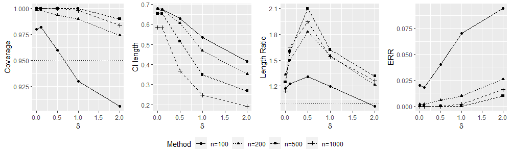
(a) setting6(a)

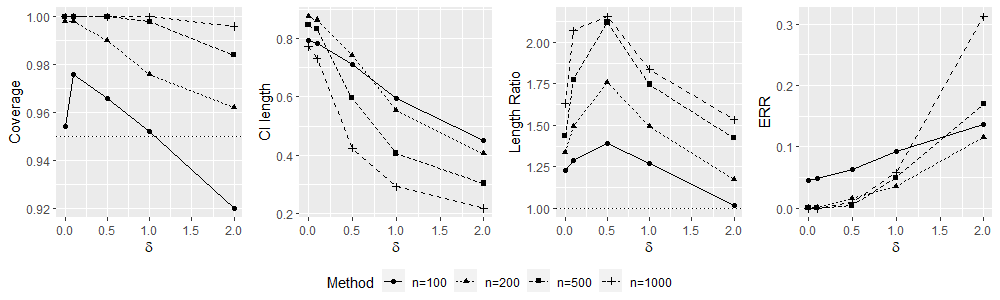
(b) setting6(b)

Figure S5: Setting 6 with opposite effects. “Coverage” and “CI Length” stand for the empirical coverage and the average length of our proposed CI, respectively; “Length Ratio” represents the ratio of the average length of our proposed CI to the normality CI in (33); “ERR” represents the empirical rejection rate out of 500 simulations.

G.2 Instability Measure: dependence on $\delta$

Recall the stability measure $\mathbb{I}(\delta)$ is introduced in Section 6 in the main paper,

$$\mathbb{I}(\delta)=\frac{\sum_{m=1}^{M}\|\widehat{\gamma}^{[m]}_{\delta}-\widehat{\gamma}_{\delta}\|^{2}_{2}}{\sum_{m=1}^{M}\|\widehat{\Gamma}^{[m]}-\widehat{\Gamma}^{\mathbb{Q}}\|^{2}_{2}},$$

where a larger $\mathbb{I}(\delta)$ indicates an unstable integration. In Table S2, we report the instability measure $\mathbb{I}(\delta)$ for all simulation settings except for setting 5, which is not included since it consists of more than 10 subsettings. We observe settings 1 and 6 are settings with instability. For both settings, the penalty $\delta$ is instrumental in decreasing the instability measure. For settings 2, 3, and 4, the small instability measure $\mathbb{I}(\delta)$ indicates that the standard maximin effect (without adding the ridge penalty) is already a stable integration.

setting	$L$	$\mathbb{I}(0)$	$\mathbb{I}(0.1)$	$\mathbb{I}(0.5)$	$\mathbb{I}(1)$	$\mathbb{I}(2)$	$\Gamma^{\mathbb{Q}}_{11}+\Gamma^{\mathbb{Q}}_{22}-2\Gamma^{\mathbb{Q}}_{12}$
1	2	5.464	1.966	0.264	0.072	0.019	0.026
2	2	0.023	0.021	0.014	0.010	0.006	4.635
3(a)	2	0.094	0.082	0.044	0.023	0.010	1.935
3(b)	2	0.058	0.050	0.029	0.017	0.008	2.810
4(a)	2	0.108	0.087	0.044	0.024	0.011	2.007
4(b)	5	0.076	0.059	0.027	0.014	0.006	-
4(c)	10	0.052	0.039	0.016	0.008	0.003	-
6(a)	2	3.305	1.449	0.221	0.065	0.018	0.160
6(b)	2	1.451	0.816	0.168	0.056	0.017	0.360

Table S2: The instability measure $\mathbb{I}(\delta)$ for $\delta\in\{0,0.1,0.5,1,2\}$. The reported values are averaged over 100 repeated simulations. For the column indexed with $\Gamma^{\mathbb{Q}}_{11}+\Gamma^{\mathbb{Q}}_{22}-2\Gamma^{\mathbb{Q}}_{12}$, we only report their values for $L=2$ since $\Gamma^{\mathbb{Q}}_{11}+\Gamma^{\mathbb{Q}}_{22}-2\Gamma^{\mathbb{Q}}_{12}$ is only a measure of instability for $L=2$.

G.3 Sample Splitting Comparison

We compare the algorithm with and without sample splitting and report the results in Table S3. For the sample splitting algorithm, we split the samples into two equal size sub-samples. For $n=100,$ no sample splitting algorithm is slightly under-coverage (the empirical coverage level is still above 90%). When $n\geq 200,$ both the algorithm with and without sample splitting achieve the desired coverage levels. As expected, the CIs with sample splitting are longer than those without sample splitting. In Table S3, under the column indexed with “Length ratio”, we report the ratio of the average length of CI with sample splitting to that without sample splitting.

		Coverage		Length
$\delta$	$n$	Splitting	No Splitting	Splitting	No Splitting	Length ratio
	100	0.978	0.920	1.921	1.062	1.809
	200	0.994	0.972	1.618	0.898	1.802
	300	0.994	0.990	1.336	0.789	1.693
0.0	500	1.000	0.992	0.999	0.651	1.534
	100	0.980	0.922	1.904	1.023	1.861
	200	0.994	0.972	1.567	0.863	1.816
	300	0.994	0.990	1.286	0.759	1.695
0.1	500	1.000	0.992	0.952	0.629	1.514
	100	0.982	0.918	1.814	0.890	2.038
	200	0.996	0.972	1.373	0.748	1.836
	300	0.996	0.992	1.099	0.666	1.651
0.5	500	1.000	0.994	0.800	0.559	1.433
	100	0.986	0.914	1.639	0.769	2.131
	200	0.998	0.968	1.155	0.655	1.764
	300	0.996	0.992	0.911	0.589	1.546
1.0	500	1.000	0.994	0.681	0.499	1.364
	100	0.986	0.902	1.291	0.630	2.049
	200	0.996	0.968	0.871	0.549	1.587
	300	0.998	0.988	0.706	0.499	1.415
2.0	500	0.998	0.992	0.549	0.426	1.290

Table S3: Comparison of algorithm with/without sample-splitting in setting 2 with $p=500.$

G.4 Additional results for real data analysis.

SNP index	420	423	424	437	442	443
Gene	KRE33	TCB2	IMP4	HPF1	SPO21	ATP19

Table S4: Gene names for several SNPs with maximin significant effects.

References

• D. W. Andrews (1999) Estimation when a parameter is on a boundary. Econometrica 67 (6), pp. 1341–1383. Cited by: §3.
• D. W. Andrews (2000) Inconsistency of the bootstrap when a parameter is on the boundary of the parameter space. Econometrica, pp. 399–405. Cited by: §3.
• M. Arjovsky, L. Bottou, I. Gulrajani, and D. Lopez-Paz (2019) Invariant risk minimization. arXiv preprint arXiv:1907.02893. Cited by: §1.3.
• S. Athey, G. W. Imbens, and S. Wager (2018) Approximate residual balancing: debiased inference of average treatment effects in high dimensions. Journal of the Royal Statistical Society: Series B (Statistical Methodology) 80 (4), pp. 597–623. Cited by: §1.3.
• A. Belloni, V. Chernozhukov, and C. Hansen (2014) High-dimensional methods and inference on structural and treatment effects. Journal of Economic Perspectives 28 (2), pp. 29–50. Cited by: §1.3.
• Y. Benjamini and Y. Hochberg (1995) Controlling the false discovery rate: a practical and powerful approach to multiple testing. Journal of the Royal statistical society: series B (Methodological) 57 (1), pp. 289–300. Cited by: §8.2.
• P. J. Bickel, Y. Ritov, and A. B. Tsybakov (2009) Simultaneous analysis of lasso and dantzig selector. The Annals of Statistics 37 (4), pp. 1705–1732. Cited by: §5.
• J. S. Bloom, I. M. Ehrenreich, W. T. Loo, T. V. Lite, and L. Kruglyak (2013) Finding the sources of missing heritability in a yeast cross. Nature 494 (7436), pp. 234–237. Cited by: §8.
• P. Bühlmann and N. Meinshausen (2015) Magging: maximin aggregation for inhomogeneous large-scale data. Proceedings of the IEEE 104 (1), pp. 126–135. Cited by: Figure 1, Figure 1, §1.3.
• P. Bühlmann and S. van de Geer (2011) Statistics for high-dimensional data: methods, theory and applications. Springer Science & Business Media. Cited by: §5.
• P. Bühlmann and S. van de Geer (2015) High-dimensional inference in misspecified linear models. Electronic Journal of Statistics 9 (1), pp. 1449–1473. Cited by: §9.
• T. T. Cai and Z. Guo (2017) Confidence intervals for high-dimensional linear regression: minimax rates and adaptivity. The Annals of Statistics 45 (2), pp. 615–646. Cited by: §1.3.
• T. T. Cai and Z. Guo (2020) Semisupervised inference for explained variance in high dimensional linear regression and its applications. Journal of the Royal Statistical Society Series B 82 (2), pp. 391–419. Cited by: §4.1.2.
• T. Cai, M. Liu, and Y. Xia (2021a) Individual data protected integrative regression analysis of high-dimensional heterogeneous data. Journal of the American Statistical Association, pp. 1–15. Cited by: §1.1.
• T. Cai, T. Tony Cai, and Z. Guo (2021b) Optimal statistical inference for individualized treatment effects in high-dimensional models. Journal of the Royal Statistical Society: Series B (Statistical Methodology) 83 (4), pp. 669–719. Cited by: §4.1.2, §4.1.2, §5.
• M. P. Calus and J. Vandenplas (2018) SNPrune: an efficient algorithm to prune large snp array and sequence datasets based on high linkage disequilibrium. Genetics Selection Evolution 50 (1), pp. 1–11. Cited by: §8.
• V. Chernozhukov, D. Chetverikov, M. Demirer, E. Duflo, C. Hansen, W. Newey, and J. Robins (2018) Double/debiased machine learning for treatment and structural parameters. The Econometrics Journal 21 (1), pp. C1–C68. Cited by: §1.3.
• V. Chernozhukov, C. Hansen, and M. Spindler (2015) Valid post-selection and post-regularization inference: an elementary, general approach. arXiv preprint arXiv:1501.03430. Cited by: §1.3.
• J. M. Cherry, E. L. Hong, C. Amundsen, R. Balakrishnan, G. Binkley, E. T. Chan, K. R. Christie, M. C. Costanzo, S. S. Dwight, S. R. Engel, et al. (2012) Saccharomyces genome database: the genomics resource of budding yeast. Nucleic acids research 40 (D1), pp. D700–D705. Cited by: §8.1.
• R. Dezeure, P. Bühlmann, and C. Zhang (2017) High-dimensional simultaneous inference with the bootstrap. Test 26 (4), pp. 685–719. Cited by: §8.
• E. Diana, W. Gill, M. Kearns, K. Kenthapadi, and A. Roth (2021) Minimax group fairness: algorithms and experiments. In Proceedings of the 2021 AAAI/ACM Conference on AI, Ethics, and Society, pp. 66–76. Cited by: §2.2.
• M. Drton (2009) Likelihood ratio tests and singularities. The Annals of Statistics 37 (2), pp. 979–1012. Cited by: §3.
• B. Efron (1979) Bootstrap methods: another look at the jackknife. The Annals of Statistics 7 (1), pp. 1–26. Cited by: §1.3.
• B. Efron and R. J. Tibshirani (1994) An introduction to the bootstrap. CRC press. Cited by: §1.3.
• M. H. Farrell (2015) Robust inference on average treatment effects with possibly more covariates than observations. Journal of Econometrics 189 (1), pp. 1–23. Cited by: §1.3.
• J. Friedman, T. Hastie, and R. Tibshirani (2010) Regularization paths for generalized linear models via coordinate descent. Journal of statistical software 33 (1), pp. 1. Cited by: §7.
• R. Gao, X. Chen, and A. J. Kleywegt (2017) Wasserstein distributional robustness and regularization in statistical learning. arXiv preprint arXiv:1712.06050. Cited by: §1.3, §2.2.
• Z. Guo, C. Renaux, P. Bühlmann, and T. T. Cai (2019) Group inference in high dimensions with applications to hierarchical testing. arXiv preprint arXiv:1909.01503. Cited by: §4.1.2.
• J. Hannig, H. Iyer, R. C. S. Lai, and T. C. M. Lee (2016) Generalized fiducial inference: a review and new results. Journal of American Statistical Association. Note: To appear. Accepted in March 2016. doidoi:10.1080/01621459.2016.1165102 Cited by: §1.3.
• W. Hu, G. Niu, I. Sato, and M. Sugiyama (2018) Does distributionally robust supervised learning give robust classifiers?. In International Conference on Machine Learning, pp. 2029–2037. Cited by: §1.3, §2.2.
• M. Humbert-Droz, P. Mukherjee, O. Gevaert, et al. (2022) Strategies to address the lack of labeled data for supervised machine learning training with electronic health records: case study for the extraction of symptoms from clinical notes. JMIR medical informatics 10 (3), pp. e32903. Cited by: §1.1, §2.1.
• M. E. Jakobsen and J. Peters (2022) Distributional robustness of k-class estimators and the pulse. The Econometrics Journal 25 (2), pp. 404–432. Cited by: §2.2.
• A. Javanmard and A. Montanari (2014) Confidence intervals and hypothesis testing for high-dimensional regression. The Journal of Machine Learning Research 15 (1), pp. 2869–2909. Cited by: §1.3, §5.
• K. L. Keys, A. C. Mak, M. J. White, W. L. Eckalbar, A. W. Dahl, J. Mefford, A. V. Mikhaylova, M. G. Contreras, J. R. Elhawary, C. Eng, et al. (2020) On the cross-population generalizability of gene expression prediction models. PLoS genetics 16 (8), pp. e1008927. Cited by: §1.1.
• P. Kraft, E. Zeggini, and J. P. Ioannidis (2009) Replication in genome-wide association studies. Statistical science: a review journal of the Institute of Mathematical Statistics 24 (4), pp. 561. Cited by: §1.1.
• S. Li, T. T. Cai, and H. Li (2020) Transfer learning for high-dimensional linear regression: prediction, estimation, and minimax optimality. arXiv preprint arXiv:2006.10593. Cited by: Remark 1.
• M. Liu, Y. Xia, T. Cai, and K. Cho (2020) Integrative high dimensional multiple testing with heterogeneity under data sharing constraints. arXiv preprint arXiv:2004.00816. Cited by: §1.3, Remark 1.
• N. Martinez, M. Bertran, and G. Sapiro (2020) Minimax pareto fairness: a multi objective perspective. In International Conference on Machine Learning, pp. 6755–6764. Cited by: §2.2.
• N. Meinshausen and P. Bühlmann (2015) Maximin effects in inhomogeneous large-scale data. The Annals of Statistics 43 (4), pp. 1801–1830. Cited by: Figure 1, Figure 1, §1.1, §1.1, §1.3, §2.2, §2.2, §2.3.
• S. J. Pan and Q. Yang (2009) A survey on transfer learning. IEEE Transactions on knowledge and data engineering 22 (10), pp. 1345–1359. Cited by: §1.1, §2.1.
• J. Peters, P. Bühlmann, and N. Meinshausen (2016) Causal inference by using invariant prediction: identification and confidence intervals. Journal of the Royal Statistical Society. Series B (Statistical Methodology), pp. 947–1012. Cited by: §1.3.
• D. N. Politis, J. P. Romano, and M. Wolf (1999) Subsampling. Springer Science & Business Media. Cited by: §1.3.
• P. Rakshit, T. T. Cai, and Z. Guo (2021) Sihr: an r package for statistical inference in high-dimensional linear and logistic regression models. arXiv preprint arXiv:2109.03365. Cited by: §7.
• L. Rasmy, Y. Wu, N. Wang, X. Geng, W. J. Zheng, F. Wang, H. Wu, H. Xu, and D. Zhi (2018) A study of generalizability of recurrent neural network-based predictive models for heart failure onset risk using a large and heterogeneous ehr data set. Journal of biomedical informatics 84, pp. 11–16. Cited by: §1.1.
• D. Rothenhäusler, N. Meinshausen, P. Bühlmann, and J. Peters (2018) Anchor regression: heterogeneous data meets causality. arXiv preprint arXiv:1801.06229. Cited by: §1.3, §2.2.
• D. Rothenhäusler, N. Meinshausen, and P. Bühlmann (2016) Confidence intervals for maximin effects in inhomogeneous large-scale data. In Statistical Analysis for High-Dimensional Data, pp. 255–277. Cited by: §1.3.
• S. Sagawa, P. W. Koh, T. B. Hashimoto, and P. Liang (2019) Distributionally robust neural networks for group shifts: on the importance of regularization for worst-case generalization. arXiv preprint arXiv:1911.08731. Cited by: §1.3, §2.2.
• S. G. Self and K. Liang (1987) Asymptotic properties of maximum likelihood estimators and likelihood ratio tests under nonstandard conditions. Journal of the American Statistical Association 82 (398), pp. 605–610. Cited by: §3.
• C. Shi, R. Song, W. Lu, and B. Fu (2018) Maximin projection learning for optimal treatment decision with heterogeneous individualized treatment effects. Journal of the Royal Statistical Society. Series B, Statistical methodology 80 (4), pp. 681. Cited by: §2.2, §2.3.
• H. Shimodaira (2000) Improving predictive inference under covariate shift by weighting the log-likelihood function. Journal of statistical planning and inference 90 (2), pp. 227–244. Cited by: Remark 2.
• H. Singh, V. Mhasawade, and R. Chunara (2021) Generalizability challenges of mortality risk prediction models: a retrospective analysis on a multi-center database. medRxiv. Cited by: §1.1.
• A. Sinha, H. Namkoong, R. Volpi, and J. Duchi (2017) Certifying some distributional robustness with principled adversarial training. arXiv preprint arXiv:1710.10571. Cited by: §1.3, §2.2.
• G. Sirugo, S. M. Williams, and S. A. Tishkoff (2019) The missing diversity in human genetic studies. Cell 177 (1), pp. 26–31. Cited by: §1.1.
• M. Sugiyama, M. Krauledat, and K. MÞller (2007) Covariate shift adaptation by importance weighted cross validation. Journal of Machine Learning Research 8 (May), pp. 985–1005. Cited by: Remark 2.
• Y. Tian and Y. Feng (2021) Transfer learning under high-dimensional generazed linear models. arXiv preprint arXiv:2105.14328. Cited by: Remark 1.
• R. Tibshirani (1996) Regression shrinkage and selection via the lasso. Journal of the Royal Statistical Society. Series B (Methodological) 58 (1), pp. 267–288. Cited by: §4.1.2.
• Y. Tsuboi, H. Kashima, S. Hido, S. Bickel, and M. Sugiyama (2009) Direct density ratio estimation for large-scale covariate shift adaptation. Journal of Information Processing 17, pp. 138–155. Cited by: Remark 2.
• S. van de Geer, P. Bühlmann, Y. Ritov, and R. Dezeure (2014) On asymptotically optimal confidence regions and tests for high-dimensional models. The Annals of Statistics 42 (3), pp. 1166–1202. Cited by: §1.3, §5.
• N. Verzelen and E. Gassiat (2018) Adaptive estimation of high-dimensional signal-to-noise ratios. Bernoulli 24 (4B), pp. 3683–3710. Cited by: §4.1.2.
• L. Wasserman (2014) Discussion:” a significance test for the lasso”. The Annals of Statistics 42 (2), pp. 501–508. Cited by: §9.
• M. Xie and K. Singh (2013) Confidence distribution, the frequentist distribution estimator of a parameter: a review. International Statistical Review 81 (1), pp. 3–39. Cited by: §1.3, §4.2.
• M. Xie and P. Wang (2022) Repro samples method for finite-and large-sample inferences. arXiv preprint arXiv:2206.06421. Cited by: §1.3.
• S. L. Zabell (1992) RA fisher and fiducial argument. Statistical Science 7 (3), pp. 369–387. Cited by: §1.3.
• C. Zhang and S. S. Zhang (2014) Confidence intervals for low dimensional parameters in high dimensional linear models. Journal of the Royal Statistical Society: Series B (Statistical Methodology) 76 (1), pp. 217–242. Cited by: §1.3, §5.
• R. Zhang and Y. Lin (2009) DEG 5.0, a database of essential genes in both prokaryotes and eukaryotes. Nucleic acids research 37 (suppl_1), pp. D455–D458. Cited by: §8.1.
• T. Zhao, G. Cheng, and H. Liu (2016) A partially linear framework for massive heterogeneous data. Annals of statistics 44 (4), pp. 1400. Cited by: §1.3, Remark 1.
• S. Zhou (2009) Restricted eigenvalue conditions on subgaussian random matrices. arXiv preprint arXiv:0912.4045. Cited by: §5.
• Y. Zhu and J. Bradic (2018) Linear hypothesis testing in dense high-dimensional linear models. Journal of the American Statistical Association, pp. 1–18. Cited by: §1.3.
• F. Zhuang, Z. Qi, K. Duan, D. Xi, Y. Zhu, H. Zhu, H. Xiong, and Q. He (2020) A comprehensive survey on transfer learning. Proceedings of the IEEE 109 (1), pp. 43–76. Cited by: §1.1, §2.1.

References

• D. W. Andrews (2000) Inconsistency of the bootstrap when a parameter is on the boundary of the parameter space. Econometrica, pp. 399–405. Cited by: §B.3.
• A. Belloni, V. Chernozhukov, and L. Wang (2011) Square-root lasso: pivotal recovery of sparse signals via conic programming. Biometrika 98 (4), pp. 791–806. Cited by: §A.3.
• P. J. Bickel, Y. Ritov, and A. B. Tsybakov (2009) Simultaneous analysis of lasso and dantzig selector. The Annals of Statistics 37 (4), pp. 1705–1732. Cited by: §C.4.
• P. Bühlmann and N. Meinshausen (2015) Magging: maximin aggregation for inhomogeneous large-scale data. Proceedings of the IEEE 104 (1), pp. 126–135. Cited by: §B.2.
• P. Bühlmann and S. van de Geer (2011) Statistics for high-dimensional data: methods, theory and applications. Springer Science & Business Media. Cited by: §C.4.
• T. T. Cai and Z. Guo (2020) Semisupervised inference for explained variance in high dimensional linear regression and its applications. Journal of the Royal Statistical Society Series B 82 (2), pp. 391–419. Cited by: §C.4.
• T. Cai, T. Tony Cai, and Z. Guo (2021) Optimal statistical inference for individualized treatment effects in high-dimensional models. Journal of the Royal Statistical Society: Series B (Statistical Methodology) 83 (4), pp. 669–719. Cited by: §C.5, Appendix E.
• T. Cai and W. Liu (2011) Adaptive thresholding for sparse covariance matrix estimation. Journal of the American Statistical Association 106 (494), pp. 672–684. Cited by: §F.2.2.
• E. Diana, W. Gill, M. Kearns, K. Kenthapadi, and A. Roth (2021) Minimax group fairness: algorithms and experiments. In Proceedings of the 2021 AAAI/ACM Conference on AI, Ethics, and Society, pp. 66–76. Cited by: §A.1.
• C. Dwork, M. Hardt, T. Pitassi, O. Reingold, and R. Zemel (2012) Fairness through awareness. In Proceedings of the 3rd innovations in theoretical computer science conference, pp. 214–226. Cited by: §A.1.
• J. Friedman, T. Hastie, and R. Tibshirani (2010) Regularization paths for generalized linear models via coordinate descent. Journal of statistical software 33 (1), pp. 1. Cited by: §A.3.
• N. Martinez, M. Bertran, and G. Sapiro (2020) Minimax pareto fairness: a multi objective perspective. In International Conference on Machine Learning, pp. 6755–6764. Cited by: §A.1.
• N. Meinshausen and P. Bühlmann (2015) Maximin effects in inhomogeneous large-scale data. The Annals of Statistics 43 (4), pp. 1801–1830. Cited by: §C.1.
• D. N. Politis, J. P. Romano, and M. Wolf (1999) Subsampling. Springer Science & Business Media. Cited by: §B.2.
• J. Rawls (2001) Justice as fairness: a restatement. Harvard University Press. Cited by: §A.1.
• D. Rothenhäusler, N. Meinshausen, and P. Bühlmann (2016) Confidence intervals for maximin effects in inhomogeneous large-scale data. In Statistical Analysis for High-Dimensional Data, pp. 255–277. Cited by: §B.2, §B.2, §B.2.
• C. Shi, R. Song, W. Lu, and B. Fu (2018) Maximin projection learning for optimal treatment decision with heterogeneous individualized treatment effects. Journal of the Royal Statistical Society. Series B, Statistical methodology 80 (4), pp. 681. Cited by: §A.2, §A.2, §A.2.
• T. Sun and C. Zhang (2012) Scaled sparse linear regression. Biometrika 101 (2), pp. 269–284. Cited by: §A.3, §C.4.
• R. Tibshirani (1996) Regression shrinkage and selection via the lasso. Journal of the Royal Statistical Society. Series B (Methodological) 58 (1), pp. 267–288. Cited by: §A.3.
• R. Vershynin (2012) Introduction to the non-asymptotic analysis of random matrices. In Compressed Sensing: Theory and Applications, Y. Eldar and G. Kutyniok (Eds.), pp. 210–268. Cited by: §C.4, §F.2.2.
• F. Ye and C. Zhang (2010) Rate minimaxity of the lasso and dantzig selector for the $\ell_{q}$ loss in $\ell_{r}$ balls. The Journal of Machine Learning Research 11, pp. 3519–3540. Cited by: §C.4.
• S. Zhou (2009) Restricted eigenvalue conditions on subgaussian random matrices. arXiv preprint arXiv:0912.4045. Cited by: §C.4.