Networked Multi-Virus Spread with a Shared Resource: Analysis and Mitigation Strategies

Abstract

The paper studies multi-competitive continuous-time epidemic processes in the presence of a shared resource. We consider the setting where multiple viruses are simultaneously prevalent in the population, and the spread occurs due to not only individual-to-individual interaction but also due to individual-to-resource interaction. In such a setting, an individual is either not affected by any of the viruses, or infected by one and exactly one of the multiple viruses. We classify the equilibria into three classes: a) the healthy state (all viruses are eradicated), b) single-virus endemic equilibria (all but one viruses are eradicated), and c) coexisting equilibria (multiple viruses simultaneously infect separate fractions of the population). We provide i) a sufficient condition for exponential (resp. asymptotic) eradication of a virus; ii) a sufficient condition for the existence, uniqueness and asymptotic stability of a single-virus endemic equilibrium; iii) a necessary and sufficient condition for the healthy state to be the unique equilibrium; and iv) for the bi-virus setting (i.e., two competing viruses), a sufficient condition and a necessary condition for the existence of a coexisting equilibrium. Building on these analytical results, we provide two mitigation strategies: a technique that guarantees convergence to the healthy state; and, in a bi-virus setup, a scheme that employs one virus to ensure that the other virus is eradicated. The results are illustrated in a numerical study of a spread scenario in Stockholm city.

I Introduction

In February $1918$ a deadly influenza pandemic (popularly known as the Spanish flu) swept across the globe. It lasted until $1920$, and caused approximately $50$ million deaths [1]. Influenza viruses have continued to spread across the globe in recurring epidemics [2]. Given that the spread of infectious diseases has an enormous impact on society, the study of spread has been an active area of research since Bernoulli’s seminal paper [3]. The overarching goal of these research directions is to find conditions that would cause an epidemic to become eradicated, and leverage the knowledge of these conditions to design spread control strategies. To this end, various infection models have been proposed and studied in the literature; susceptible-infected-susceptible (SIS), susceptible-infected-removed (SIR), susceptible-exposed-infected-removed (SEIR), etc. In this paper, we focus on SIS models.

More specifically, we consider networked SIS models, in which a population of individuals is divided into subpopulations, and the infection can spread both within and between these subpopulations. Networked SIS models have been studied extensively using discrete-time [4, 5, 6, 7] and continuous-time dynamics [8, 9, 10]. In the present paper, we will focus on continuous-time dynamics. Although both time-invariant and time-varying continuous-time models have been studied in the literature (see for instance [11, 12] and references therein), we will restrict ourselves to the time-invariant case.

The spread represented by the SIS model has typically been understood as a consequence of human contact. However, the spread of infectious diseases can significantly worsen due to the presence of a shared resource. For example, waterborne pathogens spread via water distribution systems [13] and droplet-transmitted pathogens spread via surfaces in public transit vehicles [14]. Such observations have motivated the development of the susceptible-infected-water-susceptible (SIWS) model [15, 16] – essentially, a networked continuous-time single-virus SIS model that incorporates shared resources. For the SIWS model with a single shared resource, sufficient conditions for asymptotic convergence to the healthy state (where each subpopulation is infection-free, and the shared resource is contamination-free) have been provided [15, Theorem 1]. This result has been generalized to also account for multiple shared resources in [16, Theorem 1], where virus transmission could be due to individual-to-individual contact, due to individual-to-resource contact, and, in contrast to the single resource case, also due to resource-to-resource contact. However, no theoretical guarantees for the endemic behavior (i.e., where the virus persists) of the SIWS model have been provided.

The analysis of epidemic spread using SIWS models has been restricted to the single-virus case. While such analysis provides insights into how to battle an epidemic, they do not account for settings where multiple strains of a virus could be simultaneously active within a population. In particular, it is possible that viral strains compete with each other to infect the population: each individual can be infected by one, and only one, of the multiple viral strains prevalent [17], i.e., the strains impose cross-immunity. Such a phenomenon is not only restricted to epidemics, but may also appear in the context of incompatible information transmission on social networks [18], or of two competing products within the same market [19]. It is well-known that competitive multi-virus propagation exhibits rich behaviour in comparison to single-virus propagation [20]. One possible outcome of competitive multi-virus propagation is coexistence (i.e., multiple strains coexist in a population by infecting separate fractions of each subpopulation), while another is competitive exclusion (i.e., the spread parameters of one strain dominate those of the other strains, thereby causing those strains to become eradicated). In particular, [21] established that cross-immunity between strains typically leads to competitive exclusion in single-population SIS models, whereas [22, 23, 24, 18] provided conditions for coexistence in networked SIS models. In particular, analysis of the various equilibria of a competing continuous-time time-invariant bi-virus model has been provided in [23], whereas a necessary and sufficient condition for a coexisting equilibrium has been established [24, Theorem 6]. However, the results obtained in [23, 24] are restrictive in the following sense: i) [23, Theorems 6 and 7] rely on the assumption that the spread parameters with respect to each virus is the same for every subpopulation; and ii) [24, Theorem 6] is reliant on the assumption that the set of spread parameters for each virus is a scaled version of that of other viruses. Moreover, none of these works account for the presence of a shared resource in the network. Thus, to the best of our knowledge, for the multi-virus SIWS model, a detailed analysis of the various equilibria and their stability properties remains missing in the literature. The present paper aims to fill this gap and in the process, for bi-virus SIS models, establish conditions for the existence of a coexisting equilibrium under less stringent assumptions.

The overarching goal is to develop strategies for the eradication of epidemics. Several control strategies have been formulated in the context of networked SIS models: optimal antidote distribution [25], contact reduction [26, 27], etc. In particular, for a directed network with heterogeneous spread, [28] provides a fully distributed Alternating Direction Method of Multipliers (ADMM) algorithm that allows for local computation of optimal investment required to boost the healing rate at each node. Note that this ADMM algorithm requires every node to communicate with its neighbors its local estimate of the full network, which can be undesirable to do in practice. A decentralized algorithm that involves disconnecting nodes and increasing the healing rates, subject to resource constraints, has been proposed in [29]. More recently, a distributed algorithm that, given resource limitations, guarantees the eradication of an epidemic with a specified rate has been proposed in [25]. In the case of multiple cross-immune strains, eradication of all viruses via optimal antidote distribution is featured in [30]. In certain multi-strain epidemics, one strain can impose more severe symptoms than other strains [31]. If resource limitations do not permit us to eradicate all strains, we might prioritize eradicating a malignant strain first. The idea of eradicating one strain while sustaining another has been explored in [32]. Note that the algorithms provided in [23, 28, 29, 25], and the results in [33, 24, 32, 34] account only for SIS models.

Paper Contributions

The paper studies the multi-virus SIWS model. We establish existence, uniqueness and stability of certain equilibria, and develop mitigation strategies based on these results, as follows:

1. Since the persistence of a virus has an enormous impact on society, it is important to know under what conditions a virus persists and, assuming at least one individual in a subpopulation is infected initially, if the virus can become endemic in the population. To this end, we provide a sufficient condition for the existence, uniqueness, and asymptotic stability of a single-virus endemic equilibrium; see Theorem 3.

2. In the bi-virus case with (resp. without) a shared resource, as discussed previously, a natural question is whether both viruses can persist simultaneously. We establish a sufficient condition for the existence of a coexisting equilibrium; see Theorem 5 (resp. Corollary 1).

3. Similarly, in the bi-virus case with (resp. without) a shared resource, it is also important to determine conditions that lead to competitive exclusion. Thus, we establish a necessary condition for the existence of a coexisting equilibrium; see Theorem 6 (resp. Corollary 2).

4. Utilizing our analytical results, we have developed two mitigation strategies: one for the stabilization (exponential or asymptotic) of the healthy state, and the other for the eradication of a malignant virus in the bi-virus case; see Theorems 7 and 8, respectively.

Additionally, we present results on the stability and uniqueness of the healthy state, see Theorems 1, 2 and 4. A preliminary version of some of the results in this paper is scheduled for presentation at the $3^{\rm{rd}}$ IFAC Workshop on Cyber-Physical & Human Systems; see [35].

The aforementioned findings have several consequences. In an epidemiological context, the results on the healthy state shed light on the conditions that ensure the eradication of a virus in the population and the shared resource, and, therefore, aid in developing a mitigation strategy (see Section VII). The results on the single-virus endemic equilibrium are useful for learning the spread parameters (i.e., healing rate and infection rate), as discussed for the special case of SIS models in [36]. One of the results concerning the coexisting equilibrium inspires a novel virus eradication strategy, where the goal is to push the dynamics towards the single-virus endemic equilibrium of the benign virus, as opposed to the healthy state (see Section VII). The results on the existence of a coexisting equilibrium find applications not just in epidemiology, but also in opinion dynamics in social networks, where it provides conditions under which competing ideas (for instance, pro-Covid-19 restrictions versus anti-Covid-19 restrictions) coexist in different groups of the same population.

Paper Outline

The paper is organized as follows: We introduce the model and formally present the main problems being investigated in Section II. We collect the necessary technical background needed for establishing our main results in Section III. The main results are split up across Sections IV–VII. More specifically, Sections IV–VI concern the analysis of equilibria, whereas mitigation strategies for eradicating or mitigating the spread of viruses are provided in Section VII. We illustrate our findings via simulations in Section VIII. Finally, we summarize the main findings of our paper, and highlight relevant problems of future interest in Section IX.

Notations

We denote the set of real numbers by $\mathbb{R}$, and the set of nonnegative real numbers by $\mathbb{R}_{+}$. For any positive integer $n$, we use $[n]$ to denote the set $\{1,2,...,n\}$. The $i^{\rm{th}}$ entry of a vector $x$ is denoted by $x_{i}$. The element in the $i^{\rm{th}}$ row and $j^{\rm{th}}$ column of a matrix $M$ is denoted by $M_{ij}$. We use 0 and 1 to denote the vectors whose entries all equal $0$ and $1$, respectively, and use $I$ to denote the identity matrix, while the sizes of the vectors and matrices are to be understood from the context. For a vector $x$ we denote the square matrix with $x$ along the diagonal by $\operatorname{diag}(x)$. For any two real vectors $a,b\in\mathbb{R}^{n}$ we write $a\geq b$ if $a_{i}\geq b_{i}$ for all $i\in[n]$, $a>b$ if $a\geq b$ and $a\neq b$, and $a\gg b$ if $a_{i}>b_{i}$ for all $i\in[n]$. Likewise, for any two real matrices $A,B\in\mathbb{R}^{n\times m}$, we write $A\geq B$ if $A_{ij}\geq B_{ij}$ for all $i\in[n]$, $j\in[m]$, and $A>B$ if $A\geq B$ and $A\neq B$. For a square matrix $M$, we use $\sigma(M)$ to denote the spectrum of $M$, $\rho(M)$ to denote the spectral radius of $M$, and $s(M)$ to denote the largest real part among the eigenvalues of $M$, i.e., $s(M)=\max\{\rm{Re}(\lambda):\lambda\in\sigma(M)\}$. Given a matrix $A$, $A\prec 0$ (resp. $A\preccurlyeq 0$) indicates that $A$ is negative definite (resp. negative semidefinite), whereas $A\succ 0$ (resp. $A\succcurlyeq 0$) indicates that $A$ is positive definite (resp. positive semidefinite). We denote a subset by $P\subseteq Q$, a proper subset by $P\subset Q$, and set difference by $P\setminus Q$.

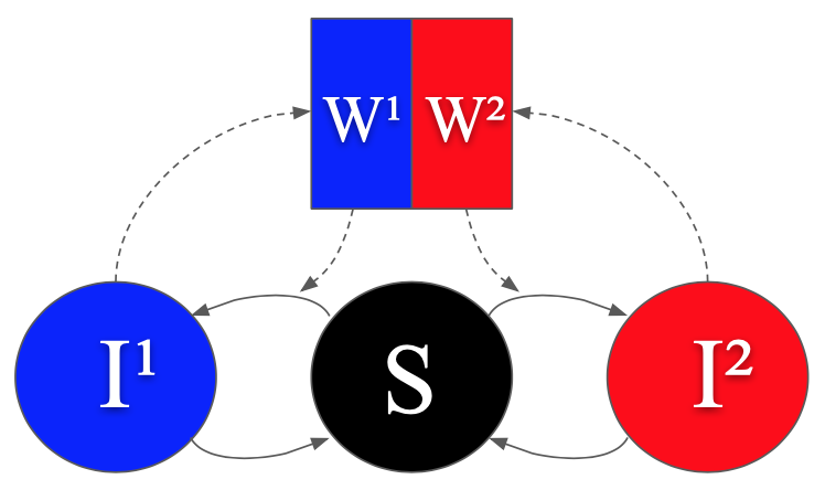
Figure 1: Visualization of the model for the case when $m=2$. An individual is either susceptible (S), infected with virus $1$ (I¹), or infected with virus $2$ (I²). The shared resource (W) is contaminated by individuals infected with either virus, and in turn augments the corresponding infection rate.

II Problem Formulation

In this section, we detail a model of multi-viral spread across a population network with a shared resource. We then formally state the problems being investigated. Finally, we introduce pertinent assumptions and definitions for use in later sections.

II-A The multi-virus SIWS model

Consider a population of individuals, subdivided into $n$ population nodes in a network, with a resource $W$ being shared among some or all of the population nodes. Suppose that $m$ viruses are active in the population. An individual can become infected by a virus, either by coming into contact with an infected individual, or due to interaction with the (possibly) contaminated shared resource. We make the assumption that viral infection causes cross-immunity, meaning that an individual can be infected by no more than one virus at the same time. An infected individual can then recover, returning to the susceptible state. The model is visualized from an individual’s perspective in Figure 1. The spread of the $m$ viruses across the population can be represented by a multi-layer network $G$ with $m$ layers, where the vertices correspond to population nodes and the shared resource, and each layer contains a set of directed edges, $E^{k}$, specific to each virus $k$. There exists a directed edge from node $j$ to node $i$ in $E^{k}$ if an individual, infected by virus $k$ in node $j$, can directly infect individuals in node $i$. Furthermore, the existence of a directed edge in $E^{k}$ from node $j$ (resp. from the shared resource $W$) to the shared resource $W$ (resp. to the node $j$) signifies that the shared resource $W$ (resp. node $j$) can be contaminated with virus $k$ by infected individuals in node $j$ (resp. by the shared resource $W$). We say that the $k^{\rm{th}}$ layer of $G$ is strongly connected if there is a path via the directed edges in $E^{k}$ from each node, and from the shared resource, to every node, and to the shared resource. In real-world scenarios, it is often the case that viral epidemics can spread from each subpopulation to every other subpopulation, in which case we assume that each layer is strongly connected.

Each population node $i$ contains $N_{i}$ individuals, with a birth rate $\mu_{i}$ equal to its death rate $\bar{\mu}_{i}$. At any time $t\geq 0$, $S_{i}(t)$ is the number of susceptible individuals in node $i$, while $I_{i}^{k}(t)$ is the number of individuals infected by virus $k$ in node $i$, while $S_{i}(t)+\textstyle\sum_{k=1}^{m}I_{i}^{k}(t)=N_{i}$. The rate at which individuals infected by virus $k$ in node $j$ infect susceptible individuals in node $i$ is denoted by $\alpha_{ij}^{k}$, where $\alpha_{ij}^{k}=0$ corresponds to the absence of a directed edge from node $j$ to node $i$ in $E^{k}$. In node $i$, individuals infected by virus $k$ recover to the susceptible state at a rate $\gamma_{i}^{k}$. The shared resource contains a viral mass with respect to each virus $k$, denoted by $W^{k}(t)$, representing the level of contamination at time $t\geq 0$. The viral mass of virus $k$ grows at a rate proportional to all $I_{i}^{k}(t)$ scaled by their corresponding rates $\zeta_{i}^{k}$, and decays at a rate $\delta_{w}^{k}$. The resource-to-node infection rate to node $i$ with respect to virus $k$ is denoted by $\alpha_{iw}^{k}$. The time evolution of the number of susceptible and infected individuals (with respect to each virus $k\in[m]$) in population node $i\in[n]$ is given by

$$\begin{split}\dot{S}_{i}(t)=&\,\mu_{i}N_{i}-\bar{\mu}_{i}S_{i}(t)+\textstyle\sum_{k=1}^{m}\gamma_{i}^{k}I_{i}^{k}(t)\\ &-\textstyle\sum_{k=1}^{m}\big{(}\alpha_{iw}^{k}W^{k}(t)-\textstyle\sum_{j=1}^{n}\alpha_{ij}^{k}\frac{I_{j}^{k}(t)}{N_{i}}\big{)}S_{i}(t),\\ \dot{I}_{i}^{k}(t)=&-\,(\bar{\mu}_{i}+\gamma_{i}^{k})I_{i}^{k}(t)\\ &+\big{(}\alpha_{iw}^{k}W^{k}(t)+\textstyle\sum_{j=1}^{n}\alpha_{ij}^{k}\frac{I_{j}^{k}(t)}{N_{i}}\big{)}S_{i}(t),\\ \dot{W}^{k}(t)=&-\delta_{w}^{k}W^{k}(t)+\textstyle\sum_{j=1}^{n}\zeta_{j}^{k}I_{j}^{k}(t).\end{split}$$ (1)

We define new variables to simplify the system. Let

$$p_{i}^{k}(t)\coloneqq\frac{I_{i}^{k}(t)}{N_{i}},\,z^{k}(t)\coloneqq\frac{\delta_{w}^{k}W^{k}(t)}{\sum_{j=1}^{n}\zeta_{j}^{k}N_{j}},\,\delta_{i}^{k}\coloneqq\gamma_{i}^{k}+\mu_{i},$$

$$\beta_{ij}^{k}\coloneqq\alpha_{ij}^{k}\frac{N_{j}}{N_{i}},\,\beta_{iw}^{k}\coloneqq\frac{\alpha_{iw}^{k}}{\delta_{w}^{k}}\textstyle\sum_{j=1}^{n}\zeta_{j}^{k}N_{j},c_{i}^{k}\coloneqq\frac{\zeta_{i}N_{i}}{\sum_{j=1}^{n}\zeta_{j}^{k}N_{j}},$$

where the variables can be interpreted as follows: With respect to virus $k$, $p_{i}^{k}(t)$ is the fraction of currently infected individuals in node $i$, $z^{k}(t)$ is a scaled contamination level in the shared resource, $\delta_{i}^{k}$ is the healing rate in node $i$, $\beta_{ij}^{k}$ is the node-to-node infection rate from node $j$ to $i$, scaled with respect to population ratios, $\beta_{iw}^{k}$ is a scaled resource-to-node infection rate to node $i$, and $c_{i}^{k}$ is a scaled node-to-resource contamination rate from node $i$. Then, assuming that the birth rates and death rates are equal for each node, (1) can be rewritten as

$$\dot{p}_{i}^{k}(t)=-\delta_{i}^{k}p_{i}^{k}(t)+\big{(} 1-\textstyle\sum_{l=1}^{m}p_{i}^{l}(t)\big{)}$$

$$\times\big{(}\beta_{iw}^{k}z^{k}(t)+\textstyle\sum_{j=1}^{n}\beta_{ij}^{k}p_{j}^{k}(t)\big{)},$$

$$\dot{z}^{k}(t)=\delta_{w}^{k}\big{(}-z^{k}(t)+ \textstyle\sum_{i=1}^{n}c_{i}^{k}p_{i}^{k}(t)\big{)}.$$ (2)

Using vector notation, (2) can be rewritten as

$$\begin{split}\dot{p}^{k}(t)=&\,\Big{(}\big{(}I-\textstyle\sum_{l=1}^{m}\operatorname{diag}(p^{l}(t))\big{)}B^{k}-D^{k}\Big{)}p^{k}(t)\\ &\,\,+\big{(}I-\textstyle\sum_{l=1}^{m}\operatorname{diag}(p^{l}(t))\big{)}b^{k}z^{k}(t),\\ \dot{z}^{k}(t)=&\,\delta_{w}^{k}\big{(}-z^{k}(t)+c^{k}p^{k}(t)\big{)},\\ \end{split}$$ (3)

where $B^{k}$ is an $n\times n$-matrix with $\beta_{ij}^{k}$ as the $(i,j)^{\rm{th}}$ element, $D^{k}$ is a diagonal $n\times n$-matrix with $D_{ii}^{k}=\delta_{i}^{k}$ for all $i\in[n]$, $b^{k}$ is a column vector with $\beta_{iw}^{k}$ as the $i^{\rm{th}}$ element, and $c^{k}$ is a row vector with $c_{i}^{k}$ as the $i^{\rm{th}}$ element. To simplify notation further, we define

$$y^{k}(t)\coloneqq\begin{bmatrix}p^{k}(t)\\ z^{k}(t)\end{bmatrix},y(t)\coloneqq\begin{bmatrix}y^{1}(t)\\ \vdots\\ y^{m}(t)\\ \end{bmatrix},\normalsize B_{w}^{k}\coloneqq\begin{bmatrix}B^{k}&b^{k}\\ \delta_{w}^{k}c^{k}&0\end{bmatrix},$$

$$X(y^{k}(t))\coloneqq\begin{bmatrix}\operatorname{diag}(p^{k}(t))&0\\ 0&0\end{bmatrix},\,\,D_{w}^{k}\coloneqq\begin{bmatrix}D^{k}&0\\ 0&\delta_{w}^{k}\end{bmatrix}.$$

With these variables in place, we can rewrite (3) as

$$\dot{y}^{k}(t)=\big{(}-D_{w}^{k}+(I-\textstyle\sum_{l=1}^{m}X(y^{l}(t)))B_{w}^{k}\big{)}y^{k}(t).$$ (4)

Defining $A_{w}^{k}(y(t))\coloneqq\big{(}-D_{w}^{k}+(I-\textstyle\sum_{l=1}^{m}X(y^{l}(t)))B_{w}^{k}\big{)}$, the dynamics of the system of all $m$ viruses are given by

$$\dot{y}(t)=\begin{bmatrix}A_{w}^{1}\big{(}y(t)\big{)}&0&\dots&0\\ 0&A_{w}^{2}\big{(}y(t)\big{)}&\dots&0\\ \vdots&\vdots&\ddots&\vdots\\ 0&0&\dots&A_{w}^{m}\big{(}y(t)\big{)}\end{bmatrix}y(t).$$ (5)

We say that virus $k\in[m]$ is eradicated, or in its eradicated state, if $y^{k}=\textbf{0}$, which is clearly an equilibrium of (4). When considering the system of $m$ viruses (5), we say that the system is in the healthy state if all viruses are eradicated, i.e., $y=\textbf{0}$. If (5) has an endemic (non-zero) equilibrium, it can belong to one of two types: single-virus endemic equilibrium, where $y^{k}>\textbf{0}$ for some $k\in[m]$ and all other viruses in $[m]$ are eradicated; or coexisting equilibrium, where $y^{k}>\textbf{0}$ for multiple $k\in[m]$.

II-B Problem Statements

For the model (5), we formally state the problems being investigated in this paper.

1. Under what conditions does $y^{k}(t)$ converge exponentially, or asymptotically, to its eradicated state, i.e., $y^{k}=\textbf{0}$, for some $k\in[m]$?

2. For a single-virus setup, i.e., $m=1$, under what conditions does the system have a unique single-virus endemic equilibrium, $y^{*}>\textbf{0}$, and under such conditions, does the system converge asymptotically to $y^{*}$ from any non-zero initial condition?

3. What is a necessary and sufficient condition for the healthy state, i.e., $y=\textbf{0}$, to be the unique equilibrium?

4. For a bi-virus setup, i.e., $m=2$, under what conditions does the system have a coexisting equilibrium, i.e., $(\hat{y}^{1},\hat{y}^{2})$ such that $\hat{y}^{1}>\textbf{0}$ and $\hat{y}^{2}>\textbf{0}$?

5. For a bi-virus setup, under what conditions does the system not have a coexisting equilibrium, i.e., $(\hat{y}^{1},\hat{y}^{2})$ such that $\hat{y}^{1}>\textbf{0}$ and $\hat{y}^{2}>\textbf{0}$?

6. How can the healing rates, i.e., $\delta_{i}^{k}$, be chosen to ensure that the system converges exponentially, or asymptotically, to the healthy state, i.e., $y=\textbf{0}$?

7. For a bi-virus setup, how can the healing rates of virus $2$, i.e., $\delta_{i}^{2}$, be chosen to ensure that the system converges to the single-virus endemic equilibrium of virus $1$?

Before we address these questions, we point out two connections between the considered setup and the existing literature.

Remark 1.

If $m=1$, system (4) coincides with the single-virus model proposed in [15] $\blacksquare$

Hereafter, when a single-virus system is considered, we drop the superscripts identifying the virus from all variables:

$B_{w}\coloneqq B_{w}^{1}$, $D_{w}\coloneqq D_{w}^{1}$, etc.

Remark 2.

Note that if $b^{k}=\textbf{0}$ for all $k\in[m],$ the influence of the shared resource on the population is nullified. Then, the multi-virus dynamics of the population nodes, $p^{k}(t)$, in (5) are equivalent to the time-invariant multi-virus setup of [30]. $\blacksquare$

II-C Positivity assumptions

In order for (5) to be well-defined and realistic, we make the following assumption.

Assumption 1.

Suppose that $\delta_{i}^{k}>0,\delta_{w}^{k}>0,\beta_{ij}^{k}\geq 0,\beta_{iw}^{k}\geq 0$ and $c_{i}^{k}\geq 0$ for all $i,j\in[n]$ and $k\in[m]$, with $c_{l}^{k}>0$ for at least one $l\in[n]$. $\blacksquare$

Note that if Assumption 1 holds, then for all $k\in[m]$, $B_{w}^{k}$ is a nonnegative matrix and $D_{w}^{k}$ is a positive diagonal matrix Moreover, recall that a square matrix $M$ is said to be irreducible if, replacing the non-zero elements of $M$ with ones and interpreting it as an adjacency matrix, the corresponding graph is strongly connected. Then, noting that non-zero elements in $B_{w}^{k}$ represent directed edges in the set $E^{k}$, we see that $B_{w}^{k}$ is irreducible whenever the $k^{\rm{th}}$ layer of the multi-layer network $G$ is strongly connected.

Thanks to Assumption 1, we can restrict our analysis to the sets $\mathcal{D}\coloneqq\{y(t):p^{k}(t)\in[0,1]^{n},z^{k}(t)\in[0,\infty)\,\forall k\in[m]\}$ and $\mathcal{D}^{k}\coloneqq\{y^{k}(t):p^{k}(t)\in[0,1]^{n},\,z^{k}(t)\in[0,\infty)\}$. Since $p_{i}^{k}(t)$ is to be interpreted as a fraction of a population, and $z^{k}(t)$ is a nonnegative quantity, these sets represent the sensible domain of the system. That is, if $y^{k}(t)$ takes values outside of $\mathcal{D}^{k}$, then those values would lack physical meaning. The following lemma shows that once $y(t)$ enters $\mathcal{D}$, it never leaves $\mathcal{D}$.

Lemma 1.

Let Assumption 1 hold. Then $\mathcal{D}$ is positively invariant with respect to (5) $\blacksquare$

Proof: Consider $y(t)\in\mathcal{D}$. If $p_{i}^{k}(t)=1$, then $\dot{p}_{i}^{k}(t)<0$, so if $p_{i}^{k}(0)\leq 1$ then $p_{i}^{k}(t)\leq 1$, for all $t\geq 0$, $k\in[m],i\in[n]$. Further, if $p_{i}^{k}(t)=0$ and $y(t)\geq\textbf{0}$, then $\dot{p}_{i}^{k}(t)\geq 0$, for all $t\geq 0$. Similarly, if $z^{k}(t)=0$ and $y(t)\geq\textbf{0}$, then $\dot{z}^{k}(t)\geq 0$. Thus, $y(t)\geq\textbf{0}$ if $y(0)\geq\textbf{0}$, for all $t\geq 0$. $\square$

III Preliminaries

In this section, we recall some preliminary results, pertinent to the analysis of system (5). A real square matrix is said to be Metzler if all elements outside the diagonal are nonnegative. We require the following results for Metzler matrices.

Lemma 2.

[9, Lemma A.1] Suppose that $M$ is an irreducible Metzler matrix such that $s(M)=0$. Then there exists a positive diagonal matrix $P$ such that $M^{T}P+PM\preccurlyeq 0$. $\blacksquare$

Lemma 3.

[23, Proposition 1] Suppose that $\Lambda$ is a negative diagonal matrix and $N$ is an irreducible nonnegative matrix. Let $M$ be the irreducible Metzler matrix $M=\Lambda+N$. Then, $s(M)<0$ if and only if $\rho(-\Lambda^{-1}N)<1,s(M)=0$ if and only if $\rho(-\Lambda^{-1}N)=1$, and $s(M)>0$ if and only if, $\rho(-\Lambda^{-1}N)>1$. $\blacksquare$

We will also be making use of the following variants of the Perron-Frobenius theorem for irreducible matrices.

Lemma 4.

[37, Chapter 8.3] [38, Theorem 2.7] Suppose that $N$ is an irreducible nonnegative matrix. Then,

1. $r=\rho(N)$ is a simple eigenvalue of $N$.

2. There is an eigenvector $\zeta\gg\textbf{0}$ corresponding to the eigenvalue $r$.

3. $x>\textbf{0}$ is an eigenvector of $N$ only if $Nx=rx$ and $x\gg\textbf{0}$.

4. If $A$ is a nonnegative matrix such that $A<N$, then $\rho(A)<\rho(N)$.  $\blacksquare$

Lemma 5.

[38, Lemma 2.3] Suppose that $M$ is an irreducible Metzler matrix. Then $r=s(M)$ is a simple eigenvalue of $M$, and a corresponding eigenvector is $\zeta\gg\textbf{0}$. $\blacksquare$

Let $\mathbb{G}\subseteq\mathbb{R}^{n}$. Consider

$$\dot{x}(t)=f(x),$$ (6)

where $f:\mathbb{G}\rightarrow\mathbb{R}^{n}$ is a locally Lipschitz map.

Proposition 1.

Let 0 be an equilibrium of (6) and $\mathbb{E}\subseteq\mathbb{G}$ be a positively invariant and connected set with respect to (6), containing 0. Let $V:\mathbb{E}\rightarrow\mathbb{R}$ be a continuously differentiable and positive definite function, such that $\dot{V}(x(t))$ is negative definite. Further, let it hold that

$$\{x:V(x)\leq c\}\cap\mathbb{E}$$ (7)

is a bounded set for any constant $c>0$, and is equal to $\mathbb{E}$ as $c\rightarrow\infty$. Then the equilibrium 0 is asymptotically stable, with domain of attraction containing $\mathbb{E}$. $\blacksquare$

This proposition can be proven using [39, Theorem 4.1]. The following lemma pertains to system (5), providing a constraint on any endemic equilibrium.

Lemma 6.

Consider system (5) under Assumption 1. Suppose, for all $k\in[m]$, that $B_{w}^{k}$ is irreducible. If $y=(y^{1},\dots,y^{m})\in\mathcal{D}$ is an equilibrium of (5), then, for each $k\in[m]$, either $y^{k}=\textbf{0}$, or $\textbf{0}\ll y^{k}\ll\textbf{1}$. Moreover, $\textstyle\sum_{k=1}^{m}y^{k}\ll\textbf{1}$. $\blacksquare$

Proof: See Appendix. $\square$

Lemma 6 states that when the underlying network is strongly connected, any endemic equilibrium involves each active virus infecting a separate fraction of each population node, and contaminating the shared resource to some degree.

IV Analysis of the eradicated state of a virus

In this section, we present sufficient conditions for the exponential (resp. asymptotic) stability of the eradicated state of a virus. The key condition is found through eigenvalue analysis of $(B_{w}^{k}-D_{w}^{k})$, as seen in the following theorem.

Theorem 1.

Consider the SIWS model (4) under Assumption 1 with $y(0)\in\mathcal{D}$. Suppose that for some virus $k\in[m]$ we have $s(B_{w}^{k}-D_{w}^{k})<0$. Then the eradicated state of virus $k$ is exponentially stable, with domain of attraction containing $\mathcal{D}^{k}$. $\blacksquare$

Proof: See Appendix. $\square$

Theorem 1 states that if the linearized state matrix of virus $k$ is Hurwitz, then, for all initial conditions in the sensible domain, virus $k$ is eradicated exponentially fast. Theorem 1 answers the first part of question (i) in Section II-B. With respect to [23, Proposition 2], Theorem 1 is an improvement in the sense that it holds globally (on the sensible domain), and accounts for the multi-virus case, whereas [23, Proposition 2] established local exponential stability for the single-virus case.

Theorem 1 indeed guarantees exponential eradication of virus $k$, however, the condition is quite strict. For certain viruses it suffices to know whether or not the virus will be eradicated, but the speed with which this eradication takes place is of less importance. Indeed, it turns out that a relaxation of the strict inequality of the eigenvalue condition in Theorem 1 guarantees asymptotic eradication of a virus, as stated in the following theorem.

Theorem 2.

Consider the SIWS model (4) under Assumption 1 with $y(0)\in\mathcal{D}$. Suppose that for some virus $k\in[m]$ we have $s(B_{w}^{k}-D_{w}^{k})\leq 0$, and that the matrix $B_{w}^{k}$ is irreducible. Then the eradicated state of virus $k$ is asymptotically stable, with domain of attraction containing $\mathcal{D}^{k}$. $\blacksquare$

Proof: See Appendix. $\square$
Assuming that the $k^{\rm{th}}$ layer of the graph is strongly connected, Theorem 2 states that if the largest real part of any eigenvalue of the linearized state matrix of virus $k$ is non-positive, then, for all initial conditions in the sensible domain, virus $k$ is eradicated asymptotically. Theorem 2 answers the second part of question (i) in Section II-B. Observe that for the single-virus case ($m=1$), Theorem 2 improves [15, Theorem 1] by relaxing the requirements $\beta_{iw}>0$ and $c_{i}>0$ for all $i\in[n]$.

Remark 3 (Epidemiological Interpretation).

Observe that, due to Lemma 3, the conditions in Theorem 1 (Theorem 2) are equivalent to $\rho((D_{w}^{k})^{-1}B_{w}^{k})<1$ ($\rho((D_{w}^{k})^{-1}B_{w}^{k})\leq 1$). The fact that Theorem 1 (resp. Theorem 2) guarantees exponential (asymptotic) eradication of a virus $k$ whenever $\rho((D_{w}^{k})^{-1}B_{w}^{k})<1$ ($\rho((D_{w}^{k})^{-1}B_{w}^{k})\leq 1$) is consistent with an interpretation of $\rho((D_{w}^{k})^{-1}B_{w}^{k})$ as the basic reproduction number of the virus in the network, typically denoted by $\mathcal{R}_{0}$. In epidemiology, this is the average number of secondary infections caused by an infected individual, before recovering. Thus, Theorem 1 (Theorem 2) states that whenever the basic reproduction number of a virus is strictly less than (less than or equal to) one, the virus will exponentially (asymptotically) converge to its eradicated state. $\blacksquare$

V Persistence of a virus

In this section, we study the possibility of viruses persisting in the network, corresponding to non-zero equilibria of (5). Naturally, the persistence of a virus must follow from the violation of the conditions of Theorem 2. The resulting behavior is detailed in the rest of this section. Before we proceed, we state the following result:

Lemma 7.

Let Assumption 1 hold. Then $\mathcal{D}\setminus\{\textbf{0}\}$ is positively invariant with respect to system (5). $\blacksquare$

Proof: See Appendix. $\square$

With Lemma 7 in place, we have the following theorem for a single-virus system, guaranteeing existence of a unique, asymptotically stable, single-virus endemic equilibrium when the eigenvalue condition in Theorem 2 is violated.

Theorem 3.

Consider the SIWS model (4) under Assumption 1 with $m=1$. Suppose that $B_{w}$ is irreducible and $s(B_{w}-D_{w})>0$. Then there exists a unique single-virus endemic equilibrium $\tilde{y}\in\mathcal{D}$, with $\textbf{0}\ll\tilde{y}\ll\textbf{1}$, and it is asymptotically stable with domain of attraction containing $\mathcal{D}\setminus\{\textbf{0}\}$. $\blacksquare$

Proof: See Appendix. $\square$

For a single-virus system, Theorem 3 states that when the eigenvalue condition in Theorem 2 is violated, then as long as some viral infection is present initially, the viral spreading process will converge to a unique infection ratio in each population node and a unique contamination level in the shared resource. This answers question (ii) in Section II-B.

Remark 4 (Epidemiological Interpretation).

Applying Lemma 3, we see that the conditions of Theorem 3 are equivalent to $\rho((D_{w})^{-1}B_{w})>1$. This is again consistent with the interpretation of $\rho((D_{w})^{-1}B_{w})$ as the basic reproduction number of the virus, since a persisting virus should have a basic reproduction number greater than one. $\blacksquare$

Theorem 3 establishes the existence, uniqueness and asymptotic stability of a single-virus endemic equilibrium, extending [40, Theorem 2.4.] to the setting with a shared resource, whereas [15] illustrated this extension in simulations, without providing theoretical guarantees. We can partially extend Theorem 3 to the multi-virus case, specifically the existence and uniqueness of a single-virus endemic equilibrium for a virus, resulting in the following proposition.

Proposition 2.

Consider the SIWS model (5) under Assumption 1. For each $k\in[m]$ such that $B_{w}^{k}$ is irreducible and $s(B_{w}^{k}-D_{w}^{k})>0$, there is a unique single-virus endemic equilibrium $(\textbf{0},\dots,\tilde{y}^{k},\dots,\textbf{0})$ in $\mathcal{D}$, with $\textbf{0}\ll\tilde{y}^{k}\ll\textbf{1}$. $\blacksquare$

Proof: See Appendix. $\square$

Proposition 2 states that each virus violating the eigenvalue condition in Theorem 2 has a unique single-virus endemic equilibrium. This result is unsurprising, since nullifying the other viruses in the system reduces it to a single-virus system. However, note that Proposition 2 does not say anything about the stability of these equilibria. Nor does the proposition say anything about the case of more than one virus persisting in the population simultaneously. Due to Theorem 2 and Proposition 2, we have the following necessary and sufficient condition for the healthy state to be the unique equilibrium.

Theorem 4.

Consider the SIWS model (5) under Assumption 1. Suppose that, for all $k\in[m]$, $B_{w}^{k}$ is irreducible. Then the healthy state is the unique equilibrium in $\mathcal{D}$ if, and only if, for all $k\in[m]$, $s(B_{w}^{k}-D_{w}^{k})\leq 0$. $\blacksquare$

Theorem 4 states that as long as the largest real part of the eigenvalue of the linearized state matrix of each virus is non-positive, the healthy state is the only equilibrium of (5). Theorem 4 answers question (iii) in Section II-B. Note that Theorem 4 extends [23, Theorem 1] to the setting with more than two viruses and a shared resource, albeit under the assumption that the healing rate of each agent with respect to each virus is strictly positive.

VI Coexistence of viruses

Beyond the single-virus endemic equilibria from Section V, we would like to know when multiple viruses can persist in a population simultaneously, corresponding to a coexisting equilibrium. The following theorem makes use of a particular eigenvalue condition to show the existence of a coexisting equilibrium in a bi-virus system. Before proceeding to the statement of the theorem, recall from Proposition 2 that, if i) $B_{w}^{1}$, $B_{w}^{2}$ are irreducible, ii) $s(B_{w}^{1}-D_{w}^{1})>0$, and iii) $s(B_{w}^{2}-D_{w}^{2})>0$, then there are exactly two single-virus endemic equilibria, namely

$$(\tilde{y}^{1},\textbf{0})\text{ and }(\textbf{0},\tilde{y}^{2}).$$ (8)

Moreover, we know that $\textbf{0}\ll\tilde{y}^{1}\ll\textbf{1}$ and $\textbf{0}\ll\tilde{y}^{2}\ll\textbf{1}$.

Theorem 5.

Consider the SIWS model (5) under Assumption 1 with $m=2$. Suppose that $B_{w}^{1}$ and $B_{w}^{2}$ are irreducible matrices, and that $s(B_{w}^{1}-D_{w}^{1})>0$ and $s(B_{w}^{2}-D_{w}^{2})>0$. If $s(-D_{w}^{1}+(I-X(\tilde{y}^{2}))B_{w}^{1})>0$ and $s(-D_{w}^{2}+(I-X(\tilde{y}^{1}))B_{w}^{2})>0$, with $\tilde{y}^{1},\tilde{y}^{2}$ defined in (8), then there exists at least one coexisting equilibrium $(\hat{y}^{1},\hat{y}^{2})\gg\textbf{0}$ in $\mathcal{D}$ such that $\hat{y}^{1}+\hat{y}^{2}\leq\textbf{1}$. $\blacksquare$

Proof: See Appendix. $\square$

With each virus satisfying the condition for the existence of its single-virus endemic equilibrium, Theorem 5 states that if, for each virus, the largest real part of any eigenvalue of the matrix of the dynamics linearized around the single-virus endemic equilibrium of the other virus is positive, then both the viruses can simultaneously infect separate fractions of each population node. Theorem 5 answers question (iv) in Section II-B.

Remark 5 (Epidemiological Interpretation).

Applying Lemma 3 to the conditions in Theorem 5, we see that they are equivalent to having $\rho((I-X(\tilde{y}^{2}))(D_{w}^{1})^{-1}B_{w}^{1})>1$ and $\rho((I-X(\tilde{y}^{1}))(D_{w}^{2})^{-1}B_{w}^{2})>1$. This is consistent with an interpretation of $\rho((I-X(\tilde{y}^{2}))(D_{w}^{1})^{-1}B_{w}^{1})$ and $\rho((I-X(\tilde{y}^{1}))(D_{w}^{2})^{-1}B_{w}^{2})$ as the invasion reproduction numbers of virus 1 invading virus 2 and virus 2 invading virus 1, respectively. The invasion reproduction number is defined for an invading pathogen, introduced into a setting with another, endemic pathogen at equilibrium. It is defined as the average number of secondary infections caused by an individual infected by the invading pathogen, at the time of introduction [41]. In line with this interpretation, Theorem 5 shows that coexistence is possible whenever both invasion reproduction numbers are greater than one. $\blacksquare$

While conditions that guarantee existence of coexisting equilibria may be found in [22] and [24], these references do not account for the presence of a shared resource. In order to compare the results in [22, 24] with Theorem 5, we particularize our model to the setting without a shared resource. Specifically, (4) reduces to

$$\dot{p}^{k}(t)=\Big{(}-D^{k}+\big{(}I-\textstyle\sum_{l=1}^{m}\operatorname{diag}(p^{l}(t))\big{)}B^{k}\Big{)}p^{k}(t).$$ (9)

Furthermore, we can let $p(t)\coloneqq[p^{1}(t),\dots,p^{m}(t)]^{T}$. Then, with $A^{k}(p(t))\coloneqq\big{(}-D^{k}+(I-\textstyle\sum_{l=1}^{m}\operatorname{diag}(p^{l}(t)))B^{k}\big{)}$, the dynamics of $p(t)$ are given by

$$\dot{p}(t)=\begin{bmatrix}A^{1}\big{(}p(t)\big{)}&0&\dots&0\\ 0&A^{2}\big{(}p(t)\big{)}&\dots&0\\ \vdots&\vdots&\ddots&\vdots\\ 0&0&\dots&A^{m}\big{(}p(t)\big{)}\end{bmatrix}p(t).$$ (10)

Assumption 1, particularized for the setting without a shared resource, is given as follows:

Assumption 2.

Suppose that $\delta_{i}^{k}>0$ and $\beta_{ij}^{k}\geq 0$ for all $i,j\in[n]$ and $k\in[m]$. $\blacksquare$

Applying Proposition 2 to the bi-virus setting without a shared resource, we see that if i) $B^{1}$ and $B^{2}$ are irreducible, ii) $s(B^{1}-D^{1})>0$, and iii) $s(B^{2}-D^{2})>0$, then there exist exactly two single-virus endemic equilibria, namely

$$(\tilde{p}^{1},\textbf{0})\text{ and }(\textbf{0},\tilde{p}^{2}),$$ (11)

such that $\textbf{0}\ll\tilde{p}^{1}\ll\textbf{1}$ and $\textbf{0}\ll\tilde{p}^{2}\ll\textbf{1}$. Hence, we have the following corollary to Theorem 5, for the setting without a shared resource.

Corollary 1.

Consider the SIS model (10) under Assumption 2 with $m=2$. Suppose that $B^{1}$ and $B^{2}$ are irreducible matrices, and that $s(B^{1}-D^{1})>0$ and $s(B^{2}-D^{2})>0$. If $s(-D^{1}+(I-diag(\tilde{p}^{2}))B^{1})>0$ and $s(-D^{2}+(I-diag(\tilde{p}^{1}))B^{2})>0$, with $\tilde{p}^{1},\tilde{p}^{2}$ defined in (11), then there exists at least one coexisting equilibrium $(\hat{p}^{1},\hat{p}^{2})\gg\textbf{0}$ in $[0,1]^{2n}$ such that $\hat{p}^{1}+\hat{p}^{2}\leq\textbf{1}$. $\blacksquare$

Corollary 1 guarantees existence of a coexisting equilibrium in the bi-virus setup. It is an improvement of a similar result in [22, Theorem 5.2], wherein the same is established for $n=2$. However, [22, Theorem 5.2] establishes uniqueness of the coexisting equilibrium, whereas Corollary 1 provides no such guarantees. Note that [24, Theorem 6], particularized for $m=2$, establishes the existence of not just one but infinitely many coexisting equilibria, thus implying that a coexisting equilibrium in a bi-virus setup is not necessarily unique. However, it turns out that the conditions in Corollary 1 do not coincide with the conditions in [24, Theorem 6], as discussed in the following remark.

Remark 6.

Suppose that, for $m=2$, the conditions in [24, Theorem 6] are satisfied. That is, for some $v>0$, $B^{1}$ is an irreducible nonnegative matrix with $B^{1}=vB^{2}$, and $D^{1}$ is a positive diagonal matrix with $D^{1}=vD^{2}$, $s(B^{1}-D^{1})>0$ and $s(B^{2}-D^{2})>0$. Let $\tilde{p}^{1}$ and $\tilde{p}^{2}$ be the unique single-virus endemic equilibria defined in (11). It follows from (9), and the fact that $D^{1},D^{2}$ are invertible, that $\tilde{p}^{1},\tilde{p}^{2}$ fulfill

$$\begin{split}(I-\operatorname{diag}(\tilde{p}^{1}))(D^{1})^{-1}B^{1}\tilde{p}^{1}&=\tilde{p}^{1},\\ (I-\operatorname{diag}(\tilde{p}^{2}))(D^{2})^{-1}B^{2}\tilde{p}^{2}&=\tilde{p}^{2}.\end{split}$$ (12)

Since $B^{1}=\nu B^{2}$, $D^{1}=\nu D^{2}$ gives $(D^{1})^{-1}B^{1}=(D^{2})^{-1}B^{2}$, it follows from (12) that $\tilde{p}^{1}=\tilde{p}^{2}=\tilde{p}$, and therefore

$$\begin{split}(I-\operatorname{diag}(\tilde{p}))(D^{1})^{-1}B^{1}\tilde{p}&=\tilde{p},\\ (I-\operatorname{diag}(\tilde{p}))(D^{2})^{-1}B^{2}\tilde{p}&=\tilde{p}.\end{split}$$ (13)

By Proposition 2 we have $\tilde{p}\ll\textbf{1}$, implying that $(I-\operatorname{diag}(\tilde{p}))$ is a positive diagonal matrix. Then, for $k\in[2]$, it follows that $(I-\operatorname{diag}(\tilde{p}))(D^{k})^{-1}B^{k}$ is an irreducible nonnegative matrix. Therefore, item (iii) in Lemma 4 can be applied to (13), from which it follows that $\rho((I-\operatorname{diag}(\tilde{p}))(D^{1})^{-1}B^{1})=1$ and $\rho((I-\operatorname{diag}(\tilde{p}))(D^{2})^{-1}B^{2})=1$. Applying Lemma 3 we obtain

$$\begin{split}s(-D^{1}+(I-\operatorname{diag}(\tilde{p}^{2}))B^{1})&=0,\\ s(-D^{2}+(I-\operatorname{diag}(\tilde{p}^{1}))B^{2})&=0.\end{split}$$ (14)

Observe  (14) is incompatible with the following condition in Corollary 1,

$$\begin{split}s(-D^{1}+(I-\operatorname{diag}(\tilde{p}^{2}))B^{1})&>0,\\ s(-D^{2}+(I-\operatorname{diag}(\tilde{p}^{1}))B^{2})&>0.\end{split}$$ (15)

Hence, it follows that the conditions in Corollary 1 and [24, Theorem 6] are mutually exclusive. $\blacksquare$

Since the conditions in Corollary 1 are not compatible with the conditions in [24, Theorem 6], the question: “do the conditions in Corollary 1 guarantee uniqueness of the coexisting equilibrium?” is worth investigating. Our simulations show that such a coexisting equilibrium may indeed be unique, and further, asymptotically stable; see Section VIII and Figure 4.

While Theorem 5 provides conditions for the existence of coexisting equilibria, a related problem is finding conditions under which no coexisting equilibria can exist. The following theorem makes use of a nontrivial condition to eliminate the possibility of coexisting equilibria in a bi-virus setting, and establishes one virus as being dominant.

Theorem 6.

Consider the SIWS model (5) under Assumption 1 with $m=2$. Suppose that $B_{w}^{1}$ and $B_{w}^{2}$ are irreducible matrices, and that $s(B_{w}^{1}-D_{w}^{1})>0$ and $s(B_{w}^{2}-D_{w}^{2})>0$. If $(D_{w}^{1})^{-1}B_{w}^{1}>(D_{w}^{2})^{-1}B_{w}^{2}$ then there are exactly three equilibria in $\mathcal{D}$, namely the healthy state, which is unstable, $(\textbf{0},\tilde{y}^{2})$ with $\textbf{0}\ll\tilde{y}^{2}\ll\textbf{1}$, which is unstable, and $(\tilde{y}^{1},\textbf{0})$ with $\textbf{0}\ll\tilde{y}^{1}\ll\textbf{1}$, which is locally exponentially stable. $\blacksquare$

Proof: See Appendix. $\square$

Theorem 6 states that if one virus has a stronger set of spread and healing parameters than the other virus, then these two viruses cannot coexist in the population. Theorem 6 answers question (v) in Section II-B. The following remark aids in understanding the result in Theorem 6.

Remark 7.

Underlying Theorem 6 is the so-called competitive exclusion principle, which states that complete competitors cannot coexist [42]. For instance, if two strains of viruses (say virus $1$ and virus $2$) compete with each other to infect the same population, and if virus $1$ has a slight advantage over virus $2$ (for example higher infection rates or lower healing rates), then virus $1$ will eventually displace virus $2$, which will get eradicated. $\blacksquare$

Similar results to Theorem 6 can be found in [23, Theorem 5], for the setting without a shared resource. In order to make a comparison, we employ the SIS model (10) to state the following corollary of Theorem 6.

Corollary 2.

Consider the SIS model (10) under Assumption 2 with $m=2$. Suppose that $B^{1}$ and $B^{2}$ are irreducible matrices, and that $s(B^{1}-D^{1})>0$ and $s(B^{2}-D^{2})>0$. If $(D^{1})^{-1}B^{1}>(D^{2})^{-1}B^{2}$ then there are exactly three equilibria in $[0,1]^{2n}$, namely the healthy state, which is unstable, $(\textbf{0},\tilde{p}^{2})$ with $\textbf{0}\ll\tilde{p}^{2}\ll\textbf{1}$, which is unstable, and $(\tilde{p}^{1},\textbf{0})$ with $\textbf{0}\ll\tilde{p}^{1}\ll\textbf{1}$, which is locally exponentially stable. $\blacksquare$

Corollary 2 is directly comparable to [23, Theorem 5]. The main difference is that [23, Theorem 5] requires that $\beta_{ij}^{k}=\beta^{k}$ or $\beta_{ij}^{k}=0$, and $\delta_{i}^{k}=\delta^{k}$, for all $i,j\in[n]$, $k\in[2]$, and some $\beta^{k}>0$, $\delta^{k}>0$, whereas Corollary 2 has no such restrictions. Hence, Corollary 2 subsumes and improves upon [23, Theorem 5], while Theorem 6 extends the result to the setting with a shared resource.

VII Mitigation strategies

In this section, we present two strategies for ensuring that some (or all) viruses are eradicated. First, we establish that it is possible to cause convergence to the eradicated state of a virus $k$ by boosting the corresponding healing rates $\delta_{i}^{k}$. Applying this technique to all $m$ viruses, the system converges to the healthy state. Second, we show that it is possible to leverage a benign virus in order to eradicate a malignant virus, in a bi-virus setting.

VII-A Boosting the healing rates

When managing the epidemic spread of a virus, a natural strategy is to boost the healing rates in the population nodes. The following result shows that the healing rates can always be chosen to ensure asymptotic or exponential eradication of a virus, using an algorithm inspired by [23, 34].

Proposition 3.

Consider the SIWS model (4) under Assumption 1 with $y(0)\in~{}\mathcal{D}$. Suppose, for some $k\in[m]$, that $B_{w}^{k}$ is irreducible, and that the healing rates are of the form

$$\delta_{i}^{k}=\beta_{iw}^{k}+\textstyle\sum_{j=1}^{n}\beta_{ij}^{k}+\epsilon_{i}^{k},$$ (16)

for each $i\in[n]$, where $\epsilon_{i}^{k}\geq 0$. Then, if $\epsilon_{i}^{k}>0$ for some $i\in[n]$, the eradicated state of virus $k$ is exponentially stable, with domain of attraction containing $\mathcal{D}^{k}$. Otherwise, the eradicated state of virus $k$ is asymptotically stable, with domain of attraction containing $\mathcal{D}^{k}$. $\blacksquare$

The proof is straightforward, following from Theorem 2 and similar arguments as in [23, Section V], and [34].
Proof: See Appendix. $\square$

Proposition 3 represents one strategy to ensure eradication of a virus. By applying this strategy to all viruses, we obtain the following result.

Theorem 7.

Consider the SIWS model (5) under Assumption 1. Suppose, for all $k\in m$, that $B_{w}^{k}$ is irreducible and (16) is fulfilled. Then, if $\epsilon_{i}^{k}>0$ for some $i\in[n]$ and all $k\in[m]$, the healthy state is exponentially stable, with domain of attraction containing $\mathcal{D}$. If not, the healthy state is asymptotically stable, with domain of attraction containing $\mathcal{D}$. $\blacksquare$

Theorem 7 represents a strategy to eradicate all viruses in a system, which equivalently ensures exponential (resp. asymptotic) convergence to the healthy state. Thus, Theorem 7 addresses question (vi) in Section II-B.

Remark 8 (Epidemiological interpretation).

The mitigation strategy outlined in Theorem 7 could be understood as follows: with respect to each virus, if the healing rate of each subpopulation is sufficiently increased, which could be accomplished by prescribing high dosages of drugs, by administering vaccines, etc., then each of the viruses get eradicated exponentially (resp. asymptotically) fast. Observe that this strategy is extreme in the sense that it does not factor in limitations on the availability of resources, and essentially encourages health administration officials to amass (possibly) excessive amounts of resources in order to prevent epidemic outbreaks. $\blacksquare$

Note that in the absence of sufficient resources, implementing the aforementioned strategy in practice is impossible. Hence, we are motivated to seek different strategies.

VII-B Leveraging one virus to eradicate another

It turns out that in a bi-virus setting, where one virus is malignant and the other virus is benign, we can leverage the benign virus in order to help eradicate the malignant virus, as stated in the following theorem.

Theorem 8.

Consider the SIWS model (5) under Assumption 1 with $m=2$. Suppose that $B_{w}^{1}$ and $B_{w}^{2}$ are irreducible matrices; $s(B_{w}^{1}-D_{w}^{1})>0$; $s(B_{w}^{2}-D_{w}^{2})>0$; $c^{1}=c^{2}$; and $E^{2}\subseteq E^{1}$, where $E^{1}$ (resp. $E^{2}$) is the set of directed edges between the population nodes and the shared resource, with respect to virus $1$ (resp. virus $2$). If the healing rates for virus $2$ fulfill

$$\delta_{i}^{2}>\max_{j\in[n+1]}\left\{\frac{(B_{w}^{2})_{ij}}{((D_{w}^{1})^{-1}B_{w}^{1})_{ij}}\right\}_{(B_{w}^{1})_{ij}>0},$$ (17)

for all $i\in[n]$, then the only locally asymptotically stable equilibrium in $\mathcal{D}$ is $(\tilde{y}^{1},\textbf{0})$ with $\textbf{0}\ll\tilde{y}^{1}\ll\textbf{1}$. $\blacksquare$

Proof: See Appendix. $\square$

Theorem 8 represents a strategy to eradicate one of the viruses in a bi-virus system, made possible by leveraging the fact that one virus has a stronger set of spread parameters than the other. Thus, Theorem 8 addresses question (vii) in Section II-B.

Remark 9 (Virus as vaccine).

Since the strategy given in Theorem 8 ensures local asymptotic convergence to the single-virus endemic equilibrium of the benign virus, it could also be interpreted in the following sense: the benign virus effectively acts as a vaccine against the malignant virus. In the context of battling epidemic outbreaks, where the goal is to minimize the mortality rate, this strategy could potentially provide health administration officials with an effective tool.  $\blacksquare$

The mitigation strategies detailed in this section can be compared as follows. On the one hand, assuming that the objective of public health officials is solely to eradicate one virus in a bi-virus system while considering resource constraints (e.g., availability of vaccines, drugs, ventilators, etc.), it may be more feasible to implement the strategy given in Theorem 8 instead of that in Proposition 3. On the other hand, the strategy in Theorem 8, opposed to that in Theorem 7 particularized for a bi-virus setting, requires the persistence of one virus, which may be undesirable. Moreover, with respect to a given virus, if the healing rate of at least one node is sufficiently boosted, then Proposition 3 guarantees eradication of said virus exponentially fast, whereas Theorem 8 guarantees only asymptotic eradication of a virus. We explore the advantages and disadvantages of the strategies outlined in Proposition 3 and Theorem 8 via simulations in Section VIII.

VIII Simulations

In this section, we present a number of simulations to illustrate our theoretical findings, using the city of Stockholm as an example setting. In particular, 15 districts in and around Stockholm are taken to be the population nodes of the network, thus, $n=15$. All of these districts are connected to the Stockholm metro, which we view as the shared resource of the network; see Figure 2.

Figure 2: A map of 15 city districts in Stockholm. All districts are connected to the metro system.

In all simulated scenarios we consider two competing viruses, namely virus $1$ and virus $2$. We denote the average infection ratio of virus $k$, i.e., $\textstyle\tiny{\frac{1}{n}}\sum_{i}^{n}p_{i}^{k}(t)$, by $\bar{p}^{k}(t)$. The contact network of each virus is the same, i.e., $E^{1}=E^{2}$, and is represented in Figure 2. We set $p_{i}^{k}(0)=0.5$ and $z^{k}(0)=0.5$ for all $i\in[15]$ and $k\in[2]$, and use the same in all simulated scenarios throughout this section. Observe that the aforementioned choice of initial states represents the case where half of the population in each node is infected by virus $1$, while the other half is infected by virus $2$, and the shared resource is contaminated by both viruses. The spread parameters $\beta_{ij}^{k}$ are taken to be $1$ if district $i$ is adjacent to district $j$, or if $i=j$, and $0$ otherwise, for $k\in[2]$. In all scenarios, we also assume that each district is bi-directionally connected to the shared resource, i.e., the Stockholm metro, with $\beta_{iw}^{k}=1$ and $c_{i}^{k}=1/15$, for all $i\in[15]$ and $k\in[2]$. As a consequence, $B_{w}^{k}$ is irreducible for $k\in[2]$. The following scenarios differ only in terms of the choice of $\delta_{i}^{k}$ and $\delta_{w}^{k}$.

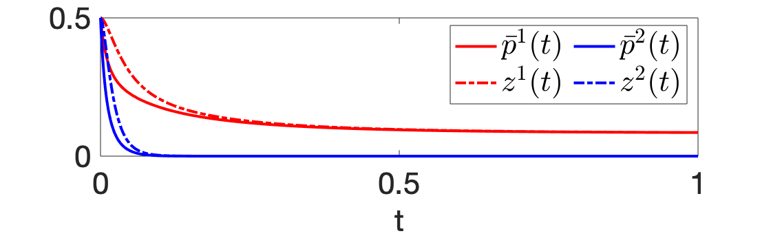
Figure 3: Simulation with two viruses, one (blue) converging to eradication, while the other (red) converges to its single-virus endemic equilibrium.

In the simulation depicted in Figure 3, we chose $\delta_{i}^{1}=4.6$, $\delta_{w}^{1}=4$ and $\delta_{i}^{2}=10$, $\delta_{w}^{2}=10$, for all $i\in[15]$. As a consequence, $s(B_{w}^{2}-D_{w}^{2})=-4.2$, so Theorem 1 applies to virus $2$. Consistent with the result in Theorem 1, virus $2$ becomes eradicated exponentially fast. However, since $s(B_{w}^{1}-D_{w}^{1})=0.3$, virus $1$ fulfills the conditions for Proposition 2, and furthermore, once virus $1$ is eradicated, the system is essentially a single-virus system. Treated as such, virus $1$ satisfies the conditions in Theorem 3. In line with the result in Theorem 3, virus $1$ converges to a single-virus endemic equilibrium. Insofar as it can be determined by varying $y^{1}(0)$ in $\mathcal{D}^{1}$, this single-virus endemic equilibrium appears to be unique and asymptotically stable.

Figure 4: Simulation with two viruses (red and blue), converging to a coexisting equilibrium.

In the simulation depicted in Figure 4, we chose $\delta_{i}^{1}=1.5$ for $i\in[8]$, and $\delta_{i}^{1}=2$ for $i\in[15]\setminus[8]$, with $\delta_{w}^{1}=1$. Relating these choices of parameters for virus $1$ to Figure 2, this corresponds to a low healing rate north of the river Mälaren and a high healing rate south of the river. Mirroring this pattern, we chose $\delta_{i}^{2}=2$ for $i\in[8]$, and $\delta_{i}^{2}=1.5$ for $i\in[15]\setminus[8]$, with $\delta_{w}^{2}=1$. With these parameters, it follows that $s(B_{w}^{1}-D_{w}^{1})=2.8$, and $s(B_{w}^{2}-D_{w}^{2})=2.8$. Hence, both viruses fulfill the conditions for Proposition 2, providing the existence of exactly two single-virus endemic equilibria, namely $(\tilde{y}^{1},\textbf{0})$ and $(\textbf{0},\tilde{y}^{2})$. $\tilde{y}^{1}$ can be approximated by setting $y^{1}(0)>\textbf{0}$ and $y^{2}(0)=\textbf{0}$, and running the simulation for a sufficiently long period of time $T$. Then, assuming that $\tilde{y}^{1}\approx y^{1}(T)$, and, with an analogous approximation for virus $2$, $\tilde{y}^{2}\approx y^{2}(T)$, we obtain $s((I-X(\tilde{y}^{2}))B_{w}^{1}-D_{w}^{1})=0.2$, and $s((I-X(\tilde{y}^{1}))B_{w}^{2}-D_{w}^{2})=0.2$. As a consequence, this pair of viruses fulfills the conditions for Theorem 5. In line with the result in Theorem 5, we see that there exists a coexisting equilibrium. Moreover, our simulations show that the viral infection levels appear to converge to this coexisting equilibrium. Additionally, regardless of how the initial condition is varied within $\mathcal{D}$, barring $y^{1}(0)=\textbf{0}$ or $y^{2}(0)=\textbf{0}$, we observe that all simulations converge to the same coexisting equilibrium. This observation suggests that the coexisting equilibrium might be unique, as well as asymptotically stable.

Figure 5: Simulation with two viruses, with one (blue) converging to eradication, while the other (red) eventually converges to its single-virus endemic equilibrium.

In the simulation depicted in Figure 5, we chose $\delta_{i}^{1}=3$, $\delta_{w}^{1}=3$ and $\delta_{i}^{2}=4$, $\delta_{w}^{2}=4$, for all $i\in[15]$. It follows that $s(B_{w}^{1}-D_{w}^{1})=1.7$, and $s(B_{w}^{2}-D_{w}^{2})=0.9$. Moreover, we have $(D_{w}^{1})^{-1}B_{w}^{1}>(D_{w}^{2})^{-1}B_{w}^{2}$. Therefore, this pair of viruses fulfills the conditions for Theorem 6. In line with the result in Theorem 6, we observe that virus $1$ has a competitive edge, allowing it to persist and converge to its single-virus endemic equilibrium. Meanwhile, virus $2$ is eradicated, despite $s(B_{w}^{2}-D_{w}^{2})$ being positive.

Figure 6: Simulation with two viruses (red and blue), initialized at a coexisting equilibrium. At $t=0.5$ the healing rates of virus $2$ are changed to fulfill Proposition 3.

Figure 7: Simulation with two viruses (red and blue), initialized at a coexisting equilibrium. At $t=0.5$ the healing rates of virus $2$ are changed to fulfill Theorem 8.

The simulations depicted in Figures 6 and 7 were both initialized at the coexisting equilibrium from Figure 4, with all parameters as in that simulation. At $t=0.5$ in the simulation in Figure 6, the healing rates of virus 2, i.e., $\delta_{i}^{2}$, are chosen as in (16), with $\epsilon_{i}^{2}=0$ for all $i\in[15]$. Similarly, at $t=0.5$ in the simulation in Figure 7, the healing rates of virus 2, i.e., $\delta_{i}^{2}$, are chosen as in (17). More specifically, $\delta_{i}^{2}=2$ for $i\in[8]$ as before, but $\delta_{i}^{2}=2.1$ for $i\in[15]\setminus[8]$. We assume that the cost of a strategy $\ell$ (denoted as $\operatorname{cost}^{\ell}$) is given by the sum of all healing rates (i.e., $\operatorname{cost}^{\ell}=\sum_{i=1}^{15}\delta_{i}^{2}$, where $\delta_{i}^{2}$ is chosen as in (16) when $\ell=1$, and as in (17) when $\ell=2$). Our simulations show that $\operatorname{cost}^{1}=61$, whereas $\operatorname{cost}^{2}=33$. However, as seen in Figures 6 and 7, the end result of both strategies is the same. That is, virus 1 persists and reaches its single-virus endemic equilibrium, whereas virus 2 is eradicated. Hence, the strategy in Theorem 8 allows us to eradicate virus 2 at a lower cost than the strategy in Proposition 3, in this case. However, the convergence to the single-virus endemic equilibrium of virus 1 is faster with Proposition 3, as expected from the excessive healing rates.

IX Conclusions

In this paper, we introduced and analyzed a novel SIWS model of competitive, multi-viral spread across a network of population nodes with a shared resource. We established conditions under which a virus is eradicated exponentially fast (resp. asymptotically). We also provided a condition that ensures a virus can reach and sustain a unique, single-virus endemic equilibrium of infection levels across the network. Taken together, these results allowed us to state a necessary and sufficient condition for convergence to the healthy state. Moreover, we presented sufficient conditions under which two viruses can sustain a coexisting equilibrium, that is, where neither virus is eradicated. Conversely, we also provided a necessary condition for the existence of such a coexisting equilibrium. To mitigate the spreading process, we proposed two strategies. The first strategy involved choosing the healing rate of each subpopulation, with respect to each virus, in a suitable manner so as to ensure that all subpopulations converge to the healthy state. The second strategy exploited the notion of competitive exclusion to ensure that in a bi-virus setup, with one virus being malignant and the other benign, the malignant virus becomes eradicated.

The present paper concerns time-invariant SIWS models, whereas in order to obtain a better understanding of real-world scenarios (viz. mobile agents, mutating viruses), it is natural to consider time-varying SIWS models. Secondly, in order to generalize the result on the existence of a coexisting equilibrium (cf. Theorem 5) to more than two viruses, we would need to establish uniqueness of the coexisting equilibrium for the bi-virus case, which is non-trivial.

Appendix

Proof of Theorem 1

Consider a virus $k$ such that $s(B_{w}^{k}-D_{w}^{k})<0$. By Lemma 1 we know that $\mathcal{D}$ is positively invariant with respect to (5), so because $y(0)\in\mathcal{D}$ we have $y(t)\in\mathcal{D}$ for all $t\geq 0$. Then, (4) with respect to virus $k$ can be bounded by:

$$\dot{y}^{k}(t)\leq(B_{w}^{k}-D_{w}^{k})y^{k}(t).$$ (18)

Since $y^{k}(t)\geq\textbf{0}$ for all $t\geq 0$, it follows from Grönwall-Bellman’s Inequality [39, pg 651] that the solution of (4) will be bounded above by the solution of the linear system corresponding to (18) with equality. Since $s(B_{w}^{k}-D_{w}^{k})<0$, we know that 0 is globally exponentially stable in the linear system. Therefore, the eradicated state of virus $k$ is exponentially stable, with domain of attraction containing $\mathcal{D}^{k}$. $\square$

Proof of Lemma 6

Consider an equilibrium $y\in\mathcal{D}$ of system (5). Assume, by way of contradiction, that $\sum_{k=1}^{m}p_{i}^{k}\geq 1$ for some $i\in[n]$. Plugged into (2) under Assumption 1, we obtain

$$\textstyle\sum_{k=1}^{m}\dot{p}_{i}^{k}(t) \leq-\textstyle\sum_{k=1}^{m}\delta_{i}^{k}p_{i}^{k}<0,$$ (19)

where (19) follows from i) Assumption 1, ii) $\sum_{k=1}^{m}p_{i}^{k}\geq 1$ and iii) that $y\in\mathcal{D}$. Note that (19) is a contradiction of the fact that $y$ is an equilibrium, following from the assumption $\sum_{k=1}^{m}p_{i}^{k}\geq 1$ for some $i\in[n]$. Therefore, $\sum_{k=1}^{m}p^{k}\ll\textbf{1}$. Now, assume by way of contradiction that $\sum_{k=1}^{m}z^{k}\geq 1$. Plugged into (2) under Assumption 1, we obtain

$$\textstyle\sum_{k=1}^{m}\dot{z}^{k} <\textstyle\sum_{k=1}^{m}\delta_{w}^{k}\big{(}1-z^{k}\big{)}$$ (20)

$$\leq 0,$$ (21)

where (20) is due to the following reason: First, notice that $\textstyle\sum_{i=1}^{n}c_{i}^{k}=1$ for all $k\in[m]$. Since $\sum_{k=1}^{m}p^{k}\ll\textbf{1}$, it follows that $p_{i}^{k}<1$ for all $i\in[n]$ and $k\in[m]$. Therefore, $\textstyle\sum_{i=1}^{n}c_{i}^{k}p_{i}^{k}<1$. The inequality (21) follows from Assumption 1, and the assumption that $\sum_{k=1}^{m}z^{k}\geq 1$. Note that (21) is a contradiction of the fact that $y$ is an equilibrium of system (5). Since this contradiction follows from the assumption $\sum_{k=1}^{m}z^{k}\geq 1$, we must have $\textstyle\sum_{k=1}^{m}y^{k}\ll\textbf{1}$, and therefore $y^{k}\ll\textbf{1}$, for all $k\in[m]$, for any equilibrium $y\in\mathcal{D}$. Now, for all $k\in[m]$, $y^{k}$ is a equilibrium of (4), so we have

$$(-D_{w}^{k}+(I-\textstyle\sum_{l=1}^{m}X(y^{l}))B_{w}^{k})y^{k} =0,$$

$$\implies(I-\textstyle\sum_{l=1}^{m}X(y^{l}))(D_{w}^{k})^{-1}B_{w}^{k}y^{k} =y^{k}.$$ (22)

Then, since $y^{k}\ll\textbf{1}$, $(I-\textstyle\sum_{l=1}^{m}X(y^{l}))(D_{w}^{k})^{-1}B_{w}^{k}$ is an irreducible nonnegative matrix for all $k\in[m]$. Now, for some $k\in[m]$, assume by way of contradiction that $y^{k}>\textbf{0}$, with $y_{i}^{k}=0$ for all $i\in W$, where $W\subset[n+1]$ is nonempty. Then, by the properties of irreducible nonnegative matrices, $((I-\textstyle\sum_{l=1}^{m}X(y^{l}))(D_{w}^{k})^{-1}B_{w}^{k}y^{k})_{j}>0$ for some $j\in W$. Since $y_{j}^{k}=0$, this contradicts (22), and therefore we must either have $y^{k}\gg\textbf{0}$, or $y^{k}=\textbf{0}$, for each $k\in[m]$. $\square$

Proof of Theorem 2

Consider a virus $k$ such that $s(B_{w}^{k}-D_{w}^{k})\leq 0$. Since $y(0)\in\mathcal{D}$, Lemma 1 states that we have $y(t)\in\mathcal{D}$ for all $t\geq 0$, and further that $\mathcal{D}^{k}$ is positively invariant with respect to (4). Now, note that if $s(B_{w}^{k}-D_{w}^{k})<0$, Theorem 1 implies that the eradicated state is exponentially stable for virus $k$, with domain of attraction containing $\mathcal{D}^{k}$. Hence, the rest of the proof considers the case when $s(B_{w}^{k}-D_{w}^{k})=0$.

Since $(B_{w}^{k}-D_{w}^{k})$ is an irreducible Metzler matrix, by Lemma 2 there exists a positive diagonal matrix $Q^{k}$ such that $\Lambda^{k}\coloneqq((B_{w}^{k}-D_{w}^{k})^{T}Q^{k}+Q^{k}(B_{w}^{k}-D_{w}^{k}))\preccurlyeq 0$. Define the Lyapunov function candidate $V(y^{k}(t))=y^{k}(t)^{T}Q^{k}y^{k}(t)$ with $\mathcal{D}^{k}$ as the domain. Note that $V(y^{k}(t))\succ 0$, and that $V(y^{k}(t))$ fulfills (7). Differentiating $V(y^{k}(t))$ yields

$$\dot{V}(y^{k}(t))=\, 2y^{k}(t)^{T}Q^{k}(B_{w}^{k}-D_{w}^{k})y^{k}(t)$$

$$-2y^{k}(t)^{T}Q^{k}\textstyle\sum_{l=1}^{m}X(y^{l}(t))B_{w}^{k}y^{k}(t)$$

$$\leq\, y^{k}(t)^{T}\Lambda^{k}y^{k}(t)$$

$$-2y^{k}(t)^{T}Q^{k}X(y^{k}(t))B_{w}^{k}y^{k}(t).$$ (23)

We will now show that $\dot{V}(y^{k})<0$ if $y^{k}>\textbf{0}$. First, consider the case where $y_{i}^{k}=0$ for some $i\in[n+1]$. Then, noting that $y^{kT}Q^{k}X(y^{k})B_{w}^{k}y^{k}\geq 0$, we see that (Proof of Theorem 2) is bounded by

$$\dot{V}(y^{k})\leq y^{kT}\Lambda^{k}y^{k}.$$ (24)

Given that $\Lambda^{k}\preccurlyeq 0$, we have $s(\Lambda^{k})\leq 0$. Then, since $\Lambda^{k}$ is an irreducible Metzler matrix, it follows from Lemma 5 that $r\coloneqq s(\Lambda^{k})$ is a simple eigenvalue of $\Lambda^{k}$, with a corresponding eigenvector $\zeta\gg\textbf{0}$. Since we consider the case where $y_{i}^{k}=0$ for some $i\in[n+1]$, $y^{k}$ can not be parallel to $\zeta$. By the Rayleigh-Ritz Theorem [43, Theorem 4.2.2], $y^{kT}\Lambda^{k}y^{k}=ry^{kT}y^{k}$ only if $y^{k}$ is parallel to $\zeta$, and $y^{kT}\Lambda^{k}y^{k}<ry^{kT}y^{k}$ otherwise. Since $r\leq 0$, it follows from (24) that $\dot{V}(y^{k})<0$ when $y_{i}^{k}=0$ for some $i\in[n+1]$. Now, consider the case when $y^{k}\gg\textbf{0}$. Recall that $\Lambda^{k}\preccurlyeq 0$, hence, (Proof of Theorem 2) is bounded by

$$\dot{V}(y^{k})\leq-2y^{kT}Q^{k}X(y^{k})B_{w}^{k}y^{k}.$$ (25)

Since $B_{w}^{k}$ is an irreducible nonnegative matrix, $Q^{k}$ is a positive diagonal matrix and $y^{k}(t)\gg\textbf{0}$, it follows that $y^{kT}Q^{k}X(y^{k})B_{w}^{k}y^{k}>0$. Hence, (25) gives us $\dot{V}(y^{k})<0$ when $y^{k}\gg\textbf{0}$. Then we have $\dot{V}(y^{k})<0$ for all $y^{k}>\textbf{0}$, and it is clear that $\dot{V}(\textbf{0})=0$. Therefore, $\dot{V}(y^{k})\prec 0$. Finally, since $\mathcal{D}^{k}$ is positively invariant with respect to (4), we see that $V(y^{k}(t))$ meets the conditions for Proposition 1. This shows that the eradicated state of virus $k$ is asymptotically stable, with domain of attraction containing $\mathcal{D}^{k}$. $\square$

Proof of Lemma 7

Lemma 1 states that $\mathcal{D}$ is positively invariant with respect to system (5). It remains to be shown that if $y(0)\in\mathcal{D}$, and $y(0)>\textbf{0}$, it follows that $y(t)>\textbf{0}$ for all $t>0$. With $y(0)>\textbf{0}$ we have $y^{k}(0)>\textbf{0}$ for some $k\in[m]$, and by Lemma 1 we know that $y^{k}(t)\geq\textbf{0}$ for all $t>0$. Then, (4) is bounded by

$$\dot{y}^{k}(t)\geq-D_{w}^{k}y^{k}(t),$$ (26)

due to i) $y^{k}(t)\geq\textbf{0}$, and ii) that $(I-\textstyle\sum_{l=1}^{m}X(y^{l}(t)))B_{w}^{k}$ is a nonnegative matrix. Integrating (26) yields

$$y^{k}(t)\geq e^{-tD_{w}^{k}}y^{k}(0)>\textbf{0},$$ (27)

for all $t>0$. The final inequality in (27) follows from the fact that $D_{w}^{k}$ is a positive diagonal matrix. Since $y^{k}(t)>\textbf{0}$, it follows that $y(t)>\textbf{0}$ for all $t>0$. Therefore, $\mathcal{D}\setminus\{\textbf{0}\}$ is positively invariant with respect to system (5). $\square$

Proof of Theorem 3

Part 1 – Proof of existence:

Note that if $y>\textbf{0}$, $\operatorname{diag}(D_{w}^{-1}B_{w}y)$ is a nonnegative diagonal matrix, and therefore the inverse of $(I+\operatorname{diag}(D_{w}^{-1}B_{w}y))$ exists. Define a map $T(y):\mathbb{R}_{+}^{n+1}\rightarrow\mathbb{R}_{+}^{n+1}$ such that

$$T(y)=( I+\operatorname{diag}(D_{w}^{-1}B_{w}y))^{-1}$$

$$\times(D_{w}^{-1}B_{w}y+\operatorname{diag}(D_{w}^{-1}B_{w}y)[\textbf{0}\,y_{n+1}]^{T}).$$

Observe that the components of $T(y)$ are

$$T_{i}(y) =\frac{(D_{w}^{-1}B_{w}y)_{i}}{1+(D_{w}^{-1}B_{w}y)_{i}},\text{ for }i\in[n],$$

$$T_{n+1}(y) =\frac{(D_{w}^{-1}B_{w}y)_{n+1}y_{n+1}+(D_{w}^{-1}B_{w}y)_{n+1}}{1+(D_{w}^{-1}B_{w}y)_{n+1}}.$$

Note that the scalar function $s/(1+s)$ is increasing in $s$, and that $D_{w}^{-1}B_{w}$ is a nonnegative matrix. Therefore, $v\geq z$ implies $T(v)\geq T(z)$. Now, observe that a fixed point of $T(y)$ fulfills

$$y=( I+\operatorname{diag}(D_{w}^{-1}B_{w}y))^{-1}$$

$$\times(D_{w}^{-1}B_{w}y+\operatorname{diag}(D_{w}^{-1}B_{w}y)[\textbf{0}\,y_{n+1}]^{T}).$$ (28)

Multiplying (Proof of Theorem 3) by $(I+\operatorname{diag}(D_{w}^{-1}B_{w}y))$ gives us

$$D_{w}^{-1}B_{w}y+\operatorname{diag}(D_{w}^{-1}B_{w}y)[\textbf{0}\,y_{n+1}]^{T}=(I+\operatorname{diag}(D_{w}^{-1}B_{w}y))y.$$ (29)

Using the identity $\operatorname{diag}(u)v=\operatorname{diag}(v)u$, (29) is equivalent to

$$D_{w}^{-1}B_{w}y+\operatorname{diag}([\textbf{0}\,y_{n+1}]^{T})D_{w}^{-1}B_{w}y=(I+\operatorname{diag}(y)D_{w}^{-1}B_{w})y.$$ (30)

For a given $y\in\mathbb{R}^{n+1}_{+}$, define $X(y)$ to be its diagonalization with the final element $y_{n+1}$ set to zero. As such, subtracting $\operatorname{diag}([\textbf{0}\,y_{n+1}]^{T})D_{w}^{-1}B_{w}y$ from (30) yields

$$D_{w}^{-1}B_{w}y=(I+X(y)D_{w}^{-1}B_{w})y.$$ (31)

Since $X(y)$ and $D_{w}^{-1}$ are diagonal matrices, they commute. Furthermore, by pre-multiplying (31) with $D_{w}$, and suitably rearranging terms, we obtain

$$(B_{w}-D_{w}-X(y)B_{w})y=0.$$ (32)

A solution of equation (32) is clearly an equilibrium of (4) with $m=1$. As such, it suffices to show that $T(y)$ has a non-zero fixed point $\tilde{y}$ in $\mathcal{D}$. We will now show that at least one such fixed point exists. Since $s(B_{w}-D_{w})>0$, by Lemma 3, $\rho(D_{w}^{-1}B_{w})>1$. Note that $D_{w}^{-1}B_{w}$ is an irreducible nonnegative matrix. Hence, by item (i) in Lemma 4, $\lambda^{*}=\rho(D_{w}^{-1}B_{w})$ is a simple eigenvalue of $D_{w}^{-1}B_{w}$. Furthermore, by item (ii) in Lemma 4, we know that the eigenspace of $\lambda^{*}$ is spanned by a vector $y^{*}\gg\textbf{0}$. Then, since $\lambda^{*}>1$, there exists some constant $\epsilon>0$ such that, for all $i\in[n+1]$, we have $\epsilon y_{i}^{*}\leq(\lambda^{*}-1)/\lambda^{*}$, which implies that $1\leq\lambda^{*}/(1+\lambda^{*}\epsilon y_{i}^{*})$. Hence, $\epsilon y_{i}^{*}\leq\lambda^{*}\epsilon y_{i}^{*}/(1+\lambda^{*}\epsilon y_{i}^{*})$, which further implies

$$\epsilon y_{i}^{*}\leq(D_{w}^{-1}B_{w}\epsilon y^{*})_{i}/(1+(D_{w}^{-1}B_{w}\epsilon y^{*})_{i}).$$ (33)

Noting that $(D_{w}^{-1}B_{w}\epsilon y^{*})_{n+1}\epsilon y_{n+1}^{*}>0$, we also have

$$\epsilon y_{n+1}^{*}\leq\frac{(D_{w}^{-1}B_{w}\epsilon y^{*})_{n+1}\epsilon y_{n+1}^{*}+(D_{w}^{-1}B_{w}\epsilon y^{*})_{n+1}}{1+(D_{w}^{-1}B_{w}\epsilon y^{*})_{n+1}}.$$ (34)

Due to the inequalities (33) and (34), we have $T(\epsilon y^{*})\geq\epsilon y^{*}$. Since $y\geq z$ implies $T(y)\geq T(z)$, it follows that for any $y\geq\epsilon y^{*}$ we have $T(y)\geq\epsilon y^{*}$. Consider $T(\textbf{1})$ for $i\in[n]$,

$$T_{i}(\textbf{1})=(D_{w}^{-1}B_{w}\textbf{1})_{i}/(1+(D_{w}^{-1}B_{w}\textbf{1})_{i})\leq 1.$$ (35)

For $i=n+1$, we have

$$T_{n+1}(\textbf{1})=2[c\,\,0]\textbf{1}/(1+[c\,\,0]\textbf{1})\leq 1.$$ (36)

Due to (35) and (36), we have $T(\textbf{1})\leq\textbf{1}$. Since $v\geq w$ implies $T(v)\geq T(w)$, it follows that $T(y)\leq\textbf{1}$ if $y\leq\textbf{1}$. By Brouwer’s fixed-point theorem [44, Theorem 9.3], there is at least one fixed point of $T(y)$ in the domain $\{y:\epsilon y^{*}\leq y\leq\textbf{1}\}$. Since a fixed point of $T(y)$ is equivalent to an equilibrium of (5), by Lemma 6, any fixed point must fulfill $y\ll\textbf{1}$.

In conclusion, the map $T(y)$ has at least one fixed point in the domain $\{y:\epsilon y^{*}\leq y\ll\textbf{1}\}$, and therefore system (5) has at least one equilibrium $\tilde{y}\in\mathcal{D}$ such that $\textbf{0}\ll\tilde{y}\ll\textbf{1}$.

Part 2 – Proof of uniqueness

We will now prove that the single-virus endemic equilibrium is unique. Suppose that there are two single-virus endemic equilibria, $\tilde{y}$ and $\tilde{\mathbf{y}}$. By Lemma 6 we have $\tilde{y}\gg\textbf{0}$ and $\tilde{\mathbf{y}}\gg\textbf{0}$. Let $\kappa=\max_{i\in[n+1]}\tilde{y}_{i}/\tilde{\mathbf{y}}_{i}$. First we show that $\kappa$ is given by

$$\kappa=\max_{i\in[n]}\tilde{y}_{i}/\tilde{\mathbf{y}}_{i}.$$ (37)

To do this, assume by way of contradiction that $\kappa=\tilde{y}_{n+1}/\tilde{\mathbf{y}}_{n+1}$, and $\kappa>\tilde{y}_{i}/\tilde{\mathbf{y}}_{i}$, for all $i\in[n]$. Note that since both $\tilde{y}$ and $\tilde{\mathbf{y}}$ are equilibria of system (4), we have

$$\begin{split}\tilde{y}_{n+1}&=[c\,\,0]\tilde{y}=\textstyle\sum_{i}^{n}c_{i}\tilde{y}_{i},\\ \tilde{\mathbf{y}}_{n+1}&=[c\,\,0]\tilde{\mathbf{y}}=\textstyle\sum_{i}^{n}c_{i}\tilde{\mathbf{y}}_{i}.\end{split}$$ (38)

Since we assume that $\kappa>\tilde{y}_{i}/\tilde{\mathbf{y}}_{i}$, we have $\kappa\tilde{\mathbf{y}}_{i}>\tilde{y}_{i}$, for all $i\in[n]$. Then, (38) gives us

$$\tilde{y}_{n+1}=\textstyle\sum_{i}^{n}c_{i}\tilde{y}_{i}<\textstyle\kappa\sum_{i}^{n}c_{i}\tilde{\mathbf{y}}_{i}=\kappa\tilde{\mathbf{y}}_{n+1},$$

Hence, $\kappa>\tilde{y}_{n+1}/\tilde{\mathbf{y}}_{n+1}$, which contradicts the assumption that $\kappa=\tilde{y}_{n+1}/\tilde{\mathbf{y}}_{n+1}$. Therefore, $\kappa$ must be given by equation (37). Now, by (37) we know that $\tilde{y}\leq\kappa\tilde{\mathbf{y}}$. For some $j\in[n]$ we have $\tilde{y}_{j}=\kappa\tilde{\mathbf{y}}_{j}$. Assume, by way of contradiction, that $\kappa>1$. Then, using the fact that an equilibrium of (4) also constitutes a fixed point of $T(y)$ (see part 1 of this proof), we have

$$\tilde{y}_{j} =(D_{w}^{-1}B_{w}\tilde{y})_{j}/(1+(D_{w}^{-1}B_{w}\tilde{y})_{j})$$

$$\leq(D_{w}^{-1}B_{w}\kappa\tilde{\mathbf{y}})_{j}/(1+(D_{w}^{-1}B_{w}\kappa\tilde{\mathbf{y}})_{j})$$ (39)

$$<\kappa(D_{w}^{-1}B_{w}\tilde{\mathbf{y}})_{j}/(1+(D_{w}^{-1}B_{w}\tilde{\mathbf{y}})_{j})$$ (40)

$$=\kappa\tilde{\mathbf{y}}_{j}$$ (41)

$$=\tilde{y}_{j},$$ (42)

where (39) follows from $\tilde{y}\leq\kappa\tilde{\mathbf{y}}$ and that $T(v)\geq T(w)$ whenever $v\geq w$, (40) follows from the assumption $\kappa>1$, and (41) follows from the fact that $\tilde{\mathbf{y}}$ is an equilibrium of (4). Note that (42) is a contradiction, following from our assumption that $\kappa>1$. Hence, $\kappa\leq 1$, meaning that $\tilde{y}\leq\tilde{\mathbf{y}}$. Switching the roles of $\tilde{y}$ and $\tilde{\mathbf{y}}$, we see that $\tilde{\mathbf{y}}\leq\tilde{y}$. Therefore, $\tilde{y}=\tilde{\mathbf{y}}$, and thus the equilibrium is unique.

Part 3 – Proof of asymptotic stability
Recall that $\tilde{y}$ is the unique single-virus endemic equilibrium of system (4) in $\mathcal{D}$, where $\textbf{0}\ll\tilde{y}\ll\textbf{1}$, and

$$(-D_{w}+(I-X(\tilde{y}))B_{w})\tilde{y}=\textbf{0}.$$ (43)

For $y(t)\in\mathcal{D}$, let $\Delta y(t)=y(t)-\tilde{y}$. From (4) it follows that

$$\Delta\dot{y}(t) =(-D_{w}+(I-X(\Delta y)-X(\tilde{y}))B_{w})(\Delta y+\tilde{y})$$

$$=(-D_{w}+(I-X(\tilde{y}))B_{w})\Delta y-X(\Delta y)B_{w}y$$ (44)

$$=(-D_{w}+(I-X(\tilde{y}))B_{w}-X(B_{w}y))\Delta y,$$ (45)

where (44) follows from (43), and (45) follows from $X(u)v=X(v)u$. Now, since $D_{w}$ is invertible, (43) is equivalent to

$$(I-X(\tilde{y}))D_{w}^{-1}B_{w}\tilde{y}=\tilde{y}.$$ (46)

Since $B_{w}$ is an irreducible nonnegative matrix, and $D_{w}$ is a positive diagonal matrix, $\tilde{y}\ll\textbf{1}$ ensures that $(I-X(\tilde{y}))D_{w}^{-1}B_{w}$ is an irreducible nonnegative matrix, and in turn that $(-D_{w}+(I-X(\tilde{y}))B_{w})$ is an irreducible Metzler matrix. Therefore, since $\tilde{y}\gg\textbf{0}$, item (iii) in Lemma 4 applied to (46) gives us $\rho((I-X(\tilde{y}))D_{w}^{-1}B_{w})=1$, which by Lemma 3 is equivalent to $s(-D_{w}+(I-X(\tilde{y}))B_{w})=0$. Then, Lemma 2 guarantees the existence of a positive diagonal matrix $Q$ such that $\Psi\coloneqq(-D_{w}+(I-X(\tilde{y}))B_{w})^{T}Q+Q(-D_{w}+(I-X(\tilde{y}))B_{w})\preccurlyeq 0$. Define the Lyapunov function candidate $V(\Delta y(t))=\Delta y(t)^{T}Q\Delta y(t)$, with $y(t)\in\mathcal{D}\setminus\{\textbf{0}\}$ as the domain. Note that $V(\Delta y(t))\succ 0$ and that $V(\Delta y(t))$ fulfills (7). Differentiating $V(\Delta y(t))$ with respect to $t$ yields

$$\dot{V}(\Delta y(t)) =2\Delta y^{T}Q(-D_{w}+(I-X(\tilde{y}))B_{w})\Delta y$$

$$\,\,\,\,\,-2\Delta y^{T}QX(B_{w}y)\Delta y$$ (47)

$$=\Delta y^{T}\Psi\Delta y-2\Delta y^{T}QX(B_{w}y)\Delta y$$ (48)

where (47) makes use of (45). We want to show that $\dot{V}(\Delta y(t))<0$ for all $y(t)\in\mathcal{D}\setminus\{\textbf{0}\}$ such that $\Delta y(t)=y(t)-\tilde{y}\neq\textbf{0}$. First, consider all $y(t)\in\mathcal{D}\setminus\{\textbf{0}\}$ such that $y(t)\gg\textbf{0}$. Combining (48) and the fact that $\Psi\preccurlyeq 0$ gives us

$$\dot{V}(\Delta y(t)) \leq-2\Delta y(t)^{T}QX(B_{w}y(t))\Delta y(t).$$ (49)

Note that, given $y(t)\gg\textbf{0}$, $QX(B_{w}y(t))$ is a positive diagonal matrix, and thus $QX(B_{w}y(t))\succ 0$. Therefore, (49) gives us $\dot{V}(\Delta y(t))<0$ for all $y(t)\in\mathcal{D}\setminus\{\textbf{0}\}$ such that $y(t)\gg\textbf{0}$, $\Delta y(t)=y(t)-\tilde{y}\neq\textbf{0}$. Now, consider all $y(t)\in\mathcal{D}\setminus\{\textbf{0}\}$ such that $y(t)>\textbf{0}$, $y_{i}(t)=0$ for some $i\in[n+1]$. Note that, given $y(t)>\textbf{0}$, $QX(B_{w}y(t))$ is a nonnegative diagonal matrix. Then (48) can be bounded by

$$\dot{V}(\Delta y(t)) \leq\Delta y(t)^{T}\Psi\Delta y(t).$$ (50)

Given that $(-D_{w}+(I-X(\tilde{y}))B_{w})$ is an irreducible Metzler matrix and $Q$ is a positive diagonal matrix, $\Psi$ is an irreducible Metzler matrix. Employing (43), we see that

$$\tilde{y}^{T}\Psi\tilde{y}=0.$$ (51)

Item (i) in Lemma 5 stipulates that $r\coloneqq s(\Psi)$ is a simple eigenvalue of $\Psi$. Due to $\Psi\preccurlyeq 0$ and the Rayleigh-Ritz Theorem [43, Theorem 4.2.2], it follows from (51) that $r=0$, and that $\tilde{y}$ spans the eigenspace of $r$. As such, due to $\tilde{y}\gg\textbf{0}$, and $y(t)>\textbf{0}$ with $y_{i}(t)=0$ for some $i\in[n+1]$, $y(t)$ can not be parallel to $\tilde{y}$. As a consequence, $\Delta y(t)$ can not be parallel to $\tilde{y}$. By the Rayleigh-Ritz Theorem [43, Theorem 4.2.2], $x^{T}\Psi x=rx^{T}x$ only if $x$ is parallel to $\tilde{y}$, and $x^{T}\Psi x<rx^{T}x$ otherwise. Therefore, $r=0$ together with (50) gives us $\dot{V}(\Delta y(t))<0$ for all $y(t)\in\mathcal{D}\setminus\{\textbf{0}\}$ such that $y(t)\gg\textbf{0}$ and $y(t)-\tilde{y}\neq\textbf{0}$.

Thus, we have $\dot{V}(\Delta y(t))<0$ for all $y(t)\in\mathcal{D}\setminus\{\textbf{0}\}$ such that $\Delta y(t)=y(t)-\tilde{y}\neq\textbf{0}$, and it is clear that $\dot{V}(\textbf{0})=0$. Therefore, $\dot{V}(\Delta y(t))\prec 0$ for $y(t)\in\mathcal{D}\setminus\{\textbf{0}\}$.

Finally, from Lemma 7 we have that $\mathcal{D}\setminus\{\textbf{0}\}$ is a positively invariant set with respect to (5). Thus, we see that $V(\Delta y(t))$ meets the conditions for Proposition 1 with respect to the shifted coordinates $\Delta y(t)=y(t)-\tilde{y}$, for all $y(t)\in\mathcal{D}\setminus\{\textbf{0}\}$. This shows that the unique single-virus endemic equilibrium $\tilde{y}$ is asymptotically stable, with domain of attraction containing $\mathcal{D}\setminus\{\textbf{0}\}$. Thus, with parts 1, 2 and 3 in place, the proof of Theorem 3 is concluded. $\square$

Proof of Proposition 2

Suppose that, for some $k\in[m]$, $B_{w}^{k}$ is irreducible and $s(B_{w}^{k}-D_{w}^{k})>0$, and that $y^{l}=\textbf{0}$ for all $l\in[m]$, $l\neq k$. Then the dynamics of virus $k$ can be written as

$$\dot{y}^{k}(t)=\big{(}-D_{w}^{k}+(I-X(y^{k}(t)))B_{w}^{k}\big{)}y^{k}(t).$$ (52)

Note that (52) corresponds to the dynamics of the single-virus case. Therefore, since $B_{w}^{k}$ is irreducible and $s(B_{w}^{k}-D_{w}^{k})>0$, it follows from the first and second parts of the proof of Theorem 3 that there exists a unique single-virus endemic equilibrium of the form $(\textbf{0},\dots,\tilde{y}^{k},\dots,\textbf{0})$, with $\textbf{0}\ll\tilde{y}^{k}\ll\textbf{1}$ in $\mathcal{D}$. This holds for each $k\in[m]$ such that $B_{w}^{k}$ is irreducible and $s(B_{w}^{k}-D_{w}^{k})>0$, by repeating the arguments above. $\square$

Proof of Theorem 5

Recall that for $k\in[2]$, Assumption 1 implies that $D_{w}^{k}$ is a positive diagonal matrix, and therefore invertible. Furthermore, note that $(I+\operatorname{diag}((D_{w}^{1})^{-1}B_{w}^{1}y^{1}))$ and $(I+\operatorname{diag}((D_{w}^{2})^{-1}B_{w}^{2}y^{2}))$ are positive diagonal matrices whenever $y^{1}\geq 0$ and $y^{2}\geq 0$, and are then also invertible. For $y\in\mathbb{R}^{n+1}_{+}$, define $X(y)$ to be $\operatorname{diag}(y)$ with $y_{n+1}$ set to zero. Define the maps $T^{1}(y^{1},y^{2}):[0,1]^{n+1}\times[0,1]^{n+1}\rightarrow[0,1]^{n+1}$, and $T^{2}(y^{1},y^{2}):[0,1]^{n+1}\times[0,1]^{n+1}\rightarrow[0,1]^{n+1}$, such that

$$T^{1}(y^{1},y^{2})=(I+\operatorname{diag}((D_{w}^{1})^{-1}B_{w}^{1}y^{1}))^{-1}$$

$$\times((I-X(y^{2}))(D_{w}^{1})^{-1}B_{w}^{1}y^{1}+\operatorname{diag}((D_{w}^{1})^{-1}B_{w}^{1}y^{1})[\textbf{0}\,y_{n+1}^{1}]^{T}),$$

$$T^{2}(y^{1},y^{2})=(I+\operatorname{diag}((D_{w}^{2})^{-1}B_{w}^{2}y^{2}))^{-1}$$

$$\times((I-X(y^{1}))(D_{w}^{2})^{-1}B_{w}^{2}y^{2}+\operatorname{diag}((D_{w}^{2})^{-1}B_{w}^{2}y^{2})[\textbf{0}\,y_{n+1}^{2}]^{T}).$$

For $i\in[n]$, the $i^{\text{th}}$ components of the maps are

$$T_{i}^{1}(y^{1},y^{2}) =\frac{(1-y_{i}^{2})((D_{w}^{1})^{-1}B_{w}^{1}y^{1})_{i}}{1+((D_{w}^{1})^{-1}B_{w}^{1}y^{1})_{i}},$$

$$T_{i}^{2}(y^{1},y^{2}) =\frac{(1-y_{i}^{1})((D_{w}^{2})^{-1}B_{w}^{2}y^{2})_{i}}{1+((D_{w}^{2})^{-1}B_{w}^{2}y^{2})_{i}}.$$

Furthermore, the $(n+1)^{\text{th}}$ components of the maps are

$$T_{n+1}^{1}(y^{1},y^{2}) =\frac{((D_{w}^{1})^{-1}B_{w}^{1}y^{1})_{n+1}+(D_{w}^{1})^{-1}B_{w}^{1}y^{1})_{n+1}y_{n+1}^{1}}{1+((D_{w}^{1})^{-1}B_{w}^{1}y^{1})_{n+1}},$$

$$T_{n+1}^{2}(y^{1},y^{2}) =\frac{((D_{w}^{2})^{-1}B_{w}^{2}y^{2})_{n+1}+((D_{w}^{2})^{-1}B_{w}^{2}y^{2})_{n+1}y_{n+1}^{2}}{1+((D_{w}^{2})^{-1}B_{w}^{2}y^{2})_{n+1}}.$$

Note that the scalar function $s/(1+s)$ is increasing in $s$, and for $k\in[2]$, the matrix $(D_{w}^{k})^{-1}B_{w}^{k}$ is nonnegative, therefore, $T_{i}^{k}$ is an increasing function in $y_{j}^{k}$ for all $i,j\in[n+1]$. Moreover, $T_{i}^{1}$ is a decreasing function in $y_{i}^{2}$ and $T_{i}^{2}$ is a decreasing function in $y_{i}^{1}$, for all $i\in[n]$. Hence, for any $y^{1},y^{2}\in[0,1]^{n+1}$, if $v\geq z$ it follows that

$$\begin{split}T^{1}(v,y^{2})\geq T^{1}(z,y^{2})&,\,\,T^{1}(y^{1},v)\leq T^{1}(y^{1},z),\\ T^{2}(v,y^{2})\leq T^{2}(z,y^{2})&,\,\,T^{2}(y^{1},v)\geq T^{2}(y^{1},z).\end{split}$$ (53)

The inequalities in (53) state that $T^{k}(y^{1},y^{2})$ is increasing in its $k^{\rm{th}}$ argument and decreasing in its other argument, for $k\in[2]$. Let $y=(y^{1},y^{2})$, and let $T(y):[0,1]^{2(n+1)}\rightarrow[0,1]^{2(n+1)}$ be the map $T(y)=(T^{1}(y),T^{2}(y))$. A fixed point of $T(y)$ fulfills

$$y^{1}=(I+\operatorname{diag}((D_{w}^{1})^{-1}B_{w}^{1}y^{1}))^{-1}$$

$$\times((I-X(y^{2}))(D_{w}^{1})^{-1}B_{w}^{1}y^{1}+\operatorname{diag}((D_{w}^{1})^{-1}B_{w}^{1}y^{1})[\textbf{0}\,y_{n+1}^{1}]^{T}),$$

$$y^{2}=(I+\operatorname{diag}((D_{w}^{2})^{-1}B_{w}^{2}y^{2}))^{-1}$$

$$\times((I-X(y^{1}))(D_{w}^{2})^{-1}B_{w}^{2}y^{2}+\operatorname{diag}((D_{w}^{2})^{-1}B_{w}^{2}y^{2})[\textbf{0}\,y_{n+1}^{2}]^{T}).$$ (54)

Pre-multiplying the first line (resp. second line) of (Proof of Theorem 5) by $(I+\operatorname{diag}((D_{w}^{1})^{-1}B_{w}^{1}y^{1}))$ (resp. $(I+\operatorname{diag}((D_{w}^{2})^{-1}B_{w}^{2}y^{2}))$) gives us

$$(I+\operatorname{diag}((D_{w}^{1})^{-1}B_{w}^{1}y^{1}))y^{1}=$$

$$(I-X(y^{2}))(D_{w}^{1})^{-1}B_{w}^{1}y^{1}+\operatorname{diag}((D_{w}^{1})^{-1}B_{w}^{1}y^{1})[\textbf{0}\,y_{n+1}^{1}]^{T},$$

$$(I+\operatorname{diag}((D_{w}^{2})^{-1}B_{w}^{2}y^{2}))y^{2}=$$ (55)

$$(I-X(y^{1}))(D_{w}^{2})^{-1}B_{w}^{2}y^{2}+\operatorname{diag}((D_{w}^{2})^{-1}B_{w}^{2}y^{2})[\textbf{0}\,y_{n+1}^{2}]^{T}.$$

Rearranging (55), making use of the identity $\operatorname{diag}(u)v=\operatorname{diag}(v)u$, and subtracting $\operatorname{diag}([\textbf{0}\,y_{n+1}^{1}]^{T})(D_{w}^{1})^{-1}B_{w}^{1}y^{1}$ (resp. $\operatorname{diag}([\textbf{0}\,y_{n+1}^{2}]^{T})(D_{w}^{2})^{-1}B_{w}^{2}y^{2}$) from the first (resp. second line) yields

$$\begin{split}(I-X(y^{1})-X(y^{2}))(D_{w}^{1})^{-1}B_{w}^{1}y^{1}&=y^{1},\\ (I-X(y^{1})-X(y^{2}))(D_{w}^{2})^{-1}B_{w}^{2}y^{2}&=y^{2}.\end{split}$$ (56)

Making use of the fact that diagonal matrices commute, pre-multiplying the first line (resp. second line) of (56) by $D_{w}^{1}$ (resp. $D_{w}^{2}$), and rearranging terms gives us

$$\begin{split}(-D_{w}^{1}+(I-X(y^{1})-X(y^{2}))B_{w}^{1})y^{1}&=\textbf{0},\\ (-D_{w}^{2}+(I-X(y^{1})-X(y^{2}))B_{w}^{2})y^{2}&=\textbf{0}.\end{split}$$ (57)

Comparing (57) with (4), it follows that a fixed point of $T(y)$ constitutes an equilibrium of system (5) and vice versa. It suffices to show that $T(y)$ has a fixed point $\hat{y}=(\hat{y}^{1},\hat{y}^{2})\gg\textbf{0}$, such that $\hat{y}^{1}+\hat{y}^{2}\leq\textbf{1}$.

Recall that $(\tilde{y}^{1},\textbf{0})$ and $(\textbf{0},\tilde{y}^{2})$ are single-virus endemic equilibria of system (5). Consider $T^{1}(\tilde{y}^{1},y^{2})$. By assumption, $(\tilde{y}^{1},\textbf{0})$ is an equilibrium of (5), therefore $T^{1}(\tilde{y}^{1},\textbf{0})=\tilde{y}^{1}$. By the inequalities in (53) we have $T^{1}(\tilde{y}^{1},y^{2})\leq\tilde{y}^{1}$, and thus $T^{1}(y^{1},y^{2})\leq\tilde{y}^{1}$, for all $y^{1}\leq\tilde{y}^{1}$. Analogously, it can be shown that we have $T^{2}(y^{1},y^{2})\leq\tilde{y}^{2}$, for all $y^{2}\leq\tilde{y}^{2}$. Thus,

$$T(y^{1},y^{2})\leq(\tilde{y}^{1},\tilde{y}^{2}),$$ (58)

whenever $(y^{1},y^{2})\leq(\tilde{y}^{1},\tilde{y}^{2})$. Now, by assumption, $s(-D_{w}^{1}+(I-X(\tilde{y}^{2}))B_{w}^{1})>0$, and, since $D_{w}^{1}$ and $(I-X(\tilde{y}^{2}))$ are positive diagonal matrices and $B_{w}^{1}$ is an irreducible nonnegative matrix, $(-D_{w}^{1}+(I-X(\tilde{y}^{2}))B_{w}^{1})$ is an irreducible Metzler matrix. Then, by Lemma 3 and the fact that diagonal matrices commute, we have $\rho((I-X(\tilde{y}^{2}))(D_{w}^{1})^{-1}B_{w}^{1})>1$. Further, since $((I-X(\tilde{y}^{2}))(D_{w}^{1})^{-1}B_{w}^{1})$ is an irreducible nonnegative matrix, by item (i) in Lemma 4 we know that $\lambda^{1}=\rho((I-X(\tilde{y}^{2}))(D_{w}^{1})^{-1}B_{w}^{1})$ is a simple eigenvalue of this matrix. Furthermore, by item (ii) in Lemma 4, we know that the eigenspace of $\lambda^{1}$ is spanned by a vector $\bar{\bar{y}}^{1}\gg\textbf{0}$. Analogously we get $\lambda^{2}=\rho((I-X(\tilde{y}^{1}))(D_{w}^{2})^{-1}B_{w}^{2})>1$, and the corresponding eigenvector $\bar{\bar{y}}^{2}\gg\textbf{0}$.

With the eigenvectors $\bar{\bar{y}}^{1},\bar{\bar{y}}^{2}$ in place, we see that since $(D_{w}^{1})^{-1}B_{w}^{1}$ and $(D_{w}^{2})^{-1}B_{w}^{2}$ are irreducible nonnegative matrices, we have $((D_{w}^{1})^{-1}B_{w}^{1}\bar{\bar{y}}^{1})_{i}>0$, and $((D_{w}^{2})^{-1}B_{w}^{2}\bar{\bar{y}}^{2})_{i}>0$, for all $i\in[n+1]$. Further, given that $\bar{\bar{y}}^{1}\gg\textbf{0},\bar{\bar{y}}^{2}\gg\textbf{0},\tilde{y}^{1}\gg\textbf{0}$, and $\tilde{y}^{2}\gg\textbf{0}$, we have $\tilde{y}_{i}^{1}/\bar{\bar{y}}_{i}^{1}>0$, and $\tilde{y}_{i}^{2}/\bar{\bar{y}}_{i}^{2}>0$, for all $i\in[n+1]$. Moreover, note that $\lambda^{1}-1>0$ and $\lambda^{2}-1>0$. Hence, there exist $\epsilon^{1}>0$ and $\epsilon^{2}>0$ such that

$$\begin{split}\epsilon^{1}&<\min\left\{\frac{\lambda^{1}-1}{\max_{i\in[n+1]}((D_{w}^{1})^{-1}B_{w}^{1}\bar{\bar{y}}^{1})_{i}},\,\min_{i\in[n+1]}\frac{\tilde{y}_{i}^{1}}{\bar{\bar{y}}_{i}^{1}}\right\},\\ \epsilon^{2}&<\min\left\{\frac{\lambda^{2}-1}{\max_{i\in[n+1]}((D_{w}^{2})^{-1}B_{w}^{2}\bar{\bar{y}}^{2})_{i}},\,\min_{i\in[n+1]}\frac{\tilde{y}_{i}^{2}}{\bar{\bar{y}}_{i}^{2}}\right\}.\end{split}$$ (59)

From (59) follows that

$$\begin{split}1+\textstyle\max_{i\in[n]}((D_{w}^{1})^{-1}B_{w}^{1}\epsilon^{1}\bar{\bar{y}}^{1})_{i}&<\lambda^{1},\\ 1+\textstyle\max_{i\in[n]}((D_{w}^{2})^{-1}B_{w}^{2}\epsilon^{2}\bar{\bar{y}}^{2})_{i}&<\lambda^{2}.\end{split}$$ (60)

Employing (60) it follows that, for all $i\in[n]$, we have

$$T_{i}^{1}(\epsilon^{1}\bar{\bar{y}}^{1},\tilde{y}^{2}) =\frac{((I-X(\tilde{y}^{2}))(D_{w}^{1})^{-1}B_{w}^{1}\epsilon^{1}\bar{\bar{y}}^{1})_{i}}{1+((D_{w}^{1})^{-1}B_{w}^{1}\epsilon^{1}\bar{\bar{y}}^{1})_{i}}$$

$$=\frac{\lambda^{1}\epsilon^{1}\bar{\bar{y}}_{i}^{1}}{1+((D_{w}^{1})^{-1}B_{w}^{1}\epsilon^{1}\bar{\bar{y}}^{1})_{i}}>\epsilon^{1}\bar{\bar{y}}_{i}^{1},$$

$$T_{i}^{2}(\tilde{y}^{1},\epsilon^{2}\bar{\bar{y}}^{2}) =\frac{((I-X(\tilde{y}^{1}))(D_{w}^{2})^{-1}B_{w}^{2}\epsilon^{2}\bar{\bar{y}}^{2})_{i}}{1+((D_{w}^{2})^{-1}B_{w}^{2}\epsilon^{2}\bar{\bar{y}}^{2})_{i}}$$

$$=\frac{\lambda^{2}\epsilon^{2}\bar{\bar{y}}_{i}^{2}}{1+((D_{w}^{2})^{-1}B_{w}^{2}\epsilon^{2}\bar{\bar{y}}^{2})_{i}}>\epsilon^{2}\bar{\bar{y}}_{i}^{2}.$$

For $T_{n+1}^{1}$ and $T_{n+1}^{2}$, note that $((D_{w}^{1})^{-1}B_{w}^{1}\epsilon^{1}\bar{\bar{y}}^{1})_{n+1}\bar{\bar{y}}_{n+1}^{1}>0$ and $((D_{w}^{2})^{-1}B_{w}^{2}\epsilon^{2}\bar{\bar{y}}^{2})_{n+1}\bar{\bar{y}}_{n+1}^{2}>0$, respectively. Therefore

$$T_{n+1}^{1}(\epsilon^{1}\bar{\bar{y}}^{1},\tilde{y}^{2})$$

$$=\frac{((I-X(\tilde{y}^{2}))(D_{w}^{1})^{-1}B_{w}^{1}\epsilon^{1}\bar{\bar{y}}^{1})_{n+1}}{1+((D_{w}^{1})^{-1}B_{w}^{1}\epsilon^{1}\bar{\bar{y}}^{1})_{n+1}}+\frac{((D_{w}^{1})^{-1}B_{w}^{1}\epsilon^{1}\bar{\bar{y}}^{1})_{n+1}\bar{\bar{y}}_{n+1}^{1}}{1+((D_{w}^{1})^{-1}B_{w}^{1}\epsilon^{1}\bar{\bar{y}}^{1})_{n+1}}$$

$$\geq\frac{\lambda^{1}\epsilon^{1}\bar{\bar{y}}_{n+1}^{1}}{1+((D_{w}^{1})^{-1}B_{w}^{1}\epsilon^{1}\bar{\bar{y}}^{1})_{n+1}}>\epsilon^{1}\bar{\bar{y}}_{n+1}^{1},$$

$$T_{n+1}^{2}(\tilde{y}^{1},\epsilon^{2}\bar{\bar{y}}^{2})$$

$$=\frac{((I-X(\tilde{y}^{1}))(D_{w}^{2})^{-1}B_{w}^{2}\epsilon^{2}\bar{\bar{y}}^{2})_{n+1}}{1+((D_{w}^{2})^{-1}B_{w}^{2}\epsilon^{2}\bar{\bar{y}}^{2})_{n+1}}+\frac{((D_{w}^{2})^{-1}B_{w}^{2}\epsilon^{2}\bar{\bar{y}}^{2})_{n+1}\bar{\bar{y}}_{n+1}^{2}}{1+((D_{w}^{2})^{-1}B_{w}^{2}\epsilon^{2}\bar{\bar{y}}^{2})_{n+1}}$$

$$\geq\frac{\lambda^{2}\epsilon^{2}\bar{\bar{y}}_{n+1}^{2}}{1+((D_{w}^{2})^{-1}B_{w}^{2}\epsilon^{2}\bar{\bar{y}}^{2})_{n+1}}>\epsilon^{2}\bar{\bar{y}}_{n+1}^{2}.$$

Given that (59) implies $\epsilon^{1}\bar{\bar{y}}^{1}<\tilde{y}^{1}$ and $\epsilon^{2}\bar{\bar{y}}^{2}<\tilde{y}^{2}$, by the inequalities in (53) we have $T^{1}(\epsilon^{1}\bar{\bar{y}}^{1},y^{2})>\epsilon^{1}\bar{\bar{y}}^{1}$ whenever $\epsilon^{2}\bar{\bar{y}}^{2}\leq y^{2}\leq\tilde{y}^{2}$, and $T^{2}(y^{1},\epsilon^{2}\bar{\bar{y}}^{2})>\epsilon^{2}\bar{\bar{y}}^{2}$ whenever $\epsilon^{1}\bar{\bar{y}}^{1}\leq y^{1}\leq\tilde{y}^{1}$. Further application of the inequalities in (53) yields

$$T^{1}(y^{1},y^{2})>\epsilon^{1}\bar{\bar{y}}^{1},\,\,\,T^{2}(y^{1},y^{2})>\epsilon^{2}\bar{\bar{y}}^{2},$$ (61)

whenever $(\epsilon^{1}\bar{\bar{y}}^{1},\epsilon^{2}\bar{\bar{y}}^{2})\leq(y^{1},y^{2})\leq(\tilde{y}^{1},\tilde{y}^{2})$. Then, (58) and (61) show that $(\epsilon^{1}\bar{\bar{y}}^{1},\epsilon^{2}\bar{\bar{y}}^{2})\leq T(y^{1},y^{2})\leq(\tilde{y}^{1},\tilde{y}^{2})$ whenever $(\epsilon^{1}\bar{\bar{y}}^{1},\epsilon^{2}\bar{\bar{y}}^{2})\leq(y^{1},y^{2})\leq(\tilde{y}^{1},\tilde{y}^{2})$. By Brouwer’s fixed point theorem [44, Theorem 9.3], there exists at least one fixed point of $T(y)$ in the domain $\{y=(y^{1},y^{2}):(\epsilon^{1}\bar{\bar{y}}^{1},\epsilon^{2}\bar{\bar{y}}^{2})\leq(y^{1},y^{2})\leq(\tilde{y}^{1},\tilde{y}^{2})\}$. Recall that a fixed point of $T(y)$ is equivalent to an equilibrium of (5), hence, by Lemma 6, any fixed point of $T(y)$ must fulfill $y^{1}+y^{2}\leq\textbf{1}$. In conclusion, system (5) has at least one coexisting equilibrium $(\hat{y}^{1},\hat{y}^{2})\gg\textbf{0}$ in $\mathcal{D}$, such that $\hat{y}^{1}+\hat{y}^{2}\leq\textbf{1}$. $\square$

Proof of Theorem 6

In order to prove Theorem 6, we require the following lemma.

Lemma 8.

Consider system (5) under Assumption 1 with $m=2$. Suppose that $B_{w}^{1}$ and $B_{w}^{2}$ are irreducible matrices, that $s(B_{w}^{1}-D_{w}^{1})>0$ and $s(B_{w}^{2}-D_{w}^{2})>0$, and that $(D_{w}^{1})^{-1}B_{w}^{1}>(D_{w}^{2})^{-1}B_{w}^{2}$. If $(\tilde{y}^{1},\textbf{0})$ and $(\textbf{0},\tilde{y}^{2})$ are single-virus endemic equilibria of (5), then $\tilde{y}^{1}>\tilde{y}^{2}$. $\blacksquare$

Proof: Given that $\tilde{y}^{1}$ and $\tilde{y}^{2}$ are equilibria of (4), and observing that diagonal matrices commute, we obtain

$$\begin{split}(I-X(\tilde{y}^{1}))(D_{w}^{1})^{-1}B_{w}^{1}\tilde{y}^{1}&=\tilde{y}^{1},\\ (I-X(\tilde{y}^{2}))(D_{w}^{2})^{-1}B_{w}^{2}\tilde{y}^{2}&=\tilde{y}^{2}.\end{split}$$ (62)

By Lemma 6 we have $\textbf{0}\ll\tilde{y}^{1}\ll\textbf{1}$ and $\textbf{0}\ll\tilde{y}^{2}\ll\textbf{1}$. Let $\kappa=\max_{i\in[n+1]}\tilde{y}_{i}^{2}/\tilde{y}_{i}^{1}$, and thus $\tilde{y}^{2}\leq\kappa\tilde{y}^{1}$. Since $(D_{w}^{1})^{-1}B_{w}^{1}>(D_{w}^{2})^{-1}B_{w}^{2}$, and $\textstyle\sum_{i=1}^{n}c_{i}^{k}=1$ for all $k\in[2]$, we have $c^{1}=c^{2}$. Then, by analogous arguments to those in part 2 of the proof of Theorem 3, we know that $\kappa=\max_{i\in[n]}\tilde{y}_{i}^{2}/\tilde{y}_{i}^{1}$. Let $j$ be the index in $[n]$ such that $\tilde{y}_{j}^{2}=\kappa\tilde{y}_{j}^{1}$. Assume, by way of contradiction, that $\kappa>1$, implying $\tilde{y}_{j}^{2}>\tilde{y}_{j}^{1}$. Note that since $(D_{w}^{1})^{-1}B_{w}^{1}>(D_{w}^{2})^{-1}B_{w}^{2}$, with both matrices being irreducible and nonnegative, it follows that $(D_{w}^{1})^{-1}B_{w}^{1}y>(D_{w}^{2})^{-1}B_{w}^{2}y$ for any $y\gg\textbf{0}$. Further, note that $\tilde{y}^{1}\ll\textbf{1}$, ensuring $(1-\tilde{y}_{j}^{1})>0$. Then, (62) gives us

$$\tilde{y}_{j}^{2} =(1-\tilde{y}_{j}^{2})((D_{w}^{2})^{-1}B_{w}^{2}\tilde{y}^{2})_{j}$$

$$\leq(1-\tilde{y}_{j}^{2})((D_{w}^{1})^{-1}B_{w}^{1}\tilde{y}^{2})_{j}$$ (63)

$$<(1-\tilde{y}_{j}^{2})((D_{w}^{1})^{-1}B_{w}^{1}\kappa\tilde{y}^{1})_{j}$$ (64)

$$={(1-\tilde{y}_{j}^{2})}{(1-\tilde{y}_{j}^{1})}^{-1}\kappa\tilde{y}_{j}^{1}$$ (65)

$$={(1-\tilde{y}_{j}^{2})}{(1-\tilde{y}_{j}^{1})}^{-1}\tilde{y}_{j}^{2}$$ (66)

$$<\tilde{y}_{j}^{2},$$ (67)

where (63) follows from $(D_{w}^{1})^{-1}B_{w}^{1}>(D_{w}^{2})^{-1}B_{w}^{2}$, (64) follows from $\tilde{y}^{2}<\kappa\tilde{y}^{1}$, (65) follows from (62), (66) follows from $\tilde{y}_{j}^{2}=\kappa\tilde{y}_{j}^{1}$, and (67) follows from $\tilde{y}_{j}^{2}>\tilde{y}_{j}^{1}$. Note that (67) is a contradiction, following from our assumption that $\kappa>1$. Therefore, $\kappa\leq 1$, and hence, $\tilde{y}^{1}\geq\tilde{y}^{2}$. Assume, by way of contradiction, that $\tilde{y}^{1}=\tilde{y}^{2}=\tilde{y}$. Then $(I-X(\tilde{y}))(D_{w}^{1})^{-1}B_{w}^{1}>(I-X(\tilde{y}))(D_{w}^{2})^{-1}B_{w}^{2}$, and it follows from (62) that

$$\tilde{y} =(I-X(\tilde{y}))(D_{w}^{1})^{-1}B_{w}^{1}\tilde{y}$$

$$>(I-X(\tilde{y}))(D_{w}^{2})^{-1}B_{w}^{2}\tilde{y}=\tilde{y}.$$ (68)

It is clear that (68) is a contradiction, following from our assumption that $\tilde{y}^{1}=\tilde{y}^{2}$. Therefore we have $\tilde{y}^{1}>\tilde{y}^{2}$. $\square$

Proof of Theorem 6:
Recall that the healthy state is an equilibrium of (5). Since $s(B_{w}^{1}-D_{w}^{1})>0$ and $s(B_{w}^{2}-D_{w}^{2})>0$, by Proposition 2 there are exactly two single-virus endemic equilibria of system (5), namely $(\tilde{y}^{1},\textbf{0})$ and $(\textbf{0},\tilde{y}^{2})$, such that $\textbf{0}\ll\tilde{y}^{1}\ll\textbf{1}$ and $\textbf{0}\ll\tilde{y}^{2}\ll\textbf{1}$. We will now show that with $(D_{w}^{1})^{-1}B_{w}^{1}>(D_{w}^{2})^{-1}B_{w}^{2}$, there are no equilibria in $\mathcal{D}$ other than the healthy state, $(\tilde{y}^{1},\textbf{0})$ and $(\textbf{0},\tilde{y}^{2})$. First, note that by Lemma 6, any additional equilibrium in $\mathcal{D}$ must be of the form $\hat{y}=(\hat{y}^{1},\hat{y}^{2})$, such that $\hat{y}^{1}\gg\textbf{0}$, $\hat{y}^{2}\gg\textbf{0}$, and $\hat{y}^{1}+\hat{y}^{2}\ll\textbf{1}$. Assume, by way of contradiction, that such an equilibrium $\hat{y}$ exists. Since $\hat{y}$ is an equilibrium of (5) it follows that

$$\begin{split}(I-X(\hat{y}^{1})-X(\hat{y}^{2}))(D_{w}^{1})^{-1}B_{w}^{1}\hat{y}^{1}&=\hat{y}^{1},\\ (I-X(\hat{y}^{1})-X(\hat{y}^{2}))(D_{w}^{2})^{-1}B_{w}^{2}\hat{y}^{2}&=\hat{y}^{2}.\end{split}$$ (69)

Given that $\tilde{y}^{1}$ and $\tilde{y}^{2}$ are equilibria of (4), and observing that diagonal matrices commute, we obtain

$$\begin{split}(I-X(\tilde{y}^{1}))(D_{w}^{1})^{-1}B_{w}^{1}\tilde{y}^{1}&=\tilde{y}^{1},\\ (I-X(\tilde{y}^{2}))(D_{w}^{2})^{-1}B_{w}^{2}\tilde{y}^{2}&=\tilde{y}^{2}.\end{split}$$ (70)

Since $\tilde{y}^{1}\gg\textbf{0}$, we can define

$$\kappa=\max_{i\in[n+1]}(\hat{y}^{1}+\hat{y}^{2})_{i}/\tilde{y}_{i}^{1}.$$ (71)

Thus, $\hat{y}^{1}+\hat{y}^{2}\leq\kappa\tilde{y}^{1}$. Let $j\in[n+1]$ be the index such that $(\hat{y}^{1}+\hat{y}^{2})_{j}=\kappa\tilde{y}_{j}^{1}$. Assume, by way of contradiction, that $\kappa\geq 1$, implying $(\hat{y}^{1}+\hat{y}^{2})_{j}\geq\tilde{y}_{j}^{1}$. Note that since $(D_{w}^{1})^{-1}B_{w}^{1}>(D_{w}^{2})^{-1}B_{w}^{2}$, with both matrices being irreducible and nonnegative, it follows that $(D_{w}^{1})^{-1}B_{w}^{1}y>(D_{w}^{2})^{-1}B_{w}^{2}y$ for any $y\gg\textbf{0}$. Further, note that $\tilde{y}^{1}\ll\textbf{1}$, ensuring $(1-\tilde{y}_{j}^{1})>0$. We will now show that $\kappa\geq 1$ leads to contradiction, irrespective of whether $j\in[n]$ or $j=n+1$. First, consider the case where $j\in[n]$. Then, (69) gives us

$$(\hat{y}^{1}+\hat{y}^{2})_{j} =(1-\hat{y}_{j}^{1}-\hat{y}_{j}^{2})((D_{w}^{1})^{-1}B_{w}^{1}\hat{y}^{1}+(D_{w}^{2})^{-1}B_{w}^{2}\hat{y}^{2})_{j}$$

$$<(1-\hat{y}_{j}^{1}-\hat{y}_{j}^{2})((D_{w}^{1})^{-1}B_{w}^{1}(\hat{y}^{1}+\hat{y}^{2}))_{j}$$ (72)

$$\leq(1-\hat{y}_{j}^{1}-\hat{y}_{j}^{2})((D_{w}^{1})^{-1}B_{w}^{1}\kappa\tilde{y}^{1})_{j}$$ (73)

$$={(1-\hat{y}_{j}^{1}-\hat{y}_{j}^{2})}{(1-\tilde{y}_{j}^{1})}^{-1}\kappa\tilde{y}_{j}^{1}$$ (74)

$$={(1-\hat{y}_{j}^{1}-\hat{y}_{j}^{2})}{(1-\tilde{y}_{j}^{1})}^{-1}(\hat{y}^{1}+\hat{y}^{2})_{j}$$ (75)

$$\leq(\hat{y}^{1}+\hat{y}^{2})_{j},$$ (76)

where (72) follows from the assumption that $(D_{w}^{1})^{-1}B_{w}^{1}>(D_{w}^{2})^{-1}B_{w}^{2}$, (73) follows from $\hat{y}^{1}+\hat{y}^{2}\leq\kappa\tilde{y}^{1}$, (74) follows from (70), (75) holds since $(\hat{y}^{1}+\hat{y}^{2})_{j}=\kappa\tilde{y}_{j}^{1}$, and (76) holds due to $(\hat{y}^{1}+\hat{y}^{2})_{j}\geq\tilde{y}_{j}^{1}$. Note that (76) is a contradiction, following from the assumption that $\kappa\geq 1$. Now, consider $j=n+1$. Then, from (69) we have

$$(\hat{y}^{1}+\hat{y}^{2})_{n+1} =((D_{w}^{1})^{-1}B_{w}^{1}\hat{y}^{1}+(D_{w}^{2})^{-1}B_{w}^{2}\hat{y}^{2})_{n+1}$$ (77)

$$<((D_{w}^{1})^{-1}B_{w}^{1}(\hat{y}^{1}+\hat{y}^{2}))_{n+1}$$ (78)

$$\leq((D_{w}^{1})^{-1}B_{w}^{1}\kappa\tilde{y}^{1})_{n+1}$$ (79)

$$=((I-X(\tilde{y}^{1}))(D_{w}^{1})^{-1}B_{w}^{1}\kappa\tilde{y}^{1})_{n+1}$$ (80)

$$=\kappa\tilde{y}_{n+1}^{1}$$ (81)

$$\leq(\hat{y}^{1}+\hat{y}^{2})_{n+1},$$ (82)

where (77) follows from the observation that the matrix $X(y)$ has a $0$ in the $(n+1)^{\rm{th}}$ position along its diagonal for any $y\in\mathcal{D}^{k}$, (78) follows from the assumption that $(D_{w}^{1})^{-1}B_{w}^{1}>(D_{w}^{2})^{-1}B_{w}^{2}$, (79) follows from $\hat{y}^{1}+\hat{y}^{2}\leq\kappa\tilde{y}^{1}$, (80) holds for the same reason as (77), (81) follows from (70), and (82) holds since $(\hat{y}^{1}+\hat{y}^{2})_{n+1}=\kappa\tilde{y}_{n+1}^{1}$. Note that (82) is a contradiction, following from the assumption that $\kappa\geq 1$. Since the assumption that $\kappa\geq 1$ leads to contradiction for all $j\in[n+1]$, we have $\kappa<1$, implying that $\hat{y}^{1}+\hat{y}^{2}\ll\tilde{y}^{1}$.

Now, note that since $\tilde{y}^{1}\ll\textbf{1}$, and $\hat{y}^{1}+\hat{y}^{2}\ll\textbf{1}$, we know that $(I-X(\hat{y}^{1})-X(\hat{y}^{2}))(D_{w}^{1})^{-1}B_{w}^{1}$ and $(I-X(\tilde{y}^{1}))(D_{w}^{1})^{-1}B_{w}^{1}$ are irreducible nonnegative matrices. Then, since $\tilde{y}^{1}\gg\textbf{0}$, it follows from (70) and item (iii) in Lemma 4 that $\rho((I-X(\tilde{y}^{1}))(D_{w}^{1})^{-1}B_{w}^{1})=1$. Likewise, $\hat{y}^{1}\gg\textbf{0}$, (69) and item (iii) in Lemma 4 give us $\rho((I-X(\hat{y}^{1})-X(\hat{y}^{2}))(D_{w}^{1})^{-1}B_{w}^{1})=1$. Following from $\hat{y}^{1}+\hat{y}^{2}\ll\tilde{y}^{1}$, we have

$$\small(I-X(\hat{y}^{1})-X(\hat{y}^{2}))(D_{w}^{1})^{-1}B_{w}^{1}<(I-X(\tilde{y}^{1}))(D_{w}^{1})^{-1}B_{w}^{1}.$$ (83)

Applying item (iii) in Lemma 4 to (69), (70), and (83) yields

$$1 =\rho((I-X(\hat{y}^{1})-X(\hat{y}^{2}))(D_{w}^{1})^{-1}B_{w}^{1})$$

$$<\rho((I-X(\tilde{y}^{1}))(D_{w}^{1})^{-1}B_{w}^{1})=1.$$ (84)

Clearly, (84) is a contradiction following from the assumption that $\hat{y}$ exists, and hence, $\hat{y}$ does not exist. Therefore, the only equilibria in $\mathcal{D}$ are the healthy state, $(\tilde{y}^{1},\textbf{0})$ and $(\textbf{0},\tilde{y}^{2})$.

It remains to be shown that the healthy state and $(\textbf{0},\tilde{y}^{2})$ are unstable, and that $(\tilde{y}^{1},\textbf{0})$ is locally exponentially stable. Since, by assumption, $s(B_{w}^{1}-D_{w}^{1})>0$ and $s(B_{w}^{2}-D_{w}^{2})>0$, instability of the healthy state follows directly. Moreover, since, by assumption, $(D_{w}^{1})^{-1}B_{w}^{1}>(D_{w}^{2})^{-1}B_{w}^{2}$, from Lemma 8, it follows that $\tilde{y}^{1}>\tilde{y}^{2}$. Recall that $\rho(I-X(\tilde{y}^{1})(D_{w}^{1})^{-1}B_{w}^{1})=1$. Then, since $\tilde{y}^{1}>\tilde{y}^{2}$, item (iv) in Lemma 4 implies that $\rho(I-X(\tilde{y}^{2})(D_{w}^{1})^{-1}B_{w}^{1})>\rho(I-X(\tilde{y}^{1})(D_{w}^{1})^{-1}B_{w}^{1})$, which by Lemma 3 is equivalent to $s((I-X(\tilde{y}^{1}))B_{w}^{1}-D_{w}^{1})>0$. Observe that the Jacobian of (5) evaluated at $(\textbf{0},\tilde{y}^{2})$ is

$$J(\textbf{0},\tilde{y}^{2})=\tiny\begin{bmatrix}(I-X(\tilde{y}^{2}))B_{w}^{1}-D_{w}^{1}&0\\ -\operatorname{diag}(B_{w}^{2}\tilde{y}^{2})&(I-X(\tilde{y}^{2}))B_{w}^{2}-D_{w}^{2}-X(B_{w}^{2}\tilde{y}^{2})\end{bmatrix}.$$

Since $s((I-X(\tilde{y}^{2}))B_{w}^{1}-D_{w}^{1})>0$, by the properties of block-triangular matrices, $s(J(\textbf{0},\tilde{y}^{2}))>0$. Hence, $(\textbf{0},\tilde{y}^{2})$ is unstable. Now, note that $(D_{w}^{1}+X(B_{w}^{1}\tilde{y}^{1}))>D_{w}^{1}$, in turn implying $(D_{w}^{1}+X(B_{w}^{1}\tilde{y}^{1}))^{-1}<(D_{w}^{1})^{-1}$, which, since $(I-X(\tilde{y}^{1}))$ is a positive diagonal matrix, further implies that $(I-X(\tilde{y}^{1}))(D_{w}^{1}+X(B_{w}^{1}\tilde{y}^{1}))^{-1}B_{w}^{1}<(I-X(\tilde{y}^{1}))(D_{w}^{1})^{-1}B_{w}^{1}$. Hence, applying item (iv) in Lemma 4 yields $\rho((I-X(\tilde{y}^{1}))(D_{w}^{1}+X(B_{w}^{1}\tilde{y}^{1}))^{-1}B_{w}^{1})<\rho(I-X(\tilde{y}^{1})(D_{w}^{1})^{-1}B_{w}^{1})$, which by Lemma 3 is equivalent to $s((I-X(\tilde{y}^{1}))B_{w}^{1}-D_{w}^{1}-X(B_{w}^{1}\tilde{y}^{1}))<0$. Furthermore, note that since $\tilde{y}^{2}\gg\textbf{0}$, it follows from (70) and item (iii) in Lemma 4 that $\rho(I-X(\tilde{y}^{2})(D_{w}^{2})^{-1}B_{w}^{2})=1$. Then, since $\tilde{y}^{1}>\tilde{y}^{2}$, item (iv) in Lemma 4 implies that $\rho(I-X(\tilde{y}^{1})(D_{w}^{2})^{-1}B_{w}^{2})<\rho(I-X(\tilde{y}^{2})(D_{w}^{2})^{-1}B_{w}^{2})$, which by Lemma 3 is equivalent to $s((I-X(\tilde{y}^{1}))B_{w}^{2}-D_{w}^{2})<0$. Observe that the Jacobian of (5) evaluated at $(\tilde{y}^{1},\textbf{0})$ is

$$J(\tilde{y}^{1},\textbf{0})=\tiny\begin{bmatrix}(I-X(\tilde{y}^{1}))B_{w}^{1}-D_{w}^{1}-X(B_{w}^{1}\tilde{y}^{1})&-X(B_{w}^{1}\tilde{y}^{1})\\ 0&(I-X(\tilde{y}^{1}))B_{w}^{2}-D_{w}^{2}\end{bmatrix}.$$

Since $s((I-X(\tilde{y}^{1}))B_{w}^{1}-D_{w}^{1}-X(B_{w}^{1}\tilde{y}^{1}))<0$ and $s((I-X(\tilde{y}^{1}))B_{w}^{2}-D_{w}^{2})<0$, by the properties of block-triangular matrices, we have $s(J(\tilde{y}^{1},\textbf{0}))<0$. Hence, $(\tilde{y}^{1},\textbf{0})$ is locally exponentially stable. $\square$

Proof of Proposition 3

With $\delta_{i}^{k}$ chosen according to (16), the fact that $B_{w}^{k}$ is an irreducible nonnegative matrix ensures that $\delta_{i}^{k}>0$ for all $i\in[n]$. Hence $D_{w}^{k}$ is invertible, and we have

$$(D_{w}^{k})^{-1}B_{w}^{k}=\begin{bmatrix}(D^{k})^{-1}B^{k}&(D^{k})^{-1}b^{k}\\ c^{k}&0\end{bmatrix}.$$

Note that since $B_{w}^{k}$ is an irreducible nonnegative matrix, and $D_{w}^{k}$ is a positive diagonal matrix, $(D_{w}^{k})^{-1}B_{w}^{k}$ is an irreducible nonnegative matrix. Consider the submatrix

$$\begin{bmatrix}(D^{k})^{-1}B^{k}\,\,\,(D^{k})^{-1}b^{k}\end{bmatrix}=\tiny\begin{bmatrix}\beta_{11}^{k}/\delta_{1}^{k}&\dots&\beta_{1w}^{k}/\delta_{1}^{k}\\ \vdots&\ddots&\vdots\\ \beta_{n1}^{k}/\delta_{n}^{k}&\dots&\beta_{nw}^{k}/\delta_{n}^{k}\end{bmatrix}.$$

First, consider the case where $\epsilon_{i}^{k}=0$ for all $i\in[n]$. Then, given (16), each row of $[(D^{k})^{-1}B^{k}\,\,\,(D^{k})^{-1}b^{k}]$ sums to $1$. Further, by definition $\textstyle\sum_{j=1}^{n}c_{i}^{k}=~{}1$. Therefore, $(D_{w}^{k})^{-1}B_{w}^{k}\textbf{1}=\textbf{1}$, which by item (iii) in Lemma 4 implies that $\rho((D_{w}^{k})^{-1}B_{w}^{k})=~{}1$, in turn implying that $s(B_{w}^{k}-D_{w}^{k})=0$ by Lemma 3. Hence, the conditions for Theorem 2 are fulfilled by virus $k$, meaning that its eradicated state is asymptotically stable, with domain of attraction containing $\mathcal{D}^{k}$.

Next, consider the case where $\epsilon_{i}^{k}>0$ for some $i\in[n]$. Due to the irreducibility of $B_{w}^{k}$, each of its rows has at least one positive element. Then, compared to the previous case where $\epsilon_{i}^{k}=0$ for all $i\in[n]$, this case involves increasing some $\epsilon_{i}^{k}$, which implies decreasing at least some elements in the $i^{\rm{th}}$ row of $(D_{w}^{k})^{-1}B_{w}^{k}$. Recalling that previously we had $\rho((D_{w}^{k})^{-1}B_{w}^{k})=1$, invoking item (iv) in Lemma 4 now gives us $\rho((D_{w}^{k})^{-1}B_{w}^{k})<~{}1$. Then, by Lemma 3 it follows that $s(B_{w}^{k}-D_{w}^{k})<0$. Hence, the conditions for Theorem 1 are fulfilled by virus $k$, causing its eradicated state to be exponentially stable, with domain of attraction containing $\mathcal{D}^{k}$. $\square$

Proof of Theorem 8

Note that with $\delta_{i}^{2}$ given by (17) for all $i\in[n]$, since $B_{w}^{1}$ and $B_{w}^{2}$ are irreducible nonnegative matrices we have $\delta_{i}^{2}>0$ for all $i\in[n]$. Therefore (17) is consistent with Assumption 1. Then, it follows from i) (17), ii) $c^{1}=c^{2}$, and iii) $E^{2}\subseteq E^{1}$, that $(D_{w}^{1})^{-1}B_{w}^{1}>(D_{w}^{2})^{-1}B_{w}^{2}$. Hence, since, by assumption, $s(B_{w}^{1}-D_{w}^{1})>0$ and $s(B_{w}^{2}-D_{w}^{2})>0$, the conditions for Theorem 6 are met. Therefore, the only locally asymptotically stable equilibrium in $\mathcal{D}$ is $(\tilde{y}^{1},\textbf{0})$ with $\textbf{0}\ll\tilde{y}^{1}\ll\textbf{1}$. $\square$

Axel Janson is an M.S. student at the Department of Mathematics in the School of Engineering Sciences at KTH Royal Institute of Technology, Stockholm, Sweden. He obtained his B.S. degree in Engineering from KTH Royal Institute of Technology in 2020. His research interests include the analysis and control of networked dynamical systems.

Sebin Gracy is a Post-Doctoral Researcher in the Division of Decision and Control Systems in the School of Electrical Engineering and Computer Science at KTH Royal Institute of Technology. He obtained his Ph.D. degree at Université Grenoble-Alpes in November, 2018. Prior to that, he obtained his M.S. and B.E. degrees in Electrical Engineering from the University of Colorado at Boulder and the University of Mumbai, in December, 2013 and June 2010, respectively.

Philip E. Paré is an Assistant Professor in the School of Electrical and Computer Engineering at Purdue University. He received his Ph.D. in Electrical and Computer Engineering (ECE) from the University of Illinois at Urbana-Champaign (UIUC) in 2018, after which he went to KTH Royal Institute of Technology in Stockholm, Sweden to be a Post-Doctoral Scholar. He received his B.S. in Mathematics with University Honors and his M.S. in Computer Science from Brigham Young University in 2012 and 2014, respectively. His research focuses on networked control systems, namely modeling, analysis, and control of virus spread over networks.

Henrik Sandberg is Professor at the Division of Decision and Control Systems, KTH Royal Institute of Technology, Stockholm, Sweden. He received the M.Sc. degree in engineering physics and the Ph.D. degree in automatic control from Lund University, Lund, Sweden, in 1999 and 2004, respectively. His current research interests include security of cyber-physical systems, power systems, model reduction, and fundamental limitations in control. Dr. Sandberg was a recipient of the Best Student Paper Award from the IEEE Conference on Decision and Control in 2004, an Ingvar Carlsson Award from the Swedish Foundation for Strategic Research in 2007, and a Consolidator Grant from the Swedish Research Council in 2016. He has served on the editorial boards of IEEE Transactions on Automatic Control and the IFAC Journal Automatica.

Karl H. Johansson is Professor with the School of Electrical Engineering and Computer Science at KTH Royal Institute of Technology in Sweden and Director of Digital Futures. He received M.Sc. and Ph.D. degrees from Lund University. He has held visiting positions at UC Berkeley, Caltech, NTU, HKUST Institute of Advanced Studies, and NTNU. His research interests are in networked control systems and cyber-physical systems with applications in transportation, energy, and automation networks. He is a member of the Swedish Research Council’s Scientific Council for Natural Sciences and Engineering Sciences. He has served on the IEEE Control Systems Society Board of Governors, the IFAC Executive Board, and is currently Vice-President of the European Control Association. He has received several best paper awards and other distinctions from IEEE, IFAC, and ACM. He has been awarded Distinguished Professor with the Swedish Research Council and Wallenberg Scholar with the Knut and Alice Wallenberg Foundation. He has received the Future Research Leader Award from the Swedish Foundation for Strategic Research and the triennial Young Author Prize from IFAC. He is Fellow of the IEEE and the Royal Swedish Academy of Engineering Sciences, and he is IEEE Control Systems Society Distinguished Lecturer.

References

• [1] N. P. Johnson and J. Mueller, “Updating the accounts: global mortality of the 1918-1920” spanish” influenza pandemic,” Bulletin of the History of Medicine, pp. 105–115, 2002.
• [2] C. W. Potter, “A history of influenza,” Journal of Applied Microbiology, vol. 91, no. 4, pp. 572–579, 2001.
• [3] D. Bernoulli, “Essai d’une nouvelle analyse de la mortalité causée par la petite vérole, et des avantages de l’inoculation pour la prévenir,” Histoire de l’Acad., Roy. Sci.(Paris) avec Mem, pp. 1–45, 1760.
• [4] H. J. Ahn and B. Hassibi, “Global dynamics of epidemic spread over complex networks,” in Proceedings of the 52nd IEEE Conference on Decision and Control, 2013, pp. 4579–4585.
• [5] Y. Wang, D. Chakrabarti, C. Wang, and C. Faloutsos, “Epidemic spreading in real networks: An eigenvalue viewpoint,” in Proceedings of the 22nd International Symposium on Reliable Distributed Systems, 2003.   IEEE, 2003, pp. 25–34.
• [6] D. Chakrabarti, Y. Wang, C. Wang, J. Leskovec, and C. Faloutsos, “Epidemic thresholds in real networks,” ACM Transactions on Information and System Security (TISSEC), vol. 10, no. 4, pp. 1–26, 2008.
• [7] V. S. Bokharaie, O. Mason, and F. Wirth, “Spread of epidemics in time-dependent networks,” in Proceedings of the 19th International Symposium on Mathematical Theory of Networks and Systems, 2010, pp. 1717–1719.
• [8] P. Van Mieghem, J. Omic, and R. Kooij, “Virus spread in networks,” IEEE/ACM Transactions On Networking, vol. 17, no. 1, pp. 1–14, 2008.
• [9] A. Khanafer, T. Başar, and B. Gharesifard, “Stability of epidemic models over directed graphs: A positive systems approach,” Automatica, vol. 74, pp. 126–134, 2016.
• [10] P. Van Mieghem, J. Omic, and R. Kooij, “Virus spread in networks,” IEEE/ACM Transactions on Networking (TON), vol. 17, no. 1, pp. 1–14, 2009.
• [11] P. E. Paré, C. L. Beck, and A. Nedić, “Epidemic processes over time-varying networks,” IEEE Transactions on Control of Network Systems, vol. 5, no. 3, pp. 1322–1334, 2018.
• [12] M. Ogura and V. M. Preciado, “Stability of spreading processes over time-varying large-scale networks,” IEEE Transactions on Network Science and Engineering, vol. 3, no. 1, pp. 44–57, 2016.
• [13] A. S. Kough, C. B. Paris, D. C. Behringer, and M. J. Butler IV, “Modelling the spread and connectivity of waterborne marine pathogens: the case of pav1 in the caribbean,” ICES Journal of Marine Science, vol. 72, no. suppl_1, pp. i139–i146, 2015.
• [14] V. S. Hertzberg, H. Weiss, L. Elon, W. Si, S. L. Norris, F. R. Team et al., “Behaviors, movements, and transmission of droplet-mediated respiratory diseases during transcontinental airline flights,” Proceedings of the National Academy of Sciences, vol. 115, no. 14, pp. 3623–3627, 2018.
• [15] J. Liu, P. E. Paré, E. Du, and Z. Sun, “A networked SIS disease dynamics model with a waterborne pathogen,” in Proceedings of the $2019$ American Control Conference (ACC).   IEEE, 2019, pp. 2735–2740.
• [16] P. E. Paré, J. Liu, H. Sandberg, and K. H. Johansson, “Multi-layer disease spread model with a water distribution network,” in 2019 IEEE 58th Conference on Decision and Control (CDC).   IEEE, 2019, pp. 8335–8340.
• [17] C. Castillo-Chavez, H. W. Hethcote, V. Andreasen, S. A. Levin, and W. M. Liu, “Epidemiological models with age structure, proportionate mixing, and cross-immunity,” Journal of Mathematical Biology, vol. 27, no. 3, pp. 233–258, 1989.
• [18] F. D. Sahneh and C. Scoglio, “Competitive epidemic spreading over arbitrary multilayer networks,” Physical Review E, vol. 89, no. 6, p. 062817, 2014.
• [19] M. Li, R. Illner, R. Edwards, and J. Ma, “Marketing new products: Bass models on random graphs,” Communications in Mathematical Sciences, vol. 13, no. 2, pp. 497–509, 2015.
• [20] M. E. Newman, “Threshold effects for two pathogens spreading on a network,” Physical Review Letters, vol. 95, no. 10, p. 108701, 2005.
• [21] H. J. Bremermann and H. Thieme, “A competitive exclusion principle for pathogen virulence,” Journal of Mathematical Biology, vol. 27, no. 2, pp. 179–190, 1989.
• [22] J. Li, Z. Ma, S. Blythe, and C. Castillo-Chávez, “Coexistence of pathogens in sexually-transmitted disease models,” Journal of Mathematical Biology, vol. 47, pp. 547–68, 01 2004.
• [23] J. Liu, P. E. Paré, A. Nedich, C. Y. Tang, C. L. Beck, and T. Basar, “Analysis and control of a continuous-time bi-virus model,” IEEE Transactions on Automatic Control, 2019.
• [24] P. E. Paré, J. Liu, C. Beck, A. Nedić, and T. Başar, “Multi-competitive viruses over time–varying networks with mutations and human awareness,” Automatica, 2020, Note: Accepted.
• [25] V. S. Mai, A. Battou, and K. Mills, “Distributed algorithm for suppressing epidemic spread in networks,” IEEE Control Systems Letters, vol. 2, no. 3, pp. 555–560, 2018.
• [26] G. Theodorakopoulos, J.-Y. Le Boudec, and J. S. Baras, “Selfish response to epidemic propagation,” IEEE Transactions on Automatic Control, vol. 58, no. 2, pp. 363–376, 2012.
• [27] I. Tomovski and L. Kocarev, “Simple algorithm for virus spreading control on complex networks,” IEEE Transactions on Circuits and Systems I: Regular Papers, vol. 59, no. 4, pp. 763–771, 2011.
• [28] C. Enyioha, A. Jadbabaie, V. Preciado, and G. Pappas, “Distributed resource allocation for control of spreading processes,” in Proceedings of the $2015$ European Control Conference (ECC).   IEEE, 2015, pp. 2216–2221.
• [29] J. A. Torres, S. Roy, and Y. Wan, “Sparse resource allocation for linear network spread dynamics,” IEEE Transactions on Automatic Control, vol. 62, no. 4, pp. 1714–1728, 2016.
• [30] P. E. Paré, J. Liu, C. L. Beck, A. Nedić, and T. Başar, “Multi-competitive viruses over static and time-varying networks,” in 2017 American Control Conference (ACC).   IEEE, 2017, pp. 1685–1690.
• [31] B. Young, S.-W. Fong, Y.-H. Chan, T. M. Mak, L. Ang, D. Anderson, C. Lee, S. N. Amrun, B. Lee, Y. Goh, Y. Su, W. Wei, S. Kalimuddin, L. Chai, S. Pada, S. Tan, L. Sun, P. Parthasarathy, Y. Chen, and L. Ng, “Effects of a major deletion in the SARS-CoV-2 genome on the severity of infection and the inflammatory response: an observational cohort study,” The Lancet, 08 2020.
• [32] N. J. Watkins, C. Nowzari, V. M. Preciado, and G. J. Pappas, “Optimal resource allocation for competitive spreading processes on bilayer networks,” IEEE Transactions Control of Network Systems, vol. 5, no. 1, pp. 298–307, 2016.
• [33] C. Nowzari, V. M. Preciado, and G. J. Pappas, “Analysis and control of epidemics: A survey of spreading processes on complex networks,” IEEE Control Systems Magazine, vol. 36, no. 1, pp. 26–46, 2016.
• [34] S Gracy, P E. Paré, H. Sandberg, and K.H. Johansson, “Analysis and distributed control of periodic epidemic processes,” IEEE Transactions on Control of Network Systems, https://arxiv.org/abs/1911.09175, DOI:10.1109/TCNS.2020.3017717, 2020, Note: To Appear.
• [35] A. Janson, S. Gracy, P. E. Paré, H. Sandberg, and K. H. Johansson, “Analysis of a networked SIS multi-virus model with a shared resource,” in Proceedings of the $3$rd Workshop on Cyber-Physical & Human Systems.   IFAC, 2020, Note: Accepted.
• [36] P. E. Paré, J. Liu, C. L. Beck, B. E. Kirwan, and T. Başar, “Analysis, estimation, and validation of discrete-time epidemic processes,” IEEE Transactions on Control Systems Technology, vol. 28, no. 1, pp. 79–93, 2020.
• [37] C. Meyer, Matrix Analysis and Applied Linear Algebra, ser. Other Titles in Applied Mathematics.   SIAM, 2000. [Online]. Available: https://books.google.se/books?id=-7JeAwAAQBAJ
• [38] R. Varga, Matrix Iterative Analysis, ser. Springer Series in Computational Mathematics.   Springer Berlin Heidelberg, 1999. [Online]. Available: https://books.google.se/books?id=U2XYs1DyKiYC
• [39] H. Khalil, Nonlinear Systems, ser. Pearson Education.   Prentice Hall, 2002.
• [40] A. Fall, A. Iggidr, G. Sallet, and J.-J. Tewa, “Epidemiological models and Lyapunov functions,” Mathematical Modelling of Natural Phenomena, vol. 2, no. 1, pp. 62–83, 2007.
• [41] T. C. Porco and S. M. Blower, “Designing HIV vaccination policies: subtypes and cross-immunity,” Interfaces, vol. 28, no. 3, pp. 167–190, 1998.
• [42] G. Hardin, “The competitive exclusion principle,” Science, vol. 131, no. 3409, pp. 1292–1297, 1960.
• [43] R. A. Horn and C. R. Johnson, Matrix analysis.   Cambridge University Press, 2012.
• [44] R. M. Starr, The Brouwer Fixed-Point Theorem, 2nd ed.   Cambridge University Press, 2011, p. 99–108.