Exact Multivariate Amplitude Distributions for Non–Stationary Gaussian or Algebraic Fluctuations of Covariances or Correlations

Abstract

Complex systems are often non–stationary, typical indicators are continuously changing statistical properties of time series. In particular, the correlations between different time series fluctuate. Models that describe the multivariate amplitude distributions of such systems are of considerable interest. Extending previous work, we view a set of measured, non–stationary correlation matrices as an ensemble for which we set up a random matrix model. We use this ensemble to average the stationary multivariate amplitude distributions measured on short time scales and thus obtain for large time scales multivariate amplitude distributions which feature heavy tails. We explicitly work out four cases, combining Gaussian and algebraic distributions. The results are either of closed forms or single integrals. We thus provide, first, explicit multivariate distributions for such non–stationary systems and, second, a tool that quantitatively captures the degree of non–stationarity in the correlations.

Keywords: non–stationarity, multivariate statistics, algebraic heavy tails, random matrix theory

1 Introduction

A wealth of complex systems show non–stationarity as characteristic feature, i.e. they lack any kind of equlibrium [1, 2, 3, 4]. Non–stationarity shows up in many different ways [5, 6], for example, the increasing share of wind energy fed into the power grid is greatly appreciated from an environmental viewpoint, but causes problems for the stability of the grid due to non–stationarity and the lack of predictability for wind speed and wind direction. In electroencephalography (EEG) electrical currents are recorded at different positions on the scalp to measure the brain activity. The correlations strongly depend on the overall state of the brain [7, 8]. Wave packets traveling through disordered systems also show non–stationarities, even for static disorder. The time series of wave intensities at different positions change with the direction or the composition of the wave packet which then modifies the correlations [9, 10, 11]. Finance also features this type of non–stationarity because the business relations between the firms and the traders’ market expectations change, the non–stationarity becomes dramatic in the state of crisis [12, 13, 14, 15, 16, 17, 18]. Further examples are found in many complex systems, such as velocity fluctuations in turbulent flows, heartbeat dynamics, series of waiting times, etc. [19, 20, 21, 22]. Although most approaches of statistical physics based on the existence of equilibrium, stationarity or quasi–stationarity are not applicable, these systems pose questions similar to the ones in equlibrium. Is there generic, universal behavior and how can we identify it? — What are proper statistical models, i.e. models based on the assumption of randomness for some parts or aspects of the systems? — Sometimes other approaches, e.g. from many–body physics carry over or provide useful inspiration. This is especially so for the interplay between coherent, collective motion and incoherent motion of the individual particles [23, 24, 25].

Here, we have two goals. First, we construct analytical results for the multivariate distributions of amplitudes, measured as time series in correlated, non–stationary systems. Second, we thereby provide quantitative measures for the degree of non–stationarity in the correlations. We use the word “amplitude” to refer to any observable, directly measured or inferred from a measurement, at a given position and a given time. The word “position” is meant in a general sense, a geographical point, a location, a specific stock and so on. The amplitudes at all times of measurement at a given position form the corresponding time series. The challenge we master is to capture the non–stationarity of the correlations between these time series in terms of a statistical ensemble. We considerably extend a random matrix approach to tackle these issues that we presented some years ago [26], see also some modification in Ref. [27]. It also turned out useful in the context of credit risk and its impact on systemic stability [28, 29]. Relations to other systems were discussed in Ref. [30]. In Ref. [26], we showed that the fluctuations of the correlations lift the tails of the multivariate amplitude distributions, making them heavy–tailed. Our new results extend that.

Our model may be viewed as a justification of compounding or mixture techniques in mathematics and superstatistics in physics [31, 32, 33, 34, 35, 36, 34]. By tracing heavy–tailed distributions back to fluctuations of the correlations, we explain such ad–hoc approaches. However, our previous studies were based on a Gaussian assumption for the statistical ensemble. To avoid misunderstandings, we underline that this Gaussian assumption does not at all imply Gaussian form of the multivariate amplitude distribution, rather, its tails are exponential [26]. Here, we extend this by also considering ensembles of algebraic covariance or correlation matrices in the form of certain determinants. This is relevant, as many complex systems, not only financial markets [37], are known to have algebraically heavy–tailed distributions. Our earlier results [26] show a discrepancy from the exponential behavior way out in the tails between data and model which is due to the above mentioned Gaussian assumption. However, even though the data analysis triggered the present study of algebraic covariance or correlation matrix distributions, the detailed discussion of the empirical aspects addresses a different community and will thus be published elsewhere.

A quite remarkable feature of the multivariate distributions that we derive here is that, eventually, they are of closed form or involve only single integrals. Furthermore, the number of free parameters is low: there is one parameter, measuring how strongly the non–stationary correlations fluctuate, and one or two shape parameters for the tails. We provide a technique to determine them. All other parameters can be directly measured from the data. These features were major motivations for our model, as many descriptions of statistical observables in complex systems are based on ad–hoc fit formulas with parameters that lack a clear interpretation from a data viewpoint.

Random matrix models [38, 25] fall, in the context of the present discussion, into two classes: (I) The ensemble is fictitious. It comes into play via an ergodicity argument only. (II) The ensemble really exists and can be identified in the system. The issue of ergodicity does not arise. — The vast majority of random matrix models lies in class (I). It is conceptually important that we here present an random matrix model in class (II) which may be seen as a new interpretation of the Wishart model and generalizations thereof for random covariance or correlation matrices [39]. As financial markets belong to the complex systems triggering our earlier work [26], it is worth mentioning the numerous random matrix applications in finance [37, 40, 41, 42, 43, 44, 45, 46, 47, 48, 49, 50, 51, 52], including non–Gaussian ensembles. To the best of our knowledge, all of them fall into class (I) and focus on other observables, while we here take a different route. Eventually, we arrive at rather universal and generic results for our distributions, supporting our view that non–stationarities can lead to universal features.

The paper is organized as follows. In Sec. 2, we pose the problem and develop the startegy of our model. We do that in some detail and, hopefully, in sufficient clarity, because our earlier work [26] seems to have been misunderstood in parts of the community. We devote Sec. 3 to the mathematical methods which allows us to perform the ensuing calculations in a compact, modular style. In Sec. 4, we derive the results for the multivariate ensemble averaged amplitude distributions. To facilitate the analysis of data in forthcoming studies, we develop in Sec. 5 a technique to compare these multivariate distributions efficiently with data. We present our conclusions in Sec. 6. Some details are relegated to the Appendix.

2 Posing the Problem and Developing the Strategy

To set the tone and to introduce our notation, we briefly review basics on covariances and correlations in Sec. 2.1. After a discussion of non–stationarity in Sec. 2.2, we present the key ideas of our random matrix model in Sec. 2.3 and choose in Sec. 2.4 explicit forms of the distributions which are the ingredients of our model.

2.1 Covariances and Correlations for Time and Position Series

Suppose we measured amplitudes $A_{k}(t)$ at $K$ positions labeled $k=1,\ldots,K$ and at equidistant times $t=1,\ldots,T$. These amplitudes can be any type of data, temperatures, water levels, electrical voltages, stock prices and so on. The term “position” is used in a very general way, it can be a geographical point, when e.g. water levels of rivers are measured or a location on the scalp of a person in EEG measurements, or in an abstract sense a company when stock prices are considered. We always assume that time is normalized such that $t$ is an integer and $T$ is the total number of points in time. Keeping with a common notation, we write the postition as an index and the time as the argument of the data $A_{k}(t)$, other notations such as $A(k,t)$ or $A_{kt}$ would be equivalent. Our data may be ordered in the rectangular $K\times T$ matrix

$$A =\begin{bmatrix}A_{1}(1)&A_{1}(2)&\cdots&A_{1}(T)\\ A_{2}(1)&A_{2}(2)&\cdots&A_{2}(T)\\ \vdots&\vdots&\ddots&\vdots\\ A_{K}(1)&A_{K}(2)&\cdots&A_{K}(T)\\ \end{bmatrix}\ .$$ (1)

The rows of this matrix are the well known time series $A_{k}(t),t=1,\ldots,T$ which contain the amplitudes at the same position for all times. Importantly, the columns may be interpreted in a similar, but dual, way: they are the position series which collect the amplitudes at the same time for all positions. These two types of series provide different information, particularly on covariances and correlations. To obtain the covariances of the time series, we first have to substract their mean values in time,

$$\langle A_{k}\rangle_{T}=\frac{1}{T}\sum_{t=1}^{T}A_{k}(t)\ ,$$ (2)

which yields the normalized time series

$$B_{k}(t)=A_{k}(t)-\langle A_{k}\rangle_{T}\ ,\qquad t=1,\ldots,T$$ (3)

that are the rows of the $K\times T$ matrix $B$. The covariances of the time series are then the normalized scalar products

$$\Sigma_{kl}=\langle B_{k}B_{l}\rangle_{T}=\frac{1}{T}\sum_{t=1}^{T}B_{k}(t)B_{l}(t)\ .$$ (4)

In the statistics literature, one often uses the prefactor $1/(T-1)$ and refers to the covariances (4) as biased. In physics, the present choice seems more common. The $\Sigma_{kl}$ are the elements of the $K\times K$ sample covariance matrix of the time series

$$\Sigma=\frac{1}{T}BB^{\dagger}\ .$$ (5)

We always use the dagger symbol to indicate the matrix transpose. We define the variances of the time series

$$\sigma_{k}=\Sigma_{kk}\qquad\textrm{with}\qquad\sigma=\textrm{diag\,}(\sigma_{1},\ldots,\sigma_{K})$$ (6)

being a diagonal matrix. All variance are positive definite and

$$C=\sigma^{-1}\Sigma\sigma^{-1}$$ (7)

is the correlation matrix of the time series.

However, when studying the covariances of the position series, we must apply another normalization employing the mean values of the columns,

$$\langle A(t)\rangle_{K}=\frac{1}{K}\sum_{k=1}^{K}A_{k}(t)\ ,$$ (8)

leading to the normalized position series

$$\widetilde{B}_{k}(t)=A_{k}(t)-\langle A(t)\rangle_{K}\ ,\qquad k=1,\ldots,K\ .$$ (9)

These are the colums of the $K\times T$ matrix $\widetilde{B}$. The covariances of the position series are the normalized scalar products

$$\Xi(t,s)=\langle\widetilde{B}(t)\widetilde{B}(s)\rangle_{K}=\frac{1}{K}\sum_{k=1}^{K}\widetilde{B}_{k}(t)\widetilde{B}_{k}(s)$$ (10)

which form the $T\times T$ covariance matrix of the position series

$$\Xi=\frac{1}{K}\widetilde{B}^{\dagger}\widetilde{B}\ .$$ (11)

Introducing the variances of the position series

$$\xi(t)=\Xi(t,t)\ ,\quad\textrm{and}\qquad\xi=\textrm{diag\,}(\xi(1),\ldots,\xi(T))\ ,$$ (12)

we may define

$$D=\xi^{-1}\Xi\xi^{-1}$$ (13)

as the correlation matrix of the position series. The covariances $\Sigma_{kl}$ quantify the differences or similarity of two different time series at equal times, while the covariances $\Xi(t,s)$ give information on what happens at the same positions for different times and thus on possible non–Markovian behavior of the system under consideration. By their very definition, $\Sigma$ and $\Xi$ and thus $C$ and $D$ are positive semi–definite, they are positive definite for $K\leq T$ or $T\leq K$, respectively. For uncorrelated time series, one has $C=\mathds{1}_{K}$, i.e. the $K\times K$ unit matrix, Markovian data are characterized by $D=\mathds{1}_{T}$. It is worth mentioning that the covariance matrices $\Sigma$ and $\Xi$ have physical dimensions, namely the square of the dimension carried by the amplitudes, while the correlation matrices $C$ and $D$ are dimensionless. As this will become relevant in the later discussion, we continue to work for the time being with both, the covariances and the correlations.

In the statistics literature, the sample covariance and correlation matrices are viewed as estimators of the population covariance or correlation matrices. The idea behind is that every sample is a subset of the full data set, e.g. the income distribution for a whole country is not obtained by asking everyone who receives a salary, it is estimated from a sample, i.e. from a subset of the population that is considered sufficiently large. This issue, however, is only of limited relevance in the present context. We have systems in mind for which all time series are at our disposal, i.e. the sample matrices yield very reliable estimators. Rather, it is the issue of non–stationarity that we will tackle here.

2.2 Non–Stationarity

In a non–stationary complex system, crucial parameters or distributions of observables change in an erratic, unpredictable way over time. Among the examples mentioned in Sec. 1, correlations in financial markets are particulary illustrative. Figure 1 shows two large correlation matrices of

Figure 1: Correlation matrices of $K=306$ companies in the Standard and Poor’s 500 index for the fourth quarter of 2005 and the first quarter of 2006, the darker, the stronger the correlation. The companies are sorted according to industrial sectors. Taken from Ref. [26].

stock prices for companies in the Standard and Poor’s 500 index ordered according to the industrial sectors. The time series were measured in subsequent quarters. Two important features are visible. First, the matrices look clearly different, because the business relations between the companies and the market expectations of the traders change in time. Second, the coarse structure remains similar, indicating some stability of the industrial sectors. Subsequently measured correlation matrices for other complex systems would have similar properties. The question is how the non–stationarity, i.e. the fluctuations of the correlations on shorter time scales influence the statistics of a complex system studied over long time scales. Specifically, we aim at developing a model for the multivariate distribution of amplitudes $r_{k},\ k=1,\ldots,K$ ordered in the $K$ component vector $r=(r_{1},\ldots,r_{K})$. In our notation, we distinguish the amplitudes $A_{k}(t)$, measured at a particular time $t$ from the amplitudes $r_{k}$, sampled over some time interval. As in our previous study [26], we assume that we may divide the data measured over a large time scale $T_{\textrm{tot}}$ into epochs of length $T_{\textrm{ep}}$ within which the system is to a good approximation stationary, while it changes from epoch to epoch as in the example of the financial market in Fig. 1. This time scale should be chosen in such a way that the number

$$N_{\textrm{ep}}=\frac{T_{\textrm{tot}}}{T_{\textrm{ep}}}$$ (14)

of epochs is integer. While a proper determination of the time scale $T_{\textrm{ep}}$ is essential for data analysis, we emphasize that this time scale does not directly enter our model to be set up in the sequel. Figure 2 illustrates our construction which

abc

Figure 2: Large time interval of length $T_{\textrm{tot}}$, divided into $N_{\textrm{ep}}$ epochs of length $T_{\textrm{ep}}$.

interprets the non–stationary system studied over the long time $T_{\textrm{tot}}$ as assembled of $N_{\textrm{ep}}$ subsequent systems which are all approximately stationary on their time scale $T_{\textrm{ep}}$.

2.3 Random Matrix Model for a Truly Existing Data Ensemble

Random Matrix Theory usually relies on a concept which is sometimes referred to as second ergodicity, these are the models in class (I), as defined in Sec. 1. Ergodicity is an indispensable feature of statistical mechanics, as it states the equivalence of time and ensemble averages. It is worth underlining that the ensembles in statistical mechanics are fictitious, a powerful mathematical construction to facilitate, by means of ergodicity, the physically relevant time average. When using random matrices to model spectral statistics of individual systems such as a chaotic billiard or the celebrated Hydrogen atom in a strong magnetic field, a very similar line of reasoning is applied. Empirically, the spectral statistics of the individual system is obtained by spectral averages of one single spectrum which, to allow for a meaningful statement, has to contain a large number of levels or resonances. Second ergodicity, first proven in Ref. [53], states that such a spectral average is equivalent to an average over an ensemble of random matrices, provided their dimension is very large. Again, this ensemble is fictitious as one is interested in comparing with the spectral statistics of one individual system. The setup and the previous applications of the Wishart model for random covariance or correlation matrices [39] were also in class (I). However, there are some exceptions, in which the spectral statistics of a truly existing ensemble of systems described by a Hamilton or Dirac operator is compared with the one of a random matrix ensemble that is not fictitious, leading to models in class (II). Important examples are the random matrix analysis of the nuclear data ensemble [54] which combines data measured for a whole set of nuclei as well as chiral random matrix theory [55] modeling lattice gauge calculations which evaluate spectra for quarks propagating on the lattice for a whole set of different gauge field configurations. We here proceed in a similar spirit for random matrix models of covariances or correlations, extending our earlier studies [26].

The non–stationarity that we wish to model is fully encoded in the set of the $N_{\textrm{ep}}$ different matrices $\Sigma_{\textrm{ep}}$ or $C_{\textrm{ep}}$. We may view either set of $N_{\textrm{ep}}$ matrices as a matrix ensemble, and our goal is to model it by an ensemble of random matrices. This observation will lead us to a random matrix model in class (II). We model the truly existing ensemble of positive definite matrices $\Sigma_{\textrm{ep}}$ or $C_{\textrm{ep}}$ by random ones,

$$\Sigma_{\textrm{ep}}\longrightarrow\frac{1}{N}XX^{\dagger}\qquad\textrm{or}\qquad C_{\textrm{ep}}\longrightarrow\frac{1}{N}XX^{\dagger}\ ,$$ (15)

where the form of the right hand sides ensures positive semi–definiteness. The random matrices $X$, the model data matrices, have dimension $K\times N$ where the number of rows $K$ is determined by the fact that the matrices $\Sigma_{\textrm{ep}}$ and $C_{\textrm{ep}}$ have dimension $K\times K$. The number of columns $N$, however, is not fixed by the relation (15), it may be interpreted as length of the random model time series which form the rows of $X$. It is a free parameter in our construction and is, at the end of our calculations, not even restricted to integer values. To provide already now an intuitive and plausibel interpretation and anticipating the later discussion, we mention that the amount of information on a system grows with $T$, the longer the time series, the lower are the fluctuations when measuring averages. Accordingly, $N$ in our model characterizes the strength of the fluctuations in the ensemble of the matrices $\Sigma_{\textrm{ep}}$ or $C_{\textrm{ep}}$ around the matrix mean values $\Sigma_{\textrm{tot}}$ or $C_{\textrm{tot}}$, respectively, for the long time interval. We notice that the truly measured matrices are strongly correlated, the stronger, the closer in time their epochs are. Our model is not meant to capture those correlations directly, rather, it is set up to model the fluctuations of the matrices $\Sigma_{\textrm{ep}}$ or $C_{\textrm{ep}}$ in different epochs around their mean values, which implicitly takes care of the mentioned correlations across the epochs. This is fully consistent with the basic idea of statistical mechanics and in the present context best understood when comparing with chiral random matrices.

Motivated by our data analysis to be published elsewhere, we assume that the analytical forms of the multivariate amplitude distributions $p(r|\Sigma_{\textrm{ep}})$ or $p(r|C_{\textrm{ep}})$ for a given epoch have the same functional form for all epochs. Nevertheless, they differ from epoch to epoch. We assume that this variation may be fully captured by the positive definite matrices $\Sigma_{\textrm{ep}}$, which have the dimension of the amplitudes squared, or $C_{\textrm{ep}}$, which are dimensionless, respectively, and differ from epoch to epoch. Importantly, these matrices can only be estimated directly by sample covariance or correlation matrices if $p(r|\Sigma_{\textrm{ep}})$ or $p(r|C_{\textrm{ep}})$ have Gaussian form. For other functional forms, $\Sigma_{\textrm{ep}}$ or $C_{\textrm{ep}}$ cannot directly be obtained in this way, but it is essential to construct our model in such a way that they are related to the sample covariance or correlation matrices and it must be possible to determine them from those.

In the sequel, we focus on the correlation matrices, but later on we will show how everything easily carries over to covariance matrices. We draw the random data matrices $X$ and thus the model matrices $XX^{\dagger}/N$ from a distribution $w(X|C,D)$. It parametrically depends on a positive definite matrix $C$ which, similary to the above discussion, only coincides with the $K\times K$ sample correlation matrix of time series measured over the long time $T_{\textrm{tot}}$ for a Gaussian choice of $w(X|C,D)$, but has to be related to the sample correlation matrix in other cases. It is an intrinsic property of our model that the second input matrix, the matrix $D$, modeling the correlations of the position series, has dimension $N\times N$. The crucial concept now consists of carrying out the random matrix ensemble average

$$\langle p\rangle(r|C,D)=\int p\left(r\Big{|}\frac{1}{N}XX^{\dagger}\right)w(X|C,D)\textrm{d}[X]\ ,$$ (16)

in which the replacement (15) is used in the multivariate distributions $p(r|C_{\textrm{ep}})$. The invariant measure or volume element

$$\textrm{d}[X]=\prod_{k=1}^{K}\prod_{n=1}^{N}\textrm{d}X_{k}(n)$$ (17)

is simply the product of the differentials of all independent matrix elements. The ensemble average (16) yields the distribution for all amplitude data measured over the long time $T_{\textrm{tot}}$ subjected to the non–stationarity of the covariances.

2.4 Choice of Amplitude and Ensemble Distributions

Motivated by data analyses, we choose two forms of the multivariate amplitude distribution in each of the epochs. As in Ref. [26], we employ the multivariate Gaussian

$$p_{G}(r|C_{\textrm{ep}}) =\frac{1}{\sqrt{\det 2\pi C_{\textrm{ep}}}}\exp\left(-\frac{1}{2}r^{\dagger}C^{-1}_{\textrm{ep}}r\right)$$ (18)

and, as a new choice to model heavy tails, the algebraic distribution

$$p_{A}(r|C_{\textrm{ep}}) =\frac{\alpha_{K1lm}}{\displaystyle\left(1+\frac{1}{m}r^{\dagger}C^{-1}_{\textrm{ep}}r\right)^{l}}$$

$$\alpha_{K1lm} =\sqrt{\frac{2}{m}}^{K}\frac{\Gamma(l)}{\Gamma(l-K/2)}\frac{1}{\sqrt{\det 2\pi C_{\textrm{ep}}}}$$ (19)

with a shape determined by the parameters $l$ and $m$. It is normalizable if $l>K/2$, the normalization constant $\alpha_{K1lm}$ depends on the number of the positions $K$, i.e. on the dimension of the amplitude vector $r$ and on $l$ and $m$, see Sec. 3.1. Not all moments of this distribution exist, and the convergence has to be guaranteed when doing integrals. This imposes conditions on the parameters, we come back to this point. We notice that both distributions depend on the quadratic form $r^{\dagger}C^{-1}_{\textrm{ep}}r$ which is known as the Mahalanobis distance [56]. Importantly, the distribution (19) converges to the Gaussian (18), when both parameters $l$ and $m$ are taken to infinity under the condition

$$\lim_{l,m\to\infty}\frac{m}{l} =2\ .$$ (20)

In the model, the expectation value $\langle rr^{\dagger}\rangle$ serves as an estimator for the sample covariances or correlations. We find

$$\langle rr^{\dagger}\rangle_{Y} =\beta_{Y}C_{\textrm{ep}}$$ (21)

with

$$\beta_{Y} =\begin{cases}\displaystyle 1\ ,&\text{if }\ Y=G\\ \displaystyle\frac{m}{2l-K-2}\ ,&\text{if }\ Y=A\end{cases}\ .$$ (22)

Due to its very definition, we have $\beta_{G}=1$ for the multivariate Gaussian, but a different value $\beta_{A}$ for the algebraic distribution. The relation in the latter case then suggests the useful fixing

$$m =2l-K-2$$ (23)

also for finite values of $l$ and $m$. Only with this choice, $C_{\textrm{ep}}$ can be estimated by the sample correlation matrix, otherwise only up to some factor. The distributions (18) and (19) are not sensitive to non–Markovian effects, even if they are in the data. This is so, because, in a data analysis, they are obtained by first sampling all amplitudes at all $T_{\textrm{ep}}$ times, and then lumping together all these $T_{\textrm{ep}}$ distributions. Similarly, one could also consider a distribution $\widetilde{p}(\widetilde{r}|D_{\textrm{ep}})$ of the position amplitudes $\widetilde{r}=(\widetilde{r}(1),\ldots,\widetilde{r}(T_{\textrm{ep}}))$, which is tested by sampling for all $K$ positions, and then lumping together. Such a distribution is only sensitive to non–Markovian effects, but not to the correlations of the time series in the usual sense.

Both types of correlations, of time and position series, are accounted for in the distributions that we now choose to model the truly existing ensemble of correlation matrices, fluctuating around the positive definite matrices $C$ and $D$. They generalize the amplitude distributions (18) and (19) from $N=1$ to arbitrary $N$. A natural choice for the distribution of the random data matrix $X$ is the multimultivariate Gaussian

$$w_{G}(X|C,D) =\frac{1}{\sqrt{\det 2\pi D\otimes C}}\exp\left(-\frac{1}{2}\tr D^{-1}X^{\dagger}C^{-1}X\right)\ ,$$ (24)

where we define the direct product $D\otimes C$ as the $N\times N$ matrix with the $K\times K$ matrix entries $D_{nm}C$. The distribution (24) is known in the literature as doubly correlated Wishart distribution [57, 58, 59, 60, 61]. In Refs. [26, 27] we only considered the Markovian case, i.e., $D=\mathds{1}_{N}$, here we go beyond that by allowing arbitrary positive non–Markovian correlation matrices $D$. To take care of heavy tails in the distribution of the truly existing ensemble, we also choose the algebraic, determinant distribution

$$w_{A}(X|C,D) =\frac{\alpha_{KNLM}}{\displaystyle{\det}^{L}\left(\mathds{1}_{N}+\frac{1}{M}D^{-1}X^{\dagger}C^{-1}X\right)}$$

$$\alpha_{KNLM} =\sqrt{\frac{2}{M}}^{KN}\prod_{n=1}^{N}\frac{\Gamma(L-(n-1)/2))}{\Gamma(L-(K+n-1)/2)}\,\frac{1}{\sqrt{\det 2\pi D\otimes C}}$$ (25)

depending on two shape parameters $L$ and $M$. This distribution is a generalization of the ones introduced by Forrester and Krishnapur [62] and by Wirtz, Waltner, Kieburg and Kumar [63]. Existence of the normalization integral is guaranteed if

$$L >\frac{K+N-1}{2}\ .$$ (26)

Formally, the amplitude distribution (19) is a special case for $N=1$ and $D=1$. The normalization constant $\alpha_{KNLM}$ includes the normalization constant $\alpha_{K1lm}$ for $N=1$, its derivation is sketched in Sec. 3.1. Accordingly, the distribution (25) converges to the Gaussian (24) if $L$ and $M$ are taken to infinity under the condition

$$\lim_{L,M\to\infty}\frac{M}{L} =2\ .$$ (27)

The first matrix moment is given by

$$\left\langle\frac{1}{N}XX^{\dagger}\right\rangle_{Y}=B_{Y}C\ ,$$ (28)

where

$$B_{Y} =\begin{cases}\displaystyle 1\ ,&\text{if }\ Y=G\\ \displaystyle\frac{M}{2L-K-N-1}\ ,&\text{if }\ Y=A\end{cases}\ .$$ (29)

In the Gaussian case, the confirmation of the value $B_{G}=1$ is natural, see Ref. [60]. However, in the algebraic case, the first marix moment only exists if

$$L >\frac{K+N+1}{2}\ .$$ (30)

As to be expected, the lower threshold is larger by one as in the condition (30) for the existence of the normalization. Of course, the value $B_{A}$ is different from $B_{G}=1$. Because the matrix moments in the algebraic case are also of interest in a general methodical context, we relegate the calculation of the first and the second ones to a forthcoming study [64]. To ensure the above mentioned converegence of the algebraic distribution to the Gaussian, we use the first matrix moment and fix the relation between the parameters as

$$M =2L-K-N-1\ .$$ (31)

Only by such a fixing, which puts $B_{A}$ to one, we guarantee that the first matrix moment of the distribution (25) is equal to $C$, facilitating the comparison of tails with the Gaussian case. If instead of the correlation matrices $C$ and $D$ the covariance matrices $\Sigma$ and $\Xi$ are employed, we have to replace $C$ in the relation (28) with $\Sigma$ and to multiply its right hand side with $\tr\Xi/N$ [60, 64].

Two observations are worth mentioning. First, the positive definiteness of $C$ and $D$ allows us to write the matrix in the trace and in the determinant of Eqs. (24) and (25) in real–symmetric, positive semidefinite form,

$$D^{-1}X^{\dagger}C^{-1}X\ \longrightarrow\ (D^{-1/2}X^{\dagger}C^{-1/2})(C^{-1/2}XD^{-1/2})$$ (32)

$$\qquad\qquad=(C^{-1/2}XD^{-1/2})^{\dagger}(C^{-1/2}XD^{-1/2})\ .$$ (33)

We will use this in some of the calculations to follow, we then write, for $Y=A,G$, $w_{Y}(\widetilde{X}^{\dagger}\widetilde{X})$ with $\widetilde{X}=C^{-1/2}XD^{-1/2}$ instead of $w_{Y}(X|C,D)$. As the distributions of the random data matrices only involve matrix invariants, we also have the remarkable identities

$$w_{Y}(\widetilde{X}^{\dagger}\widetilde{X}) =w_{Y}(\widetilde{X}\widetilde{X}^{\dagger})\ ,\quad Y=G,A\ ,$$ (34)

where the determinant in the algebraic case $Y=A$ is $N\times N$ on the left–hand and $K\times K$ on the right–hand side.

Second, as the correlation matrices $C_{\textrm{ep}}$ are dimensionless, the amplitudes $r$ in the distributions (18) and (19) must be dimensionless as well. If necessary, one can quickly go over to the distributions involving the covariance matrix $\Sigma_{\textrm{ep}}=\sigma_{\textrm{ep}}C_{\textrm{ep}}\sigma_{\textrm{ep}}$ with the variances $\sigma_{\textrm{ep}}$ as in Eq. (7), we have

$$p_{Y}(r^{\prime}|\Sigma_{\textrm{ep}})\textrm{d}[r^{\prime}] =p_{Y}(r|C_{\textrm{ep}})\textrm{d}[r]$$ (35)

for $Y=G,A$ with the new amplitudes $r^{\prime}=\sigma_{\textrm{ep}}r$ carrying a physical dimension. Similarly, we have

$$w_{Y}(X^{\prime}|\Sigma,\Xi)\textrm{d}[X^{\prime}] =w_{Y}(X|C,D)\textrm{d}[X]$$ (36)

with the rescaled, dimension carrying random matrices $X^{\prime}=\sigma X\xi$.

3 Methods

Although the calculations to be carried out in Sec. 4 are based on a straightforward strategy, the details become rather involved and complex. To still render the derivations transparent, we present the calculations in a modular fashion by collecting the crucial methods and recurring steps here. In Sec. 3.1, we assemble useful representations for the chosen distributions and present tools for the calculations. As different conventions can compel annoying and time consuming checks of formulae, we summarize, for the convenience of the reader, in Sec. 3.2 the various special functions and their relations as they are needed in the sequel.

3.1 Integral Representations for the Distributions

Facilitating the computations to follow, we notice that the algebraic distribution (19) is the integral transform

$$p_{A}(r|C_{\textrm{ep}}) =\int\limits_{0}^{\infty}\chi_{2(l-K/2)}^{2}(z)p_{G}\left(r\Big{|}\frac{m}{z}C_{\textrm{ep}}\right)\textrm{d}z$$ (37)

of the multivariate Gaussian (18), involving the $\chi^{2}$ distribution

$$\chi_{q}^{2}(z) =\frac{1}{2^{q/2}\Gamma(q/2)}z^{q/2-1}\exp(-z/2)\Theta(z)$$ (38)

of $q$ degrees of freedom. Formula (37) has a generalization to the space of $N\times N$ real–symmetric, positive definite matrices $Z$, indicated by the notation $Z>0$. We have the integral transform

$$w_{A}(\widetilde{X}^{\dagger}\widetilde{X}) =\sqrt{\frac{2}{M}}^{KN}\prod_{n=1}^{N}\frac{\Gamma(L-(n-1)/2))}{\Gamma(L-(K+n-1)/2)}\int i_{NL}(Z)w_{G}\left(\frac{2}{M}Z\widetilde{X}^{\dagger}\widetilde{X}\right)\textrm{d}[Z]$$ (39)

with $\widetilde{X}=C^{-1/2}XD^{-1/2}$. The volume element $\textrm{d}[Z]$ is the product of the differentials of all independent variables. We introduce the Ingham–Siegel distribution

$$i_{Nq}(Z) =\frac{1}{\pi^{N(N-1)/4}\prod_{n=1}^{N}\Gamma(q-(n-1)/2)}{\det}^{{q-(N+1)/2}}Z\exp(-\tr Z)\Theta(Z)$$ (40)

which is, apart from a scaling factor in the exponent, a matrix generalization of the $\chi^{2}$ distribution (38). The matrix Heaviside distribution $\Theta$ is one, whenever all eigenvalues of the real–symmetric matrix in its argument are positive and zero otherwise. Formula (39) is an application of the Ingham–Siegel integral [65, 66]

$$\int_{Z>0}\exp(-\tr ZR){\det}^{{q-(N+1)/2}}Z\textrm{d}[Z] =\frac{\pi^{N(N-1)/4}\prod_{n=1}^{N}\Gamma(q-(n-1)/2)}{\det^{q}R}\ ,$$ (41)

where the matrix $R$ is real–symmetric as well. Convergence is guaranteed if $q\geq(N+1)/2$. Using Eq. (41) and the normalization of the distribution (24), one easily derives the normalization constant $\alpha_{KNLM}$ in the distribution (25). Owing to Eq. (34), we may express the algebraic distribution of the random data matrix in the alternative form

$$w_{A}(\widetilde{X}\widetilde{X}^{\dagger}) =\sqrt{\frac{2}{M}}^{KN}\prod_{k=1}^{K}\frac{\Gamma(L-(k-1)/2))}{\Gamma(L-(N+k-1)/2)}\int i_{KL}(Z)w_{G}\left(\frac{2}{M}Z\widetilde{X}\widetilde{X}^{\dagger}\right)\textrm{d}[Z]\ ,$$ (42)

where $Z$ is now a positive $K\times K$ integration matrix.

Integrals over the multimultivariate Gaussian (24) and related expressions are conveniently done as integrals over multivariate Gaussian–like functions by observing that the trace in the exponent may, by virtue of

$$\tr FX^{\dagger}GX =x^{\dagger}(F^{\dagger}\otimes G)x\ ,$$ (43)

be written as quadratic form of the $KN$ component vector $x$, constructed from the columns $X(n),\ n=1,\ldots,N$, of the $K\times N$ matrix $X$ according to

$$x =\begin{bmatrix}X(1)\\ \vdots\\ X(N)\end{bmatrix}\ .$$ (44)

Formula (43) holds for real matrices $F$ and $G$ of dimensions $N\times N$ and $K\times K$, respectively.

To carry out the ensemble averages, we always work with the Fourier transform, i.e. with the charateristic function of the amplitude distribution, depending on the $K$ component vector $\omega$,

$$\langle\varphi\rangle(\omega|C,D) =\int\langle p\rangle(r|C,D)\exp(\text{i}\omega\cdot r)\textrm{d}[r]$$

$$=\int\varphi\left(\omega\Big{|}\frac{1}{N}XX^{\dagger}\right)w(X|C,D)\textrm{d}[X]\ ,$$ (45)

where we used Eq. (16). Here, $\varphi$ is the characteristic function of $p$. The corresponding Fourier backtransform is

$$\langle p\rangle(r|C,D) =\frac{1}{(2\pi)^{K}}\int\langle\varphi\rangle(\omega|C,D)\exp(-\text{i}\omega\cdot r)\textrm{d}[\omega]\ .$$ (46)

In view of relation (37), it suffices to employ the Gaussian amplitude distributions,

$$p_{G}\left(r\Big{|}\frac{1}{N}XX^{\dagger}\right) =\frac{1}{(2\pi)^{K}}\int\varphi_{G}\left(\omega\Big{|}\frac{1}{N}XX^{\dagger}\right)\exp(-\text{i}\omega\cdot r)\textrm{d}[\omega]$$

$$\varphi_{G}\left(\omega\Big{|}\frac{1}{N}XX^{\dagger}\right) =\exp\left(-\frac{1}{2N}\omega^{\dagger}XX^{\dagger}\omega\right)\ .$$ (47)

While the inverse of $XX^{\dagger}$ appears in the exponent of the distribution, it is $XX^{\dagger}$ itself in the charateristic function, implying that the ensemble average in Eq. (45) can, by using all above results, be reduced to Gaussian integrals.

3.2 Special Functions Occuring in the Calculations

All results on special functions to be summarized here as well as notations and conventions stem from Ref. [67]. Due to the invariances of the random matrix ensembles, we often have to calculate Fourier back transforms (46) of characteristic functions which depend, due to the structure of our model, on $\omega$ only via a quadratic form involving the correlation matrix $C$. To indicate that, we write occasionally $\langle\varphi\rangle(\omega^{\dagger}C\omega)$ instead of $\langle\varphi\rangle(\omega|C,D)$. Changing variables according to $\omega\rightarrow C^{1/2}\omega$, we have

$$\frac{1}{(2\pi)^{K}}\int\langle\varphi\rangle(\omega^{\dagger}C\omega)\exp(-\text{i}\omega\cdot r)\textrm{d}[\omega] =\frac{1}{(2\pi)^{K}\sqrt{\det C}}\int\langle\varphi\rangle(\omega^{2})\exp(-\text{i}\omega\cdot C^{-1/2}r)\textrm{d}[\omega]\ ,$$ (48)

introduce hyperspherical coordinates with radius $\rho=|\omega|$ and recognize the angular integrals as spherical Bessel function of zeroth order in $K$ dimensions. More explicitly, we choose $\vartheta$ as the angle between $\omega$ and $C^{-1/2}r$, find a factor of $\sin^{K-2}\vartheta$ in the Jacobian and use the integral

$$\int\limits_{0}^{\pi}\exp(-\text{i}z\cos\vartheta)\sin^{\mu}\vartheta\textrm{d}\vartheta =\sqrt{\pi}\left(\frac{2}{z}\right)^{\mu/2}\Gamma\left(\frac{\mu+1}{2}\right)J_{\mu/2}(z)\ ,$$ (49)

where $J_{\mu/2}(z)$ is the Bessel function of the first kind and of order $\mu/2$. The remaining angular integrals give a group volume. Collecting everything, we arrive at

$$\frac{1}{(2\pi)^{K}}\int\langle\varphi\rangle(\omega^{\dagger}C\omega)\exp(-\text{i}\omega\cdot r)\textrm{d}[\omega]$$

$$\qquad\qquad\qquad=\frac{1}{\sqrt{\det 2\pi C}}\frac{1}{\sqrt{r^{\dagger}C^{-1}r}^{(K-2)/2}}\int\limits_{0}^{\infty}\langle\varphi\rangle(\rho^{2})J_{(K-2)/2}(\rho\sqrt{r^{\dagger}C^{-1}r})\rho^{K/2}\textrm{d}\rho\ ,$$ (50)

which reduces the $K$ dimensional Fourier backtransform to a certain one–dimensional Hankel transform. Furthermore, we need the confluent hypergeometric or Kummer function

$${}_{1}F_{1}(\mu,\nu,-z) =\frac{2\Gamma(\nu)}{\Gamma(\mu)\sqrt{z}^{\nu-1}}\int\limits_{0}^{\infty}\exp(-t^{2})t^{2\mu-\nu}J_{\nu-1}(2\sqrt{z}t)\textrm{d}t$$ (51)

as well as the Tricomi function

$$U(\mu,\nu,z) =\frac{1}{\Gamma(\mu)}\int\limits_{0}^{\infty}\exp(-zt)t^{\mu-1}(1+t)^{\nu-\mu-1}\textrm{d}t\ .$$ (52)

We will also employ the integral

$$\int\limits_{0}^{\infty}\frac{J_{\nu}(bt)t^{\nu+1}}{(a^{2}+t^{2})^{\mu+1}}\textrm{d}t =\frac{a^{\nu-\mu}b^{\mu}}{2^{\mu}\Gamma(\mu+1)}K_{\nu-\mu}(ab)$$ (53)

with constants $a$ and $b$ which relates the ordinary and the modified Bessel function of the second kind or Macdonald function

$$K_{\mu}(w) =\frac{w^{\mu}}{2}\int\limits_{0}^{\infty}\exp\left(-\frac{t}{2}-\frac{w^{2}}{2t}\right)t^{-\mu-1}\textrm{d}t$$ (54)

of order $\mu$. The latter appears in the integral

$$U(\mu,\nu,z) =\frac{2}{z^{(\nu-1)/2}\Gamma(\mu)\Gamma(\mu-\nu+1)}\int\limits_{0}^{\infty}\exp(-t)t^{\mu-(\nu+1)/2}K_{\nu-1}(2\sqrt{zt})\textrm{d}t$$ (55)

which connects Tricomi and Macdonald function. The Macdonald function may also be used to simplify the following double integral over two $\chi^{2}$ distributions and an arbitrary function $h(zz^{\prime})$, depending on the arguments of the former,

$$\int\limits_{0}^{\infty}\textrm{d}z\chi_{2\kappa}^{2}(z)\int\limits_{0}^{\infty}\textrm{d}z^{\prime}\chi_{2\lambda}^{2}(z^{\prime})h(zz^{\prime}) =\int\limits_{0}^{\infty}\textrm{d}uh(u)\int\limits_{0}^{\infty}\textrm{d}z\chi_{2\kappa}^{2}(z)\int\limits_{0}^{\infty}\textrm{d}z^{\prime}\chi_{2\lambda}^{2}(z^{\prime})\delta(u-zz^{\prime})$$

$$=\int\limits_{0}^{\infty}\textrm{d}uh(u)\int\limits_{0}^{\infty}\frac{\textrm{d}z}{z}\chi_{2\kappa}^{2}(z)\chi_{2\lambda}^{2}\left(\frac{u}{z}\right)$$

$$=\frac{2^{1-\kappa-\lambda}}{\Gamma(\kappa)\Gamma(\lambda)}\int\limits_{0}^{\infty}h(u)K_{\lambda-\kappa}(\sqrt{u})u^{(\lambda+\kappa)/2-1}\textrm{d}u$$ (56)

owing to the integral representation (54). Finally, we need the Gaussian hypergeometric function

$${}_{2}F_{1}(\lambda,\mu,\nu,z) =\frac{\Gamma(\nu)}{\Gamma(\mu)\Gamma(\nu-\mu)}\int\limits_{0}^{1}t^{\mu-1}(1-t)^{\nu-\mu-1}(1-tz)^{-\lambda}\textrm{d}t$$ (57)

which is related to the ordinary and modified Bessel functions by the integrals

$$\int\limits_{0}^{\infty}t^{-\lambda}K_{\mu}(at)J_{\nu}(bt)\textrm{d}t =\frac{b^{\nu}\Gamma((\nu-\lambda+\mu+1)/2)\Gamma((\nu-\lambda-\mu+1)/2)}{2^{\lambda+1}a^{\nu-\lambda+1}\Gamma(\nu+1)}$$

$$\qquad\qquad{}_{2}F_{1}\left(\frac{\nu-\lambda+\mu+1}{2},\frac{\nu-\lambda-\mu+1}{2},\nu+1,-\frac{b^{2}}{a^{2}}\right)$$ (58)

and

$$\int\limits_{0}^{\infty}t^{-\lambda}K_{\mu}(at)K_{\nu}(bt)\textrm{d}t =\frac{b^{\nu}\Gamma((\nu-\lambda+\mu+1)/2)\Gamma((\nu-\lambda-\mu+1)/2)}{2^{\lambda+2}a^{\nu-\lambda+1}}$$

$$\qquad\frac{\Gamma((1-\lambda+\mu-\nu)/2)\Gamma((1-\lambda-\mu-\nu)/2)}{\Gamma(1-\lambda)}$$

$$\qquad{}_{2}F_{1}\left(\frac{\nu-\lambda+\mu+1}{2},\frac{\nu-\lambda-\mu+1}{2},1-\lambda,1-\frac{b^{2}}{a^{2}}\right)$$ (59)

with constants $a$ and $b$. All formulas given here are valid within certain parameter ranges which can be found in Ref. [67].

4 Derivations and Results for the Multivariate Ensemble Averaged Amplitude Distributions

After some preparatory remarks in Sec. 4.1, we study the cases Gaussian–Gaussian, Gaussian–Algebraic, Algebraic–Gaussian and Algebraic–Algebraic in Secs. 4.2 to 4.5, respectively.

4.1 General Considerations

The amplitude distributions within the epochs depend on the amplitudes $r$ and a correlation matrix $C_{\textrm{ep}}$ considered to be fixed within the epoch. Its fluctuations are modeled by the distributions of the random data matrix $X$. We calculate the ensemble averages

$$\langle p\rangle_{YY^{\prime}}(r|C,D) =\int p_{Y}\left(r\Big{|}\frac{1}{N}XX^{\dagger}\right)w_{Y^{\prime}}(X|C,D)\textrm{d}[X]$$ (60)

as amplitude distribution for the long time interval for all combinations $Y,Y^{\prime}=G,A$.

We also compute the estimators for the sample correlations or covariances, respectively. They are given by

$$\langle rr^{\dagger}\rangle_{YY^{\prime}} =\int rr^{\dagger}\langle p\rangle_{YY^{\prime}}(r|C,D)\textrm{d}[r]\ .$$ (61)

Inserting formula (60) and interchanging the order of integration, we find with Eqs. (21) and (28)

$$\langle rr^{\dagger}\rangle_{YY^{\prime}} =\int\textrm{d}[X]w_{Y^{\prime}}(X|C,D)\int\textrm{d}[r]rr^{\dagger}p_{Y}\left(r\Big{|}\frac{1}{N}XX^{\dagger}\right)$$

$$=\int\textrm{d}[X]w_{Y^{\prime}}(X|C,D)\beta_{Y}\frac{1}{N}XX^{\dagger}$$

$$=\beta_{Y}B_{Y^{\prime}}C$$ (62)

with $\beta_{Y}$ and $B_{Y^{\prime}}$ given in Eqs. (22) and (29). As in Sec. 2.4, if instead of the correlation matrices $C$ and $D$ the covariance matrices $\Sigma$ and $\Xi$ are used, $C$ in relation (62) has to be replaced with $\Sigma$ and its right hand side must be multplied with $\tr\Xi/N$.

4.2 Gaussian–Gaussian

Generalizing the results of Ref. [26], we include non–Markovian effects bei considering a non–trivial correlation matrix $D\neq\mathds{1}_{N}$. We find for the ensemble averaged characteristic function

$$\langle\varphi\rangle_{GG}(\omega|C,D) =\int\varphi_{G}\left(\omega\Big{|}\frac{1}{N}XX^{\dagger}\right)w_{G}(X|C,D)\textrm{d}[X]$$

$$=\frac{1}{\sqrt{\det 2\pi D\otimes C}}\int\exp\left(-\frac{1}{2}x^{\dagger}\left(\mathds{1}_{N}\otimes\frac{\omega\omega^{\dagger}}{N}+D^{-1}\otimes C^{-1}\right)x\right)\textrm{d}[X]$$

$$=\frac{1}{\sqrt{\det(\mathds{1}_{N}\otimes\mathds{1}_{K}+D\otimes C\omega\omega^{\dagger}/N)}}$$

$$=\frac{1}{\sqrt{\det(\mathds{1}_{N}+D\omega^{\dagger}C\omega/N)}}\ ,$$ (63)

where we drastically reduce the dimension of the determinant in the last step with the help of Sylvester’s theorem. To calculate the ensemble averaged distribution

$$\langle p\rangle_{GG}(r|C,D) =\frac{1}{(2\pi)^{K}}\int\frac{\exp(-\text{i}\omega\cdot r)}{\sqrt{\det(\mathds{1}_{N}+D\omega^{\dagger}C\omega/N)}}\textrm{d}[\omega]\ ,$$ (64)

i.e., the Fourier backtransform (46), we may use formula (50) and arrive at

$$\langle p\rangle_{GG}(r|C,D) =\frac{1}{\sqrt{\det 2\pi C}}\frac{1}{\sqrt{r^{\dagger}C^{-1}r}^{(K-2)/2}}\int\limits_{0}^{\infty}\frac{J_{(K-2)/2}(\rho\sqrt{r^{\dagger}C^{-1}r})}{\sqrt{\det(\mathds{1}_{N}+D\rho^{2}/N)}}\rho^{K/2}\textrm{d}\rho\ ,$$ (65)

which depends, due to the invariances of the ensemble, on the amplitudes only via the quadratic form $r^{\dagger}C^{-1}r$. Furthermore, the matrix $D$ enters formula (65) only by its eigenvalues $\Upsilon=\textrm{diag\,}(\Upsilon(1),\ldots,\Upsilon(N))$ such that $\det(\mathds{1}_{N}+D\rho^{2}/N)=\prod_{n=1}^{N}(1+\Upsilon(n)\rho^{2}/N)$. In the non–Markovian case $D=\mathds{1}_{N}$, the integral over $\rho$ in Eq. (65) can be done with the help of Eq. (53)

$$\langle p\rangle_{GG}(r|C,\mathds{1}_{N}) =\frac{1}{2^{N/2-1}\Gamma(N/2)\sqrt{\det 2\pi C/N}}\frac{K_{(K-N)/2}(\sqrt{Nr^{\dagger}C^{-1}r})}{\sqrt{Nr^{\dagger}C^{-1}r}^{(K-N)/2}}\ ,$$ (66)

confirming the result of Ref. [26].

For data analysis, the asymptotic behavior for large arguments $\sqrt{Nr^{\dagger}C^{-1}r}$ is important. The Macdonald functions has a well–known exponential decay, which determines the determines the asymptotics of $\langle p\rangle_{GG}(r|C,\mathds{1}_{N})$. There is no reason to believe that this exponential behavior turns to an algebraic one for $D\neq\mathds{1}_{N}$, we present some arguments in A.

4.3 Gaussian–Algebraic

To calculate the ensemble average of the characteristic function, we employ the integral representation (39) of the algebraic distribution, interchange the order of the matrix intergals and find

$$\langle\varphi\rangle_{GA}(\omega|C,D) =\int\varphi_{G}\left(\omega\Big{|}\frac{1}{N}XX^{\dagger}\right)w_{A}(X|C,D)\textrm{d}[X]$$

$$=\sqrt{\frac{2}{M}}^{KN}\prod_{n=1}^{N}\frac{\Gamma(L-(n-1)/2))}{\Gamma(L-(K+n-1)/2)}\int\textrm{d}[Z]i_{NL}(Z)$$

$$\qquad\qquad\int\varphi_{G}\left(\omega\Big{|}\frac{1}{N}XX^{\dagger}\right)w_{G}\left(\frac{2}{M}Z\widetilde{X}^{\dagger}\widetilde{X}\right)\textrm{d}[X]\ .$$ (67)

Using Eq. (43), we write the $X$ dependent terms in the exponent as

$$-\frac{1}{2N}\omega^{\dagger}XX^{\dagger}\omega-\frac{1}{M}\tr Z\widetilde{X}^{\dagger}\widetilde{X}$$

$$\qquad\qquad\qquad=-\frac{1}{2N}\tr X^{\dagger}\omega\omega^{\dagger}X-\frac{1}{M}\tr D^{-1/2}ZD^{-1/2}X^{\dagger}CX$$

$$\qquad\qquad\qquad=-\frac{1}{2}x^{\dagger}\left(\mathds{1}_{N}\otimes\frac{\omega\omega^{\dagger}}{N}+\frac{2}{M}D^{-1/2}ZD^{-1/2}\otimes C^{-1}\right)x$$ (68)

and do the Gaussian integral over $X$ which yields

$$\frac{\sqrt{2\pi}^{KN}}{\sqrt{\det\left(\mathds{1}_{N}\otimes\omega\omega^{\dagger}/N+2D^{-1/2}ZD^{-1/2}/M\otimes C^{-1}\right)}}$$

$$\qquad=\frac{\sqrt{2\pi}^{KN}{\det}^{N/2}C}{{\det}^{(K-1)/2}(2D^{-1/2}ZD^{-1/2}/M)\sqrt{\det(\omega^{\dagger}C\omega\mathds{1}_{N}/N+2D^{-1/2}ZD^{-1/2}/M)}}$$

$$\qquad=\sqrt{\frac{M}{2}}^{N(K-1)}\frac{\sqrt{2\pi}^{KN}\sqrt{\det D\otimes C}}{{\det}^{(K-1)/2}Z\sqrt{\det(\omega^{\dagger}C\omega D/N+2Z/M)}}$$

$$\qquad=\frac{\sqrt{\pi M}^{N(K-1)}\sqrt{\det D\otimes C}}{{\det}^{(K-1)/2}Z}\int\exp\left(-\zeta^{\dagger}\left(\frac{\omega^{\dagger}C\omega}{2N}D+\frac{1}{M}Z\right)\zeta\right)\textrm{d}[\zeta]\ .$$ (69)

Again, it was possible to considerably reduce the dimension of the determinant, the resulting determinant is written as a Gaussian integral over an $N$ component vector $\zeta$. Inserting this into Eq. (67), we have

$$\langle\varphi\rangle_{GA}(\omega|C,D) =\frac{1}{\sqrt{\pi M}^{N}}\prod_{n=1}^{N}\frac{\Gamma(L-(n-1)/2)}{\Gamma(L-(K+n-1)/2)}\int\textrm{d}[Z]\frac{i_{NL}(Z)}{{\det}^{(K-1)/2}Z}$$

$$\qquad\qquad\int\exp\left(-\zeta^{\dagger}\left(\frac{\omega^{\dagger}C\omega}{2N}D+\frac{1}{M}Z\right)\zeta\right)\textrm{d}[\zeta]\ .$$ (70)

Observing $\zeta^{\dagger}Z\zeta=\tr\zeta\zeta^{\dagger}Z$, the matrix integral is conveniently recognized as an Ingham–Siegel integral (41),

$$\int\frac{i_{NL}(Z)}{{\det}^{(K-1)/2}Z}\exp\left(-\zeta^{\dagger}\frac{1}{M}Z\zeta\right)\textrm{d}[Z]$$

$$\qquad\qquad=\prod_{n=1}^{N}\frac{\Gamma(L-(K-1)/2-(n-1)/2)}{\Gamma(L-(n-1)/2)}\frac{1}{{\det}^{L-(K-1)/2}(\mathds{1}_{N}+\zeta\zeta^{\dagger}/M)}\ .$$ (71)

Once more, we can simplify the determinant,

$$\frac{1}{{\det}^{L-(K-1)/2}(\mathds{1}_{N}+\zeta\zeta^{\dagger}/M)} =\frac{1}{(1+\zeta^{\dagger}\zeta/M)^{L-(K-1)/2}}$$

$$=\int\limits_{0}^{\infty}\chi_{2(L-(K-1)/2)}^{2}(z)\exp\left(-\frac{\zeta^{\dagger}\zeta}{2M}z\right)\textrm{d}z\ ,$$ (72)

where we used Eqs. (37) and (38). Many of the remaining $\Gamma$ functions cancel. Collecting everything we observe that the $\zeta$ integral can be done and

$$\langle\varphi\rangle_{GA}(\omega|C,D) =\sqrt{\frac{2}{M}}^{N}\frac{\Gamma(L-(K-1)/2)}{\Gamma(L-(K+N-1)/2)}\int\limits_{0}^{\infty}\frac{\chi_{2(L-(K-1)/2)}^{2}(z)\textrm{d}z}{\sqrt{\det(z\mathds{1}_{N}/M+\omega^{\dagger}C\omega D/N)}}$$ (73)

is the final expression for the ensemble averaged characteristic function. By virtue of Eq. (50), we find

$$\langle p\rangle_{GA}(r|C,D) =\sqrt{\frac{2}{M}}^{N}\frac{\Gamma(L-(K-1)/2)}{\Gamma(L-(K+N-1)/2)}\frac{1}{\sqrt{\det 2\pi C}\sqrt{r^{\dagger}C^{-1}r}^{(K-2)/2}}$$

$$\qquad\qquad\int\limits_{0}^{\infty}\int\limits_{0}^{\infty}\frac{J_{(K-2)/2}(\rho\sqrt{r^{\dagger}C^{-1}r})\chi_{2(L-(K-1)/2)}^{2}(z)}{\sqrt{\det(z\mathds{1}_{N}/M+\rho^{2}D/N)}}\textrm{d}z\rho^{K/2}\textrm{d}\rho\ ,$$ (74)

which expresses the ensemble averaged amplitude distribution as twofold integral. As pointed out in Sec. 2.4, the algebraic distribution $w_{A}(X|C,D)$ converges to the Gaussian $w_{G}(X|C,D)$ in the limit $L,M\to\infty$ under the condition (27). Consequently, this limit of Eq. (74) also reproduces the result (65). This is easily shown by rescaling $z\rightarrow zM$ and then carrying out a saddlepoint approximation for the $z$ integral, the saddlepoint lies at $z=1$.

One of the integrals in Eq. (74) can be carried out by making the change of variables $z\rightarrow\rho^{2}z$ which removes the $\rho$ dependence from the determinant. The $\rho$ integral is then of the form (51), yielding the Kummer function. Changing variables according to $z=M/Nu$ we eventually end up with

$$\langle p\rangle_{GA}(r|C,D) =\frac{\Gamma(L-(N-1)/2)}{\Gamma(L-(K+N-1)/2)\Gamma(K/2)}\frac{1}{\sqrt{\det 2\pi CM/N}}$$

$$\qquad\int\limits_{0}^{\infty}{{}_{1}F_{1}}\left(L-\frac{N-1}{2},\frac{K}{2},-\frac{uN}{2M}r^{\dagger}C^{-1}r\right)\frac{u^{(K-2)/2}\textrm{d}u}{\sqrt{\det\left(\mathds{1}_{N}+uD\right)}}\ .$$ (75)

In the Markovian case $D=\mathds{1}_{N}$, the determinant becomes a power and formula (52) allows us to do the integral,

$$\langle p\rangle_{GA}(r|C,\mathds{1}_{N}) =\frac{\Gamma(L-(N-1)/2)\Gamma(L-(K-1)/2)}{\Gamma(L-(K+N-1)/2)\Gamma(N/2)}\frac{1}{\sqrt{\det 2\pi CM/N}}$$

$$\qquad\qquad\qquad U\left(L-\frac{N-1}{2},\frac{K-N}{2}+1,\frac{N}{2M}r^{\dagger}C^{-1}r\right)\ ,$$ (76)

which is a closed form expression involving the Tricomi function.

Importantly, the asymptotic behavior of $\langle p\rangle_{GA}(r|C,D)$ is algebraic, not exponential as in the case of a Gaussian distribution of the random data matrices. More precisely, we have

$$\langle p\rangle_{GA}(r|C,D) \sim\frac{1}{(r^{\dagger}C^{-1}r)^{L-(N-1)/2}}$$ (77)

for large values of $\sqrt{r^{\dagger}C^{-1}r}$. Of course, this behavior comes from the algebraic distribution of the random data matrices, the derivation is given in A.

4.4 Algebraic–Gaussian

Major steps in the calculation can be traced back to the Gaussian–Gaussian case. Using Eq. (37) in Eq. (60) and interchanging integrals, we find

$$\langle p\rangle_{AG}(r|C,D) =\int\limits_{0}^{\infty}\textrm{d}z\chi_{2(l-K/2)}^{2}(z)\int p_{G}\left(r\Big{|}\frac{m}{z}\frac{1}{N}XX^{\dagger}\right)w_{G}(X|C,D)\textrm{d}[X]$$

$$=\int\limits_{0}^{\infty}\textrm{d}z\chi_{2(l-K/2)}^{2}(z)\sqrt{\frac{z}{m}}^{K}\int p_{G}\left(\sqrt{\frac{z}{m}}r\Big{|}\frac{1}{N}XX^{\dagger}\right)w_{G}(X|C,D)\textrm{d}[X]$$

$$=\int\limits_{0}^{\infty}\chi_{2(l-K/2)}^{2}(z)\sqrt{\frac{z}{m}}^{K}\langle p\rangle_{GG}\left(\sqrt{\frac{z}{m}}r\Big{|}C,D\right)\textrm{d}z$$ (78)

for the ensemble averaged amplitude distribution and

$$\langle\varphi\rangle_{AG}(\omega|C,D) =\int\limits_{0}^{\infty}\chi_{2(l-K/2)}^{2}(z)\langle\varphi\rangle_{GG}\left(\sqrt{\frac{m}{z}}\omega\Big{|}C,D\right)\textrm{d}z$$ (79)

for the characteristic function, which both are one–dimensional $\chi^{2}$ transforms of the corresponding function in the Gaussian–Gaussian case. Inserting formula (63) we arrive at

$$\langle\varphi\rangle_{AG}(\omega|C,D) =\sqrt{\frac{2}{m}}^{N}\frac{\Gamma(l-(K-N)/2)}{\Gamma(l-K/2)}\int\limits_{0}^{\infty}\frac{\chi_{2(l-(K-N)/2)}^{2}(z)\textrm{d}z}{\sqrt{\det(z\mathds{1}_{N}/m+\omega^{\dagger}C\omega D/N)}}$$ (80)

for the characteristic function, which coincides with the result (73) in the Gaussian–Algebraic case if we replace $L$, $M$ and $N$ with proper combinations of $l$, $m$ and $N$, which are, however, not easy to guess as the different dependencies on these parameters have different origin. With formula (50), we find

$$\langle p\rangle_{AG}(r|C,D) =\sqrt{\frac{2}{m}}^{N}\frac{\Gamma(l-(K-N)/2)}{\Gamma(l-K/2)}\frac{1}{\sqrt{\det 2\pi C}\sqrt{r^{\dagger}C^{-1}r}^{(K-2)/2}}$$

$$\qquad\qquad\int\limits_{0}^{\infty}\int\limits_{0}^{\infty}\frac{J_{(K-2)/2}(\rho\sqrt{r^{\dagger}C^{-1}r})\chi_{2(l-(K-N)/2)}^{2}(z)}{\sqrt{\det(z\mathds{1}_{N}/m+\rho^{2}D/N)}}\textrm{d}z\rho^{K/2}\textrm{d}\rho$$ (81)

for the ensemble averaged amplitude distribution. It also coincides mathematically with the result (74) in the Gaussian–Algebraic case if proper, but non–trivial parameter replacements are made. With steps as in Sec. 4.3, we can do one of the integrals in Eq. (81) and find

$$\langle p\rangle_{AG}(r|C,D) =\frac{\Gamma(l)}{\Gamma(l-K/2)\Gamma(K/2)}\frac{1}{\sqrt{\det 2\pi Cm/N}}$$

$$\qquad\int\limits_{0}^{\infty}{{}_{1}F_{1}}\left(l,\frac{K}{2},-\frac{uN}{2m}r^{\dagger}C^{-1}r\right)\frac{u^{(K-2)/2}\textrm{d}u}{\sqrt{\det\left(\mathds{1}_{N}+uD\right)}}$$ (82)

for arbitrary $D$ as well as

$$\langle p\rangle_{AG}(r|C,\mathds{1}_{N}) =\frac{\Gamma(l)\Gamma(l-(K-N)/2)}{\Gamma(l-K/2)\Gamma(N/2)}\frac{1}{\sqrt{\det 2\pi Cm/N}}$$

$$\qquad\qquad\qquad U\left(l,\frac{K-N}{2}+1,\frac{N}{2m}r^{\dagger}C^{-1}r\right)$$ (83)

in the Markovian case $D=\mathds{1}_{N}$. The similarity of the distributions to those given in Sec. 4.3 does not come as a surprise, but it is a purely mathematical one. From the viewpoint of physics and data analysis, the cases Gaussian–Algebraic and Algebraic–Gaussian are very different and only identical for the irrelevant parameter value $N=1$, corresponding to model time series of length one.

For arbitrary $D$, the asymptotic behavior of $\langle p\rangle_{AG}(r|C,D)$ can be infered from Sec. 4.3 and A. We find

$$\langle p\rangle_{AG}(r|C,D) \sim\frac{1}{(r^{\dagger}C^{-1}r)^{l}}$$ (84)

for large values of $\sqrt{r^{\dagger}C^{-1}r}$, which results from the asymptotic relation (77) by replacing $L-(N-1)/2$ with $l$. This is plausibel, because the algebraic behavior stems only from the amplitude distributions within the epochs which formally coincides with the distribution of the random data matrices for $l=L$ and $N=1$.

4.5 Algebraic–Algebraic

As in the Algebraic–Gaussian case we use a shortcut, here by observing that the desired functions can be written as integrals over the corresponding ones in the Gaussian–Algebraic case. The steps in Eq. (78) carry over to an algebraic distribution of the random data matrix, yielding for the ensemble averaged amplitude distribution the integral

$$\langle p\rangle_{AA}(r|C,D) =\int\limits_{0}^{\infty}\chi_{2(l-K/2)}^{2}(z)\sqrt{\frac{z}{m}}^{K}\langle p\rangle_{GA}\left(\sqrt{\frac{z}{m}}r\Big{|}C,D\right)\textrm{d}z$$ (85)

with $\langle p\rangle_{GA}$ calculated in Sec. 4.3. Similarly, we have

$$\langle\varphi\rangle_{AA}(\omega|C,D) =\int\limits_{0}^{\infty}\chi_{2(l-K/2)}^{2}(z)\langle\varphi\rangle_{GA}\left(\sqrt{\frac{m}{z}}\omega\Big{|}C,D\right)\textrm{d}z$$ (86)

for the characteristic function. Pluging in the result (73) and rearranging terms, we find for the latter

$$\langle\varphi\rangle_{AA}(\omega|C,D) =\frac{2^{N}}{\sqrt{Mm}^{N}}\frac{\Gamma(l-(K-N)/2)\Gamma(L-(K-1)/2)}{\Gamma(l-K/2)\Gamma(L-(K+N-1)/2)}$$

$$\qquad\qquad\int\limits_{0}^{\infty}\int\limits_{0}^{\infty}\frac{\chi_{2(L-(K-1)/2)}^{2}(z)\chi_{2(l-(K-N)/2)}^{2}(z^{\prime})\textrm{d}z\textrm{d}z^{\prime}}{\sqrt{\det(zz^{\prime}\mathds{1}_{N}/(Mm)+\omega^{\dagger}C\omega D/N)}}\ ,$$ (87)

which may, by virtue of Eq. (56), be cast into the form of a certain one–dimensional Bessel transform,

$$\langle\varphi\rangle_{AA}(\omega|C,D) =\frac{2^{K+(N+1)/2-L-l}}{\sqrt{Mm}^{N}\Gamma(l-K/2)\Gamma(L-(K+N-1)/2)}$$

$$\qquad\qquad\int\limits_{0}^{\infty}\frac{K_{l-L+(N-1)/2}(\sqrt{u})\sqrt{u}^{L+l-K+(N+1)/2-2}}{\sqrt{\det(u\mathds{1}_{N}/(Mm)+\omega^{\dagger}C\omega D/N)}}\textrm{d}u\ .$$ (88)

Applying formula (50) yields after some algebra the ensemble averaged amplitude distribution

$$\langle p\rangle_{AA}(r|C,D) =\frac{2^{K+(N+1)/2-L-l}}{\sqrt{\det 2\pi C}\sqrt{r^{\dagger}C^{-1}r}^{(K-2)/2}\sqrt{Mm}^{N}\Gamma(l-K/2)\Gamma(L-(K+N-1)/2)}$$

$$\quad\int\limits_{0}^{\infty}\int\limits_{0}^{\infty}\frac{J_{(K-2)/2}(\rho\sqrt{r^{\dagger}C^{-1}r})K_{l-L+(N-1)/2}(\sqrt{u})\sqrt{u}^{L+l-K+(N+1)/2-2}\rho^{K/2}}{\sqrt{\det(u\mathds{1}_{N}/(Mm)+\rho^{2}D/N)}}\textrm{d}u\textrm{d}\rho\ .$$ (89)

Analogously to Sec. 4.3, the $\rho$ integral can be performed by making the change of variables $u\rightarrow u\rho^{2}$, which removes $\rho$ from the determinant. The $\rho$ integral is then of the form (58) and gives the Gaussian hypergeometric function. With the change of variables $u=Mm/Nv$, we arrive at

$$\langle p\rangle_{AA}(r|C,D) =\frac{\Gamma(l)\Gamma(L-(N-1)/2)}{\sqrt{\det\pi CMm/N}\Gamma(l-K/2)\Gamma(L-(K+N-1)/2)\Gamma(K/2)}$$

$$\qquad\qquad\int\limits_{0}^{\infty}{{}_{2}F_{1}}\left(l,L-\frac{N-1}{2},\frac{K}{2},-\frac{Nr^{\dagger}C^{-1}r}{Mm}v\right)\frac{v^{(K-2)/2}\textrm{d}v}{\sqrt{\det(\mathds{1}_{N}+vD)}}\ .$$ (90)

Even in the Algebraic–Algebraic case, a reduction to a one–dimensional integral can be carried out for arbitrary $D$. In the Markovian case $D=\mathds{1}_{N}$, we start from Eq. (89), use formula (53) for the $\rho$ integral which allows us to apply formula (59) to the remaining $u$ integral,

$$\langle p\rangle_{AA}(r|C,\mathds{1}_{N}) =\frac{\Gamma(l)\Gamma(l-(K-N)/2)}{\sqrt{\det\pi CMm/N}\Gamma(l-K/2)}$$

$$\qquad\qquad\frac{\Gamma(L-(N-1)/2)\Gamma(L-(K-1)/2)}{\Gamma(L-(K+N-1)/2)\Gamma(L+l-(K-1)/2)\Gamma(N/2)}$$

$$\qquad\qquad{{}_{2}F_{1}}\left(l,L-\frac{N-1}{2},L+l-\frac{K-1}{2},1-\frac{Nr^{\dagger}C^{-1}r}{Mm}\right)\ ,$$ (91)

which is a complicated, but still a closed form expression as in the previous cases.

As both, the amplitude distributions within the epochs with parameter $l$ as well as the distribution of the random data matrices with parameters $L$ and $N$, are algebraic, the asymptotic behavior may be governed by either of them,

$$\langle p\rangle_{AA}(r|C,D) \sim\begin{cases}\displaystyle\frac{1}{(r^{\dagger}C^{-1}r)^{l}}\ ,&\text{if }l<L-\frac{N-1}{2}\\ \displaystyle\frac{\ln r^{\dagger}C^{-1}r}{(r^{\dagger}C^{-1}r)^{l}}\ ,&\text{if }l=L-\frac{N-1}{2}\\ \displaystyle\frac{1}{(r^{\dagger}C^{-1}r)^{L-(N-1)/2}}\ ,&\text{if }l>L-\frac{N-1}{2}\end{cases}\ .$$ (92)

The derivation is given in A.

5 A Technique and Formulae for the Analysis of Data

We begin with general considerations in Sec. 5.1, before we collect the results for the four cases in Secs. 5.2 to 5.5. In Sec. 5.6, some figures illustrate our results.

5.1 General Considerations

To compare our $K$ variate distributions with data, we further extend the method introduced in Ref. [26] which we developed in the spirit of aggregation. The crucial idea is to construct $K$ univariate distributions out of the $K$ variate one which are then overlaid, i.e., lumped together, or, if meaningful, analyzed individually. We take advantage of the fact that all $K$ variate distributions depend on the amplitudes $r$ via the Mahalanobis distance $r^{\dagger}C^{-1}r$ only. As anticipated in Sec. 3 and explicitly shown in Sec. 4, the Fourier backtransform (46) which yields the ensemble averaged amplitude distribution $\langle p\rangle_{YY^{\prime}}(r|C,D)$ has always the form (48). To decouple the amplitudes, we rotate the vektor $r$ into the eigenbasis of the correlation matrix $C$. More precisely, we use the diagonalization

$$C =U\Lambda U^{\dagger}\qquad\text{such that}\qquad C^{-1/2}=U\Lambda^{-1/2}U^{\dagger}\ ,$$ (93)

where $U$ is an orthogonal $K\times K$ matrix and $\Lambda$ is the diagonal matrix of the eigenvalues $\Lambda_{k}$. As they are positive definite, the square roots $\Lambda_{k}^{1/2}$ are real, we choose them positive. We use the rotated amplitudes

$$\bar{r} =U^{\dagger}r$$ (94)

as new arguments of the ensemble averaged amplitude distribution. The corresponding Jacobi determinant is one and the functional form of the distribution is thus not altered. In the exponential function on the right hand side of Eq. (48), we have

$$\omega\cdot C^{-1/2}r =\omega\cdot U\Lambda^{-1/2}\bar{r}=(U^{\dagger}\omega)\cdot\Lambda^{-1/2}\bar{r}\ .$$ (95)

As the characteristic function $\langle\varphi\rangle_{YY^{\prime}}$ depends on the vector $\omega$ via its length only, the change $\omega\rightarrow U^{\dagger}\omega$ of integration variables fully removes $U$ from the integrand. We find

$$\langle p\rangle_{YY^{\prime}}(\bar{r}|C,D) =\frac{1}{(2\pi)^{K}\sqrt{\det C}}\int\langle\varphi\rangle_{YY^{\prime}}(\omega^{2})\exp(-\text{i}\omega\cdot\Lambda^{-1/2}\bar{r})\textrm{d}[\omega]\ .$$ (96)

We are now ready to define $K$ univariate distributions by integrating out all rotated amplitudes but the $k$–th one,

$$\langle p\rangle_{YY^{\prime}}^{(k)}(\bar{r}_{k}|C,D) =\int\langle p\rangle_{YY^{\prime}}(\bar{r}|C,D)\textrm{d}[\bar{r}]_{\neq k}\,\qquad k=1,\ldots,K\ .$$ (97)

Inserting Eq. (96), we can do all these $K-1$ integrals which give $\prod_{l\neq k}2\pi\Lambda_{l}^{1/2}\delta(\omega_{l})$. Hence, all $\omega$ integrals except the $k$–th one can be carried out and we arrive at a one–dimensional Fourier transform,

$$\langle p\rangle_{YY^{\prime}}^{(k)}(\bar{r}_{k}|\Lambda_{k},D) =\frac{1}{\pi\sqrt{\Lambda_{k}}}\int\limits_{0}^{\infty}\langle\varphi\rangle_{YY^{\prime}}(\omega_{k}^{2})\cos\frac{\omega_{k}\bar{r}_{k}}{\sqrt{\Lambda_{k}}}\textrm{d}\omega_{k}\ ,$$ (98)

which reduces to a Fourier cosine transform because $\langle\varphi\rangle_{YY^{\prime}}$ is an even function. We thus obtain $K$ univariate distributions of the same form, but scaled with $\sqrt{\Lambda_{k}}$. It is helpful to rewrite Eq. (98) by using

$$\cos z =\sqrt{\frac{\pi z}{2}}J_{-1/2}(z)$$ (99)

which yields

$$\langle p\rangle_{YY^{\prime}}^{(k)}(\bar{r}_{k}|\Lambda_{k},D) =\frac{1}{\sqrt{2\pi\Lambda_{k}}}\left(\frac{\bar{r}_{k}^{2}}{\Lambda_{k}}\right)^{1/4}\int\limits_{0}^{\infty}\langle\varphi\rangle_{YY^{\prime}}(\rho^{2})J_{-1/2}\left(\sqrt{\frac{\bar{r}_{k}^{2}}{\Lambda_{k}}}\rho\right)\sqrt{\rho}\textrm{d}\rho\ .$$ (100)

This formula greatly simplifies the ensuing derivations that involve algebraic distributions, as we can proceed exactly as in Sec. 4, we only have to set $K=1$ and replace $r^{\dagger}C^{-1}r$ with $\bar{r}_{k}^{2}/\Lambda_{k}$ in the term $J_{(K-2)/2}(\rho\sqrt{r^{\dagger}C^{-1}r})\rho^{K/2}/\sqrt{r^{\dagger}C^{-1}r}^{(K-2)/2}$ related to the spherical Bessel function. We notice that $\langle\varphi\rangle_{YY^{\prime}}(\rho^{2})$ is unchanged and, in general, depends on $K$ directly as well as implicitly. Furthermore, the arguments leading to the asymptotic behavior carry over to the present discussion.

The variances of the univariate distributions $\langle p\rangle_{YY^{\prime}}^{(k)}(\bar{r}_{k}|\Lambda_{k},D)$ follow directly from the result (62). Due to the symmetry of the distributions, they coincide with the second moments $\langle\bar{r}_{k}^{2}\rangle_{YY^{\prime}}^{(k)}$. Consider the left hand side of Eq. (62) in the rotated coordinates (94),

$$\langle rr^{\dagger}\rangle_{YY^{\prime}} =U\langle\bar{r}\bar{r}^{\dagger}\rangle_{YY^{\prime}}U^{\dagger}$$ (101)

and thus

$$\langle\bar{r}\bar{r}^{\dagger}\rangle_{YY^{\prime}} =U^{\dagger}\langle rr^{\dagger}\rangle_{YY^{\prime}}U=U^{\dagger}\beta_{Y}B_{Y^{\prime}}CU=\beta_{Y}B_{Y^{\prime}}\Lambda\ .$$ (102)

Naturally, the correlation matrix in the eigenbasis of $C$ is diagonal and proportional to $\Lambda$. This implies

$$\langle\bar{r}_{k}^{2}\rangle_{YY^{\prime}}^{(k)} =\beta_{Y}B_{Y^{\prime}}\Lambda_{k}$$ (103)

with $\beta_{Y}$ and $B_{Y^{\prime}}$ given in Eqs. (22) and (29).

When analyizing data, $K$ is given, we obtain the matrices $C$ and $D$ or $\Sigma$ and $\Xi$ by using the the originally measured amplitudes for sampling over the long time interval $T_{\textrm{tot}}$. The data are normalized in different ways for the computation of the time and the position series, see Sec. 2.1, implying that $C$ and $D$ have different eigenvalues. The result (103) is important as $\langle\bar{r}_{k}^{2}\rangle_{YY^{\prime}}$ serves as sample variance for the univariate distributions $\langle p\rangle_{YY^{\prime}}^{(k)}(\bar{r}_{k}|\Lambda_{k},D)$ in the eigenbasis of the correlation matrix, i.e. for the rotated amplitudes. This variance allows one to determine an unknown parameter in the underlying algebraic distributions, if the fixings (23) and (31) have not been made. In the Gaussian–Algebraic and Algebraic–Gaussian cases, the result (103) provides relations between the unknown parameters $M$, $L$, $N$ and $m$, $l$, respectively. In the Algebraic–Algebraic case, there is only one relation for all of these parameters, hence, only one, not both, can be inferred from the sample variance. The relation between $l$ and $m$ can be obtained within the epochs by sampling variances or by fitting. In all cases, the parameter $N$ is a fit parameter, measuring the strength of the fluctuations. It might be helpful to use higher moments to obtain further relations. However, experience tells, that $N$ sensitively determines the shape and is best obtained by fitting the whole distribution $\langle p\rangle_{YY^{\prime}}^{(k)}(\bar{r}_{k}|\Lambda_{k},D)$ to the data. Once more, if instead of the correlation matrices $C$ and $D$ the covariance matrices $\Sigma$ and $\Xi$ are used, $\Lambda_{k}$ in Eq. (103) has to be interpreted as the $k$–th eigenvalue of $\Sigma$ and the right hand side of Eq. (103) must be multiplied with $\tr\Xi/N$.

5.2 Gaussian–Gaussian

In a general non–Markovian case with $D\neq\mathds{1}_{N}$, we obtain the one–dimensional integral

$$\langle p\rangle_{GG}^{(k)}(\bar{r}_{k}|\Lambda_{k},D) =\frac{1}{\pi\sqrt{\Lambda_{k}}}\int\limits_{0}^{\infty}\frac{1}{\det(\mathds{1}_{N}+D\rho^{2}/N)}\cos\frac{\rho\bar{r}_{k}}{\sqrt{\Lambda_{k}}}\textrm{d}\rho$$ (104)

which reduces in the Markovian situation $D=\mathds{1}_{N}$ to

$$\langle p\rangle_{GG}^{(k)}(\bar{r}_{k}|\Lambda_{k},\mathds{1}_{N}) =\frac{1}{2^{(N-1)/2}\Gamma(N/2)\sqrt{\pi\Lambda_{k}/N}}\sqrt{\frac{N\bar{r}_{k}^{2}}{\Lambda_{k}}}^{(N-1)/2}K_{(1-N)/2}\left(\sqrt{\frac{N\bar{r}_{k}^{2}}{\Lambda_{k}}}\right)$$ (105)

in agreement with Ref. [26]. This case is exceptional, because its Gaussian nature leads to a very simple relation bewteen the results (105) and (66). The former follows from the latter by just putting $K=1$. This is not so in the other three cases.

5.3 Gaussian–Algebraic

Carrying out steps analogous to the ones in Sec. 4.3, we obtain the formulae for a general Markovian case with $D\neq\mathds{1}_{N}$,

$$\langle p\rangle_{GA}^{(k)}(\bar{r}_{k}|\Lambda_{k},D) =\frac{\Gamma(L-(K+N)/2+1)}{\Gamma(L-(K+N-1)/2)\pi\sqrt{2\Lambda_{k}M/N}}$$

$$\qquad\int\limits_{0}^{\infty}{{}_{1}F_{1}}\left(L-\frac{K+N}{2}+1,\frac{1}{2},-\frac{uN}{2M}\frac{\bar{r}_{k}^{2}}{\Lambda_{k}}\right)\frac{\textrm{d}u}{\sqrt{u\det\left(\mathds{1}_{N}+uD\right)}}\ ,$$ (106)

as well as for a Markovian situation with $D=\mathds{1}_{N}$,

$$\langle p\rangle_{GA}^{(k)}(\bar{r}_{k}|\Lambda_{k},\mathds{1}_{N}) =\frac{\Gamma(L-(K+N)/2+1)\Gamma(L-(K-1)/2)}{\Gamma(L-(K+N-1)/2)\Gamma(N/2)\sqrt{2\pi\Lambda_{k}M/N}}$$

$$\qquad\qquad\qquad\qquad U\left(L-\frac{K+N}{2}+1,\frac{1-N}{2}+1,\frac{N}{2M}\frac{\bar{r}_{k}^{2}}{\Lambda_{k}}\right)\ .$$ (107)

We also find

$$\langle p\rangle_{GA}^{(k)}(\bar{r}_{k}|\Lambda_{k},D) \sim\left(\frac{\bar{r}_{k}^{2}}{\Lambda_{k}}\right)^{-L+(K+N)/2-1}$$ (108)

as asymptotic result.

5.4 Algebraic–Gaussian

This case is, as already mentioned in Sec. 4, to some extent similar to the previous one and we arrive for arbitrary $D$ at

$$\langle p\rangle_{AG}^{(k)}(\bar{r}_{k}|\Lambda_{k},D) =\frac{\Gamma(l-(K-1)/2)}{\Gamma(l-K/2)\pi\sqrt{2\Lambda_{k}m/N}}$$

$$\qquad\int\limits_{0}^{\infty}{{}_{1}F_{1}}\left(l-\frac{K-1}{2},\frac{1}{2},-\frac{uN}{2m}\frac{\bar{r}_{k}^{2}}{\Lambda_{k}}\right)\frac{\textrm{d}u}{\sqrt{u\det\left(\mathds{1}_{N}+uD\right)}}$$ (109)

and for $D=\mathds{1}_{N}$ at

$$\langle p\rangle_{AG}^{(k)}(\bar{r}_{k}|\Lambda_{k},\mathds{1}_{N}) =\frac{\Gamma(l-(K-1)/2)\Gamma(l-(K-N)/2)}{\Gamma(l-K/2)\Gamma(N/2)\sqrt{2\pi\Lambda_{k}m/N}}$$

$$\qquad\qquad\qquad\qquad U\left(l-\frac{K-1}{2},\frac{1-N}{2}+1,\frac{N}{2m}\frac{\bar{r}_{k}^{2}}{\Lambda_{k}}\right)\ .$$ (110)

Moreover,

$$\langle p\rangle_{AG}^{(k)}(\bar{r}_{k}|\Lambda_{k},D) \sim\left(\frac{\bar{r}_{k}^{2}}{\Lambda_{k}}\right)^{-l+(K-1)/2}$$ (111)

is the asymptotic behavior.

5.5 Algebraic–Algebraic

Finally, we provide the results for the Algebraic–Algebraic case. In a non–Markovian situation with $D\neq\mathds{1}_{N}$, we find after steps analogous to the ones in Sec. 4.5

$$\langle p\rangle_{AA}^{(k)}(\bar{r}_{k}|\Lambda_{k},D) =\frac{\Gamma(l-(K-1)/2)\Gamma(L-(K+N)/2+1)}{\pi\sqrt{\Lambda_{k}Mm/N}\Gamma(l-K/2)\Gamma(L-(K+N-1)/2)}$$

$$\ \int\limits_{0}^{\infty}{{}_{2}F_{1}}\left(l-\frac{K-1}{2},L-\frac{K+N}{2}+1,\frac{1}{2},-\frac{vN}{Mm}\frac{\bar{r}_{k}^{2}}{\Lambda_{k}}\right)\frac{\textrm{d}v}{\sqrt{v\det(\mathds{1}_{N}+vD)}}\ ,$$ (112)

while

$$\langle p\rangle_{AA}^{(k)}(\bar{r}_{k}|\Lambda_{k},\mathds{1}_{N}) =\frac{\Gamma(l-(K-1)/2)\Gamma(l-(K-N)/2)}{\sqrt{\pi\Lambda_{k}Mm/N}\Gamma(l-K/2)\Gamma(L+l-(K-1))}$$

$$\ \frac{\Gamma(L-(K-1)/2)\Gamma(L-(K+N)/2+1)}{\Gamma(L-(K+N-1)/2)\Gamma(N/2)}$$

$$\ {{}_{2}F_{1}}\left(l-\frac{K-1}{2},L-\frac{K+N}{2}+1,L+l-(K-1),1-\frac{N}{Mm}\frac{\bar{r}_{k}^{2}}{\Lambda_{k}}\right)\ ,$$ (113)

results in the Markovian case $D=\mathds{1}_{N}$. We also obtain

$$\langle p\rangle_{AA}^{(k)}(\bar{r}_{k}|\Lambda_{k},D) \sim\begin{cases}\displaystyle\left(\frac{\bar{r}_{k}^{2}}{\Lambda_{k}}\right)^{-l-(K-1)/2}\ ,&\text{if }l<L-\frac{N-1}{2}\\ \displaystyle\left(\frac{\bar{r}_{k}^{2}}{\Lambda_{k}}\right)^{-l-(K-1)/2}\ln\frac{\bar{r}_{k}^{2}}{\Lambda_{k}}\ ,&\text{if }l=L-\frac{N-1}{2}\\ \displaystyle\left(\frac{\bar{r}_{k}^{2}}{\Lambda_{k}}\right)^{-L+(K+N)/2-1}\ ,&\text{if }l>L-\frac{N-1}{2}\end{cases}$$ (114)

for the asymptotic behavior.

5.6 Graphical Representations

To render possible a comparison of the results involving algebraic distributions with those in the Gaussian–Gaussian case, we choose values of $L$ and $l$ which ensure the existence of the first matrix moment, see Sec. 2.4. We notice that the conditions on the existence of the algebraic distributions, i.e., of their normalizations, are slightly weaker. We also use the fixings (23) and (31), implying that $\beta_{A}$ and $B_{A}$ become one and making sure that the ensemble averaged correlation matrix, corresponding to the sample correlation matrix, coincides in all cases with the input matrix $C$. Thus, according to Eq. (103) the variances $\langle\bar{r}_{k}^{2}\rangle_{YY^{\prime}}^{(k)}$ are simply given by $\Lambda_{k}$. The functional form of all distributions $\langle p\rangle_{YY^{\prime}}^{(k)}(\bar{r}_{k}|D)$ then allows us to normalize the rotated amplitude $\bar{r}_{k}$ by the standard deviation,

$$\tilde{r}=\frac{\bar{r}_{k}}{\sqrt{\Lambda_{k}}}\ ,$$ (115)

such that all $K$ distributions in this variable coincide and the corresponding variances are all given by one. For the graphical representation, it is useful to look at the Markovian case. We consider $K=100$ positions. In Figs. 3 and 4, we use the shape parameters $L=55$

Figure 3: Probability densities $\langle p\rangle_{YY^{\prime}}^{(k)}$ in the Markovian case versus the rotated amplitudes $\tilde{r}$, normalized to unit standard deviation. The four cases Gaussian–Gaussian, Gaussian–Algebraic, Algebraic–Gaussian, Algebraic–Algebraic are labeled YY’ = GG, GA, AG, AA, respectively. Number of positions $K=100$, shape parameters $L=55$ and $l=55$, strength parameter for fluctuations of correlations $N=5$. Linear scale, abscissa between -2 and +2.

and $l=55$, as well as $N=5$ which is a typical value from an empirical viewpoint. As seen in Fig. 3, the more algebraic, the stronger peaked is the distribution, and as Fig. 4 shows,

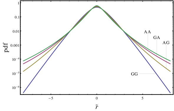
Figure 4: As Fig. 3. Logarithmic scale, abscissa between -8 and +8.

the heavier are the tails, corroborating the construction of our model. In Figs. 5 and 6, we look at the Gaussian–Algebraic case for $K=100$ more closely by varying the dependence on $L$ and $N$. As $L$ is increased for fixed $N=5$, the convergence of the ensemble distribution for the random data matrix to the Gaussian competes with the algebraic tail. Put differently, the exponential tail known from

Figure 5: Probability densities $\langle p\rangle_{GA}^{(k)}$ in the Markovian case versus the rotated amplitudes $\tilde{r}$, normalized to unit standard deviation, $K=100$, $N=5$, $L$ varying as indicated, the smaller $L$, the heavier the tail. Logarithmic scale.

the Gaussian–Gaussian case seems to win for larger $L$. But this is not so, it depends on the range in $\tilde{r}$ considered. On a sufficiently large $\tilde{r}$ scale, the algebraic tail wins.

Figure 6: Probability densities $\langle p\rangle_{GA}^{(k)}$ in the Markovian case versus the rotated amplitudes $\tilde{r}$, normalized to unit standard deviation, $K=100$, $L=65$, $N$ varying as indicated, the smaller $N$, the heavier the tail. Logarithmic scale.

Only in the hard limit $L\rightarrow\infty$ for fixed $\tilde{r}$, there is an exponential tail everywhere. Furthermore, as seen in Fig. 6, the smaller the parameter $N$ for fixed $L=65$, the stronger are the non–stationary fluctuations of the random data matrices. Of course, this must have a large impact on the distribution, but it is interesting to observe that the effect saturates quickly, the curves for $N=9$ and $N=12$ are almost on top of each other.

6 Conclusions

We put forward an approach to model multivariate amplitude distributions in the presence of non–stationarities that imply fluctuations of correlations. This is a frequently encountered situation in complex systems. Our model is based on a division of time scales, the idea behind and the necessary assumption is the existence of a shorter time scale on which the system is in good approximation stationary. Longer time scales are then viewed as assembled from several or many intervals of the shorter time scale. We argued that the correlation or covariance matrices measured in all these shorter time intervals, referred to as epochs, form a truly existing ensemble that we modeled by an ensemble of random matrices. Averaging the multivariate amplitude distributions of the epochs over this ensemble yields heavy tailed amplitude distributions for the larger time scales on which the non–stationarity is crucial. In short, the fluctations of the correlations lift the tails of the multivariate amplitude distributions.

We evaluated our model explicitly for four cases, combining Gaussian and algebraic multivariate amplitude distributions in the epochs with Gaussian and algebraic distributions for the random correlation or covariance matrices. It is a welcome feature that we arrive in all cases at closed form results if the system is Markovian, but even if it is not, the resulting formulae are single integrals. A highly appreciated effect, as in every ensemble approach, is the reduction in the number of relevant parameters. In all of our distributions, there is one parameter that measures the strength with which the correlations fluctuate. Hence, there is a direct measure for the non–stationarity that is obtained by fitting the multivariate distributions to the data. The shape parameters of the algebraic distributions are best determined by fitting the tails. For the distribution for the data in the epochs, the corresponding shape parameters can be obtained before turning to the model on the large time scale.

This discussion also explains why we find simple fit formulae, as often used in finance and referred to as “models”, insufficient. Their parameters neither give a clue on underlying mechanisms nor can they be measured by other means from the data — unlike correlations and covariances. From this point of view, our approach provides justifications of and explanations for fit formulae. Here, we not only gave explicit multivariate distributions for non–stationary systems, but furthermore a tool that quantitatively captures the degree of non–stationarity. Applications to data will be presented in forthcoming studies.

Appendix A Asymptotics of the Ensemble Averaged Amplitude Distributions

We always write $w=\sqrt{r^{\dagger}C^{-1}r}$, we begin with the Gaussian–Algebraic case of Sec. 4.3. To study the integral in Eq. (75), to which we refer as $Q_{GA}$, we write the determinant as Gaussian integral using an $N$ component vector $\zeta$ and employ the power series of the Kummer function

$$Q_{GA} =\int\limits_{0}^{\infty}\frac{\text{d}uu^{K/2-1}}{\sqrt{\det(\mathds{1}_{N}+uD)}}\,_{1}F_{1}\left(L-\frac{N-1}{2},\frac{K}{2},-\frac{Nw^{2}}{2M}u\right)$$

$$=\frac{1}{\pi^{N/2}}\sum\limits_{i=0}^{\infty}\frac{\Gamma(L-(N-1)/2+i)\Gamma(K/2)}{\Gamma(L-(N-1)/2)\Gamma(K/2+i)i!}\left(-\frac{Nw^{2}}{2M}\right)^{i}$$

$$\qquad\qquad\qquad\int\text{d}[\zeta]\exp(-\zeta^{\dagger}\zeta)\int\limits_{0}^{\infty}\text{d}uu^{K/2+i-1}\exp(-u\zeta^{\dagger}D\zeta)\ .$$ (116)

The $u$ integral can now be calculated, and we resum the resulting series

$$Q_{GA} =\frac{\Gamma(K/2)}{\pi^{N/2}}\int\text{d}[\zeta]\exp(-\zeta^{\dagger}\zeta)(\zeta^{\dagger}D\zeta)^{-K/2}\left(1+\frac{Nw^{2}}{2M}\frac{1}{\zeta^{\dagger}D\zeta}\right)^{-L+\frac{N-1}{2}}$$

$$=\frac{\Gamma(K/2)}{\sqrt{\det\pi D}}\left(\frac{Nw^{2}}{2M}\right)^{(N-K)/2}$$

$$\qquad\qquad\int\text{d}[\eta]\exp\left(-\frac{Nw^{2}}{2M}\eta^{\dagger}D^{-1}\eta\right)(\eta^{\dagger}\eta)^{L-(N+K-1)/2}(1+\eta^{\dagger}\eta)^{-L+(N-1)/2}\ ,$$ (117)

where we changed variables according to $\zeta=\sqrt{Nw^{2}/2M}D^{-1/2}\eta$ in the second equation. Introducing hyperspherical coordinates $\eta=\rho e_{\eta}$ with $\text{d}[\eta]=\rho^{N-1}\textrm{d}\rho\textrm{d}\Omega_{N}$ where $\textrm{d}\Omega_{N}$ is the infinitesimal solid angle in $N$ dimensions, we identify the $\rho$ integral as the integral representation (52) of the Tricomi function

$$Q_{GA} =\frac{\Gamma(K/2)\Gamma(L-(K-1)/2)}{2\sqrt{\det\pi D}}\left(\frac{Nw^{2}}{2M}\right)^{(N-K)/2}$$

$$\qquad\qquad\qquad\int U\left(L-\frac{K-1}{2},\frac{N-K}{2}+1,\frac{Nw^{2}}{2M}e_{\eta}^{\dagger}D^{-1}e_{\eta}\right)\textrm{d}\Omega_{N}\ .$$ (118)

The Tricomi function has an asymptotic expansion in its last argument which yields as leading term the inverse of this last argument raised to the power of its first argument. Thus we find

$$\langle p\rangle_{GA}(r|C,D) \longrightarrow\frac{\Gamma(L-(N-1)/2)\Gamma(L-(K-1)/2)}{2\Gamma(L-(K+N-1)/2)\sqrt{\det 2\pi CM/N}\sqrt{\det\pi D}}$$

$$\qquad\qquad\left(\frac{Nw^{2}}{2M}\right)^{-L+\frac{N-1}{2}}\int(e_{\eta}^{\dagger}D^{-1}e_{\eta})^{-L+(K-1)/2}\textrm{d}\Omega_{N}\ .$$ (119)

Most conveniently, the angular average appears only as a factor independent of $w$ and we arrive, as claimed, at the asymptotic behavior (76) of the ensemble averaged amplitude distribution for large $w=\sqrt{r^{\dagger}C^{-1}r}$. Indirectly, this derivation shows that the ensemble avearged amplitude distribution (27) in the case of Gaussian distributed random data matrices cannot be algebraic. As discussed in Sec. 4.3, the limit $L,M\to\infty$ of $\langle p\rangle_{GA}(r|C,D)$ under the condition (65) yields $\langle p\rangle_{GG}(r|C,D)$. This limit, however, is in conflict with the above used asymptotic expansion of the Tricomi function. If such an expansion cannot be applied, the angular average will never separate off as a simple product, seriously hampering a direct derivation of the exponential asymptotics in the Gaussian–Gaussian case for $D\neq\mathds{1}_{N}$.

The algebraic tail in the Algebraic–Gaussian case of Sec. 4.4 is derived accordingly. We notice that in this case, too, the tail in the Markovian situation $D=\mathds{1}_{N}$ immediately follows from the results (76) and (83) due to the above mentioned asymptotic expansion of the Tricomi function which features its last argument to the power of its first argument. With this in mind, we now turn to the Algebraic–Algebraic case of Sec. 4.5. We only consider the Markovian situation $D=\mathds{1}_{N}$ as we may expect that it yields the same asymptotics for the non–Markovian one, too. Thus we consider in the result (91) the hypergeometric function to which we refer as $Q_{AA}$. In the regime $w\gg Mm/N$, we may use the approximation

$$Q_{AA} \simeq{{}_{2}F_{1}}\left(l,L-\frac{N-1}{2},L+l-\frac{K-1}{2},-\frac{Nr^{\dagger}C^{-1}r}{Mm}\right)\ .$$ (120)

An asymptotic expansion can then be infered from the transformation formula [67]

$$\frac{\sin\pi(b-a)}{\pi}\frac{{{}_{2}F_{1}}(a,b,c,z)}{\Gamma(c)}=\frac{(-z)^{-a}}{\Gamma(b)\Gamma(c-a)\Gamma(a-b+1)}{{}_{2}F_{1}}\left(a,a-c+1,a-b+1,\frac{1}{z}\right)$$

$$\qquad\qquad\qquad\qquad-\frac{(-z)^{-b}}{\Gamma(a)\Gamma(c-b)\Gamma(b-a+1)}{{}_{2}F_{1}}\left(b,b-c+1,b-a+1,\frac{1}{z}\right)\ .$$ (121)

The first term in the defining Gauss series of the hypergeometric function is one, implying that the two hypergeometric functions on the right hand side become one for large $z$. The asymptotics is hence determined by $(-z)^{-a}$ or $(-z)^{-b}$, depending on whether $a<b$ or $b>a$. The sine function on the left hand side produces a sign which ensures the positivity of the distribution. To apply this particular line of reasoning to $Q_{AA}$, we must assume that $N$ is even, for odd $N$ cancelations have to prevent the functions $\Gamma(a-b+1)$ and $\Gamma(a-b+1)$ from diverging. If $b=a$, we bring the sine function on the right hand side of Eq. (121) and use l’Hospital’s rule which yields

$${{}_{2}F_{1}}(a,b,c,z) \sim\frac{(-z)^{-a}}{\Gamma(a)\Gamma(c)}\left(1+\frac{\ln(-z)-2\psi(1)-\psi(a)-\psi(c-a)}{\Gamma(c-a)z^{0}}+\ldots\right)\ ,$$ (122)

resulting in a logarithmic correction to the asymptotic behavior. Here $\psi(z)=\Gamma^{\prime}(z)/\Gamma(z)$ is the digamma function.

References

- [1] J. B. Gao. Recurrence Time Statistics for Chaotic Systems and Their Applications. Physical Review Letters, 83:3178–3181, Oct 1999.
- [2] Rainer Hegger, Holger Kantz, Lorenzo Matassini, and Thomas Schreiber. Coping with Nonstationarity by Overembedding. Physical Review Letters, 84:4092–4095, May 2000.
- [3] Pedro Bernaola-Galván, Plamen Ch. Ivanov, Luís A. Nunes Amaral, and H. Eugene Stanley. Scale Invariance in the Nonstationarity of Human Heart Rate. Physical Review Letters, 87:168105, Oct 2001.
- [4] Christoph Rieke, Karsten Sternickel, Ralph G. Andrzejak, Christian E. Elger, Peter David, and Klaus Lehnertz. Measuring Nonstationarity by Analyzing the Loss of Recurrence in Dynamical Systems. Physical Review Letters, 88:244102, May 2002.
- [5] R. Zia and Per Arne Rikvold. Fluctuations and correlations in an individual-based model of biological coevolution. Journal of Physics A, 37, 02 2004.
- [6] R K P Zia and B Schmittmann. A possible classification of nonequilibrium steady states. Journal of Physics A, 39(24):L407–L413, may 2006.
- [7] Jan Pieter Pijn, Jan Van Neerven, André Noest, and Fernando H Lopes da Silva. Chaos or noise in EEG signals; dependence on state and brain site. Electroencephalography and Clinical Neurophysiology, 79(5):371–381, 1991.
- [8] Markus Müller, Gerold Baier, Andreas Galka, Ulrich Stephani, and Hiltrud Muhle. Detection and characterization of changes of the correlation structure in multivariate time series. Physical Review E, 71:046116, Apr 2005.
- [9] R. Höhmann, U. Kuhl, H.-J. Stöckmann, L. Kaplan, and E. J. Heller. Freak Waves in the Linear Regime: A Microwave Study. Physical Review Letters, 104:093901, Mar 2010.
- [10] Jakob J. Metzger, Ragnar Fleischmann, and Theo Geisel. Statistics of Extreme Waves in Random Media. Physical Review Letters, 112:203903, May 2014.
- [11] Henri Degueldre, Jakob Metzger, Theo Geisel, and Ragnar Fleischmann. Random Focusing of Tsunami Waves. Nature Physics, 12, 11 2015.
- [12] Geert Bekaert and Campbell R. Harvey. Time-Varying World Market Integration. Journal of Finance, 50(2):403–444, 1995.
- [13] Francois Longin and Bruno Solnik. Is the correlation in international equity returns constant: 1960-1990? Journal of International Money and Finance, 14(1):3–26, 1995.
- [14] J.-P. Onnela, A. Chakraborti, K. Kaski, J. Kertész, and A. Kanto. Dynamics of market correlations: Taxonomy and portfolio analysis. Physical Review E, 68:056110, Nov 2003.
- [15] Yiting Zhang, Gladys Hui Ting Lee, Jian Cheng Wong, Jun Liang Kok, Manamohan Prusty, and Siew Ann Cheong. Will the US economy recover in 2010? A minimal spanning tree study. Physica A, 390(11):2020–2050, 2011.
- [16] Dong-Ming Song, Michele Tumminello, Wei-Xing Zhou, and Rosario N. Mantegna. Evolution of worldwide stock markets, correlation structure, and correlation-based graphs. Physical Review E, 84:026108, Aug 2011.
- [17] Leonidas Sandoval and Italo De Paula Franca. Correlation of financial markets in times of crisis. Physica A, 391(1):187–208, 2012.
- [18] Michael C. Münnix, Takashi Shimada, Rudi Schäfer, Francois Leyvraz, Thomas H. Seligman, Thomas Guhr, and H. Eugene Stanley. Identifying States of a Financial Market. Scientific Reports, 2:644, Sep 2012.
- [19] F. Ghasemi, Muhammad Sahimi, Joachim Peinke, and M Tabar. Analysis of Non-stationary Data for Heart-Rate Fluctuations in Terms of Drift and Diffusion Coefficients. Journal of Biological Physics, 32:117–28, 11 2006.
- [20] Mehrnaz Anvari, Cina Aghamohammadi, H. Dashti-Naserabadi, E. Salehi, E. Behjat, M. Qorbani, M. Khazaei Nezhad, M. Zirak, Ali Hadjihosseini, Joachim Peinke, and M. Reza Rahimi Tabar. Stochastic nature of series of waiting times. Physical Review E, 87:062139, Jun 2013.
- [21] Fatemeh Ghasemi, Muhammad Sahimi, J. Peinke, R. Friedrich, G. Reza Jafari, and M. Reza Rahimi Tabar. Markov analysis and Kramers-Moyal expansion of nonstationary stochastic processes with application to the fluctuations in the oil price. Physical Review E, 75:060102, Jun 2007.
- [22] Rudi Schäfer and Thomas Guhr. Local normalization: Uncovering correlations in non-stationary financial time series. Physica A, 389(18):3856–3865, 2010.
- [23] A. Bohr and B.R. Mottelson. Nuclear Structure: Volume 2, Nuclear deformations. Nuclear Structure. Benjamin, 1969.
- [24] Vladimir Zelevinsky. Quantum Chaos and Complexity in Nuclei. Annual Review of Nuclear and Particle Science, 46(1):237–279, 1996.
- [25] Thomas Guhr, Axel Müller-Groeling, and Hans A. Weidenmüller. Random Matrix Theories in Quantum Physics: Common Concepts. Physics Reports, 299:189–425, 1998.
- [26] Thilo A. Schmitt, Desislava Chetalova, Rudi Schäfer, and Thomas Guhr. Non-stationarity in financial time series: Generic features and tail behavior. Europhysics Letters, 103(5):58003, 2013.
- [27] Frederik Meudt, Martin Theissen, Rudi Schäfer, and Thomas Guhr. Constructing Analytically Tractable Ensembles of Non-Stationary Covariances with an Application to Financial Data. Journal of Statistical Mechanics, 2015(11):P11025, 03 2015.
- [28] Thilo Schmitt, Desislava Chetalova, Rudi Schäfer, and Thomas Guhr. Credit Risk and the Instability of the Financial System: an Ensemble Approach. Europhysics Letters, 105, 09 2013.
- [29] Thilo Schmitt, Rudi Schäfer, and Thomas Guhr. Credit Risk: Taking Fluctuating Asset Correlations into Account. Journal of Credit Risk, 11:73–94, 09 2015.
- [30] Rudi Schäfer, Sonja Barkhofen, Thomas Guhr, Hans-Jürgen Stöckmann, and Ulrich Kuhl. Compounding Approach for Univariate Time Series with Nonstationary Variances. Physical Review E, 92:062901, Dec 2015.
- [31] Satya Dubey. Compound gamma, beta and F distributions. Metrika: International Journal for Theoretical and Applied Statistics, 16(1):27–31, 1970.
- [32] O. Barndorff-Nielsen, J. Kent, and M. Sørensen. Normal Variance-Mean Mixtures and z Distributions. International Statistical Review / Revue Internationale de Statistique, 50(2):145–159, 1982.
- [33] C. Beck and E.G.D. Cohen. Superstatistics. Physica A, 322(C):267–275, 2003.
- [34] A. Y. Abul-Magd, G. Akemann, and P. Vivo. Superstatistical generalizations of Wishart–Laguerre ensembles of random matrices. Journal of Physics A, 42(17):175207, 2009.
- [35] Anthony Paul Doulgeris and Torbjørn Eltoft. Scale Mixture of Gaussian Modelling of Polarimetric SAR Data. EURASIP Journal on Advances in Signal Processing, 2010, 2010.
- [36] Florence Forbes and Darren Wraith. A new family of multivariate heavy-tailed distributions with variable marginal amounts of tailweight: Application to robust clustering. Statistics and Computing, 24, 11 2014.
- [37] JP Bouchaud and M Potters. Theory of Financial Risks, From Statistical Physics to Risk Management. Cambridge University Press, New York, 2000.
- [38] M.L. Mehta. Random Matrices. ISSN. Elsevier Science, 2004.
- [39] J. Wishart. The Generalised Product Moment Distribution in Samples From a Normal Multivariate Population. Biometrika, 20A(1-2):32–52, 1928.
- [40] Laurent Laloux, Pierre Cizeau, Jean-Philippe Bouchaud, and Marc Potters. Noise Dressing of Financial Correlation Matrices. Physical Review Letters, 83:1467–1470, Aug 1999.
- [41] Laurent Laloux, Pierre Cizeau, Marc Potters, and Jean-Philippe Bouchaud. Random Matrix Theory and Financial Correlations. International Journal of Theoretical and Applied Finance, 03(03):391–397, 2000.
- [42] Vasiliki Plerou, Parameswaran Gopikrishnan, Bernd Rosenow, Luís A. Nunes Amaral, and H. Eugene Stanley. Universal and Nonuniversal Properties of Cross Correlations in Financial Time Series. Physical Review Letters, 83:1471–1474, Aug 1999.
- [43] Vasiliki Plerou, Parameswaran Gopikrishnan, Bernd Rosenow, Luis A. Nunes Amaral, Thomas Guhr, and H. Eugene Stanley. Random Matrix Approach to Cross Correlations in Financial Data. Physical Review E, 65:066126, Jun 2002.
- [44] Szilárd Pafka and Imre Kondor. Estimated correlation matrices and portfolio optimization. Physica A, 343(C):623–634, 2004.
- [45] Marc Potters, Jean-Philippe Bouchaud, and Laurent Laloux. Financial Applications of Random Matrix Theory: Old Laces and New Pieces. Acta Physica Polonica B, 36:2767–2784, 09 2005.
- [46] S Drozdz, J Kwapien, and P Oswiecimka. Empirics Versus RMT in Financial Cross-Correlations. Acta Physica Polonica B, 39(1):4027–4039, 2008.
- [47] Jaroslaw Kwapien, Stanislaw Drozdz, and P. Oswiecimka. The bulk of the stock market correlation matrix is not pure noise. Physica A, 359:589–606, 05 2006.
- [48] Giulio Biroli, Jean-Philippe Bouchaud, and Marc Potters. The Student ensemble of correlation matrices: eigenvalue spectrum and Kullback-Leibler entropy. Acta Physica Polonica B, 38:4009–4026, 10 2007.
- [49] Zdzislaw Burda, J. Jurkiewicz, Maciej Nowak, Gábor Papp, and Ismail Zahed. Free Levy Matrices and Financial Correlations. Physica A, 343:694–700, 04 2001.
- [50] Zdzisław Burda, Romuald A. Janik, Jerzy Jurkiewicz, Maciej A. Nowak, Gabor Papp, and Ismail Zahed. Free random Lévy matrices. Physical Review E, 65:021106, Jan 2002.
- [51] Gernot Akemann and Pierpaolo Vivo. Power law deformation of Wishart–Laguerre ensembles of random matrices. Journal of Statistical Mechanics, 2008(09):P09002, 2008.
- [52] Zdzislaw Burda, Andrzej Jarosz, Maciej A. Nowak, Jerzy Jurkiewicz, Gábor Papp, and Ismail Zahed. Applying free random variables to random matrix analysis of financial data. Part I: The Gaussian case. Quantitative Finance, 11(7):1103–1124, Jul 2011.
- [53] J.B. French, P.A. Mello, and A. Pandey. Ergodic behavior in the statistical theory of nuclear reactions. Physics Letters B, 80:17–19, 1978.
- [54] R. U. Haq, A. Pandey, and O. Bohigas. Fluctuation Properties of Nuclear Energy Levels: Do Theory and Experiment Agree? Physical Review Letters, 48:1086–1089, Apr 1982.
- [55] J.J.M. Verbaarschot and T. Wettig. Random Matrix Theory and Chiral Symmetry in QCD. Annual Review of Nuclear and Particle Science, 50(1):343–410, 2000.
- [56] P.C. Mahalanobis. On the generalised distance in statistics. Proceedings of the National Institute of Science of India, 2:49–55, 1936.
- [57] Steven H. Simon and Aris L. Moustakas. Eigenvalue density of correlated complex random Wishart matrices. Physical Review E, 69:065101, Jun 2004.
- [58] Zdzisław Burda, Jerzy Jurkiewicz, and Bartłomiej Wacław. Spectral moments of correlated Wishart matrices. Physical Review E, 71:026111, Feb 2005.
- [59] M. R. McKay, A. J. Grant, and I. B. Collings. Performance Analysis of MIMO-MRC in Double-Correlated Rayleigh Environments. IEEE Transactions on Communications, 55(3):497–507, 2007.
- [60] Daniel Waltner, Tim Wirtz, and Thomas Guhr. Eigenvalue Density of the Doubly Correlated Wishart Model: Exact Results. Journal of Physics A, 48:175204, 12 2014.
- [61] Zdzislaw Burda and Jerzy Jurkiewicz. Chapter 13, Heavy-tailed Random Matrices. In Gernot Akemann, Jinho Baik, and Philippe Di Francesco, editors, Oxford Handbook of Random Matrix Theory, page 270. Oxford University Press, 09 2015.
- [62] Peter Forrester and Manjunath Krishnapur. Derivation of an eigenvalue probability density function relating to the Poincare disk. Journal of Physics A, 42, 2009.
- [63] Tim Wirtz, Daniel Waltner, Mario Kieburg, and Santosh Kumar. The Correlated Jacobi and the Correlated Cauchy-Lorentz ensembles. Journal of Statistical Physics, 162:495, 01 2016.
- [64] Thomas Guhr and Andreas Schell. Matrix Moments in a Real, Doubly Correlated Algebraic Generalization of the Wishart Model. submitted for publication, 2020.
- [65] Carl Ludwig Siegel. Über Die Analytische Theorie Der Quadratischen Formen. Annals of Mathematics, 36(3):527–606, 1935.
- [66] Yan V. Fyodorov. Negative moments of characteristic polynomials of random matrices: Ingham–Siegel integral as an alternative to Hubbard–Stratonovich transformation. Nuclear Physics B, 621(3):643–674, Jan 2002.
- [67] I.S. Gradsteyn and I.M.Ryzhik. Table of Integrals, Series, and Products. Academic Press, 7 edition, 2007.