Understanding Climate Impacts on Vegetation with Gaussian Processes in Granger Causality

Abstract

Global warming is leading to unprecedented changes in our planet, with great societal, economical and environmental implications, especially with the growing demand of biofuels and food. Assessing the impact of climate on vegetation is of pressing need. We approached the attribution problem with a novel nonlinear Granger causal (GC) methodology and used a large data archive of remote sensing satellite products, environmental and climatic variables spatio-temporally gridded over more than 30 years. We generalize kernel Granger causality by considering the variables cross-relations explicitly in Hilbert spaces, and use the covariance in Gaussian processes. The method generalizes the linear and kernel GC methods, and comes with tighter bounds of performance based on Rademacher complexity. Spatially-explicit global Granger footprints of precipitation and soil moisture on vegetation greenness are identified more sharply than previous GC methods.

1 Introduction

Establishing causal relations between random variables from observational data is perhaps the most important challenge in today’s science in general and in Earth sciences in particular [1]. Granger causality (GC) [2] was introduced as a first attempt to formalize quantitatively the causal relation between time series, and is the most widely used method. The intuition behind GC is to test whether the past of $X$ helps in predicting the future of $Y$ from its past alone. GC implicitly tells us about the concept of information using forecasting. Other methods rely on similar concepts of information flow and predictability: connections can be established between GC and transfer entropy [3], convergent cross-mapping [4], and with the graphical causal model perspective [5]. Noting the strong linearity assumption in GC [6], nonlinear extensions of GC have been proposed. In particular, GC with kernels was originally introduced in [7]. The method assumed a particular class of functions and an additive interaction between them. An alternative kernel-based test in combination with a filtering approach was later introduced in [8]. In all these studies, the autoregressive (AR) models use kernel-based regression on the concatenation of the involved variables in input spaces. This approach, however, is limited as it disregards nonlinear cross-relations between $X$ and $Y$ in Hilbert spaces explicitly. We here introduce explicit feature maps and corresponding kernel functions that account for nonlinear cross-relations in kernel space [9].

2 Crosskernel Gaussian processes for Granger Causality

GC first builds univariate and bivariate AutoRegressive (AR) models: (1) $y_{t+1}={\bf a}_{t}^{\intercal}{\bf y}_{t}+\varepsilon_{t}^{y}$ and (2) $y_{t+1}={\bf a}_{t}^{\intercal}{\bf y}_{t}+{\bf b}_{t}^{\intercal}{\bf x}_{t}+\varepsilon_{t}^{y|x}$, where ${\bf y}_{t}=[y_{t},y_{t-1},\ldots,y_{t-P}]^{\intercal}$, ${\bf x}_{t}=[x_{t},x_{t-1},\ldots,x_{t-Q}]^{\intercal}$, and ${\bf a}=[a_{1},\ldots,a_{P}]^{\intercal}$ and ${\bf b}=[b_{1},\ldots,b_{Q}]^{\intercal}$ are typically estimated by least squares. A GC test is defined as the ratio of model fitting errors: $\delta_{x\to y}=\log({\mathbb{V}}[\varepsilon_{t}^{y}]/{\mathbb{V}}[\varepsilon_{t}^{y|x}])$, where the residual errors are defined for the unrestricted $\varepsilon_{t}^{y}$ and restricted $\varepsilon_{t}^{y|x}$ cases separately, and ${\mathbb{V}}$ represents the variance operator. Conditional Granger causality traditionally considers incrementing the variable ${\bf y_{t}}$ by stacking the variables one conditions to ${\bf z}$, that is ${\bf y_{t}}^{\prime}:=[{\bf y_{t}},{\bf z_{t}}]$, and applying the same methodology. The linear GC formulation can be generalized to the nonlinear case using elements of the theory of reproducing kernel Hilbert spaces (RKHS) [10]. Let us assume the existence of a Hilbert space $\mathcal{H}$ equipped with an inner product where samples in $\mathcal{X}$ are mapped into by means of a feature map $\bm{\mathit{\phi}}:\mathcal{X}\to\mathcal{H},{\bf x}_{i}\mapsto\bm{\mathit{\phi}}({\bf x}_{i})$, $1\leq i\leq n$. The similarity between the elements in $\mathcal{H}$ can be estimated using its associated dot product $\langle\cdot,\cdot\rangle_{\mathcal{H}}$ via RKHS, $k:\mathcal{X}\times\mathcal{X}\to\mathbb{R}$, such that $({\bf x},{\bf x}^{\prime})$ $\mapsto$ $k({\bf x},{\bf x}^{\prime})$.

Stacked kernel. The standard kernel GC (KGC) approach considers a kernel-based AR modeling [8, 7]. The method defines two feature maps $\bm{\phi}$ and $\bm{\psi}$ to a RKHS ${\mathcal{H}}$ endorsed with reproducing kernels $k$ and $\ell$, where ${\bf y}_{t}$ and the concatenation ${\bf z}_{t}=[{\bf y}_{t},{\bf x}_{t}]\in^{P+Q}$ are mapped to, respectively. This leads to the kernel regression models (1) $y_{t+1}={\bf a}_{H}^{\intercal}\bm{\mathit{\phi}}({\bf y}_{t})+\varepsilon_{t}^{y}$ and (2) $y_{t+1}={\bf b}_{H}^{\intercal}\bm{\mathit{\psi}}({\bf z}_{t})+\varepsilon_{t}^{y|x}$, where now ${\bf a}_{H},{\bf b}_{H}\in^{H\times 1}$. By using the representer’s theorems ${\bf a}_{H}=\bm{\Phi}^{\intercal}\bm{\alpha}$ and ${\bf b}_{H}=\bm{\Psi}^{\intercal}\bm{\beta},$ where $\bm{\Phi},\bm{\Psi}\in^{n\times H}$, the AR models can be defined in terms of kernel functions only: $y_{t+1}=\bm{\alpha}^{\intercal}{\bf k}_{t}+\varepsilon_{t}^{y}$, and $y_{t+1}=\bm{\beta}^{\intercal}\bm{\ell}_{t}+\varepsilon_{t}^{y|x}$, respectively, where ${\bf k}_{t}=[k({\bf y}_{1},{\bf y}_{t}),\ldots,k({\bf y}_{n},{\bf y}_{t})]^{\intercal}$ and $\bm{\ell}_{t}=[\ell({\bf z}_{1},{\bf z}_{t}),\ldots,\ell({\bf z}_{n},{\bf z}_{t})]^{\intercal}$ contain all evaluations of $k$ and $\ell$ at time $t$. Since data are mapped to the same Hilbert space ${\mathcal{H}}$, the same kernel function and parameters are used for both $k$ and $\ell$.

Summation kernel. Alternatively implicit AR models can be defined in RKHS [7]: $y_{t+1}={\bf a}_{H}^{\intercal}\bm{\mathit{\phi}}({\bf y}_{t})+\varepsilon_{t}^{y}$, and $y_{t+1}={\bf a}_{H}^{\intercal}\bm{\mathit{\phi}}({\bf y}_{t})+{\bf b}_{H}^{\intercal}\bm{\mathit{\psi}}({\bf x}_{t})+\varepsilon_{t}^{y|x},$ which leads to the kernel AR models $y_{t+1}=\alpha^{\intercal}{\bf k}_{t}+\varepsilon_{t}^{y}$ and $y_{t+1}=\alpha^{\intercal}{\bf k}_{t}+\beta^{\intercal}\bm{\ell}_{t}+\varepsilon_{t}^{y|x},$ where now $\bm{\ell}_{t}:=[\ell({\bf x}_{1},{\bf x}_{t}),\ldots,\ell({\bf x}_{n},{\bf x}_{t})]^{\intercal}$. The summation kernel is more appropriate when large time embeddings $P$ and $Q$ are needed to capture long-term memory processes, since it avoids constructing large dimensional feature vectors ${\bf z}$ by concatenation. However, the cross-information between $X$ and $Y$ is missing.

Explicit cross-kernel. In order to account for cross-correlations in Hilbert space, while alleviating the issue of large embeddings in conditional GC setups. we propose to explicitly define two feature maps: the standard individual map $\phi$ and the joint feature mapping $\psi$ for the second AR model: $y_{t+1}={\bf a}_{H}^{\intercal}\bm{\phi}({\bf y}_{t})+\varepsilon_{t}^{y}$ and $y_{t+1}={\bf b}_{H}^{\intercal}\bm{\psi}({\bf x}_{t},{\bf y}_{t})+\varepsilon_{t}^{y|x}$, where the joint map is defined by construction as $\widetilde{\bm{\psi}}({\bf x}_{t},{\bf y}_{t}):=[{\bf A}_{1}\bm{\varphi}({\bf y}_{t}),{\bf A}_{2}\bm{\varphi}({\bf x}_{t}),{\bf A}_{3}(\bm{\varphi}({\bf y}_{t})+\bm{\varphi}({\bf x}_{t}))]^{\intercal},$ where $\bm{\varphi}$ is a nonlinear feature map into an RKHS ${\mathcal{H}}$, and ${\bf A}_{i}$, $i=1,2,3$, are three linear transformations from ${\mathcal{H}}$ to ${\mathcal{H}}_{i}$. The induced joint kernel function readily becomes:

$$\begin{array}[]{ll}&n(({\bf x}_{t},{\bf y}_{t}),({\bf x}_{t}^{\prime},{\bf y}_{t}^{\prime}))=\widetilde{\bm{\psi}}({\bf x}_{t},{\bf y}_{t})^{\intercal}\widetilde{\bm{\psi}}({\bf x}_{t}^{\prime},{\bf y}_{t}^{\prime})\\ &\hskip 28.45274pt=\bm{\varphi}({\bf y}_{t})^{\intercal}{\bf R}_{1}\bm{\varphi}({\bf y}_{t}^{\prime})+\bm{\varphi}({\bf x}_{t})^{\intercal}{\bf R}_{2}\bm{\varphi}({\bf x}_{t}^{\prime})+\bm{\varphi}({\bf y}_{t})^{\intercal}{\bf R}_{3}\bm{\varphi}({\bf x}_{t}^{\prime})+\bm{\varphi}({\bf x}_{t})^{\intercal}{\bf R}_{3}\bm{\varphi}({\bf y}_{t}^{\prime})\\ &\hskip 28.45274pt=\!n_{1}({\bf y}_{t},{\bf y}_{t}^{\prime})\!+\!n_{2}({\bf x}_{t},{\bf x}_{t}^{\prime})\!+\!n_{3}({\bf y}_{t},{\bf x}_{t}^{\prime})\!+\!n_{4}({\bf x}_{t},{\bf y}_{t}^{\prime}),\end{array}$$ (4)

where ${\bf R}_{1}={\bf A}_{1}^{\intercal}{\bf A}_{1}+{\bf A}_{3}^{\intercal}{\bf A}_{3}$, ${\bf R}_{2}={\bf A}_{2}^{\intercal}{\bf A}_{2}+{\bf A}_{3}^{\intercal}{\bf A}_{3}$, and ${\bf R}_{3}={\bf A}_{3}^{\intercal}{\bf A}_{3}$. The new kernel function considers cross-terms relations between the time series through kernels $n_{3}$ and $n_{4}$. Besides, there is no need to explicitly use the same kernel function or parameters, and can be convenient to alleviate the problem of increased dimensionality in conditional GC settings as ours.

We used the previous kernel/covariance in Gaussian Processes (GPs) [11]. The GP modeling of XKGC assumes that the AR functions $\mathbf{f}_{y}$ and $\mathbf{f}_{y|x}$ follow $n$-dimensional Gaussian distributions $\mathbf{f}_{y},\sim\mathcal{N}({\bf 0},{\bf K})$ and $\mathbf{f}_{y|x}\sim\mathcal{N}({\bf 0},{\bf L})$, and covariances ${\bf K}$ and ${\bf L}$ (or respectively ${\bf N}$) of the distributions are determined by a kernel function. A direct sum of covariances is also a covariance so all kernel functions in the XKGC framework ($k$, $l$ and $n$) induce valid GPs. The XKGC allows to advantageously optimize hyperparameters by Type-II Maximum Likelihood using the marginal likelihood of the observations. The GP treatment also permits to define a test statistic based on the the evidence. We suggest the GC criterion for the GP versions as follows:

$$\delta^{\text{GP}}_{x\to y}=\max_{\bm{\theta}_{2}}\log(p_{2}({\bf f}_{y}|X,Y))-\max_{\bm{\theta}_{1}}\log(p_{1}({\bf f}_{y}|Y)),$$

which represents the difference between log-evidences of the two GP AR models, so we infer $X\to Y$ when the evidence of conditioned model is larger than the evidence of the unconditioned model.

The cross-kernel GC (XKGC) generalizes previous KGC methods and comes with statistical guarantees when used in GPs. Owing to the connection between GPs and KRR [12], our GP model function class $h$ implicitly uses the squared loss for $\widehat{R}(h)$. Let us use an squared exponential kernel, $k({\bf x},{\bf x})=1$, and let $\gamma\in[0,1]$ and $\beta\in[\gamma,1]$. The Rademacher complexity regression minimum bound for the cross-kernel is:

$$R_{\text{cross}}(h)\leq\widehat{R}(h)+\frac{8\|h\|^{2}}{\sqrt{n}}\left(\sqrt{\frac{1+\gamma}{1+\beta}}+\frac{3}{4}\sqrt{\frac{\log(2/\delta)}{2}}\right),$$

which follows from the Rademacher complexity for a sum of $N$ kernels $K_{i}$ can be easily bounded as $\widehat{R}(h)=\sqrt{N}\widehat{R}(h_{i})$, $i=1,\ldots,N$; $M^{2}=2(1+\beta)$ and the Tr$[{\bf K}]=2n(1+\gamma)$ for the cross-kernel. For the stacked kernel, $M^{2}=1$ and Tr$[{\bf K}]=n$, and for the summation $M^{2}=2$ and Tr$[{\bf K}]=2n$, we obtain $R_{\text{cross}}(h)\leq R_{\text{sum}}(h)=R_{\text{stacked}}$. Note that for $\gamma=\beta$, i.e. when $X$ and $Y$ convey correlated information, the cross-kernel bound converges to the stacked and the summation bounds. Since $\gamma\leq\beta$, the cross-kernel bound will be always tighter than the stacked/summation kernel bound.

3 Experimental results

3.1 Data collection and preprocessing

Our study used the database in [13] available at https://sat-ex.ugent.be/, which consists of climatic data obtained from both satellite observations and in-situ measurements. Variables are classified into four categories of driving forcings: temperature, precipitation, soil moisture, and radiation. A total of $18$ different products are available, and span over $1981-2010$ on a global scale. Data were converted to a common monthly temporal resolution and $1º\times 1º$ latitude-longitude of spatial resolution, and $13072$ (pixel) time series were processed, see Appendix.

The application of Granger causality requires stationary data so we removed the trend and periodicity of all time series. Both are confounding factors that inflate Granger detection. The seasonal cycle was estimated as the average annual mean over the $30$ years, and subtracted from the raw time series to yield time series of anomalies. Variable selection was also very relevant. We selected one product per variable. For this, a correlation study was carried out between all products with the NDVI product. A maximum vote strategy was deployed on the results of Pearson’s, Spearman’s and Kendall’s correlation coefficients. This yielded a database of four predictor variables (temperature, precipitation, soil moisture and radiation) corresponding to the anomalies of the four categories. We performed the study with data from coincident months. Data standardization was applied to all series. Granger causality was then carried out using one variable at a time and conditioning on the others. Our target variable is NDVI that accounts for vegetation greenness. We compare the detection ability and class-specificity of the standard Vector Autoregressive (VAR) model, Gaussian Process (GP) and the proposed cross-kernel Gaussian Process (XKGP). All $13072$ models were cross-validated.

3.2 Detection, robustness and class-specificity

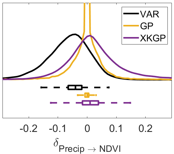
Figure 1: Density of global $\delta$ values between precipitation and NDVI.

Figure 1 shows the global densities of $\delta$ values obtained for each regression model in the particular case of precipitation$\to$greenness (similar results were obtained for the case of soil moisture). The VAR model shows very poor detections globally (negative mean and heavy tail skewed over negative values) which indicates it is unable to find the causal relation in most of the pixels. The pathological case of standard GP indicates that the vast majority of decisions are slightly positive, yet close to zero, and the density is symmetric so detection is fairly compromised. The proposed XKGP leads to improved results over both VAR and GPs, with a clear positive mean and larger variability Granger-causal detections.

The results are analyzed per biome type for precipitation and soil moisture as driving forces in Table 1. The dominant capabilities of XKGP are obvious in both forcings (bold faced). Precipitation impacts greenness and XKGP finds stronger detections in shrublands, savannas and herbaceous (highlighted in italics), indicating enhanced detection capabilities in water-limited biomes. Similar results are observed when considering SM as the driver (conditioned to temperature, radiation and precipitation too). The lowest $\delta$ detections were obtained for forests, especially for needle-leaf and evergreen forests, as expected.

Table 1: Mean $\delta$ and standard error ($\times$100) per IGBP land cover class and model for precip and SM.

	Precipitation			Soil moisture
	VAR	GP	XKGP	VAR	GP	XKGP
Needleleaf Forest	-6.2 $\pm$ 0.4	0.0 $\pm$ 0.1	0.3 $\pm$ 0.4	-6.2 $\pm$ 0.5	0.06 $\pm$ 0.04	0.9 $\pm$ 0.4
Evergreen Broadleaf Forest	-7.4 $\pm$ 0.2	-0.1 $\pm$ 0.1	0.8 $\pm$ 0.3	-7.3 $\pm$ 0.3	0.3 $\pm$ 0.1	1.9 $\pm$ 0.3
Deciduous Broadleaf Forest	-7.0 $\pm$ 1.0	-0.1 $\pm$ 0.1	0.7 $\pm$ 0.5	-9.0 $\pm$ 1.0	-0.1 $\pm$ 0.2	2.0 $\pm$ 1.0
Mixed Forest	-6.3 $\pm$ 0.4	0.0 $\pm$ 0.1	1.2 $\pm$ 0.4	-6.6 $\pm$ 0.4	0.1 $\pm$ 0.1	2.8 $\pm$ 0.4
Shrublands	-4.2 $\pm$ 0.3	1.4 $\pm$ 0.3	4.1 $\pm$ 0.7	-2.7 $\pm$ 0.4	2.4 $\pm$ 0.3	5.1 $\pm$ 0.6
Savannas	-3.6 $\pm$ 0.6	0.8 $\pm$ 0.3	5.9 $\pm$ 0.9	-5.3 $\pm$ 0.6	0.6 $\pm$ 0.3	5.9 $\pm$ 0.8
Herbaceous	-2.9 $\pm$ 0.7	1.7 $\pm$ 0.6	6.8 $\pm$ 0.9	-3.9 $\pm$ 0.4	1.0 $\pm$ 0.2	7.1 $\pm$ 0.9
Cultivated	-5.4 $\pm$ 0.4	0.0 $\pm$ 0.2	3.2 $\pm$ 0.6	-4.3 $\pm$ 0.4	0.3 $\pm$ 0.1	6.8 $\pm$ 0.7

3.3 Global footprints of precipitation and moisture on vegetation

Let us now look at global and regional scales in Fig. 2. The gradient maps show where precipitation or moisture become more relevant for VAR (left) and GP (right). Overall, one can see many (spurious) detections of VAR, which cannot cope with the well-known nonlinear processes involved as reported in [13]. This can be better observed in the regional maps of Africa and Australia, where the GP model yields sharper and clearer detections spatially. This suggests that the variability of central Africa, among other areas, obtained through VAR may be an artifact of the model. It is worth noting that areas detected with high GC impact correspond to those related to El Niño Southern Oscillation (ENSO) event, which causes droughts in the south-east of Africa and the east coast of Australia.

Results show that Granger-climatic dynamics cause vegetation anomalies over most of the continental surface, with a greater impact in subtropical regions and mid-latitudes. Water availability is the main factor driving NDVI anomalies worldwide, finding a great Granger-causal relationship in semi-arid areas or in areas where a large part of vegetation dynamics responds to rainfall. In general, our findings highlight a strong dependence of global vegetation on water availability and show the effect of hydroclimatic anomalies on global vegetation over the studied period. These results suggest that vegetation is susceptible to follow future trends in water availability, and nonlinear (Granger) causal methods can capture this and quantify it adequately. These results suggest that vegetation will be critically influenced by the effect of climate warming on water-limited regions.

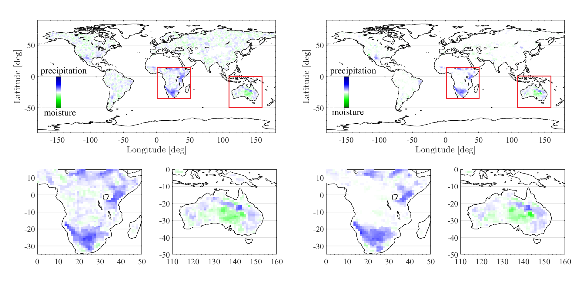
Figure 2: Global Granger footprint maps of precipitation and humidity on vegetation using VAR (left) and GP (right), with zoomed areas over Africa and Australia (bottom).

4 Conclusions

We considered Granger causality and its wide adoption and applicability in Earth sciences. Noting the main shortcomings of stationarity and linearity, we proposed a kernel-based framework that generalizes previous linear and kernel GC approaches. The methodology copes with nonlinear relationships more efficiently and comes with statistical guarantees. The application on assessing the impact of climate variables on vegetation status and health summarized by vegetation indices suggested sharper and more robust Granger detection capabilities compared to previous methods.

Appendix. Data collection and availability

Table 2: Data sets used in the analysis. These data sets are used to construct predictive features for the non-linear Granger causality framework. The NDVI is used to derive the target variable.

Variable	Dataset	Spatial resolution	Temporal resolution	Reference
Temperature	CRU-HR	0.5º	monthly	Harris et al, 2014 [14]
	UDel	0.5º	monthly	Willmott y Matsuura, 2001 [15]
	ISCCP	1º	daily	Rossow y Duenas, 2004 [16]
	ERA-Interim	0.75º	3- hourly	Dee et al, 2011 [17]
	GISS	2º	monthly	Hansen et al, 2013 [18]
	MLOST	5º	monthly	Smith et al, 2008 [19]
	CFSR-Land	0.5º	daily	Coccia et al, 2015 [20]
Precipitation	CRU-HR	0.5º	monthly	Harris et al, 2014 [14]
	UDel	0.5º	monthly	Willmott y Matsuura, 2001 [15]
	CPC-U	0.25º	daily	Xie et al, 2007 [21]
	GPCC	0.5º	monthly	Schneider et al, 2016 [22]
	CMAP	2.5º	monthly	Xie y Arkin, 1997 [23]
	GPCP	2.5º	monthly	Adler et al, 2003 [24]
	MSWEP	0.25º	3- hourly	Beck et al, 2017 [25]
Soil moisture	GLEAM	0.25º	daily	Miralles et al, 2011 [26]
Radiation	SRB	1º	3- hourly	Stackhouse et al, 2004 [27]
	ERA-Interim	0.75º	3- hourly	Dee et al, 2011 [17]
NDVI	GIMMS	0.25º	monthly	Tucker et al, 2005 [28]

References

- [1] J. Runge, S. Bathiany, E. Bollt, G. Camps-Valls, D. Coumou, E. Deyle, C. Clymour, M. Kretschmer, M. Mahecha, J. Muñoz-Marí, E. van Nes, J. Peters, R. Quax, M. Reichstein, M. Scheffer, B. Schölkopf, P. Spirtes, G. Sugihara, J. Sun, K. Zhang, and J. Zscheischler. Inferring causation from time series with perspectives in Earth system sciences. Nature Communications, 10(2553), 2019.
- [2] C. W. J. Granger. Investigating causal relations by econometric models and cross-spectral methods. Econometrica, 37(3):424–438, 1969.
- [3] Thomas Schreiber. Measuring information transfer. Phys. Rev. Lett., 85:461–464, Jul 2000.
- [4] G. Sugihara, R. May, H. Ye, C.-h. Hsieh, E. Deyle, M. Fogarty, and S. Munch. Detecting causality in complex ecosystems. Science, 338(6106):496–500, 2012.
- [5] Halbert White, Karim Chalak, Xun Lu, and others. Linking Granger Causality and the Pearl Causal Model with Settable Systems. In NIPS Mini-Symposium on Causality in Time Series, pages 1–29, 2011.
- [6] Michael Eichler. Causal inference from time series: What can be learned from Granger causality. In Proc. Intnl. Cong. Logic, Methodology and Philosophy of Science, pages 1–12, 2007.
- [7] Nicola Ancona, Daniele Marinazzo, and Sebastiano Stramaglia. Radial basis function approach to nonlinear Granger causality of time series. Phys. Rev. E, 70:056221, Nov 2004.
- [8] Daniele Marinazzo, Mario Pellicoro, and Sebastiano Stramaglia. Kernel method for nonlinear Granger causality. Phys. Rev. Lett., 100:144103, Apr 2008.
- [9] M. Martínez-Ramón, J. L. Rojo-Álvarez, G. Camps-Valls, A. Navia-Vázquez, E. Soria-Olivas, and A. R. Figueiras-Vidal. Support vector machines for nonlinear kernel ARMA system identification. IEEE Trans. Neur. Networks, 17(6):1617–1622, 2007.
- [10] Nello Cristianini and Bernhard Schölkopf. Support vector machines and kernel methods: The new generation of learning machines. AI Mag., 23(3):31–41, September 2002.
- [11] C. E. Rasmussen and C. K. I. Williams. Gaussian Processes for Machine Learning. The MIT Press, New York, 2006.
- [12] Motonobu Kanagawa, Philipp Hennig, Dino Sejdinovic, and Bharath K Sriperumbudur. Gaussian processes and kernel methods: A review on connections and equivalences. arXiv preprint arXiv:1807.02582, 2018.
- [13] Christina Papagiannopoulou, Diego Miralles, Niko Verhoest, Wouter Dorigo, and Willem Waegeman. A non-linear granger causality framework to investigate climate–vegetation dynamics. Geoscientific Model Development Discussions, pages 1–24, 11 2016.
- [14] Ian Harris, P. Jones, Timothy Osborn, and David Lister. Updated high-resolution grids of monthly climatic observations—the cru ts3.10 dataset. International Journal of Climatology, 34:n/a–n/a, 03 2014.
- [15] Cort J. Willmott and Kenji Matsuura. Terrestrial air temperature and precipitation: Monthly and annual time series (1950–1999). Center for climate research, 2001.
- [16] W. B. Rossow and E. N. Dueñas. The international satellite cloud climatology project (isccp) web site: An online resource for research. Bulletin of the American Meteorological Society, 85(2):167–172, 2004.
- [17] D. P. Dee, S. M. Uppala, A. J. Simmons, P. Berrisford, P. Poli, S. Kobayashi, U. Andrae, M. A. Balmaseda, G. Balsamo, P. Bauer, P. Bechtold, A. C. M. Beljaars, L. van de Berg, J. Bidlot, N. Bormann, C. Delsol, R. Dragani, M. Fuentes, A. J. Geer, L. Haimberger, S. B. Healy, H. Hersbach, E. V. Hólm, L. Isaksen, P. Kållberg, M. Köhler, M. Matricardi, A. P. McNally, B. M. Monge-Sanz, J.-J. Morcrette, B.-K. Park, C. Peubey, P. de Rosnay, C. Tavolato, J.-N. Thépaut, and F. Vitart. The era-interim reanalysis: configuration and performance of the data assimilation system. Quarterly Journal of the Royal Meteorological Society, 137(656):553–597, 2011.
- [18] M. C. Hansen, P. V. Potapov, R. Moore, M. Hancher, S. A. Turubanova, A. Tyukavina, D. Thau, S. V. Stehman, S. J. Goetz, T. R. Loveland, A. Kommareddy, A. Egorov, L. Chini, C. O. Justice, and J. R. G. Townshend. High-resolution global maps of 21st-century forest cover change. Science, 342(6160):850–853, 2013.
- [19] Thomas M. Smith, Richard W. Reynolds, Thomas C. Peterson, and Jay Lawrimore. Improvements to NOAA’s Historical Merged Land–Ocean Surface Temperature Analysis (1880–2006). Journal of Climate, 21(10):2283–2296, 05 2008.
- [20] Gabriele Coccia, Amanda L. Siemann, Ming Pan, and Eric F. Wood. Creating consistent datasets by combining remotely-sensed data and land surface model estimates through bayesian uncertainty post-processing: The case of land surface temperature from hirs. Remote Sensing of Environment, 170:290 – 305, 2015.
- [21] Pingping Xie, Mingyue Chen, Song Yang, Akiyo Yatagai, Tadahiro Hayasaka, Yoshihiro Fukushima, and Changming Liu. A Gauge-Based Analysis of Daily Precipitation over East Asia. Journal of Hydrometeorology, 8(3):607–626, 06 2007.
- [22] U. Schneider, A. Becker, P. Finger, A. Meyer-Christoffer, B. Rudolf, and M. Ziese. Gpcc full data reanalysis version 7.0: Monthly land-surface precipitation from rain gauges built on gts based and historic data, 2016.
- [23] Pingping Xie and Phillip A. Arkin. Global Precipitation: A 17-Year Monthly Analysis Based on Gauge Observations, Satellite Estimates, and Numerical Model Outputs. Bulletin of the American Meteorological Society, 78(11):2539–2558, 11 1997.
- [24] Robert F. Adler, George J. Huffman, Alfred Chang, Ralph Ferraro, Ping-Ping Xie, John Janowiak, Bruno Rudolf, Udo Schneider, Scott Curtis, David Bolvin, Arnold Gruber, Joel Susskind, Philip Arkin, and Eric Nelkin. The Version-2 Global Precipitation Climatology Project (GPCP) Monthly Precipitation Analysis (1979–Present). Journal of Hydrometeorology, 4(6):1147–1167, 12 2003.
- [25] H. E. Beck, A. I. J. M. van Dijk, V. Levizzani, J. Schellekens, D. G. Miralles, B. Martens, and A. de Roo. Mswep: 3-hourly 0.25° global gridded precipitation (1979–2015) by merging gauge, satellite, and reanalysis data. Hydrology and Earth System Sciences, 21(1):589–615, 2017.
- [26] D. G. Miralles, T. R. H. Holmes, R. A. M. De Jeu, J. H. Gash, A. G. C. A. Meesters, and A. J. Dolman. Global land-surface evaporation estimated from satellite-based observations. Hydrology and Earth System Sciences, 15(2):453–469, 2011.
- [27] Paul Stackhouse Jr, Sumeet Gupta, S. Cox, J.C. Mikovitz, Taiping Zhang, and M. Chiacchio. 12-year surface radiation budget data set. GEWEX News, 14:10–12, 01 2004.
- [28] Compton J. Tucker, Jorge E. Pinzon, Molly E. Brown, Daniel A. Slayback, Edwin W. Pak, Robert Mahoney, Eric F. Vermote, and Nazmi El Saleous. An extended avhrr 8-km ndvi dataset compatible with modis and spot vegetation ndvi data. International Journal of Remote Sensing, 26(20):4485–4498, 2005.