Information carried by electromagnetic radiation launched from accelerated polarization currents

Abstract

We show experimentally that a continuous, linear, dielectric antenna in which a superluminal polarization-current distribution accelerates can be used to transmit a broadband signal that is reproduced in a comprehensible form at a chosen target distance and angle. The requirement for this exact correspondence between broadcast and received signals is that each moving point in the polarization-current distribution approaches the target at the speed of light at all times during its transit along the antenna. This results in a one-to-one correspondence between the time at which each point on the moving polarization current enters the antenna and the time at which all of the radiation emitted by this particular point during its transit through the antenna arrives simultaneously at the target. This has the effect of reproducing the desired time dependence of the original broadcast signal. For other observer/detector positions, the time dependence of the signal is scrambled, due to the non-trivial relationship between emission (retarded) time and reception time. This technique represents a contrast to conventional radio transmission methods; in most examples of the latter, signals are broadcast with little or no directivity, selectivity of reception being achieved through the use of narrow frequency bands. In place of this, the current paper uses a spread of frequencies to transmit information to a particular location; the signal is weaker and has a scrambled time dependence elsewhere. We point out the possible relevance of this mechanism to 5G neighbourhood networks and pulsar astronomy.

I Introduction

Though the subject has been studied for over a century Sommerfeldt ; Schott ; Ginzburg , in the past 20 years there has been renewed interest in the emission of radiation by polarization currents that travel faster than the speed of light in vacuo bolo2006 ; bolo2005 ; Bess2004 ; Bess2006 ; ynL00 ; jap ; IEEE . Such polarization currents may be produced by photoemission from a surface excited by an obliquely incident, high-power laser pulse bolo2006 ; bolo2005 ; Bess2004 ; Bess2006 ; ynL00 . Alternatively, in polarization-current antennas, they are excited by the application of carefully timed voltages to multiple electrodes on either side of a slab of a dielectric such as alumina jap ; IEEE ; acS13 ; RadarPatent ; FeedMk1 ; FeedMk2 ; CryptoPatent . To illustrate these emission mechanisims, we write the third and fourth Maxwell Equations Jackson ; Balanis ; Bleaney ; Jefimenko in the following form:

$$\nabla\times{\bf E}+\frac{\partial{\bf B}}{\partial t}=0$$ (1)

$$\nabla\times{\bf H}-\epsilon_{0}\frac{\partial{\bf E}}{\partial t}={\bf J}_{\rm free}+\frac{\partial{\bf P}}{\partial t}.$$ (2)

Here E is the electric field, H is the magnetic field, ${\bf B}~{}[=\mu_{0}({\bf H}+{\bf M)}]$ is the magnetic flux density, M is the magnetization, P is the polarization (i.e., the dipole moment per unit volume) and ${\bf J}_{\rm free}$ is a current density of mobile charges. The terms on the left-hand side of both expressions are coupled equations that describe the propagation of electromagnetic waves Jackson ; Bleaney , whereas the terms on the right-hand side of Eq. 2 may be regarded as source terms Balanis ; Jefimenko . The current density ${\bf J}_{\rm free}$ of free charges (usually electrons) is used to generate electromagnetic radiation in almost all conventional applications such as phased arrays and other antennas Balanis , synchrotrons synchrotron , light bulbs Bleaney etc.. By contrast, the emission mechanisms mentioned above employ the polarization current density, $\frac{\partial{\bf P}}{\partial t}$, as their source term jap ; IEEE ; acS13 ; RadarPatent ; FeedMk1 ; FeedMk2 ; CryptoPatent .

In this paper, we use an experiment to study the information conveyed in the signals broadcast by such polarization currents when they are accelerated. We find that a time-dependent amplitude modulation is reproduced exactly in the received signal only when the detecting antenna is close to a particular set of points, the position of which is related to details of the acceleration. At other points, the signal is scrambled. The result has implications for communication applications and for astronomical observations of objects such as pulsars.

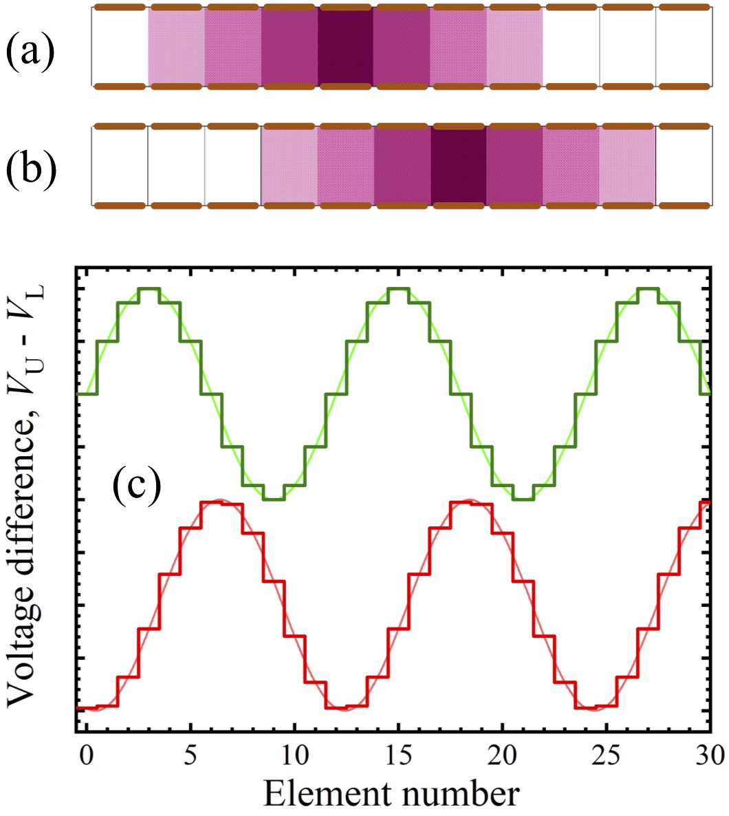
Figure 1: (a) Polarization-current antennas (PCAs) consist of a continuous series of elements made of a dielectric(white) sandwiched between pairs of electrodes (orange). The dielectric is polarized by applying a voltage difference $V_{\rm U}-V_{\rm L}$ between upper (U) and lower (L) electrodes; this is shown schematically for seven elements, the shading density representing the polarization strength. (b) The $V_{\rm U}-V_{\rm L}$ shown in (a) are applied to elements two further to the right, moving the polarized region. (c) The upper (green) trace shows $[V_{\rm U}-V_{\rm L}]_{j}=\sin[\omega(t-j\Delta t)]$ versus $j$, where $j$ labels the antenna element, $\omega$ is an angular frequency, $t$ is time and $\Delta t$ is a time increment, at $t=0$. The lower (red) trace (offset vertically for clarity) shows $[V_{\rm U}-V_{\rm L}]_{j}$ at $t=\frac{103}{180}\frac{2\pi}{\omega}$; the effect of the timing differences is to move the “voltage wave” (and the induced polarization) along. In practice, fringing effects round off the stepped voltages, leading to a smoother waveform (fine liines).

The paper is organized as follows. Section II gives a brief introduction to the type of polarization-current antenna used in this work, and how the polarization current within it is animated and accelerated; as the antennas may not be familiar to the general reader, additional detail is given in the Supplementary Information [SI] SI . Section III gives an account of the acceleration scheme for transmitting information to particular locations. Sections IV and V describe an experimental proof-of-concept of the effect carried out within a 6.5 m RF anechoic chamber. Finally, Section VI discusses the implications of this observation for communications and astronomy.

II Polarization-current antennas

In both dielectric-resonator antennas (DRAs) dielectric and polarization-current antennas (PCAs) dielectrics play a major role in the emission mechanisms. However, the two antenna types function in completely different ways; DRAs essentially use the dielectric to boost the effective size (and hence the efficiency) of a small antenna dielectric , whereas in PCAs, the dielectric hosts a moving, volume-distributed polarization current jap ; IEEE ; acS13 ; RadarPatent ; FeedMk1 ; FeedMk2 ; CryptoPatent . Consequently, PCAs usually consist of a continuous strip of a dielectric such as alumina with electrodes on either side [Fig. 1(a)]. Each electrode pair and the dielectric in between is referred to as an element; the elements are supplied independently with a voltage difference, $V=V_{\rm U}-V_{\rm L}$, where U and L refer to upper and lower electrodes. This produces polarization P in the dielectric. By changing $V_{\rm U}-V_{\rm L}$ on a series of elements, the polarized region is moved [Fig. 1(a), (b)]; owing to the time dependence imparted by movement, a polarization current, $\partial{\bf P}/\partial t$ is produced, and will, under the correct conditions, emit electromagnetic radiation jap ; IEEE ; acS13 ; RadarPatent ; FeedMk1 ; FeedMk2 ; CryptoPatent ; Ginzburg ; Schott .

PCAs are usually run by moving a continuous polarization current along the dielectric RadarPatent ; FeedMk1 ; FeedMk2 ; CryptoPatent .. This is accomplished by applying phase-shifted time-dependent signals to the elements SI . A simple example is given in Fig. 1(c), where the upper (green) trace shows $[V_{\rm U}-V_{\rm L}]_{j}=\sin[\omega(t-j\Delta t)]$ versus $j$, where $j$ labels the antenna element, $\omega$ is an angular frequency, $t$ is time and $\Delta t$ is a time increment, at $t=0$. The lower (red) trace shows $[V_{\rm U}-V_{\rm L}]_{j}$ at a later time; the effect of the time increments is to move the “voltage wave” and hence the induced polarization at a speed $v=a/\Delta t$, where $a$ is the distance between element centres. Acceleration is introduced by varying $\Delta t$ along the antenna’s length. Further details and typical emission properties are given in the SI SI .

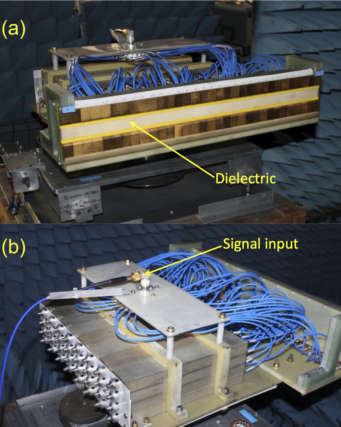
Figure 2: (a) Front view of the passive antenna used in the demonstration experiment mounted on its turntable in the anechoic chamber. It has 32 elements spanning a total length of 0.64 m. The label indicates the cream-colored dielectric (alumina) that hosts the volume-distributed moving polarization current responsible for the emission of radio waves from the antenna. (b) Rear view of the antenna showing the 32-way splitter feeding 32 independent ATM P1214 mechanical phase shifters. The dials for adjusting the phase are visible on the lower left of the picture. The signal input on the top of the 32-way splitter is labelled.

The practical antenna used in the experiments below is shown in Fig. 2(a); it has 32 elements spanning a total length of 0.64 m, and the dielectric is alumina $(\epsilon_{\rm r}\approx 10)$. The elements are fed via a 32-way splitter and 32 mechanical delay lines [Fig. 2(b)] which are adjusted to produce time differences $\Delta t$ [FeedMk2, ]. Note that in these antennas, the polarization current fills the entire dielectric; it is a continuously moving volume source of radiation that emits from an extended volume, rather than at a series of points or lines (as in a phased array). Despite the discrete nature of the electrodes, simulations of our antennas performed with off-the-shelf electromagnetic software packages such as Microwave Studio show that fringing fields of adjacent electrode pairs lead to a voltage phase that varies slightly under the electrode frank ; i.e., the phase is more smoothly varying along the length of the antenna than the discrete arrangement of electrodes suggests SI ; dissert . This is represented by the smoother curves in Fig. 1(c).

III Concept: acceleration and focusing

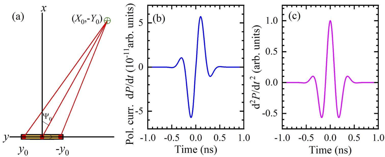
Figure 3: (a) Experimental concept. An element of polarization current (red) moves along the dielectric antenna (dark yellow shading) such that the component of its velocity in the direction of the target [green cross at $(X_{0},-Y_{0})$] is always $c$, the speed of light. The center of the antenna is at $(0,0)$. (b) Notional time dependence of the polarization current ${\rm d}P/{\rm d}t$ sent along the antenna. (c) Derivative of the curve shown in (b) with respect to time $t$. The “arbitrary units” in (c) are equivalent to those in (b), the large scaling occurring because of the fast time dependences.

We now consider an antenna containing a “wavepacket” of polarization current that has finite extent in both space and time; it moves on a linear trajectory and accelerates. Fig. 3(a) shows a plan view of the antenna’s dielectric of length $2y_{0}$ with its center at $(0,0,0)$ lying along the Cartesian $y-$axis. As in the experimental antennas FeedMk1 ; FeedMk2 ; CryptoPatent [Fig. 2(a)] the dielectric has rectangular cross-section; its depth $2x_{0}$ (extent in the $x$ direction) and height $2z_{0}$ (extent in the $z$ direction) are symmetrical about the $y$ axis; both $x_{0}$ and $z_{0}$ are $\ll y_{0}$.

A target is chosen in the $(x,y)$ plane at a distance $R_{0}$; the angle $\Psi_{0}$ “off boresight” describes the target’s azimuthal position. As everything of interest lies in the $(x,y)$ ($z=0$) plane, for convenience we drop the Cartesian $z$ coordinate for the time being. Thus, the target is at $(X_{0},-Y_{0})$, where

$$X_{0}=R_{0}\cos\Psi_{0}~{}~{}~{}~{}{\rm and}~{}~{}~{}~{}|Y_{0}|=R_{0}\sin\Psi_{0}.$$ (3)

Consider a point in the polarization current that is moving through the dielectic along the $y-$axis; the instantaneous distance $r$ between the point at $(0,y)$ and the target at $(X_{0},Y_{0})$ is given by

$$r^{2}=X_{0}^{2}+(Y_{0}+y)^{2}.$$ (4)

The point is made to move in such a way that the component of its velocity towards the target is always $c$, the speed of light in the surrounding medium (assumed to be vacuum), that is $({\rm d}r/{\rm d}t)=-c$, where $t$ is the time. Differentiating Eq. 4 with respect to $t$, inserting the above value for $({\rm d}r/{\rm d}t)$ and rearranging, we obtain the point’s velocity along $y$:

$$\frac{{\rm d}y}{{\rm d}t}=-c\frac{\left[X_{0}^{2}+(Y_{0}+y)^{2}\right]^{\frac{1}{2}}}{Y_{0}+y}.$$ (5)

Integrating Eq. 5, and assuming that the point commences its journey along the antenna at $y=y_{0}$ and time $t=0$, we obtain a relationship between the point’s position $y$ and time $t$:

$$t=\frac{1}{c}\left[(X_{0}^{2}+(Y_{0}+y_{0})^{2})^{\frac{1}{2}}-(X_{0}^{2}+(Y_{0}+y)^{2})^{\frac{1}{2}}\right].$$ (6)

We now consider a detector placed at a general point P with coordinates $(X,-Y)$ in the $(x,y)$ plane. The radiation emitted by the point as it travels along the antenna will reach P at a time $t_{\rm P}$ given by

$$t_{\rm p}=t+\frac{1}{c}(X^{2}+(Y+y)^{2})^{\frac{1}{2}}=\frac{1}{c}\left[(X_{0}^{2}+(Y_{0}+y_{0})^{2})^{\frac{1}{2}}-(X_{0}^{2}+(Y_{0}+y)^{2})^{\frac{1}{2}}+(X^{2}+(Y+y)^{2})^{\frac{1}{2}}\right].$$ (7)

It should be obvious that if, and only if, $X=X_{0}$ and $Y=Y_{0}$, then $t_{\rm P}=$ a constant. For all other choices of detector position, $t_{\rm P}$ is a function of $y$ and therefore of $t$.

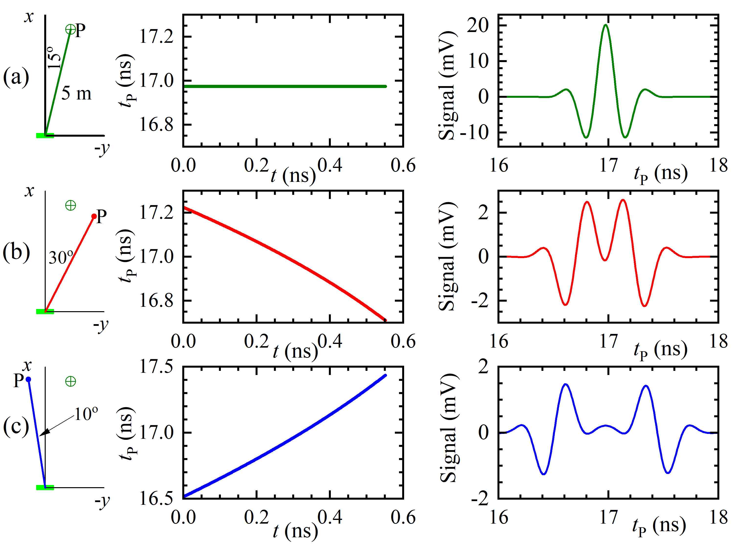
Figure 4: Each row shows the effect of moving the detector to positions P 5 m from the antenna center (light green). In each row, the left panel gives position P, the center shows the arrival time $t_{\rm P}$ of radiation emitted at time $t$ by a point accelerating along the antenna, and the right is the signal detected due to the polarization current of Fig. 3(b) being accelerated along the antenna. In all cases, the target (green cross) is 5 m from the antenna center at an angle of $15^{\circ}$ to the $x$ axis. Row (a): detector at target position. Row (b): detector placed on a line making an angle of $30^{\circ}$ with the $x$ axis. Row (c): detector placed $10^{\circ}$ to the other side of the $x$ axis.

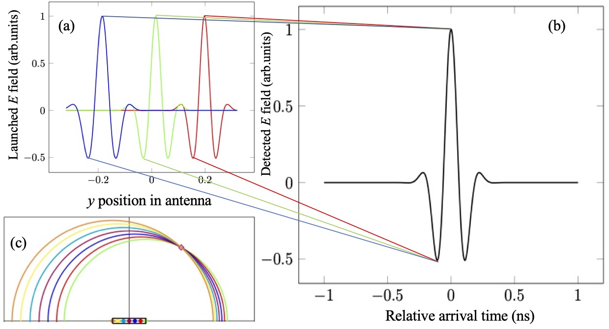
Figure 5: (a) Launched $E-$field [$\propto({\rm d}^{2}P/{\rm d}t^{2})$], corresponding to a polarization current similar to that in Fig. 3(b), at three different times (denoted by red, green and blue curves) during its transit along the antenna; note that the waveform “stretches out” due to the acceleration parameterized by Eqs. 3 and 6. (b) The corresponding detected $E-$field at the target point; colored lines linking (a) and (b) show schematically the principle that radiation from a particular point on the traveling waveform arrives at the same time at the target. This is because the acceleration compensates exactly for the different distances between source point and detection locations (see Eq. 7 et seq.). Hence, features in the launched $E$-field are reinforced in the correct time sequence in the detected signal. (c) The same principle is illustrated using Huyghens wavelets; colored dots in the antenna (dielectric outlined by black lines) represent the positions of a particular point on waveform (a) at different times during its transit of the antenna; semicircles of the same color show corresponding emittted Huyghens wavelets arriving at the focus point (orange diamond) simultaneously.

This situation is illustrated in the first two columns of Fig. 4. The intended target $(X_{0},-Y_{0})$ is at $R_{0}=5$ m from the antenna center and at $\Phi_{0}=15^{\circ}$ (Fig. 4, row (a), left column); if the detector P is placed exactly at this position, then $t_{\rm P}={\rm constant}$ (row (a), center column). The constant here is the transit time of light from $y=y_{0}$, the place at which the point source enters the antenna at $t=0$, to the target; subsequently the accelerated motion of the point source along the antenna exactly compensates for the changing point-to-target distance. If, on the other hand, the detector position P is not at $(X_{0},-Y_{0})$ [Fig. 4, rows (b) and (c)], then $t_{\rm P}$ is a function of $t$.

Next, rather than a single point, we consider the movement of the whole time-dependent polarization-current waveform along the antenna footnotexz . The imposed motion is such that each point within the waveform is accelerated as described above; i.e. as it traverses the antenna, such a point always has a velocity component $c$ in the direction of the target. Referring to the discussion of Eq. 7 above, all radiation emitted by this point as it moves along the antenna will arrive at the target at a time given by $t_{\rm P}=($time that point enters the antenna at $y=y_{0})+($transit time of light from $y=y_{0}$ to the target). Therefore, there is a one-to-one correspondence between the time at which each point on the moving waveform enters the antenna and the arrival time at the target of the radiation emitted by this particular point as it traverses the antenna.

To show how this affects the received radiation, we send the waveform shown in Fig. 3(b) along the antenna with the constraint that each point on the waveform obeys the acceleration scheme described by Eqs. 3 and 6; as before $\Phi_{0}=15^{\circ}$ and $R_{0}=5.0$ m. The resulting signals (proportional to the $E-$field) for the detector positions given in the first column of Fig. 4 are shown in the third column of the same figure; the SI describes how such calculations are carried out SI ; dissert . At the target angle and distance [(Fig. 4, row (a)], the detected signal reproduces the shape of the time derivative of the polarization-current waveform [Fig. 3(c)] exactly. Away from the target position [Fig. 4, rows (b) and (c)], the detected signal is much smaller and has altered frequency content and shape.

First, why is the time-derivative of the polarization current reproduced? The calculations in the SI show that SI ; dissert the magnetic vector potential A resulting from each volume element of the antenna is proportional to the polarization current within that element (SI, Eq. 8 [SI, ]). The corresponding $E-$field is proportional to the derivative of ${\bf A}$ with respect to time Bleaney . Therefore, it is the electric field launched from the antenna that is reproduced at, and only at, the target point.

The idea is illustrated in more detail in Fig. 5; (a) shows the launched $E-$field [$\propto({\rm d}^{2}P/{\rm d}t^{2})$] at three different times indicated by different colors during its transit through the antenna. Figure 5(b) shows the corresponding detected $E-$field at the target point. The colored lines linking the curves in Figs. 5(a) and (b) illustrate the principle that radiation from a particular point on the traveling waveform always arrives at the same time at the target. Thus, features in the launched $E$-field are reinforced at the target in the correct time sequence. In other words, the time dependence of the emission of the whole waveform is reproduced at the target [compare Figs 3(c) and 4(a)] whereas elsewhere, it is scrambled [Figs. 4(b), (c)].

Fig. 5(c) illustrates the same principle using Huyghens wavelets. The colored dots represent the positions of a particular point on the polarization-current waveform at different times during its transit of the antenna; semicircles of the same color represent the corresponding emitted Huyghens wavelets, arriving at the target (orange diamond) simultaneously. At other locations, the Huyghens wavelets arrive at different times, so that the signal becomes scrambled.

For the experimental demonstration below, we need to describe a polarization-current waveform the possesses the required motion for the above focusing effects. To do this, we write footnotexz

$$\frac{\partial{\bf P}}{\partial t}={\bf f}(y,t)={\bf f}[t-p(y)],$$ (8)

where f is a vector function of time $t$ and the function $p(y)$. Constant phase points are represented by $t-p(y)={\rm constant}$; differentiating this with respect to $t$ results in

$$1=\frac{{\rm d}p}{{\rm d}t}=\frac{{\rm d}p}{{\rm d}y}\frac{{\rm d}y}{{\rm d}t}$$ (9)

Substituting from Eq. 5 and integrating, we obtain

$$p(y)=-\frac{\left[X_{0}^{2}+(Y_{0}+y)^{2}\right]^{\frac{1}{2}}}{c}.$$ (10)

Eqs. 8 and 10 describe the required extended polarization current waveform, all of the points within which approach the target at a speed of $c$.

Finally, note that we have only treated a time-domain focus in the $(x,y)$ plane. In fact the criterion for focusing - that points in the polarization-current distribution approach the observer/detector at the speed of light along their entire path though the antenna - is fulfilled on a semicircle of points around the antenna [our antennas are designed not to emit from their rear surfaces FeedMk2 ] that extends in the $y$ and $z$ directions, with a radius $(y^{2}+z^{2})^{1/2}=Y_{0}$. However, in a proof-of-concept demonstration experiment, moving the observer/detector away from $z=0$ complicates matters, as the radiation’s $E$-field is no longer vertically polarized; there is an additional component polarized parallel to $y$ [this may be deduced from the calculations in the SI SI ; for more details see Chapter 6 of Ref. dissert, ]. In the next implementation of this concept, the single antenna discussed in the present paper is replaced by an array of linear antennas configured to allow full three-dimensional $(x,y,z)$ control of the information focus point, along with minimization of the parasitic $y$ polarization of the $E$-field nichols .

IV Experimental demonstration

The antenna shown in Fig. 2 is used for the experimental demonstration. It is mounted on a powered turntable (vertical rotation axis) with an azimuthal angular precision of $\pm 0.1^{\circ}$. A Schwarzbeck-Mess calibrated dipole at the same vertical height is used to receive the vertically polarized transmitted radiation; this is mounted on a TDK plastic tripod on rails that allows it to be moved to different distances without changing the height or angular alignment of the equipment. The entire system is in a $5.8\times 3.6\times 3.6$ m³ metal anechoic chamber completely lined with ETS-Lindgren EHP-12PCL pyramidal absorber tiles.

Signals received by the dipole are sent either to a Hewlett-Packard HP8595E spectrum analyzer to monitor power at a chosen frequency, or to a Mini-Circuits TVA-82-213A broadband amplifier that allows the time-dependent voltage to be viewed and/or digitized using a Tektronix TDS7404 digital oscilloscope. Care is taken to ensure that the cables used are shielded from the radiation within the anechoic chamber and that secondary-path signals are $\sim 60$ dB less than direct radiation from antenna to dipole.

The description in Section III is framed in terms of a traveling wavepacket. However, detecting a single pulse, especially if it contains a spread of frequencies, presents technical difficulties in a facility where only low power levels are permitted. Instead, we choose to transmit and detect what is in effect a train of wavepackets. This forms a continuous broadband signal with a distinctive shape, based on a mixture of harmonics of 0.90 GHz and synthesized by mixing outputs from phase-locked TTi TGR6000 and Agilent N9318 function generators.

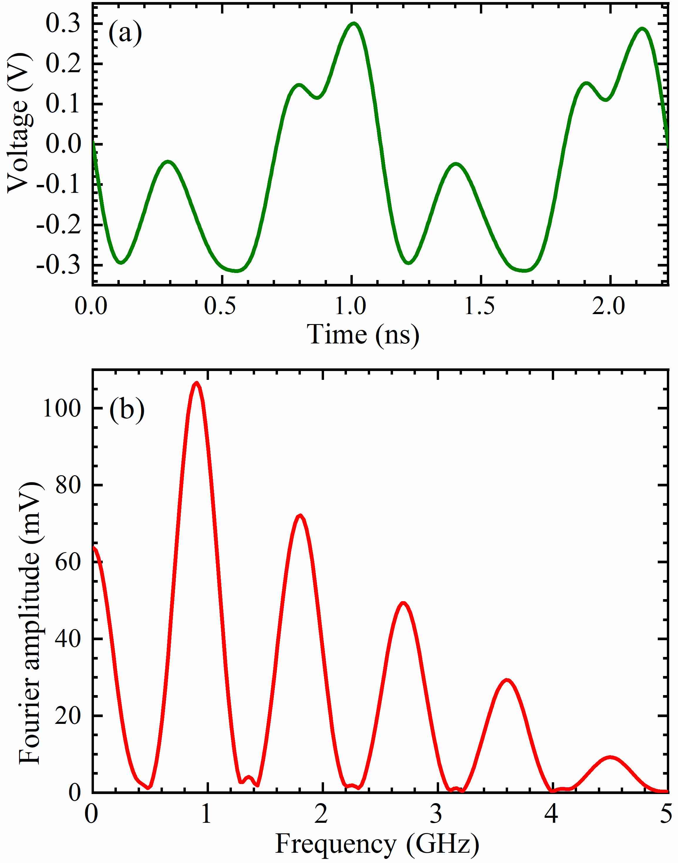
Figure 6: (a) The voltage measured by placing the dipole receiver 10 mm in front of the 16th antenna element as a function of time; in effect, this is the desired transmitted signal. (b) Fourier transform of the waveform in (a). Note the distinctive “triangular” pattern of harmonics of 0.9 GHz.

The synthesized signal is sent to a Mini-Circuits TVA-82-213A amplifier, the output of which drives a 32-way splitter feeding 32 independent ATM P1214 mechanical phase shifters [Fig. 2(b)]. The latter are used to set the time-delays of the signals sent to each antenna element, reproducing the above acceleration scheme. To keep the “information focus” well within the anechoic chamber, $X_{0}=3.03$ m and $Y_{0}=0.64$ m are chosen, yielding target distance $R_{0}=3.09$ m and azimuthal angle $\Phi_{0}=11.9^{\circ}$.

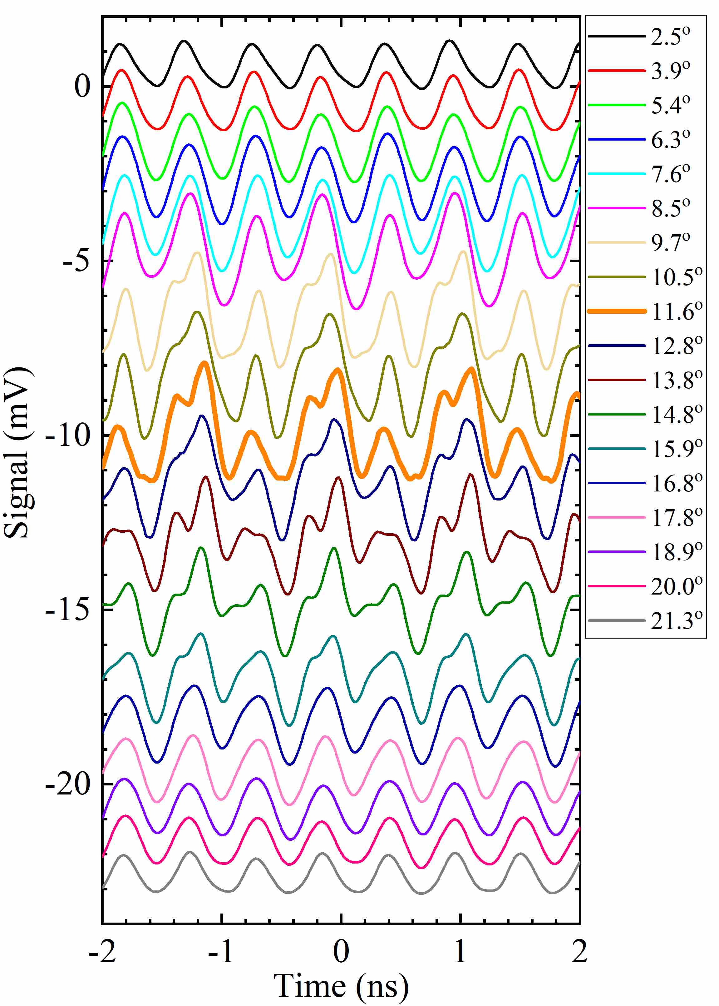
Figure 7: Time dependence of the signal received by the detector dipole for an antenna-to-detector distance of 3.0 m and for the azimuthal angles shown in the key. The shape of the transmitted waveform (Figure 6(b)) is only reproduced close to the “target” angle of $11.6^{\circ}$ (orange trace). Experimental traces are offset vertically for clarity.

The time-dependence of the broadcast waveform is recorded by placing the receiver dipole 10 mm in front of the 16th element of the antenna and observing the signal on the oscilloscope. As long as the shortest emitted wavelength is much larger than distance from the dielectric to the detector, the calculations described in the SI SI can be used to show that the $E$-field thus detected by the dipole is, to a good approximation, $\propto\partial^{2}{\bf P}/\partial t^{2}$, where ${\bf P}$ is the polarization passing the point in the dielectric closest to the detector antenna. Hence, an analogue of Fig. 3(c) for the experimental wavetrain is captured; moreover, any frequency-dependent artefacts are the same in the measurements of the broadcast and received signals, making a comparison analogous to that between Fig. 3(b) and the third column of Fig. 4 simpler.

The waveform used for the experiments is selected by adjusting the outputs of the two signal generators and is shown in Fig. 6(a). It is chosen because (i) it has a distinctive time-dependent shape (e.g. the double peak followed by two differing minima, one relatively broad) and (ii) an easily recognized “triangular” Fourier spectrum [Fig. 6(b)]. These traits aid in the rapid location of ranges of distance and azimuthal angle over which the broadcast signal was reproduced.

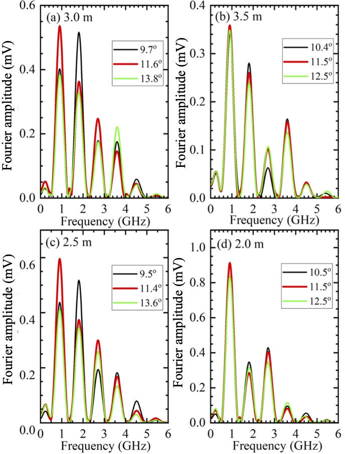
Figure 8: Fourier transforms of the detector signal for azimuthal angles (shown in key) on either side of (green and black) and close to or at the target angle of $11.6^{\circ}$ (red) and at different antenna to detector distances: (a) 3.0 m, (b) 3.5 m, (c) 2.5 m and (d) 2.0 m.

V Results

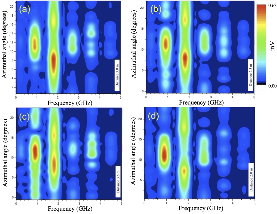
Figure 9: Fourier transforms of the detector signal plotted as contour plots versus frequency and azimuthal angle for different antenna to detector distances: (a) 3.0 m, (b) 2.5 m, (c) 3.5 m and (d) 2.0 m.

Preliminary surveys are carried out by sweeping the transmitter azimuthal angle at closely spaced distances around the expected $R_{0}$ whilst carefully observing the received signal on the oscilloscope or spectrum analyzer. Slight phase-setting errors result in actual target coordinates $R_{0}\approx 3.00$ m and $\Phi_{0}\approx 11.6^{\circ}$ (c.f. planned values of $3.09$ m and $11.9^{\circ}$).

Once this “focus” is established, the transmitter-to-receiver distance is fixed at 3.0 m and the oscilloscope trace of the received signal recorded for several fixed azimuthal angles spaced by $\approx 1^{\circ}$. The results of this procedure are shown in Fig. 7. On comparing with Fig. 6(a), it is clear that the broadcast signal (double peak, narrower then wider minimum) is only reproduced faithfully at an azimuthal angle of $11.6^{\circ}$ (orange, thicker curve). The time-dependent signals for angles $12.8^{\circ}$ and $10.5^{\circ}$ show distinct differences from the broadcast waveform; one only has to move a few more degrees away from $\Psi_{0}$ and any resemblance to the broadcast signal is lost.

This picture is confirmed by Fourier transforms of the oscilloscope data [Fig. 8(a)]. At an angle of $11.6^{\circ}$ (red trace), the expected “triangular” Fourier spectrum [c.f. Fig. 6(b)] is produced. On moving $\approx\pm 2^{\circ}$ away, the relative amplitudes of the harmonics of 0.9 GHz change quite dramatically, showing that the frequency content present in the broadcast signal is being scrambled.

Measurements are then repeated at fixed transmitter-to-receiver distances either side of the target distance of $R_{0}=3.0$ m [Fig. 8(b)-(d)]. Even azimuthal angles close to the target value (red traces) fail to yield the broadcast “triangular” Fourier spectrum [compare with Figs. 8(a), 6(b)], showing that the frequency content of the original broadcast signal is only reproduced when the distance and the azimuthal angle are close to the target values. Fourier transforms taken over wider angular ranges are given in the contour plots of Fig. 9, showing that the “triangular” Fourier spectrum is not recovered as one moves farther from the target angle.

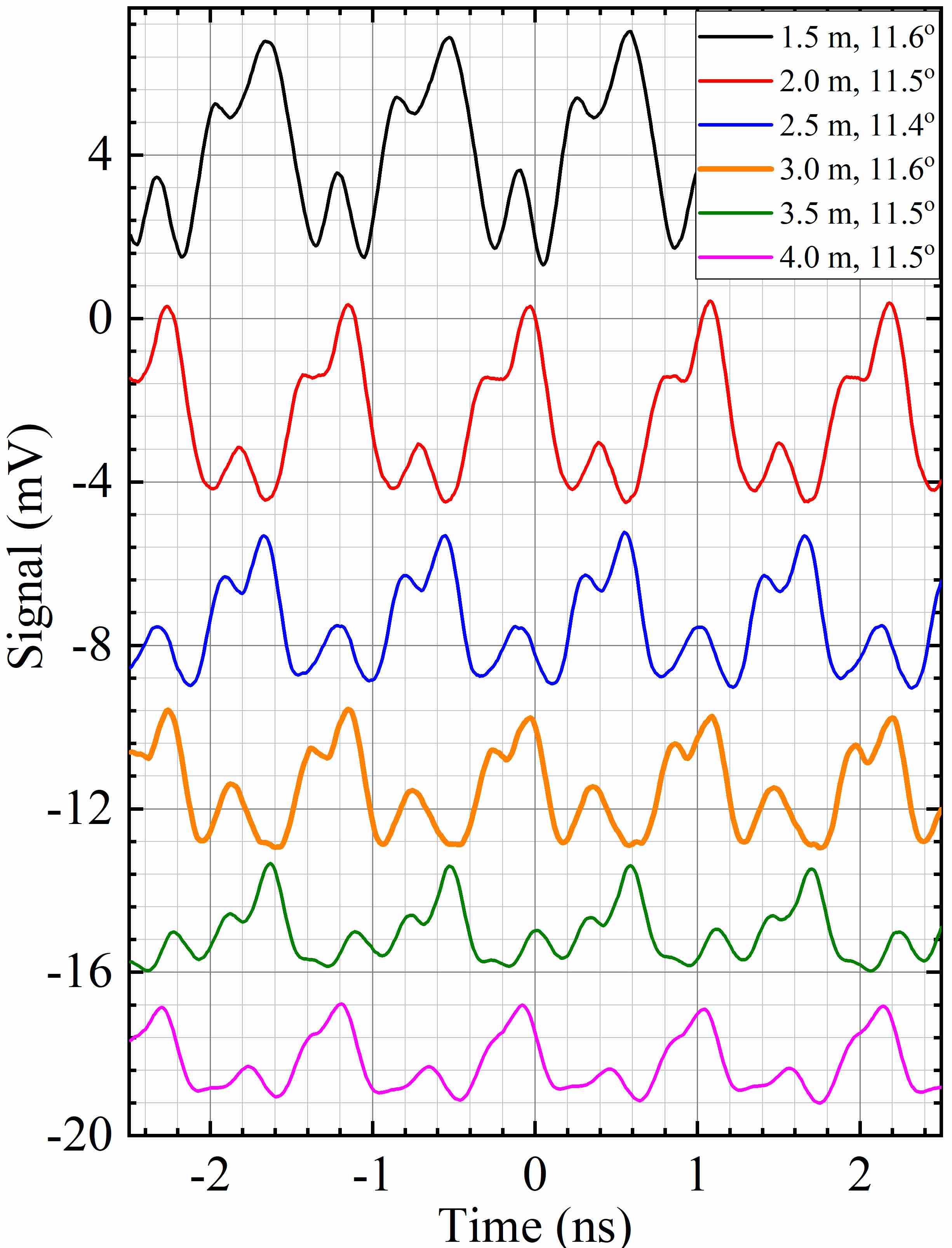
Figure 10: Time depndence of the signal received by the detector dipole for azimuthal angle close to $\Phi_{0}=11.6^{\circ}$ and for different antenna-to-detector distances shown in the key. The shape of the transmitted waveform (Fig. 6(b)) is only reproduced close to the “target” $R_{0}=3.0$ m (orange trace).

Fig. 10 shows the effect on the time dependence of the received signal caused by keeping the azimuthal angle close to $\Phi_{0}=11.6^{\circ}$ and varying the transmitter-to-receiver distance. Comparing Fig. 10 with Fig. 6(a), it is clear that the broadcast signal’s time dependence (double peak, narrower and then wider minimum) is only reproduced faithfully at distances close to the target value of $3.0$ m (orange, thicker curve).

VI Discussion

The data displayed in Figs. 6 to 10 show that a continuous, linear, dielectric antenna in which a superluminal polarization-current distribution accelerates can be used to transmit a broadband signal that is reproduced in a comprehensible form at a chosen target distance and angle; as noted in the final paragraph of Section III, effectively this signal is distributed onto a half circle dissert in ’the current implementation of the experiment nichols . The requirement for this exact correspondence between broadcast and received signals is that each point in the polarization-current distribution approaches the observer/detector at the speed of light at all times during its transit along the antenna. This results in all of the radiation emitted from this point as it traverses the antenna reaching the observer/detector at the same time [Fig. 4(a)]. For other observer/detector positions, the time dependence of the signal is scrambled, due to the non-trivial relationship between emission time and reception time [Figs, 4(b), (c)].

The primary rôle of the current paper is to introduce the above effect and to demonstrate it experimentally. However, it is interesting to suggest how a PCA might be employed to transmit signals that contain information. Fig. 11 depicts a simulation of a simple version of such a concept. The inset shows the time dependence of a wavepacket of launched $E-$field that could function as a single “bit”. Like the waveforms employed in Figs. 3 and 4, it consists of the convolution of a Gaussian and a cosine. The main part of the Figure shows a calculation (using the techniques detailed in the SI SI ) of the received signal due to the broadcast of two of these “bits”, spaced in time by three periods of the cosine function. For ease of comparison, the antenna accelaration scheme [i.e., target angle $(15^{\circ})$ and distance (5.0 m)] is the same as that employed in Fig. 4. At the target angle of $15^{\circ}$, the two “bits” can be distinguished clearly (labelled 1 and 2 in Fig. 11); as one moves the receiver away from the target angle by as little as $5^{\circ}$, the received signal falls off in amplitude and the individual “bits” become almost impossible to distinguish. This example shows only two “bits”; however, a longer string of similar “ones” and “zeros” would also suffer an analogous smearing as one moved away from the target position.

In this context, note that the depth of focus (i.e., the range of distance and angle over which the signal is comprehensible) depends strongly on the form and frequency content of the broadcast signal. For example, the waveform used in the experiment, which encompasses frequencies from 0.9 to 4.5 GHz [see Fig. 6], results in a received signal that distorts relatively quickly as the detector moves out beyond the target distance of $R_{0}=3.0$ m at the target angle [Fig. 10]. By contrast, a relatively narrow-band broadcast signal [e.g., Fig. 3] will be recognizable at the target angle over a wider range of detector distances dissert . A full discussion of the criteria for the tightness of “information focusing” demands detailed analysis of many different broadband signal types and goes beyond the scope of the current work; instead, it forms the basis of a subsequent paper geology .

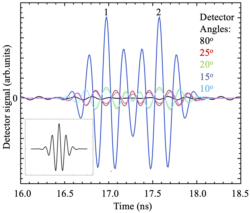
Figure 11: Simulation of a notional method for transmitting information only to a target point. The inset shows a “bit” (consisting of a Gaussian convoluted with a cosine) as it would appear in the time-dependence of the broadcast $E-$field [compare with Fig. 3(c)]. The main figure shows a calculation of the detected signal at a range of 5 m. This results from time-spacing two of these “bits” by three periods of the cosine function and then subjecting them to the same acceleration scheme that is used to produce Fig. 4. At the target angle of $15^{\circ}$ (dark blue), the “bits” (labelled 1 and 2) may be easily resolved. However, as soon as the detector is moved to other angles (labelled by the colors in the key), the received signal is much weaker and the “bits” become virtually impossible to distinguish.

This technique represents a contrast to conventional radio transmission methods. In many instances of the latter, signals are broadcast with little or no directivity, selectivity of reception being achieved through the use of one or more narrow frequency bands Balanis ; Godara ; adamy ; ken . In place of this, the current paper uses a spread of frequencies to transmit information to a particular location; the signal is weaker and has a scrambled time dependence elsewhere [Fig. 4]. A possible application may be in proposed 5G neighbourhood networks, where a single active antenna will sequentially spray bursts of information into a selection of target buildings around it 5G1 ; 5G2 ; ensuring that neighbours cannot easily understand what you are transmitting and receiving will be an important component.

The work in this paper may also be relevant to pulsars, rotating neutron stars that possess very large, off-axis magnetic fields and plasma atmospheres pulse1 ; pulse2 . Pulsar periods of rotation $2\pi/\eta$ range from 1.5 ms to 8.5 s; a back-of-the-envelope calculation shows that at surprisingly small distances (85 km for the 1.5 ms pulsar; 40,000 km for the 8.5 s one) from the rotation axis, the pulsar’s magnetic field will be travelling through its plasma atmosphere faster than the speed of light. Hydrodynamical models of pulsars hyd1 ; hyd2 ; hyd3 show the following: (i) electromagnetic disturbances (identifiable as polarization currents) exist outside the light cylinder, the orthogonal distance from the rotation axis $r_{\rm L}$ at which $\eta r_{\rm L}=c$; (ii) these disturbances rotate at the same angular velocity as the neutron star’s magnetic field (a requirement of Maxwell’s Equations), and so travel superluminally at radii outside the light cylinder; and (iii) the most intense disturbances are compact, in that they occupy a small fraction of the pulsar’s atmosphere.

For such a compact source, traveling on a circular path at faster-than-light speeds, a derivation given in the SI SI shows that a plot of observation/detection time $t_{\rm P}$ versus emission time $t$ exhibits “plateaux” [see Fig. 18 of the SI] at, and only at, a special polar angle determined by the source’s tangential speed. Apart from a single point at their center where ${\rm d}t_{\rm P}/{\rm d}t=0$, these “plateaux” are not, in fact, flat dissert . However, there is a reasonable region of $t$ over which ${\rm d}t_{\rm P}/{\rm d}t\ll 1$, so that a situation similar to that in Fig. 4(a) may be possible.

Pulsars can potentially emit electromagnetic radiation via many mechanisms pulse1 ; pulse2 , including thermal emission and other processes in their hot, plasma atmospheres, and dipole radiation from the rotating magnetic field of the neutron-star core; why then, might the pulsed radiation detected on Earth be dominated by the small volume of superluminal polarization current? The similarity of the “plateaux” in Fig. 18 of the SI to Fig. 4(a) provides an important clue. At the focus polar angle and over a short window of $t_{\rm P}$, the frequency content of all of the emission processes occurring within the rotating polarization-current element will reproduce exactly, and result in a detected signal with greatly enhanced amplitude; the result is similar to coherent emission Brooker , but via a completely different mechanism. At all other observation angles and observation times, radiation from the emission processes will superpose incoherently [c.f. Figs. 4(b), (c)], leading to a greatly reduced amplitude, and scrambled frequency content. The sharp focusing in the time domain at the focus polar angle is likely to allow the radiation produced by the superluminal (outside the light cylinder) mechanisms to dominate the pulses. Note that this explanation of the brightness of pulsar pulses does not depend on the incorrect proposal HADemolish of non-spherical decay advocated by Ardavan HA1 ; HA2 ; HA3 .

VII Summary

The experiments in this paper show that a continuous, linear, dielectric antenna in which a superluminal polarization-current distribution accelerates can be used to transmit a broadband signal that is reproduced in a comprehensible form at a chosen target distance and angle. This is due to all of the radiation emitted from this point as it traverses the antenna reaching the observer/detector at the same time. For other observer/detector positions, the time dependence of the signal is scrambled, due to the non-trivial relationship between emission (retarded) time and reception time . The results may be relevant to 5G neighbourhood networks and pulsar astronomy.

Appendix: Supplementary Information

VIII Demonstration of speed control of polarization currents

VIII.1 Superluminal speeds

As an illustration, Sec. 2 of the main paper describes the simplest method to produce a polarization current moving at a constant speed jap ; IEEE ; FeedMk1 ; FeedMk2 ; CryptoPatent ; the $j$th ($j=1$, 2, 3….) element of the antenna is supplied with time-dependent voltage differences

$$V_{j}=[V_{\rm U}-V_{\rm L}]_{j}=V_{0}\cos[\omega(t-j\Delta t)],$$ (11)

where the symbols are defined in the main paper. The voltages $V_{j}$ are usually $\leq 1$ V; under these, and much higher voltages, alumina behaves as a linear dielectric, so that the polarization P in the $j$th element will be proportional to the electric field Jackson ; Balanis ; Bleaney generated by $V_{j}$. The polarization current that emits the radiation from the antenna is thus “dragged along” by the time-dependent voltages applied to the elements at a speed $v=a/\Delta t$, where $a$ is the separation of the centers of adjacent elements.

In the early years of the 20^th Century, both Sommerfeldt Sommerfeldt and Schott Schott showed that emission of electromagnetic radiation from such a moving source can only occur when $v>c$, the speed of light in vacuo. Schott demonstrated Schott that the Huygens wavelets from each point in the moving polarization current form a conical envelope with aperture $\sin^{-1}(c/v)$ [Fig. 12(a)]. Translating this to an extended, moving polarization current that fills the entire antenna, this results in emitted power that should peak at an azimuthal angle

$$\phi=\sin^{-1}\left(c/v\right).$$ (12)

To demonstrate this effect, we use data from the antenna FeedMk1 shown in Fig. 13(a). Like the antenna in the main paper, it comprises 32 elements and employs alumina $(\epsilon_{\rm r}\approx 10)$ as a dielectric, but it has a smaller element spacing of $a=10.87$ mm. The detected power is monitored using a Schwarzbeck Mess calibrated dipole whilst the antenna is rotated on a turntable to vary the azimuthal angle $\phi$.

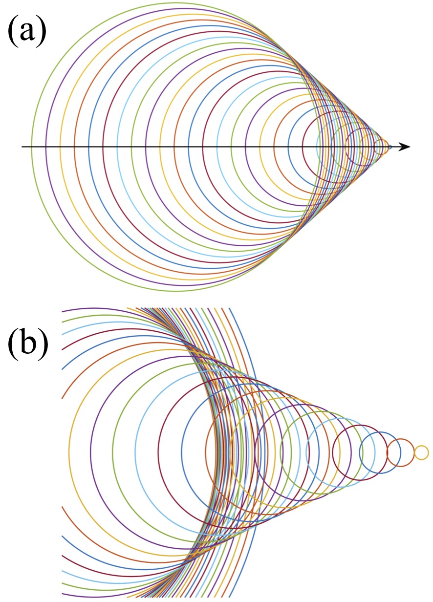
Figure 12: (a) Huygens wavelets emitted by a small source of electromagnetic radiation traveling along a rectilinear path with constant superluminal speed, $v/c=1.5$. Since the source travels faster than the waves it emits, it leads the advancing wave-front; the envelope of the Huygens wavelets is a vacuum Čerenkov cone with half-angle $\sin^{-1}(c/v)$. (b) Huygens wavelets emitted by a small source moving along a straight line with constant acceleration. Having broken the “light barrier”, the source leaves a Čerenkov envelope in its wake that has a slightly concave lateral surface. Note the clustering of many Huygens wavelets to either side (i.e., in a ring around the source’s path); this represents the arrival, in a relatively short period of observation time, of radiation emitted over an extended length of the source’s path. In the main paper, we optimize the acceleration so that the Huygens wavelets emitted over the entire path of a point source arrive simultaneously at a chosen “target”. [After Ref. dissert, , adapted from Schott Schott .]

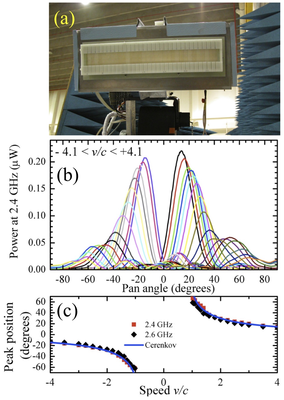
Figure 13: (a) The antenna used in the vacuum Čerenkov demonstration placed on a stepper-motor-driven pan/tilt mount. (b) Power received from the antenna run at several different constant speeds $v$, ranging from $-4.1c$ to $-1.1c$ and $+1.1c$ to $+4.1c$, versus azimuthal (pan) angle. The emitted frequency is $\frac{\omega}{2\pi}=2.4$ GHz and the detector is 5.36 m from the antenna in an anechoic chamber. (c) Peak power angle versus polarization-current speed $v$ with $\frac{\omega}{2\pi}=2.4$ GHz and $\frac{\omega}{2\pi}=2.6$ GHz (points); the curve is the prediction for the vacuum Čerenkov effect [Eq. 12].

Fig. 13(b) shows detected power (in $\mu$W) versus $\phi$ for the antenna running at a series of constant speeds $v$, set by varying $\Delta t$ in Eq. 11. When plotted in these linear power units, the azimuthal dependence is clearly dominated by a single, large peak, the angle of which depends on $v$. Fig. 13(c) shows that the azimuthal angle $\phi$ at which peak power occurs varies with $v$ as expected for the vacuum Čerenkov effect Schott [Eq. 12].

VIII.2 Subluminal speeds

When polarization-current antennas are run at constant speeds $v/c<1$, the power detected oscillates as a function of azimuthal angle. Fig. 14(a) gives an example of this behavior; to obtain these data, the antenna shown in Fig. 13(a) was run at $v/c=0.5$. In addition to the oscillations, the peak power is some $15-20$ dB lower than for speeds $v/c\approx 2-4$.

The power oscillations in Fig. 14(a) are similar to those from a two-slit diffraction experiment in which the light from one slit is $(2\aleph+1)\pi$ out of phase with that from the other, where $\aleph$ is an integer. In the far field, such a two-slit experiment would give minima that occur when Brooker

$$b\sin\phi=l\lambda,$$ (13)

where $b$ is the spacing of the slits, $l$ is an integer and $\lambda$ is the wavelength. Hence, a plot of $\sin\phi$ versus $l$ should be a straight line, with gradient $\lambda/b$. Fig. 14 shows that the minima indeed obey this relationship. The reasons for this will be discussed in more detail below.

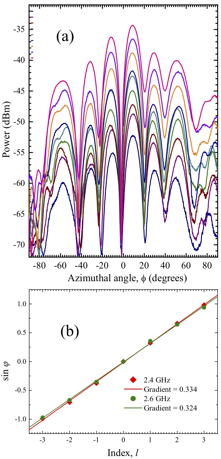
Figure 14: (a) Received power versus azimuthal angle $\phi$ for antenna-to-detector distances 0.95, 1.4, 1.8, 2.3, 3.2, 4.1, 5.2, 5.4 and $8.6$ m, and subluminal source speed $v/c=0.5$; the antenna used is that in Fig. 13(a) and data are shown for $\omega/2\pi=2.6$ GHz. (b) A plot of $\sin\phi$ versus index $l$, where $\phi$ denotes the angle at which a minimum in power occurs, for a distance of 8.6 m [see (a)]. Data are points, and the lines are straight-line fits, giving gradients of 0.33 and 0.32 for $\omega/2\pi=2.4~{}$GHz and 2.6 GHz points respectively.

IX Feeds to antenna elements

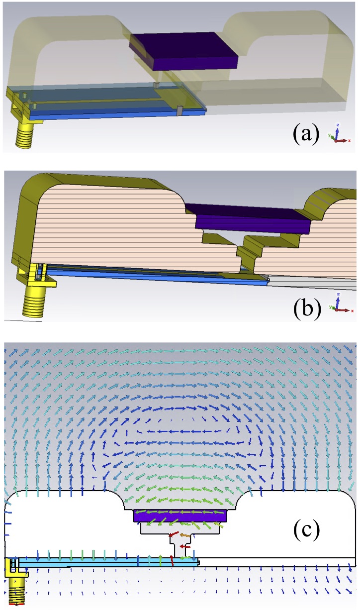
Figure 15: (a, b) Two views of an individual element of the antenna shown in Fig. 2 of the main paper. The RF signal is fed from an SMA connector and coupled to a micro-stripline (gold on blue). The final rectangular patch underneath the cut-out opening and the shape of the stepped opening above transform the field pattern into a linearly polarized electric field across the alumina dielectric (purple) between the electrodes. The whole upper part of the element is made up from two pieces of copper-plated G10. (c) The fields (arrows) from the polarization current in the element radiate out of the top surface only. Transverse components of the fields are suppressed by the proximity of the neighboring antenna elements.

An important ingredient of the design of polarization-current antennas is the way in which radiofrequency (RF) signals are transformed from cylindrical propagating modes in $50~{}\Omega$ coaxial cable to a linear electric field applied by the electrodes to the dielectric FeedMk1 ; FeedMk2 ; dissert . Figs. 15(a,b) show how this is achieved in the antenna depicted in Fig. 2 of the main paper. Most of the antenna element is made from G10 composite, with the upper surface plated with copper. The radiofrequency signal is fed from an SMA connector ($50~{}\Omega$) and coupled to an impedance-matched micro-stripline built on standard circuit board. The final transformation into the desired, linear field pattern to be applied to the dielectric is achieved by a rectangular patch underneath the cut-out opening and the shape of the stepped opening above.

Note that the individual elements cannot be designed, modelled or tested on their own; isolated, they do not have the desired characteristics for the function of the antenna. Instead, their performance depends on the presence of neighboring elements. Fig. 15(c) shows how the fields from the polarization current in the element radiate out of the top surface only; the transverse components of the fields are suppressed by the proximity of the adjacent antenna elements. The design of the elements also suppresses radiation out of the back of the antenna, increasing the directivity.

In practice, the antenna elements can be built individually and then combined into different configurations optimized for particular applications dissert . Alternatively, all of the elements for an antenna can be fashioned on a single monolithic substrate (machined from a G10 block by a CNC mill) for strength and rigidity.

X Calculation of emitted radiation

X.1 Basic principles

Simulated antenna emissions are used to illustrate the principles of the experiment in the main body of the paper. Therefore, a brief explanation of the simulations and a validation via comparison with experimental data taken using the antenna shown in Fig. 13(a) are now given.

Despite the discrete nature of the electrodes, simulations of our antennas performed with off-the-shelf electromagnetic software packages show that fringing fields of adjacent electrode pairs lead to a voltage phase that varies under the electrode frank ; i.e., the phase varies much more smoothly than the discrete electrodes suggest. Therefore we represent the position dependence of the voltage applied across the dielectric as a continuous function, giving two examples below.

(i) For a constant speed (c.f. Eq. 11) we consider a traveling, oscillatory voltage applied symmetrically across the dielectric in the vertical $z$ direction, $V=V_{0}{\rm e}^{{\rm i}(\omega t-ky)}$. Here $y$ is the distance along the antenna’s long axis and $V_{0}$ and $k$ are constants. Let the dielectric extend from $z=-z_{0}$ to $z=+z_{0}$ in the vertical direction; assuming that it is uniform, the potential at a general position $(y,z)$ in the dielectric is

$$V(y,z,t)=V_{0}\frac{z}{2z_{0}}{\rm e}^{{\rm i}(\omega t-ky)}.$$ (14)

(ii) For the wavepacket shown in Fig. 2, main paper, the voltage is given by $V_{0}{\rm e}^{{\rm i}\omega[t-p(y)]}{\rm e}^{-\alpha^{2}[t-p(y)]^{2}},$ where $\alpha$ is a constant. This consists of a Gaussian convoluted with a travelling wave; both have the $(y,t)$ dependence [given by $p(y)$] required for the motion described in the main paper. Under the same assumptions as (i), the potential at $(y,z)$ in the dielectric is

$$V(y,z,t)=V_{0}\frac{z}{2z_{0}}{\rm e}^{{\rm i}\omega[t-p(y)]}{\rm e}^{-\alpha^{2}[t-p(y)]^{2}}.$$ (15)

For either equation, the polarization P is obtained Bleaney by

$${\bf P}=\epsilon_{0}(\epsilon_{r}-1){\bf E}=\epsilon_{0}(\epsilon_{r}-1)[-\nabla V(y,z,t)].$$ (16)

Differentiating with respect to time, we obtain a polarization-current density Bleaney

$${\bf J}(y,z,t)=\frac{\partial{\bf P}}{\partial t}$$ (17)

In evaluating the emitted radiation, we consider only the contribution of ${\bf J}$ in the dielectric; there is a negligible conduction current, and we neglect the free charges that exist only at the interface between the dielectric and the electrodes. In this situation, the following equation Balanis ; Bleaney ; Jefimenko can be used to evaluate the magnetic vector potential ${\bf A}$ at the observer/detector’s remote location ${\bf r}_{\rm P}=(X,Y,Z)$ and at the observation time $t_{\rm P}$:

$${\bf A}({\bf r}_{\rm P},t_{\rm P})=\frac{\mu_{0}}{4\pi}\int^{z_{0}}_{-z_{0}}\int^{y_{0}}_{-y_{0}}\int^{x_{0}}_{-x_{0}}\frac{{\bf J}({\bf r},t)}{|{\bf r}_{\rm P}-{\bf r}|}{\rm d}x{\rm d}y{\rm d}z$$ (18)

Here, ${\bf r}=(x,y,z)$ is a coordinate within the dielectric. The integration is carried out over the volume of the dielectric; as in the main paper, its length is $2y_{0}$ and its thickness in the $x$ direction is $2x_{0}$. The retarded time $t$ varies for different locations r within the dielectric:

$$t=t_{\rm P}-\frac{|{\bf r}_{\rm P}-{\bf r}|}{c}.$$ (19)

Here $c$ again denotes the speed of electromagnetic waves in the medium (assumed to be uniform) between the source and the observer.

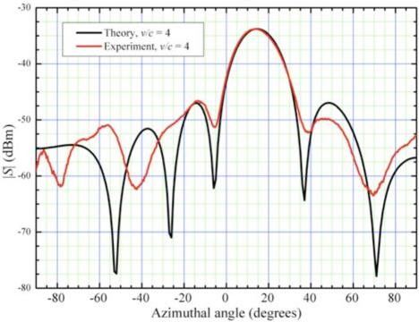
Figure 16: Modulus of Poynting vector $|S|$ [Eq. 22] versus azimuthal angle $\phi$ (black) predicted by the calculations. The antenna dimensions are based on the example shown in Fig. 13(a). The frequency is $\omega/2\pi=2.4$ GHz, $v/c=4$ and the antenna to detector distance is 5 m. Experimental data for the same antenna, measured at the same distance (5 m) in an anechoic chamber are shown in red. After correction for the gain of the detector dipole and losses in its cables, there is a reasonable quantitative match between experiment and calculation.

The corresponding radiation fields are derived from differentiating ${\bf A}$ with respect to the observer’s coordinates $(X,Y,Z,t_{\rm P})$. The electric field is given by Jackson ; Bleaney

$${\bf E}(X,Y,Z,t_{\rm P})=\frac{\partial{\bf A}(X,Y,Z,t_{\rm P})}{\partial t_{\rm P}},$$ (20)

and since the magnetic flux is always solenoidal (i.e., $\nabla\cdot{\bf B}=0$), the magnetic flux density ${\bf B}$ is given by Jackson ; Bleaney

$${\bf B}(X,Y,Z,t_{\rm P})\equiv\nabla\times{\bf A}(X,Y,Z,t_{\rm P}).$$ (21)

We again emphasize that the curl operator $(\nabla\times)$ employs observer coordinates $(X,Y,Z)$. In free space, the magnetic field is simply ${\bf H}=\frac{1}{\mu_{0}}{\bf B}$. The received power is computed by evaluating the Poynting vector Balanis ; Bleaney

$${\bf S}(X,Y,Z,t_{\rm P})={\bf E}(X,Y,Z,t_{\rm P})\times{\bf H}(X,Y,Z,t_{\rm P}).$$ (22)

The steps up to and including Eq. 17 are carried out analytically; the integral [Eq. 18], the two derivatives [Eqs. 20 and 21] and their cross-product [Eq. 22] are evaluated numerically dissert .

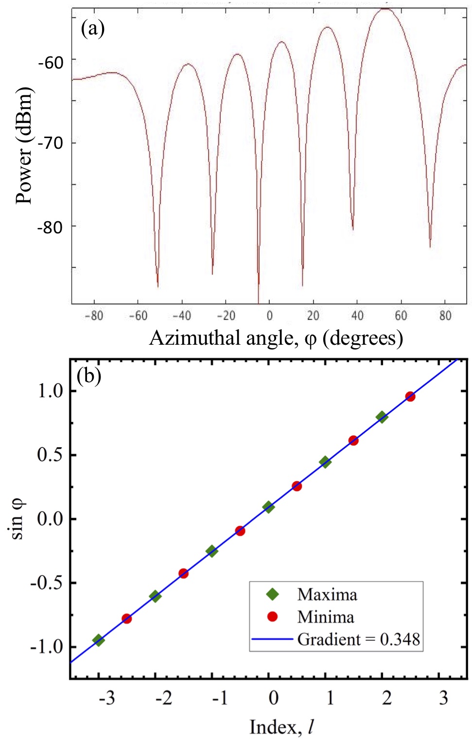
Figure 17: a) Simulated received power versus azimuthal angle $\phi$ for an antenna-to-detector distance of 10.0 m, and subluminal source speed $v/c=0.5$; the antenna simulated is that in Fig. 13(a) and data are shown for $\omega/2\pi=2.5$ GHz. As is the case for the experimental data shown in Fig. 14(a), the simulated power oscillates with azimuthal angle. (b) A plot of $\sin\phi$ versus index $l$, where $\phi$ denotes the angle at which a maximum (blue) or minimum (red) in power occurs, for the numerical data in (a). The gradient of the fitted line is 0.35, very close to the experimental values shown in Fig. 14(b).

X.2 Numerical results

An example of the numerical calculations for constant $v/c$ is compared with experimental data in Fig. 16. The experimental conditions [voltage applied to the electrodes, polarization-current speed $(v/c=4)$, dielectric dimensions- the antenna is that shown in Fig. 13(a)] are used as model input parameters. After correction for the gain of the receiver dipole and cabling used in the experiment, there is a reasonable quantitative match between data and theory, especially close to the main lobe. At larger angles, the match is less good. This is understandable, because the subsidiary minima are very dependent on the precise phases of the signals applied to each antenna element, which are subject to errors of a few degrees in the experiment dissert . Similar quantitative agreement between model and anechoic chamber data was obtained for all speeds above $v/c=2$.

Turning to subluminal speeds, Fig. 17(a) shows a simulation of the antenna shown in Fig 13(a) run at $v/c=0.5$, frequency $\omega/2\pi=2.5$ GHz and for an antenna-to-detector distance of 10 m. The calculated power oscillates with azimuthal angle in a similar manner to the experimental data [see Fig. 14(a)]. Fig. 17(b) plots the $\sin\phi$ versus index $l$ for the model calculation shown in Fig. 17(a); positions of both minima and maxima are shown. The gradient of the fitted line is 0.35, close to the experimental gradients shown in Fig. 14(b).

The results in Figs. 14 [experimental] and 17 [model] may be understood as follows dissert . Ideally, no vacuum Čerenkov radiation should be emitted for $|v/c|<1$, as the emission angle $\sin^{-1}c/v$ becomes imaginary Schott ; Ginzburg . In this context, “ideal” implies an infinitely-long source of identical elements, in which the radiation from all elements superposes to produce no net emission. However, the 32-element antenna shown in Fig. 13(a) is of finite length, so that the radiation measured in the $v/c=0.5$ experiments is likely to come mostly from the ends of the array; the elements at the ends have adjacent elements on only one side. Hence, one might expect that about half of their emitted power would be cancelled out, so that the two end elements behave like a double-slit experiment emitting a total power $\sim(1/2)\times 2\times(1/32)=1/32$ of the total power of the array. Converting into dB, $10\log_{10}(1/32)=-15$ dB, explaining why the peak subluminal emission in both experiment and simulations is $15-20$ dB lower than the peak vacuum Čerenkov power produced at speeds $v/c>2$, where all 32 elements contribute.

Using Eq. 13 with the relevant wavelengths $\lambda=2\pi c/\omega$, the gradients of the experimental data for $\omega/2\pi=2.4$ GHz and 2.6 GHz [Fig. 14(b)] yield $b=370$ mm and $b=360$ mm, and the simulation [$\omega/2\pi=2.5$ GHz; Fig. 17(b)] $b=347$ mm, values that are very close to the 348 mm overall length of the array of 32 elements [Fig. 13(a)]. Moreover, for $v/c=0.5$, the phase difference of elements $j=1$ and $j=32$ is very close to $11\pi$, explaining why the experimental “interference pattern” has minima quite close to the values of $\phi$ given by Eq. 13 dissert .

Examples of simulated emission from propagating pulses produced by driving voltages analogous to that given in Eq 15 are displayed in the main body of the paper.

XI Small region of polarization current in Superluminal Rotation

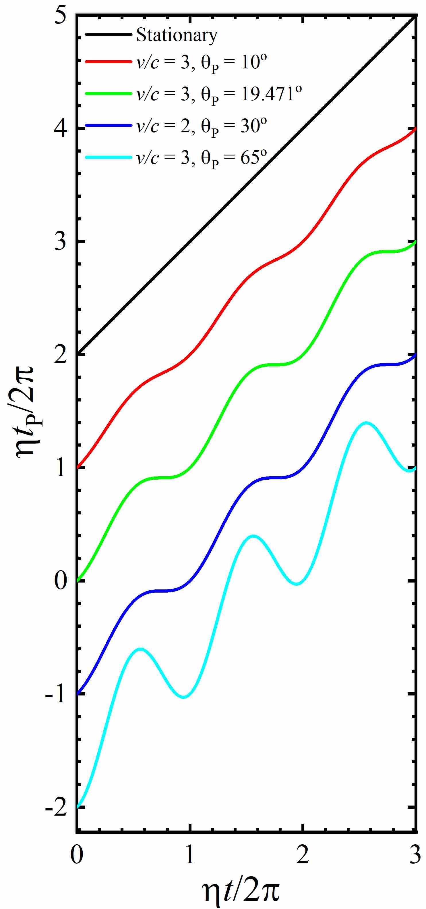
Figure 18: Various forms that Eq. 26 can take depending on the position of the observer (refer to Fig. 19); the times on both axes are scaled by the source angular velocity, $\eta$. The curves are shown for $r_{\rm P}=100r_{\rm L}$, where $r_{\rm L}=c/\eta$ is the light-cylinder radius, and $\varphi_{\rm P}=0$; finite $\varphi_{\rm P}$ merely introduces a phase shift. The observation polar angles $\theta_{\rm P}$ and the source tangential speed $v$ are shown in the inset key. Note that $\theta_{\rm P}=\sin^{-1}(c/v)$ for the green and dark blue curves. Curves are offset by vertical increments of $\eta t_{\rm P}/2\pi=1$ for clarity, and, for reference, the black line shows the $1:1$ correspondence between emission and observation time that would occur for a stationary source. (Curves similar to those shown in light blue and red were first derived in Ref. Schott, ; curves analogous to those shown in green and dark blue are presented in Ref. HA1, .)

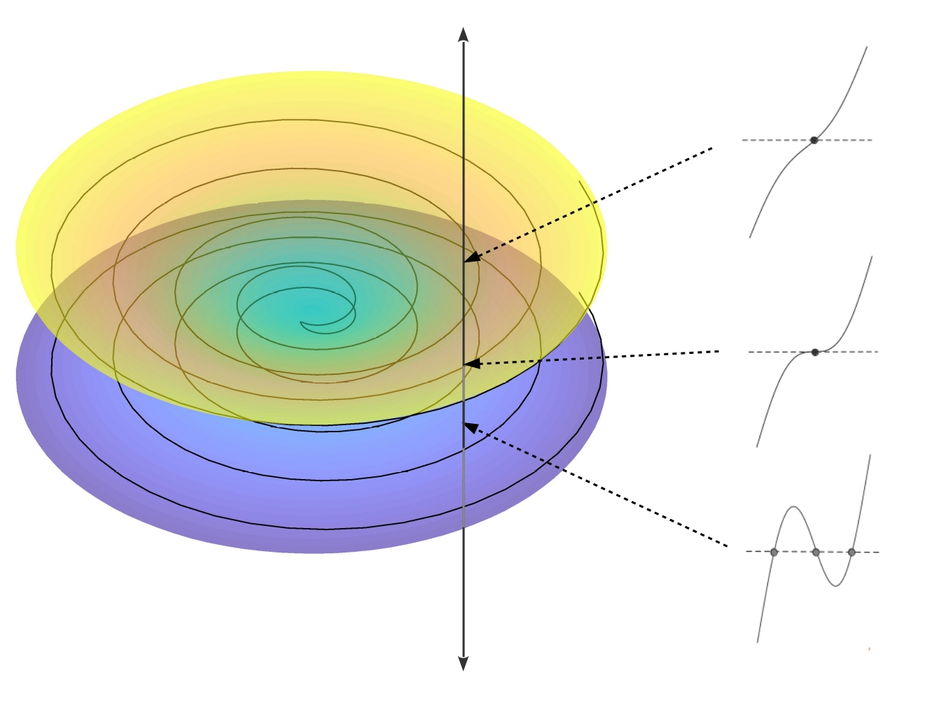
Figure 19: Illustrations of the regions in which Eq. 26 takes the various forms shown in Fig 18. The $z$ axis is vertical, and the circular source orbit lies in the green $(z=0$) plane. The “double-funnel” structure (yellow and purple; symmetrical about the rotation plane $z=0$) represents observer positions at which the source momentarily approaches with an instantaneous speed of $c$ and with zero acceleration. Instantaneous positions of points of this nature are shown as the “spiralling” fine line superimposed on the surface. The shape of Eq. 26 for each region is shown by the curves plotted around the figure, with arrows linking each curve to the place in which it would be observed. The central arrow point lies exactly on the double-funnel structure; the black vertical line traverses the surfaces and is included to clarify the positions of the arrow points. [After Ref. dissert, .]

Consider a polarization-current element of small volume that rotates in the $xy$-plane at radius $r$ with angular velocity $\eta$ and emits radiation (hereafter referred to as the source). In terms of the cylindrical coordinates $r$, $\varphi$ and $z$, the path ${\bf r}(t)=(r,\varphi,z)$ of the source is given by

$$r={\rm const},~{}~{}~{}~{}\varphi=\varphi_{Z}+\eta t,~{}~{}~{}~{}z=0,$$ (23)

where the coordinate $\varphi_{Z}$ denotes the initial azimuthal position of $\varphi$ and is, without loss of generality, assumed to be zero from now on. The wave fronts that are emitted by this point source in an empty and unbounded space can then be described by

$$|{\bf r}_{\rm P}-{\bf r}|=c(t_{\rm P}-t);$$ (24)

as before, the constant $c$ denotes the wave speed and the observation/detection point is defined as $({\bf r}_{\rm P},t_{\rm P})=(r_{\rm P},\varphi_{\rm P},z_{\rm P},t_{\rm P})$. Inserting (23) into (24) and utilizing the theorem of Pythagoras we find that the distance $R$ which separates the source from the observer/detector is given by

$$R(t)=\left[z_{\rm P}^{2}+r_{\rm P}^{2}+r^{2}-2rr_{\rm P}\cos(\varphi_{\rm P}-\eta t)\right]^{\frac{1}{2}}\,.$$ (25)

In consequence, the relationship between the emission time $t$ and the reception (detection) time $t_{\rm P}$ must satisfy

$$t_{\rm P} =t+\frac{R(t)}{c}$$ (26)

$$=t+\frac{1}{c}\left[z_{\rm P}^{2}+r_{\rm P}^{2}+r^{2}-2rr_{\rm P}\cos(\varphi_{\rm P}-\eta t)\right]^{\frac{1}{2}}.$$

Fig. 18 shows the three generic forms that Eq. 26 can take, whilst Fig. 19 identifies the observer positions corresponding to these forms. In the following discussion, it is helpful to define the observer’s polar angle as

$$\theta_{\rm P}=\tan^{-1}\left(\frac{r_{\rm P}}{z_{\rm P}}\right).$$ (27)

First, the green and dark-blue curves in Fig. 18 correspond to an observer positioned on (or very close indeed to) the yellow/purple surface shown in Fig. 19; this surface represents observer positions at which the source momentarily approaches with an instantaneous speed of $c$ and with zero acceleration. The surface can be found (with some effort) by differentiating Eq. 25 and setting $({\rm d}R/{\rm d}t)=-c$ and $({\rm d}^{2}R/{\rm d}t^{2})=0$. With increasingly large distances [$(r_{\rm P}^{2}+z_{\rm P}^{2})^{1/2}\gg r$], the surfaces asymptotically tend to cones with half angles $\theta_{\rm P}=\sin^{-1}(c/v)$, where $v=r\eta$ is the instantaneous (tangential) speed of the source. The green and dark blue curves in Fig. 18 correspond to such an observation angle.

Inside the surface (Fig. 19), plots of Eq. 26 will be similar to the red curve in Fig. 18, whilst outside it, an oscillatory form exemplified by the light blue curve occurs.

The discussion in the final section of the main paper focuses on $t_{\rm P}~{}{\rm versus}~{}t$ curves such as the green and dark blue examples shown in Fig. 18. Apart from a single point at their center where ${\rm d}t_{\rm P}/{\rm d}t=0$, the “steps” are not flat dissert . However, there is a reasonable region of $t$ over which ${\rm d}t_{\rm P}/{\rm d}t\ll 1$.

References

- (1) A. Sommerfeld, Zur Elektronentheorie (3 Teile), Nach. Kgl. Ges. Wiss. Göttingen, Math. Naturwiss. Klasse, 99–130, 363–439 (1904), 201–35 (1905).
- (2) G. A. Schott, Electromagnetic radiation and the mechanical reactions arising from it, Cambridge University Press, 1912.
- (3) V. L. Ginzburg, Vavilov-Čerenkov effect and anomalous Doppler effect in a medium in which wave phase velocity exceeds velocity of light in vacuum, Sov. Phys. JETP, 35 1:92 (1972).
- (4) B. M. Bolotovskii, A. V. Serov, Radiation of superluminal sources in vacuum, Radiation Physics and Chemistry, 75 813 (2006).
- (5) B. M. Bolotovskii, A. V. Serov, Radiation of superluminal sources in empty space, Phys. Usp., 48 903 (2005).
- (6) A. V. Bessarab, A. A. Gorbunov, S. P. Martynenko, N. A. Prudkoi, Faster-than-light EMP source initiated by short X-ray pulse of laser plasma. IEEE Trans. Plasma Sci., 32, 1400 (2004).
- (7) A. V. Bessarab, S. P. Martynenko, N. A. Prudkoi, A. V. Soldatov, V. A. Terenkhin, Experimental study of electromagnetic radiation from a faster-than-light vacuum macroscopic source, Radiation Physics and Chemistry, 75 825 (2006).
- (8) Yu. N. Lazarev, P. V. Petrov, A high-gradient accelerator based on a faster-than-light radiation source, Technical Physics, 45, 971 (2000).
- (9) A. Ardavan, W. Hayes, J. Singleton, H. Ardavan, J. Fopma, and D. Halliday, Corrected Article: “Experimental observation of nonspherically-decaying radiation from a rotating superluminal source J. Appl. Phys. 96, 7760, (2004).
- (10) J. Singleton, A. Ardavan, H. Ardavan, J. Fopma, D. Halliday, and W. Hayes, Experimental demonstration of emission from a superluminal polarization current – A new class of solid-state source for MHz – THz and beyond, Conference Digest of the 2004 Joint 29th International Conference on Infrared and Millimeter Waves and 12th International Conference on Terahertz Electronics, IEEE Cat. No. 04EX857, (2004).
- (11) A. C. Schmidt-Zweifel, Terrestrial and Extraterrestrial Radiation Sources that Move Faster than Light, Master Thesis, 2013, digitalrepository.unm.edu/mathetds/45/. Accessed January 2020.
- (12) John Singleton, Houshang Ardavan, Arzhang Ardavan Apparatus and method for phase fronts based on superluminal polarization current, US Patent number 8125385 (February 2012).
- (13) John Singleton, Lawrence M. Earley, Frank L. Krawczyk, James M. Potter, William P. Romero, Zhi-Fu Wang, Superluminal Antenna, US Patent number 9948011 (February 2012, reissued April 2018).
- (14) Frank Krawczyk, John Singleton, Andrea Caroline Schmidt, Continuous antenna arrays, US Patent, filed August 2018 [USSN 62/721,031
- (15) John Singleton, Andrea Caroline Schmidt Antenna and transceiver for transmitting a secure signal US Patent number 9722724 (August 2017).
- (16) J. D. Jackson, Classical Electrodynamics, Third Edition, John Wiley & Sons, Inc., New York, 1999.
- (17) C. A. Balanis, Advanced Engineering Electromagnetics, Second Edition, John Wiley & Sons, Inc., Hoboken, NY, 2012.
- (18) B. I. Bleaney and B. Bleaney, Electricity and Magnetism. The Oxford Classic Text Edition, Oxford University Press, Oxford, UK, 2013.
- (19) O. D. Jefimenko, Electricity and Magnetism: An Introduction to the Theory of Electric and Magnetic Fields, Second Edition, Electret Scientific, Waynesburg, PA, 1989.
- (20) Philip Willmott, An introduction to synchrotron radiation: techniques and applications, 2nd ed. (Chichester, John Wiley and Sons, 2019).
- (21) See Supplemental Information immediately following this paper for additional experimental and theoretical details.
- (22) Aldo Petosa, Dielectric Resonator Antenna Handbook (Artech House, Boston, 2007).
- (23) Frank Krawczyk, to be published.
- (24) A. C. Schmidt-Zweifel, Theoretical and Experimental Studies of the Emission of Electromagnetic Radiation by Superluminal Polarization Currents. PhD thesis, University of New Mexico, (2020) (available at digitalrepository.unm.edu).
- (25) As mentioned above, the and extent of the antenna are small compared to its length. Therefore we ignore the slight variations in distance caused by the non-zero depth and height of the antenna and represent the motion of the volume-distributed polarization current by a function depending only on and .
- (26) K. Nichols, J. Singleton and A. C. Schmidt-Zweifel, in preparation.
- (27) A.C. Schmidt and J. Singleton, to be published.
- (28) L.C. Godara (ed), Handbook of antennas in wireless communications, (CRC Press, Boca Raton, 2002).
- (29) David L. Adamy, EW 103, Tactical Battlefield Communications – Electronic Warfare (First Edition) (Artech House, Norwood, MA, 2009).
- (30) Kenneth D. Johnston, Analysis of Radio Frequency Interference Effects on a Modern Coarse Acquisition Code Global Positioning System Receiver (Biblioscholar, New York, 2012).
- (31) A. Nordrum and K. Clark, “Everything You Need to Know About 5G”, IEEE Spectrum (27 January, 2017) (https://spectrum.ieee.org – retrieved December 31, 2019)
- (32) 5G Technology Introduction, https://telcomaglobal.com/blog/17780/5g-technology-introduction (retrieved February 01, 2020).
- (33) D. R. Lorimer and M. Kramer, Handbook of Pulsar Astronomy (Cambridge University Press, Cambridge, UK, 2005).
- (34) A. G. Lyne, F. Graham-Smith, Pulsar Astronomy (Cambridge University Press, Cambridge, UK, 2006).
- (35) C. Kalapotharakos, I. Contopoulos, and D. Kazanas, The extended pulsar magnetosphere, Mon. Not. R. Astr. Soc., 420, 2793 (2012).
- (36) I. Contopoulos and C. Kalapotharakos, The pulsar synchrotron in 3D: curvature radiation, Mon. Not. R. Astr. Soc., 404, 767 (2010).
- (37) A. Spitkovsky, Time-dependent Force-free Pulsar Magnetospheres: Axisymmetric and Oblique Rotators, The Astrophysical Journal Letters, 648, 1:51 (2006).
- (38) G.A. Brooker, Modern Classical Optics (Oxford University Press, Oxford, 2003).
- (39) A. Schmidt and J. Singleton, Flaws in the theory of electromagnetic radiation “whose decay violates the inverse-square law”: mathematical and physical considerations, Plasma Physics, submitted.
- (40) H. Ardavan, The mechanism of radiation in pulsars, Mon. Not. R. Astr. Soc., 268, 361 (1994).
- (41) H. Ardavan and J. E. Ffowcs Williams, Violation of the inverse square law by the emissions of supersonically or superluminally moving volume sources, arXiv:astro-ph/9506023v1 (1995).
- (42) H. Ardavan, Generation of focused, nonspherically decaying pulses of electromagnetic radiation, Phys. Rev. E, 58, 6659 (1998).