Data-driven topology optimization of spinodoid metamaterials with seamlessly tunable anisotropy

Abstract

We present a two-scale topology optimization framework for the design of macroscopic bodies with an optimized elastic response, which is achieved by means of a spatially-variant cellular architecture on the microscale. The chosen spinodoid topology for the cellular network on the microscale (which is inspired by natural microstructures forming during spinodal decomposition) admits a seamless spatial grading as well as tunable elastic anisotropy, and it is parametrized by a small set of design parameters associated with the underlying Gaussian random field. The macroscale boundary value problem is discretized by finite elements, which in addition to the displacement field continuously interpolate the microscale design parameters. By assuming a separation of scales, the local constitutive behavior on the macroscale is identified as the homogenized elastic response of the microstructure based on the local design parameters. As a departure from classical FE²-type approaches, we replace the costly microscale homogenization by a data-driven surrogate model, using deep neural networks, which accurately and efficiently maps design parameters onto the effective elasticity tensor. The model is trained on homogenized stiffness data obtained from numerical homogenization by finite elements. As an added benefit, the machine learning setup admits automatic differentiation, so that sensitivities (required for the optimization problem) can be computed exactly and without the need for numerical derivatives – a strategy that holds promise far beyond the elastic stiffness. Therefore, this framework presents a new opportunity for multiscale topology optimization based on data-driven surrogate models.

1 Introduction

Supported by developments in advanced manufacturing, mechanical metamaterials with tunable microstructure and controllable properties have made significant strides towards realizing materials by design (Gibson et al., 2010; Evans et al., 2010; Lee et al., 2012; Zheng et al., 2014; Meza et al., 2014; Berger et al., 2017). Despite all progress, key challenges have persisted, which can be exemplified by truss-, plate-, and shell-based cellular materials, which have dominated the design of metamaterials over the past decade. Most truss-based architectures exhibit poor scaling of stiffness and strength with relative density due to bending deformation of struts (Meza et al., 2017). Plate-based designs exhibit improved stiffness with relative density than trusses and have been shown to reach upper bounds on the achievable effective stiffness of cellular media (Berger et al., 2017; Tancogne-Dejean et al., 2018). However, both types of architectures suffer from stress localization at the junctions of beams or plates, which results in early failure and poor recoverability (Portela et al., 2018; Mateos et al., 2019; Latture et al., 2018). Smooth architectures like those based on triply-periodic minimal surfaces (TPMS) (Nguyen et al., 2017; Han et al., 2017; Al-Ketan and Abu Al-Rub, 2019) address the aforementioned issue, but they do not overcome a common limitations in the fabrication of architectures based on periodic unit cells: classically, all truss, plate, and TPMS designs produce periodic structures with high sensitivity of mechanical properties to symmetry-breaking imperfections and defects and limited opportunity for introducing smoothly spatially variant structures.

In light of these challenges, spinodal metamaterials have emerged recently as a new class of non-periodic architected . Their design is inspired by topologies observed during spinodal decomposition (Cahn, 1961; Allen, 2001), which occurs, e.g., during rapid diffusion-driven phase separation in nanoporous alloys (Erlebacher et al., 2001; Hodge et al., 2007), polymer blends (Bruder and Brenn, 1992), and micro-emulsions (Lee and Mohraz, 2010). The computational design of spinodal microstructures relies on simulating the phase separation process by phase field methods whose kinetics are modeled by Cahn-Hilliard-type evolution equations (Cahn and Hilliard, 1958; Cook, 1970; Stewart and Goldenfeld, 1992; Torabi et al., 2009; Salvalaglio et al., 2015; Vidyasagar et al., 2018; Vuijk et al., 2019) or, as a shortcut, by Gaussian random fields (Soyarslan et al., 2018). As a two-phase mixture spontaneously decomposes into two spatially-separated stable phases, the process is artificially arrested and solid- or shell-based topologies are extracted by, respectively, removing one of the two phases or by retaining the interfaces and eliminating both phases. The resulting topologies are composed of smooth, bi-continuous, and non-self-intersecting surfaces Spinodal metamaterials can also self-assemble across several length scales – from centimeters to nanometers (Portela et al., 2020), which is a promising avenue to overcome the scalability challenge of additive manufacturing.

We recently introduced a computational shortcut to generate spinodal-like topologies, referred to as spinodoid topologies (Kumar et al., 2020a). This approach replaces computationally expensive phase field simulations for topology generation and provides a simple parametrization based on anisotropic Gaussian random fields (GRFs) (Adler and Taylor, 2007; Cahn, 1965); unlike the isotropic formulation of Soyarslan et al. (2018), spinodoids allow for an efficient exploration of a wide design space of anisotropic mechanical properties. When designing functionally-graded metamaterials, the GRF-based approach admits seamless, spatially-variant topologies, which in contrast to periodic unit-cell-based designs bypasses discontinuities and tessellation-related limitations.

Spinodoid metamaterials bear potential for applications ranging from energy absorption and impact protection to heat exchange and to synthetic bone. An ongoing challenge in the design of patient-specific bone implants is to match the anisotropic topological and mechanical properties of bone – which can be highly heterogeneous across patients as well as within the same bone. Functionally-graded spinodoid metamaterials were shown to be promising candidates for inverse-designed synthetic bones (Kumar et al., 2020a) for improved biomechanical compatibility and reduced bone atrophy. Yet, aside from optimizing the properties of specific spinodoid topologies, they have not been used in any two-scale design challenge, such as, e.g., identifying the optimal macroscale shape of a bone implant while optimizing the local, spatially-varying spinodoid microstructure. To this end, we here address the systematic design of spatially-variant, functionally-graded bodies with a spinodoid microstructure through a data-driven topology optimization approach.

Topology optimization is a well-established technique (see Bendsoe and Sigmund (2013) and Sigmund and Maute (2013) for detailed reviews). The classical Solid Isotropic Material Penalization (SIMP) method and its extensions (Bendsoe and Kikuchi, 1988; Bendsøe, 1989; Sigmund and Petersson, 1998; Bendsøe and Sigmund, 1999; Sigmund, 2001) define a continuous volume fraction field $\rho:\Omega\to[0,1]$ over a body $\Omega\subset\mathbb{R}^{d}$ in $d$ dimensions, such that the local linear elastic modulus tensor is approximated as

$$\mathbb{C}=\mathbb{C}_{0}+(\mathbb{C}_{S}-\mathbb{C}_{0})\rho^{p},$$ (1)

where $\mathbb{C}_{0}$ and $\mathbb{C}_{S}$ are the stiffness tensors of void and solid regions, respectively, and $p\geq 3$ is a penalization exponent to promote (approximately) purely void or solid states. Most SIMP-based methods optimize the material distribution within a macroscopic body, e.g., obtaining the fill-fraction field $\rho(\bm{x})$ for all $\bm{x}\in\Omega$ by minimization of the total compliance subject to given boundary conditions and loads.

Multiscale topology optimization additionally focuses on the microscale design (e.g., optimizing the architecture of a metamaterial, or the fiber orientation in composites) in a spatially-variant fashion along with the material distribution on the macroscale (unlike, e.g., multiresolution approaches which gain efficiency by introducing different mesh resolutions on the same (macro-)scale (Nguyen et al., 2010)). The two-scale optimization may be carried out sequentially (Schury et al., 2012; Zowe et al., 1997) – e.g., identify optimal material stiffness tensor fields for the macroscale problem and then search the microstructural design space to meet the target properties using inverse homogenization methods (Sigmund, 1994, 1995). In practice, this approach faces challenges because the target material properties may be physically infeasible or unachievable by the chosen microstructural design space. As a remedy, simultaneous optimization at both scales (e.g., in an FE² setting) is more robust (Rodrigues et al., 2002; Coelho et al., 2008; Xia and Breitkopf, 2014) but also computationally expensive. Here, we adopt the latter approach of simultaneous two-scale optimization in a new, computationally efficient fashion.

Topology optimization with anisotropic materials allows for manipulating the material orientation to generate structures with superior properties. In the context of compliance minimization problems, several works have shown that optimal orientations of anisotropic materials tend to align with the principal stress or strain directions (Suzuki and Kikuchi, 1991; Gibiansky and Cherkaev, 2018; Diaz and Bendsøe, 1992; Pedersen, 1989, 1990, 1991; Gao et al., 2012; Stegmann and Lund, 2005; Groen et al., 2019). Within two-scale topology optimization, such alignment can be achieved by treating, e.g., the orientation angle(s) as additional design variables, which in composites is also known as continuous fiber angle optimization (CFAO) (Jiang et al., 2019; Xia and Shi, 2017; Setoodeh et al., 2005; Nomura et al., 2015). In most such approaches, the inherent anisotropy of the base material is assumed constant. By contrast, recent works (Sivapuram et al., 2016; Gao et al., 2019; Watts et al., 2019; White et al., 2019) optimized the material anisotropy by tuning the microstructural architecture; yet, they did not consider the (spatially varying) orientation of the microstructure in a macroscopic body – primarily because such designs are based on periodic unit cells, which do not admit tessellations with arbitrary and/or spatially-variant orientations. For example, the optimized strut-based cuboidal unit-cells of Watts et al. (2019) are always aligned with the Cartesian coordinate axes, which is sub-optimal compared to the case when the cells and the constituent struts are aligned locally with the principal stress or strain directions. Recently, Wu et al. (2019) introduced conforming lattice optimization to address this issue; however, their strut-based design domain (rectangular or cuboidal cells with beams at the edges) strongly limits the microstructural and anisotropic tunability. Distinct from the above works with either fixed material anisotropy or fixed material orientation, our spinodoid topologies discussed here are simultaneously optimized for both the material anisotropy as well as the orientation distribution of the microstructure within a macroscopic body.

When designing metamaterials with spatially varying microstructure, multiscale topology optimization is computationally expensive, as on-the-fly homogenization methods using, e.g., the finite element method (FEM) must extract the effective properties at each material point on the macroscale from the underlying, local microstructure in each iteration of the optimization problem. Look-up tables are a convenient short-cut (Schumacher et al., 2015), yet they strongly limit the available design space and raise questions about interpolations between available data. More recently, machine learning (ML) techniques have attracted interest for accelerating topology optimization in two ways. First, by creating a dataset of solutions obtained using conventional multiscale topology optimization for several different boundary conditions, loads, microstructures, and material properties, a data-driven model can be learned for accelerated or even real-time prediction of the optimal solution as a function of these inputs without the need for an optimizer (Ulu et al., 2016; Sosnovik and Oseledets, 2019; Banga et al., 2018; Lei et al., 2019; Yu et al., 2019; Zhang et al., 2019a). However, since these approaches are essentially image-to-image learning (e.g., treating the boundary conditions or material distribution as multi-channel images), a large amount of training data is required to achieve reasonable accuracy. Additionally, generalization to unseen inputs (e.g., new loads or boundary conditions) is limited. The above methods are further challenging to extend to three-dimensional (3D) multiscale optimization with high-dimensional design parametrizations.

Second, topology optimization has been accelerated by employing homogenization surrogate models, which are typically developed through an offline training or interpolation of structure-property tables. For example, Watts et al. (2019) developed polynomial surrogate models of homogenized elastic properties of open-truss micro-architectures for deployment in multiscale topology optimization. Others have used Gaussian processes (Zhang et al., 2019b), Numerical EXplicit Potentials (NEXP) (Xia and Breitkopf, 2015; Yvonnet et al., 2009), and single-layer neural networks (NNs) (White et al., 2019) in related contexts to approximate the effective material response to bypass expensive FEM simulations. However, complex design spaces like that of spinodoids (which have high-dimensional, highly-nonlinear, and multiply-connected parametrization domains) require surrogate models beyond simple interpolation methods. To this end, we employ deep NNs (DNNs), which have emerged as powerful tools to efficiently learn in high-dimensional spaces. In this contribution, a DNN pre-trained on a structure-property dataset (obtained via FEM) is used to predict the anisotropic elastic stiffness of a given spinodoid topology.

In this study, we present a multiscale topology optimization framework for cellular structures based on spinodoid topologies, with simultaneous optimization of the macroscale material distribution and the microstructural (spinodoid) design and orientation, where the effective microscale response and associated sensitivities are provided by a data-driven surrogate model that replaces nested FE calculations on the microscale. We point out that the optimization problem requires computing the sensitivity of the compliance at a material point on the macroscale with respect to its design parameters. Lacking closed-form derivatives, this sensitivity analysis in our multiscale description requires numerical differentiation (ND), which involves perturbing the design parameters and recomputing the effective stiffness for each perturbation – requiring computationally expensive FE calculations. Moreover, its accuracy is strongly subject to round-off and truncation errors. While symbolic differentiation (SD) of the surrogate model can give exact derivatives, it leads to inefficient and redundant expressions when applied to complex nonlinear functions as is the case here. We address this issue by using automatic differentiation (AD), which is naturally supported by our NN-based surrogate model. Distinct from ND and SD, AD avoids the above limitations by creating a computational graph that tracks the series of mathematical operations between the inputs and outputs of an arbitrary function and applying chain rule recursively to compute its derivatives. Note that the derivatives are exact, even though AD does not provide the functional form of the derivatives like SD. An extensive introduction to AD can be found in Griewank and Walther (2008). Examples of application of AD to design optimizations can be found in, e.g., Su and Renaud (1997); Barthelemy and Hall (1995); Charpentier (2012); White et al. (2019).

In the following, we present the topology generation and homogenization of spinodoids in Section 2. Section 3 defines the multiscale topology optimization problem, for which Section 4 introduces the DNN-based surrogate model and discusses its implementation in topology optimization. We use this model in Section 5 to present several benchmark examples of compliance minimization, before Section 6 concludes our study.

2 Spinodoid topologies with tunable anisotropy

2.1 Spinodoid topology generation

Consider a homogeneous two-phase solution occupying a domain $\mathcal{V}\in\mathbb{R}^{3}$ and undergoing spinodal decomposition. During the early stages, the separated phases are spatially-arranged in a stochastic bi-continuous topology, whose evolution is governed by the Cahn-Hilliard equation (Cahn and Hilliard, 1958; Cahn, 1961, 1965). Let $\varphi:\mathcal{V}\to\mathbb{R}$ be the phase field that describes the concentration fluctuation of one phase. Using Fourier analysis, Cahn showed that the phase field can be described by a GRF – a superposition of several plane waves with fixed wavelength but random wave vectors and phase shifts. That is, the concentration $\varphi$ of either of the two phases at $\bm{x}\in\mathcal{V}$ is given by

$$\varphi(\bm{x})=\sqrt{\dfrac{2}{N}}\sum\limits_{i=1}^{N\gg 1}\cos\left(\beta\bm{n}_{i}\cdot\bm{x}+\gamma_{i}\right),$$ (2)

where $N$ is the number of waves, $\beta>0$ is a constant wavenumber, and $\bm{n}_{i}\sim\mathcal{U}(S^{2})$ and $\gamma_{i}\sim\mathcal{U}\left([0,2\pi)\right)$ denote the uniformly-distributed direction and phase angle of the $i^{\text{th}}$ wave vector, respectively. Without loss of generality, the amplitudes are assumed equal and constant to ensure that $\varphi$ is normally distributed with zero mean and unitary standard deviation. Note that $\beta$ prescribes a wavelength and hence directly controls the microstructural length scale.

The GRF in (2) describes the separated phases in the case of isotropic diffusion, whereas direction-dependent, anisotropic topologies are generally the result phase separation processes with directional preference in interfacial energy or diffusive mobility – which translates into a directional preference in the distribution of the wave vectors in (2). Here, we follow the anisotropic extension of Cahn’s GRF solution presented in Kumar et al. (2020a). Assuming the principle directions of mobility are aligned with the Cartesian basis $\{\hat{\bm{e}}_{1},\hat{\bm{e}}_{2},\hat{\bm{e}}_{3}\}$, the resulting anisotropic topologies can be approximated by a non-uniform orientation distribution function (ODF) parameterized by

$$\bm{n}_{i}\sim\mathcal{U}\left(\left\{\bm{k}\in S^{2}:\left(|\bm{k}\cdot\hat{\bm{e}}_{1}|>\cos\theta_{1}\right)\oplus\left(|\bm{k}\cdot\hat{\bm{e}}_{2}|>\cos\theta_{2}\right)\oplus\left(|\bm{k}\cdot\hat{\bm{e}}_{3}|>\cos\theta_{3}\right)\right\}\right),$$ (3)

such that the wave vectors in (2) are restricted to lie within cone angles $\{\theta_{1},\theta_{2},\theta_{3}\}$ from the orthogonal Cartesian basis vectors (see Figure 1(a)).

For the purpose of topology generation, GRF models bypass the need for expensive simulations of the Cahn-Hilliard equation. Soyarslan et al. (2018) showed that bi-continuous solid-void microstructures can be generated by applying a level set $\varphi_{0}$ to the phase field in (2), such that

$$\xi(\bm{x})=\begin{cases}1&\quad\text{if }\quad\varphi(\bm{x})\leq\varphi_{0}\\ 0&\quad\text{if }\quad\varphi(\bm{x})>\varphi_{0}\end{cases},$$ (4)

where $\xi(\bm{x})=\{1,0\}$ denotes the presence of solid and void, respectively, at $\bm{x}\in\mathcal{V}$. Since $\varphi$ follows a standard normal distribution, the level set $\varphi_{0}$ is defined as the quantile evaluated at the average relative density $\rho$ of the solid phase: $\varphi_{0}=\sqrt{2}\,\text{erf}^{-1}(2\rho-1)$. We note that, while we only consider solid networks for our multiscale topology optimization framework in the following, shell-type architectures can be generated in a similar fashion by choosing an isosurface of $\varphi(\bm{x})=\varphi_{0}$.

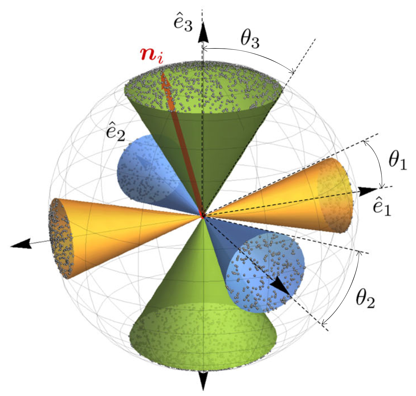
(a) Schematics of the design parameters: $\theta_{1},\theta_{2},\theta_{3}$

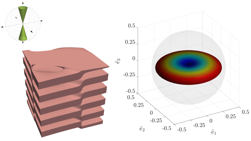
(b) Lamellar: $\rho=0.5,\theta_{1}=0^{\circ},\theta_{2}=0^{\circ},\theta_{3}=15^{\circ}$

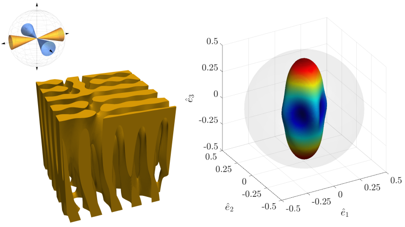
(c) Columnar: $\rho=0.5,\theta_{1}=15^{\circ},\theta_{2}=15^{\circ},\theta_{3}=0^{\circ}$

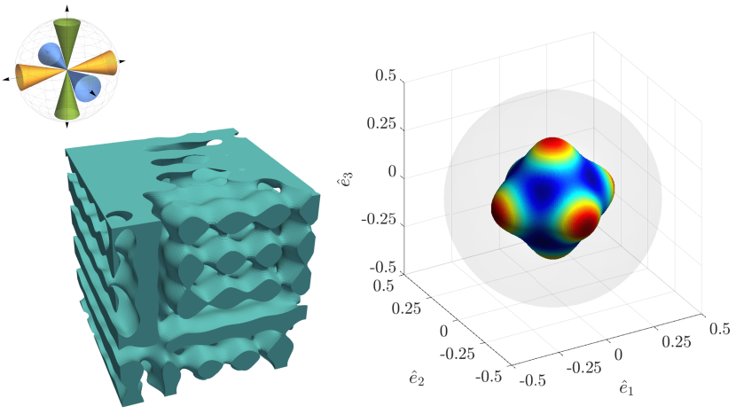
(d) Cubic: $\rho=0.5,\theta_{1}=15^{\circ},\theta_{2}=15^{\circ},\theta_{3}=15^{\circ}$

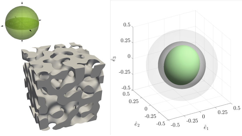
(e) Isotropic: $\rho=0.5,\theta_{1}=90^{\circ},\theta_{2}=90^{\circ},\theta_{3}=90^{\circ}$

Figure 1: Spinodoid topology generation and representative examples. (a) Schematic illustration of the three cone angles $\theta_{1}$, $\theta_{2}$, and $\theta_{3}$, which describe the anisotropic distribution of wave vectors $\bm{n}_{i}$. (b-e) Examples of spinodoid topologies with their respective anisotropic elasticity surfaces (and an illustration of the cone angles indicated in each caption). Each point on the elasticity surface denotes the Young’s modulus in the corresponding direction. Light and dark gray spheres indicate, respectively, the elastic Voigt upper bound and the Hashin-Shtrikman upper bound (the latter being applicable only to the isotropic structure). Adapted from Kumar et al. (2020a).

Solid spinodoid topologies are hence characterized by the set of design parameters $\bm{\Theta}=(\rho,\theta_{1},\theta_{2},\theta_{3})^{\mathrm{T}}$, which provide a way to control the porosity and anisotropy of the architecture. To avoid disjoint solid domains, the design parameters are bounded to $\rho\geq\rho_{\text{min}}$ and $\theta_{1},\theta_{2},\theta_{3}\in\{0\}\cup[\theta_{\text{min}},\pi/2]$. In subsequent numerical examples we choose $\rho_{\text{min}}=0.3$ and $\theta_{\text{min}}=\pi/6$. The resulting anisotropic topologies can be broadly categorized into lamellar, columnar, and cubic types (Figure 1), and they are obtained when, respectively, one, two, or three of the angles $\{\theta_{1},\theta_{2},\theta_{3}\}$ are non-zero.

2.2 Homogenization of the elastic stiffness

For a given set of design parameters, we use via FEM to compute the effective mechanical stiffness of the corresponding spinodoid topology. We consider a cubic representative volume element (RVE), in which the GRF from (2) with level set (4) is used to generate a spinodoid architecture. The base material of the solid is assumed homogeneous, isotropic, linear elastic with Young’s modulus $E_{s}$ and Poisson’s ratio and $\nu_{s}=0.3$ ($E_{s}$ is arbitrary as it scales linearly with the effective stiffness). For an RVE of size $l\times l\times l$, the wave number $\beta=10\pi/l$ was found to be . Six numerical experiments are performed on the RVE, one uniaxial stretch and one simple-shear loading along each of the three principal axes. By applying average strains $\langle\bm{\varepsilon}\rangle$ to the RVE for each of the six cases, the elastic stiffness tensor $\hat{\mathbb{C}}$ is computed by solving the linear system of equations $\langle\bm{\sigma}\rangle=\hat{\mathbb{C}}\,\langle\bm{\varepsilon}\rangle$, where $\langle\bm{\sigma}\rangle=\frac{1}{|\mathcal{V}|}\int_{\mathcal{V}}\bm{\sigma}\;\!\mathrm{d}V$ is the volume-averaged stress obtained from FEM. Since the spinodoid topologies lack periodicity, we apply affine boundary conditions to the RVE and acknowledge that the computed response provides an upper bound to the actual effective stiffness (yet, spinodoids – like spinodals – retrieve their beneficial stiffness scaling properties from being stretching-dominated, so that affine boundary conditions can be expected to not affect the response as much as in, e.g., bending-dominated trusses).

The fourth-order stiffness tensor is visualized through the elastic surface, showing Young’s modulus $E(\bm{d})$ along all directions $\bm{d}\in S^{2}$, which is computed as

$$E(\bm{d})=\bigg{(}\sum\limits_{i,j,k,l=1}^{3}\hat{\mathbb{C}}_{ijkl}^{-1}d_{i}d_{j}d_{k}d_{l}\bigg{)}^{-1}.$$ (5)

Figure 1 illustrates representative examples of the diverse anisotropic stiffnesses achievable by the spinodoid design space – from lamellar topologies (being highly soft in a dedicated direction) to columnar ones (stiff in two directions) to cubic and (approximately) isotropic topologies. In subsequent derivations, the strain, stress, and stiffness tensors will be used frequently in their respective Voigt notations, which we denote by subscript $(\cdot)_{v}$. For further details on topology generation and homogenization of spinodoids, the reader is referred to Kumar et al. (2020a).

3 Multiscale topology optimization

The overall multiscale topology optimization setup presented in the following is schematically summarized in Figure 2.

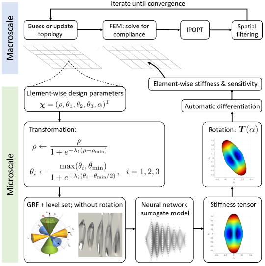
Figure 2: Schematic illustration of the topology optimization framework for spinodoid metamaterials.

3.1 Macroscale: boundary value problem and compliance minimization

The classical boundary value problem (BVP) of static equilibrium in a macroscale domain $\Omega\subset\mathbb{R}^{d}$ in $d$ dimensions is given by

$$\operatorname{div}\bm{\sigma}(\bm{u},\bm{\chi})={\bm{0}}\ \ \ \text{in}\ \Omega,\qquad\bm{u}=\tilde{\bm{u}}\ \ \ \text{on}\ \partial\Omega_{u},\qquad\bm{\sigma}\bm{n}=\tilde{\bm{t}}\ \ \ \text{on}\ \partial\Omega\setminus\partial\Omega_{u}.$$ (6)

Here, $\bm{u}:\Omega\to\mathbb{R}^{d}$ denotes the displacement field with essential boundary conditions $\tilde{\bm{u}}$ on the Dirichlet boundary $\partial\Omega_{u}\subseteq\partial\Omega$. $\tilde{\bm{t}}$ denotes the prescribed tractions on the remaining boundary with outward unit normal $\bm{n}$, and $\bm{\sigma}$ is the symmetric infinitesimal stress tensor. For linear elasticity with the linearized strain tensor $\bm{\varepsilon}=\operatorname{sym}(\nabla\bm{u})$, stresses and strains are locally related via $\bm{\sigma}(\bm{x})=\mathbb{C}(\bm{x})\bm{\varepsilon}(\bm{x})$ for $\bm{x}\in\Omega$.

In our two-scale setup, we assume that the local elastic properties and mass density at a point $\bm{x}\in\Omega$ on the macroscale stem from homogenization over a microscale RVE, whose architecture is defined by a local set of design parameters, $\bm{\chi}(\bm{x})$. Assuming a separation of scales, the macroscale stresses $\bm{\sigma}$ and strains $\bm{\varepsilon}$ are related via the linear elastic constitutive relation

$$\bm{\sigma}(\bm{x})=\mathbb{\hat{C}}\big{(}\bm{\chi}(\bm{x})\big{)}\bm{\varepsilon}(\bm{x}),$$ (7)

where $\mathbb{\hat{C}}$ represents the homogenized stiffness tensor obtained from an RVE with design parameters $\bm{\chi}$, so the spatial variability in microstructural topology is captured naturally by $\bm{\chi}(\bm{x})$. Macro- and microscales are hence coupled by exchanging homogenized information such as $\bm{\chi}$ and $\hat{\mathbb{C}}$. For the example of spinodoids, $\bm{\chi}$ includes $\bm{\Theta}=(\rho,\theta_{1},\theta_{2},\theta_{3})^{T}$ among other design parameters which will be explained in Section 3.2.

We use FEM to solve the macroscale BVP (6) in a (Bubnov-)Galerkin setting, which discretizes the macroscale body $\Omega$ into a mesh containing $n$ elements and $n_{n}$ nodes. In subsequent examples, we use constant-strain tetrahedra in 3D, having a single quadrature point per element. Of course, the following formulation can be analogously adopted for higher-order elements. Let $\mathcal{X}=\{\bm{\chi}^{e},e=1,\dots,n\}$ be the set of all microstructural design parameters (one such set for each element $e$), such that the stiffness matrix of element $\Omega^{e}$ is given by

$$\bm{k}^{e}(\bm{\chi}^{e})=\int_{\Omega^{e}}({\bm{B}^{e}})^{\mathrm{T}}\mathbb{\hat{C}}_{v}(\bm{\chi}^{e})\bm{B}^{e}\;\!\mathrm{d}\Omega,$$ (8)

where $\bm{B}^{e}$ denotes the strain-displacement matrix of element $e$ (Cook et al., 2001). For given $\mathcal{X}$, the global vector of nodal displacements $\bm{U}=\{\bm{u}_{i},i=1,\ldots,n_{n}\}$ is obtained from the following system of equations (assuming that essential boundary conditions have been imposed):

$$\bm{K}(\mathcal{X})\bm{U}(\mathcal{X})=\bm{F}.$$ (9)

The global displacement vector $\bm{U}$, global stiffness matrix $\bm{K}$, and the external force vector $\bm{F}$ are obtained via assembly of the element-wise displacement vectors $\bm{u}^{e}$, element stiffness matrices $\bm{k}^{e}$, and external forces (derived for each element from the applied tractions $\tilde{\bm{t}}$), respectively.

The total compliance at the macroscale is given by

$$\Phi(\mathcal{X})=\bm{U}(\mathcal{X})\cdot\bm{F}=\bm{U}(\mathcal{X})\cdot\bm{K}(\mathcal{X})\bm{U}(\mathcal{X})=\sum_{e=1}^{n}{\bm{u}^{e}}\cdot\bm{k}^{e}\bm{u}^{e}=\sum_{e=1}^{n}{\bm{u}^{e}}\cdot\left(\int_{\Omega^{e}}(\bm{B}^{e})^{\mathrm{T}}\mathbb{\hat{C}}_{v}(\bm{\chi}^{e})\bm{B}^{e}\;\!\mathrm{d}\Omega\right)\bm{u}^{e},$$ (10)

where (8) and (9) have been substituted. The compliance minimization problem on the macroscale is formulated as

$$\min_{\mathcal{X}}\Phi(\mathcal{X}),\quad\text{subject to}\quad\frac{1}{|\Omega|}\int_{\Omega}\rho\;\!\mathrm{d}V\leq\bar{\rho}\quad\text{and}\quad\text{\eqref{eq:KU=F}},$$ (11)

where $\bar{\rho}$ prescribes a target on the overall relative density at the macroscale (effectively imposing a total weight constraint), and (9) ensures static equilibrium of the loaded structure.

The nonlinear optimization problem in (11) is solved using IPOPT (Wächter and Biegler, 2006), a primal-dual interior-point algorithm with a filter line-search method. IPOPT requires sensitivity information, i.e., the derivative of the compliance $\Phi$ with respect to the design parameters $\mathcal{X}$, for determining the line search direction. Differentiating both sides of the equilibrium constraint (9) with respect to $\mathcal{X}$ and noting that $\bm{K}$ is symmetric, we obtain

$$\frac{\partial\bm{K}(\mathcal{X})\bm{U}(\mathcal{X})}{\partial\mathcal{X}}=0\qquad\Rightarrow\qquad\bm{K}\frac{\partial\bm{U}}{\partial\mathcal{X}}=-\frac{\partial\bm{K}}{\partial\mathcal{X}}\bm{U}\quad\text{and}\quad\frac{\partial\bm{U}}{\partial\mathcal{X}}\cdot\bm{K}=-\bm{U}\cdot\frac{\partial\bm{K}}{\partial\mathcal{X}}.$$ (12)

The compliance sensitivity hence follows as

$$\frac{\partial\Phi}{\partial\mathcal{X}}=\frac{\partial\bm{U}\cdot\bm{K}\bm{U}}{\partial\mathcal{X}}=-\bm{U}\cdot\frac{\partial\bm{K}}{\partial\mathcal{X}}\bm{U},$$ (13)

where (12) has been substituted to obtain the right-hand side. Using (10), the above may be expressed as an element-wise summation, viz.

$$\dfrac{\partial\Phi}{\partial\mathcal{X}}=-\sum_{e=1}^{n}{\bm{u}^{e}}\cdot\left(\int_{\Omega^{e}}(\bm{B}^{e})^{\mathrm{T}}\frac{\partial\mathbb{\hat{C}}_{v}(\bm{\chi}^{e})}{\partial\bm{\chi}^{e}}\bm{B}^{e}\;\!\mathrm{d}\Omega\right)\bm{u}^{e},$$ (14)

where $\partial\mathbb{\hat{C}}_{v}(\bm{\chi}^{e})/\partial\bm{\chi}^{e}$ is the element-wise or microscale stiffness sensitivity.

To eliminate numerical instabilities such as checkerboard patterns, we impose a minimum length scale by a filtering technique. Commonly used filter techniques include density filters Bruns and Tortorelli (2001), sensitivity filters Sigmund (1997), and morphology-based filters Sigmund (2007). In our approach, the stiffness sensitivity in (14) is replaced by (no summation over $i$ implied)

$$\frac{\partial\mathbb{\hat{C}}_{v}(\bm{\chi}^{e})}{\partial\chi^{e}_{i}}\leftarrow\left(\displaystyle\sum_{e^{\prime}=1}^{n}w\left(\bm{x},\bm{x}^{e^{\prime}}\right)\chi^{e^{\prime}}_{i}\frac{\partial\mathbb{\hat{C}}_{v}(\bm{\chi}^{e^{\prime}})}{\partial\chi^{e^{\prime}}_{i}}\right)\left(\chi^{e}_{i}\displaystyle\sum_{e^{\prime}=1}^{n}w\left(\bm{x},\bm{x}^{e^{\prime}}\right)\right)^{-1}$$ (15)

with weight function

$$w\left(\bm{x},\bm{x}^{e^{\prime}}\right)=\max\left(0,r_{\text{filter}}-\left\|\bm{x}^{e}-\bm{x}^{e^{\prime}}\right\|\right),$$ (16)

where $\bm{x}\in\Omega^{e}$, while $\bm{x}^{e}$ denotes the position of the center of element $e$, and $r_{\text{filter}}>0$ is a cut-off radius that controls the length scale of the filter.

The optimal solution of (11) yields the set of spatially-varying design parameters $\mathcal{X}$, which can be used to generate the multiscale topology with fully resolved microstructures. Details on the computational generation of fully resolved topologies are presented in A.

3.2 Microscale: spinodoid microstructures

The spinodoid microstructure at every point $\bm{x}\in\Omega$ on the macroscale depends on design parameters $\bm{\chi}(\bm{x})$. As we are using simplicial elements (with a single quadrature point), we deal with element-wise constant $\bm{\chi}^{e}$. Here, we consider the spinodoid topology within a single element and, for the sake of brevity, we drop the superscript $(\cdot)^{e}$ in the following discussion, while tacitly implying that the microscale description applies for each element $e\in\{1,\dots,n\}$. For spinodoids, the microscale response is generally determined by design parameters $\bm{\chi}=\bm{\Theta}=(\rho,\theta_{1},\theta_{2},\theta_{3})^{\mathrm{T}}$. Unfortunately, this straightforward definition of $\bm{\chi}$ presents technical challenges in the context of multiscale topology optimization, which are addressed here.

As discussed in Section 2, the spinodoid design space is restricted to $\rho\geq\rho_{\text{min}}$ to avoid disjoint solid domains (at the microscale). With this constraint, however, the entire macroscale domain is filled with material ($\rho>0$). As a remedy, we need to introduce macroscale holes by allowing $\rho=0$ in the (macroscale) voids, while enforcing $\rho\geq\rho_{\text{min}}$ in the non-void regions. . Similar to the density $\rho$, the domain for angles $\theta_{1},\theta_{2},\theta_{3}\in\{0\}\cup[\theta_{\text{min}},\pi/2]$ is also disjoint. From an optimization perspective, such disjoint parameter spaces are not favorable. Therefore, we transform the parameter space in a continuous fashion by defining the transformation (Figure 4)

$$\bm{f}(\bm{\Theta})=\left(\dfrac{\rho}{1+e^{-\lambda_{1}(\rho-\rho_{\text{min}})}},\dfrac{\max(\theta_{1},\theta_{\text{min}})}{1+e^{-\lambda_{2}(\theta_{1}-\theta_{\text{min}}/2)}},\dfrac{\max(\theta_{2},\theta_{\text{min}})}{1+e^{-\lambda_{2}(\theta_{2}-\theta_{\text{min}}/2)}},\dfrac{\max(\theta_{3},\theta_{\text{min}})}{1+e^{-\lambda_{2}(\theta_{3}-\theta_{\text{min}}/2)}}\right)^{\mathrm{T}}\qquad\text{with}\quad\lambda_{1},\lambda_{2}\gg 1.$$ (17)

Here, each transformation is a smooth approximation of a Heaviside step function , which continuous parameter spaces $\rho\in[0,1]$ and $\theta_{1},\theta_{2},\theta_{3}\in[0,\pi/2]$ when replacing $\bm{\Theta}$ by $\bm{f}(\bm{\Theta})$ in the topology optimization problem. The smoothness, controlled by $\lambda_{1}$ and $\lambda_{2}$, is necessary to ensure that gradient-based optimization methods such as IPOPT are applicable. The disallowed parameter values are approximately mapped to the closest allowed values. For example, using $\bm{f}(\bm{\Theta})$ relaxes the bounds on the relative density to $\rho\in[0,1]$, as microstructures with $\rho<\rho_{\text{min}}$ are effectively mapped to void with zero stiffness. When weight or compliance minimization is the objective, this will force the density to be either zero (void) or greater than $\rho_{\text{min}}$ (spinodoid).

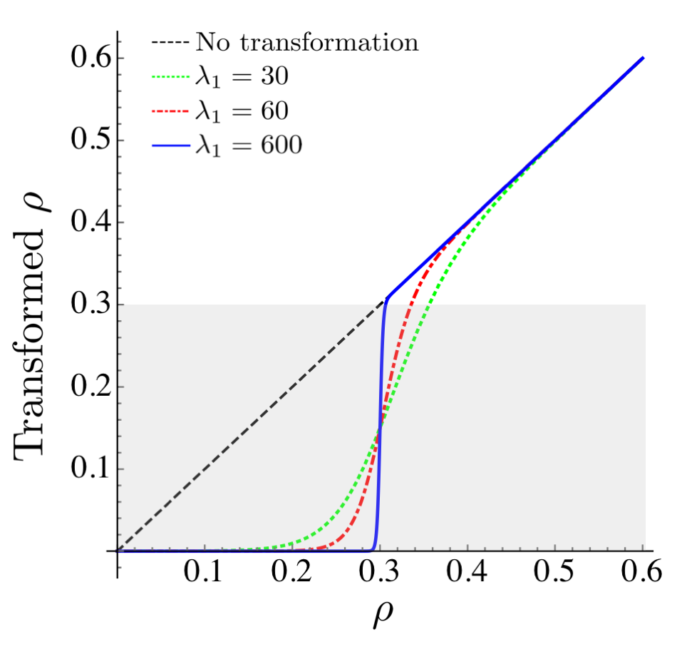
(a)

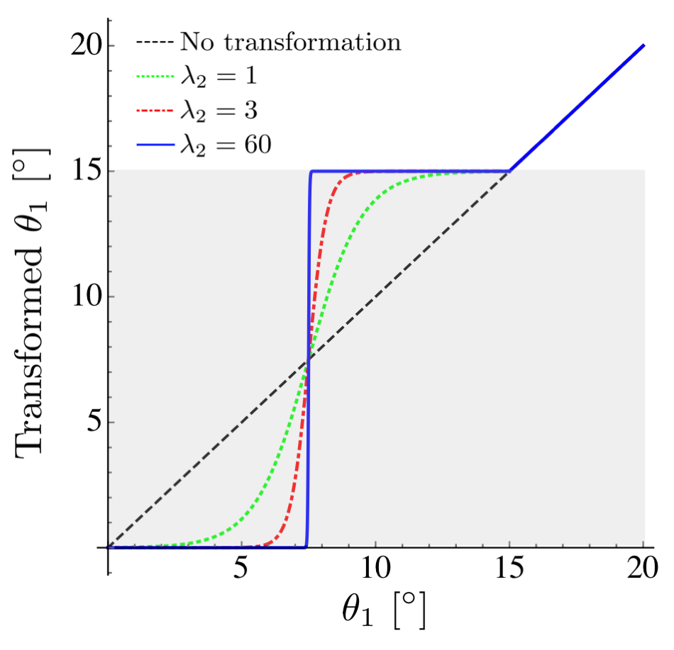
(b)

      

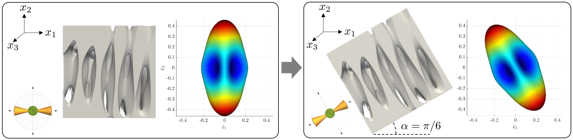
Figure 3: Transformation of the design parameters (a) $\rho$ and (b) $\theta_{1}$ according to $\bm{f}(\bm{\Theta})$ in (17) for different values of $\lambda_{1}$ and $\lambda_{2}$, introduced to avoid inadmissible values (indicated by the shaded regions corresponding to (a) $\rho_{\min}=0.3$, (b) $\theta_{\min}=15^{\circ}$).

Figure 4: Rotation (with $\alpha=30^{\circ}$) of a representative spinodoid topology ($\rho=0.5,\theta_{1}=15^{\circ},\theta_{1}=0^{\circ},\theta_{3}=15^{\circ}$) and its elasticity surface.

So far, the principal directions of the spinodoid topologies and their inherent mechanical anisotropy are aligned with the fixed Cartesian basis $\{\hat{\bm{e}}_{1},\hat{\bm{e}}_{2},\hat{\bm{e}}_{3}\}$. In this case, the effective stiffness $\hat{\mathbb{C}}$ in (7) is the homogenized stiffness of the microstructure (Section 2.2). As the stiffness is direction dependent, we here further expand the design space by applying rigid-body rotations to the generated spinodoid topologies. For demonstration purposes (and since our subsequent benchmarks are in 2D), we restrict ourselves to rotations about a single axis, while noting that the framework can be extended to general 3D rotations. We introduce an expanded set of design parameters $\bm{\chi}=(\rho,\theta_{1},\theta_{2},\theta_{3},\alpha)^{T}$, where $\alpha\in[-\pi/2,\pi/2]$ denotes the angle of a rigid-body rotation (Figure 4) about the (out-of-plane) $\hat{\bm{e}}_{3}$-axis (due to the two-fold symmetry, rotations with $\alpha$ and $(\pi-\alpha)$ are equivalent). Applying such a rotation transforms the Voigt-notation stiffness matrix according to

$$\mathbb{\hat{C}}_{v}(\bm{\chi})=\bm{T}(\alpha)\mathbb{C}_{v}\left(\bm{f}(\bm{\Theta})\right)\bm{T}^{\mathrm{T}}(\alpha),$$ (18)

where $\mathbb{\hat{C}}_{v}$ is the effective stiffness passed to the macroscale in (7), and $\mathbb{C}_{v}\left(\bm{f}(\bm{\Theta})\right)$ is obtained from microscale homogenization of the spinodoid topology with design parameters $\bm{f}(\bm{\Theta})$. The components of rotation matrix $\bm{T}$ are given by

$$\bm{T}(\alpha)=\begin{bmatrix}\cos^{2}\alpha&\sin^{2}\alpha&0&0&0&2\sin\alpha\cos\alpha\\ \sin^{2}\alpha&\cos^{2}\alpha&0&0&0&-2\sin\alpha\cos\alpha\\ 0&0&1&0&0&0\\ 0&0&0&\cos\alpha&-\sin\alpha&0\\ 0&0&0&\sin\alpha&\cos\alpha&0\\ -\cos\alpha\sin\alpha&\cos\alpha\sin\alpha&0&0&0&\cos^{2}\alpha-\sin^{2}\alpha\end{bmatrix}.$$ (19)

The homogenized stiffness and its sensitivity, which involves computing $\partial\mathbb{C}_{v}(\bm{f}(\bm{\Theta}))/\partial\bm{\Theta}$, are the computational bottlenecks (often computed by ND), especially since IPOPT is an iterative algorithm which requires computing the sensitivity of each element several times during the optimization. This motivates the use of data-driven surrogate models that can accelerate the optimization process.

3.3

4 Data-driven surrogate model

4.1 Bypassing FEM-based homogenization

To bypass the computational expense of repetitive FEM simulations required for the microscale homogenization, we use a DNN-based surrogate model for the on-demand prediction of the homogenized stiffness tensor $\hat{\mathbb{C}}$. Due to the symmetries in the ODF defined in (3), the anisotropic stiffness tensor $\mathbb{C}$ is orthotropic with nine independent elastic moduli, which can be encoded into . The DNN can be interpreted as a composition of several linear and nonlinear transformations that provide a map $\mathcal{F}_{\omega}:\bm{\Theta}\rightarrow\bm{S}$ from the spinodoid design parameters $\bm{\Theta}$ to the compressed representation of the stiffness $\mathbb{C}$.

We use the DNN architecture previously developed by Kumar et al. (2020a), which translates to the composite transformation

$$\mathcal{F}_{\omega}[\bm{\Theta}]=\mathcal{L}_{\omega_{7}}^{32\rightarrow 9}\circ\mathcal{R}\circ\mathcal{L}_{\omega_{6}}^{32\rightarrow 32}\circ\mathcal{R}\circ\mathcal{L}_{\omega_{5}}^{64\rightarrow 32}\circ\mathcal{R}\circ\mathcal{L}_{\omega_{4}}^{64\rightarrow 64}\circ\mathcal{R}\circ\mathcal{L}_{\omega_{3}}^{128\rightarrow 64}\circ\mathcal{R}\circ\mathcal{L}_{\omega_{2}}^{128\rightarrow 128}\circ\mathcal{R}\circ\mathcal{L}_{\omega_{1}}^{4\rightarrow 128}[\bm{\Theta}].$$ (20)

Here, $\mathcal{L}_{\omega_{k}}^{i\rightarrow j}$ denotes the $k^{\text{th}}$ linear layer parametrized by the set of weights and biases $\omega_{k}=\{\bm{A}_{k},\bm{b}_{k}\}$ – and we write $\omega=\{\omega_{i},i=1,\dots,7\}$ – such that any $\bm{z}\in\mathbb{R}^{i}$ is transformed according to

$$\mathcal{L}_{\omega_{k}}^{i\rightarrow j}[\bm{z}]=\bm{A}_{k}\bm{z}+\bm{b}_{k},\quad\text{with}\quad\bm{A}_{k}\in\mathbb{R}^{j\times i},\bm{b}_{k}\in\mathbb{R}^{j}.$$ (21)

$\mathcal{R}(\cdot)=\max(0,\cdot)$ is the rectified linear activation unit (ReLU) that acts element-wise on the input and introduces nonlinearity to the series of linear transformations. The design parameters $\bm{\Theta}$ are mapped into intermediate high-dimensional spaces, where the surrogate model can efficiently and accurately learn the nonlinear relationship to the homogenized stiffness values $\bm{S}$. This is particularly advantageous as the stiffness space is highly disjoint because of the discontinuities in the design space (recall that $\theta_{1},\theta_{2},\theta_{3}\in\{0\}\cup[\theta_{\text{min}},\pi/2]$); e.g., the effective stiffnesses of the lamellar and columnar topologies are quite different (cf. Figure 1).

The above surrogate model is trained on a dataset $\left\{(\bm{\Theta}^{i},\bm{S}^{i}),i=1,\dots,n_{\text{train}}\right\}$ containing $n_{\text{train}}$ pairs of randomly sampled spinodoid design parameters $\bm{\Theta}$ and their corresponding homogenized stiffnesses $\bm{S}$ (obtained via FEM). The optimal DNN parameters are obtained using back-propagation and the Adaptive Moment Estimation (Adam) (Kingma and Ba, 2014) to minimize the mean squared prediction error over the training data

$$\omega\leftarrow\arg\min_{\omega}\frac{1}{n_{\text{train}}}\sum_{i=1}^{n_{\text{train}}}\|\mathcal{F}_{\omega}[\bm{\Theta}^{i}]-\bm{S}^{i}\|^{2}.$$ (22)

Once trained, the DNN-based surrogate provides accurate stiffness predictions instantly compared to several minutes for FEM-based homogenization (for the meshes used in our study). As the focus here is on its integration into the multiscale topology optimization framework, we refer the interested reader to Kumar et al. (2020a) for further details pertaining to the architecture, training, and dataset of the DNN surrogate model.

4.2 Bypassing ND for sensitivity computations

The DNN-based surrogate model beneficially provides the sensitivity of the stiffness with respect to the design parameters – an essential information for the multiscale topology optimization. Conventional approaches based on ND that perturb the design parameters are computationally expensive (requiring extensive FEM-based homogenization simulations) and prone to stability and precision issues. In contrast, our DNN-based surrogate model admits inexpensive computations of the sensitivity information, i.e., $\mathcal{F}_{\omega}^{\prime}[\bm{\Theta}]=\partial\bm{S}/\partial\bm{\Theta}$, which can be rearranged tensorially into $\partial\hat{\mathbb{C}}_{v}/\partial\bm{\Theta}$. Since each transformation in the DNN (20) is differentiable almost everywhere, the sensitivity is easily computed by propagating the gradients from $\bm{S}$ to $\bm{\Theta}$ via the chain rule for differentiation. From an implementation perspective, this is efficiently achieved by AD, which tracks the computational graph from $\bm{\Theta}$ and $\bm{S}$. The back-propagation of gradients via AD is implemented in most contemporary software for NNs, as it forms the backbone for training NNs using gradient-based optimization methods such as Adam. Note that the gradients computed by AD are exact and hence do not experience stability or precision issues.

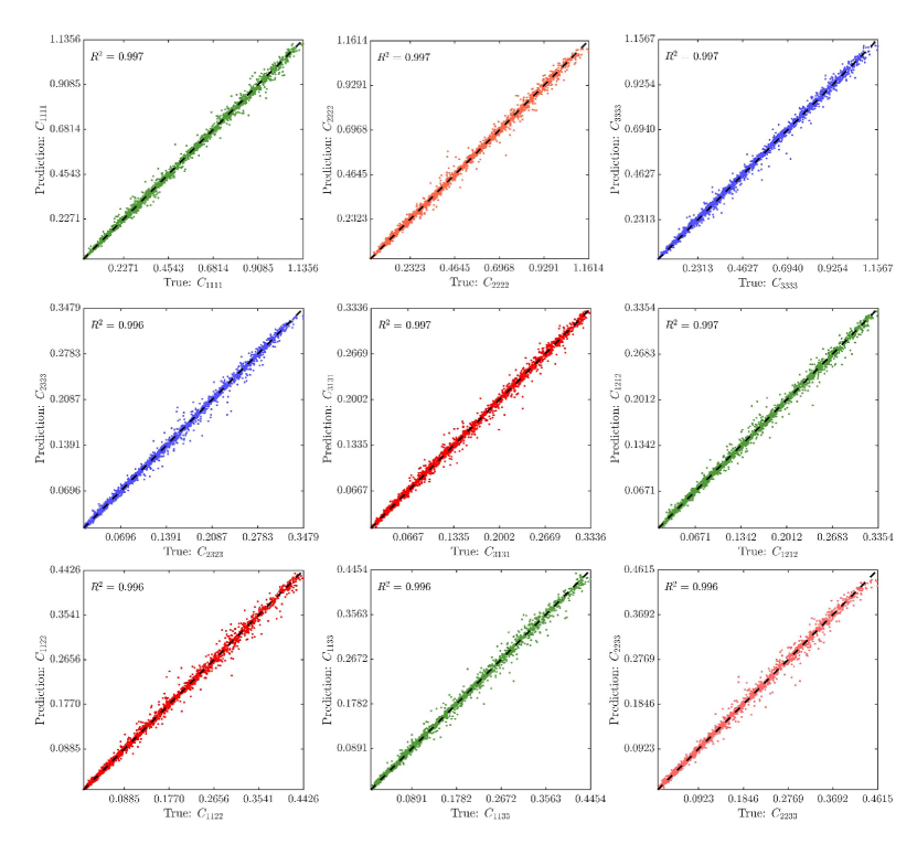
Figure 5: DNN-predicted vs. true components of $\hat{\mathbb{C}}$ in the test dataset. Dashed lines represent the ideal line with zero-intercept and unit-slope; the corresponding $R^{2}$-deviations are indicated.

5 Results

5.1 Performance validation of the surrogate model

Before applying the trained surrogate model for the homogenized stiffness to topology optimization problems, we first assess the accuracy of the surrogate model. For a quantitative assessment, the DNN is trained on $n_{\text{train}}=$19,170 pairs of design parameters and their corresponding effective elastic stiffnesses from FEM, i.e., $(\bm{\Theta},\bm{S})$, followed by testing on an independent test set of containing $n_{\text{test}}=$2,130 pairs. Ideally, the stiffness prediction $\mathcal{F}_{\omega}[\bm{\Theta}]$ from the DNN should agree with the true stiffness, i.e., $\mathcal{F}_{\omega}[\bm{\Theta}]\approx\bm{S}$. Thus, in a plot of predicted vs. true stiffness (Figure 5), the predictions are expected to lie on a line with zero-intercept and unit-slope. The trained DNN achieves an $R^{2}\geq 0.996$ accuracy for each stiffness component. We also perform a similar assessment (Figure 6) for the stiffness sensitivities $\mathcal{F}_{\omega}^{\prime}[\bm{\Theta}]$, where we use the central finite difference scheme applied to FEM-computed stiffnesses to validate the derivatives obtained from the DNN via AD. The AD approach shows good agreement with $R^{2}\geq 0.999$ for each stiffness component.

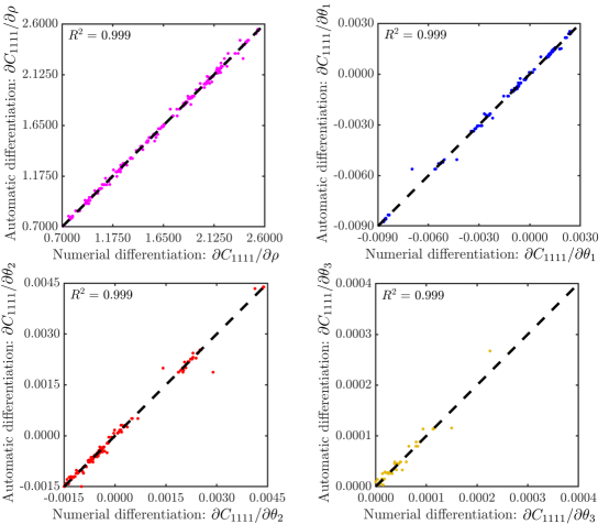
Figure 6: $\mathbb{\hat{C}}_{1111}$ stiffness sensitivity computed via automatic differentiation vs. numerical differentiation in the test set. All dashed lines represent the ideal line with zero-intercept and unit-slope; the corresponding $R^{2}$-deviations are indicated.

5.2 Benchmarks

We investigate three design examples – a cantilever beam, an L-shaped structure, and two designs with simultaneous consideration of multiple load cases. As a baseline, for each example we also present the optimal topologies obtained from the classical SIMP method for a homogeneous and isotropic material with Young’s modulus $E_{s}$ and $\nu_{s}=0.3$ (which are the same values as those of the base material for spinodoids). The penalty factor for SIMP is chosen as $p=4$. To reduce numerical artifacts due to checkerboard patterns, the filter radius $r_{\text{filter}}$ in (15) is set to $0.075$ for all subsequent simulations (thresholding is applied at the end to achieve pure 0-1 solution). For simplicity, we avoid units in the following benchmarks by setting $E_{s}=1$ and normalizing all lengths. To avoid inadmissible design parameters, we choose $\lambda_{1}=600$ and $\lambda_{2}=60\times(180/\pi)\ \text{rad}^{-1}$ in (17) (see Figure 4). In subsequent examples (with the exception of Benchmark IV), the small thickness of the chosen design domains (relative to all other dimensions) and the symmetry in boundary conditions results in uniform distributions of the optimal design parameters across the thickness of each design, thus effectively producing 2D topologies on the macroscale with constant thickness.

5.2.1 Benchmark I: Cantilever beam

We consider a cantilever beam (Figure 7(a)) of size $1.5\times 1.0\times 0.1$ discretized by a mesh of linear tetrahedral elements on a $64\times 48\times 2$ uniform grid. The left vertical face of the beam is clamped (i.e., displacements are suppressed in all directions). A single point load of magnitude $2.0\times 10^{-2}$ in the downward direction is applied at the center of the right vertical face. We seek to minimize the compliance subject to an average relative density constraint of $\bar{\rho}=0.5$. As an initial guess, all elements are initialized with spinodoid relative density $\rho=0.5$, anisotropy parameters $(\theta_{1},\theta_{2},\theta_{3})=(15^{\circ},0^{\circ},0^{\circ})$ and orientation $\alpha=0^{\circ}$. The initial design is intentionally chosen to be lamellar-type (with all lamellae normal to length of the beam). Such a design will strongly deform under axial loads (as evident from their low Young’s moduli; see Figure 1(b)) and therefore show a highly compliant behavior.

The optimal design with anisotropic spinodoid architectures is shown in Figure 8. The material distribution (Figure 8(a)) resembles the optimal topology obtained via SIMP (Figure 7(b)), albeit the former is characterized by larger regions with intermediate density. The optimal compliances obtained by the single-scale SIMP design and our multiscale spinodoid design are shown in Figure 7(c). Contrary to the initial guess of a lamellar topology, the final design is dominated by cubic topologies with larger Young’s moduli along the principal directions. Throughout the macroscale body, the spinodoid microstructures are rotated, so that their preferred orientations follow the material distribution (see Figure 8(a) and Figure 8(e)). Figure 9 illustrates the seamlessly spatially-variant spinodoid topology (with fully resolved microstructure), which bypasses the challenge of incompatible microstructures in periodic metamaterials. To avoid the high computational expense of generating a large mesh with fully resolved microstructure, the microscale topology is illustrated for a representative subdomain only.

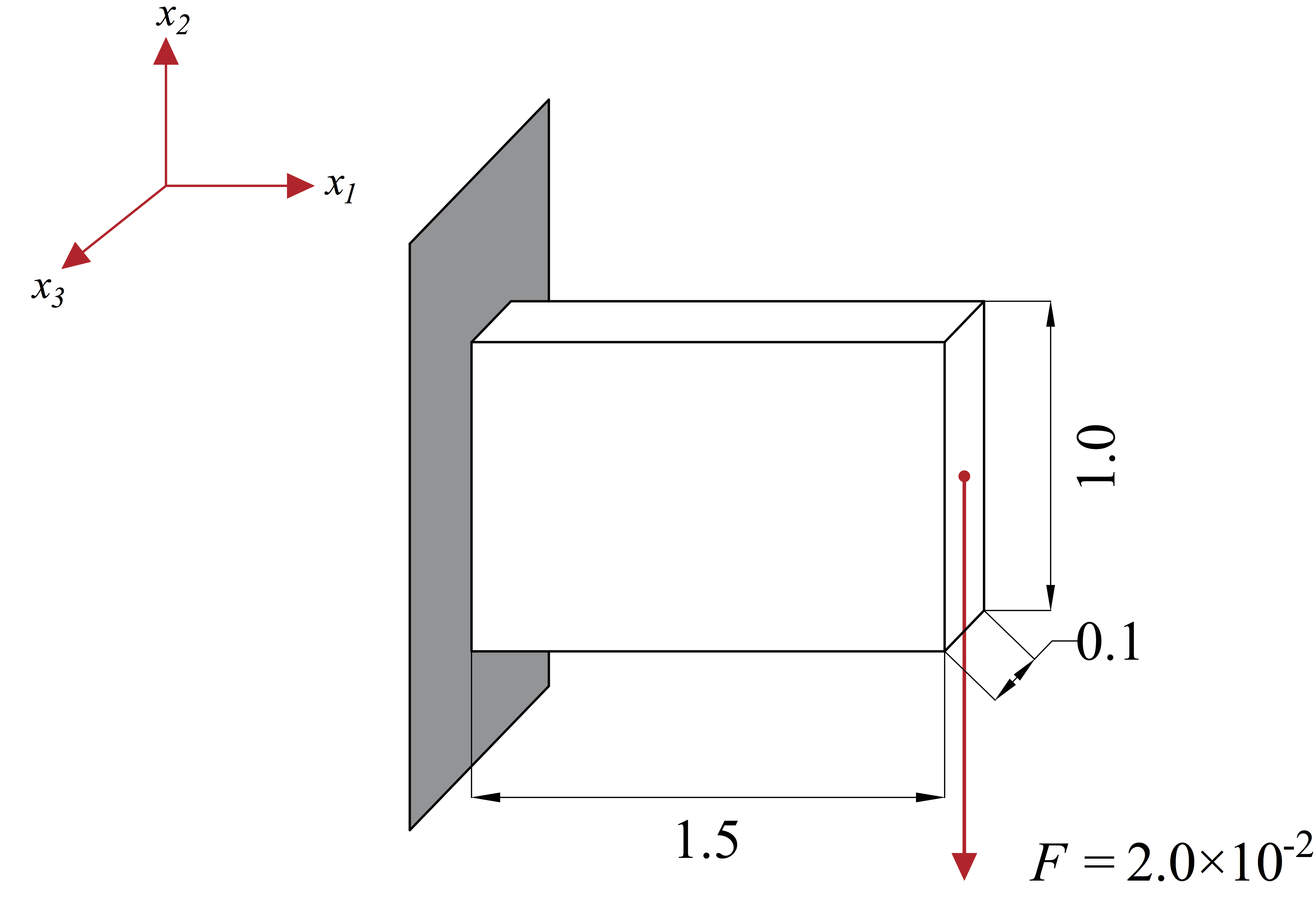
(a)

(b)

	Spinodoid	SIMP
Optimized compliance	$5.602\times 10^{-1}$	${\color[rgb]{0,0,0}5.299\times 10^{-1}}$

(c)

Figure 7: Benchmark I: (a) Schematic of the end-loaded cantilever beam whose compliance is to be optimized. (b) Front view of the optimal topology obtained using the SIMP method. (c) Comparison of the optimal compliance for the spinodoid architecture on the microscale (via proposed method) and a solid material (via SIMP).

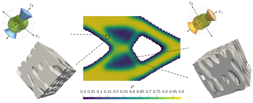
(a) Optimized relative density $\rho$

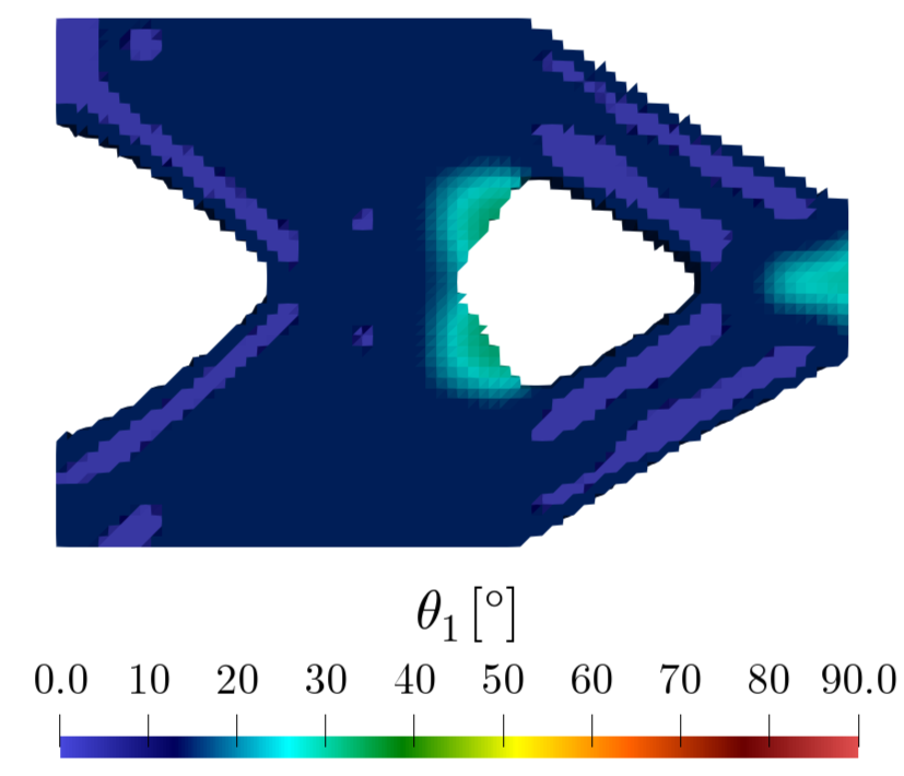
(b) Optimized spinodoid parameter $\theta_{1}$

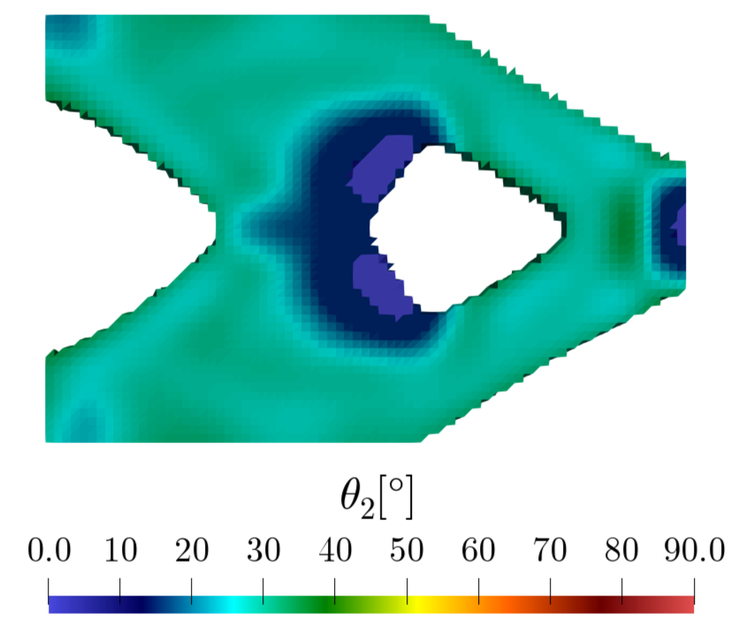
(c) Optimized spinodoid parameter $\theta_{2}$

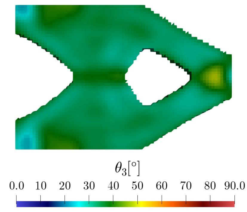
(d) Optimized spinodoid parameter $\theta_{3}$

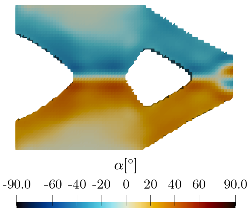
(e) Optimized material orientation $\alpha$

Figure 8: Benchmark I: Front view of the optimal topology (material distribution, anisotropy, and orientation) of the cantilever beam with spinodoid microscale architectures. The spatially-varying design parameters are illustrated across the body, and two examples of distinct microscale topologies are shown in (a).

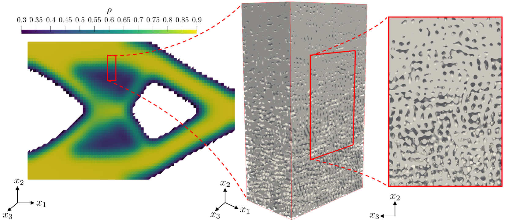
Figure 9: Benchmark I: Seamlessly spatially-variant spinodoid topology with fully resolved microstructure in a subdomain of the optimized cantilever beam design. The microscale GRF is generated with wavenumber $\beta=1600\pi/3$ (arbitrarily chosen and sufficiently large under the assumption of an approximate separation of scales). Details on generating the microscale topology are presented in A.

5.2.2 Benchmark II: L-shaped structure

In this example, an L-shape structure with the dimensions shown in Figure 10(a) is optimized. The top face is fixed in all directions, while a uniformly-distributed vertical load is applied on the lower right edge, as shown. We seek to minimize the total compliance subject to an average relative density constraint of $\bar{\rho}=0.5$. As an initial guess, all elements are initialized with a spinodoid relative density $\rho=0.5$, anisotropy parameters $(\theta_{1},\theta_{2},\theta_{3})=(35^{\circ},15^{\circ},15^{\circ})$ (cubic topology), and orientation $\alpha=0^{\circ}$. The domain is discretized into a finite element mesh with 22,060 linear tetrahedral elements, yielding a total of 110,300 design variables.

The optimal topology with anisotropic spinodoid architectures is shown in Figure 11 and resembles the SIMP result (Figure 10(b)) in terms of the material distribution. The spinodoid-based design achieves $8.35\%$ (Figure 10(c)) improvement in the compliance relative to the SIMP-based design. This is possible due to the spatially-varying anisotropy; e.g., the zoomed-in microstructures in Figure 11(a) show columnar features, which provide high stiffness in the principal stress directions – thus orienting material not only at the macroscale but also on the microscale for optimal compliance. Figure 10(c) lists the optimal compliance for five different mesh resolutions. Increasing the number of finite elements does not affect the optimized compliance significantly. Counter-intuitively, higher mesh resolution may not necessarily yield a lower compliance in the context of a multiply-connected design parameter space and non-convex property space – e.g. for spinodoids, $\rho\in\{0\}\cup[\rho_{\text{min}},1]$ and $\theta_{1},\theta_{2},\theta_{3}\in\{0\}\cup[0,\pi/2]$. Similar observations were reported and explained previously by, e.g., Shiye and Jiejiang (2016) and Kumar et al. (2020b).

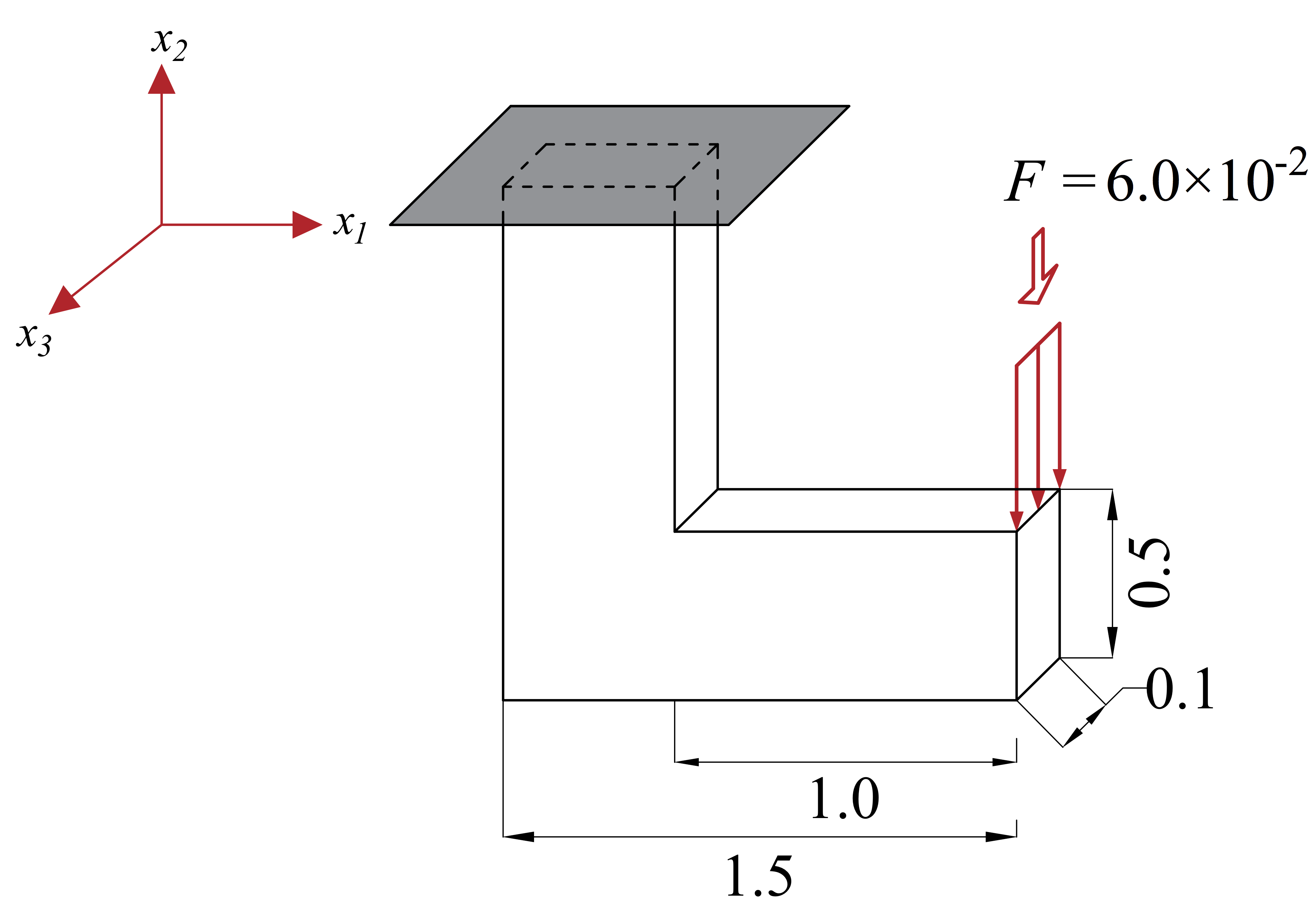
(a)

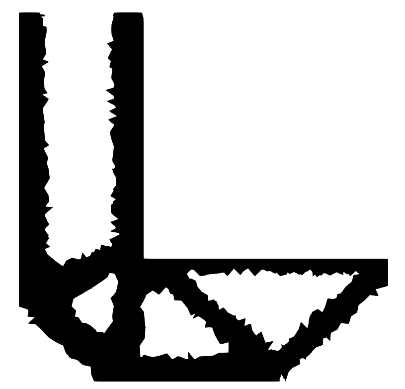
(b)

	Spinodoid						SIMP
No. of elements	6870	8090	14610	22060	26341		22060
Optimized compliance	$2.429\times 10^{1}$	$2.459\times 10^{1}$	$2.425\times 10^{1}$	$2.282\times 10^{1}$	$2.308\times 10^{1}$		$2.490\times 10^{1}$

(c)

Figure 10: Benchmark II: (a) Schematic of the L-shaped structure whose compliance is to be optimized. (b) Front view of the optimal topology obtained using the SIMP method. (c) Comparison of the optimal compliance with spinodoid microscale architecture (via the proposed method for different mesh resolutions) and solid material (via SIMP).

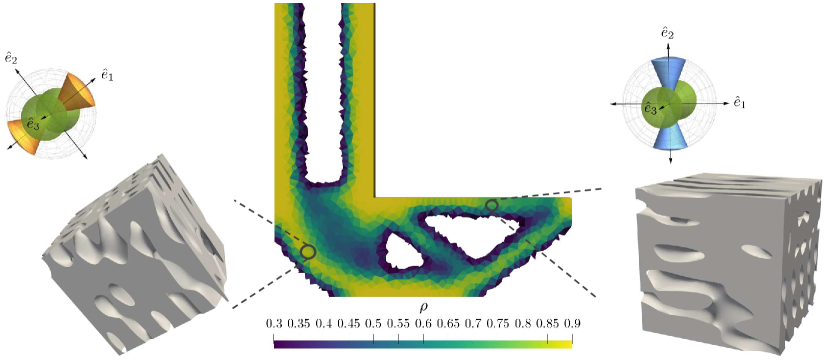
(a) Optimized relative density: $\rho$

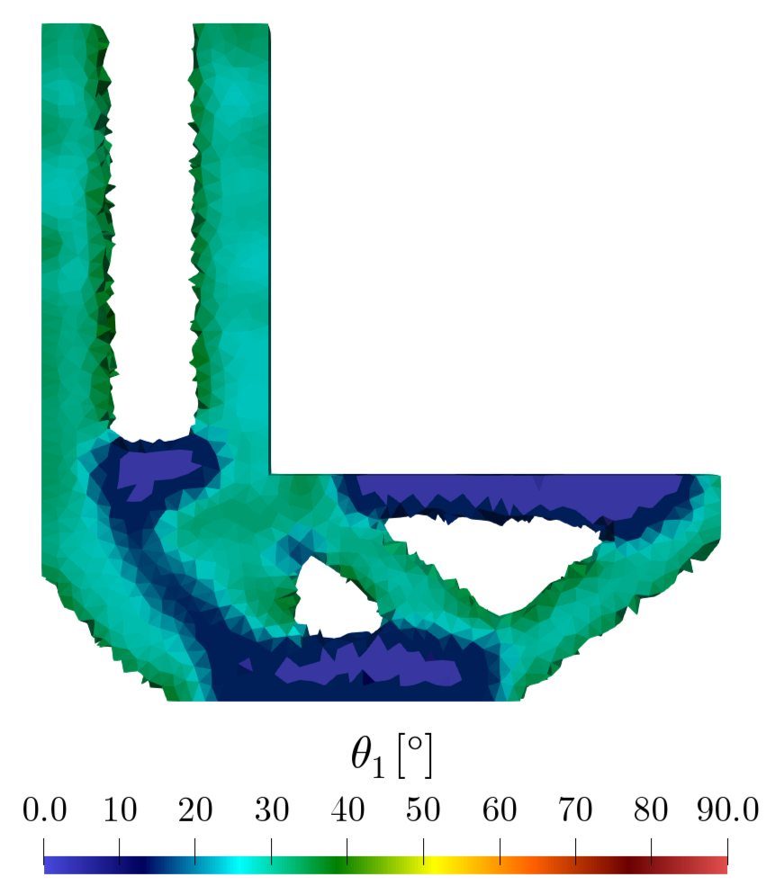
(b) Optimized spinodoid parameter: $\theta_{1}$

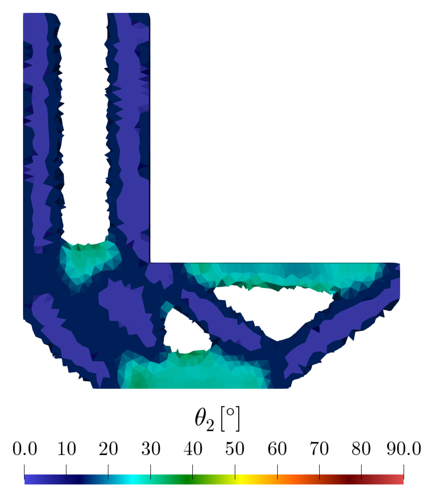
(c) Optimized spinodoid parameter: $\theta_{2}$

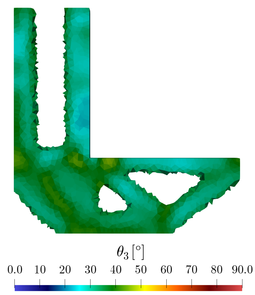
(d) Optimized spinodoid parameter: $\theta_{3}$

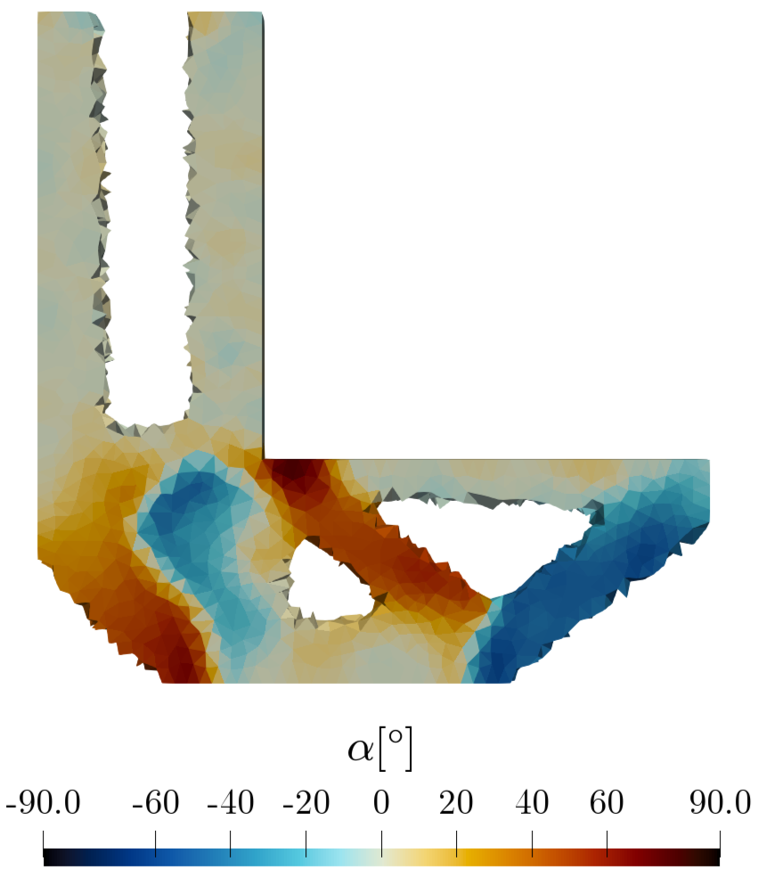
(e) Optimized material orientation: $\alpha$

Figure 11: Benchmark II: Front view of the optimal topology (material distribution, anisotropy, and orientation) of the L-shaped structure with spinodoid microscale architecture. Examples of the spatially-varying design parameters and the corresponding microscale topologies are shown in (a).

5.3 Benchmark III: Multiple load cases – symmetric loading

Here, we extend our multiscale topology optimization algorithm for compliance minimization to the simultaneous consideration of multiple load cases. The objective function in (10) is modified as the sum of the compliances for each individual load case, i.e.,

$$\Phi(x)=\sum^{M}_{i=1}\bm{U}^{i}(x)^{T}\bm{K}^{i}(x)\bm{U}^{i}(x),$$ (23)

where the superscript $(\cdot)^{i}$ denotes the $i^{\text{th}}$ load case, and $M$ is the total number of load cases considered.

As an example, we consider the beam shown in Figure 12(a) with $M=2$ load cases: a uniformly-distributed force in the upward direction on the upper-right edge, and a uniformly-distributed force in the downward direction on the lower-right edge. The average relative density constraint remains $\bar{\rho}=0.5$. As an initial guess, all elements are initialized with a spinodoid relative density $\rho=0.5$, anisotropy parameters $(\theta_{1},\theta_{2},\theta_{3})=(35^{\circ},15^{\circ},15^{\circ})$ (cubic topology), and orientation $\alpha=0^{\circ}$. The domain is discretized into a uniform linear tetrahedral mesh with 25,350 elements and 126,750 design variables .

The optimized design obtained for spinodoid microstructures and SIMP are shown in Figures 12 and 12(b), respectively. Similar to previous benchmarks, the former achieves an improvement of $4.88\%$ in compliance (Figure 5.3) over the SIMP-based design due to the spatially-varying material distribution, anisotropy, and orientation on the microscale.

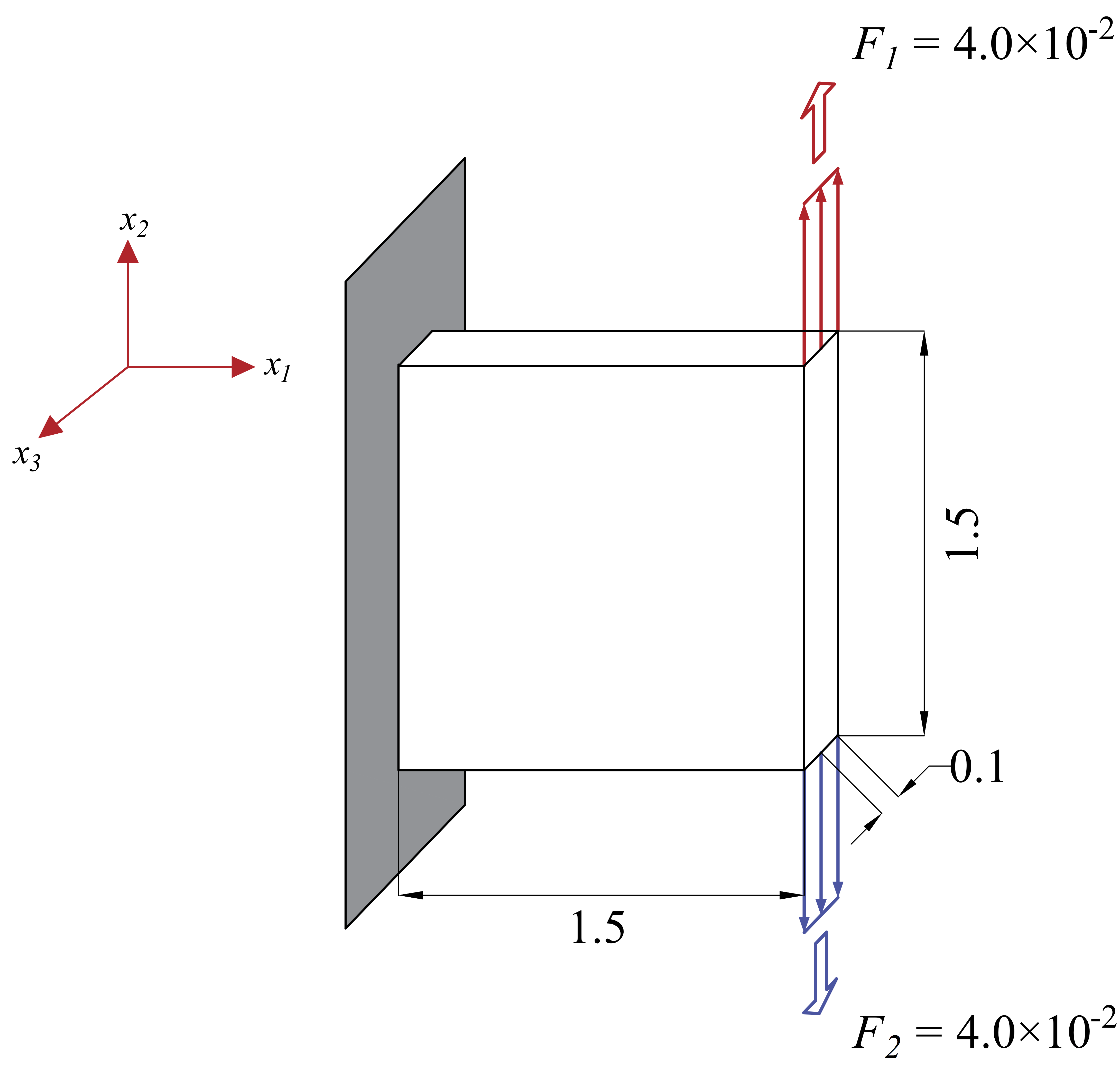
(a)

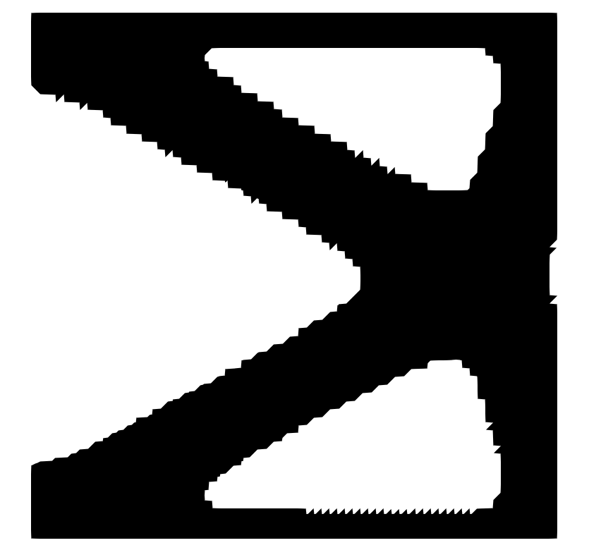
(b)

	Spinodoid						SIMP
No. of elements	12150	16224	21600	25350	31104		25350
Optimized compliance	$8.101\times 10^{1}$	$8.412\times 10^{1}$	$8.340\times 10^{1}$	$8.297\times 10^{1}$	$8.282\times 10^{1}$		$8.723\times 10^{1}$

(c)

(d) Benchmark III: (a) Schematic of the structure to be optimized for two symmetric load cases (shown by the two sets of applied forces). (b) Front view of the optimal topology obtained using the SIMP method. (c) Comparison of the optimal compliance with spinodoid microscale architectures (via the proposed method for different mesh resolutions) and solid material (via SIMP).

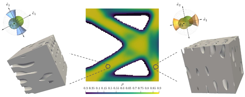
(e) Optimized relative density $\rho$

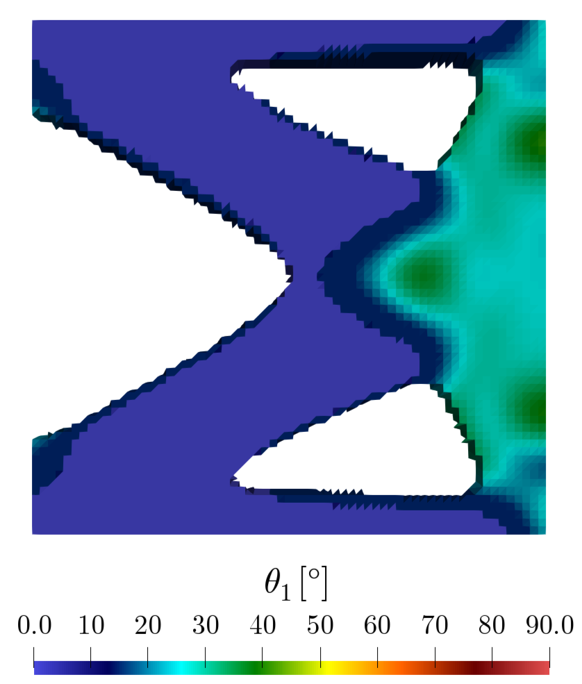
(f) Optimized spinodoid parameter $\theta_{1}$

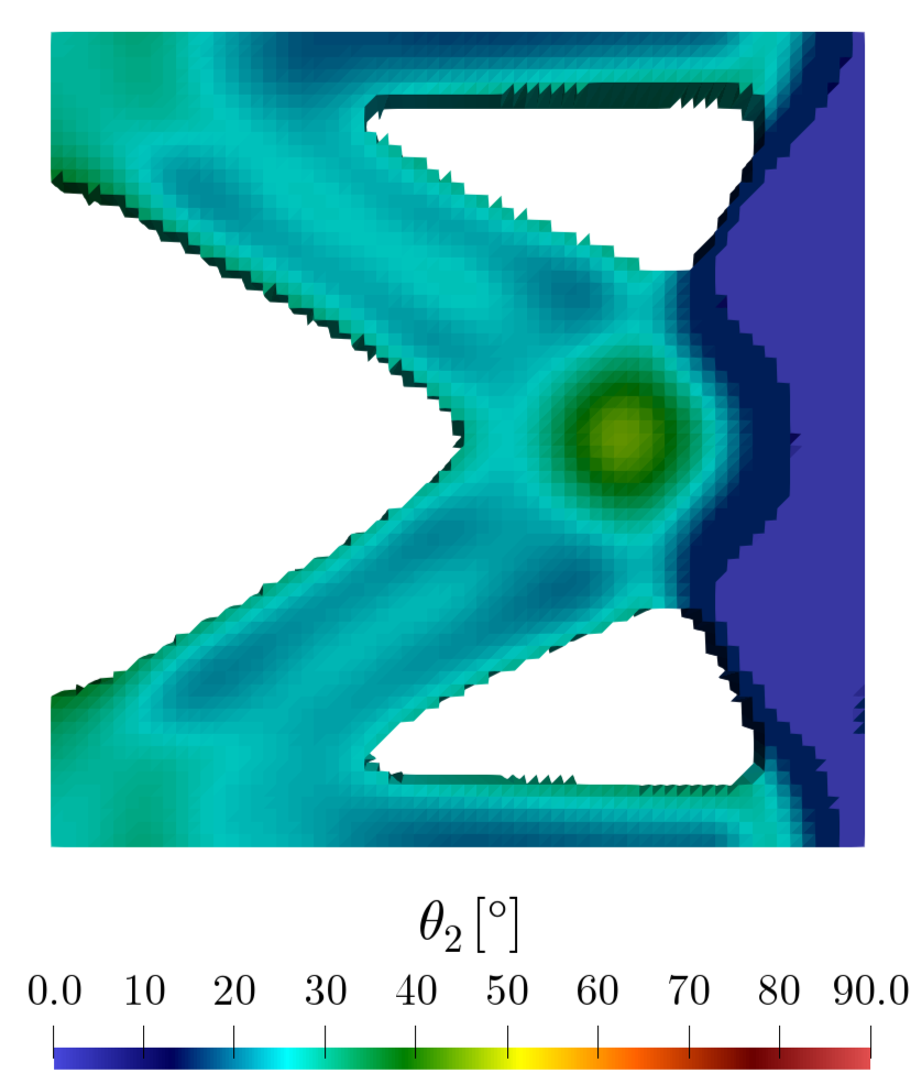
(g) Optimized spinodoid parameter $\theta_{2}$

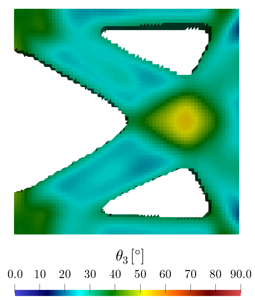
(h) Optimized spinodoid parameter $\theta_{3}$

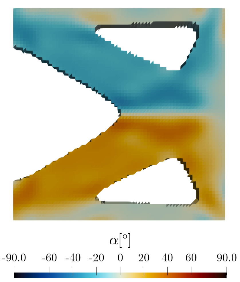
(i) Optimized material orientation $\alpha$

Figure 12: Benchmark III: Front view of the optimal topology (material distribution, anisotropy, and orientation) of the spinodoid-based structure, optimized for two symmetric load cases. Examples of the spatially-varying design parameters and the corresponding microscale topologies are shown in (a).

5.4 Benchmark IV: Multiple load cases – non-symmetric loading

We modify Benchmark III (Section 5.3) by considering the three non-symmetric load cases shown in Figure 13(a), which involve three point loads of the same magnitude but at three different corners ($M=3$). An average volume constraint of $\bar{\rho}=0.4$ is imposed. The domain is discretized into a uniform linear tetrahedral mesh with 48,000 elements and 240,000 design variables.

Optimal SIMP- as well as spinodoid-based designs are illustrated in Figures 13(b) as well as in Figures 14 and 15, respectively. Compared with the previous benchmarks, the spinodoid-based design shows only minor improvement (1.27%) in compliance over SIMP (Figure 13(c)). This can, in fact, be expected for the simultaneous optimization for multiple load cases applied in different directions, since – under such constraints – the structure is likely to favor isotropic topologies as the best compromise between all design cases, thus leading to similar performance as SIMP. We note that the small improvement of 1.27% in compliance further needs to be considered with caution, as it can partially be due to numerical artifacts.

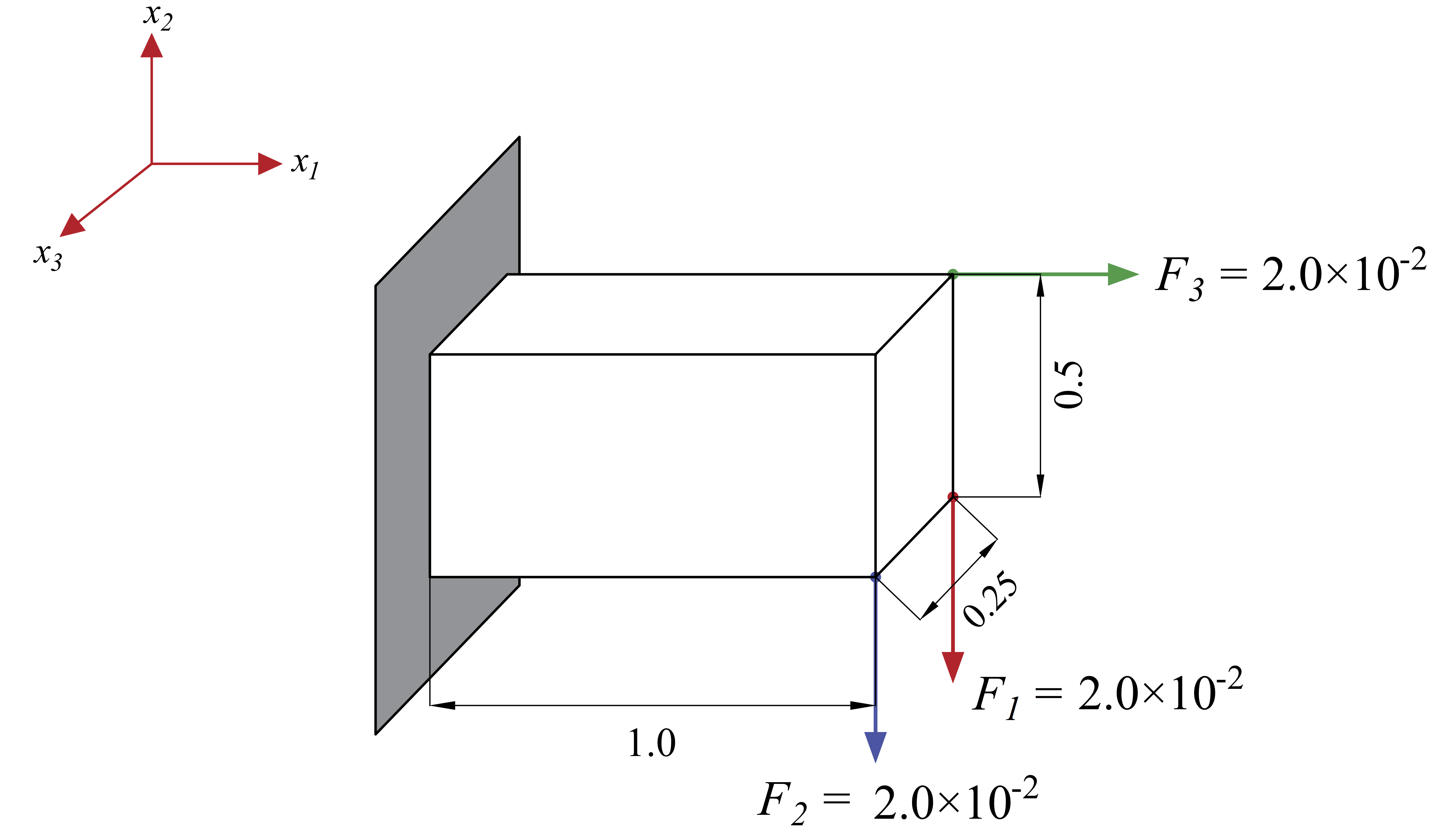
(a)

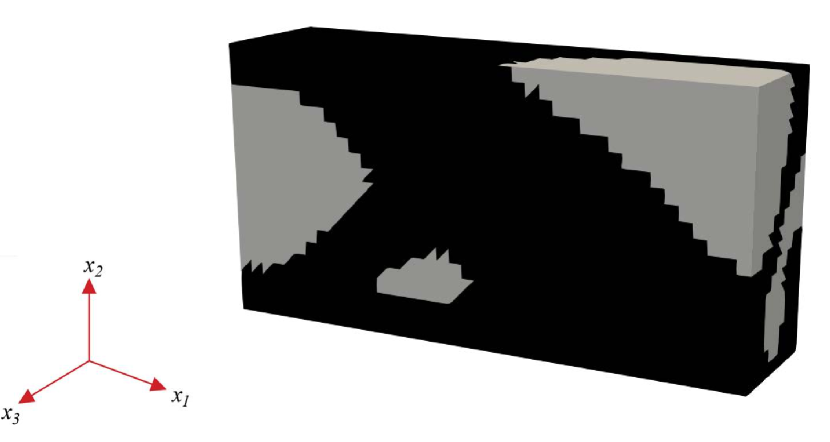
(b)

	Spinodoid	SIMP
Optimized compliance	$7.8\times 10^{3}$	$7.9\times 10^{3}$

(c)

Figure 13: Benchmark IV: (a) Schematic of the structure to be optimized for three non-symmetric load cases. (b) 3D view of the optimal topology obtained using the SIMP method. Gray regions here denote complete void. (c) Comparison of the optimal compliance with spinodoid microscale architecture (via the proposed method) and solid material (via SIMP).

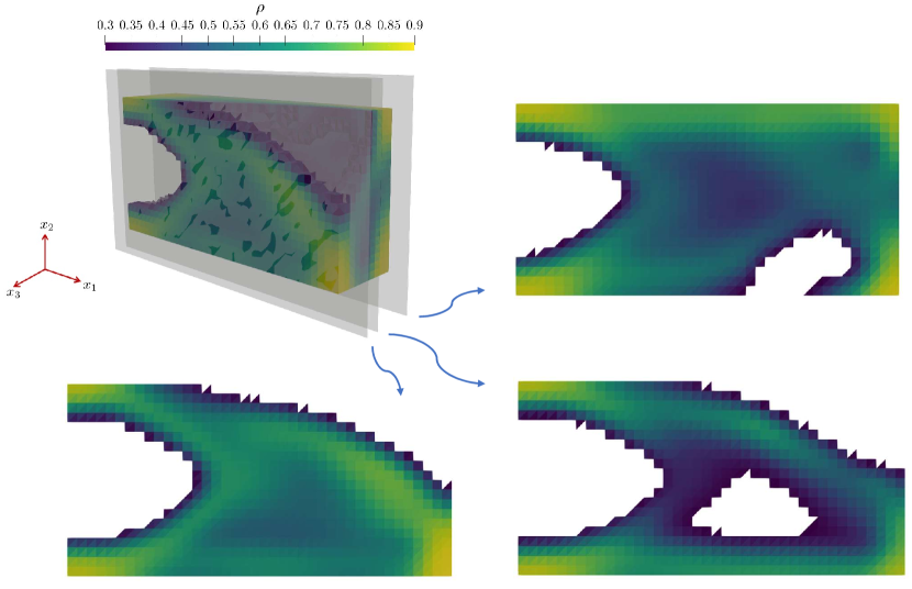
Figure 14: Benchmark IV: Optimal material distribution in the spinodoid-based structure with multiple non-symmetric load cases. Front-view of multiple cross-sectional planes are shown here.

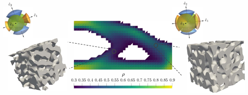
(a) Optimized relative density: $\rho$

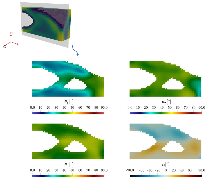
(b) Optimized spinodoid parameter: $\theta_{1},\theta_{2},\theta_{3},\alpha$

Figure 15: Benchmark IV: Optimal topology (material distribution, anisotropy, and orientation) of the spinodoid-based structure optimized for three non-symmetric load cases. The front view of the cross-section at $x_{3}=0.2$ is shown here. Examples of spatially-varying design parameters and the corresponding microscale topologies are shown in (a).

6 Conclusions

We have presented a two-scale topology optimization framework for macroscopic bodies made of a spatially-variant microscale architecture based on spinodoid topologies. Inspired by microstructures produced by spinodal decomposition, the spinodoid topologies are anisotropic and described by a set of four design parameters (the relative density and the orientation distribution of wave vectors in the underlying Gaussian random field). The topology optimization problem minimizes the linear elastic compliance of macroscopic bodies by solving both for the displacement field and for a continuous field of the design parameters. The effective material response at any point on the macroscale is identified with the homogenized, effective response of a representative volume element filled by the spinodoid topology defined by the local design parameters. To bypass costly computational homogenization simulations, we here introduce a new approach based on a deep neural network as a surrogate model that maps the design parameters onto the effective fourth-order stiffness tensor. Aside from significantly speeding up calculations, this approach also provides exact sensitivities (required for gradient-based optimization) at low numerical costs. . We presented four benchmarks of linear elastic compliance optimization for different macroscopic bodies experiencing single and multiple load cases, which demonstrate the applicability of the framework and highlight advantages over, e.g., the classical SIMP approach due to the enlarged design space available by optimizing both macro- and microscales. Although our study was specific to spinodoid architectures and simple macroscale boundary value problems, the presented approach is sufficiently general to extend to other microscale architectures and more complex boundary value problems.

Appendix A Generating a spatially-variant spinodoid topology with fully resolved microstructure

The nonlinear optimization problem (11) yields the set of spatially-variant design parameters $\mathcal{X}=\{\bm{\chi}^{e},e=1,\dots,n\}$ at the quadrature points $\{\bm{x}^{e},e=1,\dots,n\}$ of the macroscale finite element mesh. To generate the fully resolved spinodoid microstructure of the optimized macroscale body, we must turn that quadrature-point information into a seamless spinodoid architecture across the macroscale body $\Omega$. Here, we consider a weighted superposition of multiple GRFs, each described by its design parameters in $\mathcal{X}$. Let $q(\bm{x},\bm{x}^{e})$ be a Gaussian weight function defined by

$$q(\bm{x},\bm{x}^{e})=\frac{\exp(-\kappa\|\bm{x}-\bm{x}^{e}\|^{2})}{Z(\bm{x})}$$ (24)

with a length scale parameter $\kappa>0$ and

$$Z(\bm{x})=\sum_{e=1}^{n}\exp(-\kappa\|\bm{x}-\bm{x}^{e}\|^{2})$$ (25)

ensuring partition of unity, i.e., $\sum_{e=1}^{n}q(\bm{x},\bm{x}^{e})=1$. Let $\varphi^{e}(\bm{x})$ denote the GRF described by the design parameters $\bm{\chi}^{e}=(\rho^{e},\theta_{1}^{e},\theta_{2}^{e},\theta_{3}^{e},\alpha^{e})^{\text{T}}$ and the corresponding level set

$$\varphi_{0}^{e}=\sqrt{2}\text{erf}^{-1}(2\rho^{e}-1).$$ (26)

When considering a total of $n$ quadrature points, we define an interpolated GRF

$$\bar{\varphi}(\bm{x})=\sum_{e=1}^{n}q(\bm{x},\bm{x}^{e})(\varphi^{e}(\bm{x})-\varphi^{e}_{0})$$ (27)

with the global level set (for all points $\bm{x}\in\Omega$)

$$\bar{\xi}(\bm{x})=\begin{cases}1\text{ (solid)}&\quad\text{if }\quad\bar{\varphi}(\bm{x})\leq 0,\\ 0\text{ (void)}&\quad\text{if }\quad\bar{\varphi}(\bm{x})>0.\end{cases}$$ (28)

For a given point $\bm{x}\in\Omega$ in the proximity of $\bm{x}^{e}$, the exponential decay in $q(\bm{x},\cdot)$ (for sufficiently large $\kappa$) ensures that $q(\bm{x},\bm{x}^{e})\approx 1$ and $\bar{\varphi}(\bm{x})\approx\varphi^{e}(\bm{x})$ with level set $\varphi^{e}_{0}$; i.e., the interpolated GRF approximates the individual GRF described by $\bm{\chi}^{e}$. Elsewhere, the above yields a superposition of those GRFs of nearby quadrature points to generate a seamlessly varying spinodoid topology throughout the entire domain $\Omega$. The computational efficiency of the interpolation can be improved by reducing the summation in (27) to only those terms with $q(\bm{x},\cdot)$ greater than a minimum cut-off value. We point out that the GRF wave number $\beta$ must be sufficiently large to ensure an effective separation of scales between the micro- and macroscales.

In order to spatially resolve the microstructure over $\Omega$, $\bm{x}$ can conveniently be sampled from a separate mesh with significantly higher resolution than the mesh used for FEM (thus keeping the FEM costs low but providing high-resolution architectures for visualization and part production). Note that we here do not consider fabrication constraints nor specifics of additive manufacturing.

Appendix B

Task	Software	Parallelization & Hardware	Runtime
Stiffness computation using FEM	In-house C++ FEM code	16 MPI cores§	5 minutes
Stiffness computation via the DNN†	PyTorch in Python	CPU, no parallelization⋆	0.001 seconds
Training the DNN	PyTorch in Python	CPU, no parallelization⋆	10 minutes
Benchmark I	Python	CPU, no parallelization§	3 hours
Benchmark II	Python	CPU, no parallelization§	3.5 hours
Benchmark III	Python	CPU, no parallelization§	4.5 hours
Benchmark IV	Python	CPU, no parallelization§	8 hours

Table 1:

References

- Adler and Taylor (2007) Adler, R.J., Taylor, J.E., 2007. Random Fields and Geometry. Springer-Verlag New York.
- Al-Ketan and Abu Al-Rub (2019) Al-Ketan, O., Abu Al-Rub, R.K., 2019. Multifunctional mechanical metamaterials based on triply periodic minimal surface lattices. Advanced Engineering Materials 0, 1900524. URL: https://www.onlinelibrary.wiley.com/doi/abs/10.1002/adem.201900524, doi:10.1002/adem.201900524, arXiv:https://www.onlinelibrary.wiley.com/doi/pdf/10.1002/adem.201900524.
- Allen (2001) Allen, S., 2001. Spinodal decomposition, in: Buschow, K.J., Cahn, R.W., Flemings, M.C., Ilschner, B., Kramer, E.J., Mahajan, S., Veyssière, P. (Eds.), Encyclopedia of Materials: Science and Technology. Elsevier, Oxford, pp. 8761 – 8764. URL: http://www.sciencedirect.com/science/article/pii/B0080431526015692, doi:https://doi.org/10.1016/B0-08-043152-6/01569-2.
- Banga et al. (2018) Banga, S., Gehani, H., Bhilare, S., Patel, S., Kara, L., 2018. 3d topology optimization using convolutional neural networks. arXiv preprint arXiv:1808.07440 .
- Barthelemy and Hall (1995) Barthelemy, J.F., Hall, L.E., 1995. Automatic differentiation as a tool in engineering design. Structural optimization 9, 76–82.
- Bendsøe (1989) Bendsøe, M.P., 1989. Optimal shape design as a material distribution problem. Structural optimization 1, 193–202.
- Bendsoe and Kikuchi (1988) Bendsoe, M.P., Kikuchi, N., 1988. Generating optimal topologies in structural design using a homogenization method. Computer Methods in Applied Mechanics and Engineering 71, 197 – 224. URL: http://www.sciencedirect.com/science/article/pii/0045782588900862, doi:https://doi.org/10.1016/0045-7825(88)90086-2.
- Bendsøe and Sigmund (1999) Bendsøe, M.P., Sigmund, O., 1999. Material interpolation schemes in topology optimization. Archive of applied mechanics 69, 635–654.
- Bendsoe and Sigmund (2013) Bendsoe, M.P., Sigmund, O., 2013. Topology optimization: theory, methods, and applications. Springer Science & Business Media.
- Berger et al. (2017) Berger, J., Wadley, H., McMeeking, R., 2017. Mechanical metamaterials at the theoretical limit of isotropic elastic stiffness. Nature 543, 533–537.
- Bruder and Brenn (1992) Bruder, F., Brenn, R., 1992. Spinodal decomposition in thin films of a polymer blend. Physical review letters 69, 624.
- Bruns and Tortorelli (2001) Bruns, T.E., Tortorelli, D.A., 2001. Topology optimization of non-linear elastic structures and compliant mechanisms. Computer methods in applied mechanics and engineering 190, 3443–3459.
- Cahn (1961) Cahn, J.W., 1961. On spinodal decomposition. Acta metallurgica 9, 795–801.
- Cahn (1965) Cahn, J.W., 1965. Phase separation by spinodal decomposition in isotropic systems. The Journal of Chemical Physics 42, 93–99.
- Cahn and Hilliard (1958) Cahn, J.W., Hilliard, J.E., 1958. Free energy of a nonuniform system. i. interfacial free energy. The Journal of chemical physics 28, 258–267.
- Charpentier (2012) Charpentier, I., 2012. On higher-order differentiation in nonlinear mechanics. Optimization Methods and Software 27, 221–232.
- Coelho et al. (2008) Coelho, P., Fernandes, P., Guedes, J., Rodrigues, H., 2008. A hierarchical model for concurrent material and topology optimisation of three-dimensional structures. Structural and Multidisciplinary Optimization 35, 107–115.
- Cook (1970) Cook, H.E., 1970. Brownian motion in spinodal decomposition. Acta Metallurgica 18, 297–306.
- Cook et al. (2001) Cook, R.D., Malkus, D.S., Plesha, M.E., Witt, R.J., 2001. Concepts and Applications of Finite Element Analysis, 4th Edition. 4 ed., Wiley.
- Diaz and Bendsøe (1992) Diaz, A., Bendsøe, M., 1992. Shape optimization of structures for multiple loading conditions using a homogenization method. Structural optimization 4, 17–22.
- Erlebacher et al. (2001) Erlebacher, J., Aziz, M.J., Karma, A., Dimitrov, N., Sieradzki, K., 2001. Evolution of nanoporosity in dealloying. Nature 410, 450–453.
- Evans et al. (2010) Evans, A.G., He, M., Deshpande, V.S., Hutchinson, J.W., Jacobsen, A.J., Carter, W.B., 2010. Concepts for enhanced energy absorption using hollow micro-lattices. International Journal of Impact Engineering 37, 947–959.
- Gao et al. (2019) Gao, J., Luo, Z., Li, H., Gao, L., 2019. Topology optimization for multiscale design of porous composites with multi-domain microstructures. Computer Methods in Applied Mechanics and Engineering 344, 451–476.
- Gao et al. (2012) Gao, T., Zhang, W., Duysinx, P., 2012. A bi-value coding parameterization scheme for the discrete optimal orientation design of the composite laminate. International Journal for Numerical Methods in Engineering 91, 98–114.
- Gibiansky and Cherkaev (2018) Gibiansky, L., Cherkaev, A.V., 2018. Microstructures of composites of extremal rigidity and exact bounds on the associated energy density, in: Topics in the mathematical modelling of composite materials. Springer, pp. 273–317.
- Gibson et al. (2010) Gibson, L.J., Ashby, M.F., Harley, B.A., 2010. Cellular materials in nature and medicine. Cambridge University Press.
- Griewank and Walther (2008) Griewank, A., Walther, A., 2008. Evaluating derivatives: principles and techniques of algorithmic differentiation. volume 105. Siam.
- Groen et al. (2019) Groen, J.P., Wu, J., Sigmund, O., 2019. Homogenization-based stiffness optimization and projection of 2d coated structures with orthotropic infill. Computer Methods in Applied Mechanics and Engineering 349, 722–742. URL: http://www.sciencedirect.com/science/article/pii/S0045782519301021, doi:10.1016/j.cma.2019.02.031.
- Guell Izard et al. (2019) Guell Izard, A., Bauer, J., Crook, C., Turlo, V., Valdevit, L., 2019. Ultrahigh energy absorption multifunctional spinodal nanoarchitectures. Small 15, 1903834. URL: https://onlinelibrary.wiley.com/doi/abs/10.1002/smll.201903834, doi:https://doi.org/10.1002/smll.201903834, arXiv:https://onlinelibrary.wiley.com/doi/pdf/10.1002/smll.201903834.
- Han et al. (2017) Han, S.C., Choi, J.M., Liu, G., Kang, K., 2017. A microscopic shell structure with Schwarz’s D-Surface. Scientific Reports 7, 13405. URL: https://doi.org/10.1038/s41598-017-13618-3, doi:10.1038/s41598-017-13618-3.
- Hodge et al. (2007) Hodge, A., Biener, J., Hayes, J., Bythrow, P., Volkert, C., Hamza, A., 2007. Scaling equation for yield strength of nanoporous open-cell foams. Acta Materialia 55, 1343–1349.
- Hsieh et al. (2019) Hsieh, M.T., Endo, B., Zhang, Y., Bauer, J., Valdevit, L., 2019. The mechanical response of cellular materials with spinodal topologies. Journal of the Mechanics and Physics of Solids 125, 401–419.
- Huet (1990) Huet, C., 1990. Application of variational concepts to size effects in elastic heterogeneous bodies. Journal of the Mechanics and Physics of Solids 38, 813–841.
- Jiang et al. (2019) Jiang, D., Hoglund, R., Smith, D., 2019. Continuous fiber angle topology optimization for polymer composite deposition additive manufacturing applications. Fibers 7, 14. doi:10.3390/fib7020014.
- Kingma and Ba (2014) Kingma, D.P., Ba, J., 2014. Adam: A method for stochastic optimization. arXiv preprint arXiv:1412.6980 .
- Kumar et al. (2020a) Kumar, S., Tan, S., Zheng, L., Kochmann, D.M., 2020a. Inverse-designed spinodoid metamaterials. npj Computational Materials 6, 73. URL: https://doi.org/10.1038/s41524-020-0341-6, doi:10.1038/s41524-020-0341-6.
- Kumar et al. (2020b) Kumar, S., Vidyasagar, A., Kochmann, D.M., 2020b. An assessment of numerical techniques to find energy-minimizing microstructures associated with nonconvex potentials. International Journal for Numerical Methods in Engineering 121, 1595–1628. URL: https://onlinelibrary.wiley.com/doi/abs/10.1002/nme.6280, doi:10.1002/nme.6280, arXiv:https://onlinelibrary.wiley.com/doi/pdf/10.1002/nme.6280.
- Latture et al. (2018) Latture, R.M., Rodriguez, R.X., Holmes, L.R., Zok, F.W., 2018. Effects of nodal fillets and external boundaries on compressive response of an octet truss. Acta Materialia 149, 78 – 87. URL: http://www.sciencedirect.com/science/article/pii/S1359645418300168, doi:https://doi.org/10.1016/j.actamat.2017.12.060.
- Lee et al. (2012) Lee, J.H., Singer, J.P., Thomas, E.L., 2012. Micro-/nanostructured mechanical metamaterials. Advanced materials 24, 4782–4810.
- Lee and Mohraz (2010) Lee, M.N., Mohraz, A., 2010. Bicontinuous macroporous materials from bijel templates. Advanced Materials 22, 4836–4841.
- Lei et al. (2019) Lei, X., Liu, C., Du, Z., Zhang, W., Guo, X., 2019. Machine learning-driven real-time topology optimization under moving morphable component-based framework. Journal of Applied Mechanics 86.
- Mateos et al. (2019) Mateos, A.J., Huang, W., Zhang, Y.W., Greer, J.R., 2019. Discrete-continuum duality of architected materials: Failure, flaws, and fracture. Advanced Functional Materials 29, 1806772. URL: https://onlinelibrary.wiley.com/doi/abs/10.1002/adfm.201806772, doi:10.1002/adfm.201806772, arXiv:https://onlinelibrary.wiley.com/doi/pdf/10.1002/adfm.201806772.
- Meza et al. (2014) Meza, L.R., Das, S., Greer, J.R., 2014. Strong, lightweight, and recoverable three-dimensional ceramic nanolattices. Science 345, 1322–1326. URL: https://science.sciencemag.org/content/345/6202/1322, doi:10.1126/science.1255908, arXiv:https://science.sciencemag.org/content/345/6202/1322.full.pdf.
- Meza et al. (2017) Meza, L.R., Phlipot, G.P., Portela, C.M., Maggi, A., Montemayor, L.C., Comella, A., Kochmann, D.M., Greer, J.R., 2017. Reexamining the mechanical property space of three-dimensional lattice architectures. Acta Materialia 140, 424 – 432. URL: http://www.sciencedirect.com/science/article/pii/S1359645417307073, doi:https://doi.org/10.1016/j.actamat.2017.08.052.
- Nguyen et al. (2017) Nguyen, B.D., Han, S.C., Jung, Y.C., Kang, K., 2017. Design of the p-surfaced shellular, an ultra-low density material with micro-architecture. Computational Materials Science 139, 162 – 178. URL: http://www.sciencedirect.com/science/article/pii/S0927025617303865, doi:https://doi.org/10.1016/j.commatsci.2017.07.025.
- Nguyen et al. (2010) Nguyen, T.H., Paulino, G.H., Song, J., Le, C.H., 2010. A computational paradigm for multiresolution topology optimization (mtop). Structural and Multidisciplinary Optimization 41, 525–539. URL: https://doi.org/10.1007/s00158-009-0443-8, doi:10.1007/s00158-009-0443-8.
- Nomura et al. (2015) Nomura, T., Dede, E.M., Lee, J., Yamasaki, S., Matsumori, T., Kawamoto, A., Kikuchi, N., 2015. General topology optimization method with continuous and discrete orientation design using isoparametric projection. International Journal for Numerical Methods in Engineering 101, 571–605.
- Pedersen (1989) Pedersen, P., 1989. On optimal orientation of orthotropic materials. Structural optimization 1, 101–106.
- Pedersen (1990) Pedersen, P., 1990. Bounds on elastic energy in solids of orthotropic materials. Structural optimization 2, 55–63.
- Pedersen (1991) Pedersen, P., 1991. On thickness and orientational design with orthotropic materials. Structural Optimization 3, 69–78.
- Portela et al. (2018) Portela, C.M., Greer, J.R., Kochmann, D.M., 2018. Impact of node geometry on the effective stiffness of non-slender three-dimensional truss lattice architectures. Extreme Mechanics Letters 22, 138 – 148. URL: http://www.sciencedirect.com/science/article/pii/S2352431618300725, doi:https://doi.org/10.1016/j.eml.2018.06.004.
- Portela et al. (2020) Portela, C.M., Vidyasagar, A., Krödel, S., Weissenbach, T., Yee, D.W., Greer, J.R., Kochmann, D.M., 2020. Extreme mechanical resilience of self-assembled nanolabyrinthine materials. Proceedings of the National Academy of Sciences 117, 5686–5693.
- Rodrigues et al. (2002) Rodrigues, H., Guedes, J.M., Bendsoe, M., 2002. Hierarchical optimization of material and structure. Structural and Multidisciplinary Optimization 24, 1–10.
- Salvalaglio et al. (2015) Salvalaglio, M., Backofen, R., Bergamaschini, R., Montalenti, F., Voigt, A., 2015. Faceting of equilibrium and metastable nanostructures: a phase-field model of surface diffusion tackling realistic shapes. Crystal Growth & Design 15, 2787–2794.
- Schumacher et al. (2015) Schumacher, C., Bickel, B., Rys, J., Marschner, S., Daraio, C., Gross, M., 2015. Microstructures to control elasticity in 3d printing. ACM Trans. Graph. 34.
- Schury et al. (2012) Schury, F., Stingl, M., Wein, F., 2012. Efficient two-scale optimization of manufacturable graded structures. SIAM Journal on Scientific Computing 34, B711–B733.
- Setoodeh et al. (2005) Setoodeh, S., Abdalla, M.M., Gürdal, Z., 2005. Combined topology and fiber path design of composite layers using cellular automata. Structural and Multidisciplinary Optimization 30, 413–421.
- Shiye and Jiejiang (2016) Shiye, B., Jiejiang, Z., 2016. Topology optimization design of 3d continuum structure with reserved hole based on variable density method. Journal of Engineering Science and Technology Review 9, 121–128. doi:10.25103/jestr.092.20.
- Sigmund (1994) Sigmund, O., 1994. Materials with prescribed constitutive parameters: an inverse homogenization problem. International Journal of Solids and Structures 31, 2313–2329.
- Sigmund (1995) Sigmund, O., 1995. Tailoring materials with prescribed elastic properties. Mechanics of Materials 20, 351–368.
- Sigmund (1997) Sigmund, O., 1997. On the design of compliant mechanisms using topology optimization. Journal of Structural Mechanics 25, 493–524.
- Sigmund (2001) Sigmund, O., 2001. A 99 line topology optimization code written in matlab. Structural and multidisciplinary optimization 21, 120–127.
- Sigmund (2007) Sigmund, O., 2007. Morphology-based black and white filters for topology optimization. Structural and Multidisciplinary Optimization 33, 401–424.
- Sigmund and Maute (2013) Sigmund, O., Maute, K., 2013. Topology optimization approaches. Structural and Multidisciplinary Optimization 48, 1031–1055.
- Sigmund and Petersson (1998) Sigmund, O., Petersson, J., 1998. Numerical instabilities in topology optimization: a survey on procedures dealing with checkerboards, mesh-dependencies and local minima. Structural optimization 16, 68–75.
- Sivapuram et al. (2016) Sivapuram, R., Dunning, P.D., Kim, H.A., 2016. Simultaneous material and structural optimization by multiscale topology optimization. Structural and multidisciplinary optimization 54, 1267–1281.
- Sosnovik and Oseledets (2019) Sosnovik, I., Oseledets, I., 2019. Neural networks for topology optimization. Russian Journal of Numerical Analysis and Mathematical Modelling 34, 215–223.
- Soyarslan et al. (2018) Soyarslan, C., Bargmann, S., Pradas, M., Weissmüller, J., 2018. 3d stochastic bicontinuous microstructures: Generation, topology and elasticity. Acta materialia 149, 326–340.
- Stegmann and Lund (2005) Stegmann, J., Lund, E., 2005. Discrete material optimization of general composite shell structures. International Journal for Numerical Methods in Engineering 62, 2009–2027.
- Stewart and Goldenfeld (1992) Stewart, J., Goldenfeld, N., 1992. Spinodal decomposition of a crystal surface. Physical Review A 46, 6505.
- Su and Renaud (1997) Su, J., Renaud, J.E., 1997. Automatic differentiation in robust optimization. AIAA journal 35, 1072–1079.
- Suzuki and Kikuchi (1991) Suzuki, K., Kikuchi, N., 1991. A homogenization method for shape and topology optimization. Computer Methods in Applied Mechanics and Engineering 93, 291 – 318. URL: http://www.sciencedirect.com/science/article/pii/0045782591902452, doi:https://doi.org/10.1016/0045-7825(91)90245-2.
- Tancogne-Dejean et al. (2018) Tancogne-Dejean, T., Diamantopoulou, M., Gorji, M.B., Bonatti, C., Mohr, D., 2018. 3d plate-lattices: An emerging class of low-density metamaterial exhibiting optimal isotropic stiffness. Advanced Materials 30, 1803334. URL: https://onlinelibrary.wiley.com/doi/abs/10.1002/adma.201803334, doi:10.1002/adma.201803334, arXiv:https://onlinelibrary.wiley.com/doi/pdf/10.1002/adma.201803334.
- Torabi et al. (2009) Torabi, S., Lowengrub, J., Voigt, A., Wise, S., 2009. A new phase-field model for strongly anisotropic systems. Proceedings of the Royal Society A: Mathematical, Physical and Engineering Sciences 465, 1337–1359.
- Ulu et al. (2016) Ulu, E., Zhang, R., Kara, L.B., 2016. A data-driven investigation and estimation of optimal topologies under variable loading configurations. Computer Methods in Biomechanics and Biomedical Engineering: Imaging & Visualization 4, 61–72.
- Vidyasagar et al. (2018) Vidyasagar, A., Krödel, S., Kochmann, D.M., 2018. Microstructural patterns with tunable mechanical anisotropy obtained by simulating anisotropic spinodal decomposition. Proceedings of the Royal Society A: Mathematical, Physical and Engineering Sciences 474, 20180535.
- Vuijk et al. (2019) Vuijk, H.D., Brader, J.M., Sharma, A., 2019. Effect of anisotropic diffusion on spinodal decomposition. Soft matter 15, 1319–1326.
- Wächter and Biegler (2006) Wächter, A., Biegler, L.T., 2006. On the implementation of an interior-point filter line-search algorithm for large-scale nonlinear programming. Mathematical programming 106, 25–57.
- Watts et al. (2019) Watts, S., Arrighi, W., Kudo, J., Tortorelli, D.A., White, D.A., 2019. Simple, accurate surrogate models of the elastic response of three-dimensional open truss micro-architectures with applications to multiscale topology design. Structural and Multidisciplinary Optimization 60, 1887–1920.
- White et al. (2019) White, D.A., Arrighi, W.J., Kudo, J., Watts, S.E., 2019. Multiscale topology optimization using neural network surrogate models. Computer Methods in Applied Mechanics and Engineering 346, 1118–1135.
- Wu et al. (2019) Wu, J., Wang, W., Gao, X., 2019. Design and optimization of conforming lattice structures. IEEE Transactions on Visualization and Computer Graphics , 1–1.
- Xia and Breitkopf (2014) Xia, L., Breitkopf, P., 2014. Concurrent topology optimization design of material and structure within fe2 nonlinear multiscale analysis framework. Computer Methods in Applied Mechanics and Engineering 278, 524–542.
- Xia and Breitkopf (2015) Xia, L., Breitkopf, P., 2015. Multiscale structural topology optimization with an approximate constitutive model for local material microstructure. Computer Methods in Applied Mechanics and Engineering 286, 147–167.
- Xia and Shi (2017) Xia, Q., Shi, T., 2017. Optimization of composite structures with continuous spatial variation of fiber angle through shepard interpolation. Composite Structures 182, 273 – 282. URL: http://www.sciencedirect.com/science/article/pii/S0263822317322766, doi:https://doi.org/10.1016/j.compstruct.2017.09.052.
- Yu et al. (2019) Yu, Y., Hur, T., Jung, J., Jang, I.G., 2019. Deep learning for determining a near-optimal topological design without any iteration. Structural and Multidisciplinary Optimization 59, 787–799.
- Yvonnet et al. (2009) Yvonnet, J., Gonzalez, D., He, Q.C., 2009. Numerically explicit potentials for the homogenization of nonlinear elastic heterogeneous materials. Computer Methods in Applied Mechanics and Engineering 198, 2723–2737.
- Zegard and Paulino (2016) Zegard, T., Paulino, G.H., 2016. Bridging topology optimization and additive manufacturing. Structural and Multidisciplinary Optimization 53, 175–192. URL: https://doi.org/10.1007/s00158-015-1274-4, doi:10.1007/s00158-015-1274-4.
- Zhang et al. (2019a) Zhang, Y., Chen, A., Peng, B., Zhou, X., Wang, D., 2019a. A deep convolutional neural network for topology optimization with strong generalization ability. arXiv preprint arXiv:1901.07761 .
- Zhang et al. (2019b) Zhang, Y., Li, H., Xiao, M., Gao, L., Chu, S., Zhang, J., 2019b. Concurrent topology optimization for cellular structures with nonuniform microstructures based on the kriging metamodel. Structural and Multidisciplinary Optimization 59, 1273–1299.
- Zheng et al. (2014) Zheng, X., Lee, H., Weisgraber, T.H., Shusteff, M., DeOtte, J., Duoss, E.B., Kuntz, J.D., Biener, M.M., Ge, Q., Jackson, J.A., et al., 2014. Ultralight, ultrastiff mechanical metamaterials. Science 344, 1373–1377.
- Zowe et al. (1997) Zowe, J., Kočvara, M., Bendsøe, M.P., 1997. Free material optimization via mathematical programming. Mathematical programming 79, 445–466.