Partially observed Markov processes with spatial structure via the R package spatPomp

Kidus Asfaw, Joonha Park, Aaron A. King and Edward L. Ionides Spatially Coupled Partially Observed Markov Processes via the R Package spatPomp spatPomp: Spatially Coupled Partially Observed Markov Processes in R We introduce a computational framework for modeling and statistical inference on high-dimensional dynamic systems. Our primary motivation is the investigation of metapopulation dynamics arising from a collection of spatially distributed, interacting biological populations. To make progress on this goal, we embed it in a more general problem: inference for a collection of interacting partially observed nonlinear non-Gaussian stochastic processes. Each process in the collection is called a unit; in the case of spatiotemporal models, the units correspond to distinct spatial locations. The dynamic state for each unit may be discrete or continuous, scalar or vector valued. In metapopulation applications, the state can represent a structured population or the abundances of a collection of species at a single location. We consider models where the collection of states has a Markov property. A sequence of noisy measurements is made on each unit, resulting in a collection of time series. A model of this form is called a spatiotemporal partially observed Markov process (SpatPOMP). The R package spatPomp provides an environment for implementing SpatPOMP models, analyzing data using existing methods, and developing new inference approaches. Our presentation of spatPomp reviews various methodologies in a unifying notational framework. We demonstrate the package on a simple Gaussian system and on a nontrivial epidemiological model for measles transmission within and between cities. We show how to construct user-specified SpatPOMP models within spatPomp. This document is provided under the Creative Commons Attribution License. It was compiled using spatPomp 0.31.0.0. Markov processes, hidden Markov model, state space model, stochastic dynamical system, maximum likelihood, plug-and-play, spatiotemporal data, mechanistic model, sequential Monte Carlo, R Markov processes, hidden Markov model, state space model, stochastic dynamical system, maximum likelihood, plug-and-play, spatiotemporal data, mechanistic model, sequential Monte Carlo, R Kidus Asfaw, Edward Ionides
University of Michigan
48109 Michigan, United States of America
E-mail: ,
URL: https://www.stat.lsa.umich.edu/~ionides/
Aaron A. King
Department of Ecology & Evolutionary Biology
Center for the Study of Complex Systems
University of Michigan
48109 Michigan, United States of America
E-mail:
URL: https://kinglab.eeb.lsa.umich.edu/
Joonha Park
Department of Mathematics
University of Kansas
66045 Kansas, United States of America
E-mail:
URL: https://people.ku.edu/~j139p002

1 Introduction

A spatiotemporal partially observed Markov process (SpatPOMP) model consists of incomplete and noisy measurements of a latent Markov process having spatial as well as temporal structure. A SpatPOMP model is a special case of a vector-valued partially observed Markov process (POMP) where the latent states and the measurements are indexed by a collection of spatial locations known as units. Many biological, social and physical systems have the spatiotemporal structure, dynamic stochasticity and imperfect observability that characterize SpatPOMP models. The objective of the spatPomp package is to facilitate model development and data analysis in the context of the general class of SpatPOMP models, enabling scientists to separate the scientific task of model development from the statistical task of providing inference tools.

Modeling and inference for spatiotemporal dynamics has long been considered a central challenge in ecology and epidemiology. Bjørnstad and Grenfell (2001) identified six challenges of data analysis for ecological and epidemiological dynamics: (i) combining measurement noise and process noise; (ii) including covariates in mechanistically plausible ways; (iii) continuous time models; (iv) modeling and estimating interactions in coupled systems; (v) dealing with unobserved variables; (vi) spatiotemporal models. Challenges (i) through (v) require nonlinear time series analysis methodology, and this has been successfully addressed over the past two decades via the framework of POMP models. Software packages such as pomp (King et al., 2016), nimble (Michaud et al., 2021), LiBBi (Murray, 2015) and mcstate (FitzJohn et al., 2020) nowadays provide routine access to widely applicable modern inference algorithms for POMP models, as well as platforms for sharing models and data analysis workflows. However, the Monte Carlo methods on which these packages depend do not scale well for high-dimensional systems and so are not practically applicable to SpatPOMP models. Thus, challenge (vi) requires state-of-the-art algorithms with favorable scalability.

The spatPomp package brings together general purpose methods for carrying out Monte Carlo statistical inference that meet all the requirements (i) through (vi). For this purpose, spatPomp provides an abstract representation for specifying SpatPOMP models. This ensures that SpatPOMP models formulated with the package can be investigated using a range of methods, and that new methods can be readily tested on a range of models. In its current form, spatPomp is appropriate for data analysis with a moderate number of spatial units (say, 100) having nonlinear and non-Gaussian dynamics. In particular, spatPomp is not targeted at very large spatiotemporal systems such as those that arise in geophysical data assimilation (Anderson et al., 2009). Spatiotemporal systems with Gaussian dynamics can be investigated with spatPomp, but a variety of alternative methods and software are available in this case (Wikle et al., 2019; Sigrist et al., 2015; Cappello et al., 2020).

The spatPomp package builds on the pomp package described by King et al. (2016). Mathematically, a SpatPOMP model is also a POMP model, and this property is reflected in the object-oriented design of spatPomp. The package is implemented using S4 classes (Chambers, 1998; Genolini, 2008; Wickham, 2019) and the basic class ‘spatPomp’ extends the class ‘pomp’ provided by pomp. This allows new methods to be checked against extensively tested methods in the low-dimensional settings for which POMP algorithms are effective. However, standard Monte Carlo statistical inference methods for nonlinear POMP models suffer from a curse of dimensionality (Bengtsson et al., 2008). Extensions of these methods for situations with more than a few units must, therefore, take advantage of the special structure of SpatPOMP models. Figure 1 illustrates the use case of the spatPomp package relative to the pomp package and methods that use Gaussian approximations to target models with massive dimensionality. Highly scalable methods, such as the Kalman filter and ensemble Kalman filter, entail approximations that may be inappropriate for nonlinear, non-Gaussian, count-valued models arising in metapopulation systems.

Figure 1: The use case for the spatPomp package. For statistical inference of models that are approximately linear and Gaussian, the Kalman Filter (KF) is an appropriate method. If the nonlinearity in the problem increases moderately but the dimension of the problem is very large (e.g. geophysical models), the ensemble Kalman Filter (EnKF) is useful. In low-dimensional but very nonlinear settings, the particle filter (PF) is widely applicable and the pomp package targets such problems. The spatPomp package and the methods implemented in it are intended for statistical inference for nonlinear models that are of moderate dimension. The nonlinearity in these models (e.g. epidemiological models) is problematic for Gaussian approximations and the dimensionality is large enough to make the particle filter unstable.

A SpatPOMP model is characterized by the transition density for the latent Markov process and unit-specific measurement densities. Once these elements are specified, calculating and simulating from all joint and conditional densities are well defined operations. However, different statistical methods vary in the operations they require. Some methods require only simulation from the transition density whereas others require evaluation of this density. Some methods avoid working with the model directly, replacing it by an approximation, such as a linearization. For a given model, some operations may be considerably easier to implement and so it is useful to classify inference methods according to the operations on which they depend. In particular, an algorithm is said to be plug-and-play if it utilizes simulation of the latent process but not evaluation of transition densities (Bretó et al., 2009; He et al., 2010). Simulators are relatively easy to implement for many SpatPOMP models, and so plug-and-play methodology facilitates the investigation of a variety of models that may be scientifically interesting but mathematically inconvenient. Modern plug-and-play algorithms can provide statistically efficient likelihood-based or Bayesian inference. The computational cost of plug-and-play methods may be considerable, due to the large number of simulations involved. Nevertheless, the practical utility of plug-and-play methods for POMP models has been amply demonstrated in scientific applications. In particular, plug-and-play methods implemented using pomp have facilitated various scientific investigations (e.g., King et al., 2008; Bhadra et al., 2011; Shrestha et al., 2011, 2013; Earn et al., 2012; Roy et al., 2013; Blackwood et al., 2013a, b; He et al., 2013; Bretó, 2014; Blake et al., 2014; Martinez-Bakker et al., 2015; Bakker et al., 2016; Becker et al., 2016; Buhnerkempe et al., 2017; Ranjeva et al., 2017; Marino et al., 2019; Pons-Salort and Grassly, 2018; Becker et al., 2019; Kain et al., 2021; Stocks et al., 2020). The spatPomp package has been used to develop and demonstrate plug-and-play methodology for SpatPOMP models (Ionides et al., 2021, 2022) and scientific applications of these methods are anticipated.

The remainder of this paper is organized as follows. Section 2 defines mathematical notation for SpatPOMP models and relates this to their representation as objects of class ‘spatPomp’ in the spatPomp package. Section 3 introduces likelihood evaluation via several spatiotemporal filtering methods. Section 4 describes parameter estimation algorithms which build upon these filtering techniques. Section 5 constructs a simple linear Gaussian SpatPOMP model and uses this example to illustrate statistical inference. Section 6 presents the construction of spatially structured compartment models for population dynamics, in the context of coupled measles dynamics in UK cities; this demonstrates the kind of nonlinear stochastic system primarily motivating the development of spatPomp. Finally, Section 7 discusses extensions and applications of spatPomp.

2 SpatPOMP models and their representation in spatPomp

Figure 2: Conditional dependence diagram for a spatiotemporal partially observed Markov process (SpatPOMP) model. The latent dynamic process is $\{\boldsymbol{X}(t),t_{0}\leq t\leq t_{N}\}$. At observation times $t_{n}$, the value of the latent process is denoted by $\boldsymbol{X}_{n}=\big{(}X_{1,n},\dots,X_{U,n}\big{)}$. The partial and noisy observations at this times are modeled by $\boldsymbol{Y}_{n}=\big{(}Y_{1,n},\dots,Y_{U,n}\big{)}$.

We set up notation for SpatPOMP models extending the POMP notation of King et al. (2016). A diagrammatic representation is given in Figure 2. Suppose there are $U$ units labeled $1{\hskip 1.70717pt:\hskip 1.70717pt}U=\{1,2,\dots,U\}$. Let $t_{1}<t_{2}<\dots<t_{N}$ be a collection of times at which measurements are recorded on one or more units, and let $t_{0}$ be some time preceding $t_{1}$ at which we initialize our model. We observe a measurement $y^{*}_{u,n}$ on unit $u$ at time $t_{n}$, where $y^{*}_{u,n}$ could take the value NA if no measurement was recorded. We postulate a latent stochastic process taking value $\boldsymbol{X}_{n}=(X_{1,n},\dots,X_{U,n})$ at time $t_{n}$, with boldface denoting a collection of random variables across units. The observation $y^{*}_{u,n}$ is modeled as a realization of an observable random variable $Y_{u,n}$, and we suppose that the collection of observable random variables are conditionally independent given the collection of latent random variables. The process $\boldsymbol{X}_{0:N}=(\boldsymbol{X}_{0},\boldsymbol{X}_{1},\dots,\boldsymbol{X}_{N})$ is required to have the Markov property, i.e., $\boldsymbol{X}_{0:n-1}$ and $\boldsymbol{X}_{n+1:N}$ are conditionally independent given $\boldsymbol{X}_{n}$. Optionally, there may be a continuous time process $\boldsymbol{X}(t)$ defined for $t_{0}\leq t\leq t_{N}$ such that $\boldsymbol{X}_{n}=\boldsymbol{X}(t_{n})$.

Let $f_{\boldsymbol{X}_{0:N},\boldsymbol{Y}_{1:N}}(\boldsymbol{x}_{0:N},\boldsymbol{y}_{1:N};\theta)$ be the joint density of $X_{1:U,0:N}$ and $Y_{1:U,1:N}$ evaluated at $x_{1:U,0:N}$ and $y_{1:U,1:N}$, depending on an unknown parameter vector, $\theta$. We do not distinguish between continuous and discrete spaces for the latent and observation processes, so the term density encompasses probability mass functions. The SpatPOMP structure permits a factorization of the joint density in terms of the initial density, $f_{\boldsymbol{X}_{0}}(\boldsymbol{x}_{0};\theta)$, the transition density, $f_{\boldsymbol{X}_{n}|\boldsymbol{X}_{n-1}}(\boldsymbol{x}_{n}{\,|\,}\boldsymbol{x}_{n-1}{\hskip 1.42262pt;\hskip 1.42262pt}\theta)$, and the unit measurement density, $f_{Y_{u,n}|X_{u,n}}(y_{u,n}|x_{u,n}{\hskip 1.42262pt;\hskip 1.42262pt}\theta)$, given by

$$f_{\boldsymbol{X}_{0:N},\boldsymbol{Y}_{1:N}}(\boldsymbol{x}_{0:N},\boldsymbol{y}_{1:N};\theta)=f_{\boldsymbol{X}_{0}}(\boldsymbol{x}_{0};\theta)\,\prod_{n=1}^{N}\!f_{\boldsymbol{X}_{n}|\boldsymbol{X}_{n-1}}(\boldsymbol{x}_{n}|\boldsymbol{x}_{n-1};\theta)\,\prod_{u=1}^{U}f_{Y_{u,n}|X_{u,n}}(y_{u,n}|x_{u,n}{\hskip 1.42262pt;\hskip 1.42262pt}\theta).$$

This notation allows $f_{\boldsymbol{X}_{n}|\boldsymbol{X}_{n-1}}$ and $f_{Y_{u,n}|X_{u,n}}$ to depend on $n$ and $u$, thereby permitting models for temporally and spatially inhomogeneous systems.

2.1 Implementation of SpatPOMP models

A SpatPOMP model is represented in spatPomp by an object of class ‘spatPomp’. Slots in this object encode the components of the SpatPOMP model, and can be filled or changed using the constructor function spatPomp() and various other convenience functions. Methods for the class ‘spatPomp’ (i.e., functions defined in the package which take a class ‘spatPomp’ object as their first argument) use these components to carry out computations on the model. Table 1 lists elementary methods for a class ‘spatPomp’ object, and their translations into mathematical notation.

Method	Argument to	Mathematical terminology
	spatPomp()
dunit_measure	dunit_measure	Evaluate $f_{Y_{u,n}|X_{u,n}}(y_{u,n}{\,|\,}x_{u,n}{\hskip 1.42262pt;\hskip 1.42262pt}\theta)$
runit_measure	runit_measure	Simulate from $f_{Y_{u,n}|X_{u,n}}(y_{u,n}{\,|\,}x_{u,n}{\hskip 1.42262pt;\hskip 1.42262pt}\theta)$
eunit_measure	eunit_measure	Evaluate $\mathrm{e}_{u,n}(x,\theta)=\E[Y_{u,n}{\,|\,}X_{u,n}=x{\hskip 1.42262pt;\hskip 1.42262pt}\theta]$
vunit_measure	vunit_measure	Evaluate $\mathrm{v}_{u,n}(x,\theta)=\mathrm{Var}[Y_{u,n}{\,|\,}X_{u,n}=x{\hskip 1.42262pt;\hskip 1.42262pt}\theta]$
munit_measure	munit_measure	$\mathrm{m}_{u,n}(x,V,\theta)=\boldsymbol{\psi}$ if $\mathrm{v}_{u,n}(x,\boldsymbol{\psi})=V$, $\mathrm{e}_{u,n}(x,\boldsymbol{\psi})=\mathrm{e}_{u,n}(x,\theta)$
rprocess	rprocess	Simulate from $f_{\boldsymbol{X}_{n}|\boldsymbol{X}_{n-1}}(\boldsymbol{x}_{n}{\,|\,}\boldsymbol{x}_{n-1}{\hskip 1.42262pt;\hskip 1.42262pt}\theta)$
dprocess	dprocess	Evaluate $f_{\boldsymbol{X}_{n}|\boldsymbol{X}_{n-1}}(\boldsymbol{x}_{n}{\,|\,}\boldsymbol{x}_{n-1}{\hskip 1.42262pt;\hskip 1.42262pt}\theta)$
rmeasure	rmeasure	Simulate from $f_{\boldsymbol{Y}_{n}|\boldsymbol{X}_{n}}(\boldsymbol{y}_{n}{\,|\,}\boldsymbol{x}_{n}{\hskip 1.42262pt;\hskip 1.42262pt}\theta)$
dmeasure	dmeasure	Evaluate $f_{\boldsymbol{Y}_{n}|\boldsymbol{X}_{n}}(\boldsymbol{y}_{n}{\,|\,}\boldsymbol{x}_{n}{\hskip 1.42262pt;\hskip 1.42262pt}\theta)$
rprior	rprior	Simulate from the prior distribution $\pi(\theta)$
dprior	dprior	Evaluate the prior density $\pi(\theta)$
rinit	rinit	Simulate from $f_{\boldsymbol{X}_{0}}(\boldsymbol{x}_{0}{\hskip 1.42262pt;\hskip 1.42262pt}\theta)$
timezero	t0	$t_{0}$
time	times	$t_{1:N}$
obs	data	$\boldsymbol{y}^{*}_{1:N}$
states	—	$\boldsymbol{x}_{0:N}$
coef	params	$\theta$

Table 1: Elementary methods for class ‘spatPomp’ objects, the argument used to assign them via the spatPomp constructor function, and their definition in mathematical notation.

Class ‘spatPomp’ inherits from the class ‘pomp’ defined by the pomp package. In particular, spatPomp extends pomp by the addition of unit-level specification of the measurement model. This reflects the modeling assumption that measurements are carried out independently in both space and time, conditional on the value of the spatiotemporal latent process. There are five unit-level functionalities of class ‘spatPomp’ objects: dunit_measure, runit_measure, eunit_measure, vunit_measure and munit_measure. These model components are specified by the user via an argument to the spatPomp() constructor function of the same name.

All the model components of a class ‘spatPomp’ object are listed in Table 1. It is not necessary to supply every component—only those that are required to run an algorithm of interest. For example, the functions eunit_measure and vunit_measure, calculating the expectation and variance of the measurement model, are used by the ensemble Kalman filter (EnKF, Section 3.2) and iterated EnKF (Section 4.2). The function munit_measure returns a parameter vector corresponding to given mean and variance, used by one of the options for a guided intermediate resampling filter (GIRF, Section 3.1) and iterated GIRF (Section 4.1).

2.2 Examples included in the package

Though users can construct arbitrary class ‘spatPomp’ models, pre-built examples are available via the functions bm(), bm2(), gbm(), he10(), lorenz(), and measles(). These create class ‘spatPomp’ models with user-specified dimensions for correlated Brownian motion models (bm, bm2, gbm), the Lorenz-96 atmospheric model of (Lorenz, 1996) (lorenz), and spatiotemporal susceptible-exposed-infected-recovered epidemiological models (he10, measles). Users may find the source code for these examples useful as templates for the construction of custom models. In Section 6, we work through the construction of a scientifically motivated class ‘spatPomp’ object.

Figure 3: Result of executing plot(bm10), where bm10 is the class ‘spatPomp’ object representing a simulation from a 10-dimensional correlated Brownian motions model with 20 observations that are one unit time apart (see text).

Our first spatPomp example model is a simulation of $U=10$ correlated Brownian motions each with $N=20$ measurements, constructed by executing bm10 <- bm(U = 10, N = 20). The correlation structure and other model details are discussed in Section 5. We can view the data using plot(bm10), shown in Figure 3. For customized plots using the many plotting options in R for class ‘data.frame’ objects, the data in bm10 can be extracted using as.data.frame(bm10). The accessor functions in Table 1 extract various components of bm10 via timezero(bm10), time(bm10), obs(bm10), states(bm10), coef(bm10). The internal representation of all the components of the object can be inspected via spy(bm10).

2.3 Data and observation times

The only mandatory arguments to the spatPomp() constructor are data, times, units and t0. The data argument requests a class ‘data.frame’ object containing observations for each spatial unit at each observation time. Missing data for some or all units at each observation time can be coded as NA. It is the user’s responsibility to specify a measurement model that assigns an appropriate probability to the value NA. The name of the data column containing observation times is supplied to the times argument; the name of the column containing the unit names is supplied to the units argument. The t0 argument supplies the initial time from which the dynamic system is modeled, which should be no greater than the first observation time.

We may also wish to add parameter values, latent state values, and some or all of the model components from Table 1. We need to define only those components necessary for operations we wish to carry out. In particular, plug-and-play methodology by definition never uses dprocess. An empty dprocess slot in a class ‘spatPomp’ object is therefore acceptable unless a non-plug-and-play algorithm is attempted.

2.4 Initial conditions

The initial state of the latent process, $\boldsymbol{X}_{0}=\boldsymbol{X}(t_{0};\theta)$, is a draw from the initial distribution, $f_{\boldsymbol{X}_{0}}(\boldsymbol{x}_{0}{\hskip 1.42262pt;\hskip 1.42262pt}\theta)$. If the initial conditions are known, there is no dependence on $\theta$. Alternatively, there may be components of the $\theta$ having the sole function of specifying $\boldsymbol{X}_{0}$. These components are called initial value parameters (IVPs). By contrast, parameters involved in the transition density or measurement density are called regular parameters (RPs). This gives rise to a decomposition of the parameter vector, $\theta=(\theta_{\hskip 0.42677pt\mathrm{RP}},\theta_{\hskip 0.42677pt\mathrm{IVP}})$. We may specify $f_{\boldsymbol{X}_{0}}(\boldsymbol{x}_{0}{\hskip 1.42262pt;\hskip 1.42262pt}\theta_{\hskip 0.42677pt\mathrm{RP}},\theta_{\hskip 0.42677pt\mathrm{IVP}})$ to be a point mass at $\theta_{\hskip 0.42677pt\mathrm{IVP}}$, in which case $\theta_{\hskip 0.42677pt\mathrm{IVP}}$ exactly corresponds to $\boldsymbol{X}_{0}$. The bm10 model has this structure, and the initialization can be tested by rinit(bm10). The measles model of Section 6.2 specifies $\boldsymbol{X}_{0}$ as a deterministic function of $\theta_{\hskip 0.42677pt\mathrm{IVP}}$, but not an identity map since it is convenient to describe latent states as counts and the corresponding IVPs as proportions.

2.5 Parameters

Many spatPomp methods require a named numeric vector to represent a parameter, $\theta$. In addition to the initial value parameters introduced in Section 2.4, a parameter can be unit-specific or shared. A unit-specific parameter has a distinct value defined for each unit, and a shared parameter is one without that structure. We can write $\theta=(\phi,\psi_{1:U})$, where $\phi$ is the vector of shared parameters and $\psi_{u}$ is the vector of unit-specific parameters for unit $u$. The unit methods in Table 1 require only $\phi$ and $\psi_{u}$ when evaluated on unit $u$. A shared/unit-specific structure can be combined with an RP/IVP decomposition to give

$$\theta=\big{(}\phi_{\hskip 0.42677pt\mathrm{RP}},\phi_{\hskip 0.42677pt\mathrm{IVP}},\psi_{\hskip 0.42677pt\mathrm{RP},1:U},\psi_{\hskip 0.42677pt\mathrm{IVP},1:U}\big{)}.$$

The bm10 and measles examples are coded with unit-specific IVPs and shared RPs. The dimension of the parameter space can increase quickly with the number of unit-specific parameters. Shared parameters provide a more parsimonious description of the system, which is desirable when it is consistent with the data.

2.6 Covariates

Scientifically, one may be interested in the impact of a vector-valued covariate process, $\mathbf{Z}(t)$, on the latent dynamic system. Our modeling framework allows the transition density, $f_{\boldsymbol{X}_{n}|\boldsymbol{X}_{n-1}}$, and the measurement density, $f_{\boldsymbol{Y}_{n}|\boldsymbol{X}_{n}}$, to depend arbitrarily on time, and this includes the possibility of dependence on one or more covariates. A covariate process is called shared if, at each time, it takes single value which influences all the units. A unit-specific covariate process, $\mathbf{Z}(t)=Z_{1:U}(t)$, has a value, $Z_{u}(t)$, for each unit, $u$. In spatPomp, covariate processes can be supplied as a class ‘data.frame’ object to the covar argument of the spatPomp() constructor function. This data.frame requires a column for time, spatial unit, and each of the covariates. If any of the variables in the covariates data.frame is common among all units the user must supply the variable names as class ‘character’ vectors to the shared_covarnames argument of the spatPomp() constructor function. All covariates not declared as shared are assumed to be unit-specific. spatPomp manages the task of presenting interpolated values of the covariates to the elementary model functions at the time they are called. An example implementing a SpatPOMP model with covariates is presented in Section 6.

2.7 Specifying model components using C snippets

The spatPomp function spatPomp_Csnippet extends the Csnippet facility in pomp which allows users to specify the model components in Table 1 via fragments of C code. The use of Csnippets permits computationally expensive calculations to take advantage of the performance of C. The Csnippets are compiled in a suitable environment by a call to spatPomp(), however, spatPomp() needs some help to determine which variables should be defined. In behavior inherited from pomp, the names of the parameters and latent variables must be supplied to spatPomp using the paramnames and unit_statenames arguments, and the names of observed variables and covariates are extracted from the supplied data. In spatPomp, unit-specific variable names can be supplied as needed via arguments to spatPomp_Csnippet. These can be used to specify the five unit_measure model components in Table 1 which specify properties of the spatially structured measurement model characteristic of a SpatPOMP. For a unit_measure Csnippet, automatically defined variables also include the number of units, U, and an integer u corresponding to a numeric unit from 0 to U-1.

A Csnippet can look similar to a domain-specific language. For example, the unit measurement density for the bm10 example is simply

R> spatPomp_Csnippet("lik = dnorm(Y,X,tau,give_log);")

Here, spatPomp makes all the required variables available to the Csnippet: the unit state name variable, X; the unit measurement variable, Y; the parameter, tau; and a logical flag give_log indicating whether the desired output is on log scale, following a standard convention for the C interface to R distribution functions (R Core Team, 2022). For models of increasing complexity the full potential of the C language is available. In particular, additional C variables can be defined when needed, as demonstrated in Section 6.

Unlike the strict unit structure required for the measurement process, the latent process for a SpatPOMP model can have arbitrary spatial dependence between units. We cannot in general define the full coupled dynamics by a collection of runit_process functions defined separately for each unit. Therefore, spatPomp relies on a rprocess function defined exactly as for pomp. A spatPomp Csnippet for rprocess will typically involve a computation looping through the units, which requires access to location data used to specify the interaction between units. The location data can be made available to the Csnippet using the globals argument. Further details on this are postponed to Section 6.

2.8 Simulation

A first step to explore a SpatPOMP model is to simulate stochastic realizations of the latent process and the resulting measurements. This is carried out by simulate() which requires specification of rprocess and rmeasure. For example, simulate(bm10) produces a new object of class ‘spatPomp’ for which the original data have been replaced with a simulation from the specified model. Unless a params argument is supplied, the simulation will be carried out using the parameter vector in coef(bm10). Optionally, simulate can be made to return a class ‘data.frame’ object by supplying the argument format=‘data.frame’ in the call to simulate.

3 Likelihood evaluation

We describe algorithms for likelihood evaluation in this section, followed by algorithms for likelihood maximization in Section 4. These tools are subsequently demonstrated in Section 5.

Likelihood evaluation for SpatPOMP models is effected via a filtering calculation. The curse of dimensionality associated with spatiotemporal models can make filtering for SpatPOMP models computationally challenging, even though a single likelihood evaluation cannot be more than a small step toward a complete likelihood-based inference workflow. A widely used time-series filtering technique is the basic particle filter (PF) available as pfilter in the pomp package. However, PF and many of its variations scale poorly with dimension (Bengtsson et al., 2008; Snyder et al., 2015). Thus, in the spatiotemporal context, successful particle filtering requires state-of-the-art algorithms. Below, we introduce four such algorithms implemented in the spatPomp package: a guided intermediate resampling filter (GIRF) implemented as girf, an adapted bagged filter (ABF) implemented as abf, an ensemble Kalman filter (EnKF) implemented as enkf, and a block particle filter (BPF) implemented as bpfilter.

The filtering problem can be decomposed into two steps, prediction and filtering. For all the filters we consider here, the prediction step involves simulating from the latent process model. The algorithms differ primarily in their approaches to the filtering step, also known as the data assimilation step or the analysis step. For PF, the filtering step is a weighted resampling from the prediction particles, and the instability of these weights in high dimensions is the fundamental scalability issue with the algorithm. GIRF carries out this resampling at many intermediate timepoints with the goal of breaking an intractable resampling problem into a sequence of tractable ones. EnKF estimates variances and covariances of the prediction simulations, and carries out an update rule that would be exact for a Gaussian system. BPF carries out the resampling independently over a partition of the units, aiming for an inexact but numerically tractable approximation. ABF combines together many high-variance filters using local weights to beat the curse of dimensionality. We proceed to describe these algorithms in more detail.

3.1 The guided intermediate resampling filter (GIRF)

The guided intermediate resampling filter (GIRF, Park and Ionides, 2020) is an extension of the auxiliary particle filter (APF, Pitt and Shepard, 1999). GIRF is appropriate for moderately high-dimensional SpatPOMP models with a continuous-time latent process. All particle filters compute importance weights for proposed particles and carry out resampling to focus computational effort on particles consistent with the data (see reviews by Arulampalam et al., 2002; Doucet and Johansen, 2011; Kantas et al., 2015). In the context of pomp, the pfilter function is discussed by King et al. (2016). GIRF combines two techniques for improved scaling of particle filters: the use of a guide function and intermediate resampling.

The guide function steers particles using importance weights that anticipate upcoming observations. Future measurements are considered up to a lookahead horizon, $L$. APF corresponds to a lookahead horizon $L=2$, and a basic particle filter has $L=1$. Values $L\leq 3$ are typical for GIRF.

Intermediate resampling breaks each observation interval into $S$ sub-intervals, and carries out reweighting and resampling on each sub-interval. Perhaps surprisingly, intermediate resampling can facilitate some otherwise intractable importance sampling problems (Del Moral and Murray, 2015). APF and the basic particle filter correspond to $S=1$, whereas choosing $S=U$ gives favorable scaling properties (Park and Ionides, 2020).

input: simulator for $f_{\boldsymbol{X}_{n}|\boldsymbol{X}_{n-1}}(\boldsymbol{x}_{n}{\,|\,}\boldsymbol{x}_{n-1}{\hskip 1.42262pt;\hskip 1.42262pt}\theta)$ and $f_{\boldsymbol{X}_{0}}(\boldsymbol{x}_{0}{\hskip 1.42262pt;\hskip 1.42262pt}\theta)$; evaluator for $f_{{Y}_{u,n}|{X}_{u,n}}({y}_{u,n}{\,|\,}{x}_{u,n}{\hskip 1.42262pt;\hskip 1.42262pt}\theta)$, and $\boldsymbol{\mu}(\boldsymbol{x},s,t{\hskip 1.42262pt;\hskip 1.42262pt}\theta)$; data, $\boldsymbol{y}^{*}_{1:N}$; parameter, $\theta$; number of particles, $J$; number of guide simulations, $K$; number of intermediate timesteps, $S$; number of lookahead lags, $L$.

1 initialize: simulate $\boldsymbol{X}_{0,0}^{F,j}\sim{f}_{\boldsymbol{X}_{0}}({\,\cdot\,}{\hskip 1.42262pt;\hskip 1.42262pt}{\theta})$ and set $g^{F,j}_{0,0}=1$ for $j$ in ${1}\!:\!{J}$

2 for $n\,\,\mathrm{in}\,\,{0}\!:\!{N-1}$ do

3      sequence of guide forecast times, $\mathbb{L}={(n+1)}\!:\!{\min(n+L,N)}$

4      guide simulations, $\boldsymbol{X}_{\mathbb{L}}^{G,j,k}\sim{f}_{\boldsymbol{X}_{\mathbb{L}}|\boldsymbol{X}_{n}}\big{(}{\,\cdot\,}|\boldsymbol{X}_{n,0}^{F,j}{\hskip 1.42262pt;\hskip 1.42262pt}{\theta}\big{)}$ for $j$ in ${1}\!:\!{J}$, $k$ in ${1}\!:\!{K}$

5      guide residuals, $\boldsymbol{\epsilon}^{j,k}_{0,\ell}=\boldsymbol{X}_{\ell}^{G,j,k}-\boldsymbol{\mu}\big{(}\boldsymbol{X}^{F,j}_{n},t_{n},t_{\ell}{\hskip 1.42262pt;\hskip 1.42262pt}{\theta}\big{)}$ for $j$ in ${1}\!:\!{J}$, $k$ in ${1}\!:\!{K}$, $\ell$ in $\mathbb{L}$

6      for $s\,\,\mathrm{in}\,\,{1}\!:\!{S}$ do

7           prediction simulations, ${\boldsymbol{X}}_{n,s}^{P,j}\sim{f}_{{\boldsymbol{X}_{n,s}}|{\boldsymbol{X}_{n,s-1}}}\big{(}{\,\cdot\,}|{\boldsymbol{X}^{F,j}_{n,s-1}}{\hskip 1.42262pt;\hskip 1.42262pt}{\theta}\big{)}$ for $j$ in ${1}\!:\!{J}$

8           deterministic trajectory, $\boldsymbol{\mu}^{P,j}_{n,s,\ell}=\boldsymbol{\mu}\big{(}\boldsymbol{X}^{P,j}_{n,s},t_{n,s},t_{\ell}{\hskip 1.42262pt;\hskip 1.42262pt}\theta\big{)}$ for $j$ in ${1}\!:\!{J}$, $\ell$ in $\mathbb{L}$

9           pseudo guide simulations, $\hat{\boldsymbol{X}}^{j,k}_{n,s,\ell}=\boldsymbol{\mu}^{P,j}_{n,s,\ell}+\boldsymbol{\epsilon}^{j,k}_{s-1,\ell}-\boldsymbol{\epsilon}^{j,k}_{s-1,n+1}+{\textstyle\sqrt{\frac{t_{n+1}-t_{n,s}}{t_{n+1}-t_{n,0}}}}\,\boldsymbol{\epsilon}^{j,k}_{s-1,n+1}$ for $j$ in ${1}\!:\!{J}$, $k$ in ${1}\!:\!{K}$, $\ell$ in $\mathbb{L}$

10           discount factor, $\eta_{n,s,\ell}=1-(t_{n+\ell}-t_{n,s})/\{(t_{n+\ell}-t_{\max(n+\ell-L,0)})\cdot(1+\mathbbm{1}_{L=1})\}$

11           $\displaystyle g^{P,j}_{n,s}=\prod_{\ell\,\mathrm{in}\,\mathbb{L}}\,\prod_{u=1}^{U}\left[\frac{1}{K}\sum_{k=1}^{K}f_{Y_{u,\ell}|X_{u,\ell}}\Big{(}y^{*}_{u,\ell}{\,|\,}\hat{X}^{j,k}_{u,n,s,\ell}{\hskip 1.42262pt;\hskip 1.42262pt}\theta\Big{)}\right]^{\eta_{n,s,\ell}}$ for $j$ in ${1}\!:\!{J}$

12           for $j$ in ${1}\!:\!{J}$, $w^{j}_{n,s}=\left\{\begin{array}[]{ll}f_{\boldsymbol{Y}_{n}|\boldsymbol{X}_{n}}\big{(}\boldsymbol{y}_{n}{\,|\,}\boldsymbol{X}^{F,j}_{n,s-1}{\hskip 1.42262pt;\hskip 1.42262pt}\theta\big{)}\,\,g^{P,j}_{n,s}\Big{/}g^{F,j}_{n,s-1}&\mbox{if $s=1$ and $n\neq 0$}\\ g^{P,j}_{n,s}\Big{/}g^{F,j}_{n,s-1}&\mbox{else}\end{array}\right.$

13           log likelihood component, $c_{n,s}=\log\Big{(}J^{-1}\,\sum_{q=1}^{J}\!w^{q}_{n,s}\Big{)}$

14           normalized weights, $\tilde{w}^{j}_{n,s}=w^{j}_{n,s}\Big{/}\sum_{q=1}^{J}w^{q}_{n,s}$ for $j$ in ${1}\!:\!{J}$

15           select resample indices, $r_{1:J}$ with $\mathbb{P}\left[r_{j}=q\right]=\tilde{w}^{q}_{n,s}$ for $j$ in ${1}\!:\!{J}$

16           $\boldsymbol{X}_{n,s}^{F,j}=\boldsymbol{X}_{n,s}^{P,r_{j}}\,$, $\;g^{F,j}_{n,s}=g^{P,r_{j}}_{n,s}\,$, $\;\boldsymbol{\epsilon}^{j,k}_{s,\ell}=\boldsymbol{\epsilon}^{r_{j},k}_{s-1,\ell}$ for $j$ in ${1}\!:\!{J}$, $k$ in ${1}\!:\!{K}$, $\ell$ in $\mathbb{L}$

17          

18           end

19          set $\boldsymbol{X}^{F,j}_{n+1,0}=\boldsymbol{X}^{F,j}_{n,S}$ and $g^{F}_{n+1,0,j}=g^{F}_{n,S,j}$ for $j$ in ${1}\!:\!{J}$

20          

21           end

          output: log likelihood, $\lambda^{\mbox{\tiny{GIRF}}}=\sum_{n=0}^{N-1}\sum_{s=1}^{S}c_{n,s}$, and filter particles, $\boldsymbol{X}^{F,1:J}_{N,0}$

           complexity: $\mathcal{O}\big{(}{JLUN(K+S)}\big{)}$

Algorithm 1 girf(P,Np = $J\!$, Ninter = $S\!$, Nguide = $K\!$, Lookahead = $L$), using notation from Table 1 where P is a ‘spatPomp’ object equipped with rprocess, dunit_measure, rinit, skeleton, obs, coef.

In Algorithm 1 the $F$, $G$ and $P$ superscripts indicate filtered, guide and proposal particles, respectively. The goal for the pseudocode in Algorithm 1, and subsequent algorithms in this paper, is a succinct description of the logic of the procedure rather than a complete recipe for efficient coding. Therefore, the pseudocode does not focus on opportunities for memory overwriting and vectorization, though these may be implemented in spatPomp code.

We call the guide in Algorithm 1 a bootstrap guide function since it is based on resampling the Monte Carlo residuals calculated in step 1. Another option of a guide function in girf is the simulated moment guide function developed by Park and Ionides (2020) which uses the eunit_measure, vunit_measure and munit_measure model components together with simulations to calculate the guide. The expectation of Monte Carlo likelihood estimates does not depend on the guide function, so an inexact guide approximation may lead to loss of numerical efficiency but does not affect the consistency of the procedure.

The intermediate resampling is represented in Algorithm 1 by the loop of $s=1,\dots,S$ in step 1. The intermediate times are defined by $t_{n,s}=t_{n}+(t_{n+1}-t_{n})\,\cdot s\big{/}S$ and we write $\boldsymbol{X}_{n,s}=\boldsymbol{X}(t_{n,s})$. The resampling weights (step 1) are defined in terms of guide function evaluations $g^{P,j}_{n,s}$. The only requirement for the guide function to achieve unbiased estimates is that it satisfies $g^{F,j}_{0,0}=1$ and $g^{P,j}_{N-1,S}=f_{\boldsymbol{Y}_{N}|\boldsymbol{X}_{N}}\big{(}\boldsymbol{y}^{*}_{N}{\,|\,}\boldsymbol{X}^{F,j}_{N-1,S}{\hskip 1.42262pt;\hskip 1.42262pt}\theta\big{)}$, which is the case in Algorithm 1. The particular guide function calculated in step 1 evaluates particles using a prediction centered on a function

$$\boldsymbol{\mu}(\boldsymbol{x},s,t{\hskip 1.42262pt;\hskip 1.42262pt}\theta)\approx\E[\boldsymbol{X}(t){\,|\,}\boldsymbol{X}(s)=\boldsymbol{x}{\hskip 1.42262pt;\hskip 1.42262pt}\theta].$$

We call $\boldsymbol{\mu}(\boldsymbol{x},s,t{\hskip 1.42262pt;\hskip 1.42262pt}\theta)$ a deterministic trajectory associated with $\boldsymbol{X}(t)$. For a continuous time SpatPOMP model, this trajectory is typically the solution to a system of differential equations that define a vector field called the skeleton (Tong, 1990). The skeleton is specified by a Csnippet filling the skeleton argument to spatPomp(). The forecast spread around this deterministic prediction is given by the simulated bootstrap residuals constructed in step 1.

3.2 The ensemble Kalman filter (EnKF)

input: simulator for $f_{\boldsymbol{X}_{n}|\boldsymbol{X}_{n-1}}(\boldsymbol{x}_{n}{\,|\,}\boldsymbol{x}_{n-1}{\hskip 1.42262pt;\hskip 1.42262pt}\theta)$ and $f_{\boldsymbol{X}_{0}}(\boldsymbol{x}_{0}{\hskip 1.42262pt;\hskip 1.42262pt}\theta)$; evaluator for $\mathrm{e}_{u}(X_{u,n},\theta)$ and $\mathrm{v}_{u}(X_{u,n},\theta)$; parameter, $\theta$; data, $\boldsymbol{y}^{*}_{1:N}$; number of particles, $J$.

1 initialize filter particles, $\boldsymbol{X}_{0}^{F,j}\sim{f}_{\boldsymbol{X}_{0}}\left({\,\cdot\,}{\hskip 1.42262pt;\hskip 1.42262pt}{\theta}\right)$ for $j$ in ${1}\!:\!{J}$

2 for $n\ \mathrm{in}\ {1}\!:\!{N}$ do

3      prediction ensemble, $\boldsymbol{X}_{n}^{P,j}\sim{f}_{\boldsymbol{X}_{n}|\boldsymbol{X}_{n-1}}\big{(}{\,\cdot\,}|\boldsymbol{X}_{n-1}^{F,j};\theta\big{)}$ for $j$ in ${1}\!:\!{J}$

4      centered prediction ensemble, $\tilde{\boldsymbol{X}}_{n}^{P,j}=\boldsymbol{X}_{n}^{P,j}-\frac{1}{J}\sum_{q=1}^{J}\boldsymbol{X}_{n}^{P,q}$ for $j$ in ${1}\!:\!{J}$

5      forecast ensemble, $\boldsymbol{\hat{Y}}^{j}_{\!n}=\mathrm{e}_{u}(X_{u,n}^{P,j},\theta)$ for $j$ in ${1}\!:\!{J}$

6      forecast mean, $\overline{\boldsymbol{Y}}_{\!n}=\frac{1}{J}\sum_{j=1}^{J}\boldsymbol{\hat{Y}}^{j}_{\!n}$

7      centered forecast ensemble, $\boldsymbol{\tilde{Y}}^{j}_{n}=\boldsymbol{\hat{Y}}^{j}_{\!n}-\overline{\boldsymbol{Y}}_{\!n}$ for $j$ in ${1}\!:\!{J}$

8      forecast measurement variance, $R_{u,\tilde{u}}=\mathbbm{1}_{u,\tilde{u}}\,\frac{1}{J}\sum_{j=1}^{J}\mathrm{v}_{u}\big{(}\boldsymbol{X}_{u,n}^{P,j},\theta\big{)}$ for $u,\tilde{u}$ in ${1}\!:\!{U}$

9      forecast estimated covariance, $\Sigma_{Y}=\frac{1}{J-1}\sum_{j=1}^{J}(\boldsymbol{\tilde{Y}}^{j}_{\!n})(\boldsymbol{\tilde{Y}}^{j}_{\!n})^{T}+R$

10      prediction and forecast sample covariance, $\Sigma_{XY}=\frac{1}{J-1}\sum_{j=1}^{J}(\tilde{\boldsymbol{X}}_{n}^{P,j})(\boldsymbol{\tilde{Y}}^{j}_{\!n})^{T}$

11      Kalman gain, $K=\Sigma_{XY}\Sigma_{Y}^{-1}$

12      artificial measurement noise, $\boldsymbol{\epsilon}_{n}^{j}\sim{\mathrm{Normal}}(\boldsymbol{0},R)$ for $j$ in ${1}\!:\!{J}$

13      errors, $\boldsymbol{r}_{n}^{j}=\boldsymbol{\hat{Y}}^{j}_{\!n}-\boldsymbol{y}^{*}_{n}$ for $j$ in ${1}\!:\!{J}$

14      filter update, $\boldsymbol{X}_{n}^{F,j}=\boldsymbol{X}_{n}^{P,j}+K\big{(}\boldsymbol{r}_{n}^{j}+\boldsymbol{\epsilon}_{n}^{j}\big{)}$ for $j$ in ${1}\!:\!{J}$

15      $\lambda_{n}=\log\big{[}\phi\big{(}\boldsymbol{y}^{*}_{n}{\hskip 1.42262pt;\hskip 1.42262pt}\overline{\boldsymbol{Y}}_{\!n},\Sigma_{Y}\big{)}\big{]}$ where $\phi(\cdot{\hskip 1.42262pt;\hskip 1.42262pt}\boldsymbol{\mu},\Sigma)$ is the ${\mathrm{Normal}}(\boldsymbol{\mu},\Sigma)$ density.

16      end

     output: filter sample, $\boldsymbol{X}^{F,1:J}_{n}$, for $n$ in ${1}\!:\!{N}$; log likelihood estimate, $\lambda^{\mbox{\tiny{EnKF}}}=\sum_{n=1}^{N}\lambda_{n}$

      complexity: $\mathcal{O}(JUN)$

Algorithm 2 enkf(P,Np = $J$), using notation from Table 1 where P is a ‘spatPomp’ object equipped with rprocess, eunit_measure, vunit_measure, rinit, coef, obs.

Ensemble Kalman filter (EnKF) algorithms use observations to update simulations from the latent Markov model via an update rule based on a Gaussian conditional density (Evensen, 1994; Evensen and van Leeuwen, 1996). The prediction step advances the Monte Carlo ensemble to the next observation time by using simulations from the postulated model In the filtering step, the sample estimate of the state covariance matrix and the measurement variance are combined to update each ensemble member, using a rule that approximates the conditional distribution were the variables jointly Gaussian.

The spatPomp implementation of EnKF is described in Algorithm 2. In step 2, the conditional variance of the measurement at the current time step is approximated by constructing a diagonal covariance matrix whose diagonal elements are the sample average of the theoretical unit measurement variances at each unit. This is written using an indicator function $\mathbbm{1}_{u,\tilde{u}}$ which takes value 1 if $u=\tilde{u}$ and 0 otherwise. The vunit_measure model component participates in this step whereas eunit_measure specifies how we can construct forecast data (step 2) that can be used to later update our prediction particles in step 2. In step 2 we add artificial measurement error to arrive at a consistent sample covariance for the filtering step (Evensen, 1994; Evensen and van Leeuwen, 1996), writing ${\mathrm{Normal}}(\boldsymbol{\mu},\Sigma)$ for independent draws from a multivariate normal random variable with mean $\boldsymbol{\mu}$ and variance matrix $\Sigma$.

EnKF achieves good dimensional scaling relative to PF by replacing the resampling step with an update rule inspired by a Gaussian approximation. If the number of units exceeds the number of particles in the ensemble, regularization is required when estimating the covariance matrix. Currently, spatPomp has focused on systems for which this issue does not arise.

Our EnKF implementation supposes we have access to the measurement mean function, $\mathrm{e}_{u,n}(x,\theta)$, and the measurement variance, $\mathrm{v}_{u}(x,\theta)$, defined in Table 1. For common choices of measurement model, such as Gaussian or negative binomial, $\mathrm{e}_{u,n}$ and $\mathrm{v}_{u,n}$ are readily available. Section 6 provides an example of simple Csnippets for eunit_measure and vunit_measure. In general, the functional forms of $\mathrm{e}_{u,n}$ and $\mathrm{v}_{u,n}$ may depend on $u$ and $n$, or on covariate time series.

3.3 Block particle filter

input: simulator for $f_{\boldsymbol{X}_{n}|\boldsymbol{X}_{n-1}}(\boldsymbol{x}_{n}{\,|\,}\boldsymbol{x}_{n-1}{\hskip 1.42262pt;\hskip 1.42262pt}\theta)$ and $f_{\boldsymbol{X}_{0}}(\boldsymbol{x}_{0}{\hskip 1.42262pt;\hskip 1.42262pt}\theta)$; number of particles, $J$; evaluator for $f_{{Y}_{u,n}|{X}_{u,n}}({y}_{u,n}{\,|\,}{x}_{u,n}{\hskip 1.42262pt;\hskip 1.42262pt}\theta)$; data, $\boldsymbol{y}^{*}_{1:N}$; parameter, $\theta$; blocks, $\mathcal{B}_{1:K}$;

1 initialization, $\boldsymbol{X}_{0}^{F,j}\sim{f}_{\boldsymbol{X}_{0}}\left({\,\cdot\,}{\hskip 1.42262pt;\hskip 1.42262pt}{\theta}\right)$ for $j$ in ${1}\!:\!{J}$

2 for $n\ \mathrm{in}\ {1}\!:\!{N}$ do

3      prediction, $\boldsymbol{X}_{n}^{P,j}\sim{f}_{\boldsymbol{X}_{n}|\boldsymbol{X}_{n-1}}\big{(}{\,\cdot\,}|\boldsymbol{X}_{n-1}^{F,j};{\theta}\big{)}$ for $j$ in ${1}\!:\!{J}$

4      block weights, $\displaystyle w_{k,n}^{j}=\prod_{u\in\mathcal{B}_{k}}f_{Y_{u,n}|X_{u,n}}\big{(}y^{*}_{u,n}{\,|\,}X^{P,j}_{u,n}{\hskip 1.42262pt;\hskip 1.42262pt}\theta\big{)}$ for $j$ in ${1}\!:\!{J}$, $k$ in ${1}\!:\!{K}$

5      resampling indices, $r^{j}_{k,n}$ with $\mathbb{P}\left[r^{j}_{k,n}=i\right]=\tilde{w}^{i}_{k,n}\Big{/}\sum_{q=1}^{J}w^{q}_{k,n}$ for $j$ in ${1}\!:\!{J}$, $k$ in ${1}\!:\!{K}$

6      resample, $X_{\mathcal{B}_{k},n}^{F,j}=X_{\mathcal{B}_{k},n}^{P,r_{j,k}}$ for $j$ in ${1}\!:\!{J}$, $k$ in ${1}\!:\!{K}$

7     

8      end

     output: log likelihood, $\lambda^{\mbox{\tiny{BPF}}}(\theta)=\sum_{n=1}^{N}\sum_{k=1}^{K}\log\Big{(}\frac{1}{J}\sum_{j=1}^{J}w^{j}_{k,n}\Big{)}$, filter particles $\boldsymbol{X}^{F,1:J}_{1:N}$

      complexity: $\mathcal{O}(JUN)$

Algorithm 3 bpfilter(P,Np = $J\!$,block_list = $\mathcal{B}$) using notation from Table 1 where P is a ‘spatPomp’ object equipped with rprocess, dunit_measure, rinit, obs, coef.

Algorithm 3 is an implementation of the block particle filter (BPF Rebeschini and van Handel, 2015), also called the factored particle filter (Ng et al., 2002). BPF partitions the units into a collection of blocks, $\mathcal{B}_{1},\dots,\mathcal{B}_{K}$, such that each unit is a member of exactly one block. BPF generates proposal particles by simulating from the joint latent process across all blocks, exactly as the particle filter does. However, the resampling in the filtering step is carried out independently for each block, using weights corresponding only to the measurements in the block. Different proposal particles may be successful for different blocks, and the block resampling allows the filter particles to paste together these successful proposals. This avoids the curse of dimensionality, while introducing an approximation error that may be large or small depending on the model under consideration.

The user has a choice of specifying the blocks using either the block_list argument or block_size, but not both. block_list takes a class ‘list’ object where each entry is a vector representing the units in a block. block_size takes an integer and evenly partitions $1{\hskip 1.70717pt:\hskip 1.70717pt}U$ into blocks of size approximately block_size. For example, if there are 4 units, executing bpfilter with block_size=2 is equivalent to setting block_list=list(c(1,2),c(3,4)).

3.4 Adapted bagged filter (ABF)

The adapted bagged filter (Ionides et al., 2021) combines many independent particle filters. This is called bagging, (bootstrap aggregating), since a basic particle filter is also called a bootstrap filter. The adapted distribution is the conditional distribution of the latent process given its current value and the subsequent observation (Johansen and Doucet, 2008). In the adapted bagged filter, each bootstrap replicate makes a Monte Carlo approximation to a draw from the adapted distribution. Thus, in the pseudocode of Algorithm 4, $\boldsymbol{X}^{A,i}_{0:N}$ is a Monte Carlo sample targeting the adapted sampling distribution,

$$f_{\boldsymbol{X}_{0}}(\boldsymbol{x}_{0}{\hskip 1.42262pt;\hskip 1.42262pt}\theta)\prod_{n=1}^{N}f_{\boldsymbol{X}_{n}|\boldsymbol{Y}_{n},\boldsymbol{X}_{n-1}}(\boldsymbol{x}_{n}{\,|\,}\boldsymbol{y}^{*}_{n},\boldsymbol{x}_{n-1}\,;\theta).$$ (1)

Each adapted simulation replicate is constructed by importance sampling using proposal particles $\{\boldsymbol{X}^{P,i,j}_{n}\}$. The ensemble of adapted simulation replicates are then weighted using data in a spatiotemporal neighborhood of each observation to obtain a locally combined Monte Carlo sample targeting the filter distribution, with some approximation error due to the finite spatiotemporal neighborhood used. This local aggregation of the bootstrap replicates also provides an evaluation of the likelihood function.

On a given bootstrap replicate $i$ at a given time $n$, all the adapted proposal particles $\boldsymbol{X}^{P,i,1:J}_{n}$ in step 4 are necessarily close to each other in state space because they share the parent particle $\boldsymbol{X}^{A,i}_{n-1}$. This reduces imbalance in the adapted weights in step 4, which helps to battle the curse of dimensionality that afflicts importance sampling. The combination of the replicates for the filter estimate in step 4 is carried out using only weights in a spatiotemporal neighborhood, thus avoiding the curse of dimensionality. For any point $(u,n)$, the neighborhood $B_{u,n}$ should be specified as a subset of $A_{u,n}=\{(\tilde{u},\tilde{n}):\mbox{$\tilde{n}<n$ or ($\tilde{u}<u$ and $\tilde{n}=n$)}\}$. If the model has a mixing property, meaning that conditioning on the observations in the neighborhood $B_{u,n}$ is negligibly different from conditioning on the full set $A_{u,n}$, then the approximation involved in this localization is adequate.

input: simulator for $f_{\boldsymbol{X}_{n}|\boldsymbol{X}_{n-1}}(\boldsymbol{x}_{n}{\,|\,}\boldsymbol{x}_{n-1}{\hskip 1.42262pt;\hskip 1.42262pt}\theta)$ and $f_{\boldsymbol{X}_{0}}(\boldsymbol{x}_{0}{\hskip 1.42262pt;\hskip 1.42262pt}\theta)$; evaluator for $f_{{Y}_{u,n}|{X}_{u,n}}({y}_{u,n}{\,|\,}{x}_{u,n}{\hskip 1.42262pt;\hskip 1.42262pt}\theta)$; data, $\boldsymbol{y}^{*}_{1:N}$; parameter, $\theta$; number of particles per replicate, $J$; number of replicates, $\mathcal{I}$; neighborhood structure, $B_{u,n}$

1 initialize adapted simulation, $\boldsymbol{X}^{A,i}_{0}\sim f_{\boldsymbol{X}_{0}}(\cdot{\hskip 1.42262pt;\hskip 1.42262pt}\theta)$ for $i$ in ${1}\!:\!{\mathcal{I}}$

2 for $n\ \mathrm{in}\ {1}\!:\!{N}$ do

3      proposals, $\boldsymbol{X}_{n}^{P,i,j}\sim f_{\boldsymbol{X}_{n}|\boldsymbol{X}_{n-1}}\big{(}{\,\cdot\,}{\,|\,}\boldsymbol{X}^{A,i}_{n-1}{\hskip 1.42262pt;\hskip 1.42262pt}\theta\big{)}$ for $i$ in ${1}\!:\!{\mathcal{I}}$, $j$ in ${1}\!:\!{J}$

4      $w_{u,n}^{i,j}=f_{Y_{u,n}|X_{u,n}}\big{(}y^{*}_{u,n}{\,|\,}X^{P,i,j}_{u,n}{\hskip 1.42262pt;\hskip 1.42262pt}\theta\big{)}$ for $u$ in ${1}\!:\!{U}$, $i$ in ${1}\!:\!{\mathcal{I}}$, $j$ in ${1}\!:\!{J}$

5      adapted resampling weights, $w^{A,i,j}_{n}=\prod_{u=1}^{U}w^{i,j}_{u,n}$ for $u$ in ${1}\!:\!{U}$, $i$ in ${1}\!:\!{\mathcal{I}}$, $j$ in ${1}\!:\!{J}$

6      set $\boldsymbol{X}^{A,i}_{n}=\boldsymbol{X}^{P,i,j}_{n}$ with probability $w^{A,i,j}_{n}\left(\sum_{q=1}^{J}w^{A,i,q}_{n}\right)^{-1}$ for $i$ in ${1}\!:\!{\mathcal{I}}$

7      $w^{P,i,j}_{u,n}=\displaystyle\prod_{\tilde{n}=1}^{n-1}\left[\frac{1}{J}\sum_{q=1}^{J}\hskip 5.69054pt\prod_{(\tilde{u},\tilde{n})\in B_{u,n}}w_{\tilde{u},\tilde{n}}^{i,q}\right]\prod_{(\tilde{u},n)\in B_{u,n}}w_{\tilde{u},n}^{i,j}$ for $u$ in ${1}\!:\!{U}$, $i$ in ${1}\!:\!{\mathcal{I}}$, $j$ in ${1}\!:\!{J}$

8      end

9     filter weights, $\displaystyle w^{F,i,j}_{u,n}=\frac{w_{u,n}^{i,j}\,\,w^{P,i,j}_{u,n}}{\sum_{p=1}^{\mathcal{I}}\sum_{q=1}^{J}w^{P,p,q}_{u,n}}$ for $u$ in ${1}\!:\!{U}$, $n$ in ${1}\!:\!{N}$, $i$ in ${1}\!:\!{\mathcal{I}}$, $j$ in ${1}\!:\!{J}$

10      conditional log likelihood, ${\lambda}_{u,n}=\log\left(\sum_{i=1}^{\mathcal{I}}\sum_{j=1}^{J}w^{F,i,j}_{u,n}\right)$ for $u$ in ${1}\!:\!{U}$, $n$ in ${1}\!:\!{N}$

11      set $X^{F,j}_{u,n}={X}^{P,i,k}_{u,n}$ with probability $w^{F,i,k}_{u,n}\,e^{-{\lambda}_{u,n}}$ for $u$ in ${1}\!:\!{U}$, $n$ in ${1}\!:\!{N}$, $j$ in ${1}\!:\!{J}$

      output: filter particles, $\boldsymbol{X}^{F,1:J}_{n}$, for $n$ in ${1}\!:\!{N}$; log likelihood, $\lambda^{\mbox{\tiny{ABF}}}=\sum_{n=1}^{N}\sum_{u=1}^{U}\lambda_{u,n}$

      complexity: $\mathcal{O}(\mathcal{I}JUN)$

Algorithm 4 abf(P,replicates = $\mathcal{I}$,Np = $J$,nbhd=$B_{u,n}$), using notation from Table 1 where P is a ‘spatPomp’ object equipped with rprocess, dunit_measure, rinit, obs, coef.

Steps 4 through 4 do not involve interaction between replicates and therefore iteration over $i$ can be carried out in parallel. If a parallel back-end has been set up by the user, the abf method will parallelize computations over the replicates using multiple cores. The user can register a parallel back-end using the doParallel package (Wallig and Weston, 2020, 2019) prior to calling abf.

R> library("doParallel")
R> registerDoParallel(detectCores())

The neighborhood is supplied via the nbhd argument to abf as a function which takes a point in space-time, $(u,n)$, and returns a list of points in space-time which correspond to $B_{u,n}$. An example with $B_{u,n}=\{(u-1,n),(u,n-1)\}$ follows.

R> example_nbhd <- function(object, unit, time){
+    nbhd_list = list()
+    if(time>1) nbhd_list <- c(nbhd_list, list(c(unit, time-1)))
+    if(unit>1) nbhd_list <- c(nbhd_list, list(c(unit-1, time)))
+    return(nbhd_list)
+  }

ABF can be combined with the guided intermediate resampling technique used by GIRF to give an algorithm called ABF-IR (Ionides et al., 2021) implemented as abfir.

3.5 Considerations for choosing a filter

Of the four filters described above, only GIRF provides an unbiased estimate of the likelihood. However, GIRF has a relatively weak theoretical scaling support, beating the curse of dimensionality only in the impractical situation of an ideal guide function (Park and Ionides, 2020). EnKF, ABF and BPF gain scalability by making different approximations that may or may not be appropriate for a given situation. The choice of filter in a particular application is primarily an empirical question, and spatPomp facilitates a responsible approach of trying multiple options. Nevertheless, we offer some broad guidance. EnKF has low variance but is relatively sensitive to deviations from normality; in examples where this is not a concern, such as the example in  Section 5, EnKF can be expected to perform well. BPF can break conservation laws satisfied by the latent process, such as a constraint on the total population in all units; ABF satisfies such constraints but has been found to have higher variance than BPF on some benchmark problems (Ionides et al., 2021). For the measles model built by measles(), BPF and ABF have been found to perform better than EnKF and GIRF (Ionides et al., 2021). For the Lorenz-96 example built by lorenz(), GIRF and BPF perform well (Ionides et al., 2021).

4 Inference for SpatPOMP models

We focus on iterated filtering methods (Ionides et al., 2015) which provide a relatively simple way to coerce filtering algorithms to carry out parameter inference, applicable to the general class of SpatPOMP models considered by spatPomp. The main idea of iterated filtering is to extend a POMP model to include dynamic parameter perturbations. Repeated filtering, with parameter perturbations of decreasing magnitude, approaches the maximum likelihood estimate. Here, we present iterated versions of GIRF, EnKF and the unadapted bagged filter (UBF), a version of ABF with $J=1$. These algorithms are known as IGIRF (Park and Ionides, 2020), IEnKF (Li et al., 2020) and IUBF (Ionides et al., 2021) respectively. We also discuss a recently proposed iterated block particle filter, IBPF (Ning and Ionides, 2022a; Ionides et al., 2022). SpatPOMP model estimation is an active area for research (for example, Katzfuss et al., 2020) and spatPomp provides a platform for developing new statistical methods and testing them on a range of models.

input: simulator for $f_{\boldsymbol{X}_{n}|\boldsymbol{X}_{n-1}}(\boldsymbol{x}_{n}{\,|\,}\boldsymbol{x}_{n-1}{\hskip 1.42262pt;\hskip 1.42262pt}\theta)$ and $f_{\boldsymbol{X}_{0}}(\boldsymbol{x}_{0}{\hskip 1.42262pt;\hskip 1.42262pt}\theta)$; evaluator for $f_{{Y}_{u,n}|{X}_{u,n}}({y}_{u,n}{\,|\,}{x}_{u,n}{\hskip 1.42262pt;\hskip 1.42262pt}\theta)$, and $\boldsymbol{\mu}(\boldsymbol{x},s,t{\hskip 1.42262pt;\hskip 1.42262pt}\theta)$; data, $\boldsymbol{y}^{*}_{1:N}$; starting parameter, $\theta_{0}$; iterations, $M$; particles, $J$; lookahead lags, $L$; intermediate timesteps, $S$; random walk intensities, $\sigma_{0:N,1:D_{\theta}}$; cooling fraction in 50 iterations, $a$.

note: free indices are implicit ‘for’ loops, calculated for $j\ \text{in}\ {1}\!:\!{J}$, $k\ \text{in}\ {1}\!:\!{K}$, $\ell\ \text{in}\ {(n+1)}\!:\!{\min(n+L,N)}$, $u\ \text{in}\ {1}\!:\!{U}$, $d_{\theta},d_{\theta}^{\prime}\ \text{in}\ {1}\!:\!{D_{\theta}}$.

1 initialize parameters, $\Theta^{F,0,j}_{N-1,S}=\theta_{0}$

2 for $m\ \mathrm{in}\ {1}\!:\!{M}$  do

3      initialize parameters, $\Theta^{F,m,j}_{0,0}\sim{\mathrm{Normal}}\big{(}\Theta^{F,m-1,j}_{N-1,S}\,,a^{2m/50}\,\Sigma_{\text{ivp}}\big{)}$ for $\big{[}\Sigma_{\text{ivp}}\big{]}_{d_{\theta},d_{\theta}^{\prime}}=\sigma_{\text{ivp},d_{\theta}}^{2}\mathbbm{1}_{d_{\theta}=d_{\theta}^{\prime}}$

4      initialize filter particles, simulate $\boldsymbol{X}_{0,0}^{F,j}\sim{f}_{\boldsymbol{X}_{0}}\left({\,\cdot\,}{\hskip 1.42262pt;\hskip 1.42262pt}{\Theta^{F,m,j}_{0,0}}\right)$ and set $g^{F,j}_{n,0}=1$

5      for $n\ \mathrm{in}\ {0}\!:\!{N-1}$ do

6           guide simulations, $\boldsymbol{X}_{\ell}^{G,j,k}\sim{f}_{\boldsymbol{X}_{\ell}|\boldsymbol{X}_{n}}\big{(}{\,\cdot\,}|\boldsymbol{X}_{n,0}^{F,j}{\hskip 1.42262pt;\hskip 1.42262pt}{\Theta_{n,0}^{F,m,j}}\big{)}$

7           guide residuals, $\boldsymbol{\epsilon}^{j,k}_{0,\ell}=\boldsymbol{X}_{\ell}^{G,j,k}-\boldsymbol{\mu}\big{(}\boldsymbol{X}^{F,j}_{n,0},t_{n},t_{\ell}{\hskip 1.42262pt;\hskip 1.42262pt}\Theta^{F,m,j}_{n,0}\big{)}$

8           for $s\ \mathrm{in}\ {1}\!:\!{S}$ do

9                perturb parameters, $\Theta^{P,m,j}_{n,s}\sim{\mathrm{Normal}}\big{(}\Theta^{F,m,j}_{n,s-1}\,,a^{2m/50}\,\Sigma_{n}\big{)}$ for $\big{[}\Sigma_{n}\big{]}_{d_{\theta},d_{\theta}^{\prime}}=\sigma_{n,d_{\theta}}^{2}\mathbbm{1}_{d_{\theta}=d_{\theta}^{\prime}}/S$

10                prediction simulations, ${\boldsymbol{X}}_{n,s}^{P,j}\sim{f}_{{\boldsymbol{X}}_{n,s}|{\boldsymbol{X}}_{n,s-1}}\big{(}{\,\cdot\,}|{\boldsymbol{X}}_{n,s-1}^{F,j}{\hskip 1.42262pt;\hskip 1.42262pt}{\Theta_{n,s}^{P,m,j}}\big{)}$

11                deterministic trajectory, $\boldsymbol{\mu}^{P,j}_{n,s,\ell}=\boldsymbol{\mu}\big{(}\boldsymbol{X}^{P,j}_{n,s},t_{n,s},t_{\ell}{\hskip 1.42262pt;\hskip 1.42262pt}\Theta_{n,s}^{P,m,j}\big{)}$

12                pseudo guide simulations, $\hat{\boldsymbol{X}}^{j,k}_{n,s,\ell}=\boldsymbol{\mu}^{P,j}_{n,s,\ell}+\boldsymbol{\epsilon}^{j,k}_{s-1,\ell}-\boldsymbol{\epsilon}^{j,k}_{s-1,n+1}+{\textstyle\sqrt{\frac{t_{n+1}-t_{n,s}}{t_{n+1}-t_{n,0}}}}\,\boldsymbol{\epsilon}^{j,k}_{s-1,n+1}$

13                discount factor, $\eta_{n,s,\ell}=1-(t_{n+\ell}-t_{n,s})/\{(t_{n+\ell}-t_{\max(n+\ell-L,0)})\cdot(1+\mathbbm{1}_{L=1})\}$

14                $\displaystyle g^{P,j}_{n,s}=\prod_{\ell=n+1}^{\min(n+L,N)}\prod_{u=1}^{U}\left[\frac{1}{K}\sum_{k=1}^{K}f_{Y_{u,\ell}|X_{u,\ell}}\Big{(}y^{*}_{u,\ell}{\,|\,}\hat{X}^{j,k}_{u,n,s,\ell}{\hskip 1.42262pt;\hskip 1.42262pt}\Theta_{n,s}^{P,m,j}\Big{)}\right]^{\eta_{n,s,\ell}}$

15                $w^{j}_{n,s}=\left\{\begin{array}[]{ll}f_{\boldsymbol{Y}_{n}|\boldsymbol{X}_{n}}\big{(}\boldsymbol{y}_{n}{\,|\,}\boldsymbol{X}^{F,j}_{n,s-1}{\hskip 1.42262pt;\hskip 1.42262pt}\Theta_{n,s-1}^{F,m,j}\big{)}\,\,g^{P,j}_{n,s}\Big{/}g^{F,j}_{n,s-1}&\mbox{if $s=1$, $n\neq 0$}\\ g^{P,j}_{n,s}\Big{/}g^{F,j}_{n,s-1}&\mbox{else}\end{array}\right.$

16                normalized weights, $\tilde{w}^{j}_{n,s}=w^{j}_{n,s}\Big{/}\sum_{q=1}^{J}w^{q}_{n,s}$

17                resampling indices, $r_{1:J}$ with $\mathbb{P}\left[r_{j}=q\right]=\tilde{w}^{q}_{n,s}$

18                set $\boldsymbol{X}_{n,s}^{F,j}=\boldsymbol{X}_{n,s}^{P,r_{j}}\,$, $\;g^{F,j}_{n,s}=g^{P,r_{j}}_{n,s}\,$, $\;\boldsymbol{\epsilon}^{j,k}_{s,\ell}=\boldsymbol{\epsilon}^{r_{j},k}_{s-1,\ell}$, $\;\Theta_{n,s}^{F,m,j}=\Theta_{n,s}^{P,m,r_{j}}$

19                end

20               

21                end

22               

23                end

               output: Iterated GIRF parameter swarm, $\Theta_{N-1,S}^{F,M,1:J}$

                Monte Carlo maximum likelihood estimate: $\frac{1}{J}\sum_{j=1}^{J}\Theta^{F,M,j}_{N-1,S}$

                complexity: $\mathcal{O}\big{(}{MJLUN(K+S)}\big{)}$

Algorithm 5 igirf(P,params = $\theta_{0}$,Ngirf = $M$,Np = $J$,Ninter = $S$,Nguide = $K$,Lookahead = $L$, rw.sd = $\sigma_{0:N,1:D_{\theta}}$,cooling.fraction.50 = $a$) using notation from Table 1 where P is a ‘spatPomp’ object equipped with rprocess, dunit_measure, skeleton, rinit, obs.

4.1 Iterated GIRF for parameter estimation

Algorithm 5 describes igirf(), the spatPomp implementation of IGIRF. This algorithm carries out the IF2 algorithm of Ionides et al. (2015) with filtering carried out by GIRF, therefore its implementation combines the mif2 function in pomp with girf (Algorithm 1). To unclutter the pseudocode, in this section we use the convention that a free subscript or superscript indicates an implicit ‘for’ loop over all values in the index range. Here, a numeric index is called “free” if its value is not explicitly specified by the code. For example, in Line 5 of Algorithm 5 there is an implicit loop over all values of $j$ in ${1}\!:\!{J}$, but not over $m$ since that was specified explicitly in Line 5.

The quantity $\Theta^{P,m,j}_{n,s}$ gives a perturbed parameter vector for $\theta$ corresponding to particle $j$ on iteration $m$ at the $s^{\text{th}}$ intermediate time between $n$ and $n+1$. The perturbations in Algorithm 5 are taken to follow a multivariate normal distribution, with a diagonal covariance matrix scaled by $\sigma_{n,d_{\theta}}$. Normally distributed perturbations are not theoretically required, but are a common choice in practice. The igirf function permits perturbations to be carried out on a transformed scale, specified using the partrans argument, to accommodate situations where normally distributed perturbations are more natural on the log or logistic scale, or any other user-specified scale. For regular parameters, i.e. parameters that are not related to the initial conditions of the dynamics, it may be appropriate to set the perturbation scale independent of $n$. If parameters are transformed so that a unit scale is relevant, for example using a logarithmic transform for non-negative parameters, an appropriate default value is $\sigma_{n,d_{\theta}}=0.02$. Initial value parameters (IVPs) are those that determine only the latent state at time $t_{0}$, and these should be perturbed only at the beginning of each iteration $m$. The matrix $\sigma_{0:N,1:D_{\theta}}$ can be constructed using the rw.sd function, which simplifies the construction for regular parameters and IVPs. The cooling.fraction.50 argument takes the fraction of rw.sd by which to perturb the parameters after 50 iterations of igirf. If using the default geometric cooling schedule, a value of cooling.fraction.50=0.5 means that the perturbation standard deviation decreases roughly 1% per iteration.

4.2 Iterated EnKF for parameter estimation

input: simulator for $f_{\boldsymbol{X}_{n}|\boldsymbol{X}_{n-1}}(\boldsymbol{x}_{n}{\,|\,}\boldsymbol{x}_{n-1}{\hskip 1.42262pt;\hskip 1.42262pt}\theta)$ and $f_{\boldsymbol{X}_{0}}(\boldsymbol{x}_{0}{\hskip 1.42262pt;\hskip 1.42262pt}\theta)$; evaluator for $\mathrm{e}_{u,n}(x,\theta)$ and $\mathrm{v}_{u,n}(x,\theta)$; data, $\boldsymbol{y}^{*}_{1:N}$; number of particles, $J$; number of iterations, $M$; starting parameter, $\theta_{0}$; random walk intensities, $\sigma_{0:N,1:D_{\theta}}$; cooling fraction in 50 iterations, $a$.

note: free indices are implicit ‘for’ loops, calculated for $j\ \text{in}\ {1}\!:\!{J}$, $u$ and $\tilde{u}$ in ${1}\!:\!{U}$, $d_{\theta}$ and $d_{\theta}^{\prime}$ in ${1}\!:\!{D_{\theta}}$.

1 initialize parameters, $\Theta^{F,0,j}_{N}=\theta_{0}$

2 for $m\ \mathrm{in}\ {1}\!:\!{M}$ do

3      initialize parameters, $\Theta^{F,m,j}_{0}\sim{\mathrm{Normal}}\big{(}\Theta^{F,m-1,j}_{N}\,\,,\,a^{2m/50}\,\Sigma_{0}\big{)}$ for $\big{[}\Sigma_{n}\big{]}_{d_{\theta},d_{\theta}^{\prime}}=\sigma_{n,d_{\theta}}^{2}\mathbbm{1}_{d_{\theta}=d_{\theta}^{\prime}}$

4      initialize filter particles, simulate $\boldsymbol{X}_{0}^{F,j}\sim{f}_{\boldsymbol{X}_{0}}\left({\,\cdot\,}{\hskip 1.42262pt;\hskip 1.42262pt}{\Theta^{F,m,j}_{0}}\right)$.

5      for $n\ \mathrm{in}\ {1}\!:\!{N}$ do

6           perturb parameters, $\Theta_{n}^{P,m,j}\sim{\mathrm{Normal}}\big{(}\Theta^{F,m,j}_{n-1}\,\,,\,a^{2m/50}\,\Sigma_{n}\big{)}$

7           prediction ensemble, $\boldsymbol{X}_{n}^{P,j}\sim{f}_{\boldsymbol{X}_{n}|\boldsymbol{X}_{n-1}}\big{(}{\,\cdot\,}|\boldsymbol{X}_{n-1}^{F,j};{\Theta_{n}^{P,m,j}}\big{)}$

8           process and parameter ensemble, $\boldsymbol{Z}_{n}^{P,j}=\begin{pmatrix}\boldsymbol{X}^{P,j}_{n}\\ \Theta^{P,m,j}_{n}\end{pmatrix}$

9           centered process and parameter ensemble, $\tilde{\boldsymbol{Z}}_{n}^{P,j}=\boldsymbol{Z}_{n}^{P,j}-\frac{1}{J}\sum_{q=1}^{J}\boldsymbol{Z}_{n}^{P,q}$

10           forecast ensemble, $\hat{\boldsymbol{Y}}^{j}_{n}$, defined by ${\hat{Y}}_{u,n}^{j}=\mathrm{e}_{u}(X_{u,n}^{P,j},\Theta_{n}^{P,m,j})$

11           centered forecast ensemble, $\boldsymbol{\tilde{Y}}_{n}^{j}=\boldsymbol{\hat{Y}}_{n}^{j}-\frac{1}{J}\sum_{q=1}^{J}\boldsymbol{\hat{Y}}_{n}^{q}$

12           forecast measurement variance, $R_{u,\tilde{u}}=\mathbbm{1}_{u,\tilde{u}}\,\frac{1}{J}\sum_{j=1}^{J}\mathrm{v}_{u}(\boldsymbol{X}_{u,n}^{P,j},\Theta_{n}^{P,m,j})$

13           forecast sample covariance, $\Sigma_{Y}=\frac{1}{J-1}\sum_{j=1}^{J}(\boldsymbol{\tilde{Y}}_{n}^{j})(\boldsymbol{\tilde{Y}}_{n}^{j})^{T}+R$

14           prediction and forecast sample covariance, $\Sigma_{ZY}=\frac{1}{J-1}\sum_{j=1}^{J}(\tilde{\boldsymbol{Z}}_{n}^{P,j})(\boldsymbol{\tilde{Y}}_{n}^{j})^{T}$

15           Kalman gain: $K=\Sigma_{ZY}\Sigma_{Y}^{-1}$

16           artificial measurement noise, $\boldsymbol{\epsilon}_{n}^{j}\sim{\mathrm{Normal}}(\boldsymbol{0},R)$

17           errors, $\boldsymbol{r}_{n}^{j}=\boldsymbol{\hat{Y}}_{n}^{j}-\boldsymbol{y}^{*}_{n}$

18           filter update: $\boldsymbol{Z}_{n}^{F,j}=\begin{pmatrix}\boldsymbol{X}^{F,j}_{n}\\ \Theta^{F,m,j}_{n}\end{pmatrix}=\boldsymbol{Z}_{n}^{P,j}+K\big{(}\boldsymbol{r}_{n}^{j}+\boldsymbol{\epsilon}_{n}^{j}\big{)}$

19           end

20          

21           end

22          set $\theta_{M}=\frac{1}{J}\sum_{j=1}^{J}\Theta^{F,M,j}_{N}$

           output: Monte Carlo maximum likelihood estimate, $\theta_{M}$.

           complexity: $\mathcal{O}(MJUN)$

Algorithm 6 ienkf(P,params = $\theta_{0}$,Nenkf = $M$,cooling.fraction.50 = $a$,rw.sd = $\sigma_{0:N,1:D_{\theta}}$, Np = $J$), using notation from Table 1 where P is a ‘spatPomp’ object equipped with rprocess, eunit_measure, vunit_measure, rinit, and obs.

Algorithm 6 describes enkf, an implementation of the iterated ensemble Kalman filter (IEnKF) which extends the IF2 approach for parameter estimation by replacing a particle filter with an ensemble Kalman filter. The pseudocode uses the free index notation described in Section 4.1. An IEnKF algorithm was demonstrated by Li et al. (2020). Alternative inference approaches via EnKF include using the EnKF likelihood within Markov chain Monte Carlo (Katzfuss et al., 2020).

IEnKF uses the data to update the estimates of the latent state and parameters via a linear combination of the values in the ensemble (Line 6). This causes difficulty estimating parameters which affect the spread of the ensemble distribution but not its center. In particular, it can fail to estimate variance parameters. For example, consider estimation of the measurement variance in the correlated Gaussian random walk model, bm10, with other parameters known. In this case, the error vector $\boldsymbol{r}^{j}_{n}$ in Line 6 has zero expectation for any value of the measurement variance, $\tau$. Thus, the increment to the parameter estimate in Line 6 also has zero expectation for any value of $\tau$, and IEnKF fails. By contrast, for the geometric Brownian motion model generated by gbm() corresponding to an exponentiation of this correlated Gaussian random walk model, IEnKF can estimate $\tau$ because higher values of $\tau$ lead to higher expected values of $\boldsymbol{\hat{Y}}^{j}_{n}$ (Line 6). In this case, if the average of the forecast ensemble is different from the observed data, the estimate of $\tau$ gets updated to reduce this discrepancy. In summary, EnKF and IEnKF are numerically convenient algorithms, but care is needed to check whether they are suitable when developing a new model.

4.3 Iterated block particle filter for parameter estimation

The success of bpfilter on a variety of spatiotemporal models (Ionides et al., 2021) raises the question of how to extend a block particle filter for parameter estimation. An iterated filtering algorithm accommodating the structure of the block particle filter was proposed by Ionides et al. (2022). A previous proposal by Ning and Ionides (2022a) addresses the special case where all parameters are unit-specific. These algorithms are implemented by ibpf, which requires a spatPomp model with the property that estimated parameters can be perturbed across units as well as through time. Therefore, any estimated parameter (whether shared or unit-specific) must be coded as a unit-specific parameter in order to apply this method. The spatiotemporal perturbations are used only as an optimization tool for model parameters which are fixed though time and space (for shared parameters) or just through time (for unit-specific parameters). The algorithm uses decreasing perturbation magnitudes so that the perturbed model approaches the fixed parameter model as the optimization proceeds.

An example model compatible with ibpf is constructed by the he10() function. This builds a measles model similar to the measles() example discussed in Section 6, with the difference that the user can select which parameters are unit-specific. For further discussion of ibpf, and related questions about selecting shared versus unit-specific parameters, we refer the reader to Ionides et al. (2022). A tutorial guide to ibpf is available on the spatPomp website (Ning and Ionides, 2022b).

4.4 Iterated UBF for parameter estimation

input: simulator for $f_{\boldsymbol{X}_{n}|\boldsymbol{X}_{n-1}}(\boldsymbol{x}_{n}{\,|\,}\boldsymbol{x}_{n-1}{\hskip 1.42262pt;\hskip 1.42262pt}\theta)$ and $f_{\boldsymbol{X}_{0}}(\boldsymbol{x}_{0}{\hskip 1.42262pt;\hskip 1.42262pt}\theta)$; evaluator for $f_{{Y}_{u,n}|{X}_{u,n}}({y}_{u,n}{\,|\,}{x}_{u,n}{\hskip 1.42262pt;\hskip 1.42262pt}\theta)$; data, $\boldsymbol{y}^{*}_{1:N}$; starting parameter, $\theta_{0}$; number of parameter vectors, $K$; number of replicates per parameter, $\mathcal{I}$; neighborhood structure, $B_{u,n}$; number of iterations, $M$; resampling proportion, $p$; random walk intensities, $\sigma_{0:N,1:D_{\theta}}$; cooling fraction in 50 iterations, $a$.

note: free indices are implicit ‘for’ loops, calculated for $i\text{ in }{1}\!:\!{\mathcal{I}}$, $k$ in ${1}\!:\!{K}$, $u$ and $\tilde{u}$ in ${1}\!:\!{U}$, $d_{\theta}$ and $d_{\theta}^{\prime}$ in ${1}\!:\!{D_{\theta}}$.

1 initialize parameters, $\Theta^{F,0,k}_{N}=\theta_{0}$

2 for $m\ \mathrm{in}\ {1}\!:\!{M}$ do

3      initialize parameters, $\Theta^{F,m,k}_{0}=\Theta^{F,m-1,k}_{N}$

4      initialize filter particles, $\boldsymbol{X}_{0}^{F,m,k,i}\sim{f}_{\boldsymbol{X}_{0}}\left({\,\cdot\,}{\hskip 1.42262pt;\hskip 1.42262pt}{\Theta^{F,m,k}_{0}}\right)$

5      for $n\ \mathrm{in}\ {1}\!:\!{N}$ do

6           perturb parameters, $\Theta_{n}^{P,m,k,i}\sim{\mathrm{Normal}}\big{(}\Theta^{F,m,k}_{n-1}\,\,,\,a^{2m/50}\,\Sigma_{n}\big{)}$, where $\big{[}\Sigma_{n}\big{]}_{d_{\theta},d_{\theta}^{\prime}}=\sigma_{n,d_{\theta}}^{2}\mathbbm{1}_{d_{\theta}=d_{\theta}^{\prime}}$

7           proposals, $\boldsymbol{X}_{n}^{P,m,k,i}\sim f_{\boldsymbol{X}_{n}|\boldsymbol{X}_{n-1}}\big{(}{\,\cdot\,}{\,|\,}\boldsymbol{X}^{F,m,k,i}_{n-1}{\hskip 1.42262pt;\hskip 1.42262pt}\Theta_{n}^{P,m,k,i}\big{)}$

8           unit measurement density, $w_{u,n}^{k,i}=f_{Y_{u,n}|X_{u,n}}\big{(}y^{*}_{u,n}{\,|\,}X^{P,m,k,i}_{u,n}{\hskip 1.42262pt;\hskip 1.42262pt}\Theta_{n}^{P,m,k,i}\big{)}$

9           local prediction weights, $w^{P,k,i}_{u,n}=\displaystyle\prod_{(\tilde{u},\tilde{n})\in B_{u,n}}w_{\tilde{u},\tilde{n}}^{k,i}$

10           parameter log likelihoods, $\displaystyle r^{k}_{n}=\sum_{u=1}^{U}\mathrm{log}\Bigg{(}\frac{\sum_{i=1}^{\mathcal{I}}w_{u,n}^{k,i}\,\,w^{P,k,i}_{u,n}}{\sum_{\tilde{i}=1}^{\mathcal{I}}w^{P,k,\tilde{i}}_{u,n}}\Bigg{)}$ for $k$ in ${1}\!:\!{K}$,

11           Select the highest $pK$ weights: find $s$ with $\{s(1),\dots,s(pK)\}=\big{\{}k:\sum_{\tilde{k}=1}^{K}{\mathbf{1}}\{r^{\tilde{k}}>r^{k}\}<pK\big{\}}$

12           Make $1/p$ copies of successful parameters, $\Theta^{F,m,k}_{n}=\Theta^{F,m,s(\lceil pk\rceil)}_{n}$ for $k$ in ${1}\!:\!{K}$

13           Set $\boldsymbol{X}^{F,m,k,i}_{n}=\boldsymbol{X}_{n}^{P,m,s(\lceil pk\rceil),i}$

14          

15           end

16          

17           end

          output: Iterated UBF parameter swarm: $\Theta^{F,M,1:K}_{N}$

           Monte Carlo maximum likelihood estimate: $\frac{1}{K}\sum_{k=1}^{K}\Theta^{F,M,1:K}_{N}$.

           complexity: $\mathcal{O}(MK\mathcal{I}UN)$

18          

Algorithm 7 iubf(P,params = $\theta_{0}$,Nubf = $M$,Nparam = $K$,Nrep_per_param = $\mathcal{I}$,nbhd=$B_{u,n}$, prop=$p$,cooling.fraction.50 = $a$,rw.sd = $\sigma_{0:N,1:D_{\theta}}$), using notation from Table 1 where P is a ‘spatPomp’ object equipped with rprocess, dunit_measure, rinit, obs and coef.

Algorithm 7 describes the iubf function which carries out parameter estimation by iterating an unadapted bagged filter (UBF) with perturbed parameters. Note that UBF is the special case of ABF with $J=1$. UBF and IUBF were found to be effective on the measles model (Ionides et al., 2021) and iubf was developed with this application in mind. This algorithm makes with $K$ copies of the parameter set, and iteratively perturbs the parameter set while evaluate a conditional likelihood at each observation time using UBF. In each observation time, IUBF selects perturbed parameter sets yielding the top $p$ quantile of the likelihoods.

4.5 Inference algorithms inherited from pomp

Objects of class ‘spatPomp’ inherit methods for inference from class ‘pomp’ objects implemented in the pomp package. As discussed earlier, the IF2 algorithm (Ionides et al., 2015) has been used for maximum likelihood parameter estimation in numerous applications. IF2 can be used to check the capabilities of newer and more scalable inference methods on smaller examples for which it is known to be effective. Extensions for Bayesian inference of the currently implemented high-dimensional particle filter methods (GIRF, ABF, EnKF, BPF) are not yet available. Bayesian inference is available in spatPomp using the approximate Bayesian computing (ABC) method inherited from pomp, abc(). ABC has previously been used for spatiotemporal inference (Brown et al., 2018) and can also serve as a baseline method. However, ABC is a feature-based method that may lose substantial information compared to full-information methods that work with the likelihood function rather than a summary statistic (Fasiolo et al., 2016).

5 Demonstrating data analysis tools on a toy model

We illustrate key capabilities of spatPomp using the bm10 model for correlated Brownian motion introduced in Sec.2.2. This allows us to demonstrate a data analysis in a simple context where we can compare results with a standard particle filter as well as validate all methods against the exact solutions which are analytically available. To define the model mathematically, consider spatial units $1,\dots,U$ located evenly around a circle, where $\mathrm{dist}(u,\tilde{u})$ is the circle distance,

$$\mathrm{dist}(u,\tilde{u})=\min\big{(}|u-\tilde{u}|,|u-\tilde{u}+U|,|u-\tilde{u}-U|\big{)}.$$

The latent process is a $U$-dimensional Brownian motion $\boldsymbol{X}(t)$ having correlation that decays with distance. Specifically,

$$dX_{u}(t)=\sum_{\tilde{u}=1}^{U}\rho^{\mathrm{dist}(u,\tilde{u})}\,dW_{\tilde{u}}(t),$$

where $W_{1}(t),\dots,W_{U}(t)$ are independent Brownian motions with infinitesimal variance $\sigma^{2}$, and $|\rho|<1$. Using the notation in Section 2, we suppose our measurement model for discrete-time observations of the latent process is

$$Y_{u,n}=X_{u,n}+\eta_{u,n}$$

where $\eta_{u,n}\overset{\text{iid}}{\sim}{\mathrm{Normal}}(0,\tau^{2})$. The model is completed by providing the initial conditions, $\{X_{u}(0),u\in 1:U\}$, which are specified as parameters. The parameters for bm10 are

R> coef(bm10)
  rho sigma   tau  X1_0  X2_0  X3_0  X4_0  X5_0  X6_0  X7_0  X8_0
  0.4   1.0   1.0   0.0   0.0   0.0   0.0   0.0   0.0   0.0   0.0
 X9_0 X10_0
  0.0   0.0

5.1 Computing the likelihood

The bm10 object contains all necessary model components for likelihood evaluation using the four algorithms described in Section 3. For example,

R> girf(bm10,Np=500,Nguide=50,Ninter=5,lookahead=1)
R> bpfilter(bm10, Np=2000, block_size=2)
R> enkf(bm10, Np=2000)

This generates objects of class ‘girfd_spatPomp’, ‘bpfiltered_spatPomp‘ and ‘enkfd_spatPomp’ respectively. A plot method provides diagnostics, and the resulting log-likelihood estimate is extracted by logLik.

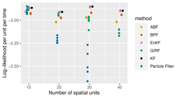
Figure 4: Log-likelihood estimates for 5 replications of ABF, BPF, EnKF, GIRF and particle filter on correlated Brownian motions of various dimensions. The Kalman filter (KF) provides the exact likelihood in this case.

Even for methods designed to be scalable, Monte Carlo variance can be expected to grow with the size of the dataset, and approximations used to enhance scalability may result in bias. Figure 4 investigates how the accuracy of the likelihood estimate scales with $U$ for the bm model. Since class ‘spatPomp’ inherits from class ‘pomp’, we can compare spatPomp methods against the pfilter algorithm from pomp. We see that the performance of pfilter rapidly degrades as dimension increases, whereas the spatPomp methods scale better. On this Gaussian problem, the exact likelihood is available via the Kalman filter, and EnKF is almost exact since the Gaussian approximation used to construct its update rule is correct.

Computing resources used by each algorithm for Figure 4 are given in Table 2. Each algorithm was allowed to use 10 central processing unit (CPU) cores to evaluate all the likelihoods and the algorithmic settings were fixed as shown in the table. CPU time is not necessarily the only relevant consideration, for example, when applying pfilter with a large number of units and a complex model, memory constraints rather than CPU requirements may limit the practical number of particles. By contrast, ABF has a high CPU requirement but it parallelizes easily to take advantage of distributed resources.

The time-complexity of GIRF is quadratic in $U$, due to the intermediate time step loop shown in the pseudocode in Section 3.1, whereas the other algorithms scale linearly with $U$ for a fixed algorithmic setting. However, a positive feature of GIRF is that it shares with PF the property that it targets the exact likelihood, i.e., it is consistent for the exact log likelihood as the number of particles grows and the Monte Carlo variance approaches zero. GIRF may be a practical algorithm when the number of units prohibits PF but permits effective use of GIRF. EnKF and BPF generally run the quickest and require the least memory. However, the Gaussian and independent blocks assumptions, respectively, of the two algorithms must be reasonable to obtain likelihood estimates with low bias. On a new problem, it is advantageous to compare various algorithms to reveal unexpected limitations of the different approximations inherent in each algorithm.

Table 2: Comparison of computational resources of the filtering algorithms

Method	Resources (core-minutes)	Particles (per replicate)	Replicates	Guide particles	Lookahead
Particle Filter	0.89	2000	-	-	-
ABF	47	100	500	-	-
GIRF	12	500	-	50	1
EnKF	1.1	2000	-	-	-
BPF	1.5	2000	-	-	-

5.2 Parameter inference

The correlated Brownian motions example also serves to illustrate parameter inference using IGIRF. Suppose we have data from the correlated 10-dimensional Brownian motions model discussed above. We consider estimation of the parameters $\sigma$, $\tau$ and $\rho$ when that the initial conditions, $\{{X}_{u}(0),u\in 1{\hskip 1.70717pt:\hskip 1.70717pt}U\}$, are known to be zero. We demonstrate a search started at

R> start_params <- c(rho = 0.8, sigma = 0.4, tau = 0.2,
+    X1_0 = 0, X2_0 = 0, X3_0 = 0, X4_0 = 0, X5_0 = 0,
+    X6_0 = 0, X7_0 = 0, X8_0 = 0, X9_0 = 0, X10_0 = 0)

We start with a test of igirf, estimating the parameters $\rho$, $\sigma$ and $\tau$ but not the initial value parameters. We use a computational intensity variable, i, to switch between algorithmic parameter settings. For debugging, testing and code development we use i=1. For a final version of the manuscript, we use i=2.

R> i <- 2
R> ig1 <- igirf(
+    bm10,
+    params=start_params,
+    Ngirf=switch(i,2,50),
+    Np=switch(i,10,1000),
+    Ninter=switch(i,2,5),
+    lookahead=1,
+    Nguide=switch(i,5,50),
+    rw.sd=rw.sd(rho=0.02,sigma=0.02,tau=0.02),
+    cooling.type = "geometric",
+    cooling.fraction.50=0.5
+  )

ig1 is an object of class ‘igirfd_spatpomp’ which inherits from class ‘girfd_spatpomp’. A useful diagnostic of the parameter search is a plot of the change of the parameter estimates during the course of an igirf() run. Each iteration within an igirf run provides a parameter estimate and a likelihood evaluation at that estimate. The plot method for a class ‘igirfd_spatPomp’ object shows the convergence record of parameter estimates and their likelihood evaluations. As shown in Figure 5, this igirf search has allowed us to explore the parameter space and climb significantly up the likelihood surface to within a small neighborhood of the maximum likelihood. The search took 13.0 minutes on one CPU core for this example with 10 spatial units. Investigation of larger models may require multiple searches of the parameter space, started at various points, implemented using parallel runs of igirf().

The log-likelihood plotted in Figure 5, and that computed by logLik(ig1), correspond to the perturbed model. These should be recomputed to obtain a better estimate for the unperturbed model. Different likelihood evaluation methods can be applied, as shown in Section 5.1, to investigate their comparative strengths and weaknesses. For bm10. the model is linear and Gaussian and so the maximum likelihood estimate of our model and the likelihood at this estimate can be found numerically using the Kalman filter. The maximum log likelihood is -373.0, whereas the likelihood obtained by ig1 is -374.2. This shortfall is a reminder that Monte Carlo optimization algorithms should usually be replicated, and should be used with inference methodology that accommodates Monte Carlo error, as discussed in Section 5.3.

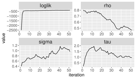
Figure 5: The output of the plot() method on the object of class ‘igirfd_spatPomp’ that encodes our model for correlated Brownian motions produces convergence traces for $\rho$, $\sigma$ and $\tau$, and the corresponding log likelihoods. Over 50 iterations igirf() has allowed us to get within a neighborhood of the maximum likelihood.

5.3 Monte Carlo profiles

Proper interpretation of a parameter estimate requires understanding its uncertainty. Here, we construct a profile likelihood 95% confidence interval for the coupling parameter, $\rho$, in the bm10 model. This entails calculation of the maximized likelihood over all parameters excluding $\rho$, for a range of fixed values of $\rho$. We use Monte Carlo adjusted profile (MCAP) methodology to accommodate Monte Carlo error in maximization and likelihood evaluation (Ionides et al., 2017; Ning et al., 2021).

In practice, we carry out multiple searches for each value of $\rho$, with other parameters drawn at random from a specified hyperbox. We build this box on a transformed scale suitable for optimization, taking advantage of the partrans method. It is generally convenient to optimize non-negative parameters on a log scale and $(0,1)$ valued parameter on a logit scale. We set this up using the pomp function profile_design, taking advantage of the partrans method defined by the partrans argument to spatPomp, defined here as

R> bm10 <- spatPomp(bm10,
+    partrans = parameter_trans(log = c("sigma", "tau"), logit = c("rho")),
+    paramnames = c("sigma","tau","rho")
+  )

This provides access to the partrans method which we use when constructing starting points for the search:

R> theta_lo_trans <- partrans(bm10,coef(bm10),dir="toEst") - log(2)
R> theta_hi_trans <- partrans(bm10,coef(bm10),dir="toEst") + log(2)
R> profile_design(
+    rho=seq(from=0.2,to=0.6,length=10),
+    lower=partrans(bm10,theta_lo_trans,dir="fromEst"),
+    upper=partrans(bm10,theta_hi_trans,dir="fromEst"),
+    nprof=switch(i,2,10)
+  ) -> pd

The argument nprof sets the number of searches, each started at a random starting point, for each value of the profiled parameter, rho. We can apply any of the methods of Section 4 for likelihood maximization and any of the methods of Section 3 for likelihood evaluation. Experimentation is recommended—here, we demonstrate using igirf and enkf. We run parallel searches using foreach and %dopar% from the foreach package (Wallig and Weston, 2020) and collecting all the results together using bind_rows from dplyr (Wickham et al., 2020). Multiple log-likelihood evaluations are carried out on the parameter estimate resulting from each search, averaged using logmeanexp which also provides a standard error.

R> foreach (p=iter(pd,"row"),.combine=dplyr::bind_rows) %dopar% {
+    library(spatPomp)
+    ig2 <- igirf(ig1,params=p,rw.sd=rw.sd(sigma=0.02,tau=0.02))
+    ef <- replicate(switch(i,2,10),enkf(ig2,Np=switch(i,50,2000)))
+    ll <- sapply(ef,logLik)
+    ll <- logmeanexp(ll,se=TRUE)
+    data.frame(as.list(coef(ig2)),loglik=ll[1],loglik.se=ll[2])
+  } -> rho_prof

Above, calling igirf on ig1 imports all the previous algorithmic settings except for those that we explicitly modify. Each row of rho_prof now contains a parameter estimate its log likelihood, with $\rho$ values fixed along a grid. The MCAP 95% confidence interval constructed by mcap uses loess to obtain a smoothed estimate of the profile likelihood function and then determines a confidence interval using by a cutoff based on the delta method applied to a local quadratic regression. This cutoff is typically slightly larger than the asymptotic 1.92 cutoff for a standard profile likelihood confidence interval constructed assuming error-free likelihood maximization and evaluation.

R> rho_mcap <- mcap(rho_prof[,"loglik"],parameter=rho_prof[,"rho"])
R> rho_mcap$ci
[1] 0.2568569 0.5083083

Note that the data in bm10 are generated from a model with $\rho=0.4$.

6 A spatiotemporal model of measles transmission

A spatPomp data analysis may consist of the following major steps: (i) obtain data, postulate a class of models that could have generated the data and bring these two pieces together via a call to spatPomp(); (ii) employ the tools of likelihood-based inference, evaluating the likelihood at specific parameter sets, maximizing likelihoods under the postulated class of models, constructing Monte Carlo adjusted confidence intervals, or performing likelihood ratio hypothesis tests of nested models; (iii) criticize the model by comparing simulations to data, or by considering rival models. In this section, we focus on step (i), showing how to bring data and models together via a metapopulation compartment model for measles dynamics in the 6 largest cities in England in the pre-vaccine era. Tools for step (ii) have been covered in Sections 3 and 4. Step (iii) benefits from the flexibility of the large model class supported by spatPomp.

Compartment models for population dynamics partition the population into categories called compartments. Individuals may move between compartments, and the rate of flow of individuals between a pair of compartments may depend on the number of individuals in other compartments. Compartment models have widespread scientific applications, especially in the biological and health sciences (Bretó et al., 2009). Spatiotemporal compartment models can be called patch models or metapopulation models in an ecological context, where each spatial unit is called a patch or a sub-population. We present a spatiotemporal model for disease transmission dynamics of measles within and between multiple cities, based on the model of Park and Ionides (2020) which adds spatial interaction to the compartment model presented by He et al. (2010). We write equations for a SpatPOMP model contructed by the measles() and he10 functions in spatPomp construct. This illustrates how spatPomp can accommodate various model features that may be relevant for a successful statistical description of epidemiological metapopulation dynamics. We then demonstrate explicitly how to construct a simplified version of this model.

The measles() and he10() models are similar, but differ in details. For measles(), the data consist of biweekly counts and parameters are all shared between units, matching the analysis of Park and Ionides (2020) and Ionides et al. (2021). For he10(), data are weekly and parameters can be shared or unit-specific, matching the analysis of He et al. (2010) and Ionides et al. (2022). We write the model for the general case where all parameters are unit-specific, noting that it is a relevant data analysis question to determine when parameter dependence on $u$ can be omitted.

6.1 Mathematical model for the latent process

We first define the model mathematically, starting with a description of the coupling, corresponding here to travel between cities. Let $v_{u\tilde{u}}$ denote the number of travelers from city $u$ to $\tilde{u}$. Here, $v_{u\tilde{u}}$ follows the gravity model of Xia et al. (2004), with $v_{u\tilde{u}}=g_{u}V_{u\tilde{u}}$ where $g_{u}$ is called a gravitation parameter and

$$V_{u\tilde{u}}=\frac{\mathrm{pop}_{u}\cdot\mathrm{pop}_{\tilde{u}}}{\mathrm{dist}(u,\tilde{u})}\times\frac{\;\overline{\mathrm{dist}}\;}{\;\,\overline{\mathrm{pop}}^{2}\,\;}.$$

Here, $\mathrm{dist}(u,\tilde{u})$ denotes the distance between city $u$ and city $\tilde{u}$, $\mathrm{pop}_{u}$ is the average across time of the census population $P_{u}(t)$ for city $u$, $\overline{\mathrm{pop}}$ is the average of $\mathrm{pop}_{u}$ across cities, and $\overline{\mathrm{dist}}$ is the average of $\mathrm{dist}(u,\tilde{u})$ across pairs of cities.

The measles model divides the population of each city into susceptible, $S$, exposed, $E$, infectious, $I$, and recovered/removed, $R$, compartments. The number of individuals in each compartment for city $u$ at time $t$ are denoted by $S_{u}(t)$, $E_{u}(t)$, $I_{u}(t)$, and $R_{u}(t)$. The latent state is $\boldsymbol{X}(t)=\big{(}X_{1}(t),\dots,X_{U}(t)\big{)}$ with $X_{u}(t)=\big{(}S_{u}(t),E_{u}(t),I_{u}(t),R_{u}(t)\big{)}$. The dynamics of the latent state can be written in terms of flows between compartments, together with flows into and out of the system, as follows:

$$\left.\begin{array}[]{lllllll}\displaystyle dS_{u}(t)&=&dN_{BS,u}(t)&-&dN_{SE,u}(t)&-&dN_{SD,u}(t)\\ \displaystyle dE_{u}(t)&=&dN_{SE,u}(t)&-&dN_{EI,u}(t)&-&dN_{ED,u}(t)\\ \displaystyle dI_{u}(t)&=&dN_{EI,u}(t)&-&dN_{IR,u}(t)&-&dN_{ID,u}(t)\end{array}\qquad\right\}\quad\mbox{for $u=1,\dots,U$.}$$

Here, $N_{SE,u}(t)$, $N_{EI,u}(t)$, and $N_{IR,u}(t)$ are counting process corresponding to the cumulative number of individuals transitioning between the compartments identified by the subscripts. The recruitment of susceptible individuals into city $u$ is denoted by the counting process $N_{BS,u}(t)$, primarily modeling births. Each compartment also has an outflow, written as a transition to $D$, primarily representing death, which occurs at a constant per-capita rate $\mu$. The number of recovered individuals $R_{u}(t)$ in city $u$ is defined implicitly from $P_{u}(t)=S_{u}(t)+E_{u}(t)+I_{u}(t)+R_{u}(t)$. $R_{u}(t)$ plays no direct role in the dynamics, beyond accounting for individuals not in any of the other classes.

To define the Markov model, we specify a rate for each counting process. Thus, $\mu_{EI,u}$ is the rate at which an individual in $E$ progresses to $I$ in city $u$, and $1/\mu_{EI,u}$ is called the mean disease latency. Similarly, $1/\mu_{IR,u}$ is the mean infectious period. The mortality rates are fixed at $\mu_{SD,u}=\mu_{ED,u}=\mu_{ID,u}=\mu_{RD,u}=\mu_{D}$, with life expectancy $1/\mu_{D}=50\,\mathrm{yr}$. The rate of recruitment of susceptible individuals, $\mu_{BS,u}(t)$, is treated as a covariate defined in terms of the birth rate, $b_{u}(t)$, known from public records. Specifically,

$$\mu_{BS,u}(t)=b_{u}(t-t_{b})\big{[}(1-c_{u})+c_{u}\,\delta(t-t_{a})\big{]},$$

where $t_{a}=\lfloor t\rfloor+252/365$ is the school admission date for the year containing $t$, $t_{b}=4\,\mathrm{yr}$ is a fixed delay between birth and entry into the high-transmission community, $c_{u}$ is a fraction of the births which join the $S$ on their first day of school, and $\delta$ is the Dirac delta function. All rates other than $\mu_{BS,u}$ are defined per capita. The disease transmission rate, $\mu_{SE,u}$, is parameterized as

$$\mu_{SE,u}(t)=\overline{\beta}_{u}\,\mathrm{seas}_{u}(t)\left[\left(\frac{I_{u}(t)+\iota_{u}}{P_{u}(t)}\right)^{\alpha_{u}}+\sum_{\tilde{u}\neq u}\frac{v_{u\tilde{u}}}{P_{u}(t)}\left\{\left(\frac{I_{\tilde{u}}(t)}{P_{\tilde{u}}(t)}\right)^{\alpha_{\tilde{u}}}-\left(\frac{I_{u}(t)}{P_{u}(t)}\right)^{\alpha_{u}}\right\}\right]\frac{d\Gamma_{SE,u}}{dt},$$

where the mean transmission rate, $\overline{\beta}_{u}$, is parameterized as $\overline{\beta}_{u}=\mathcal{R}_{0,u}(\mu_{IR,u}+\mu_{D})$ with $\mathcal{R}_{0,u}$ being the basic reproduction rate; $\mathrm{seas}_{u}(t)$ is a periodic step function taking value $(1-A_{u})$ during school vacations and $(1+0.381\,A_{u})$ during school terms, defined so that the average value of $\mathrm{seas}_{u}(t)$ is 1; $\alpha_{u}$ is an exponent describing non-homogeneous mixing of individuals; $\iota_{u}$ describes infected individuals ariving from outside the study population; the multiplicative white noise $d\Gamma_{SE,u}/dt$ is a derivative of a gamma process $\Gamma_{SE,u}(t)$ having independent gamma distributed increments with $\E[\Gamma_{SE,u}(t)]=t$ and $\mathrm{Var}[\Gamma_{SE,u}(t)]=\sigma^{2}_{SE,u}t$, where $\sigma^{2}_{SE,u}$ is the infinitesimal variance of the noise. The formal meaning of $d\Gamma_{SE,u}/dt$ as white noise on the rate of a Markov chain was developed by Bretó et al. (2009) and Bretó and Ionides (2011). In brief, an Euler numerical solution depends on the rate function integrated over a small time interval of length $\Delta t$. The integrated noise process is an increment of the gamma process, and these increments are independent gamma random variables. The continuous time Markov chain corresponding to this noisy rate is the limit of the Euler solutions as $\Delta t\rightarrow 0$, and so these Euler solutions provide a practical approach to working with the model. A single Euler step is defined via the Csnippet for rprocess, below. This code involves use of the reulermultinom function, which is the C interface to the R function reulermultinom provided by pomp. It keeps track of all the rates for possible departures from a compartment. The gamma white noise in these rates is added using the rgammawn function, which is also defined by pomp in both C and R.

Multiplicative white noise provides a way to model over-dispersion, a phenomenon where data variability is larger than can be explained by binomial or Poisson approximations. Over-dispersion on a multiplicative scale is also called environmental stochasticity, or logarithmic noise, or extra-demographic stochasticity. Over-dispersion is well established for generalized linear models (McCullagh and Nelder, 1989) and has become increasingly apparent for compartment models as methods have become available to address it Bjørnstad and Grenfell (2001); He et al. (2010); Stocks et al. (2020).

Initial conditions for the latent state process at a time $t_{0}$ are described in terms of initial value parameters, $S_{u,0}$, $E_{u,0}$ and $I_{u,0}$, defined as follows:

$$\begin{array}[]{rclrcl}S_{u}(t_{0})&=&\mathrm{round}\big{(}S_{u,0}\,P_{u}(t_{0})\big{)},&\hskip 14.22636ptE_{u}(t_{0})&=&\mathrm{round}\big{(}E_{u,0}\,P_{u}(t_{0})\big{)},\\ I_{u}(t_{0})&=&\mathrm{round}\big{(}I_{u,0}\,P_{u}(t_{0})\big{)},&R_{u}(t_{0})&=&P_{u}(t_{0})-S_{u}(t_{0})-E_{u}(t_{0})-I_{u}(t_{0}).\end{array}$$

The observations for city $u$ are bi-weekly reports of new cases. We model the total new cases in an interval by keeping track of transitions from $I$ to $R$, since we expect that identified cases will typically be isolated from susceptible individuals. Therefore, we introduce a new latent variable, defined at observation times as

$$C_{u,n}=N_{IR,u}(t_{n})-N_{IR,u}(t_{n-1}).$$

To work with $C_{u,n}$ in the context of a SpatPOMP model, we note that this variable has Markovian dynamics corresponding to a continuous time variable $C_{u}(t)$ satisfying $dC_{u}(t)=dN_{IR,u}(t)$ with the additional property that we set $C_{u}(t)=0$ immediately after an observation time. To model the observation process, we define $Y_{u,n}$ as a normal approximation to an over-dispersed binomial sample of $C_{u,n}$ with reporting rate $\rho_{u}$. Specifically, conditional on $C_{u,n}=c_{u,n}$,

$$Y_{u,n}\sim{\mathrm{Normal}}\big{[}\rho_{u}\,c_{u,n},\rho\,(1-\rho_{u})\,c_{u,n}+\tau^{2}\rho_{u}^{2}c_{u_{n}}^{2}\big{]},$$

where $\tau$ is a measurement overdispersion parameter.

6.2 Construction of a measles spatPomp object

We construction the model described in Section 6.1 for the simplified situation where $\alpha_{u}=1$, $\iota_{u}=0$ and $c_{u}=0$. All other parameters have shared value across units, except for the initial value parameters. A complete spatPomp representation of the model is provided in the source code for he10().

We use the bi-weekly measles case counts from $U=6$ cities in England as reported by Dalziel et al. (2016), provided in the object measles_cases. Each city has about 15 years (391 bi-weeks) of data, with no missing data. The first three rows of this data are shown below, with the year column corresponding to the observation date in years.

     year       city cases
 1950.000     LONDON    96
 1950.000 BIRMINGHAM   179
 1950.000  LIVERPOOL   533
 1950.000 MANCHESTER    22
 1950.000      LEEDS    17
 1950.000  SHEFFIELD    48
 1950.038     LONDON    60
 1950.038 BIRMINGHAM   160

We can construct a spatPomp object by supplying three minimal requirements in addition to our data above: the column names corresponding to the units labels (‘city’) and observation times (‘year’) and the time at which the latent dynamics are initialized. Here we set this to two weeks before the first recorded observations.

R> measles6 <- spatPomp(
+    data=measles_cases,
+    units=’city’,
+    times=’year’,
+    t0=min(measles_cases$year)-1/26
+  )

Internally, unit names are mapped to an index $1,\dots,U$. The number assigned to each unit can be checked by inspecting their position in unit_names(measles). We proceed to collect together further model components, which we will add to measles6 by a subsequent call to spatPomp(). First, we suppose that we have covariate time series, consisting of census population, $P_{u}(t)$, and lagged birthrate, $b_{u}(t-t_{b})$, in a class ‘data.frame’ object called measles_covar. The required format is similar to the data argument, though the times do not have to correspond to observation times since spatPomp will interpolate the covariates as needed.

 year       city lag_birthrate         P
 1950     LONDON      66318.99 3389306.0
 1950 BIRMINGHAM      22968.58 1117892.5
 1950  LIVERPOOL      18732.87  802064.9

We now move on to specifying our model components as Csnippets. To get started, we define the movement matrix $\big{(}v_{u,\tilde{u}}\big{)}_{u,\tilde{u}\in 1{\hskip 1.70717pt:\hskip 1.70717pt}U}$ as a global variable in C that will be accessible to all model components, via the globals argument to spatPomp().

R> measles_globals <- spatPomp_Csnippet("
+    const double V[6][6] = {
+    {0,2.42,0.950,0.919,0.659,0.786},
+    {2.42,0,0.731,0.722,0.412,0.590},
+    {0.950,0.731,0,1.229,0.415,0.432},
+    {0.919,0.722,1.229,0,0.638,0.708},
+    {0.659,0.412,0.415,0.638,0,0.593},
+    {0.786,0.590,0.432,0.708,0.593,0}
+    };
+  ")

We now construct a Csnippet for initializing the latent process at time $t_{0}$. This is done using unit-specific IVPs, as discussed in Sections 2.4 and 2.5. Here, the IVPs are S1_0$,\dots,$S6_0, E1_0,$\dots$,E6_0, and I1_0,$\dots$,I6_0. These code for the initial value of the corresponding states, S1,$\dots$,S6, E1,$\dots$,E6, and I1,$\dots$,I6. Additional book-keeping states, C1,$\dots$,C6, count accumulated cases during an observation interval and so are initialized to zero. The arguments unit_ivpnames = c(’S’,’E’,’I’) and unit_statenames = c(’S’,’E’,’I’,’C’) enable spatPomp() to expect these variables and define then as needed when compiling the Csnippets. Similarly, unit_covarnames = ’P’ declares the corresponding unit-specific population covariate. This is demonstrated in the following Csnippet specifying rinit.

R> measles_rinit <- spatPomp_Csnippet(
+    unit_statenames = c(’S’,’E’,’I’,’C’),
+    unit_ivpnames = c(’S’,’E’,’I’),
+    unit_covarnames = c(’P’),
+    code = "
+      for (int u=0; u<U; u++) {
+        S[u] = round(P[u]*S_0[u]);
+        E[u] = round(P[u]*E_0[u]);
+        I[u] = round(P[u]*I_0[u]);
+        C[u] = 0;
+      }
+    "
+  )

The rprocess Csnippet has to encode only a rule for a single Euler increment from the process model. C definitions are provided by spatPomp for all parameters, state variables, covariates, t, dt and U. Any additional variables required must be declared as C variables within the Csnippet.

R> measles_rprocess <- spatPomp_Csnippet(
+    unit_statenames = c(’S’,’E’,’I’,’C’),
+    unit_covarnames = c(’P’,’lag_birthrate’),
+    code = "
+      double beta, seas, Ifrac, mu[7], dN[7];
+      int u, v;
+      int BS=0, SE=1, SD=2, EI=3, ED=4, IR=5, ID=6;
+
+      beta = R0*(muIR+muD);
+      t = (t-floor(t))*365.25;
+      seas = (t>=7&&t<=100)||(t>=115&&t<=199)||(t>=252&&t<=300)||(t>=308&&t<=356)
+        ? 1.0 + A * 0.2411/0.7589 : 1.0 - A;
+
+      for (u = 0 ; u < U ; u++) {
+        Ifrac = I[u]/P[u];
+        for (v=0; v < U ; v++) if(v != u)
+          Ifrac += g * V[u][v]/P[u] * (I[v]/P[v] - I[u]/P[u]);
+
+        mu[BS] = lag_birthrate[u];
+        mu[SE] = beta*seas*Ifrac*rgammawn(sigmaSE,dt)/dt;
+        mu[SD] = muD;
+        mu[EI] = muEI;
+        mu[ED] = muD;
+        mu[IR] = muIR;
+        mu[ID] = muD;
+
+        dN[BS] = rpois(mu[BS]*dt);
+        reulermultinom(2,S[u],&mu[SE],dt,&dN[SE]);
+        reulermultinom(2,E[u],&mu[EI],dt,&dN[EI]);
+        reulermultinom(2,I[u],&mu[IR],dt,&dN[IR]);
+
+        S[u] += dN[BS] - dN[SE] - dN[SD];
+        E[u] += dN[SE] - dN[EI] - dN[ED];
+        I[u] += dN[EI] - dN[IR] - dN[ED];
+        C[u] += dN[EI];
+      }
+    "
+  )

The measurement model is chosen to allow for overdispersion relative to the binomial distribution with success probability $\rho$. Here, we show the Csnippet defining the unit measurement model. The lik variable is pre-defined and is set to the evaluation of the unit measurement density in either the log or natural scale depending on the value of give_log.

R> measles_dunit_measure <- spatPomp_Csnippet("
+    double m = rho*C;
+    double v = m*(1.0-rho+psi*psi*m);
+    lik = dnorm(cases,m,sqrt(v),give_log);
+  ")

The user may also directly supply dmeasure that returns the product of unit-specific measurement densities. The latter is needed to apply pomp functions which require dmeasure rather than dunit_measure. We create the corresponding Csnippet in measles_dmeasure, but do not display the code here. Next, we construct a Csnippet to code runit_measure,

R> measles_runit_measure <- spatPomp_Csnippet("
+    double cases;
+    double m = rho*C;
+    double v = m*(1.0-rho+psi*psi*m);
+    cases = rnorm(m,sqrt(v));
+    if (cases > 0.0) cases = nearbyint(cases);
+    else cases = 0.0;
+  ")

We also construct, but do not display, a Csnippet measles_rmeasure coding the class ‘pomp’ version rmeasure. Next, we build Csnippets for eunit_measure and vunit_measure which are required by EnKF and IEnKF. These have defined variables named ey and vc respectively, which should return $\E[Y_{u,n}{\,|\,}X_{u,n}]$ and $\mathrm{Var}[Y_{u,n}{\,|\,}X_{u,n}]$. For our measles model, we have

R> measles_eunit_measure <- spatPomp_Csnippet("ey = rho*C;")
R> measles_vunit_measure <- spatPomp_Csnippet("
+    double m = rho*C;
+    vc = m*(1.0-rho+psi*psi*m);
+  ")

It is convenient (but not necessary) to supply a parameter vector of scientific interest for testing the model. Here, we use a parameter vector with duration of infection and latent period both set equal to one week, following Xia et al. (2004), and the basic reproduction number set to $\mathcal{R}_{0}=30$. The gravitational constant, $g=1500$, was picked by qualitative visual matching of simulations.

R> IVPs <- rep(c(0.032,0.00005,0.00004,0.96791),each=6)
R> names(IVPs) <- paste0(rep(c(’S’,’E’,’I’,’R’),each=6),1:6,"_0")
R> measles_params <- c(R0=30,A=0.5,muEI=52,muIR=52,muD=0.02,
+    alpha=1,sigmaSE=0.01,rho=0.5,psi=0.1,g=1500,IVPs)

Special treatment is afforded to latent states that track accumulations of other latent states between observation times. These accumulator variables should be reset to zero at each observation time. The unit_accumvars argument provides a facility to specify the unit-level names of accumulator variables, extending the accumvars argument to pomp(). Here, there is one accumulator variable, C, which is needed since each case report corresponds to new reported infections accumulated over a measurement interval. The pieces of the SpatPOMP are now added to measles6 via a call to spatPomp:

R> measles6 <- spatPomp(
+    data = measles6,
+    covar = measles_covar,
+    unit_statenames = c(’S’,’E’,’I’,’R’,’C’),
+    unit_accumvars = c(’C’),
+    paramnames = names(measles_params),
+    rinit = measles_rinit,
+    rprocess = euler(measles_rprocess, delta.t=1/365),
+    dunit_measure = measles_dunit_measure,
+    eunit_measure = measles_eunit_measure,
+    vunit_measure = measles_vunit_measure,
+    runit_measure = measles_runit_measure,
+    dmeasure = measles_dmeasure,
+    rmeasure = measles_rmeasure,
+    globals = measles_globals
+  )

Here, we have not filled the skeleton and munit_measure arguments, used by girf and abfir. These can be found in the spatPomp package source code for measles().

In Figure 6, we compare a simulation from measles6 with the data. Epidemiological settings may be clearer when looking on the log scale, and so we use the log=TRUE argument to plot(). This figure shows some qualitative similarity between the simulations and the data, with opportunity for future work to investigate discrepancies.

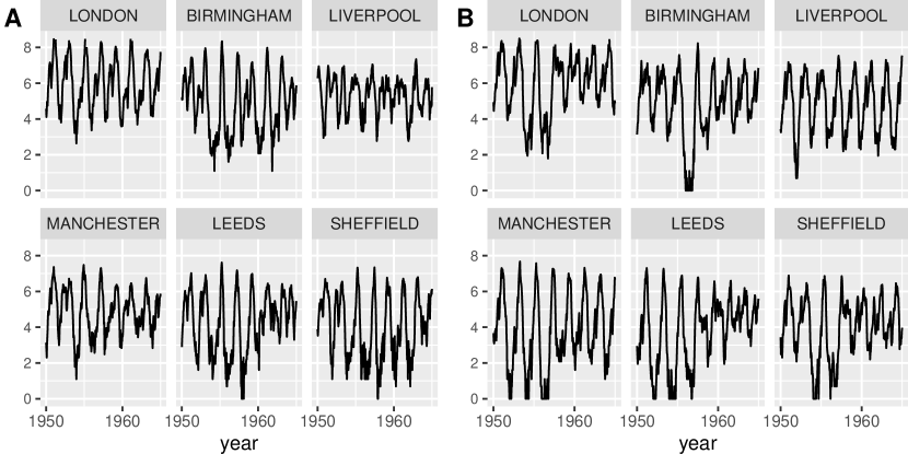
Figure 6: A: reported measles cases in two week intervals for the six largest cities in England, plot(measles6,log=TRUE). B: simulated data, plot(simulate(measles6),log=TRUE). The vertical scale is log(cases+1).

7 Conclusion

The spatPomp package is both a tool for data analysis based on SpatPOMP models and a principled computational framework for the ongoing development of inference algorithms. To date, spatPomp has focused on algorithms with the plug-and-play property, but the package is designed to support new algorithms with and without this property. Current examples have emphasized biological metapopulation dynamics, but diverse applications fit into the SpatPOMP model class. Spatiotemporal data analysis using mechanistic models is a nascent topic, and future methodological developments are anticipated. Since the mission of spatPomp is to be a home for such analyses, the package developers welcome contributions and collaborations to further expand the functionality of spatPomp.

Complex models and large datasets can challenge available computational resources. With this in mind, key components of the spatPomp package and associated models are written in C. This permits competitive performance on benchmarks (FitzJohn et al., 2020) within an R environment. The use of multi-core computing is helpful for computationally intensive methods. Two common computationally intensive tasks in spatPomp are the assessment of Monte Carlo variability and the investigation of the roles of starting values and other algorithmic settings on optimization routines. These tasks require only embarrassingly parallel computations and need no special discussion here.

Practical modeling and inference for metapopulation systems, capable of handling scientifically motivated nonlinear, non-stationary stochastic models, is the last open problem of the challenges raised by Bjørnstad and Grenfell (2001). Recent studies have reiterated the need for such methods, and made some progress toward attaining them (Becker et al., 2016; Li et al., 2020). The spatPomp package provides a unifying framework, facilitating ongoing model development and methodological advances for SpatPOMP models. Everyone whose research involves SpatPOMP models is welcome to contribute new models and statistical methods to spatPomp.

References

- Anderson et al. (2009) Anderson J, Hoar T, Raeder K, Liu H, Collins N, Torn R, Avellano A (2009). “The data assimilation research testbed: A community facility.” Bulletin of the American Meteorological Society, 90(9), 1283–1296. 10.1175/2009BAMS2618.1.
- Arulampalam et al. (2002) Arulampalam MS, Maskell S, Gordon N, Clapp T (2002). “A tutorial on particle filters for online nonlinear, non-Gaussian Bayesian tracking.” IEEE Transactions on Signal Processing, 50, 174–188. 10.1109/78.978374.
- Bakker et al. (2016) Bakker KM, Martinez-Bakker ME, Helm B, Stevenson TJ (2016). “Digital epidemiology reveals global childhood disease seasonality and the effects of immunization.” Proceedings of the National Academy of Sciences of the USA, 113(24), 6689–6694. 10.1073/pnas.1523941113.
- Becker et al. (2016) Becker AD, Birger RB, Teillant A, Gastanaduy PA, Wallace GS, Grenfell BT (2016). “Estimating enhanced prevaccination measles transmission hotspots in the context of cross-scale dynamics.” Proceedings of the National Academy of Sciences, 113(51), 14595–14600. 10.1073/pnas.1604976113.
- Becker et al. (2019) Becker AD, Wesolowski A, Bjørnstad ON, Grenfell BT (2019). “Long-term dynamics of measles in London: Titrating the impact of wars, the 1918 pandemic, and vaccination.” PLoS Computational Biology, 15(9), e1007305. 10.1371/journal.pcbi.1007305.
- Bengtsson et al. (2008) Bengtsson T, Bickel P, Li B (2008). “Curse-of-dimensionality revisited: Collapse of the particle filter in very large scale systems.” In T Speed, D Nolan (eds.), Probability and Statistics: Essays in Honor of David A. Freedman, pp. 316–334. Institute of Mathematical Statistics, Beachwood, OH. 10.1214/193940307000000518.
- Bhadra et al. (2011) Bhadra A, Ionides EL, Laneri K, Pascual M, Bouma M, Dhiman RC (2011). “Malaria in northwest India: Data analysis via partially observed stochastic differential equation models driven by Lévy noise.” Journal of the American Statistical Association, 106, 440–451. 10.1198/jasa.2011.ap10323.
- Bjørnstad and Grenfell (2001) Bjørnstad ON, Grenfell BT (2001). “Noisy clockwork: Time series analysis of population fluctuations in animals.” Science, 293, 638–643. 10.1126/science.1062226.
- Blackwood et al. (2013a) Blackwood JC, Cummings DAT, Broutin H, Iamsirithaworn S, Rohani P (2013a). “Deciphering the impacts of vaccination and immunity on pertussis epidemiology in Thailand.” Proceedings of the National Academy of Sciences of the USA, 110, 9595–9600. 10.1073/pnas.1220908110.
- Blackwood et al. (2013b) Blackwood JC, Streicker DG, Altizer S, Rohani P (2013b). “Resolving the roles of immunity, pathogenesis, and immigration for rabies persistence in vampire bats.” Proceedings of the National Academy of Sciences of the USA. 10.1073/pnas.1308817110.
- Blake et al. (2014) Blake IM, Martin R, Goel A, Khetsuriani N, Everts J, Wolff C, Wassilak S, Aylward RB, Grassly NC (2014). “The role of older children and adults in wild poliovirus transmission.” Proceedings of the National Academy of Sciences of the USA, 111(29), 10604–10609. 10.1073/pnas.1323688111.
- Bretó (2014) Bretó C (2014). “On idiosyncratic stochasticity of financial leverage effects.” Statistics & Probability Letters, 91, 20–26. 10.1016/j.spl.2014.04.003.
- Bretó et al. (2009) Bretó C, He D, Ionides EL, King AA (2009). “Time series analysis via mechanistic models.” Annals of Applied Statistics, 3, 319–348. 10.1214/08-AOAS201.
- Bretó and Ionides (2011) Bretó C, Ionides EL (2011). “Compound Markov counting processes and their applications to modeling infinitesimally over-dispersed systems.” Stochastic Processes and their Applications, 121, 2571–2591. 10.1016/j.spa.2011.07.005.
- Brown et al. (2018) Brown GD, Porter AT, Oleson JJ, Hinman JA (2018). “Approximate Bayesian computation for spatial SEIR(S) epidemic models.” Spatial and Spatio-temporal Epidemiology, 24, 27–37. 10.1016/j.sste.2017.11.001.
- Buhnerkempe et al. (2017) Buhnerkempe MG, Prager KC, Strelioff CC, Greig DJ, Laake JL, Melin SR, DeLong RL, Gulland F, Lloyd-Smith JO (2017). “Detecting signals of chronic shedding to explain pathogen persistence: Leptospira interrogans in California sea lions.” Journal of Animal Ecology, 86(3), 460–472. 10.1111/1365-2656.12656.
- Cappello et al. (2020) Cappello C, De Iaco S, Posa D (2020). “covatest: An R Package for Selecting a Class of Space-Time Covariance Functions.” Journal of Statistical Software, 94(1), 1–42. 10.18637/jss.v094.i01.
- Chambers (1998) Chambers JM (1998). Programming with Data: A Guide to the S Language. Springer Science & Business Media.
- Dalziel et al. (2016) Dalziel BD, Bjørnstad ON, van Panhuis WG, Burke DS, Metcalf CJE, Grenfell BT (2016). “Persistent chaos of measles epidemics in the prevaccination United States caused by a small change in seasonal transmission patterns.” PLoS Computational Biology, 12(2), e1004655. 10.1371/journal.pcbi.1004655.
- Del Moral and Murray (2015) Del Moral P, Murray LM (2015). “Sequential Monte Carlo with highly informative observations.” Journal on Uncertainty Quantification, 3, 969–997. 10.1137/15M1011214.
- Doucet and Johansen (2011) Doucet A, Johansen A (2011). “A tutorial on particle filtering and smoothing: Fifteen years later.” In D Crisan, B Rozovsky (eds.), Oxford Handbook of Nonlinear Filtering. Oxford University Press.
- Earn et al. (2012) Earn DJ, He D, Loeb MB, Fonseca K, Lee BE, Dushoff J (2012). “Effects of school closure on incidence of pandemic influenza in Alberta, Canada.” Annals of Internal Medicine, 156, 173–181. 10.7326/0003-4819-156-3-201202070-00005.
- Evensen (1994) Evensen G (1994). “Sequential data assimilation with a nonlinear quasi-geostrophic model using Monte Carlo methods to forecast error statistics.” Journal of Geophysical Research: Oceans, 99(C5), 10143–10162. 10.1029/94JC00572.
- Evensen and van Leeuwen (1996) Evensen G, van Leeuwen PJ (1996). “Assimilation of geostat altimeter data for the Agulhas Current using the ensemble Kalman filter with a quasigeostrophic model.” Monthly Weather Review, 124, 58–96. 10.1175/1520-0493(1996)124<0085:AOGADF>2.0.CO;2.
- Fasiolo et al. (2016) Fasiolo M, Pya N, Wood SN (2016). “A comparison of inferential methods for highly nonlinear state space models in ecology and epidemiology.” Statistical Science, 31(1), 96–118. 10.1214/15-STS534.
- FitzJohn et al. (2020) FitzJohn RG, Knock ES, Whittles LK, Perez-Guzman PN, Bhatia S, Guntoro F, Watson OJ, Whittaker C, Ferguson NM, Cori A, Baguelin M, Lees JA (2020). “Reproducible parallel inference and simulation of stochastic state space models using odin, dust, and mcstate.” Wellcome Open Research, 5. 10.12688/wellcomeopenres.16466.2.
- Genolini (2008) Genolini C (2008). “A (not so) short introduction to S4.” Technical report, The R-Project for Statistical Computing. URL http://christophe.genolini.free.fr/webTutorial/S4tutorialV0-5en.pdf.
- He et al. (2013) He D, Dushoff J, Day T, Ma J, Earn DJD (2013). “Inferring the causes of the three waves of the 1918 influenza pandemic in England and Wales.” Proceedings of the Royal Society of London, Series B, 280, 20131345. 10.1098/rspb.2013.1345.
- He et al. (2010) He D, Ionides EL, King AA (2010). “Plug-and-play inference for disease dynamics: Measles in large and small towns as a case study.” Journal of the Royal Society Interface, 7, 271–283. 10.1098/rsif.2009.0151.
- Ionides et al. (2021) Ionides EL, Asfaw K, Park J, King AA (2021). “Bagged filters for partially observed interacting systems.” Journal of the American Statistical Association, pre-published online. 10.1080/01621459.2021.1974867.
- Ionides et al. (2017) Ionides EL, Breto C, Park J, Smith RA, King AA (2017). “Monte Carlo profile confidence intervals for dynamic systems.” Journal of the Royal Society Interface, 14, 1–10. 10.1098/rsif.2017.0126.
- Ionides et al. (2015) Ionides EL, Nguyen D, Atchadé Y, Stoev S, King AA (2015). “Inference for dynamic and latent variable models via iterated, perturbed Bayes maps.” Proceedings of the National Academy of Sciences of the USA, 112(3), 719––724. 10.1073/pnas.1410597112.
- Ionides et al. (2022) Ionides EL, Ning N, Wheeler J (2022). “An Iterated Block Particle Filter for Inference on Coupled Dynamic Systems with Shared and Unit-Specific Parameters.” Statistica Sinica, pre-published online. 10.5705/ss.202022.0188.
- Johansen and Doucet (2008) Johansen AM, Doucet A (2008). “A note on the auxiliary particle filter.” Statistics & Probability Letters, 78, 1498–1504. 10.1016/j.spl.2008.01.032.
- Kain et al. (2021) Kain MP, Childs ML, Becker AD, Mordecai EA (2021). “Chopping the tail: How preventing superspreading can help to maintain COVID-19 control.” Epidemics, 31, 100430. 10.1016/j.epidem.2020.100430.
- Kantas et al. (2015) Kantas N, Doucet A, Singh SS, Maciejowski J, Chopin N, et al. (2015). “On particle methods for parameter estimation in state-space models.” Statistical Science, 30(3), 328–351. 10.1214/14-STS511.
- Katzfuss et al. (2020) Katzfuss M, Stroud JR, Wikle CK (2020). “Ensemble Kalman methods for high-dimensional hierarchical dynamic space-time models.” Journal of the American Statistical Association, 115(530), 866–885. 10.1080/01621459.2019.1592753.
- King et al. (2008) King AA, Ionides EL, Pascual M, Bouma MJ (2008). “Inapparent infections and cholera dynamics.” Nature, 454, 877–880. 10.1038/nature07084.
- King et al. (2016) King AA, Nguyen D, Ionides EL (2016). “Statistical inference for partially observed Markov processes via the R Package pomp.” Journal of Statistical Software, 69, 1–43. 10.18637/jss.v069.i12.
- Li et al. (2020) Li R, Pei S, Chen B, Song Y, Zhang T, Yang W, Shaman J (2020). “Substantial undocumented infection facilitates the rapid dissemination of novel coronavirus (SARS-CoV-2).” Science, 368(6490), 489–493. 10.1126/science.abb3221.
- Lorenz (1996) Lorenz EN (1996). “Predictability: A problem partly solved.” Proceedings of the Seminar on Predictability, 1, 1–18.
- Marino et al. (2019) Marino JA, Peacor SD, Bunnell D, Vanderploeg HA, Pothoven SA, Elgin AK, Bence JR, Jiao J, Ionides EL (2019). “Evaluating consumptive and nonconsumptive predator effects on prey density using field time-series data.” Ecology, 100(3), e02583. 10.1002/ecy.2583.
- Martinez-Bakker et al. (2015) Martinez-Bakker M, King AA, Rohani P (2015). “Unraveling the transmission ecology of polio.” PLoS Biology, 13(6), e1002172. 10.1371/journal.pbio.1002172.
- McCullagh and Nelder (1989) McCullagh P, Nelder JA (1989). Generalized Linear Models. 2nd edition. Chapman and Hall, London.
- Michaud et al. (2021) Michaud N, de Valpine P, Turek D, Paciorek CJ, Nguyen D (2021). “Sequential Monte Carlo methods in the nimble and nimbleSMC R Packages.” Journal of Statistical Software, 100, 1–39. 10.18637/jss.v100.i03.
- Murray (2015) Murray LM (2015). “Bayesian state-space modelling on high-performance hardware using LibBi.” Journal of Statistical Software, 67(10), 1–36. 10.18637/jss.v067.i10.
- Ng et al. (2002) Ng B, Peshkin L, Pfeffer A (2002). “Factored particles for scalable monitoring.” Proceedings of the 18th Conference on Uncertainty and Artificial Intelligence, pp. 370–377. 10.5555/2073876.2073920.
- Ning and Ionides (2022a) Ning N, Ionides EL (2022a). “Iterated block particle filter for high-dimensional parameter learning: Beating the curse of dimensionality.” arXiv:2110.10745. 10.48550/arXiv.2110.10745.
- Ning and Ionides (2022b) Ning N, Ionides EL (2022b). “Using an iterated block particle filter via spatPomp.” URL https://kidusasfaw.github.io/spatPomp/.
- Ning et al. (2021) Ning N, Ionides EL, Ritov Y (2021). “Scalable Monte Carlo inference and rescaled local asymptotic normality.” Bernoulli, 27, 2532–2555. 10.3150/20-BEJ1321.
- Park and Ionides (2020) Park J, Ionides EL (2020). “Inference on high-dimensional implicit dynamic models using a guided intermediate resampling filter.” Statistics & Computing, 30, 1497–1522. 10.1007/s11222-020-09957-3.
- Pitt and Shepard (1999) Pitt MK, Shepard N (1999). “Filtering via simulation: Auxillary particle filters.” Journal of the American Statistical Association, 94, 590–599. 10.1080/01621459.1999.10474153.
- Pons-Salort and Grassly (2018) Pons-Salort M, Grassly NC (2018). “Serotype-specific immunity explains the incidence of diseases caused by human enteroviruses.” Science, 361(6404), 800–803. 10.1126/science.aat6777.
- R Core Team (2022) R Core Team (2022). “Writing R extensions.” R Foundation for Statistical Computing. URL https://cran.r-project.org/doc/manuals/R-exts.html.
- Ranjeva et al. (2017) Ranjeva SL, Baskerville EB, Dukic V, Villa LL, Lazcano-Ponce E, Giuliano AR, Dwyer G, Cobey S (2017). “Recurring infection with ecologically distinct HPV types can explain high prevalence and diversity.” Proceedings of the National Academy of Sciences, p. 201714712. 10.1073/pnas.1714712114.
- Rebeschini and van Handel (2015) Rebeschini P, van Handel R (2015). “Can local particle filters beat the curse of dimensionality?” The Annals of Applied Probability, 25(5), 2809–2866. 10.1214/14-AAP1061.
- Roy et al. (2013) Roy M, Bouma MJ, Ionides EL, Dhiman RC, Pascual M (2013). “The potential elimination of Plasmodium vivax malaria by relapse treatment: Insights from a transmission model and surveillance data from NW India.” PLoS Neglected Tropical Diseases, 7, e1979. 10.1371/journal.pntd.0001979.
- Shrestha et al. (2013) Shrestha S, Foxman B, Weinberger DM, Steiner C, Viboud C, Rohani P (2013). “Identifying the interaction between influenza and pneumococcal pneumonia using incidence data.” Science Translational Medicine, 5, 191ra84. 10.1126/scitranslmed.3005982.
- Shrestha et al. (2011) Shrestha S, King AA, Rohani P (2011). “Statistical inference for multi-pathogen systems.” PLoS Computational Biology, 7, e1002135. 10.1371/journal.pcbi.1002135.
- Sigrist et al. (2015) Sigrist F, Kunsch HR, Stahel WA (2015). “spate: An R package for spatio-temporal modeling with a stochastic advection-diffusion process.” Journal of Statistical Software, 63(14), 1–23. 10.18637/jss.v063.i14.
- Snyder et al. (2015) Snyder C, Bengtsson T, Morzfeld M (2015). “Performance bounds for particle filters using the optimal proposal.” Monthly Weather Review, 143(11), 4750–4761. 10.1175/MWR-D-15-0144.1.
- Stocks et al. (2020) Stocks T, Britton T, Höhle M (2020). “Model selection and parameter estimation for dynamic epidemic models via iterated filtering: application to rotavirus in Germany.” Biostatistics, 21(3), 400–416. 10.1093/biostatistics/kxy057.
- Tong (1990) Tong H (1990). Non-linear Time Series: A Dynamical System Approach. Oxford Science Publ., Oxford.
- Wallig and Weston (2019) Wallig M, Weston S (2019). doParallel: Foreach parallel adaptor for the ’parallel’ package. R package version 1.0.15, URL https://CRAN.R-project.org/package=doParallel.
- Wallig and Weston (2020) Wallig M, Weston S (2020). foreach: Provides foreach looping construct. R package version 1.5.0, URL https://CRAN.R-project.org/package=foreach.
- Wickham (2019) Wickham H (2019). Advanced R. CRC press. URL https://adv-r.hadley.nz/.
- Wickham et al. (2020) Wickham H, François R, Henry L, Müller K (2020). dplyr: A Grammar of Data Manipulation. R package version 1.0.0, URL https://CRAN.R-project.org/package=dplyr.
- Wikle et al. (2019) Wikle CK, Zammit-Mangion A, Cressie N (2019). Spatio-temporal Statistics with R. CRC Press.
- Xia et al. (2004) Xia Y, Bjørnstad ON, Grenfell BT (2004). “Measles metapopulation dynamics: A gravity model for epidemiological coupling and dynamics.” American Naturalist, 164(2), 267–281. 10.1086/422341.