A Hybrid Learner for Simultaneous Localization and Mapping

Abstract

Simultaneous localization and mapping (SLAM) is used to predict the dynamic motion path of a moving platform based on the location coordinates and the precise mapping of the physical environment. SLAM has great potential in augmented reality (AR), autonomous vehicles, viz. self-driving cars, drones, Autonomous navigation robots (ANR). This work introduces a hybrid learning model that explores beyond feature fusion and conducts a multimodal weight sewing strategy towards improving the performance of a baseline SLAM algorithm. It carries out weight enhancement of the front end feature extractor of the SLAM via mutation of different deep networks’ top layers. At the same time, the trajectory predictions from independently trained models are amalgamated to refine the location detail. Thus, the integration of the aforesaid early and late fusion techniques under a hybrid learning framework minimizes the translation and rotation errors of the SLAM model. This study exploits some well-known deep learning (DL) architectures, including ResNet18, ResNet34, ResNet50, ResNet101, VGG16, VGG19, and AlexNet for experimental analysis. An extensive experimental analysis proves that hybrid learner (HL) achieves significantly better results than the unimodal approaches and multimodal approaches with early or late fusion strategies. Hence, it is found that the Apolloscape dataset taken in this work has never been used in the literature under SLAM with fusion techniques, which makes this work unique and insightful.

I Introduction

SLAM is a technological process that enables a device to build a map of the environment, at the same time, helps compute the relative location on predefined map. It can be used for range of applications from self-driving vehicles (SDV) to space and maritime exploration, and from indoor positioning to search and rescue operations. The primary responsibility of a SLAM algorithm is to produce an understanding of a moving platform’s environment and the location of the vehicle by providing the value of its coordinates; thus, improving the formation of a trajectory to determine the view at a particular instance. As a SLAM is one of the emerging technologies, numerous implementations have been introduced but the DL-based approaches surmount others by their efficiency in extracting the finest features and giving better results even in a feature-scarce environment.

This study aims to improve the performance of a self-localization module based on PoseNet [1] architecture through the concept of hybrid learning that does a multimodal weight mutation for enhancing the weights of a feature extractor layer and refines the trajectory predictions using amalgamation of multimodal scores. The ablation study is carried out on the Apolloscape [2, 3], as per our knowledge, there has been no research work performed on the self-localization repository of the Apolloscape dataset, in which the proposed HL has been evaluated extensively. The experimental analysis presented in this work consists of three parts, in which initial two parts form the base for the third. The first part concentrates on an extensive evaluation of several DL models, as feature extractors. The second part analyzes of two proposed multimodal fusion approaches: (i). an early fusion via layer weight enhancement of feature extractor, and (ii). a late fusion via score refinement of the trajectory (pose) regressor. Finally, the third part aims at the combination of early and late fusion models forming a hybrid learner with addition or multiplication operation. Here, the late fusion model harnesses five pretrained deep convolutional neural networks (DCNNs), viz. ResNet18, ResNet34, ResNet101. VGG16, and VGG19 as the feature extractor for pose regressor module. While, the early fusion model and the HL focuses on exploiting the best DCNNs, ResNet101 and VGG19 based on their individual performance on the Apolloscape self-localization dataset.

When analyzing the results of the early and late fusion models, it is observed that the early fusion encompasses $14.842m$ of translation error and $0.673^{\circ}$ of rotation error. On the other hand, the late fusion achieves $9.763m$ of translation error and $0.945^{\circ}$ of rotation error. On analyzing the hybrid learners, the additive hybrid learner (AHL) gets $10.400m$ of translation error and $0.828^{\circ}$ of rotation error, whereas the multiplicative hybrid learner (MHL) records $9.307m$ and $1.206^{\circ}$ of translation and rotation errors, respectively. By fusing the predictions of AHL and MHL called hybrid learner full-fusion (HLFF) produces better results than all other models with $7.762m$ and $0.886^{\circ}$ of translation rotation errors, respectively.

The rest of the paper is organized as follows. Section II reviews relevant SLAM literature and provides basic detail of the PoseNet, unimodality, and multimodality. Section III elaborates the proposed hybrid learner including required pre-processing operations. Section IV describes the experimental setup and analyzes the obtained results from various models. Section V concludes the research work.

II Background

II-A SLAM

Simultaneous localization and mapping is an active research domain in robotics and artificial intelligence (AI). It enables a remotely automated moving vehicle to be placed in an unknown environment and location. According to Whyte et al. [4] and Montemerlo et al. [5], SLAM should build a consistent map of this unknown environment and determine the location relative to the map. Through SLAM, robots and vehicles can be truly and completely automated without any or minimal human intervention. But the estimation of maps consists of various other entities, such as large storage issues, precise location coordinates, which makes SLAM a rather intriguing task, especially in the real-time domain.

Many researches have been done worldwide to determine the efficient method to perform SLAM. In [6], Montemerlo et al. propose a model named FastSLAM, as an efficient solution to the problem. FastSLAM is a recursive algorithm that calculates the posterior distribution spanning over autonomous vehicle’s pose and landmark locations, yet, it scales logarithmically with the total number of landmarks. This algorithm relies on an exact factorization of the posterior into a product of landmark distributions and a distribution over the paths of the robot. The research on SLAM originates on the work of Smith and Cheeseman [7] that propose the use of the extended Kalman filter (EKF). It is based on the notion that pose errors and errors in the map are correlated, and the covariance matrix obtained by the EKF represents this covariance. There are two main approaches for the localization of an autonomous vehicle: metric SLAM and appearance-based SLAM [1]. However, this research focuses on the appearance-based SLAM that is trained by giving a set of visual samples collected at multiple discrete locations.

II-B PoseNet

The neural network (NN) comprises of several interconnected nodes and associated parameters, like weights and biases. The weights are adjusted through a series of trials and experiments in the training phase so that the network can learn and can be used to predict the outcomes at a later stage. There are various kinds of NN’s available, for instance, Feed-forward neural network (FFNN), Radial basis neural network (RBNN), DCNN, Recurrent neural network (RNN), etc. Among them, the DCNN’s have been highly regarded for the adaptability and finer interpretability with accurate and justifiable predictions in applications range from finance to medical analysis and from science to engineering. Thus, the PoseNet model for SLAM shown in Fig. 1, harness the DCNN to be firm against difficult lighting, blurredness, and varying camera instincts [1]. Figure 1 depicts the underlying architecture of the PoseNet. It subsumes a front-end with a feature extractor and a back-end with a regression subnetwork. The feature extractor can be a pretrained DCNN, like ResNet$34$, VGG$16$, or AlexNet. The regression subnetwork consists of three stages: a dropout, an average pooling, a dense layer interconnected, sequentially. It receives the high dimensional vector from the feature extractor. Through the average pooling and dropout layers, it is then reduced to a lower dimension for generalization and faster computation [8]. The predicted poses are in Six-degree of freedom (6-DoF), which define the six parameters in translation and rotation [1]. The translation consists of forward-backward, left-right, and up-down parameters forming the axis of 3D space as $x-axis$, $y-axis$, and $z-axis$, respectively. Likewise, the rotation includes yaw, pitch, and roll parameters of the same 3D space noted as $normal-axis$, $transverse-axis$, and $longitudinal-axis$, respectively.

Front-end	Back-end
Feature Extractor:	Pose Regressor	Output: Poses
A pretrained CNN	Dropout$\rightarrow$ Pooling$\rightarrow$ Dense	Translation & Rotation

Figure 1: PoseNet Architecture Subsuming a Feature Extractor and a Pose Regressor Subnetwork.

Then, these six core parameters are converted to seven coordinates: $x_{1}$, $x_{2}$, and $x_{3}$ of translation coordinates, and $y_{1},y_{2},y_{3},y_{4}$ of rotation coordinates. It is because the actual rotation poses are in Euler angles. Thus, a pre-processing operation converts the Euler angles into quaternions. The quaternions are the set of four values ($x_{o}$, $y_{1}$, $y_{2}$ and $y_{3}$), where $x_{o}$ represents a scalar rotation of the vector - $y_{1}$, $y_{2}$ and $y_{3}$. This conversion is governed by the expressions given in Eq. (1) - (4).

$$x_{0}=(\sqrt{1+c_{1}c_{2}+c_{1}c_{3}-s_{1}s_{2}s_{3}+c_{2}c_{3}})/2,$$ (1)

$$y_{1}=(c_{2}s_{3}+c_{1}s_{3}+s_{1}s_{2}c_{3})/4x_{0},$$ (2)

$$y_{2}=(s_{1}c_{2}+s_{1}c_{3}+c_{1}s_{2}s_{3})/4x_{0},$$ (3)

$$y_{3}=(-s_{1}s_{3}+c_{1}s_{2}c_{3}+s_{2})/4x_{0},$$ (4)

where $c_{1}$ = $\cos(roll/2)$, $c_{2}$ = $\cos(yaw/2)$, $c_{3}$ = $\cos(pitch/2)$, $s_{1}$ = $\sin(roll/2)$, $s_{2}$ = $\sin(yaw/2)$, and $s_{3}$ = $\sin(pitch/2)$.

The pose regressor subnetwork is to be trained to minimize the translation and rotation errors. These errors are combined into a single objective function, $L_{\beta}$ as defined in Eq. (5) [9].

$$L_{\beta}(I)=L_{x}(I)+\beta L_{q}(I),$$ (5)

where $L_{x}$, $L_{q}$ are the losses of translation and rotation respectively, and $I$ is the input vector representing the discrete location in the map. $\beta$ is a scaling factor that is used to balance both the losses and calculated using homoscedastic uncertainty that combines the losses as defined in (6).

$$L_{\sigma}(I)=\frac{L_{x}(I)}{\hat{\sigma}_{x}^{2}}+\log\hat{\sigma}_{x}^{2}+\frac{L_{q}(I)}{\hat{\sigma}_{q}^{2}}+\log\hat{\sigma}_{q}^{2},$$ (6)

where $\hat{\sigma}_{x}$ and $\hat{\sigma}_{q}$ are the uncertainties for translation and rotation respectively. Here, the regularizers $\log\hat{\sigma}_{x}^{2}$ and $\log\hat{\sigma}_{q}^{2}$ prevent the values from becoming too big [9]. It can be calculated using a more stable form as in Eq. (7), which is very handy for training the PoseNet.

$$L_{\sigma}(I)=L_{x}(I)^{-\hat{s}_{x}}+\hat{s}_{x}+L_{q}(I)^{-\hat{s}_{q}}+\hat{s}_{q},$$ (7)

where the learning parameter $s=\log{\hat{\sigma}^{2}}$. Following [9], in this work, $\hat{s_{x}}$ and $\hat{s_{q}}$ are set to $0$ and $-3.0$, respectively.

II-C The Front-end Feature Extractor

As discussed earlier the PoseNet take advantage of transfer learning (TL), whereby it uses pretrained DCNN as feature extractor. TL differs from traditional learning, as, in latter, the models or tasks are isolated and function separately. They do not retain any knowledge, whereas TL learns from the older problem and leverages the new set of problems [10]. Thus, in this work, versions of ResNet, versions of VGG, and AlexNet are investigated. Some basic information of these DCNN’s are given in the following subsections.

II-C1 AlexNet

It was the winner in 2012 ImageNet Large Scale Visual Recognition Competition (ILSVRC’12) with a breakthrough performance [11]. It consists of five convolution (Conv) layers taking up to 60 million trainable parameters and 650,000 neurons making it one of the huge models in DCNN’s. The first and second Conv layers are followed by a max pooling operation. But the third, fourth, and fifth Conv layers are connected directly, and the final stage is a dense layer and a thousand-way Softmax layer. It was the first time for a DCNN to adopt rectified linear units (ReLU) instead of the tanh activation function and to use of dropout layer to eradicate overfitting issues of DL.

II-C2 VGG (16, 19)

Simonayan and Zisserman [12] proposed the first version of VGG network named VGG16 for the ILSVRC’14. It stood 2nd in the image classification challenge with the error of top-5 as $7.32\%$. VGG16 and 19 consist of 16 and 19 Conv layers, respectively with max pooling layer after set of two or three Conv layers. It comprises of two fully connected layers and a thousand-way Softmax top layer, similar to AlexNet. The main drawbacks of VGG models are high training time and high network weights.

II-C3 ResNet (18, 34, 50, 101)

ResNet18 [13] was introduced to compete in ILSVRC’15, where it outperformed other models, like VGG, GoogLeNet, and Inception. All the ResNet models used in this work are trained on the ImageNet database that consists more than million images. Experiments have depicted that even though ResNet18 is a subspace of ResNet34, yet its performance is more or less equivalent to ResNet34. ResNet18, 34, 50, and 101 consist of 18, 34, 50, and 101 layers, respectively. This paper, firstly, evaluates the performance of the PoseNet individually using the above mentioned ResNet models besides other feature extractors. Consequently, it chooses the best ones to be used in the fusion modalities and in the hybrid learner, thereby, establishing a good trade-off between depth and performance. The ResNet models constitute of residual blocks, whereas ResNet18 and 34 have two stack of deep residual blocks, while ResNet50 and 101 have three deep residual blocks. A residual block subsumes five convolutional stages, which is followed by average pooling layer. Hence, each ResNet model has a fully connected layer followed by a thousand-way Softmax layer to generate a thousand-class labels.

II-D Multimodal Feature Fusion

There are many existing researches that have taken the advantage of various strategies for feature extraction and fusion. For an instance, Xu et al. [14] modify the Inception-ResNet-v1 model to have four layers followed by a fully connected layer in order to reduce effect of overfitting, as their problem domain has less number of samples and fifteen classes. On the other hand, Akilan et al. [15] continue with a TL technique in the feature fusion, whereby they extract features using multiple DCNN’s, namely AlexNet, VGG16 and Inception-v3. As these extractors will result into a varied feature dimensions and sub-spaces, feature space transformation and energy-level normalisation are performed to embed the features into a common sub-space using dimensionality reduction techniques like PCA. Finally, the features are fused together using fusion rules, such as concatenation, feature product, summation, mean value pooling, and maximum value pooling.

Fu et al. [16] also consider the dimension normalization techniques to produce a consistently uniform dimensional feature space. It presents supervised and unsupervised learning sub-space learning method for dimensionality reduction and multimodal feature fusion. The work also introduces a new technique called, Tensor-Based discriminative sub-space learning. This technique gives better results, as it produces the final fused feature vector of adequate length, i.e., the long vector if the number of features are too large and the shorter vector if number of features are small. Hence, Bahrampour et al. [17] introduce a multimodal task-driven dictionary learning algorithm for information that is obtained either homogenously or heterogeneously. These multimodal task-driven dictionaries produce the features from the input data for classification problems.

II-E Hybrid Learning

Sun et al. [18] proposes a hybrid convolutional neural network for face verification in wild conditions. Instead of extracting the features separately from the images, the features from the two images are jointly extracted by filter pairs. The extracted features are then processed through multiple layers of the DCNN to extract high-level and global features. The higher layers in the DCNN discussed in their work locally share the weights, which is quite contrary to conventional CNNs. In this way, feature extraction and recognition are combined under the hybrid model.

Similarly, Pawar et al. [19] develope an efficient hybrid approach involving invariant scale features for object recognition. In the feature extraction phase, the invariant features, like color, shape, and texture are extracted and subsequently fused together to improve the recognition performance. The fused feature set is then fed to the pattern recognition algorithms, such as support vector machine (SVM), discriminant canonical correlation, and locality preserving projections, which likely produces either three distinct or identical numbered false positives. To hybridize the process entirely, a decision module is developed using NN’s that takes in the match values from the chosen pattern recognition algorithm as input, and then returns the result based on those match values.

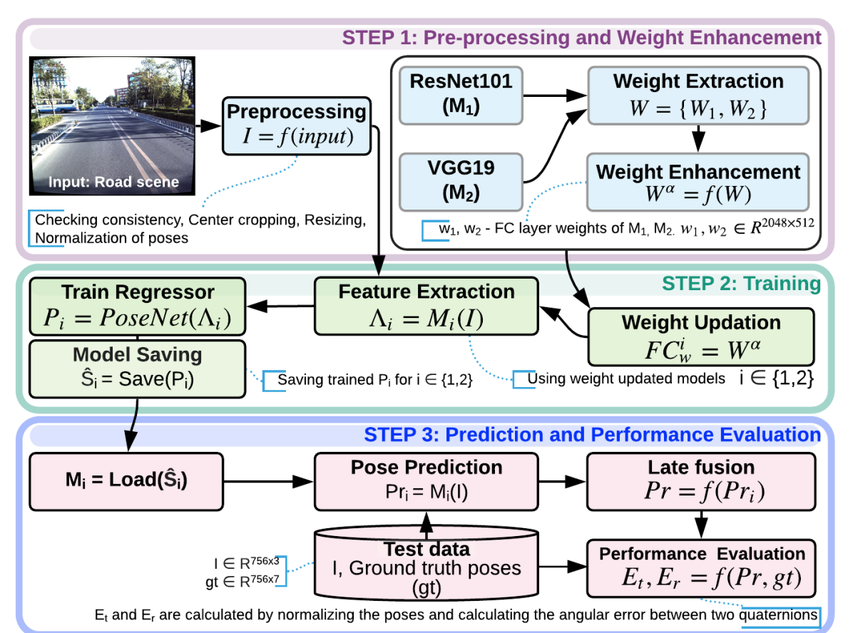
Figure 2: Operational Flow of the Proposed Hybrid Learner with a Weight Sewing Strategy and a Late Fusion Phase of the Predicted Poses Towards Improving the Localization Capability of a SLAM Model - PoseNet.

However, the hybrid learner (Fig. 2) introduced in this work is more unique and insightful than the existing hybrid fusion approaches. It focuses on enhancing and updating the weights of the pretrained unimodals before using them as front-end feature extractors of the PoseNet. Besides that it not only does a mutation of multimodal weights of the feature extraction dense layer, but also fuses the predicted scores of the pose regressor.

III PROPOSED METHOD

III-A Hybrid Weight Swing and Score Fusion Model

The Fig. 2 shows a detailed flow diagram of the hybrid learner. It consists of two parts, wherein the first part (Step 1 - weight enhancement) carries out an early fusion by layer weight enhancement of the feature extractor and the second part (Step 3) does a late fusion via score refinement of the models involved in the early fusion. The two best feature extractors chosen for early fusion based on their individual performances are used for forming the hybrid learner. The early fusion models obtained through fusing the dense layer weights of ResNet101 and VGG19 by addition or multiplication. In late fusion, the predicted scores of multiple pose regressors with the weight enhanced above feature extractors are amalgamated using average filtering to achieve better results.

III-B Preprocessing

Before passing the images and poses to the PoseNet model, it is required to preprocess the data adequately. The preprocessing involves checking the consistency of the images, resizing and center cropping of the images, extraction of mean and standard deviation, and normalization of the poses. The images are resized to $260\times 260$, and center cropped to $250\times 250$. The translation is used to get the minimum, maximum, mean and standard deviation. The rotation values are read as Euler angles which suffer from wrap around infinities, gimbal lock and interpolation problems. To overcome these challenges, Euler rotations is converted to quaternions [20].

III-C Multimodal Weight Sewing via Early Fusion (EF)

The preprocessed data is fed to the feature extractors: ResNet101 and VGG19. These two models are selected based on their individual performance on the Apolloscape test dataset. Using these two feature extractors the PoseNet has produced minimum translation and rotation errors, as recorded in Table I. The weights of the top feature extracting dense layers of the two feature extractors are fused via addition or multiplication operation. The fused values are used to update the weights of the respective dense layer of the ResNet101 and VGG19 feature extractors. The updated models are then used as new feature extractors for the regressor subnetwork. Then, the regressor is trained on the training dataset.

III-D Pose Refinement via Late Fusion (LF)

The trained models with the updated ResNet101 and VGG19 using early fusion of multiplication and addition operations are moved onto the late fusion phase as shown in Step 3 in Fig. 2. Where, the loaded weight enhanced early fusion models, simultaneously predict the poses for each input visual. The predicted scores from these models (in this case, ResNet101 and VGG19) are amalgamated with average filtering. This way of fusion is denoted as AHL. Similarly, the predicted scores of the early fusion models can be refined using multiplication and it is denoted as MHL. Finally, the predicted scores of the four early fusion models using addition and multiplication are fused together using average mathematical operation to achieve the predicted scores for the full hybrid fusion model stated earlier (Section I) in the paper as HLFF. These predicted poses are then compared with the ground truth poses to calculate the mean and median of translation and rotational errors.

IV Experimental Setup and Results

IV-A Dataset

Apolloscape dataset is used for many computer vision tasks related to autonomous driving. The Apolloscape dataset consists of modules including instance segmentation, scene parsing, lanemark parsing and self-localization that are used to understand and make a vehicle to act and reason accordingly [3, 2]. The Apolloscape dataset for self-localization is made up of images and poses on different roads at discrete locations. The images and the poses are created from the recordings of the videos. Each record of the dataset has multiple images and poses corresponding to every image. The road chosen for the ablation study of this research is zpark. It consists of a total of 3000 stereo vision road scenes. For each image, there is a ground truth of poses with 6-DoF. From this entire dataset, a mutually exclusive training and test sets are created with the ratio of $3:1$.

IV-B Evaluation Metric

Measuring the performance of the machine learning model is pivotal to comparing the various CNN models. Since every CNN model is trained and tested on different datasets with varied hyperparameters, it is necessary to choose the right evaluation metric. As the domain of this work is a regression problem, the mean absolute error (MAE) is used to measure the performance of the set of models ranging from unimodals to the proposed hybrid learner. MAE is a linear score, which is calculated as an average of the absolute difference between the target variables and the predicted variables using the formula given in Eq. (8).

$$MAE=\frac{1}{n}\sum_{i=1}^{n}\mid{x_{i}-x}\mid,$$ (8)

where, $n$ is the total number of samples in the validation dataset, $x_{i}$ and $x$ are the predicted and ground truth poses, respectively. Since, it is an average measure, it implies that all the distinct values are weighted equally ignoring any bias involvement.

Model Name	Median $\mathbf{e_{t}(m)}$	Mean $\mathbf{e_{t}(m)}$	Median $\mathbf{e_{r}(^{\circ})}$	Mean $\mathbf{e_{r}(^{\circ})}$	MAPST $\mathbf{(s)}$
M$1$ - ResNet$18$	$21.194$	$24.029$	$0.778$	$0.900$	$0.092$
M$2$ - ResNet$34$	$20.990$	$23.597$	$0.673$	$0.824$	$0.093$
M$3$ - ResNet$50$	$18.583$	$20.803$	$0.903$	$1.434$	$0.095$
M$4$ - ResNet$101$	$16.227$	$19.427$	$0.966$	$1.230$	$0.098$
M$5$ - VGG$16$	$17.150$	$21.571$	$1.079$	$1.758$	$0.103$
M$6$ - VGG$19$	$16.820$	$19.935$	$0.899$	$1.378$	$0.111$
M$7$ - AlexNet	$46.992$	$53.004$	$4.282$	$7.177$	$0.108$
M$8$ - LF	$9.763$	$10.561$	$0.945$	$4.645$	$0.146$
M$9$ - AEFResNet101	$14.870$	$18.256$	$0.673$	$0.784$	$0.134$
M$10$ - MEFResNet101	$14.842$	$18.013$	$0.779$	$0.977$	$0.131$
M$11$ - AEFVGG19	$11.047$	$13.840$	$0.742$	$1.024$	$0.137$
M$12$ - MEFVGG19	$10.730$	$14.181$	$0.756$	$1.141$	$0.135$
M$13$ - AHL	$10.400$	$12.193$	$0.828$	$5.155$	$0.142$
M$14$ - MHL	$9.307$	$11.420$	$1.206$	$5.455$	$0.142$
M$15$ - HLFF	$7.762$	$8.829$	$1.008$	$4.618$	$0.144$

TABLE I: Performance Analysis of Various Models: $e_{t}$ - translation error, $e_{r}$ - rotation error, MAPST - mean average per sample processing time.

IV-C Performance Analysis

This Section elaborates the results obtained from each of the model introduced earlier in this paper.

IV-C1 Translation and Rotation Errors

Table I tabulates the performance of the PoseNet with various front-end unimodel and multimodal feature extractors, along with the proposed hybrid learners. The results in this Table can be described in three subdivisions. The primary section from M$1$ to M$7$ is the outcomes of the unimodal PoseNet with unimodality-based feature extractors. The subsequent section extending from M$8$ to M$12$ depicts the performances of five multimodality-based learners. M$8$ represents late fusion (LF), M$9$ (AEF^ResNet101) and M$10$ (MEF^ResNet101) represent early fusion on ResNet101 as feature extractor with addition and multiplication, respectively. M$11$ (AEF^VGG19) and M$12$ (MEF^VGG19) are the results for early fusion on VGG$19$ with addition and multiplication, respectively. The third section consists of proposed hybrid learners, where M$13$, M$14$, and M$15$ stand for AHL that combines the early fusion models, M$9$ and M$11$, MHL, which combines the early fusion models, M$10$ and M$12$, and the HLFF obtained after averaging the predicted scores of the four models, M$9$, M$10$, M$11$, and M$12$. The results are computed as the mean and median values of translation and rotation errors. The translation errors are measured in terms of meters ($m$), while the rotation error is measured in degrees $(^{\circ})$.

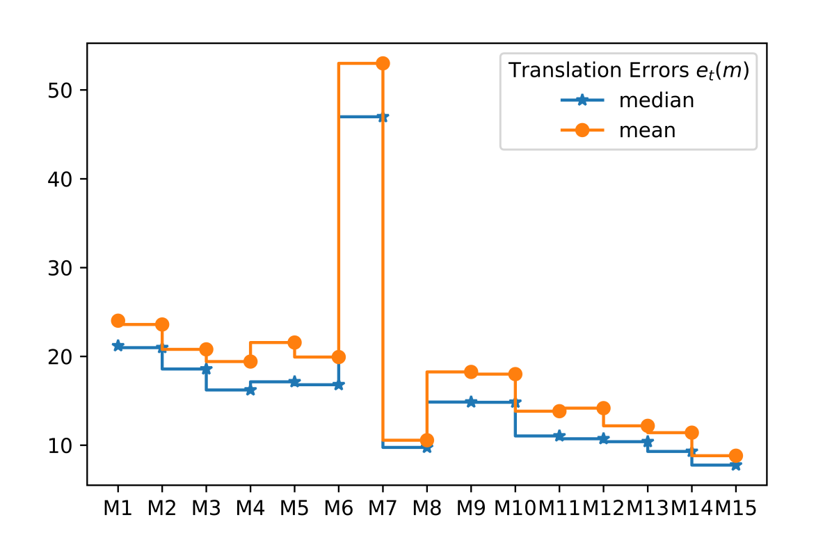
(a) Error in Terms of Translation.

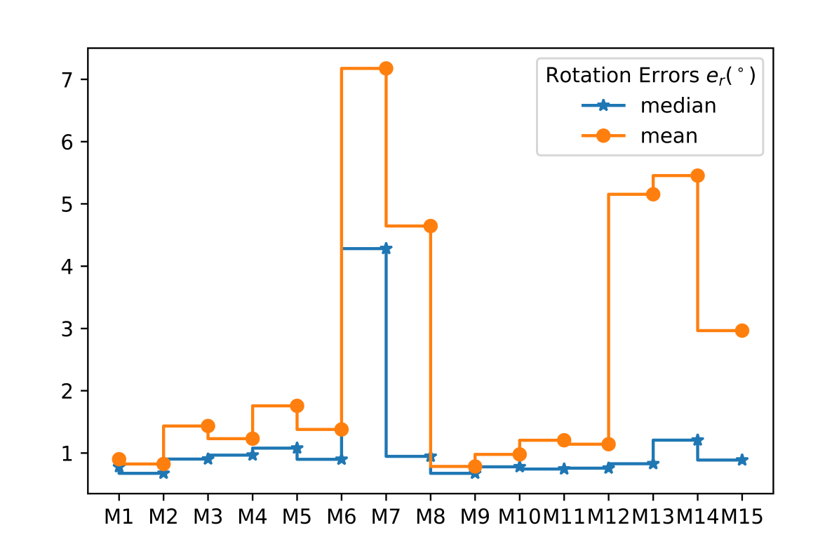
(b) Error in Terms of Rotation.

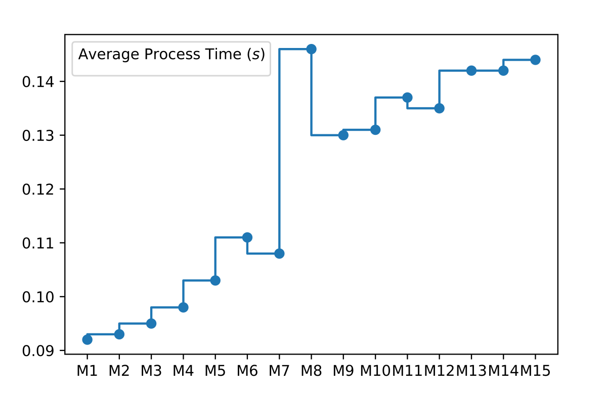
(c) Average Processing Time per Sample.

Figure 3: Performance Analysis of All Different Models.

Considering the unimodal-based PoseNet implementation, it is very apparent that ResNet$101$ and VGG$19$ give the best two outcomes among others. In terms of translation error, the late fusion model shows better performance than unimodality-based learners, but not good as compared to the early fusion model. Let’s pick the ResNet$101$-based PoseNet as baseline model for rest of the comparative analysis because it has the best performance amongst the all the unimodals. Here, the late fusion shows a $66$% decrease in the translation’s median errors and an $84$% decrease in the translation’s mean errors when compared to ResNet$101$ (M$4$). The median of rotation errors in the late fusion model shows a decrease of $2$% but the mean of rotation errors increase by $73$%.

On comparison of the baseline model (M$4$) with the early fusion model using addition having ResNet101 as a feature extractor (M$9$), it is seen that there is a $9$% decrease in translation’s median error and a $6$% decrease in translation’s mean error. On the other hand, the median of rotation error shows a $43$% decrease and mean of rotation error shows a $41$% decrease. The comparison with the early fusion model (M$10$) using multiplication on VGG$19$ exhibits a $51$% decrease in translation’s median error and a $37$% decrease in translation’s mean error. While the rotation errors drop in median value by $28$% and in the mean value by $8$%.

It is evident from the Table I that hybrid learners show much better performance than the unimodal and early fusion models. The hybrid learner using average filtering shows a $109$% decrease in the translation’s median errors and a $120$% decrease in the translation’s mean error when compared to the ResNet$101$-based PoseNet. While for rotation errors, there is a $4$% increase in the median and a $73$% increase in the mean.

In holistic analysis, it is observed that the late fusion shows an improvement of $37$% in translation and $3$% in rotation. On considering the early fusion model using ResNet as a feature extractor, the translation shows $6\%$ improvement while rotation shows $31$%. The improvement of the early fusion using VGG$19$ as a feature extractor in terms of translation and rotation is $31$% and $24$%, respectively. It is quite evident from the Table II that the proposed HL has a negligible low results for rotation with a decrease of $4$% nevertheless, it is the best model considering a huge improvement in translation by $50$% across all the modals.

Model Name	Improvement in		Timing Overhead $(ms)$
	$e_{t}$ (%)	$e_{r}$ (%)
LF	$37$	$3$	$48$
EFResNet	$6$	$31$	$36$
EFVGG	$31$	$24$	$39$
HLFF	$50$	$-4$	$46$

TABLE II: Performance Improvement of Proposed Hybrid Learner When Compared to the Baseline PoseNet with ResNet101 as Front-end.

IV-D Timing Analysis

The timing analysis is conducted on a machine that uses an Intel Core i5 processor that uses the Google Colaboratory having a GPU chip Tesla K80 with 2496 CUDA cores, a hard disk space of 319GB and 12.6GB RAM. Table I shows the mean average processing time calculated for processing a batch of ten samples.

As seen from the Table I and Figure 3, the fusion models which involve early, late, and hybrid learner take slightly extra time compared to the unimodality-based baseline PoseNet. The late fusion model (M8) takes more processing time in comparison to all the other models, as it uses five pretrained modalities, which are trained and tested individually, thereby, increasing the time overhead. The early fusion models also show an increase in the processing time in comparison to the unimodels but lesser than the late fusion model, as training the pretrained model after weight enhancement takes more time. The hybrid learners also show the same trend because of the underlying fact that it is a combination of the early and late fusion methods. These models employ weight enhanced early fusion models adding to the time overhead, besides fusing the scores from different models after validation.

Note that the hyper-parameters have been fixed throughout the experimental analysis on various models to avoid uncertainties in the comparative study. The learning rate used in all the models is $0.01$, dropout rate for the dropout layer of the PoseNet is set to $0.5$, and the batch size during training is fixed to $34$. Hence, every model is trained for $1000$ epochs with Adam optimizer.

V Conclusion

This work introduces a the hybrid learner to improve the localization accuracy of a pose regressor model for SLAM. The hybrid learner is a combination of multimodal early and late fusion algorithms to harness the best properties of the both. The extensive experiments on the Apolloscape self-localization dataset show that the proposed hybrid leaner is capable of reducing the translation error nearly by a $50$% decrease, although the rotation error gets worse by a negligible $4$% when compared to unimodal PoseNet with ResNet$101$ as a feature extractor.

Thus, the future work aims at minimizing the rotation errors and overcoming the little overhead in the processing time.

References

- [1] A. Kendall, M. Grimes, and R. Cipolla, “Posenet: A convolutional network for real-time 6-dof camera relocalization,” in Proceedings of the IEEE international conference on computer vision, pp. 2938–2946, 2015.
- [2] P. Wang, R. Yang, B. Cao, W. Xu, and Y. Lin, “Dels-3d: Deep localization and segmentation with a 3d semantic map,” in CVPR, pp. 5860–5869, 2018.
- [3] P. Wang, X. Huang, X. Cheng, D. Zhou, Q. Geng, and R. Yang, “The apolloscape open dataset for autonomous driving and its application,” IEEE transactions on pattern analysis and machine intelligence, 2019.
- [4] T. Bailey and H. Durrant-Whyte, “Simultaneous localization and mapping (slam): Part ii,” IEEE robotics & automation magazine, vol. 13, no. 3, pp. 108–117, 2006.
- [5] M. Montemerlo, S. Thrun, D. Koller, B. Wegbreit, et al., “Fastslam 2.0: An improved particle filtering algorithm for simultaneous localization and mapping that provably converges,” in IJCAI, pp. 1151–1156, 2003.
- [6] M. Montemerlo, S. Thrun, D. Koller, B. Wegbreit, et al., “Fastslam: A factored solution to the simultaneous localization and mapping problem,” Aaai/iaai, vol. 593598, 2002.
- [7] R. C. Smith and P. Cheeseman, “On the representation and estimation of spatial uncertainty,” The international journal of Robotics Research, vol. 5, no. 4, pp. 56–68, 1986.
- [8] F. Walch, C. Hazirbas, L. Leal-Taixé, T. Sattler, S. Hilsenbeck, and D. Cremers, “Image-based localization with spatial lstms,” CoRR, vol. abs/1611.07890, 2016.
- [9] A. Kendall and R. Cipolla, “Geometric loss functions for camera pose regression with deep learning,” in Proceedings of the IEEE Conference on Computer Vision and Pattern Recognition, pp. 5974–5983, 2017.
- [10] M. E. Taylor and P. Stone, “Transfer learning for reinforcement learning domains: A survey,” Journal of Machine Learning Research, vol. 10, no. Jul, pp. 1633–1685, 2009.
- [11] A. Krizhevsky, I. Sutskever, and G. E. Hinton, “Imagenet classification with deep convolutional neural networks,” in Advances in neural information processing systems, pp. 1097–1105, 2012.
- [12] K. Simonyan and A. Zisserman, “Very deep convolutional neural networks for large-scale image recognition,” in The International Conference on Learning Representations, 2015, pp. 1–5, 2015.
- [13] R. S. Paolo Napoletano, Flavio Piccoli, “Anomaly detection in nanofibrous materials by cnn-based similarity,” MDPI, 2018.
- [14] J. Xu, Y. Zhao, J. Jiang, Y. Dou, Z. Liu, and K. Chen, “Fusion model based on convolutional neural networks with two features for acoustic scene classification,” in Proc. of the Detection and Classification of Acoustic Scenes and Events 2017 Workshop (DCASE2017), Munich, Germany, 2017.
- [15] T. Akilan, Q. M. J. Wu, and H. Zhang, “Effect of fusing features from multiple dcnn architectures in image classification,” The Institution of Engineering and Technology, Feb 2018.
- [16] Y. Fu, L. Cao, G. Guo, and T. S. Huang, “Multiple feature fusion by subspace learning,” in Proceedings of the 2008 international conference on Content-based image and video retrieval, pp. 127–134, 2008.
- [17] S. Bahrampour, N. Nasrabadi, A. Ray, and W. Jenkins, “Multimodal task-driven dictionary learning for image classification,” The IEEE Transactions on Image Processing, 2015.
- [18] Y. Sun, X. Wang, and X. Tang, “Hybrid deep learning for face verification,” in Proceedings of the IEEE international conference on computer vision, pp. 1489–1496, 2013.
- [19] V. Pawar and S. Talbar, “Hybrid machine learning approach for object recognition: Fusion of features and decisions,” Machine Graphics and Vision, vol. 19, no. 4, pp. 411–428, 2010.
- [20] P. Bouthellier, “Rotations and orientations in r3,” 27th International Conference on Technology in Collegiate Mathematics, vol. 27, 2015.