Using Mars co-orbitals to estimate the importance of rotation-induced YORP break-up events in Earth co-orbital space

Abstract

Both Earth and Mars host populations of co-orbital minor bodies. A large number of present-day Mars co-orbitals is probably associated with the fission of the parent body of Mars Trojan 5261 Eureka (1990 MB) during a rotation-induced Yarkovsky–O’Keefe–Radzievskii–Paddack (YORP) break-up event. Here, we use the statistical distributions of the Tisserand parameter and the relative mean longitude of Mars co-orbitals with eccentricity below 0.2 to estimate the importance of rotation-induced YORP break-up events in Martian co-orbital space. Machine-learning techniques ($k$-means++ and agglomerative hierarchical clustering algorithms) are applied to assess our findings. Our statistical analysis identified three new Mars Trojans: 2009 SE, 2018 EC₄ and 2018 FC₄. Two of them, 2018 EC₄ and 2018 FC₄, are probably linked to Eureka but we argue that 2009 SE may have been captured, so it is not related to Eureka. We also suggest that 2020 VT₁, a recent discovery, is a transient Martian co-orbital of the horseshoe type. When applied to Earth co-orbital candidates with eccentricity below 0.2, our approach led us to identify some clustering, perhaps linked to fission events. The cluster with most members could be associated with Earth quasi-satellite 469219 Kamo‘oalewa (2016 HO₃) that is a fast rotator. Our statistical analysis identified two new Earth co-orbitals: 2020 PN₁, which follows a horseshoe path, and 2020 PP₁, a quasi-satellite that is dynamically similar to Kamo‘oalewa. For both Mars and Earth co-orbitals, we found pairs of objects whose values of the Tisserand parameter differ by very small amounts, perhaps hinting at recent disruption events. Clustering algorithms and numerical simulations both suggest that 2020 KZ₂ and Kamo‘oalewa could be related.

1 Introduction

Asteroids can split into two or more components due to the effect of solar-radiation-driven forces on their spin rate. The Yarkovsky–O’Keefe–Radzievskii–Paddack (YORP) mechanism (see e.g. Bottke et al. 2006) can secularly increase the rotation rate of asteroids and make them reach the critical fission frequency, triggering break-up events (Walsh, Richardson & Michel, 2008) that may lead to the formation of unbound asteroid pairs (Vokrouhlický & Nesvorný, 2008; Pravec et al., 2010; Jacobson & Scheeres, 2011; Scheeres, 2018; Pravec et al., 2019) and clusters (Pravec et al., 2018; Carruba, Ramos & Spoto, 2020; Carruba et al., 2020a; Fatka, Pravec & Vokrouhlický, 2020).

Mars hosts a group of Trojan asteroids that may have formed during a rotation-induced YORP break-up event (Christou et al., 2020). The so-called Eureka cluster or family – after its largest member 5261 Eureka (1990 MB), which is a 2-km binary asteroid – includes at least nine members (Christou et al., 2020), see Table 1. Spectroscopic analysis has shown that some members of this cluster exhibit a distinctive olivine-dominated composition that lends further support to the common origin scenario (Borisov et al., 2017). On the other hand, most known Mars Trojans are believed to be primordial objects that may have remained in their current dynamical state since Mars was formed (Christou, 2013; de la Fuente Marcos & de la Fuente Marcos, 2013a; Christou et al., 2017). The stability of Mars Trojans in general and of relevant known objects in particular has been studied by e.g. Mikkola & Innanen (1994), Scholl, Marzari & Tricarico (2005), and Schwarz & Dvorak (2012). Different strategies to find more Mars Trojans have been discussed by e.g. Todd et al. (2012b, 2014).

Although so far only one Earth Trojan has been discovered, 2010 TK₇ (Connors, Wiegert & Veillet, 2011), and it is not long-term stable due to its chaotic orbit (see e.g. Dvorak, Lhotka & Zhou 2012; Zhou et al. 2019), there are dozens of known near-Earth asteroids (NEAs) that move co-orbital to our planet. Strategies to discover additional Earth co-orbitals have been discussed by e.g. Todd et al. (2012a). On the other hand, a number of NEA pairs are suspected to come from YORP-induced rotational fissions (de la Fuente Marcos & de la Fuente Marcos, 2019; Moskovitz et al., 2019) and Earth co-orbitals may also be experiencing these processes (see e.g. de la Fuente Marcos & de la Fuente Marcos 2018a). Here, we use the statistical distributions of the Tisserand parameter and the relative mean longitude of Mars co-orbitals to estimate the importance of YORP break-up events in Martian co-orbital space, then we apply the same method to study a group of objects co-orbital to Earth. This paper is organized as follows. In Section 2, we discuss data and methods. The analysis of Mars co-orbitals is presented in Section 3. Section 4 focuses on Earth co-orbitals. Machine-learning techniques are applied in Section 5 to evaluate the significance of our findings. Our results are discussed in Section 6 and our conclusions are summarized in Section 7.

Table 1: Tisserand parameter with respect to Mars, $T_{\rm Mars}$, and relative mean longitude, $\lambda_{\rm r}$, for Eureka and confirmed family members with ${\Delta}T_{\rm Mars}$ relative to Eureka included. Data are referred to epoch 2459000.5, 31-May-2020 00:00:00.0 TDB (J2000.0 ecliptic and equinox). Source: JPL’s SBDB.

Object	$T_{\rm Mars}$	$\lambda_{\rm r}$ (°)	${\Delta}T_{\rm Mars}$
5261 Eureka (1990 MB)	2.872035959	$-$57.98691	–
311999 (2007 NS2)	2.892520748	$-$55.03168	0.020484788
385250 (2001 DH47)	2.820265267	$-$56.66416	0.051770692
2011 SC191	2.892095964	$-$68.63854	0.020060004
2011 SL25	2.848673098	$-$65.67817	0.023362862
2011 SP189	2.879069290	$-$68.85747	0.007033331
2011 UB256	2.818159354	$-$55.40139	0.053876606
2011 UN63	2.871098466	$-$53.84016	0.000937494
2016 CP31	2.836038634	$-$56.61722	0.035997325

2 Data and methods

Here, we use publicly available data from Jet Propulsion Laboratory’s (JPL) Small-Body Database (SBDB) and HORIZONS on-line solar system data and ephemeris computation service, both provided by the Solar System Dynamics Group (Giorgini, 2011, 2015). The data are referred to epoch 2459000.5 Barycentric Dynamical Time (TDB) and any computed parameters are referred to the same epoch, that is also the origin of time in the calculations. Data as of 2020 December 20 have been retrieved from JPL’s SBDB and HORIZONS using tools provided by the Python package Astroquery (Ginsburg et al., 2019). Here, we focus on two groups of asteroids, co-orbitals of Mars and those of Earth with eccentricity $e<0.2$, and on the Tisserand parameter (Tisserand, 1896; Murray & Dermott, 1999). In the following, we summarize some concepts that will be used later to shape our analysis.

Co-orbital minor bodies are trapped in the 1:1 mean-motion resonance with a planet; therefore, they go around the Sun in almost exactly one planetary orbital period. Although their orbits resemble that of their host planet in terms of orbital period, they could be very eccentric and/or inclined (Morais & Morbidelli, 2002). The key parameter to classify co-orbitals is the value of the relative mean longitude, which is the difference between the mean longitude of the minor body (asteroid or comet) and that of its host planet. The mean longitude is given by $\lambda=\Omega+\omega+M$, where $\Omega$ is the longitude of the ascending node, $\omega$ is the argument of perihelion, and $M$ is the mean anomaly. Therefore, the critical angle is $\lambda_{\rm r}=\lambda-\lambda_{\rm P}$. If the value of $\lambda_{\rm r}$ oscillates over time about 0°, the object is a quasi-satellite (or retrograde satellite, although it is not gravitationally bound) to the planet (see e.g. Mikkola et al. 2006; Sidorenko et al. 2014), if it librates around 60°, the object is called an L₄ Trojan and leads the planet in its orbit, when it librates around $-$60° (or 300°), it is an L₅ Trojan and it trails the planet, if the libration amplitude is wider than 180°, the minor body follows a horseshoe path (see e.g. Murray & Dermott 1999). The Eureka cluster occupies the West Lagrange point or L₅ with respect to Mars (that moves around the Sun in a direct or eastward direction). Hybrids of these elementary co-orbital configurations are possible (Namouni, Christou & Murray, 1999; Namouni & Murray, 2000), as well as transitions between the various co-orbital states (Namouni, 1999; Namouni & Murray, 2000), elementary or hybrid. Trojans can jump from librating around L₄ to librating around L₅ and vice versa (see e.g. Tsiganis, Dvorak & Pilat-Lohinger 2000; Connors et al. 2011; Sidorenko 2018). If $\lambda_{\rm r}$ does not oscillate around a certain value, we have a passing object whose position relative to the host planet is not controlled by the 1:1 mean-motion resonance (Christou & Murray, 1999).

Numerical simulations are required to confirm any putative resonant behaviour because, sometimes, an object may seem co-orbital in terms of orbital period, but $\lambda_{\rm r}$ does not librate with time. If necessary to confirm the behaviour of $\lambda_{\rm r}$, full $N$-body calculations have been carried out as described by de la Fuente Marcos & de la Fuente Marcos (2012) using software developed by Aarseth (2003) that implements the Hermite integration scheme described by Makino (1991). The physical model includes the perturbations from the eight major planets, the Moon, the barycentre of the Pluto-Charon system, and the three largest asteroids. When integrating the equations of motion, non-gravitational forces, relativistic or oblateness terms are not taken into account. Relativistic terms can be safely neglected for orbits like the ones discussed here (see e.g. Benitez & Gallardo 2008) and the same can be said about the oblateness terms (see e.g. Dmitriev, Lupovka & Gritsevich 2015).

Tisserand’s criterion (Tisserand, 1896) is often applied to decide if two orbits computed at different epochs may perhaps belong to the same minor body; in order to apply this criterion, the object must interact directly with a single planet that must follow a low-eccentricity orbit. Assuming that the subsystem Sun-planet-minor-body can be approximated by a circular restricted three-body problem, Jacobi’s integral should be a quasi-invariant (see the discussion at the beginning of Section 6). In this case, the integral can be written as the Tisserand parameter:

$$T_{\rm P}=\frac{a}{a_{\rm P}}+2\ \cos{i}\ \sqrt{\frac{a_{\rm P}}{a}\ (1-e^{2})}\,,$$ (1)

where $a$, $e$, and $i$ are the semimajor axis, eccentricity and inclination of the orbit of the minor body, and $a_{\rm P}$ is the semimajor axis of the planet (Murray & Dermott, 1999). Our initial hypothesis is that two co-orbital (to a certain planet) minor bodies resulting from a YORP break-up event (or any less-than-gentle disruption episode for that matter) should have approximately the same values of $T_{\rm P}$, particularly if the split took place relatively recently. Co-orbital bodies with moderate values of $e$ only experience relatively distant flybys with their host planet and if the planet follows a nearly circular path, the scenario originally envisioned by Tisserand is fulfilled. This situation is found for Mars co-orbitals and those of Earth with $e<0.2$. We would like to emphasize that the functional form of equation (1) makes it robust against large uncertainties of the orbital parameters, which helps its application to objects with relatively poor orbit determinations.

Later on, we will study the distributions of $\lambda_{\rm r}$ and $T_{\rm P}$. In order to analyse the results, we produce histograms using the Matplotlib library (Hunter, 2007) with sets of bins computed using NumPy (van der Walt, Colbert & Varoquaux, 2011) by applying the Freedman and Diaconis rule (Freedman & Diaconis, 1981); instead of using frequency-based histograms, we consider counts to form a probability density so the area under the histogram will sum to one. A critical assessment of our results will be performed in Section 5 by comparing our findings with those derived from the application of machine-learning techniques provided by the Python libraries Scikit-learn (Pedregosa et al., 2011; Buitinck et al., 2013) and SciPy (Virtanen et al., 2020).

3 Mars co-orbitals

Mars’ co-orbital zone goes in terms of semimajor axis from $\sim$1.51645 au to $\sim$1.53095 au (see e.g. Connors et al. 2005). Using this constraint and considering that $e<0.2$, we have retrieved data for 44 objects from JPL’s SBDB, and computed $\lambda_{\rm r}$ and $T_{\rm Mars}$ referred to epoch 2459000.5 for each one of them.

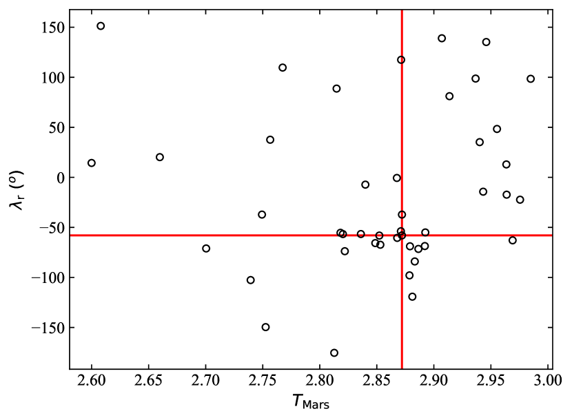
Figure 1: Distribution of relative mean longitudes, $\lambda_{\rm r}$, as a function of the Tisserand parameter, $T_{\rm Mars}$, for Mars co-orbital candidates (44 objects). The red lines mark the values for 5261 Eureka (1990 MB).

Results are plotted in Fig. 1; the red lines mark the values for 5261 Eureka (1990 MB) that is the main object of the cluster mentioned in Section 1. The values of $\lambda_{\rm r}$ and $T_{\rm Mars}$ for the members of the cluster discussed by Christou et al. (2020) are given in Table 1. Following Christou et al. (2020), we will assume that these objects are the result of one or more YORP break-up events. The absolute value of the difference between the value of $T_{\rm Mars}$ for the object and that of Eureka is shown in Table 1 as ${\Delta}T_{\rm Mars}$. From these values, we find that ${\Delta}T_{\rm Mars}<0.054$ could be compatible with a common origin under the assumptions made. On the other hand, we have that the Martian Trojan with the value of the Tisserand parameter closest to that of Eureka is 2011 UN₆₃ followed by 2011 SP₁₈₉ (see Table 1).

In Fig. 1, we observe that there is a conspicuous cluster of objects around the position of Eureka; there is no symmetrical cluster in the expected position of the L₄ Trojan cloud, which is consistent with previous findings (Borisov et al., 2018; Christou et al., 2020). Either the event that led to the formation of the Eureka family was exclusive to L₅ or there is a process that has been able to remove most objects from L₄ (see the analysis in Christou et al. 2020). In addition, we observe in Fig. 1 that two objects have very low values of ${\Delta}T_{\rm Mars}$ with respect to Eureka although they cannot be part of the L₅ Trojan cloud. The lowest is found for 2001 FG₂₄ with ${\Delta}T_{\rm Mars}=0.0000060$ and $\lambda_{\rm r}=-37\aas@@fstack{\circ}21$, that is not currently engaged in resonant behaviour, but simulations (not shown) reveal that it may have been a transient horseshoe librator in the past and this situation may repeat in the future; the second lowest is 490718 (2010 RL₈₂) with ${\Delta}T_{\rm Mars}=0.0007294$ and $\lambda_{\rm r}=117\aas@@fstack{\circ}45$, that shares dynamical status with 2001 FG₂₄ (their mutual ${\Delta}T_{\rm Mars}$ is 0.0007354). Fragments may leave the Trojan clouds via Yarkovsky-driven orbital evolution as discussed by Scholl et al. (2005), Ćuk, Christou & Hamilton (2015), and Christou et al. (2020). In general, asteroid families may evolve through a combination of YORP, Yarkovsky, and collisional events (see e.g. Marzari et al. 2020). Two objects from Table 1, 311999 (2007 NS₂) and 2011 SC₁₉₁, also have a very low mutual ${\Delta}T_{\rm Mars}$, 0.0004248.

Considering the boundaries defined by the data in Table 1 – i.e. ${\Delta}T_{\rm Mars}<0.054$ with respect to Eureka and $\lambda_{\rm r}\in(-68\aas@@fstack{\circ}9,-53\aas@@fstack{\circ}8)$, the locus of the Eureka cluster in the $T_{\rm Mars}$–$\lambda_{\rm r}$ plane – at least 12 known Martian co-orbitals, including Eureka, could be Eureka family members (see Fig. 2). The three new L₅ Trojans – 2009 SE, 2018 EC₄ and 2018 FC₄ – are shown in Table 2 and their status is confirmed in Fig. 3, top panel (but see the more detailed analysis in Section 6.1). These three objects can be regarded as robust L₅ Trojans and perhaps members of the Eureka family (but see Section 6.1). Outside the locus of the cluster, we find 2020 VT₁, a recent discovery that has $\lambda_{\rm r}=-0\aas@@fstack{\circ}5983$ (but it is not a quasi-satellite, see Fig. 3, bottom panel) and ${\Delta}T_{\rm Mars}$ relative to Eureka of 0.0044492 (see Section 6.1 for additional details).

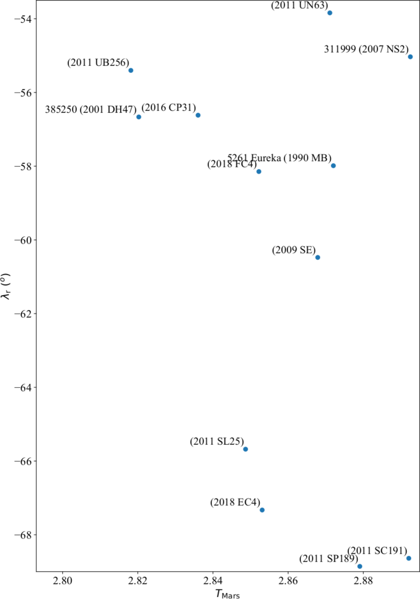
Figure 2: Relative positions in the $T_{\rm Mars}$-$\lambda_{\rm r}$ plane of the objects in Tables 1 and 2. No objects have been removed from the displayed region, i.e. no known interlopers are present in the area of the $T_{\rm Mars}$-$\lambda_{\rm r}$ plane occupied by Mars’ L₅ Trojan cloud.

Table 2: As Table 1 but for new Eureka family member candidates within the locus discussed in the text. The last column gives the data-arc in days.

Object	$T_{\rm Mars}$	$\lambda_{\rm r}$ (°)	${\Delta}T_{\rm Mars}$	arc (d)
2009 SE	2.867875826	$-$60.47576	0.004160134	3133
2018 EC4	2.853092552	$-$67.32835	0.018943407	3131
2018 FC4	2.852214411	$-$58.14554	0.019821549	790

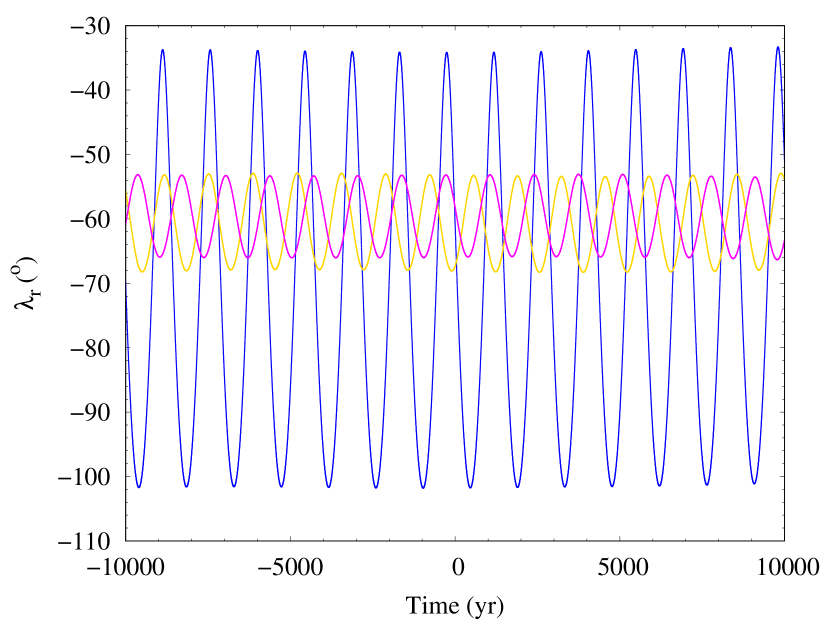
Figure 3: Evolution of the mean longitude difference of 2009 SE (blue), 2018 EC₄ (gold) and 2018 FC₄ (magenta) and Mars (top panel), and that of 2020 VT₁ (bottom panel). The output time-step size is 1 yr, the origin of time is epoch 2459000.5 TDB, and only nominal orbits have been displayed (see Section 6.1 for a detailed discussion).

In order to investigate the statistical significance of our results regarding ${\Delta}T_{\rm Mars}$, we have computed the mutual differences between the values of $T_{\rm Mars}$ for all the objects in our sample. The resulting histogram is shown in Fig. 4. The mean value and standard deviation are 0.10$\pm$0.08; the median and 16th and 84th percentiles are 0.08${}_{-0.06}^{+0.11}$. Although the distributions are not normal, in a normal distribution a value that is one standard deviation above the mean is equivalent to the 84th percentile and a value that is one standard deviation below the mean is equivalent to the 16th percentile (see e.g. Wall & Jenkins 2012). By providing these values (standard deviation and the relevant percentiles), we wanted to quantify how non-normal the distribution is.

The distribution in Fig. 4 shows that the probability of having two objects with ${\Delta}T_{\rm Mars}<0.054$ is, $P(<0.054)=0.3404$; we also have $P(<0.005)=0.0402$ and $P(<0.0001)=0.0011$. Therefore, the case of Eureka and 2001 FG₂₄ pointed out above is indeed unusual. In terms of probability, it may be possible that 2001 FG₂₄ (that has a data-arc of 7119 d) was part of Eureka (a fast rotator) in the past. However, this cannot have happened in the recent past because we have performed extensive calculations backwards in time for these two objects during 10⁴ yr and their closest flyby might have been at about 0.008 au. Similar calculations for the pair Eureka–2011 UN₆₃ give a distance of closest approach of 0.0008 au with a relative velocity of 3.5 km s^-1. These values are not typical of pairs resulting from a rotation-induced YORP break-up event (see e.g. Pravec et al. 2010). On the other hand, every object in our sample of 44 has at least one other object with mutual ${\Delta}T_{\rm Mars}<0.054$. The fact that no known interlopers are present in the area of the $T_{\rm Mars}$-$\lambda_{\rm r}$ plane occupied by Mars’ L₅ Trojan cloud in Fig. 2 gives some support to using this plane to find groups of minor bodies that may be related.

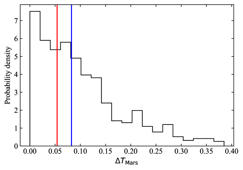
Figure 4: Distribution of ${\Delta}T_{\rm Mars}$ for all pairs of objects in our sample of Mars co-orbitals. The median value is shown in blue and the critical value of 0.054 mentioned in the text is shown in red.

4 Earth co-orbitals

Earth’s co-orbital zone goes from $\sim$0.994 au to $\sim$1.006 au (see e.g. de la Fuente Marcos & de la Fuente Marcos 2018a). Using this constraint and considering that $e<0.2$, we have retrieved data for 33 objects from JPL’s SBDB, and computed $\lambda_{\rm r}$ and $T_{\rm Earth}$ as we did in Section 3 in the case of Mars and its co-orbitals. Figure 5 shows the resulting distribution and some conspicuous clustering similar to the one present in Fig. 1 is clearly visible, but now groups appear concentrated towards $\lambda_{\rm r}\sim 0$°. When we computed the mutual differences between the values of $T_{\rm Earth}$, ${\Delta}T_{\rm Earth}$, for all the objects in our sample to investigate the statistical significance of the groupings, we obtained the histogram in Fig. 6. Now the median and 16th and 84th percentiles are 0.05${}_{-0.04}^{+0.11}$ that is below the threshold of 0.054 found in Section 3 (mean and standard deviation, 0.08$\pm$0.08). The values of the probabilities analogues to those computed in Section 3 are: $P(<0.054)=0.5644$, $P(<0.005)=0.0871$ and $P(<0.0001)=0.0019$.

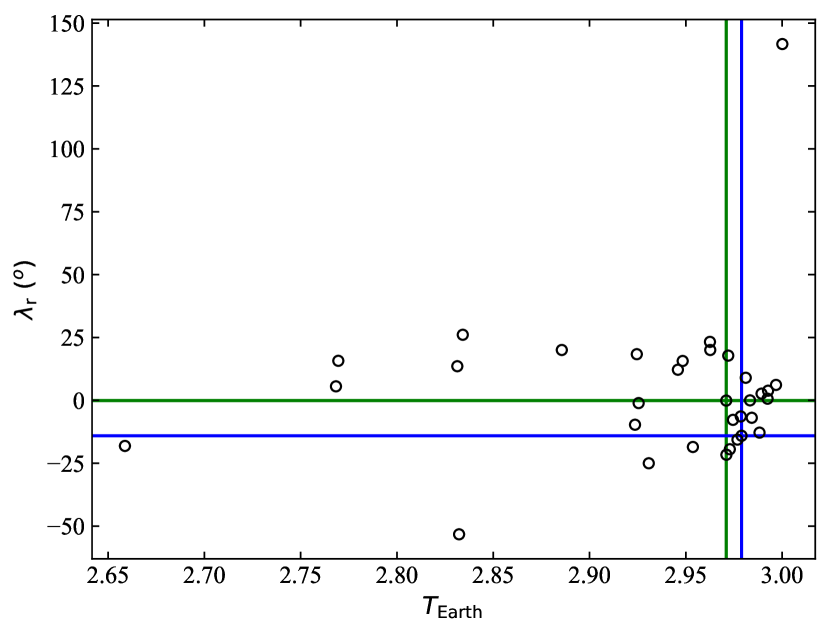
Figure 5: Distribution of relative mean longitudes, $\lambda_{\rm r}$, as a function of the Tisserand parameter, $T_{\rm Earth}$, for Earth co-orbital candidates (33 objects). The green lines mark the values for Earth quasi-satellite 469219 Kamo‘oalewa and the blue ones those of 478784 (2012 UV₁₃₆).

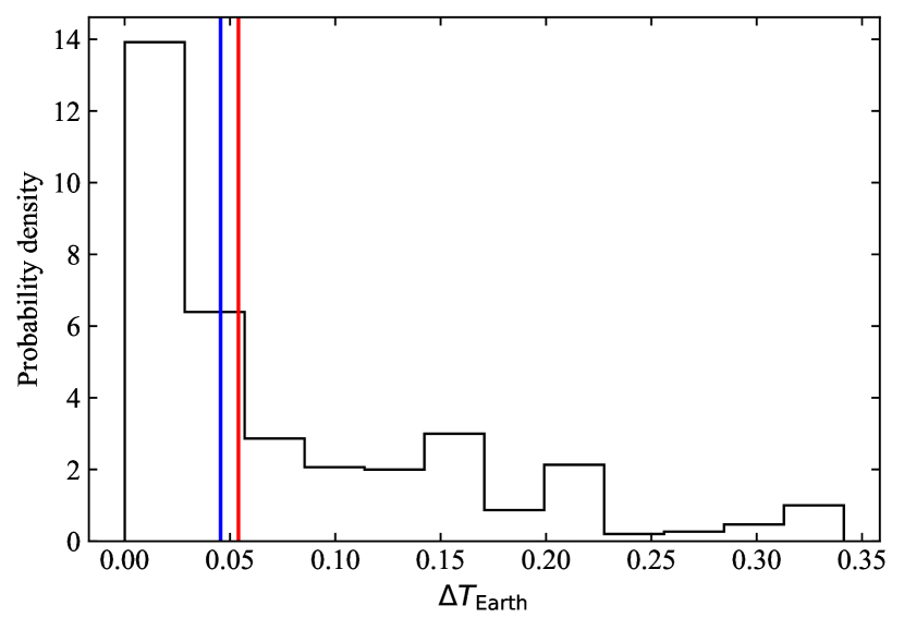
Figure 6: Distribution of ${\Delta}T_{\rm Earth}$ for all pairs of objects in our sample of Earth co-orbitals. The median value is shown in blue and the critical value of 0.054 mentioned in the text is shown in red.

The smallest value of ${\Delta}T_{\rm Earth}$, 0.00008836, is found for the pair made of 469219 Kamo‘oalewa (2016 HO₃), a quasi-satellite of Earth (de la Fuente Marcos & de la Fuente Marcos, 2016c), and 2016 FU₁₂. Given the fact that Kamo‘oalewa is an extremely fast rotator with a period of 28.03 minutes (Reddy et al., 2017), it is not difficult to argue that 2016 FU₁₂ could be the by-product of a YORP break-up event that affected the quasi-satellite in relatively recent times. A concurrent simulation into the past of the nominal orbits of both objects appears to support such a scenario as shown in Fig. 7, bottom panel, where multiple overlappings can be seen. However, extensive calculations backwards in time during 10⁴ yr for these two objects show that their closest flyby may have been at about 0.0003 au or close to 45 000 km with a relative velocity of 6.2 km s^-1. The summary of our results for the recent flybys of this pair is shown in Fig. 8 that includes the outcome of 2500 simulations that take into account the uncertainties in the orbit determinations of both bodies (see Table 3). Most flybys occur when both objects are horseshoe librators, compare the bottom panels of Figs 7 and 8. From these results, it is clear that close approaches and perhaps collisions between Earth co-orbitals are possible. Putative collisions may take place at speeds (see Fig. 8, middle panel) in excess of those typical in the main asteroid belt, 6$\pm$2 km s^-1 (see e.g. Farinella & Davis 1992). As pointed out in the previous section for relevant pairs of Mars co-orbitals, these values are not typical of pairs resulting from a rotation-induced YORP break-up event (see e.g. Pravec et al. 2010).

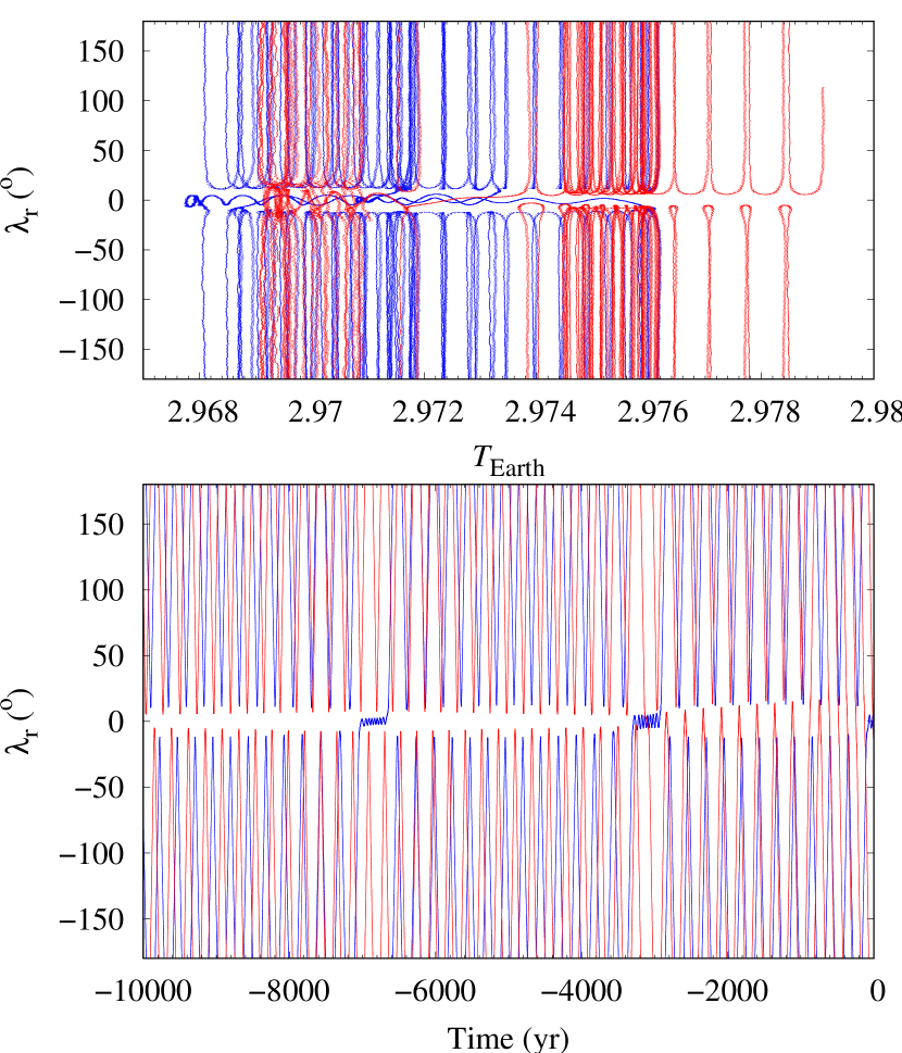
Figure 7: Concurrent past evolution over 10 000 yr of 469219 Kamo‘oalewa (in blue) and 2016 FU₁₂ (in red) in the $T_{\rm Earth}$-$\lambda_{\rm r}$ plane (top panel) and in $\lambda_{\rm r}$ (bottom panel). Kamo‘oalewa switches multiple times between the quasi-satellite and horseshoe configurations, while 2016 FU₁₂ followed an asymmetric and irregular horseshoe path. The output time-step size is 0.002 yr, the origin of time is epoch 2459000.5 TDB, and only nominal orbits have been displayed.

Table 3: Heliocentric Keplerian orbital elements of 469219 Kamo‘oalewa (2016 HO₃), 2016 FU₁₂, and 2020 KZ₂ used in this study. The orbit determination of Kamo‘oalewa is based on 307 observations spanning a data-arc of 5140 d or 14.07 yr (solution date, 2018-Apr-30 06:51:17 PDT), the one of 2016 FU₁₂ is based on 19 observations spanning a data-arc of 4 d (solution date, 2017-Apr-06 08:27:11 PDT), and that of 2020 KZ₂ is based on 39 observations spanning a data-arc of 8 d (solution date, 2020-May-29 06:07:53 PDT). Values include the 1$\sigma$ uncertainty. The orbit determinations have been computed at epoch JD 2459000.5 that corresponds to 00:00:00.000 TDB on 2020 May 31 (J2000.0 ecliptic and equinox). Source: JPL’s SBDB.

Orbital parameter		469219 Kamo‘oalewa	2016 FU12	2020 KZ2
Semimajor axis, $a$ (au)	=	1.001247952$\pm$0.000000003	1.0050$\pm$0.0002	1.00530$\pm$0.00003
Eccentricity, $e$	=	0.1033008$\pm$0.0000002	0.166$\pm$0.002	0.028770$\pm$0.000004
Inclination, $i$ (°)	=	7.78529$\pm$0.00002	2.12$\pm$0.02	7.231$\pm$0.011
Longitude of the ascending node, $\Omega$ (°)	=	66.15571$\pm$0.00002	224.2$\pm$0.2	64.9562$\pm$0.0010
Argument of perihelion, $\omega$ (°)	=	306.18784$\pm$0.00002	198.3$\pm$0.3	7.498$\pm$0.011
Mean anomaly, $M$ (°)	=	236.29311$\pm$0.00002	164.6$\pm$0.7	176.268$\pm$0.012
Perihelion, $q$ (au)	=	0.8978182$\pm$0.0000002	0.8384$\pm$0.0015	0.97637$\pm$0.00002
Aphelion, $Q$ (au)	=	1.104677713$\pm$0.000000003	1.1717$\pm$0.0002	1.03422$\pm$0.00003
Absolute magnitude, $H$ (mag)	=	24.3$\pm$0.5	26.9$\pm$0.5	27.7$\pm$0.4

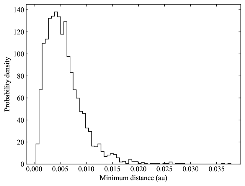
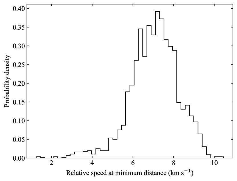
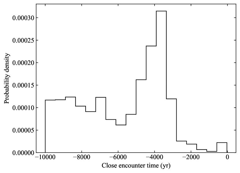
Figure 8: Distribution of minimum approach distance (top panel), relative speed at minimum distance (middle panel), and time at minimum distance (bottom panel) for calculations including 469219 Kamo‘oalewa (2016 HO₃) and 2016 FU₁₂. The origin of time in the bottom panel is epoch 2459000.5 TDB. Input values from Tables 12 and 13.

No actual collisions between asteroids have ever been observed although the outcome of several of them may have been studied: 354P/LINEAR (see e.g. Snodgrass et al. 2010), (596) Scheila (see e.g. Bodewits et al. 2011), (493) Griseldis (Tholen, Sheppard & Trujillo, 2015), and P/2016 G1 (PANSTARRS) (Moreno et al., 2016, 2017; Hainaut et al., 2019). The observed fragments resulting from these events have been produced by excavation, leading to a low launch velocity of the ejecta from the surface of the target body, a relatively large asteroid (larger than objects like Kamo‘oalewa). Numerical simulations indicate that velocities of ejecta relative to target may not be much higher than a few hundred m s^-1 and often significantly lower than that (see e.g. Appendix E in Ševeček et al. 2017 or Jutzi et al. 2010). However, we have detailed observations of at least one high-speed collision of small bodies in our immediate neighbourhood, the Iridium–Cosmos collision event. On 2009 February 10, an inactive Russian communications satellite, Cosmos 2251, collided with an active commercial communications satellite, Iridium 33, at a relative speed of nearly 10 km s^-1 (Kelso, 2009). The two artificial satellites had similar masses (Cosmos 2251, 900 kg and Iridium 33, 689 kg), their orbital planes were nearly perpendicular, and the resulting clouds of orbital debris remained at almost right angles to each other, spreading along their original paths in a short time-scale; realistic orbital evolution analyses suggest that most fragments will probably remain in orbit around Earth for decades (Kelso, 2009; Vierinen, Markkanen & Krag, 2009; Springer et al., 2010). Although the Low Earth Orbit dynamical environment and the one travelled by Earth co-orbitals are rather different and we are speaking of manufactured not natural objects, the outcome of the high-speed collision between Iridium 33 and Cosmos 2251 may teach us a valuable lesson, that catastrophic disruptions of small bodies due to high-speed impacts may create clouds of debris that may eventually lead to objects with no genetic relationship experiencing close encounters (or even impacts). There are no reasons to assume that Iridium–Cosmos collision-like events may not be happening in Earth co-orbital space where mean-motion resonances may easily lead to intersecting orbits.

Additional objects that may be related to Kamo‘oalewa are shown in Table 4 although only Kamo‘oalewa and 2016 CO₂₄₆ have robust orbits. Out of the various clusterings seen in Fig. 5, the ones with the most members are associated with Kamo‘oalewa and 478784 (2012 UV₁₃₆) that is not currently engaged in resonant behaviour (see Table 5 for additional members). The relative positions in the $T_{\rm Earth}$-$\lambda_{\rm r}$ plane of many of the objects mentioned in our discussion are shown in Fig. 9.

Table 4: Tisserand parameter with respect to Earth, $T_{\rm Earth}$, and relative mean longitude, $\lambda_{\rm r}$, for Earth quasi-satellite Kamo‘oalewa and suspected family members with ${\Delta}T_{\rm Earth}$ relative to Kamo‘oalewa included.

Object	$T_{\rm Earth}$	$\lambda_{\rm r}$ (°)	${\Delta}T_{\rm Earth}$
469219 Kamo‘oalewa (2016 HO3)	2.97098699	$-$0.08584	–
2016 CO246	2.97203544	17.79712	0.00104845
2016 FU12	2.97107535	$-$21.61721	0.00008836
2019 XH2	2.97284981	$-$19.44256	0.00186281
2020 GE1	2.97448273	$-$7.75249	0.00349574

Table 5: Similar to Table 4 but for 478784 (2012 UV₁₃₆).

Object	$T_{\rm Earth}$	$\lambda_{\rm r}$ (°)	${\Delta}T_{\rm Earth}$
478784 (2012 UV136)	2.97894830	$-$14.07993	–
2019 GM1	2.98111706	8.98722	0.00216877
2020 GE1	2.97448273	$-$7.75249	0.00446557
2020 HE5	2.97853099	$-$6.39397	0.00041731
2020 KZ2	2.98334044	$-$0.00089	0.00439214
2020 PN1	2.97681846	$-$15.61311	0.00212984

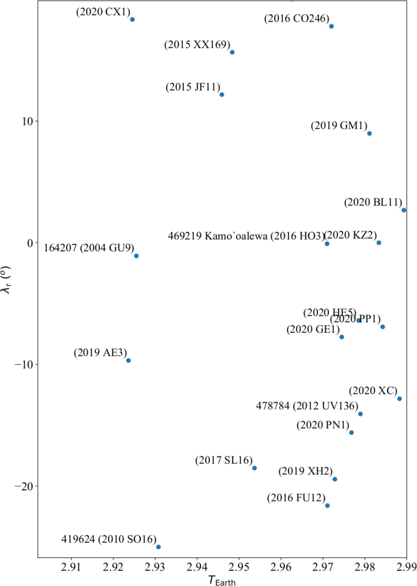
Figure 9: Relative positions of 20 Earth co-orbitals that include most of those cited in the text.

5 Clustering validation

So far, we have spoken loosely of clusterings but there are a number of statistical tools that can be used to perform such a data exploration in a rigorous way. Machine-learning techniques have sometimes been used to investigate the presence of coherent dynamical groups or genetic families within the populations of asteroids of the main belt (see e.g. Zappala et al. 1990, 1994; Masiero et al. 2013; Smirnov & Markov 2017; Carruba, Aljbaae & Lucchini 2019; McIntyre 2019; Carruba et al. 2020b). In this section, we apply unsupervised machine-learning in the form of clustering algorithms to the data discussed above. Our objective is to validate the conclusions obtained in the previous sections and perhaps extract new ones that may lead us to understand the populations of Mars and Earth co-orbitals better.

As part of the data preparation process, we have scaled the data set using standardization or Z-score normalization: found the mean and standard deviation for $T_{\rm P}$ and $\lambda_{\rm r}$, subtracted the relevant mean from each value, and then divided by its corresponding standard deviation. This was carried out by applying the method fit_transform that is part of the StandardScaler class provided by the Python library Scikit-learn (Pedregosa et al., 2011). This rescaling is strongly recommended when applying unsupervised machine-learning algorithms. Distance assignment between the objects in our sample assumes a Euclidean metric.

We have applied two different algorithms to evaluate data clustering: $k$-means++ and agglomerative hierarchical clustering. The $k$-means++ algorithm (Arthur & Vassilvitskii, 2007) performs a centroid-based analysis and it is an improved version of the $k$-means algorithm (see e.g. Steinhaus 1957; MacQueen 1967; Lloyd 1982). Here, we have used the implementation of $k$-means++ in the method fit that is part of the KMeans class provided by the Python library Scikit-learn (Pedregosa et al., 2011). On the other hand, the agglomerative hierarchical clustering algorithm (see e.g. Ward 1963) studies connectivity-based clustering aimed at building a hierarchy of clusters where each observation or data point (in our case, each object) starts as an individual cluster and clusters are merged by iteration. Here, we have used the implementation of the agglomerative hierarchical clustering algorithm included in the hierarchy module of the clustering package that is part of the Python library SciPy (Virtanen et al., 2020), specifically the functions linkage that performs hierarchical/agglomerative clustering analysis and dendrogram that plots the resulting hierarchical clustering as a dendrogram. The function linkage has been invoked using the Ward variance minimization algorithm (Ward, 1963).

For the agglomerative hierarchical clustering analysis, the dendrograms in our figures display the hierarchical merging process with the horizontal axis showing the distance at which two given clusters were merged. We have considered 0.7 of the maximal merging distance as the threshold to define the final clusters in the data set so the merging distance of objects within a cluster is significantly shorter than the merging distance of the final clusters (see additional comments below). For $k$-means++, we have used the elbow method to determine the optimal value of clusters, $k$; we invoke the method fit with $k$ in the interval (1, 10) and select the value of $k$ that minimizes the sum of the distances of all data points or objects to their respective cluster centres.

5.1 Mars co-orbitals

We have used the data set discussed in Section 3 as input to perform the clustering analyses as described above. First, we applied agglomerative hierarchical clustering to obtain the dendrogram shown in Fig. 10. The maximal merging distance is close to 8 so our threshold to define the final clusters is about 5.6 and we obtain three clusters. The top one, in red, includes all the members of the Eureka family in Table 1 and the three new Mars Trojans pointed out in Section 3. The additional L₅ Mars Trojan, 101429 (1998 VF₃₁), also appears included in this cluster, but in a different, separate branch. The L₄ Mars Trojan 121514 (1999 UJ₇) is part of a different cluster, the orange one. When applying the $k$-means++ algorithm and the elbow method to the same data set we also obtain three clusters that are shown in Fig. 11. The analysis presented in Section 3 and the one carried out here are somewhat complementary as in Section 3 we discussed one-dimensional clustering via ${\Delta}T_{\rm Mars}$ and here we consider two-dimensional clustering in the $T_{\rm Mars}$-$\lambda_{\rm r}$ plane.

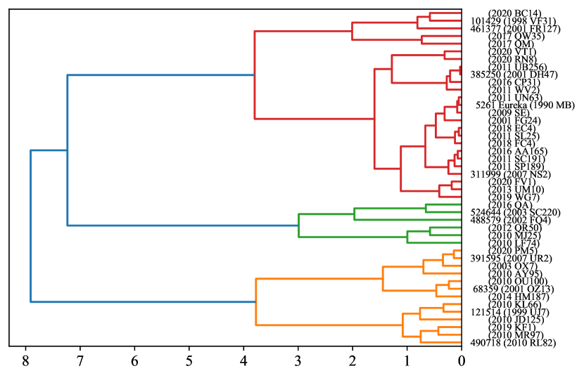
Figure 10: Dendrogram for the data set made of 44 Mars co-orbitals. The data set has been previously standardized by removing the mean and scaling to unit variance using Scikit-learn’s StandardScaler class (its method fit_transform). The $x$-axis shows the Euclidean distance between the clusters or merging distance and the $y$-axis displays the designations of the objects. This dendrogram has been computed using SciPy’s dendrogram and the Ward variance minimization algorithm of the linkage function.

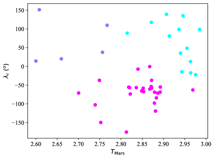
Figure 11: Colour-coded clusters generated by the $k$-means++ algorithm applied to the data set made of 44 Mars co-orbitals. The plum-coloured points correspond to the green cluster in Fig. 10, the pink points correspond to the red cluster in Fig. 10, and the cyan points belong in the orange cluster in Fig. 10.

5.2 Earth co-orbitals

Figure 12 shows the result of the application of the agglomerative hierarchical clustering to the data set discussed in Section 4. The maximal merging distance is slightly above 7 and the threshold to define the final clusters is about 5 that yields three clusters. The green one includes the vast majority of the 33 objects and both 469219 Kamo‘oalewa (2016 HO₃) and 478784 (2012 UV₁₃₆). The outlier in blue is 2006 RH₁₂₀ that is a former temporary satellite of Earth (Bressi et al., 2008; Kwiatkowski et al., 2009) with a value of $T_{\rm Earth}$ very close to 3, which means that this object follows the most Earth-like known orbit. The orange cluster includes the only known Earth Trojan, 2010 TK₇. The application of the $k$-means++ algorithm to this data set also produces three clusters that are displayed in Fig. 13. Again, the analysis presented in Section 4 and the one carried out here are somewhat complementary as in Section 4 we discussed one-dimensional clustering via ${\Delta}T_{\rm Earth}$ and here we consider two-dimensional clustering in the $T_{\rm Earth}$-$\lambda_{\rm r}$ plane.

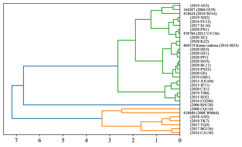
Figure 12: Same as Fig. 10 but for the data set made of 33 Earth co-orbitals.

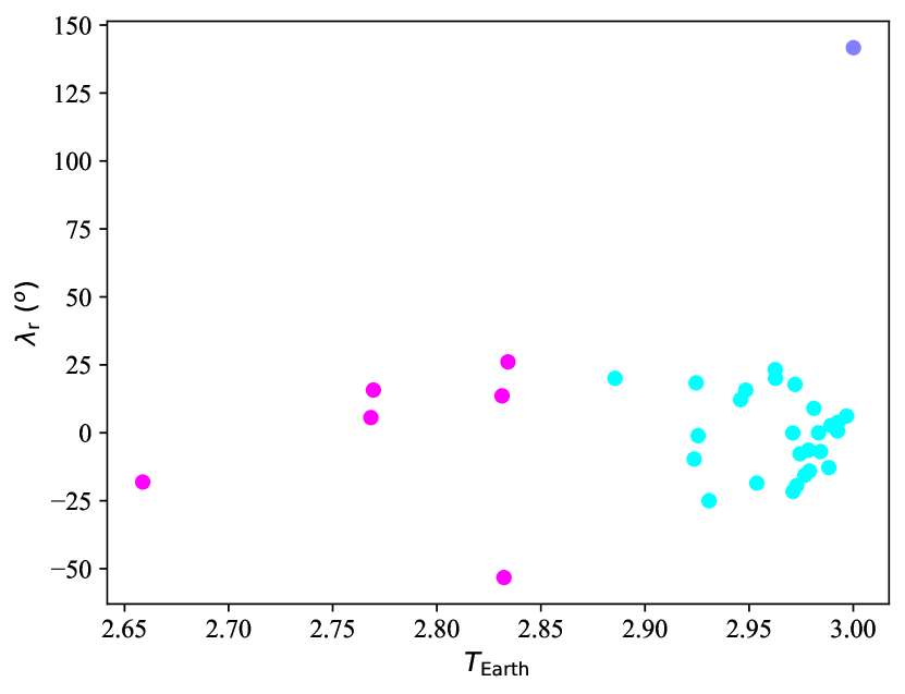
Figure 13: Same as Fig. 11 but for the data set made of 33 Earth co-orbitals. The plum-coloured point corresponds to the outlier 2006 RH₁₂₀ (see the text) that appears in blue in Fig. 12. The pink points correspond to the orange cluster in Fig. 12 that includes the only known Earth Trojan, 2010 TK₇. The cyan points are associated with the green cluster in Fig. 12.

The dendrogram in Fig. 12 indicates that the known Earth co-orbital closest to Kamo‘oalewa in the $T_{\rm Earth}$-$\lambda_{\rm r}$ plane is 2020 KZ₂. Their orbits are very similar (see Table 3, but not as similar as those discussed in de la Fuente Marcos & de la Fuente Marcos 2019) and if we perform a numerical study analogue to the one carried out for the case of Kamo‘oalewa and 2016 FU₁₂, we obtain Fig. 14 that summarizes the results of 3500 experiments. The distributions in Figs 8 and  14 are quite different. Although the orbit determinations of both 2016 FU₁₂ and 2020 KZ₂ are not as robust as that of Kamo‘oalewa (see Table 3), the inclusion of the uncertainties in the calculations reveals that 2020 KZ₂ could be a very recent fragment of Kamo‘oalewa: approaches at distances as short as 30 000 km are possible at relative velocities as low as 900 m s^-1 during the last 1000 yr. Again and as pointed out in the previous sections, these values are not typical of pairs resulting from a rotation-induced YORP break-up event (see e.g. Pravec et al. 2010). Our exploration in Section 4 suggested that 2020 KZ₂ could be related to 478784 but the agglomerative hierarchical clustering analysis carried out here and summarized in Fig. 12 together with the results of the calculations shown in Fig. 14 support a dynamical connection between Kamo‘oalewa and 2020 KZ₂. However, if they are indeed related, it is unlikely that they formed during a gentle split; a more plausible scenario may be that of two members of the population of Earth co-orbitals experiencing a collision at relatively low speed. Such a collision may initially generate two clouds of fragments moving along the original paths that eventually could spread throughout the colliding orbits. In this scenario (see also the second to last paragraph of Section 4), two fragments undergoing a flyby at a later time may have different surface properties and their relative velocity at the distance of closest approach could be close to the original impact speed as they have independent sources (the two original impactors).

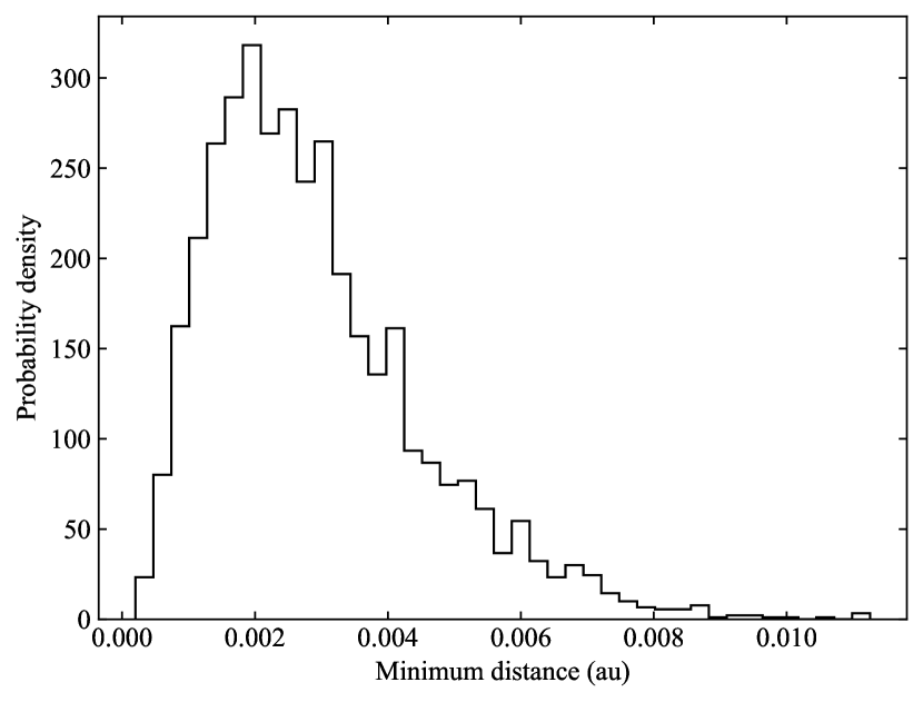
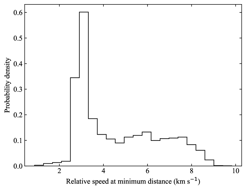
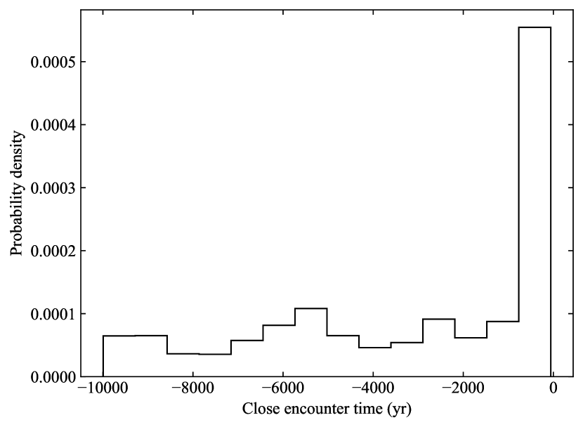
Figure 14: Distribution of minimum approach distance (top panel), relative speed at minimum distance (middle panel), and time at minimum distance (bottom panel) for calculations including 469219 Kamo‘oalewa (2016 HO₃) and 2020 KZ₂. The origin of time in the bottom panel is epoch 2459000.5 TDB. Input values from Tables 12 and 14.

6 Discussion

Our analyses follow a novel approach based on the Tisserand parameter that has seldom been used within the context of asteroid family studies, although it has a clear potential to help in a shortlisting effort. Two main objections can be made regarding this use: that the Tisserand parameter is a quasi-invariant that vary over a planetary orbital period and that we have restricted somewhat arbitrarily the application to objects with $e<0.2$. In order to understand better the implications of these objections, we have used the orbit of 5261 Eureka (1990 MB) as a test case and integrated its nominal orbit for 10⁵ yr forward in time together with five other orbits similar to that of Eureka but with $e=0.0$, 0.1, 0.2, 0.3, 0.4 and 0.5 (Eureka has $e=0.065$). The results of these integrations are displayed, in the $T_{\rm Mars}$-$\lambda_{\rm r}$ plane, in Fig. 15. The top panel of the figure shows that an originally confined path becomes unconfined as the value of the eccentricity increases, supporting our choice of $e<0.2$ to select relevant objects. The Tisserand parameter is relevant to the circular restricted three-body problem that is an idealized situation in which the Sun, a planet, and a massless body interact. Therefore, it assumes that the dynamics of the massless body is not significantly influenced by a fourth body. This is very nearly the case of Mars co-orbitals with $e<0.2$, but Earth co-orbitals evolve within the dynamical context of the Earth-Moon system although few known objects seem to be significantly affected by the Moon (see below).

The issue of the quasi-invariant nature of the Tisserand parameter becomes clear when considering the bottom panel of Fig. 15: although the osculating value (the one displayed) changes over time, the average value remains reasonably constant over extended periods of time. The oscillations observed are the result of secular perturbations driven by planets other than Mars: the eccentricity fluctuates with a periodicity of about 200 000 yr and the inclination oscillates on a time-scale of 600 000 yr (Mikkola et al., 1994). Its eccentricity oscillates mainly due to secular resonances with the Earth and the oscillation in inclination appears to be driven by secular resonances with Jupiter (see e.g. de la Fuente Marcos & de la Fuente Marcos 2013a). Figure 15, bottom panel, provides a good context to understand the clusterings discussed in the previous sections: any co-orbital body that splits tends to have its resulting fragments confined within short distance in the $T_{\rm P}$-$\lambda_{\rm r}$ plane. It is however possible that a similar arrangement may arise from a purely dynamical mechanism, without any fragmentation involved, but it probably requires a very large source population, large enough to facilitate the process of capture inside the co-orbital resonance with very similar values of $T_{\rm P}$ that have very low intrinsic probabilities (see the values in Sections 3 and 4).

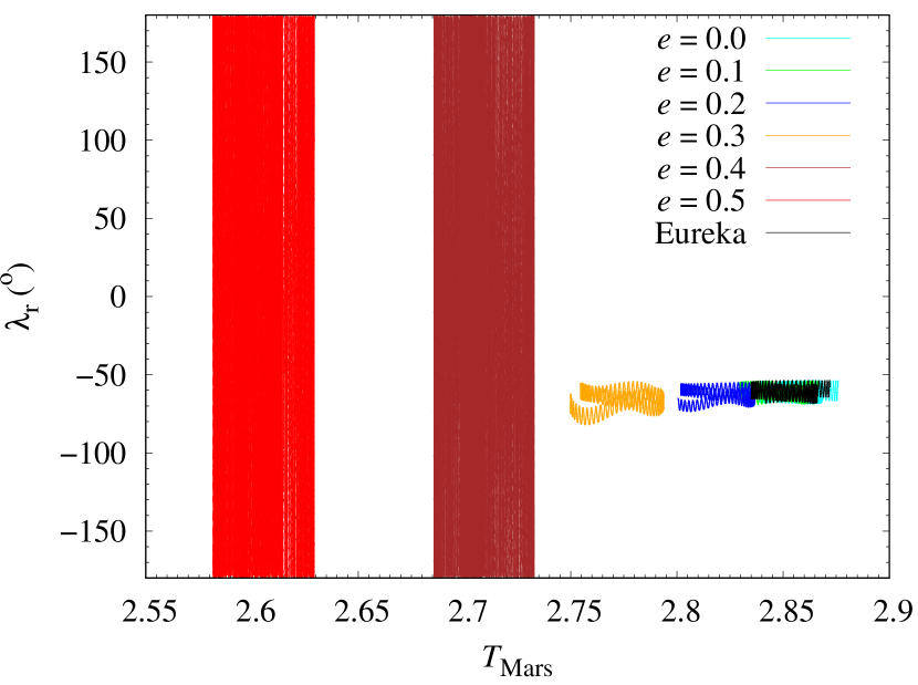
Figure 15: Effect of the eccentricity on the evolution of Eureka-like orbits. The nominal orbit of 5261 Eureka (1990 MB) and those of six other virtual test objects based on Eureka’s nominal orbit with $e=0.0$, 0.1, 0.2, 0.3, 0.4 and 0.5 have been integrated for 10⁵ yr forward in time. The evolution in the $T_{\rm Mars}$-$\lambda_{\rm r}$ plane is shown in the top panel. The bottom panel is a magnified version of the top one that focuses on Eureka and test orbits with $e=0.0$, 0.1, 0.2 and 0.3. The output time-step size is 1 yr.

The dynamical sampling displayed in Fig. 15 throws some light on the origin of the overall distribution of objects in Figs 1 and  5. New objects in the form of fragments may be formed with initially low values of the eccentricity that may increase secularly leading to smaller values of $T_{\rm Mars}$ or $T_{\rm Earth}$, transforming co-orbitals into passing objects whose position relative to the host planet is no longer controlled by the 1:1 mean-motion resonance. This evolutionary pathway appears particularly clear in the case of Mars co-orbitals (compare Figs 1 and  15); unfortunately, observational bias prevents a better assessment in the case of Earth co-orbitals (see Fig. 5) because the geometry of ground-based observations precludes the discovery of objects with mean longitudes different from that of Earth. It is however possible that unrelated objects or interlopers may also be present, creating pairs of objects, without any previous common dynamical history, whose values of the Tisserand parameter differ by very small amounts just by chance.

The median value of ${\Delta}T_{\rm Earth}$ is lower than that of ${\Delta}T_{\rm Mars}$, which suggest that fragmentations may be more frequent in Earth co-orbital space. However, when we consider the histograms of mean longitudes in Fig. 16, the sample of Earth co-orbitals appears to be biased in favour of those objects with mean longitudes close to that of Earth. This may however signal that fragmentations are mainly linked to quasi-satellites or asymmetric horseshoes or, more likely, to those objects that experience recurrent transitions between the quasi-satellite and horseshoe resonant states (perhaps because they are intrinsically more numerous). On the other hand, one object appears in both Table 4 and 5 and this is more consistent with cascades of disruptions than isolated events, a scenario favoured by Fatka et al. (2020). However, the most simple interpretation is that the data for the case of Earth may be strongly biased towards objects with low eccentricity and $\lambda_{\rm r}\sim 0{\degr}$ as these small bodies are physically the closest to the Earth and therefore more likely to be discovered.

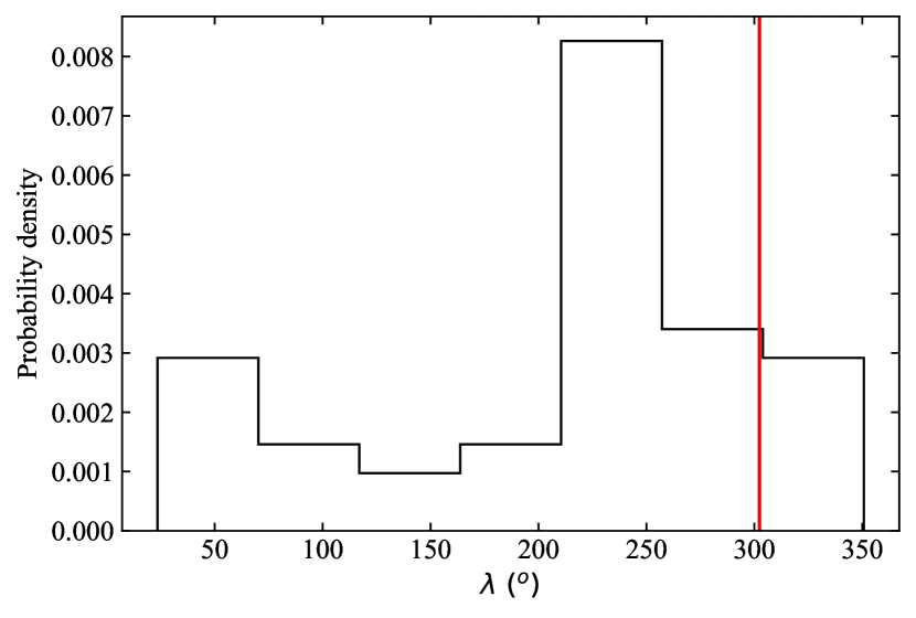
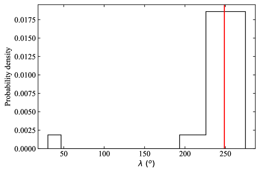
Figure 16: Distribution of mean longitudes for the samples of Mars co-orbitals (top panel) and Earth co-orbitals (bottom panel) discussed in this work. The mean longitudes of Mars and Earth are shown in red. The geometry of ground-based observations seems to make very difficult the discovery of objects with mean longitudes different from that of Earth.

Christou et al. (2020) argued that fragments produced during YORP-induced break-up events should be called YORPlets because the YORP mechanism produces them. Although 54509 YORP (2000 PH₅) itself, an irregular horseshoe to Earth that experiences the effects of the YORP mechanism, has been left out of our analysis because it has $e>0.2$, applying the same approach as before, we obtain Table 6 that includes 2015 JF₁₁ that has a very low ${\Delta}T_{\rm Earth}$ with respect to YORP.

Table 6: Similar to Table 4 but for YORP.

Object	$T_{\rm Earth}$	$\lambda_{\rm r}$ (°)	${\Delta}T_{\rm Earth}$
54509 YORP (2000 PH5)	2.945839220	$-$75.20226	–
2014 HL199	2.945164475	5.57231	0.000674745
2015 JF11	2.945883357	12.18048	0.000044137
2015 XX169	2.948366642	15.66149	0.002527422

One may contend that some objects mentioned above have poor orbit determinations: some data-arcs are as short as a few days. This is indeed true for many Earth co-orbitals that are dim and can only be sparsely observed. However and given the functional form of the Tisserand parameter in equation (1), even relatively poor orbit determinations may provide robust values of this parameter. The new co-orbitals identified in this research are further studied below.

6.1 New Mars co-orbitals

The three new Trojans follow tadpole orbits around Mars’ L₅; the candidate horseshoe librator follows a compound orbit that also encompasses Mars on one side (see Fig. 3, bottom panel). In addition to the Eureka family members, one additional L₅ Mars Trojan, 101429 (1998 VF₃₁), and one L₄, 121514 (1999 UJ₇) are known. Trojan 101429 was identified by Tabachnik & Evans (1999) and it is not as stable as those part of the Eureka family (see e.g. fig. 5 in de la Fuente Marcos & de la Fuente Marcos 2013a). In addition to having different orbital behaviour (Christou, 2013; de la Fuente Marcos & de la Fuente Marcos, 2013a), spectroscopic studies have confirmed that the physical nature of 101429 is different from that of most Eureka family members (Rivkin et al., 2007; Christou et al., 2021). The surface mineralogy of 121514 is also different (Borisov et al., 2019). The three new Mars Trojans identified in this work are mostly unstudied objects and the only data available about them are astrometric observations and their associated photometry. Small body 2020 VT₁ joins the subset of non-Trojan Mars co-orbitals discussed by Connors et al. (2005), although their objects move in more eccentric orbits. As a very recent discovery, it remains unstudied.

Table 7: Heliocentric Keplerian orbital elements of 2009 SE, 2018 EC₄, 2018 FC₄, and 2020 VT₁ used in this study. The orbit determination of 2009 SE is based on 56 observations spanning a data-arc of 3133 d or 8.58 yr (solution date, 2018-Apr-23 02:36:33 PDT), the one of 2018 EC₄ is based on 70 observations spanning a data-arc of 3131 d or 8.57 yr (solution date, 2020-May-30 05:28:03 PDT), and that of 2018 FC₄ is based on 35 observations spanning a data-arc of 790 d (solution date, 2020-Nov-11 09:52:11 PST). The orbit determination of 2020 VT₁is based on 28 observations spanning a data-arc of 24 d (solution date, 2020-Nov-15 04:55:38 PST). Values include the 1$\sigma$ uncertainty. The orbit determinations have been computed at epoch JD 2459000.5 that corresponds to 00:00:00.000 TDB on 2020 May 31 (J2000.0 ecliptic and equinox). Source: JPL’s SBDB.

Orbital parameter		2009 SE	2018 EC4	2018 FC4	2020 VT1
Semimajor axis, $a$ (au)	=	1.524472$\pm$0.000002	1.52357630$\pm$0.00000007	1.5238457$\pm$0.0000013	1.5231$\pm$0.0003
Eccentricity, $e$	=	0.0650794$\pm$0.0000010	0.06052671$\pm$0.00000012	0.017077$\pm$0.000006	0.16702$\pm$0.00010
Inclination, $i$ (°)	=	20.6248$\pm$0.0002	21.835796$\pm$0.000013	22.1437$\pm$0.0002	18.717$\pm$0.009
Longitude of the ascending node, $\Omega$ (°)	=	6.82030$\pm$0.00005	47.371564$\pm$0.000010	187.55390$\pm$0.00003	50.169$\pm$0.003
Argument of perihelion, $\omega$ (°)	=	354.156$\pm$0.010	344.1754$\pm$0.0004	52.009$\pm$0.007	296.191$\pm$0.012
Mean anomaly, $M$ (°)	=	240.916$\pm$0.012	203.4934$\pm$0.0005	4.660$\pm$0.007	315.410$\pm$0.013
Perihelion, $q$ (au)	=	1.425261$\pm$0.000002	1.43135923$\pm$0.00000015	1.497823$\pm$0.000009	1.26868$\pm$0.00013
Aphelion, $Q$ (au)	=	1.623684$\pm$0.000002	1.61579336$\pm$0.00000007	1.5498684$\pm$0.0000013	1.7774$\pm$0.0004
Absolute magnitude, $H$ (mag)	=	19.9$\pm$0.4	20.1$\pm$0.4	21.3$\pm$0.4	22.9$\pm$0.3

2009 SE. It was discovered on 2009 September 16 by the Catalina Sky Survey (CSS). Its orbit determination is robust as it is based on 56 observations spanning a data-arc of 3133 d or 8.58 yr (see Table 7). The size, shape and orientation of its orbit is similar to those of known L₅ Mars Trojans. It is a relatively bright object, suitable for future spectroscopic observations at an apparent visual magnitude of nearly 20. Its absolute magnitude is $H$=19.9 mag (assumed $G=0.15$), which suggests a diameter in the range $\sim$150–1200 m for an assumed albedo in the range 0.60–0.01. Masiero et al. (2018) have shown that albedos of $\sim$0.01 are possible but fairly rare; therefore, as asteroid size calculations are more sensitive to the lower bound than to the upper bound – because the albedo appears in the denominator – for a given range, smaller sizes are far more likely. Our calculations indicate that it is a stable L₅ Mars Trojan, see Fig. 17. From the nominal orbit (in black), its relative mean longitude oscillates around $-$60° with an amplitude of 70° and a libration period of 1430 yr, see Fig. 17, top panel. These values are comparable to those of 101429 and 121514 (see e.g. de la Fuente Marcos & de la Fuente Marcos 2013a). Figure 17, bottom panel, also shows the modulation with periodicity of about 200 000 yr pointed out originally by Mikkola et al. (1994) in the case of Eureka. Although its orbital evolution appears to be very stable on Myr time-scales (see Fig. 17, bottom panel), the libration amplitude is much larger than that of Eureka and this fact may make its long-term evolution less stable. Such results strongly suggest that 2009 SE, like 101429 and 121514, is not a member of the Eureka family, although a spectroscopic confirmation is still required. $N$-body simulations spanning Gyr time-scales show that both 101429 and 121514 may not be primordial Trojans but perhaps were captured about 4 Gyr ago (see e.g. de la Fuente Marcos & de la Fuente Marcos 2013a). Based on the analysis carried out here and what we already knew about the likely past orbital evolution of 101429 and 121514, we argue that 2009 SE may also be a captured object, not related to Eureka. This conclusion is robust when considering the relatively small uncertainties of the orbit determination in Table 7 (see Fig. 17, bottom panel, evolution of control orbits with Cartesian vectors separated from the nominal one).

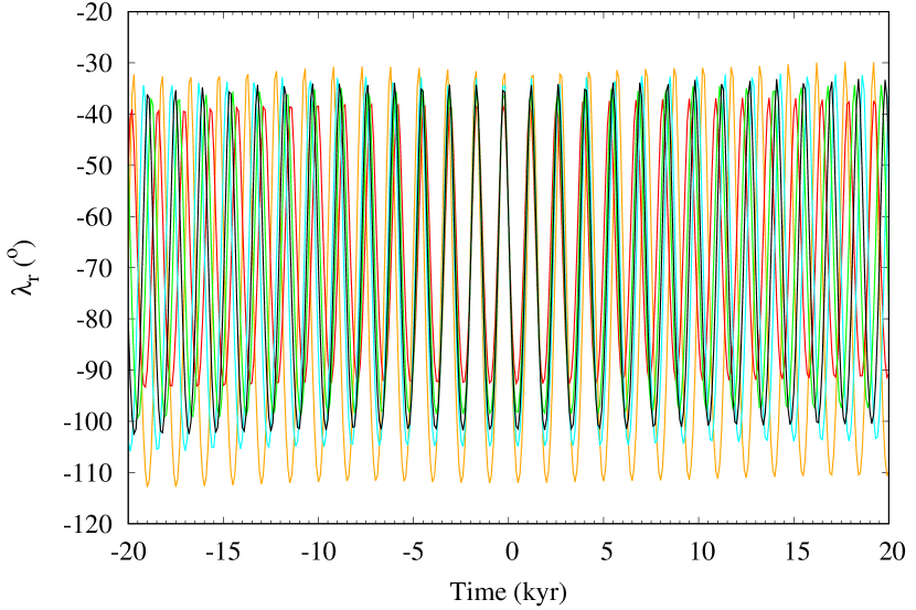
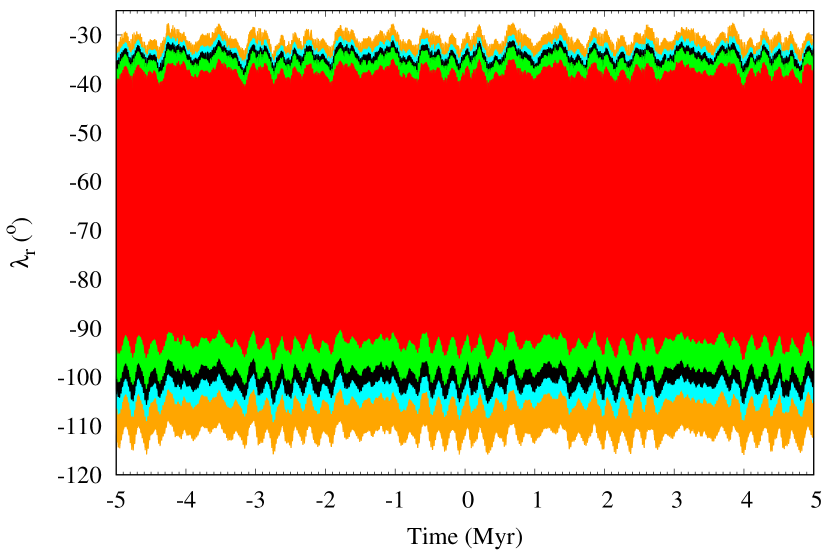
Figure 17: Evolution of the relative mean longitude with respect to Mars of 2009 SE. The time interval (-20, 20) kyr is shown in the top panel; the bottom panel displays the full calculations spanning 10 Myr. Our calculations include the nominal orbit (in black) as described by the orbit determination in Table 7 and those of control orbits or clones with Cartesian vectors separated $+$3$\sigma$ (in green), $-$3$\sigma$ (in cyan), $+$9$\sigma$ (in red), and $-$9$\sigma$ (in orange) from the nominal values in Table 9. The output time-step size is 100 yr.

2018 EC₄. Although this object was first observed on 2011 October 29 by the Pan-STARRS 1 telescope system at Haleakala, it remained unidentified until it was discovered by the Mt. Lemmon Survey (which is part of CSS) on 2018 March 10. As in the case of 2009 SE, its orbit determination is robust and based on 70 observations spanning a data-arc of 3131 d or 8.57 yr (see Table 7). Its orbit as well as apparent brightness and size are similar to those of 2009 SE. Our calculations also indicate that it is a stable L₅ Mars Trojan, see Fig. 18. The evolution of the nominal orbit (in black) shows that its relative mean longitude oscillates around $-$60° with an amplitude of 17° and a libration period of 1250 yr, see Fig. 18, top panel. These values are similar to those of 2011 SC₁₉₁ that may have been trapped at the Lagrangian L₅ point of Mars since the formation of the Solar system (see e.g. de la Fuente Marcos & de la Fuente Marcos 2013a). Ćuk et al. (2015) have argued that 2011 SC₁₉₁ may have been the first fragment ejected from Eureka. If distance from Eureka in the $T_{\rm Mars}$-$\lambda_{\rm r}$ plane (see Fig. 2) could be considered as an indication of the time passed since a given fragmentation event took place, then 2011 SC₁₉₁ is one of the most distant members of the Eureka family together with 2011 SP₁₈₉ and 2018 EC₄ (but see also Fig. 10) and they may have been produced first within the hierarchy of disintegrations induced by multiple YORP-induced spin-ups. That 2018 EC₄ is a probable member of the Eureka family is a robust conclusion when considering the small uncertainties of the orbit determination in Table 7 (see Fig. 18, bottom panel, evolution of control orbits with Cartesian vectors separated from the nominal one) although a spectroscopic confirmation is still required. Figure 18, bottom panel, also hints at the modulation with periodicity of about 200 000 yr pointed out originally by Mikkola et al. (1994) in the case of Eureka.

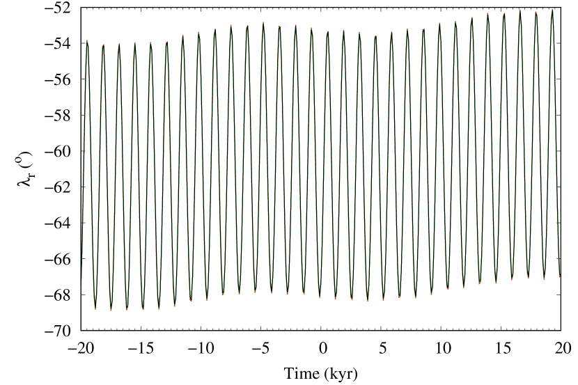
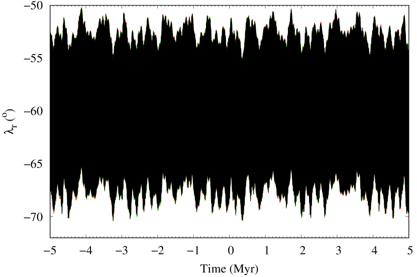
Figure 18: Same as Fig. 17 but for 2018 EC₄. In this case, even orbits separated $\pm$9$\sigma$ from the nominal one produce virtually identical evolution on Myr time-scales. Input values from Table 10.

2018 FC₄. This Mars Trojan and probable member of the Eureka family was also discovered by the Mt. Lemmon Survey that imaged it on 2018 March 21 although 2018 FC₄ also appeared in images acquired by the Pan-STARRS 1 telescope system the previous night. Its orbit determination is based on 35 observations spanning a data-arc of 790 d (see Table 7). Its absolute magnitude is $H$=21.3 mag (assumed $G=0.15$), which suggests a diameter in the range $\sim$100–800 m for an assumed albedo in the range 0.60–0.01 (as pointed out above, smaller sizes are far more likely). Figure 2 shows that 2018 FC₄ is perhaps the object closest to Eureka in the $T_{\rm Mars}$-$\lambda_{\rm r}$ plane. If future spectroscopic observations provide consistent results, 2018 FC₄ could be one of the youngest members of the Eureka family (otherwise, its low $T_{\rm Mars}$ relative to Eureka could be mere coincidence). Calculations similar to those performed in the cases of 2009 SE and 2018 EC₄ show that the orbital evolution of 2018 FC₄ is as stable as that of 2018 EC₄ (see Fig. 19) with the value of its relative mean longitude oscillating around $-$60° with an amplitude close to 20° and a libration period of nearly 1300 yr.

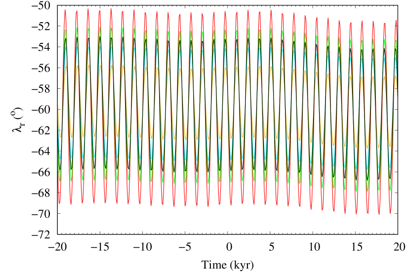
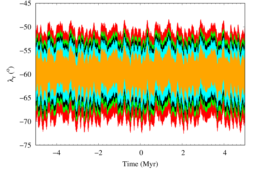
Figure 19: Same as Fig. 17 but for 2018 FC₄. As in the case of 2018 EC₄, even orbits separated $\pm$9$\sigma$ from the nominal one produce similar evolution on Myr time-scales. Input values from Table 11.

2020 VT₁. This Mars co-orbital candidate was discovered on 2020 November 10 by the Pan-STARRS 1 telescope system at Haleakala (Wainscoat et al., 2020), although it had been previously observed but not identified as a new discovery by the Mt. Lemmon Survey and Pan-STARRS 1 itself. Its orbit determination is based on 28 observations spanning a data-arc of 24 d and it is in need of improvement (see Table 7). Its absolute magnitude is $H$=22.9 mag (assumed $G=0.15$), which suggests a diameter in the range $\sim$40–300 m for an assumed albedo in the range 0.60–0.01 (as pointed out above, smaller sizes are far more likely). Calculations similar to those performed in the cases of 2009 SE, 2018 EC₄, and 2018 FC₄ indicate that the evolution of the nominal orbit of 2020 VT₁ is far less stable than those of the Trojans. Figure 3, bottom panel, shows that it could be a relatively recent capture and that it may follow an extended horseshoe path that encompasses Mars at the heel of one of the branches of the horseshoe. This object is the first of its kind to be found in Mars co-orbital space. A figure for the evolution of 2020 VT₁ has not been included here because the dispersion for orbits different from the nominal one is much larger than those displayed in Figs 17, 18 and 19.

6.2 New Earth co-orbitals

Our planet shares its orbit with a ring of captured asteroidal debris. The existence of the circumsolar Arjuna asteroid belt was first proposed by Rabinowitz et al. (1993) and further explored by e.g. Brasser & Wiegert (2008) and de la Fuente Marcos & de la Fuente Marcos (2013b), but its actual properties remain elusive. Most of its members are expected to be temporary co-orbitals of Earth: some of them could be relatively stable, long-term companions, but most are believed to be ephemeral and/or recurrent, short-term visitors that sometimes may become temporary satellites of our planet or minimoons. They tend to be small and dim, and they can only be detected and studied during flybys with Earth, which results in the strong observational bias pointed out above. This so-called Arjuna asteroid belt is a subset of the near-Earth asteroidal and cometary populations (near-Earth objects or NEOs) and includes captured interplanetary dust (Kortenkamp, 2013). The existence of orbital clusters in NEO space resulting from a combination of mean-motion resonances and catastrophic disruptions (rotation- or impact-induced) has been explored in the literature (see e.g. Fu et al. 2005; Schunová et al. 2012; de la Fuente Marcos & de la Fuente Marcos 2016b; Moskovitz et al. 2019; Jopek 2020) using the available but still limited observational evidence. The dynamics of objects part of the Arjuna asteroid belt is mostly controlled by Earth, but in some cases like that of 2020 CD₃ (Bolin et al., 2020; de la Fuente Marcos & de la Fuente Marcos, 2020; Fedorets et al., 2020), the Moon also plays a non-negligible role. Our analyses in Sections 4 and 5.2, have uncovered two new temporary Earth co-orbitals, not previously presented in the literature: 2020 PN₁ and 2020 PP₁. In addition, we have identified an object that was, until very recently (late November–early December), a quasi-satellite of our planet, 2020 XC.

2020 PN₁. This object was discovered on 2020 August 12 by the Asteroid Terrestrial-impact Last Alert System at Haleakala (Melnikov et al., 2020a). Its orbit determination (see Table 8) is robust and based on 41 observations spanning a data-arc of 361 d; it was rapidly improved because multiple precovery observations made by the Pan-STARRS 1 telescope system at Haleakala were found. Its absolute magnitude is $H$=25.5 mag (assumed $G=0.15$), which suggests a diameter in the range $\sim$10–100 m for an assumed albedo in the range 0.60–0.01 (as pointed out above, smaller sizes are far more likely). Figure 20, top panel, shows the evolution of the mean longitude difference of 2020 PN₁ for its nominal orbit determination and representative control orbits with Cartesian vectors separated $\pm$3$\sigma$ and $\pm$9$\sigma$ from the nominal values in Table 15. For integrations into the past, all the calculations indicate that it was a passing object that was only recently captured as a horseshoe librator to Earth. The evolution into the future predicts that it may continue in this co-orbital configuration and perhaps become a temporary quasi-satellite of our planet. In any case, predictions beyond about 500 yr may not be completely reliable. Horseshoes are thought to be the most numerous group among co-orbitals to Earth (see e.g. Wajer 2010; Christou & Asher 2011; de la Fuente Marcos & de la Fuente Marcos 2018b; Kaplan & Cengiz 2020).

2020 PP₁. This object was discovered on 2020 August 12 by the Pan-STARRS 1 telescope system at Haleakala (Melnikov et al., 2020b). Its orbit determination (see Table 8) is in need of improvement as it is based on 34 observations spanning a data-arc of 6 d. Its absolute magnitude is $H$=26.9 mag (assumed $G=0.15$), which suggests a diameter in the range $\sim$5–50 m for an assumed albedo in the range 0.60–0.01 (as pointed out above, smaller sizes are far more likely). Figure 20, bottom panel, displays the evolution of the mean longitude difference of 2020 PP₁ for its nominal orbit and those with Cartesian vectors separated $\pm$3$\sigma$ and $\pm$9$\sigma$ from the nominal values in Table 16. For integrations a few hundred years into the past or the future within $\pm$3$\sigma$ from the nominal orbit, predictions are consistent. It is currently leaving a quasi-satellite resonant state (but it is still engaged in it) to become a horseshoe librator. Its overall evolution exhibits a sequence of transitions between the quasi-satellite and horseshoe states. These recurrent transitions are similar to those found for Kamo‘oalewa (see Fig. 7, bottom panel) and several other known Earth co-orbitals (de la Fuente Marcos & de la Fuente Marcos, 2016a, c, 2018a). These episodes correspond to domain III evolution as described by Namouni (1999), i.e. horseshoe-retrograde satellite orbit transitions and librations.

Table 8: Heliocentric Keplerian orbital elements of 2020 PN₁, 2020 PP₁ and 2020 XC used in this study. The orbit determination of 2020 PN₁ is based on 41 observations spanning a data-arc of 361 d (solution date, 2020-Aug-28 09:16:12 PDT), the one of 2020 PP₁ is based on 34 observations spanning a data-arc of 6 d (solution date, 2020-Sep-11 07:48:43 PDT), and that of 2020 XC is based on 51 observations spanning a data-arc of 11 d (solution date, 2020-Dec-15 05:27:53 PST). Values include the 1$\sigma$ uncertainty. The orbit determinations have been computed at epoch JD 2459000.5 that corresponds to 00:00:00.000 TDB on 2020 May 31 (J2000.0 ecliptic and equinox). Source: JPL’s SBDB.

Orbital parameter		2020 PN1	2020 PP1	2020 XC
Semimajor axis, $a$ (au)	=	0.998105754$\pm$0.000000012	1.001715$\pm$0.000012	1.00170$\pm$0.00006
Eccentricity, $e$	=	0.1269557$\pm$0.0000009	0.07384$\pm$0.00007	0.10738$\pm$0.00002
Inclination, $i$ (°)	=	4.80807$\pm$0.00003	5.827$\pm$0.007	0.760$\pm$0.002
Longitude of the ascending node, $\Omega$ (°)	=	145.63610$\pm$0.00002	141.0248$\pm$0.0004	71.751$\pm$0.006
Argument of perihelion, $\omega$ (°)	=	55.40365$\pm$0.00002	44.14$\pm$0.03	269.31$\pm$0.03
Mean anomaly, $M$ (°)	=	32.06964$\pm$0.00011	56.64$\pm$0.03	254.83$\pm$0.02
Perihelion, $q$ (au)	=	0.8713906$\pm$0.0000009	0.92775$\pm$0.00006	0.89413$\pm$0.00007
Aphelion, $Q$ (au)	=	1.124820928$\pm$0.000000013	1.075679$\pm$0.000013	1.10926$\pm$0.00006
Absolute magnitude, $H$ (mag)	=	25.5$\pm$0.4	26.9$\pm$0.4	29.0$\pm$0.4

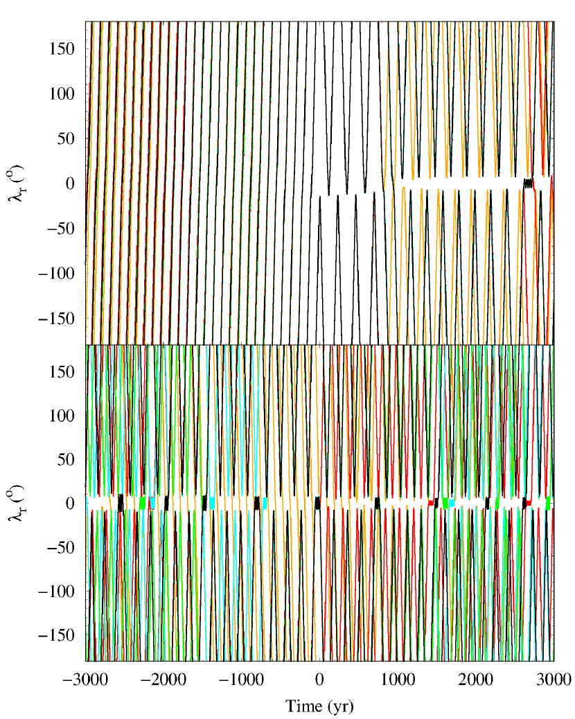
Figure 20: Evolution of the mean longitude difference of 2020 PN₁ (top panel) and 2020 PP₁ (bottom panel) and Earth. Our calculations include the nominal orbits (in black) as described by the orbit determinations in Table 8 and those of representative control orbits or clones with Cartesian vectors separated $+$3$\sigma$ (in green), $-$3$\sigma$ (in cyan), $+$9$\sigma$ (in red), and $-$9$\sigma$ (in orange) from the nominal values in Tables 15 and 16. The origin of time is epoch 2459000.5 TDB.

2020 XC. This object was discovered by the Mt. Lemmon Survey on 2020 December 4 (Rankin et al., 2020). Its orbit determination (see Table 8) is also in need of improvement as it is based on 51 observations spanning a data-arc of 11 d. Its absolute magnitude is $H$=29.0 mag (assumed $G=0.15$) and it is probably a secondary fragment of a larger object. It experienced a close encounter with the Earth on 2020 November 30 at 0.0008 au that altered its co-orbital status dramatically. Figure 21 shows that prior to this encounter, 2020 XC was a quasi-satellite of our planet, but after the flyby it became a passing body. Therefore, it is no longer co-orbital to Earth, but it has been included here because it was one of them at the standard epoch used in this study, 2459000.5 TDB.

Figure 21: Evolution of the mean longitude difference of 2020 XC and Earth. The output time-step size is 0.01 yr, the origin of time is epoch 2459000.5 TDB, and only the nominal orbit (see Table 8) has been displayed.

7 Conclusions

In this paper, we have applied a novel approach to estimate the importance of rotation-induced YORP break-up events in Earth co-orbital space using data from Mars co-orbitals. Within the framework of the Tisserand’s criterion (Tisserand, 1896), we assumed that two co-orbital (to a certain planet) minor bodies resulting from a YORP break-up event should have approximately the same values of the Tisserand parameter. The hypothesis is validated using data of Mars co-orbitals with eccentricity below 0.2 and machine-learning techniques. The approach is subsequently applied to an equivalent group of Earth co-orbitals. The main conclusions of our study are:

1. We identify three new L₅ Mars Trojans: 2009 SE, 2018 EC₄ and 2018 FC₄. Two of them, 2018 EC₄ and 2018 FC₄, are very probably linked to 5261 Eureka (1990 MB). We argue that 2009 SE may be a captured object, not related to Eureka.

2. We confirm in the $T_{\rm Mars}$-$\lambda_{\rm r}$ plane the very strong asymmetry between the L₄ and L₅ Trojan clouds of Mars.

3. We identify one new Mars co-orbital candidate, 2020 VT₁, that may follow an extended horseshoe path that encompasses Mars at the heel of one of the branches. This object is the first of its kind to be found in Mars co-orbital space.

4. We identify two new Earth co-orbitals: 2020 PN₁, that follows a horseshoe path, and 2020 PP₁, a quasi-satellite.

5. We identify a former quasi-satellite to Earth, 2020 XC, that was very recently ejected from co-orbital space after a close flyby.

6. We identify clustering in the $T_{\rm Earth}$-$\lambda_{\rm r}$ plane that could be compatible with the outcome of recent YORP break-up events. The cluster with most members is probably associated with 469219 Kamo‘oalewa (2016 HO₃); 2020 PP₁ follows an orbital evolution that closely resembles that of Kamo‘oalewa.

7. Clustering algorithms and numerical simulations both suggest that 2020 KZ₂ and Kamo‘oalewa could be related.

The existence, for both Earth and Mars, of recently captured co-orbitals experiencing similar orbital evolution is confirmed with the identification of 2020 PN₁ (see Fig. 20, top panel) and 2020 VT₁ (see Fig. 3, bottom panel). Although most known Mars co-orbitals are long-term stable and all known Earth co-orbitals are not, the presence of 2020 VT₁ suggests that, much like Earth, Mars may host a sizeable population of transient co-orbitals.

Although the thermal YORP mechanism may have spun up Eureka, leading to the formation of the Eureka family, Mars Trojans may also be the results of impacts (Polishook et al., 2017). A giant impact (Marinova, Aharonson & Asphaug, 2008; Hyodo & Genda, 2018) may have led to the formation of the Martian moons Phobos and Deimos as well (Citron, Genda & Ida, 2015; Hyodo et al., 2017a, b, 2018; Hansen, 2018; Pignatale et al., 2018). Separate origins for the known Mars Trojans have previously been suggested by Rivkin et al. (2007) and Trilling et al. (2007), but see also the discussion in Christou et al. (2021). Our conclusions for the Mars Trojans are however independent of the actual origin of the objects (YORP-induced break-up, impact debris from Mars or collisions between asteroids) as they focus on dynamical evolution and clustering in the $T_{\rm Mars}$-$\lambda_{\rm r}$ plane. A similar statement can be made regarding our conclusions for the Earth co-orbitals that may come from rotational fission events, Lunar impacts or catastrophic NEO collisions (among other sources).

The analysis of the structure in the $T_{\rm P}$-$\lambda_{\rm r}$ plane by itself cannot confirm genetic associations between planetary co-orbitals, but it can be used to select candidates worthy of further study (numerical and spectroscopic). In this context, the study of the $T_{\rm P}$-$\lambda_{\rm r}$ plane provides evidence akin to that coming from orbital similarity criteria (see e.g. Drummond 1991, 2000; Jopek 1993; Kholshevnikov et al. 2016). It can be argued that the use of $T_{\rm P}$ as an orbital similarity criterion has strong limitations that may be absent from other widely used orbital similarity criteria. Figure 15 shows that the value of $T_{\rm Mars}$ for Eureka changes by about 0.02 in 10⁵ yr; therefore, small values of ${\Delta}T_{\rm Mars}$ cannot be used to argue for a genetic relationship. This argument is robust in the case of the present-day Mars Trojans if they have remained in their present orbits for time-scales of the order of the age of the Solar system as two initially almost identical $T_{\rm Mars}$ corresponding to two fragments may have had time to randomize parameters sufficiently within the quasi-invariant boundaries (see Fig. 15). This view gains further support if the objects under consideration have very different values of $\lambda_{\rm r}$ and they experience relatively close approaches at high relative speeds. Under these conditions, the existence of small values of ${\Delta}T_{\rm Mars}$ can be attributed to mere coincidence and most if not all pairings could be spurious, placing some of the conclusions of our study in doubt. This line of reasoning however loses most of its credence when considering dynamically young objects like known Earth co-orbitals that may also experience relatively close encounters with both Earth and the Moon. In this case, small values of ${\Delta}T_{\rm Earth}$ can certainly be used to argue for a genetic relationship, unless the size of the population is very large so sampling small values of ${\Delta}T_{\rm Earth}$ is far more probable.

Although we have to admit that the simplest hypothesis regarding the existence of small values of ${\Delta}T_{\rm Earth}$ is that they could be all linked to random orbital alignments, it is possible to design a numerical experiment to confirm or reject the feasibility of scenarios other than mere coincidence for these dynamically young objects. As a test of the implications that a genetic relationship may have on ${\Delta}T_{\rm Earth}$ for Earth co-orbitals, we have performed a numerical experiment with the nominal orbit of Kamo‘oalewa and two control orbits with Cartesian vectors separated $+$9000$\sigma$ and $-$9000$\sigma$ in terms of velocity from the nominal values in Table 12 to study the evolution of $a$, $e$, $i$ and $T_{\rm Earth}$ (i.e. the initial positions are the same, but the starting velocities are different). This experiment is equivalent to assuming that two fragments of Kamo‘oalewa left its surface with relative velocities close to 100 m s^-1. Figure 22 shows the results of this experiment: the maximum relative variation in $T_{\rm Earth}$ is about 0.3 per cent while the equivalent results for $e$ and $i$ are 57 per cent and 75 per cent, respectively. For genetically related fragments, the value of ${\Delta}T_{\rm Earth}$ may remain well under 0.014 even after 10⁴ yr while the orbits could become rather different in terms of inclination and eccentricity after just 10³ yr. In other words, Fig. 22 shows that the value of ${\Delta}T_{\rm Earth}$ can remain as small as the values reported in Tables 4 and 5 for a significant amount of time although the shape and space orientation of the orbit of the fragment drifted noticeably away from those of the parent body.

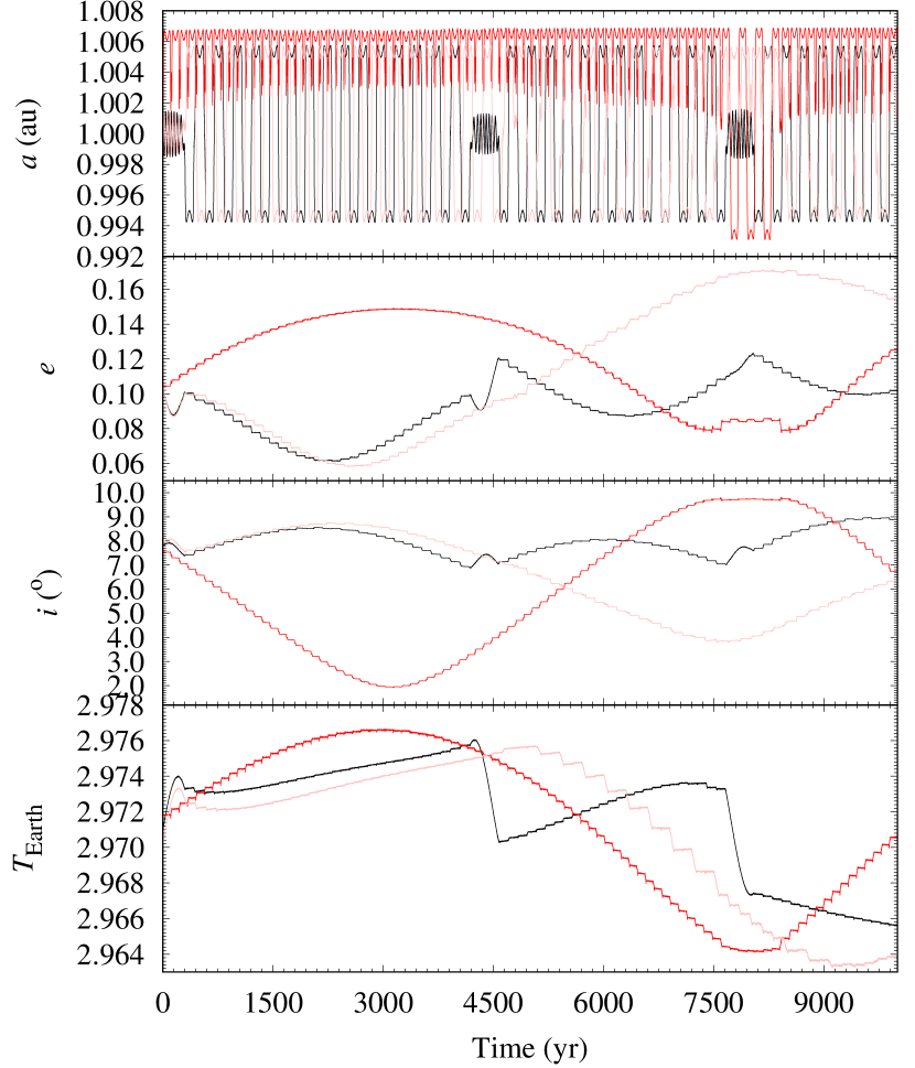
Figure 22: Evolution of the semimajor axis, $a$ (top panel), of the nominal orbit (in black) of 469219 Kamo‘oalewa (2016 HO₃) as described by the orbit determination in Table 3 and those of control orbits or clones with Cartesian vectors separated $+$9000$\sigma$ (in red) and $-$9000$\sigma$ (in pink) in terms of velocity from the nominal values in Table 12, i.e. the initial positions are the same, but the starting velocities are different. The second to top panel shows the evolution of the eccentricity, $e$, for the same sample of control orbits. The second to bottom panel displays the inclination, $i$. The bottom panel shows the variation of the Tisserand’s parameter, $T_{\rm Earth}$. The origin of time is epoch 2459000.5 TDB.

It has sometimes been argued that planetary co-orbitals are the result of capture events or a side effect of planet formation itself (i.e. the Jovian Trojans), our analysis within the context of the Trojans of Mars provides support to a new paradigm where production of co-orbitals may have more than two active channels. This is particularly interesting in the region of the terrestrial planets where both catastrophic and binary disruptions, and production of debris via planetary impacts, could be possible.

Data Availability

The data underlying this paper were accessed from JPL’s SBDB (https://ssd.jpl.nasa.gov/sbdb.cgi). The derived data generated in this research will be shared on reasonable request to the corresponding author.

Appendix A Input data

Here, we include the barycentric Cartesian state vectors of the various objects mentioned in the main text of this paper. These vectors and their uncertainties have been used to perform the calculations discussed above and generate those figures that display the time evolution of orbital parameters and the histograms of the close encounters of pairs of objects. For example: a new value of the $X$-component of the state vector is computed as $X_{\rm c}=X+\sigma_{X}\ r$, where $r$ is an univariate Gaussian random number, and $X$ and $\sigma_{X}$ are the mean value and its 1$\sigma$ uncertainty in the corresponding table.

Table 9: Barycentric Cartesian state vector of 2009 SE: components and associated 1$\sigma$ uncertainties. Epoch as in Table 7. Source: JPL’s SBDB.

Component		value$\pm$1$\sigma$ uncertainty
$X$ (au)	=	$-$9.044249670510914$\times 10^{-1}$$\pm$3.95127734$\times 10^{-5}$
$Y$ (au)	=	$-$1.219519611628439$\times 10^{+0}$$\pm$4.43547485$\times 10^{-6}$
$Z$ (au)	=	$-$4.181102558282555$\times 10^{-1}$$\pm$2.03602531$\times 10^{-6}$
$V_{X}$ (au d-1)	=	1.143843538936524$\times 10^{-2}$$\pm$3.40882338$\times 10^{-7}$
$V_{Y}$ (au d-1)	=	$-$6.448195605210014$\times 10^{-3}$$\pm$2.27814124$\times 10^{-7}$
$V_{Z}$ (au d-1)	=	$-$2.919772593230286$\times 10^{-3}$$\pm$9.01993401$\times 10^{-8}$

Table 10: Barycentric Cartesian state vector of 2018 EC₄: components and associated 1$\sigma$ uncertainties. Epoch as in Table 7. Source: JPL’s SBDB.

Component		value$\pm$1$\sigma$ uncertainty
$X$ (au)	=	$-$9.930212176028788$\times 10^{-1}$$\pm$4.53081481$\times 10^{-7}$
$Y$ (au)	=	$-$1.261773631639331$\times 10^{+0}$$\pm$2.66927453$\times 10^{-7}$
$Z$ (au)	=	$-$5.298080705059578$\times 10^{-2}$$\pm$1.55233589$\times 10^{-7}$
$V_{X}$ (au d-1)	=	9.928799979516468$\times 10^{-3}$$\pm$6.94939332$\times 10^{-9}$
$V_{Y}$ (au d-1)	=	$-$7.155133944288653$\times 10^{-3}$$\pm$4.37147830$\times 10^{-9}$
$V_{Z}$ (au d-1)	=	$-$4.870041988110999$\times 10^{-3}$$\pm$3.33948347$\times 10^{-9}$

Table 11: Barycentric Cartesian state vector of 2018 FC₄: components and associated 1$\sigma$ uncertainties. Epoch as in Table 7. Source: JPL’s SBDB.

Component		value$\pm$1$\sigma$ uncertainty
$X$ (au)	=	$-$6.647626395087657$\times 10^{-1}$$\pm$5.55753437$\times 10^{-6}$
$Y$ (au)	=	$-$1.251996334582715$\times 10^{+0}$$\pm$4.96594761$\times 10^{-6}$
$Z$ (au)	=	4.726742793843942$\times 10^{-1}$$\pm$7.04561654$\times 10^{-6}$
$V_{X}$ (au d-1)	=	1.268921413237325$\times 10^{-2}$$\pm$9.38769625$\times 10^{-8}$
$V_{Y}$ (au d-1)	=	$-$5.581094365762196$\times 10^{-3}$$\pm$2.49673168$\times 10^{-8}$
$V_{Z}$ (au d-1)	=	2.929559280832830$\times 10^{-3}$$\pm$1.95051109$\times 10^{-8}$

Table 12: Barycentric Cartesian state vector of 469219 Kamo‘oalewa (2016 HO₃): components and associated 1$\sigma$ uncertainties. Epoch as in Table 3. Source: JPL’s SBDB.

Component		value$\pm$1$\sigma$ uncertainty
$X$ (au)	=	$-$5.449319912718597$\times 10^{-1}$$\pm$4.16666980$\times 10^{-7}$
$Y$ (au)	=	$-$9.113174005478253$\times 10^{-1}$$\pm$6.84410519$\times 10^{-8}$
$Z$ (au)	=	1.681543176484481$\times 10^{-2}$$\pm$6.13612239$\times 10^{-8}$
$V_{X}$ (au d-1)	=	1.436478550115864$\times 10^{-2}$$\pm$4.18885560$\times 10^{-9}$
$V_{Y}$ (au d-1)	=	$-$6.974713611012369$\times 10^{-3}$$\pm$1.47221869$\times 10^{-9}$
$V_{Z}$ (au d-1)	=	$-$2.182420313697609$\times 10^{-3}$$\pm$4.40382271$\times 10^{-9}$

Table 13: Barycentric Cartesian state vector of 2016 FU₁₂: components and associated 1$\sigma$ uncertainties. Epoch as in Table 3. Source: JPL’s SBDB.

Component		value$\pm$1$\sigma$ uncertainty
$X$ (au)	=	$-$7.349994733814580$\times 10^{-1}$$\pm$8.90684866$\times 10^{-3}$
$Y$ (au)	=	$-$9.037930038260460$\times 10^{-1}$$\pm$5.26547287$\times 10^{-3}$
$Z$ (au)	=	5.409610013000898$\times 10^{-3}$$\pm$4.90283157$\times 10^{-4}$
$V_{X}$ (au d-1)	=	1.100523434296072$\times 10^{-2}$$\pm$1.18547355$\times 10^{-4}$
$V_{Y}$ (au d-1)	=	$-$9.543786932245953$\times 10^{-3}$$\pm$1.06494665$\times 10^{-4}$
$V_{Z}$ (au d-1)	=	5.372770530624185$\times 10^{-4}$$\pm$5.47519985$\times 10^{-6}$

Table 14: Barycentric Cartesian state vector of 2020 KZ₂: components and associated 1$\sigma$ uncertainties. Epoch as in Table 3. Source: JPL’s SBDB.

Component		value$\pm$1$\sigma$ uncertainty
$X$ (au)	=	$-$3.773666435827534$\times 10^{-1}$$\pm$3.18219205$\times 10^{-5}$
$Y$ (au)	=	$-$9.577429216614861$\times 10^{-1}$$\pm$2.04064633$\times 10^{-5}$
$Z$ (au)	=	$-$8.960329684632281$\times 10^{-3}$$\pm$1.34705032$\times 10^{-5}$
$V_{X}$ (au d-1)	=	1.541735728765344$\times 10^{-2}$$\pm$7.11067379$\times 10^{-7}$
$V_{Y}$ (au d-1)	=	$-$5.969582318369662$\times 10^{-3}$$\pm$5.08277865$\times 10^{-8}$
$V_{Z}$ (au d-1)	=	$-$2.093381081617893$\times 10^{-3}$$\pm$3.11097775$\times 10^{-6}$

Table 15: Barycentric Cartesian state vector of 2020 PN₁: components and associated 1$\sigma$ uncertainties. Epoch as in Table 8. Source: JPL’s SBDB.

Component		value$\pm$1$\sigma$ uncertainty
$X$ (au)	=	$-$4.241165537792646$\times 10^{-1}$$\pm$4.10976065$\times 10^{-7}$
$Y$ (au)	=	$-$7.815068992626035$\times 10^{-1}$$\pm$1.25238788$\times 10^{-6}$
$Z$ (au)	=	7.470552943322972$\times 10^{-2}$$\pm$4.26388149$\times 10^{-7}$
$V_{X}$ (au d-1)	=	1.610713932302730$\times 10^{-2}$$\pm$8.18961953$\times 10^{-10}$
$V_{Y}$ (au d-1)	=	$-$1.021489969786571$\times 10^{-2}$$\pm$3.28094580$\times 10^{-8}$
$V_{Z}$ (au d-1)	=	$-$5.587679529869726$\times 10^{-5}$$\pm$1.55793533$\times 10^{-9}$

Table 16: Barycentric Cartesian state vector of 2020 PP₁: components and associated 1$\sigma$ uncertainties. Epoch as in Table 8. Source: JPL’s SBDB.

Component		value$\pm$1$\sigma$ uncertainty
$X$ (au)	=	$-$3.443442683083884$\times 10^{-1}$$\pm$1.82961900$\times 10^{-5}$
$Y$ (au)	=	$-$8.916362488037327$\times 10^{-1}$$\pm$5.85976394$\times 10^{-5}$
$Z$ (au)	=	9.314163806080564$\times 10^{-2}$$\pm$1.00891106$\times 10^{-4}$
$V_{X}$ (au d-1)	=	1.620597866455574$\times 10^{-2}$$\pm$3.80871529$\times 10^{-7}$
$V_{Y}$ (au d-1)	=	$-$7.401387669318608$\times 10^{-3}$$\pm$1.46198049$\times 10^{-6}$
$V_{Z}$ (au d-1)	=	$-$4.536468695716349$\times 10^{-4}$$\pm$4.45907592$\times 10^{-7}$

References

- Aarseth (2003) Aarseth S. J., 2003, Gravitational N-body Simulations. Cambridge Univ. Press, Cambridge, p. 27
- Arthur & Vassilvitskii (2007) Arthur D., Vassilvitskii S., 2007, in Gabow H., ed., Proceedings of the eighteenth annual ACM-SIAM symposium on discrete algorithms, Society for Industrial and Applied Mathematics Philadelphia, PA, USA, p. 1027
- Benitez & Gallardo (2008) Benitez F., Gallardo T., 2008, Celest. Mech. Dyn. Astron., 101, 289
- Bodewits et al. (2011) Bodewits D., Kelley M. S., Li J.-Y., Landsman W. B., Besse S., A’Hearn M. F., 2011, ApJ, 733, L3
- Bolin et al. (2020) Bolin B. T. et al., 2020, ApJ, 900, L45
- Borisov et al. (2017) Borisov G., Christou A., Bagnulo S., Cellino A., Kwiatkowski T., Dell’Oro A., 2017, MNRAS, 466, 489
- Borisov et al. (2018) Borisov G., Christou A. A., Colas F., Bagnulo S., Cellino A., Dell’Oro A., 2018, A&A, 618, A178
- Borisov et al. (2019) Borisov G., Christou A., Bagnulo S., Cellino A., Dell’Oro A., 2019, EPSC-DPS Joint Meeting 2019, 13, EPSC-DPS2019-1254
- Bottke et al. (2006) Bottke W. F., Vokrouhlický D., Rubincam D. P., Nesvorný D., 2006, Annu. Rev. Earth Planet. Sci., 34, 157
- Brasser & Wiegert (2008) Brasser R., Wiegert P., 2008, MNRAS, 386, 2031
- Bressi et al. (2008) Bressi T. H. et al., 2008, MPEC Circ., MPEC 2008-D12
- Buitinck et al. (2013) Buitinck L. et al., 2013, in Blockeel H., Kersting K., Nijssen S., Zelezny F., eds, ECML PKDD Workshop: Languages for Data Mining and Machine Learning, Springer-Verlag Berlin Heidelberg, p. 108
- Carruba, Aljbaae & Lucchini (2019) Carruba V., Aljbaae S., Lucchini A., 2019, MNRAS, 488, 1377
- Carruba, Ramos & Spoto (2020) Carruba V., Ramos L. G. M., Spoto F., 2020, MNRAS, 493, 2556
- Carruba et al. (2020a) Carruba V., Spoto F., Barletta W., Aljbaae S., Fazenda Á. L., Martins B., 2020a, Nature Astronomy, 4, 83
- Carruba et al. (2020b) Carruba V., Aljbaae S., Domingos R. C., Lucchini A., Furlaneto P., 2020b, MNRAS, 496, 540
- Christou (2013) Christou A. A., 2013, Icarus, 224, 144
- Christou & Murray (1999) Christou A. A., Murray C. D., 1999, MNRAS, 303, 806
- Christou & Asher (2011) Christou A. A., Asher D. J., 2011, MNRAS, 414, 2965
- Christou et al. (2017) Christou A. A., Borisov G., Dell’Oro A., Cellino A., Bagnulo S., 2017, Icarus, 293, 243
- Christou et al. (2020) Christou A. A., Borisov G., Dell’Oro A., Jacobson S. A., Cellino A., Unda-Sanzana E., 2020, Icarus, 335, 113370
- Christou et al. (2021) Christou A. A., Borisov G., Dell’Oro A., Cellino A., Devogèle M., 2021, Icarus, 354, 113994
- Citron, Genda & Ida (2015) Citron R. I., Genda H., Ida S., 2015, Icarus, 252, 334
- Connors, Wiegert & Veillet (2011) Connors M., Wiegert P., Veillet C., 2011, Nature, 475, 481
- Connors et al. (2005) Connors M., Stacey G., Brasser R., Wiegert P., 2005, Planet. Space Sci., 53, 617
- Ćuk, Christou & Hamilton (2015) Ćuk M., Christou A. A., Hamilton D. P., 2015, Icarus, 252, 339
- de la Fuente Marcos & de la Fuente Marcos (2012) de la Fuente Marcos C., de la Fuente Marcos R., 2012, MNRAS, 427, 728
- de la Fuente Marcos & de la Fuente Marcos (2013a) de la Fuente Marcos C., de la Fuente Marcos R., 2013a, MNRAS, 432, L31
- de la Fuente Marcos & de la Fuente Marcos (2013b) de la Fuente Marcos C., de la Fuente Marcos R., 2013b, MNRAS, 434, L1
- de la Fuente Marcos & de la Fuente Marcos (2016a) de la Fuente Marcos C., de la Fuente Marcos R., 2016a, Ap&SS, 361, 16
- de la Fuente Marcos & de la Fuente Marcos (2016b) de la Fuente Marcos C., de la Fuente Marcos R., 2016b, MNRAS, 456, 2946
- de la Fuente Marcos & de la Fuente Marcos (2016c) de la Fuente Marcos C., de la Fuente Marcos R., 2016c, MNRAS, 462, 3441
- de la Fuente Marcos & de la Fuente Marcos (2018a) de la Fuente Marcos C., de la Fuente Marcos R., 2018a, MNRAS, 473, 3434
- de la Fuente Marcos & de la Fuente Marcos (2018b) de la Fuente Marcos C., de la Fuente Marcos R., 2018b, MNRAS, 473, 2939
- de la Fuente Marcos & de la Fuente Marcos (2019) de la Fuente Marcos C., de la Fuente Marcos R., 2019, MNRAS, 483, L37
- de la Fuente Marcos & de la Fuente Marcos (2020) de la Fuente Marcos C., de la Fuente Marcos R., 2020, MNRAS, 494, 1089
- Dmitriev, Lupovka & Gritsevich (2015) Dmitriev V., Lupovka V., Gritsevich M., 2015, Planet. Space Sci., 117, 223
- Drummond (1991) Drummond J. D., 1991, Icarus, 89, 14
- Drummond (2000) Drummond J. D., 2000, Icarus, 146, 453
- Dvorak, Lhotka & Zhou (2012) Dvorak R., Lhotka C., Zhou L., 2012, A&A, 541, A127
- Farinella & Davis (1992) Farinella P., Davis D. R., 1992, Icarus, 97, 111
- Fatka, Pravec & Vokrouhlický (2020) Fatka P., Pravec P., Vokrouhlický D., 2020, Icarus, 338, 113554
- Fedorets et al. (2020) Fedorets G. et al., 2020, AJ, 160, 277
- Freedman & Diaconis (1981) Freedman D., Diaconis P., 1981, Z. Wahrscheinlichkeitstheorie verw. Gebiete, 57, 453
- Fu et al. (2005) Fu H., Jedicke R., Durda D. D., Fevig R., Scotti J. V., 2005, Icarus, 178, 434
- Ginsburg et al. (2019) Ginsburg A. et al., 2019, AJ, 157, 98
- Giorgini (2011) Giorgini J., 2011, in Capitaine N., ed., Proceedings of the Journées 2010 “Systèmes de référence spatio-temporels” (JSR2010): New challenges for reference systems and numerical standards in astronomy, Observatoire de Paris, Paris, p. 87
- Giorgini (2015) Giorgini J. D., 2015, IAU General Assembly, Meeting #29, 22, 2256293
- Hainaut et al. (2019) Hainaut O. R. et al., 2019, A&A, 628, A48
- Hansen (2018) Hansen B. M. S., 2018, MNRAS, 475, 2452
- Hunter (2007) Hunter J. D., 2007, CSE, 9, 90
- Hyodo & Genda (2018) Hyodo R., Genda H., 2018, ApJ, 856, L36
- Hyodo et al. (2017a) Hyodo R., Genda H., Charnoz S., Rosenblatt P., 2017a, ApJ, 845, 125
- Hyodo et al. (2017b) Hyodo R., Rosenblatt P., Genda H., Charnoz S., 2017b, ApJ, 851, 122
- Hyodo et al. (2018) Hyodo R., Genda H., Charnoz S., Pignatale F. C. F., Rosenblatt P., 2018, ApJ, 860, 150
- Jacobson & Scheeres (2011) Jacobson S. A., Scheeres D. J., 2011, Icarus, 214, 161
- Jopek (1993) Jopek T. J., 1993, Icarus, 106, 603
- Jopek (2020) Jopek T. J., 2020, MNRAS, 494, 680
- Jutzi et al. (2010) Jutzi M., Michel P., Benz W., Richardson D. C., 2010, Icarus, 207, 54
- Kaplan & Cengiz (2020) Kaplan M., Cengiz S., 2020, MNRAS, 496, 4420
- Kelso (2009) Kelso T. S., 2009, in Ryan S., ed., Proceedings of the Advanced Maui Optical and Space Surveillance Technologies Conference, The Maui Economic Development Board., E3
- Kholshevnikov et al. (2016) Kholshevnikov K. V., Kokhirova G. I., Babadzhanov P. B., Khamroev U. H., 2016, MNRAS, 462, 2275
- Kortenkamp (2013) Kortenkamp S. J., 2013, Icarus, 226, 1550
- Kwiatkowski et al. (2009) Kwiatkowski T. et al., 2009, A&A, 495, 967
- Lloyd (1982) Lloyd S. P., 1957, IEEE Transactions on Information Theory, 28, 129
- MacQueen (1967) MacQueen J. B., 1967, in Le Cam L. M., Neyman, J., eds, Proceedings of 5th Berkeley Symposium on Mathematical Statistics and Probability, Volume 1: Statistics, University of California Press, p. 281
- Makino (1991) Makino J., 1991, ApJ, 369, 200
- Marinova, Aharonson & Asphaug (2008) Marinova M. M., Aharonson O., Asphaug E., 2008, Nature, 453, 1216
- Marzari et al. (2020) Marzari F., Rossi A., Golubov O., Scheeres D. J., 2020, AJ, 160, 128
- Masiero et al. (2013) Masiero J. R., Mainzer A. K., Bauer J. M., Grav T., Nugent C. R., Stevenson R., 2013, ApJ, 770, 7
- Masiero et al. (2018) Masiero J. R. et al., 2018, AJ, 156, 60
- McIntyre (2019) McIntyre K. J., 2019, MA thesis, The University of North Dakota
- Melnikov et al. (2020a) Melnikov S. et al., 2020a, MPEC Circ., MPEC 2020-P66
- Melnikov et al. (2020b) Melnikov S. et al., 2020b, MPEC Circ., MPEC 2020-P68
- Mikkola & Innanen (1994) Mikkola S., Innanen K., 1994, AJ, 107, 1879
- Mikkola et al. (1994) Mikkola S., Innanen K., Muinonen K., Bowell E., 1994, Celest. Mech. Dyn. Astron., 58, 53
- Mikkola et al. (2006) Mikkola S., Innanen K., Wiegert P., Connors M., Brasser R., 2006, MNRAS, 369, 15
- Morais & Morbidelli (2002) Morais M. H. M., Morbidelli A., 2002, Icarus, 160, 1
- Moreno et al. (2016) Moreno F., Licandro J., Cabrera-Lavers A., Pozuelos F. J., 2016, ApJ, 826, L22
- Moreno et al. (2017) Moreno F., Licandro J., Mutchler M., Cabrera-Lavers A., Pinilla-Alonso N., Pozuelos F. J., 2017, AJ, 154, 248
- Moskovitz et al. (2019) Moskovitz N. A. et al., 2019, Icarus, 333, 165
- Murray & Dermott (1999) Murray C. D., Dermott S. F., 1999, Solar System Dynamics, Cambridge Univ. Press, Cambridge, p. 71
- Namouni (1999) Namouni F., 1999, Icarus, 137, 293
- Namouni & Murray (2000) Namouni F., Murray C. D., 2000, Celest. Mech. Dyn. Astron., 76, 131
- Namouni, Christou & Murray (1999) Namouni F., Christou A. A., Murray C. D., 1999, Phys. Rev. Lett., 83, 2506
- Pedregosa et al. (2011) Pedregosa F. et al., 2011, Journal of Machine Learning Research, 12, 2825
- Pignatale et al. (2018) Pignatale F. C., Charnoz S., Rosenblatt P., Hyodo R., Nakamura T., Genda H., 2018, ApJ, 853, 118
- Polishook et al. (2017) Polishook D., Jacobson S. A., Morbidelli A., Aharonson O., 2017, Nature Astronomy, 1, 0179
- Pravec et al. (2010) Pravec P. et al., 2010, Nature, 466, 1085
- Pravec et al. (2018) Pravec P. et al., 2018, Icarus, 304, 110
- Pravec et al. (2019) Pravec P. et al., 2019, Icarus, 333, 429
- Rabinowitz et al. (1993) Rabinowitz D. L. et al., 1993, Nature, 363, 704
- Rankin et al. (2020) Rankin D. et al., 2020, MPEC Circ., MPEC 2020-X14
- Reddy et al. (2017) Reddy V., Kuhn O., Thirouin A., Conrad A., Malhotra R., Sanchez J. A., Veillet C., 2017, AAS/Div. Planet. Sci. Meeting Abstr., 49, 204.07
- Rivkin et al. (2007) Rivkin A. S., Trilling D. E., Thomas C. A., DeMeo F., Spahr T. B., Binzel R. P., 2007, Icarus, 192, 434
- Scheeres (2018) Scheeres D. J., 2018, Icarus, 304, 183
- Scholl, Marzari & Tricarico (2005) Scholl H., Marzari F., Tricarico P., 2005, Icarus, 175, 397
- Schunová et al. (2012) Schunová E., Granvik M., Jedicke R., Gronchi G., Wainscoat R., Abe S., 2012, Icarus, 220, 1050
- Schwarz & Dvorak (2012) Schwarz R., Dvorak R., 2012, Celest. Mech. Dyn. Astron., 113, 23
- Ševeček et al. (2017) Ševeček P., Brož M., Nesvorný D., Enke B., Durda D., Walsh K., Richardson D. C., 2017, Icarus, 296, 239
- Sidorenko (2018) Sidorenko V. V., 2018, Celest. Mech. Dyn. Astron., 130, 67
- Sidorenko et al. (2014) Sidorenko V. V., Neishtadt A. I., Artemyev A. V., Zelenyi L. M., 2014, Celest. Mech. Dyn. Astron., 120, 131
- Smirnov & Markov (2017) Smirnov E. A., Markov A. B., 2017, MNRAS, 469, 2024
- Snodgrass et al. (2010) Snodgrass C. et al., 2010, Nature, 467, 814
- Springer et al. (2010) Springer H., Miller W., Levatin J., Pertica A., Olivier S., 2010, in Ryan S., ed., Proceedings of the Advanced Maui Optical and Space Surveillance Technologies Conference, The Maui Economic Development Board., E37
- Steinhaus (1957) Steinhaus H., 1957, Bull. Acad. Polon. Sci., 4, 801
- Tabachnik & Evans (1999) Tabachnik S., Evans N. W., 1999, ApJ, 517, L63
- Tholen, Sheppard & Trujillo (2015) Tholen D. J., Sheppard S. S., Trujillo C. A., 2015, AAS/Div. Planet. Sci. Meeting Abstr., 47, 414.03
- Tisserand (1896) Tisserand F., 1896, Traité de Mécanique Céleste, vol. 4, Gauthier-Villars, Paris, p. 205
- Todd et al. (2012a) Todd M., Tanga P., Coward D. M., Zadnik M. G., 2012a, MNRAS, 420, L28
- Todd et al. (2012b) Todd M., Tanga P., Coward D. M., Zadnik M. G., 2012b, MNRAS, 424, 372
- Todd et al. (2014) Todd M., Tanga P., Coward D. M., Zadnik M. G., 2014, MNRAS, 437, 4019
- Trilling et al. (2007) Trilling D. E., Rivkin A. S., Stansberry J. A., Spahr T. B., Crudo R. A., Davies J. K., 2007, Icarus, 192, 442
- Tsiganis, Dvorak & Pilat-Lohinger (2000) Tsiganis K., Dvorak R., Pilat-Lohinger E., 2000, A&A, 354, 1091
- van der Walt, Colbert & Varoquaux (2011) van der Walt S., Colbert S. C., Varoquaux G., 2011, CSE, 13, 22
- Vierinen, Markkanen & Krag (2009) Vierinen J., Markkanen J., Krag H., 2009, in Ryan S., ed., Proceedings of the Advanced Maui Optical and Space Surveillance Technologies Conference, The Maui Economic Development Board., E4
- Virtanen et al. (2020) Virtanen P. et al., 2020, Nature Methods, 17, 261
- Vokrouhlický & Nesvorný (2008) Vokrouhlický D., Nesvorný D., 2008, AJ, 136, 280
- Wainscoat et al. (2020) Wainscoat R. et al., 2020, MPEC Circ., MPEC 2020-V75
- Wajer (2010) Wajer P., 2010, Icarus, 209, 488
- Wall & Jenkins (2012) Wall J. V., Jenkins C. R., 2012, Practical Statistics for Astronomers. Cambridge Univ. Press, Cambridge
- Walsh, Richardson & Michel (2008) Walsh K. J., Richardson D. C., Michel P., 2008, Nature, 454, 188
- Ward (1963) Ward J. H., 1963, Journal of the American Statistical Association, 58, 236
- Zappala et al. (1990) Zappala V., Cellino A., Farinella P., Knezevic Z., 1990, AJ, 100, 2030
- Zappala et al. (1994) Zappala V., Cellino A., Farinella P., Milani A., 1994, AJ, 107, 772
- Zhou et al. (2019) Zhou L., Xu Y.-B., Zhou L.-Y., Dvorak R., Li J., 2019, A&A, 622, A97