Charming ALPs

Abstract

Axion-like particles (ALPs) are ubiquitous in models of new physics explaining some of the most pressing puzzles of the Standard Model. However, until relatively recently, little attention has been paid to its interplay with flavour. In this work, we study in detail the phenomenology of ALPs that exclusively interact with up-type quarks at the tree-level, which arise in some well-motivated ultra-violet completions such as QCD-like dark sectors or Froggatt-Nielsen type models of flavour. Our study is performed in the low-energy effective theory to highlight the key features of these scenarios in a model independent way. We derive all the existing constraints on these models and demonstrate how upcoming experiments at fixed-target facilities and the LHC can probe regions of the parameter space which are currently not excluded by cosmological and astrophysical bounds. We also emphasize how a future measurement of the currently unavailable meson decay $D\to\pi+\rm{invisible}$ could complement these upcoming searches.

I Introduction

One of the outstanding open questions in particle physics is the nature of dark matter (DM) and whether it is part of a larger dark sector that we yet have to discover. Most realistic models require some form of non-gravitational interaction between us and the dark sector in order to satisfy cosmological constraints. These ”portals” then offer the possibility to probe the dark sector through laboratory experiments or astrophysical observations.

An intriguing possibility is that the portal to the dark sector is flavour sensitive or even connected to an ultra-violet (UV) theory of flavour. Simple flavoured dark matter scenarios have received a lot of attention recently [1, 2, 3, 4], since they allow probes of dark sector physics using low energy flavour observables. For strongly coupled dark sectors, a flavoured portal imprints the Standard Model (SM) flavour structure on the dark sector, leading to a variety of new phenomena [5, 6].

So far only couplings to down-type quarks were considered in this context, therefore it is natural to ask what new aspects arise if the portal couples to up-type quarks instead.  The key feature in this case is the emergence of a light pseudo Nambu-Goldstone boson (pNGB) which dominantly couples to up-type quarks, and which we therefore dub a charming ALPs.

Our main goal in this work is to develop the effective theory of the charming ALP and its phenomenological profile, independently of its embedding in different UV scenarios. Besides QCD-like dark sectors [10, 11, 12, 12, 5, 13], these particles can arise e.g. in specific Froggatt-Nielsen (FN) models [14] where only right-handed (RH) up-quarks have non-zero charges. The different UV completions provide some guidance for the structure of the effective couplings, which we use to define benchmark scenarios for the charming ALP.

We will study the phenomenology of these different benchmark models through their low-energy effective field theory (EFT), taking into account the effects of QCD confinement for low enough ALP masses. A lot of work has been done in this arena, see e.g [15, 16, 17, 18, 19, 20, 21] for the study of ALP collider signatures, [22, 23, 24] and [25, 26, 27] for the study of flavour-changing neutral currents (FCNCs) in the quark and lepton sector, respectively, as well as [28, 29, 30, 31] for the calculation of the one-loop running. It is worth to mention also [32, 33] regarding CP-violating probes of ALPs.

The work is organized as follows: We introduce the effective Lagrangian describing the charming ALPs and motivate briefly the four particular benchmarks models studied in this work in section II. In section III we examine the different flavour constraints relevant for charming ALPs. More specifically, we consider $D-\bar{D}$ mixing, exotic decays of $D$, $B$ and $K$ mesons as well as the decay $J/\psi\to a\gamma$. We discuss the bounds arising from astrophysical observables and cosmology in section IV, describing also the different ALP decay channels. In section V we study the different collider probes on the models at hand, including upcoming fix-target experiments as well as those at LHC forward detectors. We combine all these different bounds and discuss the resulting constraints on the parameter space of the models in section VI. We conclude in section VII. Finally, we present in some detail the particular UV completions considered in this work in appendices A and B.

II Charming ALP EFT

We consider a general ALP, which we will denote $a$, with flavour-violating couplings to RH up-quarks. The most general EFT describing such a system is given by the following Lagrangian [34, 35]

$$\mathcal{L} =\frac{1}{2}(\partial_{\mu}a)(\partial^{\mu}a)-\frac{m_{a}^{2}}{2}a^{2}+\frac{\partial_{\mu}a}{f_{a}}\left[(c_{u_{R}})_{ij}\bar{u}_{Ri}\gamma^{\mu}u_{Rj}+c_{H}H^{\dagger}i\overleftrightarrow{D_{\mu}}H\right]$$

$$-\frac{a}{f_{a}}\left[c_{g}\frac{g_{3}^{2}}{32\pi^{2}}G_{\mu\nu}^{a}\tilde{G}^{\mu\nu a}+c_{W}\frac{g_{2}^{2}}{32\pi^{2}}W_{\mu\nu}^{I}\tilde{W}^{\mu\nu I}+c_{B}\frac{g_{1}^{2}}{32\pi^{2}}B_{\mu\nu}\tilde{B}^{\mu\nu}\right],$$ (1)

where $g_{1},g_{2}$ and $g_{3}$ are the gauge couplings of $U(1)_{Y}$, $SU(2)_{L}$ and $SU(3)$, respectively, whereas $B_{\mu\nu}$, $W_{\mu\nu}^{I},\,I=1,2,3,$ and $G_{\mu\nu}^{a},\,a=1,\ldots,8,$ are their corresponding field-strength tensors. Furthermore, $\tilde{B}_{\mu\nu}=\frac{1}{2}\varepsilon_{\mu\nu\alpha\beta}B^{\alpha\beta},\ldots,$ denote their corresponding duals, while $H$ stands for the SM Higgs doublet. The Wilson coefficients (WCs) $c_{g},c_{W},c_{B}$ and $c_{H}\in\mathbb{R}$, whereas $c_{u_{R}}$ is a hermitian matrix. In order to write down the above Lagrangian we have assumed that $a$ is the pNGB of the spontaneous breaking of some global $U(1)$ symmetry, which is softly broken and may be anomalous. We have also assumed that the couplings to leptons, SM quark doublets and RH down-type quarks vanish. Here, contrary to the QCD axion case, we will treat $m_{a}$ and $f_{a}$ as independent parameters.

Using field redefinitions, we can trade the operator $\mathcal{O}_{H}=(\partial^{\mu}a/f_{a})H^{\dagger}i\overleftrightarrow{D_{\mu}}H$ by the flavour-blind and chirality conserving one (see e.g. [34, 16])

$$\frac{\partial_{\mu}a}{f_{a}}\left[\frac{1}{3}\bar{q}_{Li}\gamma^{\mu}q_{Li}+\frac{4}{3}\bar{u}_{Ri}\gamma^{\mu}u_{Ri}-\frac{2}{3}\bar{d}_{Ri}\gamma^{\mu}d_{Ri}\right.$$

$$\left.-\bar{l}_{Li}\gamma^{\mu}l_{Li}-2\bar{e}_{Ri}\gamma^{\mu}e_{Ri}\right].$$ (2)

Together with

$$\mathcal{O}_{W}=\frac{a}{f_{a}}\frac{g_{2}^{2}}{32\pi^{2}}W_{\mu\nu}^{I}\tilde{W}^{\mu\nu I}$$ (3)

this operator induces flavour-changing neutral currents (FCNCs) at one-loop, which have been studied in [24] in the framework of $B$ and $K$-meson decays. Here we will just assume that both WCs are small enough so that the leading flavour-violating effects are parametrized by $c_{u_{R}}$. Furthermore, after integrating by parts and using equations of motion, one can express this chirality-conserving operator as a function of

$$-i\frac{a}{f_{a}}\bar{q}_{Lk}\tilde{H}u_{Rj}\left(Y_{u}\right)_{ks}(c_{u_{R}})_{sj}+\mathrm{h.c.}$$ (4)

plus some extra contributions to the anomalous terms in (1), where $\tilde{H}=i\sigma^{2}H^{\ast}$ and $Y_{u}$ is the up Yukawa matrix,

$$-\bar{q}_{Lk}\tilde{H}u_{Rj}\left(Y_{u}\right)_{kj}+\mathrm{h.c.}\,.$$ (5)

Note that, without any loss of generality, we can always choose a basis where

$$Y_{u}=\lambda_{u},\qquad Y_{d}=\tilde{V}\lambda_{d},$$ (6)

with $\lambda_{u,d}$ diagonal matrices with real and positive entries and $\tilde{V}$ a unitary matrix. In the case where there is no extra contribution to the fermion masses, $\tilde{V}$ is just the CKM mixing matrix $V$ and $\lambda_{u}=\sqrt{2}\mathcal{M}_{u}/v$, $\lambda_{d}=\sqrt{2}\mathcal{M}_{d}/v$, where $\mathcal{M}_{u}=\mathrm{diag}(m_{u},m_{c},m_{t})$, $\mathcal{M}_{d}=\mathrm{diag}(m_{d},m_{s},m_{b})$, and $v=246$ GeV the Higgs vacuum expectation value. In this basis, the RH up-quarks do not need to be rotated to diagonalize the mass matrices generated after electroweak symmetry breaking. Indeed, one could just take

$$U_{L}^{d}=\tilde{V},\quad U_{R}^{d}=U_{L}^{u}=U_{R}^{u}=\mathbbm{1}.$$ (7)

Henceforth, we will assume that the above EFT Lagrangian is defined in such a basis. Then, if we denote the WC of the operators in (4) by $\mathcal{C}$, one has that

$$\mathcal{C}_{ij}=(\lambda_{u})_{ii}(c_{u_{R}})_{ij}.$$ (8)

For small ALP masses, $m_{a}\lesssim 1$ GeV, $a$ will mostly decay to hadrons. These decays will proceed through the following Lagrangian [34, 35, 36, 37]

$$\mathcal{L}_{\rm aChPT} =\frac{1}{2}(\partial_{\mu}a)(\partial^{\mu}a)-\frac{m_{a}^{2}}{2}a^{2}-\frac{a}{f_{a}}\frac{e^{2}}{32\pi^{2}}c_{\gamma}F_{\mu\nu}\tilde{F}^{\mu\nu}+\frac{f_{\pi}^{2}}{4}\mathrm{Tr}\left(\partial_{\mu}U\partial^{\mu}U^{\dagger}\right)$$

$$+\frac{f_{\pi}^{2}B_{0}}{2}\mathrm{Tr}\left(\hat{m}_{q}(a)U^{\dagger}+U\hat{m}_{q}^{\dagger}(a)\right)+i\frac{f_{\pi}^{2}}{2}\frac{\partial_{\mu}a}{f_{a}}\mathrm{Tr}\left[(\hat{c}+\varkappa_{q}c_{g})\left(UD^{\mu}U^{\dagger}\right)\right],$$ (9)

where $B_{0}$ is a constant, $f_{\pi}\approx 93\,\mathrm{MeV}$ is the pion decay constant and $m_{q}$ is the quark mass matrix $m_{q}=\mathrm{diag}(m_{u},m_{d},m_{s})$. In the above equation,

$$U(\Pi)=\mathrm{exp}\left(2i\Pi/f_{\pi}\right),$$ (10)

where

$$\Pi=\varphi^{a}\frac{\lambda^{a}}{2}=\frac{1}{\sqrt{2}}\begin{pmatrix}\frac{1}{\sqrt{2}}\pi^{0}+\frac{\eta_{8}}{\sqrt{6}}&\pi^{+}&K^{+}\\ \pi^{-}&-\frac{1}{\sqrt{2}}\pi^{0}+\frac{\eta_{8}}{\sqrt{6}}&K^{0}\\ K^{-}&K^{0}&-\frac{2}{\sqrt{6}}\eta_{8}\end{pmatrix}$$ (11)

is the Goldstone matrix describing the spontaneous symmetry breaking $SU(3)_{L}\otimes SU(3)_{R}\to SU(3)_{V}$ of QCD. On the other hand, $\varkappa_{q}=m_{q}^{-1}/\mathrm{Tr}(m_{q}^{-1})$, $\hat{c}=\mathrm{diag}((c_{u_{R}})_{11},0,0)$, and

$$\hat{m}_{q}(a) =\mathrm{exp}\left(-i\varkappa_{q}c_{g}\frac{a}{2f_{a}}\right)m_{q}\left(-i\varkappa_{q}c_{g}\frac{a}{2f_{a}}\right),$$ (12)

$$D_{\mu}U =\partial_{\mu}U+ieA_{\mu}\Big{[}Q_{q},U\Big{]},$$ (13)

$$c_{\gamma} =c_{W}+c_{B}-2\,N_{c}c_{g}\mathrm{Tr}\left(\varkappa_{q}Q_{q}^{2}\right),$$ (14)

with $e=g_{2}g_{1}/\sqrt{g_{1}^{2}+g_{2}^{2}}$ the electric charge and $Q_{q}=1/3\,\mathrm{diag}(2,-1,-1)$. One should note that, in order to get the above Lagrangian, we had to get rid of the gluon coupling by the following chiral transformation

$$q\to\mathrm{exp}\Big{(}-i\frac{a}{2f_{a}}c_{g}\varkappa_{q}(1+\gamma_{5})\Big{)}q.$$ (15)

Note that this Lagrangian gives an irreducible contribution to the ALP mass

$$m_{a\,\textrm{QCD}}^{2} =c_{g}\frac{m_{\pi}^{2}f_{\pi}^{2}}{(m_{d}+m_{u})f_{a}^{2}}\frac{m_{u}m_{d}m_{s}}{m_{u}m_{d}+m_{u}m_{s}+m_{d}m_{s}}$$

$$+\mathcal{O}\left(\frac{m_{\pi}^{2}f_{\pi}^{4}}{f_{a}^{4}}\right),$$ (16)

where

$$m_{\pi}^{2}=B_{0}(m_{u}+m_{d})+\mathcal{O}\left(\frac{m_{\pi}^{2}f_{\pi}^{4}}{f_{a}^{4}}\right).$$ (17)

Kinetic mixing arising from the last term in eq. (9) induces a mass mixing between the different neutral pions. In particular, we obtain

$$\pi \to\pi-\frac{f_{\pi}}{f_{a}}\frac{m_{a}^{2}}{m_{a}^{2}-m_{\pi}^{2}}\left(\mathcal{K}_{\pi}-\frac{\mathcal{K}_{\eta}\delta_{I}m_{\pi}^{2}}{\sqrt{3}(m_{a}^{2}-m_{\eta}^{2})}\right)a$$

$$-\frac{\delta_{I}m_{\pi}^{2}}{\sqrt{3}(m_{\eta}^{2}-m_{\pi}^{2})}\eta_{8}+\mathcal{O}(f_{\pi}^{2}/f_{a}^{2})+\mathcal{O}(\delta_{I}^{2}),$$ (18)

where

$$\delta_{I}=\frac{m_{d}-m_{u}}{m_{d}+m_{u}}\approx\frac{1}{3},\qquad m_{\eta}^{2}=\frac{m_{d}+m_{u}+4m_{s}}{3(m_{u}+m_{d})}m_{\pi}^{2}$$ (19)

and

$$\mathcal{K}_{\pi} =c_{g}\frac{m_{s}(m_{d}-m_{u})}{2(m_{s}m_{u}+m_{d}m_{u}+m_{d}m_{s})}+\frac{(c_{u_{R}})_{11}}{2},$$ (20)

$$\mathcal{K}_{\eta} =c_{g}\frac{m_{s}(m_{d}+m_{u})-2m_{d}m_{u}}{2\sqrt{3}((m_{s}m_{u}+m_{d}m_{u}+m_{d}m_{s}))}+\frac{(c_{u_{R}})_{11}}{2\sqrt{3}}.$$ (21)

As already mentioned, we are interested in scenarios where the ALP only interacts with RH up-quarks, and it is likely to mediate flavour-changing processes. In order to explore how the different experimental constraints are intertwined and the best way to probe these models, we will consider four different benchmarks. In practice, each of these scenarios corresponds to a particular choice of the matrix $c_{u_{R}}$ defined above.

The first two benchmarks are motivated by theories of ’dark QCD’, where the SM is extended with a confining dark sector, composed of $n_{d}$ dark flavours transforming under $SU(N_{d})$. These models constitute a particular UV completion of the scenarios we have in mind, where light pNGB bosons do only interact at leading order with the SM RH up-quarks. Indeed, this is a natural outcome when both sectors are mediated by a scalar, bifundamental of both confining groups, with hypercharge $-2/3$. We refer the reader to appendix A and references therein for more details. At the end of the day, after integrating out the heavy scalar mediator, and assuming confinement in the dark QCD group, we obtain almost degenerate, parametrically light scalars with a Lagrangian along the lines of (1). When studying phenomena where the interplay of the different scalars is not relevant, one can examine the phenomenological impact of the different degrees of freedom separately. In particular, focusing on the ’diagonal’ dark pions $\pi_{D_{3}}$ and $\pi_{D_{8}}$, we obtain

$$c_{u_{R}}^{(3)} =\frac{-\kappa_{0}^{2}}{4}\begin{pmatrix}9c_{12}^{2}-4s_{12}^{2}&13c_{12}s_{12}&0\\ 13c_{12}s_{12}&9s_{12}^{2}-4c_{12}^{2}&0\\ 0&0&0\end{pmatrix},$$ (22)

$$c_{u_{R}}^{(8)} =\frac{-\kappa_{0}^{2}}{4\sqrt{3}}\begin{pmatrix}4s_{12}^{2}+9c_{12}^{2}&5c_{12}s_{12}&0\\ 5c_{12}s_{12}&4c_{12}^{2}+9s_{12}^{2}&0\\ 0&0&-2\end{pmatrix},$$ (23)

as well as $c_{H}=0$ and $c_{g}=c_{W}=c_{B}=0$ at tree level. In the equation above $\kappa_{0}\in\mathbb{R}^{+}$ and $c_{12}=\cos\theta_{12}$, $s_{12}=\sin\theta_{12}$, with $\theta_{12}\in[0,\pi]$. For the sake of concreteness, following [5], we fix $\theta_{12}=0.022$.

There is another class of models that can naturally UV complete these scenarios. It is the case of FN models where only RH up-quarks have non-zero charges. Such models are attractive because they naturally result in enhanced Yukawa couplings, while still being in agreement with existing flavour bounds. They where already considered in a slightly different context [38, 39, 40] but without paying attention to the phenomenology of the light scalar degree of freedom, the flavon. We refer the reader to appendix B and references therein for more details. One can reproduce the hierarchical up-quark masses with RH up-quark charges $n_{u}=(2,1,0)$ under the $U(1)$ flavour group, assuming that the vev of the scalar breaking such symmetry is $\epsilon\sim m_{c}/m_{t}$ times its UV cutoff. At the end of the day, this setup leads to an ALP Lagrangian along the lines of equation (1) with

$$c_{u_{R}}\sim\begin{pmatrix}2&3\epsilon&3\epsilon^{2}\\ 3\epsilon&1&\epsilon\\ 3\epsilon^{2}&\epsilon&\epsilon^{2}\end{pmatrix},$$ (24)

whereas $c_{H}=0$. The concrete values of the anomalous couplings $c_{g},c_{W},c_{B}$ depend on the specific UV completion of the FN model and may all be zero, which is the case we will consider in the following. We define the FN-motivated benchmark with $c_{u_{R}}$ given as above, whereas the other WCs are zero.

Finally, we also consider an infra-red (IR) motivated scenario, where $(c_{u_{R}})=1$, $\forall i,j$ at the scale $f_{a}$. This is representative of the anarchic limit, where no hierarchies are present in $c_{u_{R}}$ and all the entries are of the same order. Similarly to the previous cases, we assume that the anomalous gauge couplings and $c_{H}$ are negligible.

III Flavour constraints

The presence of flavour-changing ALP couplings to RH up-quarks will induce several flavour violating processes, constraining significantly the parameter space. In particular, we will consider

• the $\Delta F=2$ process of $D-\bar{D}$ mixing displayed in fig. 1 and

• $\Delta F=1$ processes like the exotic decays of $D$, $B$ and $K$ mesons (see fig. 2).

As shown in fig. 2, in the models at hand, exotic $D$ meson decays are tree level processes while $B$ and $K$ decays can only happen at one loop. In addition, ALPs also contribute to radiative $J/\psi$ decays (c.f. fig. 3).

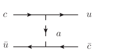
Figure 1: Parton level diagrams for ALP-mediated $D-\bar{D}$ mixing.

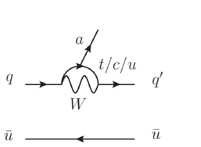
Figure 2: Parton level diagrams for exotic $D$, $K$ and $B$ meson decays involving ALPs.

III.1 $D-\bar{D}$ mixing

The effective Hamiltonian relevant for $D$ meson mixing reads [41]

$$\mathcal{H}_{\rm eff}^{\Delta C=2}=\sum_{i=1}^{5}C_{i}\mathcal{O}_{i}+\sum_{i=1}^{3}\tilde{C}_{i}\tilde{\mathcal{O}}_{i},$$ (25)

where

$$\mathcal{O}_{1} =(\bar{c}_{L}^{\alpha}\gamma^{\mu}u_{L}^{\alpha})(\bar{c}_{L}^{\beta}\gamma_{\mu}u_{L}^{\beta}),$$ (26)

$$\mathcal{O}_{2} =(\bar{c}_{R}^{\alpha}u_{L}^{\alpha})(\bar{c}_{R}^{\beta}u_{L}^{\beta}),\quad\mathcal{O}_{3}=(\bar{c}_{R}^{\alpha}u_{L}^{\beta})(\bar{c}_{R}^{\beta}u_{L}^{\alpha}),$$ (27)

$$\mathcal{O}_{4} =(\bar{c}_{R}^{\alpha}u_{L}^{\alpha})(\bar{c}_{L}^{\beta}u_{R}^{\beta}),\quad\mathcal{O}_{5}=(\bar{c}_{R}^{\alpha}u_{L}^{\beta})(\bar{c}_{L}^{\beta}u_{R}^{\alpha}),$$ (28)

and $\tilde{\mathcal{O}}_{1,2,3}$ are obtained from $\mathcal{O}_{i}$ after exchanging both chiralities, i.e., $L\leftrightarrow R$. Henceforth, we will just be focusing on the new physics contribution to these WCs, i.e., $C_{i}=C_{i}^{\rm NP}$ and $\tilde{C}_{i}=\tilde{C}_{i}^{\rm NP}$. Depending on the specific mass of the ALP, such contributions will involve either short or long-distance physics. The first case occurs when integrating out a heavy enough ALP, $m_{a}\gg m_{c}$, whereas the second one is the consequence of applying naively the operator product expansion (OPE) in powers of $\sim 1/m_{c}$ to the $D-\bar{D}$ system, when $m_{a}\ll m_{c}$. In the first case, one obtains

$$\tilde{C}_{2} =\frac{(c_{u_{R}})_{21}^{2}}{2m_{a}^{2}}\frac{m_{c}^{2}}{f_{a}^{2}},\ C_{2}=\tilde{C}_{2}\frac{m_{u}^{2}}{m_{c}^{2}},\ C_{4}=-2\tilde{C_{2}}\frac{m_{u}}{m_{c}},$$ (29)

and zero elsewhere, while in the second one

$$\tilde{C}_{2} =-\frac{(c_{u_{R}})_{21}^{2}}{2f_{a}^{2}},\ C_{2}=\tilde{C}_{2}\frac{m_{u}^{2}}{m_{c}^{2}},\ C_{4}=-2\tilde{C_{2}}\frac{m_{u}}{m_{c}},$$ (30)

with all other WCs vanishing. In general,

$$2m_{D}M_{12}^{\rm NP} =\sum_{i=1}^{5}C_{i}(\mu)\langle D^{0}|\mathcal{O}_{i}|\bar{D}^{0}\rangle(\mu)$$

$$+\sum_{i=1}^{3}\tilde{C}_{i}(\mu)\langle D^{0}|\tilde{\mathcal{O}}_{i}|\bar{D}^{0}\rangle(\mu),$$ (31)

where $\langle D^{0}|\tilde{\mathcal{O}}_{i}|\bar{D}^{0}\rangle=\langle D^{0}|\mathcal{O}_{i}|\bar{D}^{0}\rangle$, for $i=1,2,3$, due to parity conservation of QCD and $m_{D}=1.865\,$GeV [42]. For small ALP masses, we get [43]

$$|M_{12}^{\rm NP}|=\frac{1}{2m_{D}}\frac{(c_{u_{R}})_{21}^{2}}{2f_{a}^{2}}\,(0.1561\,\mathrm{GeV}^{4}),$$ (32)

where $\langle\mathcal{O}_{2}\rangle=-0.1561\,\mathrm{GeV}^{4}$ at $\mu=3$ GeV, see [43], and we have neglected $\mathcal{O}(m_{u}/m_{c})$ corrections. However, when studying short-distance physics, it is also necessary to run the different WCs from the scale of integration $\Lambda=m_{a}$, to the scale $\mu\sim m_{c}\sim 3\,$GeV. Neglecting $\mathcal{O}(m_{u}/m_{c})$ effects at the UV, we obtain [44]

$$\tilde{C}_{2}(\mu) =\left[r(\mu,\Lambda)^{\frac{1-\sqrt{241}}{6}}\left(\frac{1}{2}-\frac{52}{\sqrt{241}}\right)\right.$$

$$\left.+\,r(\mu,\Lambda)^{\frac{1+\sqrt{241}}{6}}\left(\frac{1}{2}+\frac{52}{\sqrt{241}}\right)\right]\tilde{C}_{2}(\Lambda),$$ (33)

$$\tilde{C}_{3}(\mu) =\frac{705}{32\sqrt{241}}\left[r(\mu,\Lambda)^{\frac{1-\sqrt{241}}{6}}-r(\mu,\Lambda)^{\frac{1+\sqrt{241}}{6}}\right]\tilde{C}_{2}(\Lambda),$$

where

$$r(\mu,\Lambda)=\left(\frac{\alpha_{s}(\Lambda)}{\alpha_{s}(m_{t})}\right)^{2/7}\left(\frac{\alpha_{s}(m_{t})}{\alpha_{s}(m_{b})}\right)^{6/23}\left(\frac{\alpha_{s}(m_{b})}{\alpha_{s}(\mu)}\right)^{6/25}.$$ (34)

Due to the running, to evaluate $M_{12}$ we also need $\langle\mathcal{O}_{3}\rangle$ at $\mu=3\,$GeV, which reads $0.0464\,\mathrm{GeV}^{4}$ [43]. As an example, for $\Lambda=m_{a}=2\,$TeV and $\mu=3\,$GeV, we obtain

$$|M_{12}^{\rm NP}|=\frac{1}{2m_{D}}\frac{(c_{u_{R}})_{21}^{2}}{2f_{a}^{2}}\,(8.95\cdot 10^{-9}\,\mathrm{GeV}^{4}).$$ (35)

We demand that the new physics contribution to $x_{12}=2|M_{12}|/\Gamma$ does not exceed its upper bound at 95% confidence level (CL) [45], i.e.,

$$x_{12}^{\rm NP}=\frac{2|M_{12}^{\rm NP}|}{\Gamma_{D}}<0.63\cdot 10^{-2},$$ (36)

where $\Gamma_{D}=1.60497\cdot 10^{-12}\,\mathrm{GeV}$ [42].

III.2 Exotic D, B and K decays

We study $\Delta F=1$ decays of the form $M\to Na$ with $M=D^{\pm,0},B^{\pm,0},K^{\pm,0}$ and $N=\pi^{\pm,0},K^{\pm,0}$. The corresponding parton level Feynman diagram are shown in fig. 2. The associated matrix element can be decomposed as

$$\langle N(p^{\prime})|\bar{q}_{i}\gamma_{\mu}q_{j}|M(p)\rangle=(p+p^{\prime})_{\mu}f_{+}^{MN}(k^{2})+k_{\mu}f_{-}^{MN}(k^{2})$$

with $k_{\mu}=(p-p^{\prime})_{\mu}$ the momentum transfer and $q_{i}$ and $q_{j}$ the relevant quarks for the decay at the parton level. The scalar form factor is then defined as

$$f_{0}^{MN}(k^{2})=f_{+}^{MN}(k^{2})+\frac{k^{2}}{m_{M}^{2}-m_{N}^{2}}f_{-}^{MN}(k^{2})$$ (38)

and the resulting decay width is given by

$$\Gamma(M\to Na)=\frac{m_{M}^{3}|\varkappa_{MN}|^{2}}{64\pi f_{a}^{2}}\left(1-\frac{m_{N}^{2}}{m_{M}^{2}}\right)^{2}(f_{0}^{MN}(m_{a}^{2}))^{2}$$

$$\times\sqrt{\left(1-\frac{(m_{N}+m_{a})^{2}}{m_{M}^{2}}\right)\left(1-\frac{(m_{N}-m_{a})^{2}}{m_{M}^{2}}\right)},$$ (39)

where $\varkappa_{MN}$ is defined by

$$\mathcal{L}\supset\varkappa_{MN}\frac{\partial^{\mu}a}{2f_{a}}\bar{q}_{i}\gamma_{\mu}q_{j}+\mathrm{h.c.}.$$ (40)

In the model at hand and neglecting small isospin-breaking effects, the exotic $D$ meson decay $D^{\pm,0}\to\pi^{\pm,0}a$ is induced by the dimension-5 operator

$$\mathcal{L}\supset\left(c_{u_{R}}\right)_{ij}\frac{\partial_{\mu}a}{f_{a}}\left(\bar{u}_{R}^{i}\gamma^{\mu}u_{R}^{j}\right).$$ (41)

The width for such decay channel can be read from equation (39) by simply replacing $\varkappa_{MN}$ with $(c_{u_{R}})_{12}$, $m_{M}=m_{D}$, $m_{N}=m_{\pi}$ and using $f_{0}^{D\pi}(m_{a}^{2})$ from [46].

On the other hand, the one-loop running of $c_{u_{R}}$ from the UV scale $f_{a}$ to the IR scale $\mu$ will generate a term 

$$(c_{q_{L}})_{ij}\frac{\partial_{\mu}a}{f_{a}}\left(\bar{q}_{Li}\gamma^{\mu}q_{Lj}\right)$$ (42)

at low energies. Indeed, one obtains [28, 29, 30, 31]

$$16\pi^{2}\frac{d{c_{q_{L}}}}{d\ln\mu} =-\lambda_{u}c_{u_{R}}\lambda_{u}\Rightarrow$$

$$c_{q_{L}} =\frac{\lambda_{u}c_{u_{R}}\lambda_{u}}{32\pi^{2}}\ln\left(\frac{f_{a}^{2}}{\mu^{2}}\right).$$ (43)

After EWSB, this operator leads to

$$\frac{\partial_{\mu}a}{f_{a}}\left[(c_{u_{L}})_{ij}\bar{u}_{Li}\gamma^{\mu}u_{Lj}+(c_{d_{L}})_{ij}\bar{d}_{Li}\gamma^{\mu}d_{Lj}\right],$$ (44)

where $c_{u_{L}}=c_{q_{L}}$ and $c_{d_{L}}=V^{\dagger}c_{q_{L}}V$. More explicitly

$$(c_{d_{L}})_{ij}=\frac{1}{16\pi^{2}v^{2}}V_{ri}^{\ast}(\mathcal{M}_{u})_{rr}(c_{u_{R}})_{rs}(\mathcal{M}_{u})_{ss}V_{sj}\ln\left(\frac{f_{a}^{2}}{\mu^{2}}\right).$$ (45)

This WC is responsible for the exotic decays $B\to Ka$, $B\to\pi a$ and $K\to\pi a$, where $B=B^{\pm,0},K=K^{\pm,0}$ and $\pi=\pi^{\pm,0}$.  The corresponding expressions can be read from equation (39) after taking $\mu\sim m_{t}$ and

$(B\to Ka)$,	$\varkappa_{MN}=(c_{u_{d_{L}}})_{32}$,	$m_{N}=m_{B}$,	$m_{M}=m_{K}$,	$f_{0}^{MN}(m_{a}^{2})=f_{0}^{BK}(m_{a}^{2})$	[47],
$(B\to\pi a)$,	$\varkappa_{MN}=(c_{u_{d_{L}}})_{31}$,	$m_{N}=m_{B}$,	$m_{M}=m_{\pi}$,	$f_{0}^{MN}(m_{a}^{2})=f_{0}^{B\pi}(m_{a}^{2})$	[48],
$(K\to\pi a)$,	$\varkappa_{MN}=(c_{u_{d_{L}}})_{21}$,	$m_{N}=m_{K}$,	$m_{M}=m_{\pi}$,	$f_{0}^{MN}(m_{a}^{2})=f_{0}^{K\pi}(m_{a}^{2})$	[49].

There are no constraints on the branching ratio $\mathrm{Br}(D\to\pi+\mathrm{invisible})$ to date. However, there are measurements of the three-body meson decay $D^{+}\to(\tau^{+}\to\pi^{+}\nu)\bar{\nu}$ [50, 51]. Since these analyses show the event distribution as a function of the missing mass squared $M_{\rm miss}^{2}$ (which would correspond to $m_{a}^{2}$ in the ALP case), one could recast them to constrain the branching ratio $D^{+}\to\pi^{+}a$.  This was done e.g. in [29] for the massless axion by concentrating on the bins with $M_{\rm miss}^{2}\leq 0.05\,\rm{GeV}^{2}$. Since, as we will see, the total width of the ALP in all the benchmarks under consideration is very small, one can safely produce a similar bound for different values of $m_{a}$ by comparing the observed number of events with the predicted background for every bin having $M_{\rm miss}^{2}\geq 0$. More precisely, we derive 90% CL on $\mathrm{BR}(D\to\pi a)$ by using the TLimit class of ROOT [53], which implements the CL_s method [54] and allows to include systematic errors in the background and signal. The bounds arising from [50] turn out to be stronger than those resulting from the use of the more recent experimental analysis in [51].

Regarding exotic meson decays involving down quarks, there are several analysis focused on a massless axion $X^{0}$, like $K^{+}\to\pi^{+}X^{0}$ [55] and $B^{\pm}\to\pi^{\pm}X^{0}$, $B^{\pm}\to K^{\pm}X^{0}$ [56]. There are no searches for a massive ALP $a$, with the exception of the recent analysis in [57], where bounds on $K^{+}\to\pi^{+}a$ as a function of $m_{a}$ were presented. Similarly to the $D^{\pm}\to\pi^{\pm}a$ case, we fill this gap by recasting existing searches on three-body decays, where the relevant kinematic information is provided. In particular, we derive constraints on $B\to Ka$ and $B\to\pi a$ by recasting the searches performed in [58] and [59], respectively. More specifically, we set 90% CL on $B\to Ka$ by combining the observed number of events and the predicted background for $B^{+}\to K^{+}\nu\bar{\nu}$ and $B^{0}\to K^{0}\nu\bar{\nu}$ for every $s_{B}=k^{2}/m_{B}^{2}=m_{a}^{2}/m_{B}^{2}$ bin in figure 5 of [58] with the CL_s method. Finally, for the case of $B\to\pi a$, we derive 90% CL limits on $B\to\pi a$ with the CL_s method by comparing the observed number of events with the predicted background for every $p_{\pi}\equiv\sqrt{\vec{p}_{\pi}^{\,2}}$ bin in the right panel of figure 4 in [59] (which is in one-to-one correspondence with the ALP mass via $m_{a}^{2}=m_{B}^{2}+m_{\pi}^{2}-2m_{B}\sqrt{m_{\pi}^{2}+\vec{p}_{\pi}^{\,2}}$ ).

On the other hand, it is expected that Belle II will be sensitive to the SM $\mathrm{Br}(B^{\pm}\to K^{\pm}\nu\bar{\nu})=(4.0\pm 0.5)\times 10^{-6}$ [60] at 10% accuracy with 50 ab^-1 of data [61], whereas NA62 will measure the branching ratio $\mathrm{Br}(K^{\pm}\to\pi^{\pm}\nu\bar{\nu})$ to within 10% of its SM value $\mathrm{Br}(K^{\pm}\to\pi^{\pm}\nu\bar{\nu})=(8.4\pm 4.1)\times 10^{-11}$ [62, 63]. Regardless of whether these collaborations publish limits directly on a two-body decay or a recast of the three-body decay analysis is needed, such numbers represent a great improvement with respect to current bounds. 

III.3 Radiative $J/\psi$ decays

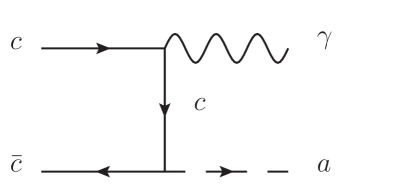
Figure 3: Parton level diagram for the decay $J/\psi\to a\gamma$.

Diagonal ALP couplings to charm quarks are strongly constrained by charmonium decays like $J/\psi\to a\gamma$, as first proposed by [65] and later studied by many others, see e.g. [66, 67, 68, 69, 70, 71]. The parton-level diagram prompting such decay is shown in figure 3. In order to absorb some of the QCD uncertainties of the calculation, it is convenient to normalize the corresponding branching ratio by the one of $J/\psi\to\mu^{+}\mu^{-}$, which is accurately measured $\mathrm{Br}(J/\psi\to\mu^{-}\mu^{+})=5.973$ % [72]. One then obtains

$$\frac{\mathrm{Br}(J/\psi\to a\gamma)}{\mathrm{Br}(J/\psi\to\mu^{-}\mu^{+})}= \frac{G_{F}m_{c}^{2}v^{2}}{\sqrt{2}\pi\alpha_{\rm em}}\left(\frac{(c_{u_{R}})_{22}}{f_{a}}\right)^{2}\times$$

$$\left(1-\frac{m_{a}^{2}}{m_{J/\psi}^{2}}\right)F,$$ (46)

where $F\sim\mathcal{O}(1/2)$ is a correction factor accounting for QCD effects [73, 74], contributions related to bound-state formation [75, 76] as well as relativistic corrections [77]. For the sake of concreteness, we will assume that $F=1/2$ henceforth. This leads to

$$\mathrm{Br}(J/\psi\to a\gamma)=(1.05\,\mathrm{GeV}^{2})\,\left(\frac{(c_{u_{R}})_{22}}{f_{a}}\right)^{2}\left(1-\frac{m_{a}^{2}}{m_{J/\psi}^{2}}\right).$$ (47)

This decay has been searched for by the CLEO collaboration [78], which we will use to constrain the benchmark models at hand.

IV Astrophysical and cosmological bounds

IV.1 Bounds from supernova SN1987a

The observed neutrino burst due to the core-collapse supernova SN1987a can impose constraints on the ALP parameter space. Since neutrino emission constitutes the main cooling mechanism for the proto-neutron star resulting from the collapse, a too large ALP emission could compete with this cooling mechanism and eventually conflict the observed amount of neutrinos. Following [79], we will impose that the ALP luminosity in the proto-neutron star $L_{a}$ does not exceed the neutrino one $L_{\nu}$, i.e., $L_{a}\leq L_{\nu}=3\cdot 10^{52}\,\rm{erg}/s$. 

The ALP luminosity in the proto-neutron star is given by [81, 82]

$$L_{a}=\int_{r\leq R_{\nu}}dV\,\int_{m_{a}}^{\infty}d\omega\,\left(\frac{dP_{a}}{dVd\omega}\right)\,e^{-\tau},$$ (48)

where $\omega$ is the ALP energy and $R_{\nu}\sim\mathcal{O}(40\,\rm{km})$ is the radius of the neutrinosphere, beyond which neutrinos free stream until arriving to the Earth, and we have taken into account the probability $e^{-\tau}$ for an ALP produced within the neutrinosphere to reach $R_{\rm far}\sim\mathcal{O}(100-1000\,\rm{km})$, after which neutrinos are not produced efficiently. If this is not the case, ALPs being produced within the neutrinosphere get ’trapped’ due to their large couplings and their energy is eventually converted back into neutrinos. Such probability is computed with the help of the optical depth $\tau=\tau(m_{a},\omega,r,R_{\rm far})$, for which we will take $R_{\rm far}=100\,\rm{km}$ [81]. In the above expression, $dP_{a}/dVd\omega$ is the ALP differential power. For the charming ALPs considered here, the main channel will be the bremsstrahlung process $N+N\to N+N+a$, since the sole tree-level couplings are those to up-type quarks and therefore to nucleons. Such differential power is given by [79, 83]

$$\frac{dP_{a}}{dVd\omega}=\frac{1}{2\pi^{2}}\omega^{3}\Gamma_{a}e^{-\omega/T}\beta^{2},$$ (49)

where $T$ is the temperature as a function of the radius, $\beta$ is a phase space factor $\beta=\sqrt{1-m_{a}^{2}/\omega^{2}}$ and $\Gamma_{a}$ is the ALP absorption width. The latter is given by

$$\Gamma_{a}=\Gamma_{a}^{pp}+\Gamma_{a}^{nn}+\Gamma_{a}^{pn}+\Gamma_{a}^{np}$$ (50)

with [82]

$$\Gamma_{a}^{NN^{\prime}}=\frac{c_{aNN}^{2}Y_{N}Y_{N^{\prime}}}{4f_{a}^{2}}\frac{\omega}{2}\frac{n_{B}^{2}\sigma_{np\pi}}{\omega^{2}}\gamma_{\rm f}\gamma_{\rm p}\gamma_{\rm h},\quad N^{(\prime)}=n,p.$$ (51)

In the above equation, $c_{aNN}$ is the ALP-nucleon coupling, which reads (see appendix C for more details)

$$c_{app} =(c_{u_{R}})_{11}\left(0.75\pm 0.03\right),$$ (52)

$$c_{ann} =(c_{u_{R}})_{11}\left(-0.51\pm 0.03\right),$$ (53)

while $Y_{N^{(\prime)}}$ is the mass fraction of the nucleon $N^{(\prime)}$, $n_{B}$ is the baryon density, $n_{B}=\rho/m_{N}$, and $\sigma_{np\pi}$ is given by

$$\sigma_{np\pi}=4\alpha_{\pi}^{2}\sqrt{\pi T/m_{N}^{5}},$$ (54)

with $\alpha_{\pi}\approx 15$. For concreteness we take $Y_{p}=0.3$ and $Y_{n}=1-Y_{p}=0.7$. Moreover [84],

$$1/\gamma_{\rm f}=1+\left(n_{B}\sigma_{np\pi}/(2\omega)\right)^{2},$$ (55)

while we use $\gamma_{\rm p}=s(n_{B},Y_{N},\omega/T,m_{\pi}/T)$ with $s$ given by eq. (49) of [85].  On the other hand, following [64], we assume that [86]

$$\gamma_{\rm h}=-0.0726502\ln(\rho)+10^{10}/\rho^{0.9395710}+2.5558616,$$ (56)

where the density $\rho$ is expressed in $\rm{g}\,\rm{cm}^{-3}$. Similarly to [64], we assume for $\rho(r)$ and $T(r)$ and the ”fiducial” profiles of [81]

$$\rho(r)=\rho_{c}\times\left\{\begin{array}[]{ll}1+k_{\rho}(1-r/R_{c})&r<R_{c}\\ (r/R_{c})^{-\nu}&r\geq R_{c}\end{array}\right.,$$ (59)

$$T(r)=T_{c}\times\left\{\begin{array}[]{ll}1+k_{T}(1-r/R_{c})&r<R_{c}\\ (r/R_{c})^{-\nu/3}&r\geq R_{c}\end{array}\right.,$$ (62)

with $k_{\rho}=0.2$, $k_{T}=-0.5$, $\nu=5$, $R_{c}=10\,\rm{km}$, $T_{c}=30$ MeV and $\rho_{c}=3\cdot 10^{14}\,\rm{g}/\rm{cm}^{3}$. We define $R_{\nu}$ as the distance at which the temperature is $3\,$MeV, obtaining $R_{\nu}=39.81\,\rm{km}$. Finally, for the optical depth we take [64]

$$\tau=(R_{\rm far}-R_{\nu})\beta^{-1}\Gamma_{a}(R_{\nu})+\beta^{-1}\int_{r}^{R_{\nu}}d\tilde{r}\,\Gamma_{a}(\tilde{r}).$$ (63)

IV.2 Bounds from red giant burst

The one-loop running of the dimension-5 effective Lagrangian will generate ALP couplings to electrons at low energy. Such couplings face very strong astrophysical bounds for small values of $m_{a}$. This effect can be particularly relevant when the ALP couples to the top quark, since it will contribute significantly to the running [28, 29, 30, 31]:

$$16\pi^{2}\frac{dc_{H}}{d\ln\mu} =-6\mathrm{Tr}\left(\lambda_{u}c_{u_{R}}\lambda_{u}\right)\Rightarrow$$

$$c_{H} =\frac{3}{8\pi^{2}v^{2}}\mathrm{Tr}\left(\mathcal{M}_{u}c_{u_{R}}\mathcal{M}_{u}\right)\ln\left(\frac{f_{a}^{2}}{\mu^{2}}\right),$$ (64)

which leads after field redefinition to

$$-c_{H}\frac{\partial_{\mu}a}{f_{a}}\left(\bar{l}_{Li}\gamma^{\mu}l_{Li}+2\bar{e}_{Ri}\gamma^{\mu}e_{Ri}\right).$$ (65)

After EWSB, these operators lead to

$$\mathcal{L}\supset\frac{ic_{H}a}{f_{a}}m_{\ell}(\bar{\ell}\gamma_{5}\ell)=i\,a\,g_{a\ell\ell}(\bar{\ell}\gamma_{5}\ell),\quad\ell=e,\mu,\tau.$$ (66)

More explicitly, at $\mu\sim m_{t}$,

$$g_{aee}=\frac{c_{H}m_{e}}{f_{a}}=\frac{3m_{e}}{8\pi v^{2}f_{a}}\ln\left(\frac{f_{a}^{2}}{m_{t}^{2}}\right)\sum_{i=1}^{3}\left(\mathcal{M}_{u}\right)_{ii}(c_{u_{R}})_{ii}.$$ (67)

This coupling is bounded by data from red giant bursts [83, 87, 88, 89], $g_{aee}\lesssim 1.6\cdot 10^{-13}$, for ALP masses below the temperature of the red giant.

IV.3 ALP lifetime, branching ratios and cosmological bounds

Cosmological bounds are very sensitive to the total decay width and the different branching ratios of the ALP, that we discuss in the following. We do this both for small values of the ALP mass, where QCD is confined and one can use chiral perturbation theory, as well as for larger values where the dominant ALP decays can be computed using quark-hadron duality [90, 91]. Following [5], we determine the energy scale separating both pictures by demanding that the total decay width to hadrons or SM quarks is of the same order in both regimes, which leads to $\sim 1$ GeV for the benchmark models at hand.

For small masses, $m_{a}\lesssim 1\,$GeV, the ALP decays to two photons via the mixing (18) and the subsequent decay $\pi\to\gamma\gamma$, plus one-loop contributions coming from the integration of heavy quarks. This leads to [18, 21]

$$\Gamma(a\to\gamma\gamma) \approx\frac{\alpha_{\rm em}^{2}m_{a}^{3}}{(4\pi)^{3}f_{a}^{2}}\left|\sum_{i=2}^{3}\frac{4}{3}(c_{u_{R}})_{ii}B_{1}(\tau_{i})\right.$$

$$\left.-\frac{m_{a}^{2}}{2(m_{\pi}^{2}-m_{a}^{2})}(c_{u_{R}})_{11}\right|^{2},$$ (68)

where $B_{1}(\tau_{i})=1-\tau_{i}f^{2}(\tau)$, $\tau_{i}=4(\mathcal{M}_{u})_{ii}^{2}/m_{a}^{2}$, and

$$f(\tau_{i})=\left\{\begin{array}[]{cc}\arcsin(1/\sqrt{\tau_{i}})&\tau_{i}\geq 1\\ \frac{\pi}{2}+\frac{i}{2}\ln\left(\frac{1+\sqrt{1-\tau_{i}}}{1-\sqrt{1-\tau_{i}}}\right)&\tau_{i}<1\end{array}.\right.$$ (69)

This decay channel will be the only one present, whenever the one-loop lepton decays $a\to\ell^{+}\ell^{-}$ are kinematically closed. The leptonic decay widths can be written as

$$\Gamma(a\to\ell^{+}\ell^{-})=\frac{m_{a}m_{\ell}^{2}}{8\pi f_{a}^{2}}\sqrt{1-\frac{4m_{\ell}^{2}}{m_{a}^{2}}}|c_{H}|^{2}.$$ (70)

The diphoton final state will dominate over the $e^{+}e^{-}$ and $\mu^{+}\mu^{-}$ decays in models where $(c_{u_{R}})_{33}$ is absent or negligible. Otherwise, once $a\to e^{+}e^{-}$ and $a\to\mu^{+}\mu^{-}$ open up, they will become the main ALP decay channel, at least for large values of $f_{a}$ leading to log-enhanced $g_{a\ell\ell}$ couplings. At any rate, the $m_{a}^{3}$ dependence of the diphoton decay will make $\Gamma(a\to\gamma\gamma)$ increase faster than the dilepton decay width with increasing values of $m_{a}$. In some cases, this can turn such decay channel into the leading one, once more, for larger ALP masses before $a\to 3\pi$ opens kinematically. Such decay channel will always dominate the $a\to\gamma\gamma$ final state in our models, with its decay width reading [18]

$$\Gamma(a\to\pi^{a}\pi^{b}\pi^{0}) =\frac{\pi}{12}\frac{m_{a}m_{\pi}^{4}}{f_{a}^{2}f_{\pi}^{2}}\left[\frac{(c_{u_{R}})_{11}}{32\pi^{2}}\right]^{2}g_{ab}\left(\frac{m_{\pi}^{2}}{m_{a}^{2}}\right),$$ (71)

with

$$g_{00}(x) =\frac{2}{(1-x)^{2}}\int_{4x}^{(1-\sqrt{x})^{2}}dz\sqrt{1-\frac{4x}{z}}\lambda^{1/2}(1,z,x),$$ (72)

$$g_{+-}(x) =\frac{12}{(1-x)^{2}}\int_{4x}^{(1-\sqrt{x})^{2}}dz\sqrt{1-\frac{4x}{z}}(z-x)^{2}$$

$$\times\lambda^{1/2}(1,z,x),$$ (73)

and $\lambda(a,b,c)=a^{2}+b^{2}+c^{2}-2(ab+ac+bc)$. However, when $(c_{u_{R}})_{33}$ is sizeable and/or $f_{a}$ high enough to have significant $g_{a\ell\ell}$ couplings, $a\to\mu^{+}\mu^{-}$ can be the dominant decay channel in this region of ALP masses.

For masses $m_{a}\gtrsim 1\,$GeV, equation (9) becomes invalid and the dominant ALP decays into hadrons can be computed using quark-hadron duality. The ALP will then decay into gluons and quarks. While the first decay is loop induced, the tree-level decay into quarks will be suppressed by the light Yukawa couplings. Close to threshold, $a\to\bar{q}^{(\prime)}q$ will be the leading decay channel, whereas for larger values of $m_{a}$ $a\to gg$ will take over. In this regime, the $a\to\gamma\gamma$ decay will always be sub-leading and read

$$\Gamma(a\to\gamma\gamma) \approx\frac{\alpha_{\rm em}^{2}m_{a}^{3}}{(4\pi)^{3}f_{a}^{2}}\left|\sum_{i=1}^{3}\frac{4}{3}(c_{u_{R}})_{ii}B_{1}(\tau_{i})\right|^{2}.$$ (74)

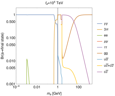
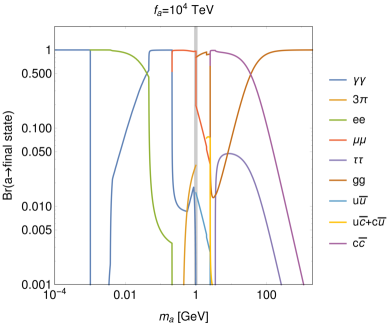
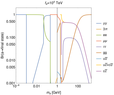
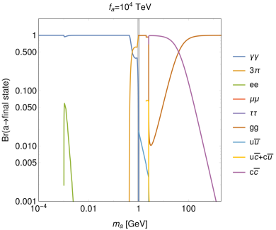
Figure 4: Branching ratios of the ALP as a function of its mass, $m_{a}$, for the different benchmark models. The top panels correspond to the dark-QCD inspired case with $a=\pi_{D_{3}}$ (top left) and $a=\pi_{D_{8}}$ (top right), whereas the bottom panels show the anarchic scenario (bottom left) and the FN motivated benchmark (bottom right), respectively. In all cases, we have assumed $f_{a}=10^{4}$ TeV. Moreover, for the dark-QCD motivated scenarios illustrated in the top panels we have taken $\kappa_{0}=1$. We illustrate with a gray narrow band around 1 GeV, the matching between the calculations performed using chiral perturbation theory and with quark-hadron duality.

We show in figure 4 the different branching ratios for the models at hand for $f_{a}=10^{4}$ TeV, assuming that $\kappa_{0}=1$ in the dark-QCD motivated benchmarks. We can see that in the cases where the ALP coupling to top quarks is absent or suppressed (top-left and bottom-right plots), $a\to\gamma\gamma$ is the leading decay mode for most of the region $m_{a}\lesssim 1$ GeV until $a\to 3\pi$ is kinematically allowed. In the cases where this coupling is present (top-right and bottom-left plots), and for this choice of $f_{a}$, $a\to e^{+}e^{-}$ becomes the leading channel until $a\to\mu^{+}\mu^{-}$ opens up. For ALP masses $\gtrsim 1$ GeV, decays into hadrons are by far the dominant channels, with $a\to gg$ leading at large masses.

Now that we have computed the different branching ratios and lifetimes, we can evaluate the impact of the cosmological constraints. It is important to stress that most of them are derived assuming that $a$ only interacts with photons. However, as discussed in [92], one can apply these cosmological bounds to the more general case where other couplings are present. At the end of the day, we will be able to recast the limits from [92, 93, 94] by using the ALP lifetime $1/\Gamma$, with $\Gamma$ the ALP total decay width. These bounds include the possible impact on $N_{\rm eff}$, potential distortions of the cosmic microwave-background spectrum as well as modifications of the predicted big-bang nucleosynthesis, see [92, 93, 94].

Experiment	distance from IP	length of decay volume	radius/opening angle	$N_{D}$
FASER	480 m	1.5 m	0.1 m	$1.1\times 10^{15}$
FASER2	480 m	5 m	1 m	$2.2\times 10^{16}$
MATHUSLA	68 m downstream,	100 m	25 m high	$2.2\times 10^{16}$
	60 m above
NA62	80 m	65 m	$\theta_{\rm max}=0.05$	$2\times 10^{15}$
SHiP	60 m	50 m	2.5 m	$6.8\times 10^{17}$
CHARM	480 m	35 m	$0.0068<\theta<0.0126$	$4.08\times 10^{15}$

Table 1: Detector parameters for the different fixed-target experiments and LHC forward detectors considered.

Indeed, the bounds can directly be applied when the decay to lepton pairs is dominant, i.e. when there is a sizeable coupling of the ALP with the top quark, provided one interprets $1/\Gamma$ as the total lifetime.  In the cases where $a\to 3\pi$ dominates, bounds from ⁴He overproduction – the dominant constraint in this region – will still hold regardless of the changes in the branching ratios, since only a minimal amount of charged pions is enough for this bound to apply. For even larger masses, ALP decays into hadrons will eventually make its lifetime shorter than a second, making nucleosynthesis constraints harmless. Therefore, even for these masses, we can apply the corresponding bounds if we interpret $\tau$ as the total lifetime.

V Collider probes

V.1 Fixed target experiments

The main production mode for charming ALPs at fixed-target experiments is the decay of $D$ mesons. We consider NA62 [95] and the proposed SHiP experiment [96] as possible detection experiments. We also consider the bounds imposed by the CHARM experiment in [97]. The geometrical outlines of the experiments are listed in table 1.

NA62 operating in beam dump mode, meaning the target is lifted so that the 400 GeV proton beam hits the Cu collimator located 20 m downstream, can be used to search for hidden sector particles [98]. A short run in beam dump mode in November 2016 provided useful information about the backgrounds. It was found that an upstream veto in front of the decay volume could reduce the background to nearly zero [99]. The layout of the SHiP detector is proposed with the aim of reducing the beam-induced backgrounds to 0.1 events [100, 96], so that 3 decay events correspond to the expected exclusion region at over 95% CL.

The total number of dark pions decaying inside the respective decay volume is

$$N_{a}=N_{D}\cdot\mathrm{Br}(D\to\pi a)\cdot\varepsilon_{\rm geom}\cdot F_{\rm decay}\,,$$ (75)

with $\varepsilon_{\rm geom}$ the geometric acceptance, defined as the fraction of ALPs with lab frame momentum at the acceptance angle of the respective detector and $F_{\rm decay}$ the fraction of ALPs that decay inside the decay volume of the respective detector. $F_{\rm decay}$ and $\varepsilon_{\rm geom}$ are calculated following [5]. The $D$ meson momentum distribution for SHiP is taken from [101]. The same distribution is used for the NA62 case as the proton beam is the same.

The CHARM experiment searched for ALPs decaying into pairs of photons, electrons and muons. In [97] no events where found, so that we set a bound at 90% CL at $N_{\rm obs}=2.3$ events [102]. We assume that for our model the main production channel for ALPs is the decay $D^{\pm}\to\pi^{\pm}a$. CHARM also has a 400 GeV proton beam, so we again use the same momentum distribution for the $D$ mesons. The number of protons on target is $2.4\times 10^{18}$ [97] and such a proton beam has a probability of $1.7\times 10^{-3}$ to produce a pair of $c$ quarks [103], leading to $4.08\times 10^{15}$ produced $D$ mesons. Multiplying eq. (75) by $\sum_{i=\gamma,e,\mu}Br(a\to ii)$ to take into account that in [97] only the $\gamma\gamma$, $ee$ and $\mu\mu$ final states were searched for we use the same procedure as for NA62 and SHiP to impose the 90% CL bound from CHARM.

V.2 LHC forward detectors

FASER [104] and the proposed MATHUSLA detector [105, 106] are designed to detect long-lived particles produced in proton-proton collisions at LHC. Hadron collisions have the advantage of additional production modes, such as production via gluon fusion. The detector parameters are given in table 1. We focus again on the production via $D$ meson decays. The meson momentum distribution was simulated using FONLL with CTEQ6.6 [107]. As for SHiP and NA62 the number of dark pions decaying inside the decay volume can be calculated using eq. (75). For LHC run-3 $N_{D}=1.1\times 10^{15}$, which increases by a factor 20 at the High Luminosity (HL)-LHC. FASER will operate at LHC run-3, while FASER2 and MATHUSLA are under consideration for the HL-LHC. Following the procedure as described for SHiP and NA62 the number of dark pions decaying inside FASERs, FASER2s and MATHUSLAs decay volume is calculated. At least three events must decay inside the respective decay volume for a discovery.

VI Results

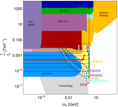
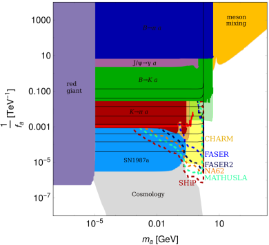
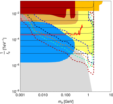
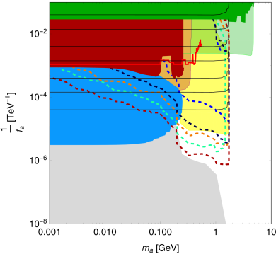
Figure 5: Experimental constraints and expected bounds on $1/f_{a}$ as a function of $m_{a}$ for the dark-QCD inspired models. Left panels correspond to the case $a=\pi_{D}^{3}$, while right panels illustrate the scenario $a=\pi_{D}^{8}$. Light green and light red areas correspond to the expected constraints coming from Belle II and NA62, respectively. We show by a red line the constraints arising from the recast of the three-body decay $D^{+}\to(\tau^{+}\to\pi^{+}\bar{\nu})\nu$, whereas the impact of a direct measurement of $\mathrm{Br}(D\to\pi a)$ is represented by black lines, with values going from $10^{-1}$ to $10^{-8}$, each one a decade smaller. Dashed lines correspond to different fix-target experiments and collider probes of the model, see the main text for more details. Lower panels zoom in the regions where upcoming experiments are sensitive. In order to evaluate the logarithms coming from the one-loop running we further assume $\kappa_{0}=1$.

The resulting constraints on the parameter space of the four benchmarks models under consideration are displayed in figures 5 and 6. More specifically, we show in figure 5 the different bounds for the dark-QCD motivated benchmarks, with left panels corresponding to the case $a=\pi_{D_{3}}$ and the right ones to $a=\pi_{D_{8}}$, respectively. For these two benchmarks we further assume $\kappa_{0}=1$ in order to evaluate the logarithms coming from the one-loop running, which only depend on $f_{a}$. Still, different choices of $\kappa_{0}\sim\mathcal{O}(1)$ will not significantly affect the resulting bounds shown in the figure. On the other hand, we show in figure 6 the corresponding bounds for the anarchic (left panels) and FN (right panels) scenarios.

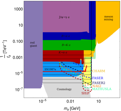
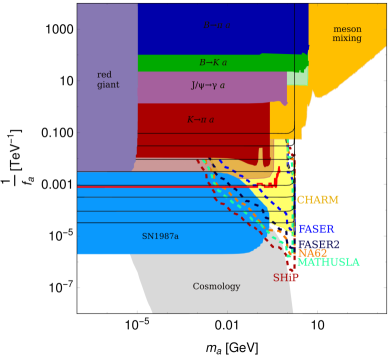
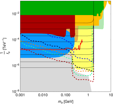
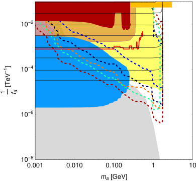
Figure 6: Same as figure 5 but for the anarchic and the FN inspired models, left and right panels, respectively. Lower panels zoom in the regions where upcoming experiments are sensitive.

In both figures, we represent in dark yellow the region of the parameter space excluded by $D$ meson mixing, whereas the bounds from exotic meson decays $B\to Ka$, $B\to\pi a$ and $K\to\pi a$ are displayed in green, blue and red, respectively. Moreover, for the sake of illustration, one can roughly interpret the expected bounds on $B\to K\nu\bar{\nu}$ from Belle II as sensitivity to $B\to Ka$, which we show in light green. Similarly, one could do the same thing in the case of $K\to\pi\nu\bar{\nu}$ from NA62, which is represented in light red. A proper recast of these two upcoming experimental results will most likely result in slightly weaker bounds. On the other hand, we show the limits arising from the recast of $D^{+}\to(\tau^{+}\to\pi^{+}\nu)\bar{\nu}$ as a red line. Finally, we show in purple the bounds resulting from $J/\psi\to a\gamma$ searches by the CLEO collaboration. The cosmological bounds discussed previously are shown in gray in both figures, with the constraints arising from red giant bursts and from SN1987a exhibited in lilac and light blue, respectively.

The region where the ALP mass lies above the $D$ and $B$ meson masses is only weakly constrained by flavour observables, and is open for probes at the energy frontier, i.e. the LHC and future colliders. Below the $D$ meson mass, some viable regions remain which can be probed by the upcoming or proposed collider experiments discussed in section V. The projected bounds from SHiP and NA62 are represented by dark red and orange dashed contours, respectively. Above these lines more than three events are expected. Furthermore, the discovery lines for FASER with LHC run-3 and FASER2 at HL-LHC are displayed in dashed light and dark blue, respectively, whereas the detection line for MATHUSLA is pictured as a turquoise dashed contour line.

In order to appreciate better the region which can be probed by these upcoming experiments, we show in the lower panels of figures 5 and 6 a zoomed-in view of the area which may be reached. While FASER will mainly validate the constraints from the CHARM experiment shown in light yellow, FASER2 at the HL-LHC as well as NA62 will probe new regions of parameter space, with SHiP and MATHUSLA covering the remaining unexplored areas below the charm mass threshold.

A possible measurement of $\mathrm{Br}(D\to\pi+\rm{invisible})$ could provide a complementary test of these parts of the parameter space, and might be crucial to probe the region close to the charm mass at relatively large coupling. In the FN inspired model as well as the $\pi_{D}^{3}$ scenario this region of parameter space is not otherwise accessible, while in the $\pi_{D}^{8}$ scenario it will be probed by Belle II, and in the anarchic case it is already excluded. Similarly, the low mass region of the $\pi_{D}^{3}$ scenario is only accessible via $\mathrm{Br}(D\to\pi+\rm{invisible})$ and future NA62 measurements. To display the discovery potential of such a measurement, we show black contour lines corresponding to values of $\mathrm{Br}(D^{\pm}\to\pi^{\pm}\rm{invisible})\in\{10^{-8},\,10^{-7},\,10^{-6},\,10^{-5},\,10^{-4},\,10^{-3},\,10^{-2},\,10^{-1}\}$. This demonstrates that providing an experimental measurement of the exotic meson decay $D\to\pi a$ is paramount to leave no stone unturned in the quest for well motivated extensions of the SM that feature charming ALPs.

VII Conclusions

In this work we have presented several examples of models featuring charming ALPs, i.e., light pNGBs having off-diagonal couplings with SM up-quarks, and studied in detail the phenomenology associated with their low-energy EFTs. More specifically, we have studied the constraints arising from flavour experiments, astrophysics and cosmology as well as planned fixed-target and collider experiments in four benchmark models. We have shown that such scenarios have still a large unexplored parameter space. We have also demonstrated how future collider and fixed-target experiments can probe these models and that they could be perfectly complemented by the measurement of the exotic decay $D\to\pi+\rm{invisible}$, which is currently unavailable. We thus encourage our experimental colleagues to proceed with such measurement. In the absence of dedicated searches, we have also derived bounds on the parameter space of the models by recasting three-body meson decays like $D^{+}\to(\tau^{+}\to\pi^{+}\nu)\bar{\nu}$ or $B\to K/\pi\,\nu\bar{\nu}$.

The scenarios considered here can be the low-energy EFT of several compelling UV completions. We have presented two of them: the case of a QCD-like dark sector interacting with the SM via a heavy scalar mediator with hypercharge $-2/3$, and a FN model of flavour where only RH up-quarks and a heavy scalar have non-zero charges with respect to an spontaneously broken global $U(1)$ symmetry. Some of the phenomenology studied here may change when considering the whole picture in the dark-QCD case, since there might be a non-trivial interplay between the complete set of pNGBs in some regions of the parameter space. In the present work, we have focused on the phenomenological aspects expected to hold when singling out one of such light states. The complete dark-QCD model will be studied in an upcoming work, where a detailed study of the full charming dark sector including the possible connection with dark matter will be presented. A particularly interesting aspect of such scenarios to be studied is the collider phenomenology involving rare top decays $t\to ca$ as well as the phenomenology of ’charming’ emerging jets.

A final region of parameter space that was left unexplored in our study is that of very small ALP masses and couplings, i.e. the lower left regions of our figures. There the charming ALP would be a stable dark matter (DM) candidate. The freeze-out of such a DM candidate is excluded for $m_{a}\gtrsim 100$ eV due to DM overproduction  [92] and in the whole parameter region if structure formation bounds are also taken into account  [108]. On the other hand, if the charming ALP DM is produced via a ”freeze-in” mechanism, a region of parameter space remains viable [108] in principle. A more detailed exploration of this region of the charming ALP is left for future work.

Appendix A A dark QCD UV completion

One particular class of theories which can provide a UV completion to the charming ALP EFT is what can be collectively denoted by ’dark QCD’, see e.g. [11, 12, 5]. In these scenarios, one assumes that the SM is extended with a new dark QCD-like gauge group $SU(N_{d})_{d}$ with $n_{d}$ Dirac fermions, $Q_{\alpha},\,\alpha=1,\ldots,n_{d}$, singlets of the SM gauge group and transforming in the fundamental representation of $SU(N_{d})_{d}$. For concreteness one can assume $N_{d}=3=n_{d}$, which allows in particular the QCD-like sector to confine at a scale $\Lambda_{d\rm QCD}$. Both sectors talk to each other through the coupling to a heavy scalar mediator, $\mathcal{X}$, transforming as a $(\mathbf{3},\bar{\mathbf{3}})$ under $SU(3)\otimes SU(3)_{d}$, which is also charged under $SU(2)_{L}\otimes U(1)_{Y}$ as $\mathbf{1}_{-2/3}$. Such scalar mediator is naturally heavy, also in agreement with LHC bounds. A similar setup was presented first in [11] but with a different assignment of hypercharge, $Y=1/3$, such that only couplings to RH down-like quarks were allowed. It was shown in [12, 12, 5] that this scenario lead to emerging jets and its flavour phenomenology was studied in [5]. Here, we focus on a different hypercharge assignment, which leads to a distinct phenomenology. The structure of the model is sketched in figure 7.

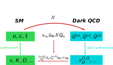
Figure 7: Schematic illustration of the high-energy and low-energy regimes of the dark QCD UV completion.

The Lagrangian of the dark sector reads

$$\mathcal{L}_{D} =-\frac{1}{4}\mathcal{G}_{d}^{\mu\nu,a}\mathcal{G}^{d,a}_{\mu\nu}+\bar{Q}_{\alpha}i\cancel{D}Q_{\alpha}-m_{Q\alpha,\beta}\bar{Q}_{\alpha}Q_{\beta}$$

$$+|D_{\mu}\mathcal{X}|^{2}-m_{\mathcal{X}}^{2}|\mathcal{X}|^{2}-\left[\kappa_{\alpha i}\bar{u}_{Ri}\mathcal{X}Q_{\alpha}+\mathrm{h.c.}\right],$$ (76)

where we use greek (latin) indices to denote the flavour indices in the dark (visible) QCD sector and we do not need to explicitly write the corresponding covariant derivatives. Similarly, we did not make explicit color or dark color indices with the exception of $\mathcal{G}_{\mu\nu}^{a}$, $a=1,\ldots,8$, the field-strength tensor for the dark QCD. In general, the coupling matrix $\kappa_{\alpha i}$ can be expressed as

$$\kappa=VDU$$ (77)

where both $U$ and $V$ are $3\times 3$ unitary matrices and $D$ is a $3\times 3$ diagonal matrix. In the case where $m_{Q\alpha\beta}=m_{Q}\delta_{\alpha\beta}$, there is a $U(3)_{d}$ flavour symmetry in the dark sector, which can be used to rotate away $V$. We will assume that this is the case henceforth. The matrix $U$ can be further expressed as the following product

$$U=U_{23}U_{13}U_{12},$$ (78)

where $U_{ij}$ are unitary rotations between the flavours $i$ and $j$. For example, $U_{12}$ reads

$$U_{12}=\begin{pmatrix}c_{12}&s_{12}e^{-i\delta_{12}}&0\\ -s_{12}e^{-i\delta_{12}}&c_{12}&0\\ 0&0&1\end{pmatrix},$$ (79)

where $c_{12}=\cos\theta_{12}$, $s_{12}=\sin\theta_{12}$. Moreover, following [2, 5] one can express $D$ as

$$D=\mathrm{diag}\left(\kappa_{0}+\kappa_{1},\kappa_{0}+\kappa_{2},\kappa_{0}-(\kappa_{1}+\kappa_{2})\right),$$ (80)

where $\kappa_{0}\geq|\kappa_{1}+\kappa_{2}|$. For the sake of concreteness, we will consider the benchmark model defined by

$$\kappa_{1}=\kappa_{0}/2,\quad\kappa_{2}=0,\quad\theta_{13}=\theta_{23}=0,\quad\delta_{ij}=0,\,\forall i,j.$$ (81)

We also assume that all this happens in a basis where the SM up Yukawa matrix is diagonal.

If the mass of scalar mediator is much heavier than $\Lambda_{d\rm QCD}$ and $\Lambda_{\rm QCD}$, one gets in addition to the SM Lagrangian

$$\mathcal{L}_{\mathrm{eff}} =-\frac{1}{4}\mathcal{G}_{d}^{\mu\nu,a}\mathcal{G}^{d,a}_{\mu\nu}+\bar{Q}_{\alpha}i\cancel{D}Q_{\alpha}-m_{Q}\bar{Q}_{\alpha}Q_{\alpha}$$

$$-\frac{\kappa_{\alpha i}\kappa^{\ast}_{\beta j}}{2m_{\mathcal{X}}^{2}}\left(\bar{Q}_{\beta}\gamma_{\mu}P_{L}Q_{\alpha}\right)(\bar{u}_{Ri}\gamma^{\mu}u_{Rj}),$$ (82)

after integrating out $\mathcal{X}$ and using Fierz identities. Similarly to QCD, in the limit $m_{Q}\to 0$ and $m_{\mathcal{X}}\to\infty$, the dark sector features a global dark chiral symmetry $SU(3)_{dL}\otimes SU(3)_{dR}$, which we assume is spontaneously broken to its diagonal group $SU(3)_{dV}$ by the dark QCD condensate $\langle\bar{Q}_{\alpha}Q_{\beta}\rangle\propto\delta_{\alpha\beta}\Lambda_{d\rm QCD}^{3}$. This spontaneous symmetry breaking delivers 8 Nambu-Goldstone bosons, $\pi_{D_{1}},\ldots,\pi_{D_{8}}$, which will become pNGBs once we switch on $m_{Q}$. We will consider the case where $m_{Q}\ll\Lambda_{d\rm QCD}$ so that the pNGBs are parametrically lighter than the rest of particles in the spectrum. With the exception of the lightest baryonic bound states carrying a conserved dark baryon number, the rest of the particles of the spectrum will undergo fast decays to dark pions. Therefore, it is a reasonable approximation to just consider such dark pions. In the case at hand where $n_{d}=3=N_{d}$, one can write down an effective theory for the resulting eight pNGBs along the lines of the QCD case of pions and kaons. Using the basis of Gell-Mann matrices, $\lambda^{a}$, $a=1,\ldots,8$, one can write

$$\Pi_{D} =\pi_{D_{a}}\frac{\lambda^{a}}{2}$$ (83)

$$=\frac{1}{2}\begin{pmatrix}\pi_{D_{3}}+\frac{\pi_{D_{8}}}{\sqrt{3}}&\pi_{D_{1}}-i\pi_{D_{2}}&\pi_{D_{4}}-i\pi_{D_{5}}\\ \pi_{D_{1}}+i\pi_{D_{2}}&-\pi_{D_{3}}+\frac{\pi_{D_{8}}}{\sqrt{3}}&\pi_{D_{6}}-i\pi_{D_{7}}\\ \pi_{D_{4}}+i\pi_{D_{5}}&\pi_{D_{6}}+i\pi_{D_{7}}&-\frac{2}{\sqrt{3}}\pi_{D_{8}}\end{pmatrix}.$$

The corresponding Goldstone matrix transforming non-linearly under $SU(3)_{dL}\otimes SU(3)_{dR}$ and linearly under $SU(3)_{dV}$ can be written as

$$U_{D}(\Pi_{D})=\mathrm{exp}\left(\frac{2i}{f_{d}}\Pi_{D}\right),$$ (84)

where $f_{d}$ is the dark pion decay constant, in principle a free parameter. In analogy to chiral perturbation theory (ChPT) for QCD, the Lagrangian describing the dark pions in the absence of interaction with the SM is given by

$$\mathcal{L}_{d\rm ChPT} =\frac{f_{d}^{2}}{4}\mathrm{Tr}\left(\partial_{\mu}U_{D}\partial^{\mu}U^{\dagger}_{D}\right)$$

$$+\frac{f_{d}^{2}B_{D}}{2}m_{Q}\mathrm{Tr}\left(U_{D}^{\dagger}+U_{D}\right),$$ (85)

where $B_{d}$ is a constant related to the dark pion mass. More precisely

$$m_{\pi_{D_{a}}}^{2}=m_{\pi_{D}}^{2}=2m_{Q}B_{d}.$$ (86)

As one can see, they are all degenerate in mass, but small splittings will be induced by their interactions with the SM. Such radiative corrections will define new mass eigenstates

$$\pi^{(1,2)}_{D} =\frac{1}{\sqrt{2}}\left(\pi_{D_{1}}-i\pi_{D_{2}}\right),$$ (87)

$$\pi^{(1,3)}_{D} =\frac{1}{\sqrt{2}}\left(\pi_{D_{3}}-i\pi_{D_{4}}\right),$$ (88)

$$\pi^{(2,3)}_{D} =\frac{1}{\sqrt{2}}\left(\pi_{D_{6}}-i\pi_{D_{7}}\right),$$ (89)

with $\pi_{D_{3}}$ and $\pi_{D_{8}}$ unchanged.

If the dark pions are light enough, $m_{\pi_{D}}\lesssim 4\pi f_{\pi}$, their decays are better described by ChPT for the SM quarks. The part containing only SM fields is described by

$$\mathcal{L}_{\rm ChPT}=\frac{f_{\pi}^{2}}{4}\mathrm{Tr}\left(\partial_{\mu}U\partial^{\mu}U^{\dagger}\right)+\frac{f_{\pi}^{2}B_{0}}{2}\mathrm{Tr}\left(m_{q}U^{\dagger}+Um_{q}^{\dagger}\right),$$ (90)

whereas the interaction with the dark QCD sector is described by

$$\mathcal{L}_{\rm ChPT}^{\rm mix} =-\frac{f_{d}^{2}f_{\pi}^{2}}{2m_{\mathcal{X}}^{2}}\kappa_{\alpha i}\kappa^{\ast}_{\beta j}\mathrm{Tr}\left(c_{\beta\alpha}U_{D}^{\dagger}\left(\partial_{\mu}U_{D}\right)\right)\times$$

$$\mathrm{Tr}\left(c_{ij}U\left(\partial^{\mu}U\right)^{\dagger}\right),$$ (91)

where the projection matrices $c_{\alpha\beta}$ and $c_{ij}$ are defined as

$$c_{\alpha\beta}^{mn}=\delta_{\alpha}^{m}\delta_{n}^{\beta},\quad\alpha,\beta=1,2,3,\quad c_{ij}^{mn}=\delta_{i}^{m}\delta_{j}^{n},\quad i,j=1,$$ (92)

being zero otherwise. For larger dark pion masses, one can use quark-hadron duality [90, 91], with the relevant Lagrangian being

$$\mathcal{L}_{\rm mix}=i\frac{f_{d}^{2}}{2m_{\mathcal{X}}^{2}}\kappa_{\alpha i}\kappa^{\ast}_{\beta j}\mathrm{Tr}\left(c_{\beta\alpha}U_{D}^{\dagger}\left(\partial_{\mu}U_{D}\right)\right)(\bar{u}_{Ri}\gamma^{\mu}u_{Rj}).$$ (93)

For the benchmark model at hand, only $\pi_{D_{3}},\pi_{D_{8}}$ and $\pi_{D}^{(1,2)}$ decay at tree-level. The rest of dark pions, which decay through loop-induced processes, are therefore long-lived. For this reason, we focus on the first dark pions, and in particular, on the two real ones $\pi_{D_{3}}$ and $\pi_{D_{8}}$.  In particular, the mixing terms in eqs. (91) and (93) involving $\pi_{D_{3}}$ and $\pi_{D_{8}}$ read

$$\mathcal{L}_{\rm ChPT}^{\rm mix} \supset-\frac{f_{d}f_{\pi}^{2}}{2m_{\mathcal{X}}^{2}}\sum_{a=3,8}\sum_{\alpha\beta}\kappa_{\alpha i}\kappa^{\ast}_{\beta j}\left(\lambda^{a}\right)_{\alpha\beta}\partial_{\mu}\pi_{D_{a}}\times$$

$$\mathrm{Tr}\left(c_{ij}U\left(\partial^{\mu}U\right)^{\dagger}\right)$$ (94)

and

$$\mathcal{L}_{\rm mix}\supset-\frac{f_{d}}{2m_{\mathcal{X}}^{2}}\sum_{a=3,8}\sum_{\alpha\beta}\kappa_{\alpha i}\kappa^{\ast}_{\beta j}\left(\lambda^{a}\right)_{\alpha\beta}\partial_{\mu}\pi_{D_{a}}(\bar{u}_{Ri}\gamma^{\mu}u_{Rj}),$$ (95)

respectively. Comparing these equations with the mixing terms present in eqs. (1) and (9) for $a=\pi_{D_{3}}$ and $\pi_{D_{8}}$, respectively, we obtain $f_{a}=m_{\mathcal{X}}^{2}/f_{d}$ and

$$(c_{u_{R}}^{(a)})_{ij}=-\sum_{\alpha\beta}\kappa_{\alpha i}\kappa^{\ast}_{\beta j}\left(\lambda^{a}\right)_{\alpha\beta},\qquad a=3,8.$$ (96)

More explicitly,

$$c_{u_{R}}^{(3)} =\frac{\kappa_{0}^{2}}{4}\begin{pmatrix}4s_{12}^{2}-9c_{12}^{2}&-13c_{12}s_{12}&0\\ -13c_{12}s_{12}&4c_{12}^{2}-9s_{12}^{2}&0\\ 0&0&0\end{pmatrix},$$ (97)

$$c_{u_{R}}^{(8)} =\frac{-\kappa_{0}^{2}}{4\sqrt{3}}\begin{pmatrix}4s_{12}^{2}+9c_{12}^{2}&5c_{12}s_{12}&0\\ 5c_{12}s_{12}&4c_{12}^{2}+9s_{12}^{2}&0\\ 0&0&-2\end{pmatrix}.$$ (98)

Appendix B A Froggatt-Nielsen UV completion

Another motivation for the ALPs considered here corresponds to what is generically known by the name of flavons or familions (see [109, 110, 111, 112, 113, 87] and e.g. [114, 115, 116, 117, 118, 119, 120, 121, 122, 123] for more recent implementations), pNGBs of some spontaneously broken flavour symmetry, which may be anomalous, and that generically feature flavour-violating couplings to quarks or leptons. One particular setup leading to the scenario we have in mind, i.e., the effective Lagrangian (1) in addition to $c_{H}=0$, is given by FN models when only RH up-quarks have non-zero charges. Specifically, one considers a global $U(1)$ flavour symmetry, spontaneously broken by the vacuum expectation value of some extra scalar $\langle S\rangle=f_{a}$, where

$$S=\frac{1}{\sqrt{2}}(f_{a}+s)e^{ia/f_{a}},$$ (99)

and has charge $-1$ under this new $U(1)$. If only $u_{Ri}$ are charged under such global symmetry, with charges $n_{i}^{u}$, Yukawa couplings for up-quarks will be higher-dimensional

$$\mathcal{L}\supset-(y_{u})_{ij}\left(\frac{S}{\Lambda}\right)^{n_{j}^{u}}q_{Li}\tilde{H}u_{Rj}+\mathrm{h.c.},$$ (100)

where one typically assumes that $f_{a}<\Lambda$. At the end of the day, such term in the Lagrangian will generate interactions like (4)

$$-\frac{ia}{f_{a}}\bar{q}_{Li}\tilde{H}u_{Rj}n_{j}^{u}=-\frac{ia}{f_{a}}\bar{q}_{Li}\tilde{H}u_{Rj}(Y_{u})_{ij}n_{j}^{u},$$ (101)

where $Y_{u}$ is the effective up Yukawa matrix,

$$(Y_{u})_{ij}=(y_{u})_{ij}\left(\frac{f_{a}}{\Lambda}\right)^{n_{j}^{u}}.$$ (102)

If we assume that $(y_{u})_{ij}=\mathcal{O}(1)$ and take $f_{a}/\Lambda=\epsilon\sim m_{c}/m_{t}$, we can get the correct up quark masses by choosing $n_{u}=(2,1,0)$ since

$$(m_{u},m_{c},m_{t})\sim\frac{1}{\sqrt{2}}v\,(\epsilon^{2},\epsilon,1)$$ (103)

and

$$\frac{m_{u}}{m_{t}}\sim\epsilon^{2},\qquad\frac{m_{c}}{m_{t}}\sim\epsilon.$$ (104)

In this case, we can diagonalize $Y_{u}$ by making

$$u_{R}\to U_{R}^{u}u_{R},\qquad u_{L}\to U_{L}^{u}u_{L},$$ (105)

with

$$U_{R}^{u}\sim\begin{pmatrix}1&\epsilon&\epsilon^{2}\\ \epsilon&1&\epsilon\\ \epsilon^{2}&\epsilon&1\end{pmatrix},\qquad(U_{L}^{u})_{ij}\sim\mathcal{O}(1).$$ (106)

This leads, after going to the basis where $Y_{u}$ is diagonal to

$$c_{u_{R}}\sim\begin{pmatrix}2&3\epsilon&3\epsilon^{2}\\ 3\epsilon&1&\epsilon\\ 3\epsilon^{2}&\epsilon&\epsilon^{2}\end{pmatrix}.$$ (107)

This sentence is here to fix the layout.

Appendix C ALP couplings to nucleons

The leading order ALP couplings with nucleons can be read from the following Lagrangian [124, 125, 34, 126]

$$\mathcal{L}_{\rm int} =\left(\frac{\partial_{\mu}a}{4f_{a}}\right)\Big{\{}\mathrm{Tr}\left((\hat{c}+\varkappa_{q}c_{g})\lambda^{a}\right)\left(F\,\mathrm{Tr}\left(\bar{B}\gamma^{\mu}\gamma_{5}\left[\lambda^{a},B\right]\right)+D\,\mathrm{Tr}\left(\bar{B}\,\gamma^{\mu}\gamma_{5}\left\{\lambda^{a},B\right\}\right)\right)$$

$$+ \frac{1}{3}\mathrm{Tr}\left(\hat{c}+\varkappa_{q}c_{g}\right)\,S\,\mathrm{Tr}\left(\bar{B}\,\gamma^{\mu}\gamma_{5}B\right)+\mathrm{Tr}\left((\hat{c}+\varkappa_{q}c_{g})\lambda^{a}\right)\mathrm{Tr}\left(\bar{B}\,\gamma^{\mu}\left[\lambda^{a},B\right]\right)\Big{\}}$$ (108)

where $B$ is the baryon matrix

$$B=\frac{1}{\sqrt{2}}B^{a}\lambda^{a}=\begin{pmatrix}\frac{\Sigma^{0}}{\sqrt{2}}+\frac{\Lambda}{\sqrt{6}}&\Sigma^{+}&p\\ \Sigma^{-}&-\frac{\Sigma^{0}}{\sqrt{2}}+\frac{\Lambda}{\sqrt{6}}&n\\ \Xi^{-}&\Xi^{0}&-\frac{2\Lambda}{\sqrt{6}}\end{pmatrix},$$ (109)

and the axial-vector coupling constants $F$ and $D$ are defined by

$$\langle B^{\prime}_{i}|J_{j}^{(8)}|B_{k}\rangle=if_{ijk}F+d_{ijk}D,$$ (110)

with $J_{j}^{(8)}$ the weak axial-vector hadronic current, transforming as an $SU(3)$ octet, $f_{ijk}$ the totally antisymmetric structure constants of $SU(3)$ and $d_{ijk}$ the totally symmetric ones. On the other hand, $S$ is defined by the singlet current which can be renormalized independently. $D$ and $F$ can be determined by hyperon semileptonic decays [127], leading to $F=0.463\pm 0.008$, $D=0.804\pm 0.008$. On the other hand $S\approx 0.13\pm 0.2$ [128]. We are particularly interested in the $a\bar{N}N$ couplings, with $N=p,n$, which read

$$\mathcal{L}_{\rm int}\supset\frac{1}{12}\frac{\partial_{\mu}a}{f_{a}}\left(c_{u_{R}}\right)_{11}\Big{(}\big{[}S-4D\big{]}(\bar{n}\gamma^{\mu}\gamma_{5}n)+\big{[}2D+6F+S\big{]}(\bar{p}\gamma^{\mu}\gamma_{5}p)+6\bar{p}\gamma^{\mu}p\Big{)}$$ (111)

The last term in the equation above is a total derivative which can be neglected. In this case

$$\mathcal{L}_{aNN}=\sum_{N=p,n}\frac{\partial_{\mu}a}{2f_{a}}c_{aNN}\bar{N}\gamma^{\mu}\gamma_{5}N$$ (112)

with

$$c_{app} =(c_{u_{R}})_{11}\left(F+\frac{1}{3}D+\frac{1}{6}S\right)=(c_{u_{R}})_{11}\left(0.75\pm 0.03\right),$$ (113)

$$c_{ann} =(c_{u_{R}})_{11}\left(\frac{1}{6}S-\frac{2}{3}D\right)=(c_{u_{R}})_{11}\left(-0.51\pm 0.03\right).$$ (114)

References

- [1] N. Craig, A. Katz, M. Strassler and R. Sundrum, Naturalness in the Dark at the LHC, JHEP 07 (2015) 105 [1501.05310].
- [2] P. Agrawal, M. Blanke and K. Gemmler, Flavored dark matter beyond Minimal Flavor Violation, JHEP 10 (2014) 072 [1405.6709].
- [3] B. Batell, J. Pradler and M. Spannowsky, Dark Matter from Minimal Flavor Violation, JHEP 08 (2011) 038 [1105.1781].
- [4] L. Calibbi, A. Crivellin and B. Zaldívar, Flavor portal to dark matter, Phys. Rev. D 92 (2015) 016004 [1501.07268].
- [5] S. Renner and P. Schwaller, A flavoured dark sector, JHEP 08 (2018) 052 [1803.08080].
- [6] H. Mies, C. Scherb and P. Schwaller, Collider constraints on dark mediators, 2011.13990.
- [7] M. Blanke and S. Kast, Top-Flavoured Dark Matter in Dark Minimal Flavour Violation, JHEP 05 (2017) 162 [1702.08457].
- [8] T. Jubb, M. Kirk and A. Lenz, Charming Dark Matter, JHEP 12 (2017) 010 [1709.01930].
- [9] M. Blanke, P. Pani, G. Polesello and G. Rovelli, Single-top final states as a probe of top-flavoured dark matter models at the LHC, 2010.10530.
- [10] M. J. Strassler and K. M. Zurek, Echoes of a hidden valley at hadron colliders, Phys. Lett. B 651 (2007) 374 [hep-ph/0604261].
- [11] Y. Bai and P. Schwaller, Scale of dark QCD, Phys. Rev. D89 (2014) 063522 [1306.4676].
- [12] P. Schwaller, D. Stolarski and A. Weiler, Emerging Jets, JHEP 05 (2015) 059 [1502.05409].
- [13] H.-C. Cheng, L. Li, E. Salvioni and C. B. Verhaaren, Light Hidden Mesons through the Z Portal, JHEP 11 (2019) 031 [1906.02198].
- [14] C. D. Froggatt and H. B. Nielsen, Hierarchy of Quark Masses, Cabibbo Angles and CP Violation, Nucl. Phys. B147 (1979) 277.
- [15] J. Jaeckel and M. Spannowsky, Probing MeV to 90 GeV axion-like particles with LEP and LHC, Phys. Lett. B 753 (2016) 482 [1509.00476].
- [16] I. Brivio, M. B. Gavela, L. Merlo, K. Mimasu, J. M. No, R. del Rey et al., ALPs Effective Field Theory and Collider Signatures, Eur. Phys. J. C77 (2017) 572 [1701.05379].
- [17] B. Bellazzini, A. Mariotti, D. Redigolo, F. Sala and J. Serra, -axion at colliders, Phys. Rev. Lett. 119 (2017) 141804 [1702.02152].
- [18] M. Bauer, M. Neubert and A. Thamm, Collider Probes of Axion-Like Particles, JHEP 12 (2017) 044 [1708.00443].
- [19] S. Knapen, T. Lin, H. K. Lou and T. Melia, LHC limits on axion-like particles from heavy-ion collisions, CERN Proc. 1 (2018) 65 [1709.07110].
- [20] M. Bauer, M. Heiles, M. Neubert and A. Thamm, Axion-Like Particles at Future Colliders, Eur. Phys. J. C 79 (2019) 74 [1808.10323].
- [21] D. Aloni, Y. Soreq and M. Williams, Coupling QCD-Scale Axionlike Particles to Gluons, Phys. Rev. Lett. 123 (2019) 031803 [1811.03474].
- [22] B. Batell, M. Pospelov and A. Ritz, Multi-lepton Signatures of a Hidden Sector in Rare B Decays, Phys. Rev. D 83 (2011) 054005 [0911.4938].
- [23] J. F. Kamenik and C. Smith, FCNC portals to the dark sector, JHEP 03 (2012) 090 [1111.6402].
- [24] M. B. Gavela, R. Houtz, P. Quilez, R. Del Rey and O. Sumensari, Flavor constraints on electroweak ALP couplings, Eur. Phys. J. C79 (2019) 369 [1901.02031].
- [25] M. Bauer, M. Neubert, S. Renner, M. Schnubel and A. Thamm, Axionlike Particles, Lepton-Flavor Violation, and a New Explanation of and , Phys. Rev. Lett. 124 (2020) 211803 [1908.00008].
- [26] C. Cornella, P. Paradisi and O. Sumensari, Hunting for ALPs with Lepton Flavor Violation, JHEP 01 (2020) 158 [1911.06279].
- [27] L. Calibbi, D. Redigolo, R. Ziegler and J. Zupan, Looking forward to Lepton-flavor-violating ALPs, 2006.04795.
- [28] K. Choi, S. H. Im, C. B. Park and S. Yun, Minimal Flavor Violation with Axion-like Particles, JHEP 11 (2017) 070 [1708.00021].
- [29] J. Martin Camalich, M. Pospelov, P. N. H. Vuong, R. Ziegler and J. Zupan, Quark Flavor Phenomenology of the QCD Axion, Phys. Rev. D 102 (2020) 015023 [2002.04623].
- [30] M. Chala, G. Guedes, M. Ramos and J. Santiago, Running in the ALPs, 2012.09017.
- [31] M. Bauer, M. Neubert, S. Renner, M. Schnubel and A. Thamm, The Low-Energy Effective Theory of Axions and ALPs, 2012.12272.
- [32] W. J. Marciano, A. Masiero, P. Paradisi and M. Passera, Contributions of axionlike particles to lepton dipole moments, Phys. Rev. D 94 (2016) 115033 [1607.01022].
- [33] L. Di Luzio, R. Gröber and P. Paradisi, Hunting for the CP violating ALP, 2010.13760.
- [34] H. Georgi, D. B. Kaplan and L. Randall, Manifesting the Invisible Axion at Low-energies, Phys. Lett. 169B (1986) 73.
- [35] K. Choi, K. Kang and J. E. Kim, Effects of in Low-energy Axion Physics, Phys. Lett. B181 (1986) 145.
- [36] W. A. Bardeen, R. D. Peccei and T. Yanagida, Constraints on Variant Axion Models, Nucl. Phys. B279 (1987) 401.
- [37] L. M. Krauss and M. B. Wise, Constraints on Shortlived Axions From the Decay Neutrino, Phys. Lett. B176 (1986) 483.
- [38] M. Bauer, M. Carena and K. Gemmler, Flavor from the Electroweak Scale, JHEP 11 (2015) 016 [1506.01719].
- [39] M. Bauer, M. Carena and K. Gemmler, Creating the fermion mass hierarchies with multiple Higgs bosons, Phys. Rev. D94 (2016) 115030 [1512.03458].
- [40] M. Bauer, M. Carena and A. Carmona, Higgs Pair Production as a Signal of Enhanced Yukawa Couplings, Phys. Rev. Lett. 121 (2018) 021801 [1801.00363].
- [41] M. Ciuchini et al., Delta M(K) and epsilon(K) in SUSY at the next-to-leading order, JHEP 10 (1998) 008 [hep-ph/9808328].
- [42] Particle Data Group collaboration, Review of Particle Physics, PTEP 2020 (2020) 083C01.
- [43] A. Bazavov et al., Short-distance matrix elements for -meson mixing for lattice QCD, Phys. Rev. D 97 (2018) 034513 [1706.04622].
- [44] E. Golowich, J. Hewett, S. Pakvasa and A. A. Petrov, Relating D0-anti-D0 Mixing and D0 — l+ l- with New Physics, Phys. Rev. D 79 (2009) 114030 [0903.2830].
- [45] HFLAV collaboration, Averages of -hadron, -hadron, and -lepton properties as of 2018, 1909.12524.
- [46] ETM collaboration, Scalar and vector form factors of decays with twisted fermions, Phys. Rev. D 96 (2017) 054514 [1706.03017].
- [47] J. A. Bailey et al., Decay Form Factors from Three-Flavor Lattice QCD, Phys. Rev. D 93 (2016) 025026 [1509.06235].
- [48] N. Gubernari, A. Kokulu and D. van Dyk, and Form Factors from -Meson Light-Cone Sum Rules beyond Leading Twist, JHEP 01 (2019) 150 [1811.00983].
- [49] N. Carrasco, P. Lami, V. Lubicz, L. Riggio, S. Simula and C. Tarantino, semileptonic form factors with twisted mass fermions, Phys. Rev. D 93 (2016) 114512 [1602.04113].
- [50] CLEO collaboration, Precision Measurement of B(D+ — mu+ nu) and the Pseudoscalar Decay Constant f(D+), Phys. Rev. D 78 (2008) 052003 [0806.2112].
- [51] BESIII collaboration, Observation of the leptonic decay , Phys. Rev. Lett. 123 (2019) 211802 [1908.08877].
- [52] J. F. Kamenik and C. Smith, Tree-level contributions to the rare decays , , and in the Standard Model, Phys. Lett. B 680 (2009) 471 [0908.1174].
- [53] R. Brun and F. Rademakers, ROOT: An object oriented data analysis framework, Nucl. Instrum. Meth. A 389 (1997) 81.
- [54] A. L. Read, Presentation of search results: The CL(s) technique, J. Phys. G 28 (2002) 2693.
- [55] E949, E787 collaboration, Measurement of the K+ – pi+ nu nu branching ratio, Phys. Rev. D 77 (2008) 052003 [0709.1000].
- [56] CLEO collaboration, Search for the familon via B+- — pi+- X0, B+- — K+- X0, and B0 — K0(S)X0 decays, Phys. Rev. Lett. 87 (2001) 271801 [hep-ex/0106038].
- [57] NA62 collaboration, Search for a feebly interacting particle in the decay , 2011.11329.
- [58] BaBar collaboration, Search for and invisible quarkonium decays, Phys. Rev. D 87 (2013) 112005 [1303.7465].
- [59] BaBar collaboration, A search for the decay , Phys. Rev. Lett. 94 (2005) 101801 [hep-ex/0411061].
- [60] A. J. Buras, J. Girrbach-Noe, C. Niehoff and D. M. Straub, decays in the Standard Model and beyond, JHEP 02 (2015) 184 [1409.4557].
- [61] Belle-II collaboration, The Belle II Physics Book, PTEP 2019 (2019) 123C01 [1808.10567].
- [62] A. J. Buras, D. Buttazzo, J. Girrbach-Noe and R. Knegjens, and in the Standard Model: status and perspectives, JHEP 11 (2015) 033 [1503.02693].
- [63] S. Martellotti, The NA62 Experiment at CERN, in 12th Conference on the Intersections of Particle and Nuclear Physics, 10, 2015, 1510.00172.
- [64] F. Ertas and F. Kahlhoefer, On the interplay between astrophysical and laboratory probes of MeV-scale axion-like particles, JHEP 07 (2020) 050 [2004.01193].
- [65] F. Wilczek, Problem of Strong and Invariance in the Presence of Instantons, Phys. Rev. Lett. 40 (1978) 279.
- [66] H. Haber, G. L. Kane and T. Sterling, The Fermion Mass Scale and Possible Effects of Higgs Bosons on Experimental Observables, Nucl. Phys. B 161 (1979) 493.
- [67] H. E. Haber, A. S. Schwarz and A. E. Snyder, Hunting the Higgs in Decays, Nucl. Phys. B 294 (1987) 301.
- [68] M. L. Mangano and P. Nason, Radiative quarkonium decays and the NMSSM Higgs interpretation of the hyperCP events, Mod. Phys. Lett. A 22 (2007) 1373 [0704.1719].
- [69] F. Domingo, U. Ellwanger, E. Fullana, C. Hugonie and M.-A. Sanchis-Lozano, Radiative Upsilon decays and a light pseudoscalar Higgs in the NMSSM, JHEP 01 (2009) 061 [0810.4736].
- [70] P. Fayet, U(1)(A) Symmetry in two-doublet models, U bosons or light pseudoscalars, and psi and Upsilon decays, Phys. Lett. B 675 (2009) 267 [0812.3980].
- [71] L. Merlo, F. Pobbe, S. Rigolin and O. Sumensari, Revisiting the production of ALPs at B-factories, JHEP 06 (2019) 091 [1905.03259].
- [72] BESIII collaboration, Precision measurements of B[(3686)+-J/] and B[J/l+l-], Phys. Rev. D 88 (2013) 032007 [1307.1189].
- [73] M. Vysotsky, Strong Interaction Corrections to Semiweak Decays: Calculation of the V — H gamma Decay Rate with alpha-S Accuracy, Phys. Lett. B 97 (1980) 159.
- [74] P. Nason, QCD Radiative Corrections to Decay Into Scalar Plus and Pseudoscalar Plus , Phys. Lett. B 175 (1986) 223.
- [75] J. Polchinski, S. R. Sharpe and T. Barnes, Bound State Effects in Zeta (8.3) , Phys. Lett. B 148 (1984) 493.
- [76] J. T. Pantaleone, M. E. Peskin and S. Tye, Bound State Effects in + Resonance, Phys. Lett. B 149 (1984) 225.
- [77] I. Aznaurian, S. Grigorian and S. G. Matinyan, Relativistic Effects in Decay, JETP Lett. 43 (1986) 646.
- [78] CLEO collaboration, Search for the Decay J/psi -¿ gamma + invisible, Phys. Rev. D 81 (2010) 091101 [1003.0417].
- [79] G. G. Raffelt, Stars as laboratories for fundamental physics: The astrophysics of neutrinos, axions, and other weakly interacting particles. 5, 1996.
- [80] N. Bar, K. Blum and G. D’Amico, Is there a supernova bound on axions?, Phys. Rev. D 101 (2020) 123025 [1907.05020].
- [81] J. H. Chang, R. Essig and S. D. McDermott, Revisiting Supernova 1987A Constraints on Dark Photons, JHEP 01 (2017) 107 [1611.03864].
- [82] J. H. Chang, R. Essig and S. D. McDermott, Supernova 1987A Constraints on Sub-GeV Dark Sectors, Millicharged Particles, the QCD Axion, and an Axion-like Particle, JHEP 09 (2018) 051 [1803.00993].
- [83] G. G. Raffelt, Astrophysical axion bounds, Lect. Notes Phys. 741 (2008) 51 [hep-ph/0611350].
- [84] W. Keil, H.-T. Janka, D. N. Schramm, G. Sigl, M. S. Turner and J. R. Ellis, A Fresh look at axions and SN-1987A, Phys. Rev. D 56 (1997) 2419 [astro-ph/9612222].
- [85] S. Hannestad and G. Raffelt, Supernova neutrino opacity from nucleon-nucleon Bremsstrahlung and related processes, Astrophys. J. 507 (1998) 339 [astro-ph/9711132].
- [86] A. Bartl, R. Bollig, H.-T. Janka and A. Schwenk, Impact of Nucleon-Nucleon Bremsstrahlung Rates Beyond One-Pion Exchange, Phys. Rev. D 94 (2016) 083009 [1608.05037].
- [87] J. L. Feng, T. Moroi, H. Murayama and E. Schnapka, Third generation familons, b factories, and neutrino cosmology, Phys. Rev. D57 (1998) 5875 [hep-ph/9709411].
- [88] F. D’Eramo, R. Z. Ferreira, A. Notari and J. L. Bernal, Hot Axions and the tension, JCAP 11 (2018) 014 [1808.07430].
- [89] F. Capozzi and G. Raffelt, Axion and neutrino red-giant bounds updated with geometric distance determinations, 2007.03694.
- [90] E. C. Poggio, H. R. Quinn and S. Weinberg, Smearing the Quark Model, Phys. Rev. D13 (1976) 1958.
- [91] M. A. Shifman, Quark hadron duality, in At the frontier of particle physics. Handbook of QCD. Vol. 1-3, (Singapore), pp. 1447–1494, World Scientific, World Scientific, 2001, hep-ph/0009131, DOI.
- [92] D. Cadamuro and J. Redondo, Cosmological bounds on pseudo Nambu-Goldstone bosons, JCAP 02 (2012) 032 [1110.2895].
- [93] M. Millea, L. Knox and B. Fields, New Bounds for Axions and Axion-Like Particles with keV-GeV Masses, Phys. Rev. D 92 (2015) 023010 [1501.04097].
- [94] P. F. Depta, M. Hufnagel and K. Schmidt-Hoberg, Robust cosmological constraints on axion-like particles, JCAP 05 (2020) 009 [2002.08370].
- [95] NA62 collaboration, The Beam and detector of the NA62 experiment at CERN, JINST 12 (2017) P05025 [1703.08501].
- [96] S. Alekhin et al., A facility to Search for Hidden Particles at the CERN SPS: the SHiP physics case, Rept. Prog. Phys. 79 (2016) 124201 [1504.04855].
- [97] CHARM collaboration, Search for Axion Like Particle Production in 400-{GeV} Proton - Copper Interactions, Phys. Lett. B 157 (1985) 458.
- [98] NA62 collaboration, Searches for very weakly-coupled particles beyond the Standard Model with NA62, in 13th Patras Workshop on Axions, WIMPs and WISPs, pp. 145–148, 2018, 1711.08967, DOI.
- [99] NA62 collaboration, Search for Hidden Sector particles at NA62, PoS EPS-HEP2017 (2017) 301.
- [100] SHiP Collaboration collaboration, SHiP Experiment - Progress Report, Tech. Rep. CERN-SPSC-2019-010. SPSC-SR-248, CERN, Geneva, Jan, 2019.
- [101] SHiP Collaboration collaboration, Heavy Flavour Cascade Production in a Beam Dump, .
- [102] J. D. Clarke, R. Foot and R. R. Volkas, Phenomenology of a very light scalar (100 MeV 10 GeV) mixing with the SM Higgs, JHEP 02 (2014) 123 [1310.8042].
- [103] HERA-B collaboration, Measurement of D0, D+, D+(s) and D*+ Production in Fixed Target 920-GeV Proton-Nucleus Collisions, Eur. Phys. J. C 52 (2007) 531 [0708.1443].
- [104] FASER collaboration, FASER’s physics reach for long-lived particles, Phys. Rev. D 99 (2019) 095011 [1811.12522].
- [105] MATHUSLA collaboration, A Letter of Intent for MATHUSLA: A Dedicated Displaced Vertex Detector above ATLAS or CMS., 1811.00927.
- [106] MATHUSLA collaboration, An Update to the Letter of Intent for MATHUSLA: Search for Long-Lived Particles at the HL-LHC, 2009.01693.
- [107] M. Cacciari, M. Greco and P. Nason, The P(T) spectrum in heavy flavor hadroproduction, JHEP 05 (1998) 007 [hep-ph/9803400].
- [108] S. Baumholzer, V. Brdar and E. Morgante, Structure Formation Limits on Axion-Like Dark Matter, 2012.09181.
- [109] A. Davidson and K. C. Wali, Minimal Flavor Unification via Multigenerational Peccei-Quinn Symmetry, Phys. Rev. Lett. 48 (1982) 11.
- [110] F. Wilczek, Axions and Family Symmetry Breaking, Phys. Rev. Lett. 49 (1982) 1549.
- [111] D. B. Reiss, Can the Family Group Be a Global Symmetry?, Phys. Lett. 115B (1982) 217.
- [112] Z. G. Berezhiani and M. Y. Khlopov, The Theory of broken gauge symmetry of families. (In Russian), Sov. J. Nucl. Phys. 51 (1990) 739.
- [113] Z. G. Berezhiani and M. Y. Khlopov, Physical and astrophysical consequences of breaking of the symmetry of families. (In Russian), Sov. J. Nucl. Phys. 51 (1990) 935.
- [114] M. E. Albrecht, T. Feldmann and T. Mannel, Goldstone Bosons in Effective Theories with Spontaneously Broken Flavour Symmetry, JHEP 10 (2010) 089 [1002.4798].
- [115] M. Bauer, T. Schell and T. Plehn, Hunting the Flavon, Phys. Rev. D 94 (2016) 056003 [1603.06950].
- [116] L. Calibbi, F. Goertz, D. Redigolo, R. Ziegler and J. Zupan, Minimal axion model from flavor, Phys. Rev. D95 (2017) 095009 [1612.08040].
- [117] Y. Ema, K. Hamaguchi, T. Moroi and K. Nakayama, Flaxion: a minimal extension to solve puzzles in the standard model, JHEP 01 (2017) 096 [1612.05492].
- [118] Y. Ema, D. Hagihara, K. Hamaguchi, T. Moroi and K. Nakayama, Supersymmetric Flaxion, JHEP 04 (2018) 094 [1802.07739].
- [119] M. Heikinheimo, K. Huitu, V. Keus and N. Koivunen, Cosmological constraints on light flavons, JHEP 06 (2019) 065 [1812.10963].
- [120] Q. Bonnefoy, E. Dudas and S. Pokorski, Chiral Froggatt-Nielsen models, gauge anomalies and flavourful axions, JHEP 01 (2020) 191 [1909.05336].
- [121] D. Egana-Ugrinovic, S. Homiller and P. Meade, Light Scalars and the Koto Anomaly, Phys. Rev. Lett. 124 (2020) 191801 [1911.10203].
- [122] Q. Bonnefoy, P. Cox, E. Dudas, T. Gherghetta and M. D. Nguyen, Flavoured Warped Axion, 2012.09728.
- [123] G. Alonso-Álvarez, F. Ertas, J. Jaeckel, F. Kahlhoefer and L. J. Thormaehlen, Leading Logs in QCD Axion Effective Field Theory, 2101.03173.
- [124] D. B. Kaplan, Opening the Axion Window, Nucl. Phys. B 260 (1985) 215.
- [125] M. Srednicki, Axion Couplings to Matter. 1. CP Conserving Parts, Nucl. Phys. B 260 (1985) 689.
- [126] S. Chang and K. Choi, Hadronic axion window and the big bang nucleosynthesis, Phys. Lett. B 316 (1993) 51 [hep-ph/9306216].
- [127] N. Cabibbo, E. C. Swallow and R. Winston, Semileptonic hyperon decays, Ann. Rev. Nucl. Part. Sci. 53 (2003) 39 [hep-ph/0307298].
- [128] R. L. Jaffe and A. Manohar, The G(1) Problem: Fact and Fantasy on the Spin of the Proton, Nucl. Phys. B 337 (1990) 509.