Disorder-induced topology in quench dynamics

Abstract

We study the effect of strong disorder on topology and entanglement in quench dynamics. Although disorder-induced topological phases have been well studied in equilibrium, the disorder-induced topology in quench dynamics has not been explored. In this work, we predict a disorder-induced topology of post-quench states characterized by the quantized dynamical Chern number and the crossings in the entanglement spectrum in $(1+1)$ dimensions. The dynamical Chern number undergoes transitions from zero to unity, and back to zero when increasing the disorder strength. The boundaries between different dynamical Chern numbers are determined by delocalized critical points in the post-quench Hamiltonian with the strong disorder. An experimental realization in quantum walks is discussed.

I Introduction

Topological phases of matter out-of-equilibrium and their phase transitions have attracted much theoretical and experimental interest. Their topological and non-equilibrium features have been demonstrated in various systems including ultracold-atomic gases Foster et al. (2014); Plekhanov et al. (2017); Cooper et al. (2019); Salerno et al. (2019), quantum optics Rechtsman et al. (2013); Wang et al. (2019a); Ozawa et al. (2019), superconducting qubits Kyriienko and Sørensen (2018); Malz and Smith (2021), and condensed matter systems Kitagawa et al. (2011); Ezawa (2013); Kundu et al. (2014); Gulácsi and Dóra (2015); Farrell and Pereg-Barnea (2015); Takasan et al. (2017); Owerre (2018); Lubatsch and Frank (2019); Oka and Kitamura (2019). Among these, the topological Floquet systems have been widely studied Kitagawa et al. (2010a); Lindner et al. (2011); Jiang et al. (2011). These systems exhibit protected boundary states which are robust in the presence of disorder. More recently, topological phases in dynamical quench systems are proposed Yang et al. (2018); Gong and Ueda (2018); Chang (2018); Zhu et al. (2020); Hu and Zhao (2020). For example, for a trivial state under a sudden quench by the Su-Schrieffer-Heeger (SSH) model, the topology of the post-quench state is characterized by the dynamical Chern numbers Yang et al. (2018); Chang (2018), the quantization of which describes a skyrmion texture of the post-quench pseudospin in the momentum-time space Wang et al. (2019b). The topology in quench dynamics has been shown experimentally in photonic quantum walks Cardano et al. (2017); Wang et al. (2019b); Xu et al. (2019) and superconducting qubits Flurin et al. (2017); Guo et al. (2019). Moreover, the entanglement spectrum provides an additional probe of the topology. The robustness of crossings in the entanglement spectrum of the post-quench states indicates the nontrivial topology in quench dynamics Gong and Ueda (2018); Chang (2018).

Besides the topological structures that emerge in quench dynamics, non-trivial topology can arise from disordered systems in equilibrium. In the strong disorder regime, an unexpected topological phase with extensive boundary states is stabilized by the strong disorder. This phase is termed the “topological Anderson insulator” Li et al. (2009); Jiang et al. (2009); Groth et al. (2009); Guo et al. (2010); Hsu and Chen (2020) and the transition between trivial and non-trivial phases is described by the delocalization criticality Mondragon-Shem et al. (2014). A generalization of the topological Anderson insulator to Floquet systems is proposed Titum et al. (2015, 2016, 2017); Liu et al. (2020). The strong disorder drives trivial Floquet systems into topological phases that host chiral edge modes coexisting with the localized bulk states in two-dimensional lattices. The transition also links to delocalization Wauters et al. (2019). In constrast, quench Anderson disorder was studied theoretically in simple lattice models Rahmani and Vishveshwara (2018); Lundgren et al. (2019). It has been shown that in the strong disorder regime, where the Anderson localization sets in, there is no sharp transition in the quench dynamics Rahmani and Vishveshwara (2018).

Although there are extensive studies in disorder-induced topology in Floquet systems, the effect of disorder on topology in quench dynamics is less discussed. It is shown that the crossings in the entanglement spectrum are robust against weak disorder and interactions Gong and Ueda (2018). However, it has not been known whether disorder could induce topology in quench dynamics.

In this work, we demonstrate the strong disorder-induced topology in quench dynamics. We consider a quench protocol described by a trivial initial state (a fully pseudospin-polarized state) under a sudden quench by the SSH Hamiltonian in the presence of strong disorder. The topology of the post-quench state is characterized by the dynamical Chern number which is zero/unity when the SSH model is trivial/non-trivial. We start at the clean limit where the post-quench state is trivial. When the disorder strength is above the critical value, the post-quench state has a quantized dynamical Chern number. The entanglement spectrum of the post-quench states shows robust crossings which indicate the disorder-induced topology in quench dynamics. The post-quench SSH Hamiltonian in this strong disorder regime has a disorder-induced winding number. The phase boundaries coincide with the transitions between vanishing and quantized dynamical Chern numbers. Our results demonstrate that the disorder-induced topology in quench dynamics in $(1+1)$ dimensions is directly related to the topological Anderson insulator.

II The post-quench Hamiltonian

We consider an eigenstate $|\Psi_{0}\rangle$ of a pre-quench Hamiltonian $H_{\rm pre}$ at $t=0$ under a sudden quench by a post-quench Hamiltonian $H_{\rm post}$, and the post-quench state is $|\Psi(t)\rangle=\exp[-iH_{\rm post}t]|\Psi_{0}\rangle$. We consider $H_{\rm post}=H_{0}+H_{U}$, with

$$H_{0} =\sum_{x=1}^{N_{x}}J_{0}c^{\dagger}_{x,a}c_{x,b}+J_{1}c^{\dagger}_{x+1,a}c_{x,b}+{\rm h.c.},$$

$$H_{U} =\sum_{x=1}^{N_{x}}U_{1x}c^{\dagger}_{x,a}c_{x,b}+U_{2x}c^{\dagger}_{x,a}c_{x+1,b}+{\rm h.c.},$$ (1)

where $H_{0}$ is the SSH Hamiltonian and $H_{U}$ is the time-reversal and particle-hole symmetry preserving disorder. Here $x$ is the label of the unit-cell, $N_{x}$ is the total number of the unit-cell. $c^{\dagger}_{xa(b)},c_{xa(b)}$ are the creation and annihilation operators on sublattices $a,b$ on the $x$-th unit-cell. $J_{0(1)}$ denotes the intracell(intercell) coupling, and $U_{1(2)x}$ is the random intracell(intercell) coupling strength given by the random number in the uniform distribution $\left[-W_{1(2)}/2,W_{1(2)}/2\right]$. We choose the disorder strengths $W_{1}=2W_{2}=W_{0}$. The post-quench Hamiltonian $H_{\rm post}$ has the time-reversal symmetry $T:c_{xa(b)}\to c_{xa(b)}$, $i\to-i$, and the particle-hole symmetry $C:c_{xa(b)}\to c_{xb(a)}$, $i\to-i$. I.e., it belongs to the BDI symmetry class, $T^{2}=C^{2}=1$.

The topology of the post-quench Hamiltonian $H_{\rm post}$ in the presence of strong disorder is characterized by the winding number $W$ and the phase diagram is shown in Fig. 1(a). In the clean limit with $(J_{0}/J_{1},W_{0}/J_{1})=(1.1,0)$, the winding number is zero. When the disorder strength increases, the winding number becomes unity when $W_{0}/J_{1}\gtrsim 1.7$ and is back to zero when $W_{0}/J_{1}\gtrsim 3.6$ [the white dash in Fig. 1(a)]. This behavior demonstrates the disorder-induced quantized winding number in the post-quench Hamiltonian and is referred to a topological Anderson insulator Meier et al. (2018). The phase boundaries of the trivial and the topological Anderson insulating phases are obtained by the divergence of the localization length $\lambda$ Mondragon-Shem et al. (2014) [see App. A],

$$\frac{1}{\lambda}=\bigg{|}\ln\left[\frac{\big{|}2J_{1}+W_{1}\big{|}^{\frac{J_{1}}{W_{1}}+\frac{1}{2}}\big{|}2J_{0}-W_{2}\big{|}^{\frac{J_{0}}{W_{2}}-\frac{1}{2}}}{\big{|}2J_{1}-W_{1}\big{|}^{\frac{J_{1}}{W_{1}}-\frac{1}{2}}\big{|}2J_{0}+W_{2}\big{|}^{\frac{J_{0}}{W_{2}}+\frac{1}{2}}}\right]\bigg{|}.$$ (2)

III The quench protocol

In the clean limit, the post-quench Hamiltonian is diagonalized in the momentum space $H_{\rm post}=\sum_{k}\psi^{\dagger}_{k}\mathcal{H}_{\rm post}(k)\psi_{k}$ with $\psi_{k}=(c_{ka},c_{kb})^{\rm T}$ with eigenenergies $\pm|E(k)|$. Since each single-particle state does not interact with each other, the single-particle state evolves individually $|\psi(k,t)\rangle=e^{-i\mathcal{H}_{\rm post}(k)t}|\psi_{0}(k)\rangle$, where $|\psi_{0}(k)\rangle$ is the single-particle ground state of the pre-quenched single-particle Hamiltonian $\mathcal{H}_{\rm pre}(k)$. For each individual post-quench single-particle state, the period of the dynamics is $T_{k}=2\pi/|E(k)|$. The set of single-particle states $|\psi(k,t)\rangle$ have a corresponding momentum-time manifold $k\in[0,2\pi]$, $t_{k}\in[0,T_{k}]$ which is a momentum-time torus. This torus is distorted because different $k$ has different circumference $T_{k}$. Since the deformation of the distorted torus to a ordinary torus (same circumference) does not change the topology, one can rescale the period of the dynamics to be $T_{k}=2\pi$ The rescaling of the period is equivalent to flattening the post-quench Hamiltonian, $\mathcal{H}^{F}(k)=\mathcal{H}_{\rm post}(k)/|E_{(k)}|$. We focus on the flattened Hamiltonian which allows us to construct the effective Hamiltonian $\mathcal{H}_{\rm eff}(k,t)=e^{-i\mathcal{H}^{F}(k)t}\mathcal{H}_{\rm pre}(k)e^{i\mathcal{H}^{F}(k)t}$ for analyzing the topological property of the post-quench dynamics [see App. B].

III.1 Different pre-quench Hamiltonians

The post-quench state has two inputs, the pre-quench Hamiltonian $\mathcal{H}_{\rm pre}(k)$ and the post-quench Hamiltonian $\mathcal{H}_{0}(k)$. If the pre-quench and the post-quench Hamiltonians are in the same symmetry class (BDI), the topology of the post-quench state is characterized by the dynamical Chern number in the half of the Brillouin zone (BZ), $k\in[0,\pi]$ and $t\in\left[0,\pi\right]$ Yang et al. (2018). However, the dynamical Chern number is vanishing in the full BZ, $k\in[0,2\pi]$ and $t\in\left[0,\pi\right]$. To study the disorder-induced topology in quench dynamics, the real-space formalism is needed and requires the information of the full BZ. Since the dynamical Chern number vanishes in the full BZ and $t\in\left[0,\pi\right]$, no disorder-induced topology can happen in this quench protocol. On the other hand, if the pre-quench Hamiltonian $\mathcal{H}_{\rm pre}(k)=-\sigma_{z}$ which is not in the same symmetry class as the post-quench Hamiltonian, the dynamical Chern number is quantized in the full BZ, $t\in\left[0,\pi/2\right]$ Chang (2018) [see App. B]. This pre-quench Hamiltonian allows us to formulate the dynamical Chern number in real-space and study the disorder-induced topology.

In this case, the single-particle state is fully pseudospin polarized and the real-space expression is $|\psi_{i}\rangle=\left(1,\>0\right)^{\rm T}\otimes|i\rangle$, where $\left(1,\>0\right)^{\rm T}$ denotes one particle at the sublattice $a$, $|i\rangle=(0,\cdots,1,\cdots,0)^{\rm T}$ denotes the only non-vanishing $i$-th element with $i$ being the site label $i=1\dots N_{x}$. The post-quench Hamiltonian in the presence of the disorder can be flattened by using the projectors, $\mathcal{H}^{F}=|\psi_{+}\rangle\langle\psi_{+}|-|\psi_{-}\rangle\langle\psi_{-}|$, where $|\psi_{\pm}\rangle$ are the eigenstates of $\mathcal{H}$ with positive/negative energies.

III.2 Berry phase and dynamical Chern number

To determine the dynamical Chern number in the real space, we compute the Berry phase with the twisted boundary condition Niu et al. (1985); Qi et al. (2006) by the overlap matrix Gresch et al. (2017); Kuno (2019); Bonini et al. (2020). The overlap matrix at a $t$ is defined as $M_{ij}^{\ell}(t)=\langle\psi^{\theta_{\ell}}_{i}(t)|\psi^{\theta_{\ell+1}}_{j}(t)\rangle$, where $|\psi_{i}^{\theta_{\ell}}(t)\rangle=\exp[-i{\mathcal{H}^{\theta_{\ell}}_{\rm post}}t]|\psi_{i}\rangle$, $i$ is the index of the single-particle state, and $\mathcal{H}^{\theta_{\ell}}_{\rm post}$ is the flattened post-quench Hamiltonian with twisted boundary phase ${\theta_{\ell}}=\frac{2\pi\ell}{L}$  Kuno (2019), where $L$ is the number of mesh points and $l=1,\cdots,L$. The Berry phase is given by $\gamma(t)={\rm Im}\left[\ln\det\prod_{\ell=1}^{L}M^{\ell}(t)\right]$. The Berry phase as a function of $t$ has no jump when the post-quench state is trivial [Fig.1(b) blue dots]. In contrast, when the post-quench state is topological, the Berry phase flow has $2\pi$ jumps at $t=\pi/4$ as shown by the red dots in Fig.1(b). The Wannier center flow also shows similar behavior which we demonstrate in the App. C.

The dynamical Chern number is obtained by integrating the time derivative of the Berry phase $C_{\rm dyn}=\frac{1}{2\pi}\int^{\pi/2}_{0}dt\frac{\partial\gamma(t)}{\partial t}$. Since $t=\pi/2$ is the time taken for the pseudospin to precess from the north pole to the south pole, the integration is equivalent to counting the numbers of the pseudospin $\hat{n}_{i}(t)=\langle\psi_{i}(t)|\vec{\sigma}|\psi_{i}(t)\rangle$ wrapping around the entire Bloch sphere Chang (2018). The disorder-induced dynamical Chern number is shown in the red dots in Fig. 2(a). In the weak disorder limit, $W_{0}/J_{1}\lesssim 2.2$ and $J_{0}/J_{1}=1.1$, the dynamical Chern number vanishes. While increasing the disorder strength $W_{0}$, the dynamical Chern number is quantized with negligible fluctuations in the region $2.2\lesssim W_{0}\lesssim 3.2$. This behavior demonstrates that the disorder drives the trivial post-quench state to be topological, and we refer it to the disorder-induced topology in quench dynamics.

The phase boundaries of the zero and unity dynamical Chern numbers coincide with the phase boundaries of the post-quench Hamiltonian obtained from the divergence of the localization length [the white dashed line in Fig. 1 (a) and the blue dots in Fig. 2]. It was demonstrated that in the clean limit, the topology of the quench dynamics is related to that of the post-quench Hamiltonian Chang (2018); Gong and Ueda (2018). Here, we observe that the relation is still held for the disorder-induced topology.

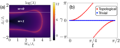
Figure 1: (a) The phase diagram of the post-quench Hamiltonian $H=H_{0}+H_{U}$.The white dashed line denotes $J_{0}=1.1$. (b) The time-dependent Berry phase in the clean limit. The blue dots are for the trivial post-quench state ($J_{0}/J_{1}=1.1$). The red dots are for the topological post-quench state with a Berry phase flow from $t=0$ to $\pi/2$ ($J_{0}/J_{1}=0.5$).

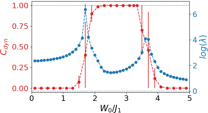
Figure 2: The disorder-average dynamical Chern number and the localization length for the post-quench Hamiltonian. The error bar is the standard deviation. There are more than $20$ disorder realizations for each data point. The parameters are $J_{0}/J_{1}=1.1,N_{x}=400$.

III.3 Entanglement spectrum

The entanglement spectrum provides the additional information of the topology induced by disorder in quench dynamics. It is shown that the crossings in the entanglement spectrum reveal the topological properties in both the equilibrium systems Li and Haldane (2008); Pollmann et al. (2010); Fidkowski (2010); Turner et al. (2010); Peschel and Chung (2011); Hughes et al. (2011); Chang et al. (2014) and out-of-equilibrium systems Gong and Ueda (2018); Chang (2018); McGinley and Cooper (2018); Pastori et al. (2020). The presence/absence of the robust crossings in the entanglement spectrum indicates the post-quench state is topological/trivial. To compute the entanglement properties, the system is bipartite spatially into $A$ and $B$ subsystems, where the post-quench many-body state is expressed as $|\Psi(t)\rangle=\sum_{i,j}C_{ij}(t)|A_{i}\rangle|B_{j}\rangle$ with $|A(B)_{i}\rangle$ being the local basis in subsystem $A(B)$. We can compute the reduced density matrix $\rho_{A}(t)={\rm Tr}_{B}|\Psi(t)\rangle\langle\Psi(t)|=\frac{1}{N}e^{-H_{A}(t)}$, where $H_{A}(t)$ is referred to the entanglement Hamiltonian, $N$ is the normalization constant, and the spectrum of $H_{A}(t)$ is the entanglement spectrum.

In free-fermion systems, the eigenvalues of the reduced density matrix can be obtained from the correlation matrix $C_{\bf x,x^{\prime}}(t)=\langle\Psi(t)|c^{\dagger}_{\bf x}c_{\bf x^{\prime}}|\Psi(t)\rangle=\sum_{i}|\psi_{i}({\bf x^{\prime}},t)\rangle\langle\psi_{i}({\bf x},t)|$, where $|\psi_{i}({\bf x},t)\rangle$ is the postquench single-particle state [see App. D]. The spectrum $\xi(t)$ of the correlation matrix $C_{\bf x,x^{\prime}}(t)$ with $x,x^{\prime}$ being restricted in $A$ is related to the entanglement spectrum $\epsilon(t)$ by $\xi(t)=1/(1+e^{\epsilon(t)})$ Peschel (2003). For simplicity, we refer $\xi(t)$ to the entanglement spectrum.

In the clean limit at $J_{0}/J_{1}=1.1$ [Fig. 3(a)], the post-quench state is trivial and no crossings in the entanglement spectrum $\xi(t)$. When the disorder strength is above the critical values, the entanglement spectrum $\xi(t)$ of the post-quench state shows a crossing at $t=\pi/4$ [Fig. 3(b)]. The existence of the crossings in the entanglement spectrum agrees with the non-vanishing dynamical Chern number of the post-quench state. We demonstrate the non-vanishing dynamical Chern number and the crossings in the entanglement spectrum for other parameters in App. E.

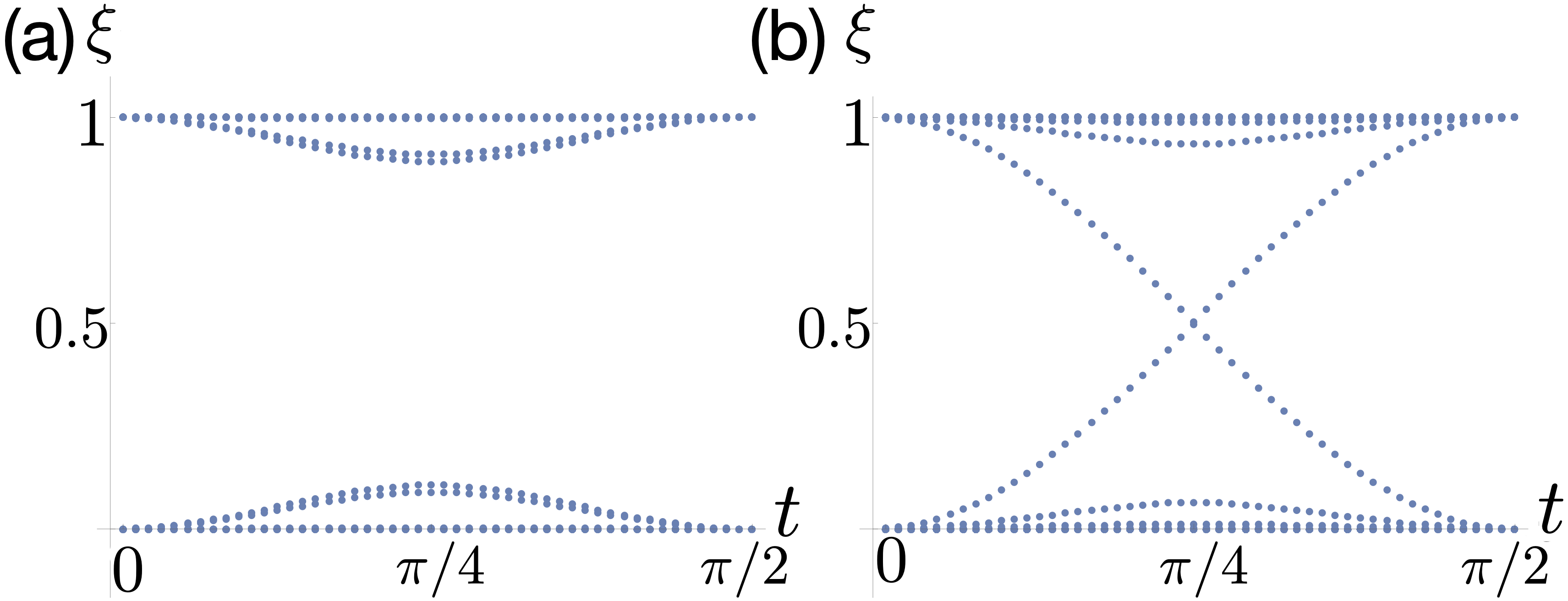
Figure 3: The entanglement spectrum of the postquench state with the bipartition $l_{A}=l_{B}=N_{x}/2$, where $l_{A(B)}$ is the length of the subsystem $A(B)$ and $N_{x}$ is the length of the total system. The parameters are $J_{0}/J_{1}=1.1$. (a) $W_{0}=0$ (clean limit). (b) $W_{0}=3$. There are $100$ disorder realizations for each data point.

IV Experimental realization

Discrete-time quantum walks are great platforms for simulating the topological phases of matter Kitagawa et al. (2010b); Cardano et al. (2017); Wang et al. (2018), quantum quenches Wang et al. (2019b); Xu et al. (2019), and disorder phenomena Obuse and Kawakami (2011); Zeng and Yong (2017); Kumar et al. (2018). Following Ref. Wang et al. (2019b), the discrete-time evolution operator for a one-dimensional lattice with single photons can be engineered by the cascaded half-wave plates and beam displacers. The Hilbert space is spanned by the polarization states $\{|P_{+}\rangle,|P_{-}\rangle\}$ and the position state $|x\rangle$ with $x\in\mathbb{Z}$. The corresponding evolution operator for each time step is $U=R(\phi_{1}/2)SR(\phi_{2})SR(\phi_{1}/2)$, where $R(\phi)$ rotate the polarization by $\phi$ with respect to $y$-axis, and $S$ is the shift operator $S=\sum_{x}|x-1\rangle\langle x|\otimes|P_{+}\rangle\langle P_{+}|+|x+1\rangle\langle x|\otimes|P_{-}\rangle\langle P_{-}|$. The polarization angle $\phi_{1(2)}(x)$ is spatially dependent and disorder can be introduced by choosing different $\phi_{1(2)}(x)$ for different position $x$.

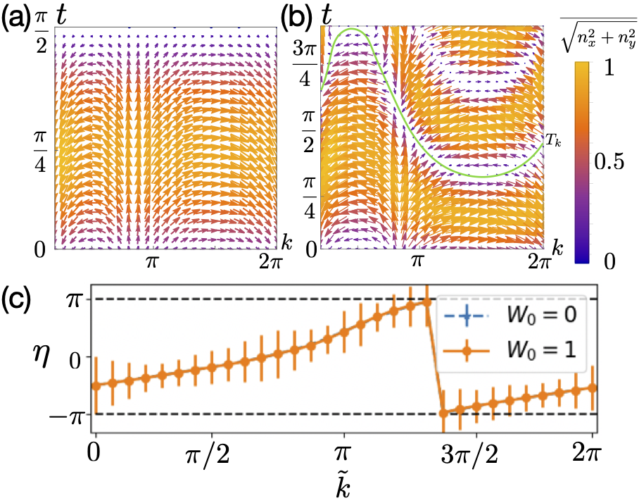
Figure 4: The post-quench psuedospin texture in the momentum-time space without disorder with $J_{0}/J_{1}=0.5$ for (a)flattened Hamiltonian, (b) non-flattened Hamiltonian. The post-quench psuedospin forms the Skyrmion texture in the momentum-time domain, $k\in[0,2\pi]$, $t\in[0,\pi/2]$ in (a) and $t\in[0,T_{k}]$ in (b) where $T_{k}=\pi/(2E(k))$ is shown by the green line. (c) The long-time average of $\eta$ for the non-flattened Hamiltonian with $J_{0}/J_{1}=0.5$. Two curves almost overlap. The error bars are the standard deviation for $400$ disorder realization. $N_{x}=31$.

In a translation-invariant case, the unitary operator can be diagonalized in the momentum space and the effective Hamiltonian describing the pre/post-quench system has the form $\mathcal{H}_{\rm eff}(k)=-i\ln U(k)$. It is shown that this quantum walk protocol Wang et al. (2019b) can simulate a sudden quench between $\mathcal{H}^{\rm i}_{\rm eff}(k)$ and $\mathcal{H}^{\rm f}_{\rm eff}(k)$ of the SSH model. Here $\mathcal{H}^{\rm i}_{\rm eff}(k)$ and $\mathcal{H}^{\rm f}_{\rm eff}(k)$ are referred to the pre-quench and the post-quench Hamiltonians. The topology of the post-quench state can be extrapolated from the post-quench pseudospin ${\bf n}(k,t)={\rm Tr}[\rho(k,t)\bm{\sigma}]$ with $\rho(k,t)=|\psi_{k}(t)\rangle\langle\psi_{k}(t)|$. The post-quench pseudospin forms the Skyrmion texture in the momentum-time domain when the post-quench state has non-vanishing dynamical Chern number [Fig. 4(a)]. The Skyrmion texture can be understood as the pseudospin pointing along the $+(-)z$ direction at $t=0(\pi/2)$ and rotating clockwise as a function of $k$ on the $x-y$ plane. In the experimental setup, the Hamiltonian is non-flatten and the period of dynamics of each momentum is $T_{k}=\pi/(2E(k))$. Nevertheless, the Skyrmion texture of the pseudospin can be observed in the momentum-time domain $k\in[0,2\pi]$, $t_{k}\in[0,T_{k}]$ [Fig. 4(b)] and was measured experimentally in the quantum walk setup Wang et al. (2019b).

In the presence of disorder, the momentum is no longer a good quantum number and the momentum-dependent period is not well-defined. For the non-flattened post-quench Hamiltoinan, we propose to measure the long-time average of the pseudospins $\overline{\langle\sigma_{i}\rangle_{T}}=\frac{1}{T}\int_{0}^{T}dt\overline{\langle\sigma_{i}\rangle}$, where $\langle\sigma_{i}\rangle={\rm Tr}\left[\rho^{\prime}(\tilde{k},t)\sigma_{i}\right]$ and

$$\rho^{\prime}(\tilde{k},t)=\overline{\frac{1}{2}\sum_{i=0}^{3}\sum_{x_{1},x_{2}}e^{-i\tilde{k}(x_{1}-x_{2})}\langle\psi_{x_{1}}(t)|\sigma_{i}|\psi_{x_{2}}(t)\rangle\sigma_{i}}.$$ (3)

$\rho^{\prime}(\tilde{k},t)$ is the disorder-averaged density matrix in the pseudomomentum-time space, where $\overline{\cdots}$ denotes the disorder average. Here $\tilde{k}$ is referred to the pseudomomentum, which indicates that the momentum is no longer a good quantum number in disordered systems. Since the $x,y-$ components of the Skyrmion texture shows a $2\pi$ winding as a function of the pseudomomemtum $\tilde{k}$, one can monitor the in-plane pseudospin texture to detect the nontrivial topology by defining

$$\eta={\rm Im}\log\left[\overline{\langle\sigma_{x}\rangle}_{T}+i\overline{\langle\sigma_{y}\rangle}_{T}\right].$$ (4)

If the the post-quench state is topological, $\eta$ shows a $2\pi$ difference in $\tilde{k}=0$ to $2\pi$.

We numerically show that $\eta$ can detect the topology of the post-quench state in Fig. 4 (c) and 5. The time taken for the average is $T=\pi/E_{min}$, where $E_{min}$ is the minimum absolute eigenenergy of the post-quench Hamiltonian in the clean limit. This average time $T$ is the largest time-scale in the system. First, we demonstrate the topology of post-quench state is robust in the weak disorder region. As shown in Fig. 4 (c), the in-plane pseudospin angle $\eta$ exhibits a $2\pi$ winding in the clean limit $W_{0}/J_{1}=0$ and the weak disorder region $W_{0}/J_{1}=1$ for the parameter $J_{0}/J_{1}=0.5$. Next, we consider the disorder-induced topology for the parameter $J_{0}/J_{1}=1.1$. As we demonstrate previously, the post-quench state is topological for the disorder strength $1.7\lesssim W_{0}/J_{1}\lesssim 3.6$. As shown in Fig. 5 (a), $\eta$ does not has a $2\pi$ winding at $W_{0}/J_{1}=1$ and $W_{0}/J_{1}=6$, but exhibits a $2\pi$ winding at $W_{0}/J_{1}=3$, reflecting the disorder-induced topology. In contrast, for the parameter $J_{0}/J_{1}=1.5$ which does not exhibit the disorder-induced topology, $\eta$ does not show a $2\pi$ winding with different strong disorder strengths as shown in Fig. 5 (b).

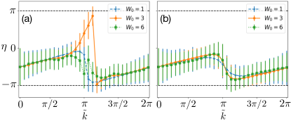
Figure 5: The long-time avarage of $\eta$ for the post-quench psuedospin in the pseudomomentum space given by non-flattened Hamiltonian with (a) $\frac{J_{0}}{J_{1}}=1.1$, and (b) $\frac{J_{0}}{J_{1}}=1.5$. The error bars are the standard deviations for $400$ disorder realizations. $N_{x}=31$.

V Conclusion

We predict the disorder-induced topology in quench dynamics in (1+1) dimensions. The topology is characterized by the dynamical Chern number and crossings in the entanglement spectrum. We show the boundaries between trivial and nontrivial post-quench states are identified by delocalized critical points in the post-quench Hamiltonian. The quantized dynamical Chern number in $(1+1)$ dimensions corresponds to the winding number of the one-dimensional topological Anderson insulating phase of the SSH model. Finally, we propose this phenomenon can be realized in quantum walk experiments.

Appendix A Localization length

When electrons are localized, the wave function exponentially decays with length, i.e. $\phi_{L}\propto e^{-L/\lambda}$, where $\phi_{L}=\sum_{n=1}^{L}(\phi_{na},\phi_{nb})^{T}c_{n}^{\dagger}$ is the eigenstate of the Hamiltonian $H=H_{o}+H_{U}$ with length $n$, $\phi_{na/b}$ are the coefficients for sublattice $a/b$ at site $n$ and $\lambda$ is the localization length. The Schrodinger equation for zero eigenenergy state becomes

$$(J_{0}+U_{1n})\phi_{nb}+(J_{1}+U_{2n})\phi_{n-1,b}=0,$$ (5)

$$(J_{0}+U_{1n})\phi_{na}+(J_{1}+U_{2n})\phi_{n+1,a}=0.$$ (6)

The above equations give the ratio of coefficients between the first and the last site, $\big{|}\phi_{La}\big{|}=\prod_{n=1}^{L}\big{|}\frac{J_{1}+U_{2n}}{J_{0}+U_{1n}}\phi_{1a}\big{|}$ and $\big{|}\phi_{Lb}\big{|}=\prod_{n=1}^{L}\big{|}\frac{J_{0}+U_{1n}}{J_{1}+U_{2n}}\phi_{1b}\big{|}$ for each sublattice, respectively. The final localization length for the system is the minimum of that of the sublattices. Thus, the localization length is given by

$$\frac{1}{\lambda}=\frac{1}{L}\ln\prod_{n=1}^{L}\big{|}\frac{J_{1}+U_{2n}}{J_{0}+U_{1n}}\big{|}.$$ (7)

The equation can be solved analytically Mondragon-Shem et al. (2014).

Another approach to calculate the localization length is via Green’s function. The localization length $\lambda$ is defined by

$$\frac{2}{\lambda}=-\lim_{L\rightarrow\infty}\frac{1}{L}\mathrm{Tr}\ln|G_{1,L}|^{2},$$ (8)

where $n$ is the total number of sites of the one-dimensional Hamiltonian, $G_{1,L}$ is the propagator connecting the first and the last slice of the system MacKinnon and Kramer (1983). $G_{1,n}$ is computed with the iterative Green’s function method MacKinnon and Kramer (1983); Kramer and MacKinnon (1993); Lewenkopf and Mucciolo (2013) by computing the onsite Green’s function $G_{n,n}=\left(E-h_{n}-U_{f}G_{n-1,n-1}U_{b}\right)$ and $G_{1,n}=G_{1,n-1}U_{b}G_{n,n}$ recursively till $n$ is large enough for convergence, where $h_{n}=(J_{0}+U_{1,n})\sigma_{x}$, $U_{f(b)}=(J_{1}+U_{2n})(\sigma_{x}+(-)i\sigma_{y})/2$ and $U_{1(2)n}$ are defined in the main text. Within this method, the Hamiltonian is constructed in a slicing scheme, i.e.

$$H_{N}=\sum_{i=1}^{N}\left(|i\rangle h_{i}\langle i|+|i\rangle U_{b}\langle i+1|+|i+1\rangle U_{f}\langle i|\right)$$ (9)

for the system with $N$ slices, where $|i\rangle$ is the state for the $i$-th slice, $U_{f(b)}$ is the forward (backward) hopping matrices between the neighboring slices, and

To calculate the Greens function for the system with $N+1$ slices, the Hamiltonian for $N+1$ slices is

$$H_{N+1}=H_{N}+|N+1\rangle h_{N+1}\langle N+1|+H^{\prime},$$ (10)

where $h_{N+1}$ is the Hamiltonian for $N+1$-th slices, the hopping matrix $H^{\prime}=|N\rangle U_{b}\langle N+1|+|N+1\rangle U_{f}\langle N|$ between the $N-$th and $N+1-$th slice is treated as a perturbing term to $H_{N}+|N+1\rangle h_{N+1}\langle N+1|$. According to Dyson equation, the perturbed Greens function is given by $G_{N+1}=G_{o}+G_{o}H^{\prime}G_{N+1}$, where $G_{o}=G_{N}+|N+1\rangle\left(E-h_{N+1}\right)^{-1}\langle N+1|$. Substitute $H^{\prime}$ into the Dyson equation, one obtains the Greens function for $N+1$ slices ($G_{N+1}$) in which the submatrices are given by

$$\langle N+1|G_{N+1}|N+1\rangle =\left(E-h_{N+1}-U_{f}\langle N|G_{N}|N\rangle U_{b}\right)^{-1},$$ (11)

$$\langle 1|G_{N+1}|N+1\rangle =\langle 1|G_{N}|N\rangle U_{b}\langle N+1|G_{N+1}|N+1\rangle.$$ (12)

Eqs. (11) and (12) are the main iterative equations for obtaining the localization length shown in Fig. 8(a).

Appendix B Symmetry analysis and topological classification

The flattened Hamiltonian formalism allows us to construct the effective Hamiltonian,

$$\mathcal{H}_{\rm eff}(k,t)=e^{-i\mathcal{H}^{F}_{0}t}\mathcal{H}_{\rm pre}(k)e^{i\mathcal{H}^{F}_{0}t}.$$ (13)

The topological invariants can be classified according to the symmetries of the effective Hamiltonian. For the pre-quench Hamiltonian $\mathcal{H}_{\rm pre}(k)=-\sigma_{z}$ and the post-quench Hamiltonian $\mathcal{H}_{0}(k)=h_{x}(k)\sigma_{x}+h_{y}(k)\sigma_{y}$, one has the effective Hamiltonian

$$\mathcal{H}_{\rm eff}(k,t) = \frac{h_{y}(k)\sin 2t}{\sqrt{h_{x}(k)^{2}+h_{y}(k)^{2}}}\sigma_{x}$$ (14)

$$-\frac{h_{x}(k)\sin 2t}{\sqrt{h_{x}(k)^{2}+h_{y}(k)^{2}}}\sigma_{y}+\cos 2t\sigma_{z}.$$

The effective Hamiltonian breaks the particle-hole symmetry explicitly, but preserves the time-reversal symmetry $\mathcal{TH}_{\rm eff}(k,t)\mathcal{T}^{-1}=\mathcal{H}_{\rm eff}(-k,-t)$, and the additional two two-fold symmetries $\sigma_{z}\mathcal{H}_{\rm eff}(k,t)\sigma_{z}=\mathcal{H}_{\rm eff}(k,-t)$, $\sigma_{x}\mathcal{H}_{\rm eff}(k,t)\sigma_{x}=-\mathcal{H}_{\rm eff}(-k,t)$. These two additional symmetries together with the time-reversal symmetry lead to a $\mathbb{Z}$ classification in $(1+1)$ dimensions. The former two-fold symmetry acts like the reflection symmetry in the time domain. There are two fixed points $t=0$ and $\pi/2$ such that $[\sigma_{z},\mathcal{H}_{\rm eff}(k,0)]=[\sigma_{z},\mathcal{H}_{\rm eff}(k,\pi/2)]=0$. The dynamical Chern number in this effective Hamiltonian is quantized in the half of the momentum-time space $k\in[0,2\pi]$, $t\in[0,\pi/2]$ Chiu et al. (2013, 2016); Morimoto and Furusaki (2013); Shiozaki and Sato (2014).

The effective Hamiltonian has the following symmetries

$$\mathcal{TH}_{\rm eff}(k,t)\mathcal{T}^{-1}=\mathcal{H}_{\rm eff}(-k,-t),$$

$$\mathcal{R}_{t}{H}_{\rm eff}(k,t)\mathcal{R}^{-1}_{t}=\mathcal{H}_{\rm eff}(k,-t),$$

$$\mathcal{M}_{x}\mathcal{H}_{\rm eff}(k,t)\mathcal{M}_{x}^{-1}=-\mathcal{H}_{\rm eff}(-k,t),$$ (15)

where $\mathcal{T}^{2}=\mathcal{R}_{t}^{2}=\mathcal{M}_{x}^{2}=1$, $\{\mathcal{R}_{t},\mathcal{M}_{x}\}=0$, and $[\mathcal{T},\mathcal{R}_{t}]=[\mathcal{T},\mathcal{M}_{x}]=0$.

The effective Hamiltonian can be expressed in terms of the effective massive Dirac Hamiltonian $\mathcal{H}_{\rm eff}(k,t)=k\gamma_{1}+t\gamma_{2}+M_{0}\gamma_{0}$, with $\{\gamma_{i},\gamma_{j}\}=0$ ($i=0,1,2$). We construct the minimal effective Dirac Hamiltonian in terms of the tensor product form of the Pauli matrices

$$\gamma_{1}=\sigma_{x}\otimes\sigma_{x},\quad\gamma_{2}=\sigma_{y}\otimes\mathbb{I}_{2\times 2},\quad\gamma_{0}=\sigma_{z}\otimes\mathbb{I}_{2\times 2},$$

$$\mathcal{T}=\mathbb{I}_{2\times 2}\otimes\sigma_{z}\mathcal{K},\quad\mathcal{R}_{t}=\sigma_{z}\otimes\sigma_{z},\quad\mathcal{M}_{x}=\sigma_{x}\otimes\mathbb{I}_{2\times 2}.$$ (16)

One can check the only allowed mass term which preserving all the symmetries is the $\gamma_{0}$. For the $\mathbb{Z}$ classification, we need to make copies of the original effective Hamiltonian. For simplicity, we just make one copy. The double Hamiltonian is $\mathcal{H}_{\rm eff}(k,t)=k\gamma_{1}\otimes\mathbb{I}_{2\times 2}+t\gamma_{2}\otimes\mathbb{I}_{2\times 2}+M_{0}\gamma_{0}\otimes\mathbb{I}_{2\times 2}$, for which there are no other symmetry-preserving mass terms. This indicates that different phases are not adiabatically connected in this system. On the other hand, we can flip one momentum of the copy and construct the double Hamiltonian, $\mathcal{H}_{\rm eff}(k,t)=k\gamma_{1}\otimes\sigma_{z}+t\gamma_{2}\otimes\mathbb{I}_{2\times 2}+M_{0}\gamma_{0}\otimes\mathbb{I}_{2\times 2}$. There is another symmetry allowed mass term (anti-commute with $\gamma_{0}\otimes\mathbb{I}_{2\times 2}\otimes\mathbb{I}_{2\times 2}$), $M_{1}=\sigma_{y}\otimes\sigma_{y}\otimes\sigma_{y}$. This indicates the systems are all in the same phase. We conclude from the above analysis that the system belongs to a $\mathbb{Z}$ classification. Similar classification schemes can be found in Refs. [Chiu et al., 2013, 2016; Morimoto and Furusaki, 2013; Shiozaki and Sato, 2014].

Appendix C Wannier center with disorders

In translational invariant systems, the Wannier orbits are constructed from the Bloch states $u_{n{\bf k}}({\bf r})$, $w_{n}({\bf r-R})=\frac{1}{\Omega}\int d{\bf k}e^{i{\bf k\cdot(r-R)}}u_{n{\bf k}}({\bf r})$, with $\Omega$ being the volume of the system, $\bf R$ is the position of the unit-cell, and $\bf r$ is the local position of the Wannier orbits within the unit-cell. In an insulator, these Wannier orbits are localized states and are the eigenstates of the projected position operator $X_{P}=PXP$, where $P$ is the projector to the occupied states which are well defined in an insulator.

To construct the Wannier orbits without using Bloch states, we first write down the Hamiltonian in the real space $\mathcal{H}_{IJ}$, where $I(J)$ includes the band indices and positions. The spectrum can exhibit a gap and the corresponding occupied states $|\psi_{\alpha I}\rangle$ are well defined. Here $\alpha$ is the eigen-energy index. The corresponding projectors are $P_{IJ}=\sum_{\alpha\in{\rm occ.}}|\psi_{\alpha I}\rangle\langle\psi_{\alpha J}|$. The position operator can be defined by as a diagonal matrix ${\rm diag}(1,\cdots,1,2,\cdots 2,\cdots,N,\cdots,N)$, where $N$ is the total number of sites and at each site there are $L$ bands. The projected position operator can be constructed as usual $X_{P}=PXP$ Kivelson (1982).

Since the Wannier orbits are the eigenstates of the $X_{P}$, we can find diagonalize the $X_{P}$ and get the set of eigenstates. If the set of the eigenstates are localized states, then these states are the Wannier orbits and the corresponding eigenvalues are the position of the Wannier states. The Wannier center of a localized state in $M$-th site can be defined as $wc_{M}=|\langle w_{M}|X_{P}|w_{M}\rangle-M|$. We have $0<\langle x_{M}\rangle<1$. We can further define the average Wannier center $\overline{wc}=\frac{1}{N}\sum_{m=1}^{N}wc_{M}$. In the presence of the chiral symmetry in one dimension gapped systems, the average Wannier center can have two values $\overline{wc}=0$ and $0.5$. The former corresponds to a trivial phase and the latter is the topological phase. Although in the quench setup, the effective Hamiltonian does not have the chiral symmetry, we observe the Wannier center of the topological post-quench state reaches $\overline{wc}=0.5$ [Fig. 6(b)]. On the other hand, for the trivial post-quench state, the Wannier center is below $0.5$ [Fig. 6(a)].

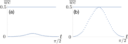
Figure 6: The Wannier center as a function of $t$. (a) Disorder-free Hamiltonian $(\frac{J_{0}}{J_{1}},\frac{W_{0}}{J_{1}})=(1.1,0)$, (b) disordered Hamiltonian $(\frac{J_{0}}{J_{1}},\frac{W_{0}}{J_{1}})=(1.1,3)$. There are $100$ disorder realizations.

Appendix D Correlation function formalism in quench setups

We consider an initial state contains $N$ particles. Each single-particle state we denote by $|\phi_{\alpha}({\bf x})\rangle,\alpha=1,\cdots,N$, ${\bf x}$ is the internal degrees of freedom, including position, spin, and the band. We require these single-particle states are orthonormal, $\sum_{\bf x}\langle\phi_{\alpha}({\bf x})|\phi_{\beta}({\bf x})\rangle=\delta_{\alpha,\beta}$. The N-particle initial state can be expressed as the Slater determinant of these single-particle state,

$$|\Psi_{0}\rangle={\rm Det}[|\phi_{i}({\bf x}_{j})\rangle],\quad i,j=1,\cdots,N.$$ (17)

We consider an unitary evolution of this initial state $|\Psi_{0}\rangle$ by a static Hamiltonian $H=\sum_{\bf x,x^{\prime}}\mathcal{H}_{\bf x,x^{\prime}}c^{\dagger}_{\bf x}c_{\bf x^{\prime}}$, where $c^{(\dagger)}_{\bf x}$ is the annihilation (creation) operator. Each single-particle state under this evolution is $|\phi_{\alpha}({\bf x},t)\rangle=\sum_{\bf x^{\prime}}\exp[-i\mathcal{H}_{\bf x,x^{\prime}}t]|\phi_{\alpha}({\bf x}^{\prime})\rangle,\alpha=1,\cdots,N$. The post-quench N-particle state is

$$|\Psi(t)\rangle=e^{-iHt}|\Psi_{0}\rangle={\rm Det}[|\phi_{i}({\bf x}_{j},t)\rangle]=\prod_{i}d_{i}^{\dagger}(t)|0\rangle,$$ (18)

where

$$d_{i}^{\dagger}(t) =e^{-iHt}d_{i}^{\dagger}e^{iHt}=e^{-iHt}\sum_{\bf y}V_{i{\bf y}}c^{\dagger}_{\bf y}e^{iHt}$$

$$=\sum_{\bf x,y}V_{i{\bf y}}U_{\bf y,x}(t)c^{\dagger}_{\bf x}$$ (19)

with $U_{\bf y,x}(t)=e^{-i\mathcal{H}_{\bf y,x}t}$ and $V_{i{\bf y}}$ being an unitary matrix that rotates $d_{i}^{\dagger}$ to $c_{\bf y}^{\dagger}$.

The post-quench single-particle state is

$$d_{i}^{\dagger}(t)|0\rangle=\sum_{\bf x,y}V_{i{\bf y}}U_{\bf y,x}(t)c^{\dagger}_{\bf x}|0\rangle=\sum_{\bf x}|\phi_{i}({\bf x},t)\rangle.$$ (20)

The correlation function constructed from the N-particle post-quench state is

$$C_{\bf x,x^{\prime}}(t) =\langle\Psi(t)|c^{\dagger}_{\bf x}c_{\bf x^{\prime}}|\Psi(t)\rangle=\langle 0|\prod_{\alpha}d_{\alpha}e^{iHt}c^{\dagger}_{\bf x}c_{\bf x^{\prime}}e^{-iHt}\prod_{\beta}d^{\dagger}_{\beta}|0\rangle\rangle$$

$$=\langle 0|\prod_{\alpha}d_{\alpha}[\sum_{{\bf y},i}d_{i}U_{\bf x,y}(t)V_{{\bf y}i}]^{\dagger}[\sum_{{\bf y^{\prime}},j}U_{\bf x^{\prime},y^{\prime}}(t)V_{{\bf y^{\prime}}j}d_{i}]\prod_{\beta}d^{\dagger}_{\beta}||0\rangle$$

$$=\sum_{i}[\sum_{\bf y}U_{\bf x,y}(t)V_{{\bf y}i}]^{\dagger}[\sum_{\bf y^{\prime}}U_{\bf x^{\prime},y^{\prime}}(t)V_{{\bf y^{\prime}}i}]$$

$$=\sum_{i}|\phi_{i}({\bf x^{\prime}},t)\rangle\langle\phi_{i}({\bf x},t)|.$$ (21)

The correlation matrix can be used for computing the entanglement spectrum. The existence of the crossings in the entanglement spectrum can detect the topology of the post-quench state as demonstrated in several examples.

Appendix E Other parameters for the disorder-induced topology in quench dynamics

In the clean limit, the dynamical Chern numbers are calculated for $0\leq J_{0}\leq 2$ and $J_{1}=1$ of the SSH Hamiltonian $H_{o}$. The results are shown in Fig. 7. For $J_{0}>1$, the static Hamiltonian becomes trivial and the dynamical Chern number is zero.

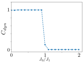
Figure 7: The dynamical Chern number (DCN) for the static Hamiltonian in the clean limit. The parameters are $J_{0}=1.1,J_{1}=1,N_{x}=400,L=20$. Here $L$ is the number of mesh points for the twisted boundary condition.

We consider the case with vanishing intercell disorder $W_{2}=0$. We find for $2.2\lesssim W_{1}\lesssim 3.8$, the dynamical Chern number is close to an integer with vanishing fluctuations as shown in Fig. 8(a). The phase boundaries, where the dynamical Chern number is close to half-integer, are at $W_{0}=1.5,4.9$. The localization length $\lambda$ also indicates delocalized transitions at the same values of $W_{0}$ [Fig. 8 (a)]. The entanglement spectrum has a crossing at $t=\pi/4$ when the post-quench state has integer dynamical Chern number $W_{1}=3$ [Fig. 8(b)].

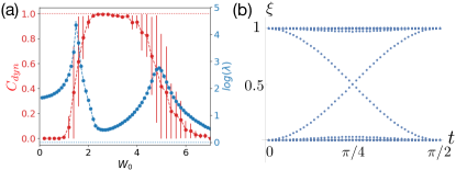
Figure 8: (color online) (a) The disorder averaged mean dynamical Chern number and localization length obtained from Eq. (8) for the quench Hamiltonian. The error bar is the standard deviation. The parameters are $J_{0}=1.1,J_{1}=1,N_{x}=100,L=400$. (b) The entanglement spectrum of the post-quench state with $W_{1}=3$. The parameters are $J_{0}=1.1,J_{1}=1,N_{x}=400$. There are more than $50$ disorder realizations for each data point.

References

- Foster et al. (2014) Matthew S. Foster, Victor Gurarie, Maxim Dzero, and Emil A. Yuzbashyan, “Quench-induced floquet topological -wave superfluids,” Phys. Rev. Lett. 113, 076403 (2014).
- Plekhanov et al. (2017) Kirill Plekhanov, Guillaume Roux, and Karyn Le Hur, “Floquet engineering of haldane chern insulators and chiral bosonic phase transitions,” Phys. Rev. B 95, 045102 (2017).
- Cooper et al. (2019) N. R. Cooper, J. Dalibard, and I. B. Spielman, “Topological bands for ultracold atoms,” Rev. Mod. Phys. 91, 015005 (2019).
- Salerno et al. (2019) G. Salerno, H. M. Price, M. Lebrat, S. Häusler, T. Esslinger, L. Corman, J.-P. Brantut, and N. Goldman, “Quantized hall conductance of a single atomic wire: A proposal based on synthetic dimensions,” Phys. Rev. X 9, 041001 (2019).
- Rechtsman et al. (2013) Mikael C. Rechtsman, Julia M. Zeuner, Yonatan Plotnik, Yaakov Lumer, Daniel Podolsky, Felix Dreisow, Stefan Nolte, Mordechai Segev, and Alexander Szameit, “Photonic floquet topological insulators,” Nature 496, 196–200 (2013).
- Wang et al. (2019a) Kunkun Wang, Xingze Qiu, Lei Xiao, Xiang Zhan, Zhihao Bian, Wei Yi, and Peng Xue, “Simulating dynamic quantum phase transitions in photonic quantum walks,” Phys. Rev. Lett. 122, 020501 (2019a).
- Ozawa et al. (2019) Tomoki Ozawa, Hannah M. Price, Alberto Amo, Nathan Goldman, Mohammad Hafezi, Ling Lu, Mikael C. Rechtsman, David Schuster, Jonathan Simon, Oded Zilberberg, and Iacopo Carusotto, “Topological photonics,” Rev. Mod. Phys. 91, 015006 (2019).
- Kyriienko and Sørensen (2018) Oleksandr Kyriienko and Anders S. Sørensen, “Floquet quantum simulation with superconducting qubits,” Phys. Rev. Applied 9, 064029 (2018).
- Malz and Smith (2021) Daniel Malz and Adam Smith, “Topological two-dimensional floquet lattice on a single superconducting qubit,” Phys. Rev. Lett. 126, 163602 (2021).
- Kitagawa et al. (2011) Takuya Kitagawa, Takashi Oka, Arne Brataas, Liang Fu, and Eugene Demler, “Transport properties of nonequilibrium systems under the application of light: Photoinduced quantum hall insulators without landau levels,” Phys. Rev. B 84, 235108 (2011).
- Ezawa (2013) Motohiko Ezawa, “Photoinduced topological phase transition and a single dirac-cone state in silicene,” Phys. Rev. Lett. 110, 026603 (2013).
- Kundu et al. (2014) Arijit Kundu, H. A. Fertig, and Babak Seradjeh, “Effective theory of floquet topological transitions,” Phys. Rev. Lett. 113, 236803 (2014).
- Gulácsi and Dóra (2015) Balázs Gulácsi and Balázs Dóra, “From floquet to dicke: Quantum spin hall insulator interacting with quantum light,” Phys. Rev. Lett. 115, 160402 (2015).
- Farrell and Pereg-Barnea (2015) Aaron Farrell and T. Pereg-Barnea, “Photon-inhibited topological transport in quantum well heterostructures,” Phys. Rev. Lett. 115, 106403 (2015).
- Takasan et al. (2017) Kazuaki Takasan, Akito Daido, Norio Kawakami, and Youichi Yanase, “Laser-induced topological superconductivity in cuprate thin films,” Phys. Rev. B 95, 134508 (2017).
- Owerre (2018) S. A. Owerre, “Photoinduced topological phase transitions in topological magnon insulators,” Scientific Reports 8, 4431 (2018).
- Lubatsch and Frank (2019) Andreas Lubatsch and Regine Frank, “Evolution of floquet topological quantum states in driven semiconductors,” The European Physical Journal B 92, 215 (2019).
- Oka and Kitamura (2019) Takashi Oka and Sota Kitamura, “Floquet engineering of quantum materials,” Annual Review of Condensed Matter Physics 10, 387–408 (2019), https://doi.org/10.1146/annurev-conmatphys-031218-013423 .
- Kitagawa et al. (2010a) Takuya Kitagawa, Erez Berg, Mark Rudner, and Eugene Demler, “Topological characterization of periodically driven quantum systems,” Phys. Rev. B 82, 235114 (2010a).
- Lindner et al. (2011) Netanel H. Lindner, Gil Refael, and Victor Galitski, “Floquet topological insulator in semiconductor quantum wells,” Nature Physics 7, 490–495 (2011).
- Jiang et al. (2011) Liang Jiang, Takuya Kitagawa, Jason Alicea, A. R. Akhmerov, David Pekker, Gil Refael, J. Ignacio Cirac, Eugene Demler, Mikhail D. Lukin, and Peter Zoller, “Majorana fermions in equilibrium and in driven cold-atom quantum wires,” Phys. Rev. Lett. 106, 220402 (2011).
- Yang et al. (2018) Chao Yang, Linhu Li, and Shu Chen, “Dynamical topological invariant after a quantum quench,” Phys. Rev. B 97, 060304(R) (2018).
- Gong and Ueda (2018) Zongping Gong and Masahito Ueda, “Topological entanglement-spectrum crossing in quench dynamics,” Phys. Rev. Lett. 121, 250601 (2018).
- Chang (2018) Po-Yao Chang, “Topology and entanglement in quench dynamics,” Phys. Rev. B 97, 224304 (2018).
- Zhu et al. (2020) Bo Zhu, Yongguan Ke, Honghua Zhong, and Chaohong Lee, “Dynamic winding number for exploring band topology,” Phys. Rev. Research 2, 023043 (2020).
- Hu and Zhao (2020) Haiping Hu and Erhai Zhao, “Topological invariants for quantum quench dynamics from unitary evolution,” Phys. Rev. Lett. 124, 160402 (2020).
- Wang et al. (2019b) Kunkun Wang, Xingze Qiu, Lei Xiao, Xiang Zhan, Zhihao Bian, Barry C. Sanders, Wei Yi, and Peng Xue, “Observation of emergent momentum–time skyrmions in parity–time-symmetric non-unitary quench dynamics,” Nature Communications 10, 2293 (2019b).
- Cardano et al. (2017) Filippo Cardano, Alessio D’Errico, Alexandre Dauphin, Maria Maffei, Bruno Piccirillo, Corrado de Lisio, Giulio De Filippis, Vittorio Cataudella, Enrico Santamato, Lorenzo Marrucci, Maciej Lewenstein, and Pietro Massignan, “Detection of zak phases and topological invariants in a chiral quantum walk of twisted photons,” Nature Communications 8, 15516 (2017).
- Xu et al. (2019) Xiao-Ye Xu, Qin-Qin Wang, Si-Jing Tao, Wei-Wei Pan, Zhe Chen, Munsif Jan, Yong-Tao Zhan, Kai Sun, Jin-Shi Xu, Yong-Jian Han, Chuan-Feng Li, and Guang-Can Guo, “Experimental classification of quenched quantum walks by dynamical chern number,” Phys. Rev. Research 1, 033039 (2019).
- Flurin et al. (2017) E. Flurin, V. V. Ramasesh, S. Hacohen-Gourgy, L. S. Martin, N. Y. Yao, and I. Siddiqi, “Observing topological invariants using quantum walks in superconducting circuits,” Phys. Rev. X 7, 031023 (2017).
- Guo et al. (2019) Xue-Yi Guo, Chao Yang, Yu Zeng, Yi Peng, He-Kang Li, Hui Deng, Yi-Rong Jin, Shu Chen, Dongning Zheng, and Heng Fan, “Observation of a dynamical quantum phase transition by a superconducting qubit simulation,” Phys. Rev. Applied 11, 044080 (2019).
- Li et al. (2009) Jian Li, Rui-Lin Chu, J. K. Jain, and Shun-Qing Shen, “Topological anderson insulator,” Phys. Rev. Lett. 102, 136806 (2009).
- Jiang et al. (2009) Hua Jiang, Lei Wang, Qing-Feng Sun, and X. C. Xie, “Numerical study of the topological anderson insulator in HgTe/CdTe quantum wells,” Phys. Rev. B 80, 165316 (2009).
- Groth et al. (2009) C. W. Groth, M. Wimmer, A. R. Akhmerov, J. Tworzydło, and C. W. J. Beenakker, “Theory of the topological anderson insulator,” Phys. Rev. Lett. 103, 196805 (2009).
- Guo et al. (2010) H.-M. Guo, G. Rosenberg, G. Refael, and M. Franz, “Topological anderson insulator in three dimensions,” Phys. Rev. Lett. 105, 216601 (2010).
- Hsu and Chen (2020) Hsiu-Chuan Hsu and Tsung-Wei Chen, “Topological anderson insulating phases in the long-range su-schrieffer-heeger model,” Phys. Rev. B 102, 205425 (2020).
- Mondragon-Shem et al. (2014) Ian Mondragon-Shem, Taylor L. Hughes, Juntao Song, and Emil Prodan, “Topological criticality in the chiral-symmetric aiii class at strong disorder,” Phys. Rev. Lett. 113, 046802 (2014).
- Titum et al. (2015) Paraj Titum, Netanel H. Lindner, Mikael C. Rechtsman, and Gil Refael, “Disorder-induced floquet topological insulators,” Phys. Rev. Lett. 114, 056801 (2015).
- Titum et al. (2016) Paraj Titum, Erez Berg, Mark S. Rudner, Gil Refael, and Netanel H. Lindner, “Anomalous floquet-anderson insulator as a nonadiabatic quantized charge pump,” Phys. Rev. X 6, 021013 (2016).
- Titum et al. (2017) Paraj Titum, Netanel H. Lindner, and Gil Refael, “Disorder-induced transitions in resonantly driven floquet topological insulators,” Phys. Rev. B 96, 054207 (2017).
- Liu et al. (2020) Hui Liu, Ion Cosma Fulga, and János K. Asbóth, “Anomalous levitation and annihilation in floquet topological insulators,” Phys. Rev. Research 2, 022048(R) (2020).
- Wauters et al. (2019) Matteo M. Wauters, Angelo Russomanno, Roberta Citro, Giuseppe E. Santoro, and Lorenzo Privitera, “Localization, topology, and quantized transport in disordered floquet systems,” Phys. Rev. Lett. 123, 266601 (2019).
- Rahmani and Vishveshwara (2018) Armin Rahmani and Smitha Vishveshwara, “Interplay of anderson localization and quench dynamics,” Phys. Rev. B 97, 245116 (2018).
- Lundgren et al. (2019) Rex Lundgren, Fangli Liu, Pontus Laurell, and Gregory A. Fiete, “Momentum-space entanglement after a quench in one-dimensional disordered fermionic systems,” Phys. Rev. B 100, 241108(R) (2019).
- Meier et al. (2018) Eric J. Meier, Fangzhao Alex An, Alexandre Dauphin, Maria Maffei, Pietro Massignan, Taylor L. Hughes, and Bryce Gadway, “Observation of the topological anderson insulator in disordered atomic wires,” Science 362, 929–933 (2018).
- Niu et al. (1985) Qian Niu, D. J. Thouless, and Yong-Shi Wu, “Quantized hall conductance as a topological invariant,” Phys. Rev. B 31, 3372–3377 (1985).
- Qi et al. (2006) Xiao-Liang Qi, Yong-Shi Wu, and Shou-Cheng Zhang, “General theorem relating the bulk topological number to edge states in two-dimensional insulators,” Phys. Rev. B 74, 045125 (2006).
- Gresch et al. (2017) Dominik Gresch, Gabriel Autès, Oleg V. Yazyev, Matthias Troyer, David Vanderbilt, B. Andrei Bernevig, and Alexey A. Soluyanov, “Z2pack: Numerical implementation of hybrid wannier centers for identifying topological materials,” Phys. Rev. B 95, 075146 (2017).
- Kuno (2019) Yoshihito Kuno, “Disorder-induced chern insulator in the harper-hofstadter-hatsugai model,” Phys. Rev. B 100, 054108 (2019).
- Bonini et al. (2020) John Bonini, David Vanderbilt, and Karin M. Rabe, “Berry flux diagonalization: Application to electric polarization,” Phys. Rev. B 102, 045141 (2020).
- Li and Haldane (2008) Hui Li and F. D. M. Haldane, “Entanglement spectrum as a generalization of entanglement entropy: Identification of topological order in non-abelian fractional quantum hall effect states,” Phys. Rev. Lett. 101, 010504 (2008).
- Pollmann et al. (2010) Frank Pollmann, Ari M. Turner, Erez Berg, and Masaki Oshikawa, “Entanglement spectrum of a topological phase in one dimension,” Phys. Rev. B 81, 064439 (2010).
- Fidkowski (2010) Lukasz Fidkowski, “Entanglement spectrum of topological insulators and superconductors,” Phys. Rev. Lett. 104, 130502 (2010).
- Turner et al. (2010) Ari M. Turner, Yi Zhang, and Ashvin Vishwanath, “Entanglement and inversion symmetry in topological insulators,” Phys. Rev. B 82, 241102(R) (2010).
- Peschel and Chung (2011) Ingo Peschel and Ming-Chiang Chung, “On the relation between entanglement and subsystem hamiltonians,” EPL (Europhysics Letters) 96, 50006 (2011).
- Hughes et al. (2011) Taylor L. Hughes, Emil Prodan, and B. Andrei Bernevig, “Inversion-symmetric topological insulators,” Phys. Rev. B 83, 245132 (2011).
- Chang et al. (2014) Po-Yao Chang, Christopher Mudry, and Shinsei Ryu, “Symmetry-protected entangling boundary zero modes in crystalline topological insulators,” Journal of Statistical Mechanics: Theory and Experiment 2014, P09014 (2014).
- McGinley and Cooper (2018) Max McGinley and Nigel R. Cooper, “Topology of one-dimensional quantum systems out of equilibrium,” Phys. Rev. Lett. 121, 090401 (2018).
- Pastori et al. (2020) Lorenzo Pastori, Simone Barbarino, and Jan Carl Budich, “Signatures of topology in quantum quench dynamics and their interrelation,” Phys. Rev. Research 2, 033259 (2020).
- Peschel (2003) Ingo Peschel, “Calculation of reduced density matrices from correlation functions,” Journal of Physics A: Mathematical and General 36, L205–L208 (2003).
- Kitagawa et al. (2010b) Takuya Kitagawa, Mark S. Rudner, Erez Berg, and Eugene Demler, “Exploring topological phases with quantum walks,” Phys. Rev. A 82, 033429 (2010b).
- Wang et al. (2018) Xiaoping Wang, Lei Xiao, Xingze Qiu, Kunkun Wang, Wei Yi, and Peng Xue, “Detecting topological invariants and revealing topological phase transitions in discrete-time photonic quantum walks,” Phys. Rev. A 98, 013835 (2018).
- Obuse and Kawakami (2011) Hideaki Obuse and Norio Kawakami, “Topological phases and delocalization of quantum walks in random environments,” Phys. Rev. B 84, 195139 (2011).
- Zeng and Yong (2017) Meng Zeng and Ee Hou Yong, “Discrete-time quantum walk with phase disorder: Localization and entanglement entropy,” Scientific Reports 7, 12024 (2017).
- Kumar et al. (2018) N. Pradeep Kumar, Subhashish Banerjee, and C. M. Chandrashekar, “Enhanced non-markovian behavior in quantum walks with markovian disorder,” Scientific Reports 8, 8801 (2018).
- MacKinnon and Kramer (1983) A. MacKinnon and B. Kramer, “The scaling theory of electrons in disordered solids: Additional numerical results,” Zeitschrift für Physik B Condensed Matter 53, 1–13 (1983).
- Kramer and MacKinnon (1993) B Kramer and A MacKinnon, “Localization: theory and experiment,” Reports on Progress in Physics 56, 1469–1564 (1993).
- Lewenkopf and Mucciolo (2013) Caio H. Lewenkopf and Eduardo R. Mucciolo, “The recursive green’s function method for graphene,” Journal of Computational Electronics 12, 203–231 (2013).
- Chiu et al. (2013) Ching-Kai Chiu, Hong Yao, and Shinsei Ryu, “Classification of topological insulators and superconductors in the presence of reflection symmetry,” Phys. Rev. B 88, 075142 (2013).
- Chiu et al. (2016) Ching-Kai Chiu, Jeffrey C. Y. Teo, Andreas P. Schnyder, and Shinsei Ryu, “Classification of topological quantum matter with symmetries,” Rev. Mod. Phys. 88, 035005 (2016).
- Morimoto and Furusaki (2013) Takahiro Morimoto and Akira Furusaki, “Topological classification with additional symmetries from clifford algebras,” Phys. Rev. B 88, 125129 (2013).
- Shiozaki and Sato (2014) Ken Shiozaki and Masatoshi Sato, “Topology of crystalline insulators and superconductors,” Phys. Rev. B 90, 165114 (2014).
- Kivelson (1982) S. Kivelson, “Wannier functions in one-dimensional disordered systems: Application to fractionally charged solitons,” Phys. Rev. B 26, 4269–4277 (1982).