Abstract

In the standard framework of self-consistent many-body perturbation theory, the skeleton series for the self-energy is truncated at a finite order $N$ and plugged into the Dyson equation, which is then solved for the propagator $G_{N}$. For two simple examples of fermionic models – the Hubbard atom at half filling and its zero space-time dimensional simplified version – we find that $G_{N}$ converges when $N\to\infty$ to a limit $G_{\infty}$, which coincides with the exact physical propagator $G_{\rm exact}$ at small enough coupling, while $G_{\infty}\neq G_{\rm exact}$ at strong coupling. We also demonstrate that it is possible to discriminate between these two regimes thanks to a criterion which does not require the knowledge of $G_{\rm exact}$, as proposed in [1].

1 Introduction

Self-consistent perturbation theory is a particularly elegant and powerful approach in quantum many-body physics [2, 3]. The single-particle propagator $G$ is expressed through the Dyson equation

$$G^{-1}=G_{0}^{-1}-\Sigma$$ (1)

in terms of the non-interacting propagator $G_{0}$ and the self-energy $\Sigma$, which itself is formally expressed in terms of $G$ through the skeleton series

$$\Sigma=\Sigma_{\rm bold}[G]=\sum_{n=1}^{\infty}\Sigma_{\rm bold}^{(n)}[G]$$ (2)

where $\Sigma_{\rm bold}^{(n)}[G]$ is the sum of all two-particle irreducible Feynman diagrams of order $n$ (built with bold propagator lines representing $G$).

The standard procedure for solving Eqs. (1,2) is to truncate the skeleton series at a finite order $N$, and to look for the solution $G_{N}$ of the self-consistency equation

$$G_{N}^{-1}=G_{0}^{-1}-\Sigma_{\rm bold}^{(\leq N)}[G_{N}]$$ (3)

with $\Sigma_{\rm bold}^{(\leq N)}:=\sum_{n=1}^{N}\Sigma_{\rm bold}^{(n)}$. The natural expectation is that one obtains the exact propagator by sending the truncation order to infinity: $G_{N}\to G_{\rm exact}$ for $N\to\infty$.

However, as was discovered in [4], the series $\Sigma_{\rm bold}^{(\leq N)}[G_{\rm exact}]$ can converge when $N\to\infty$ to a result which differs from the exact physical self-energy $\Sigma_{\rm exact}=G_{0}^{-1}-G_{\rm exact}^{-1}$. This misleading convergence phenomenon was observed for three fermionic textbook models —Hubbard atom, Anderson impurity model, and half-filled 2D Hubbard model— in a region of the parameter space (at and around half filling, at strong interaction and low temperature). $G_{\rm exact}$ was computed with a numerically exact quantum Monte Carlo method, and the skeleton series was evaluated up to $N=6$ or 8 by diagrammatic Monte Carlo [5]. Numerous works [6, 7, 1, 8, 9, 10, 11, 12, 13, 14] have studied various aspects of the problem found in [4], as well as the related divergences of irreducible vertices (​​[8, 10, 11, 13, 15, 16, 17, 18] and Refs. therein). In particular, Ref. [7] introduced an exactly solvable toy model, which has the structure of a fermionic model in zero space-time dimensions, and features the misleading convergence problem of [4].

In this article, we study the consequences of this problem for the sequence $G_{N}$, which is the crucial question in the most relevant cases where $G_{\rm exact}$ is unknown. For the toy model of [7], we find that $G_{N}$ converges when $N\to\infty$ to a limit $G_{\infty}$ which differs from $G_{\rm exact}$ at strong coupling. For the Hubbard atom, our numerical data strongly indicate that such misleading convergence of the sequence $G_{N}$ also occurs at large coupling and half filling. Moreover, we demonstrate that a criterion proposed in [1] allows to discriminate between the $G_{\infty}\neq G_{\rm exact}$ and $G_{\infty}=G_{\rm exact}$ regimes without using the knowledge of $G_{\rm exact}$.

We note that although we restrict here to the scheme (1,2) where $G$ is the only bold element, our findings may also be relevant to other schemes containing additional bold elements, such as a bold interaction line $W$, or a bold pair propagator line $\Gamma$. The scheme built with $G$ and $W$ is natural for Coulomb interactions, and is widely used for solids and molecules with a truncation order $N=1$ (the $GW$ approximation) and sometimes with $N=2$ (see, e.g., Refs. [19, 20, 21, 22]), while for several paradigmatic lattice models, bold diagrammatic Monte Carlo (BDMC) made it possible to reach larger $N$ and claim a small residual trunction error [23, 24, 25, 26]. The scheme built with $G$ and $\Gamma$ is natural for contact interactions; truncation at order $N=1$ then corresponds to the self-consistent T-matrix approximation [27, 28, 29], and precise large-$N$ results were obtained by BDMC in the normal phase of the Hubbard model [30, 31] and of the unitary Fermi gas [32, 33, 34]. Other BDMC results were obtained for models of coupled electrons and phonons, where it is natural to introduce a bold phonon propagator [35, 23], and for frustrated spins [36, 37, 38]. Schemes containing three- or four-point bold vertices were also employed, to construct extensions of dynamical mean-field theory [39, 17].

2 Zero space-time dimensional toy-model

2.1 Definitions and reminders

We begin with some reminders from [7]. While fermionic many-body problems can be represented by a functional integral over Grassmann fields, which depend on $d$ space coordinates and one imaginary time coordinate [40], in this simplified toy model the Grassmann fields are replaced with Grassmann numbers $\varphi_{s}$ and $\bar{\varphi}_{s}$ that do not depend on anything, apart from a spin index ${s}\in\{\uparrow,\downarrow\}$. The partition function, the action and the propagator are then defined by

$$Z=\int\left(\prod_{{s}}d\varphi_{s}d\bar{\varphi}_{s}\right)\;e^{-S[\bar{\varphi}_{s},\varphi_{s}]}$$

$$S[\bar{\varphi}_{s},\varphi_{s}]=-\mu\sum_{s}\bar{\varphi}_{s}\varphi_{s}+U\bar{\varphi}_{\uparrow}\varphi_{\uparrow}\bar{\varphi}_{\downarrow}\varphi_{\downarrow}$$

$$G=-\frac{1}{Z}\ \int\left(\prod_{s}d\varphi_{s}d\bar{\varphi}_{s}\right)\;e^{-S[\bar{\varphi}_{s},\varphi_{s}]}\ \varphi_{s}\,\bar{\varphi}_{s},$$

the dimensionless parameters $\mu$ and $U$ being the analogs of chemical potential and interaction strength. We restrict for convenience to $\mu>0$ (changing the sign of $\mu$ essentially amounts to the change of variables $\varphi\leftrightarrow\bar{\varphi}$) and to $U<0$ (as in [7]).

The coefficients of the skeleton series have the analytical expression

$$\Sigma_{\rm bold}[G]=\sum_{n=1}^{\infty}{a_{n}}\,G^{2n-1}U^{n}\ \ \ \ \ \ {\rm with}\ \ \ \ \ \ {a_{n}}=\frac{(-1)^{n-1}(2n-2)!}{n!(n-1)!}.$$

It is convenient to work with rescaled variables, multiplying propagators with $\sqrt{|U|}$ and dividing self-energies with the same factor,

$$g\coloneqq G\sqrt{|U|},\ \ \ \ \ \ \sigma\coloneqq\Sigma/\sqrt{|U|}.$$ (4)

The rescaled skeleton series is then given by

$$\sigma_{\rm bold}(g)=\sum_{n=1}^{\infty}\sigma_{\rm bold}^{(n)}(g)\ \ \ \ \ \ {\rm with}\ \ \ \ \ \ \sigma_{\rm bold}^{(n)}(g)={a_{n}}(-1)^{n}g^{2n-1}$$

and accordingly $\sigma_{\rm bold}^{(\leq N)}(g)\equiv\sum_{n=1}^{N}\sigma_{\rm bold}^{(n)}(g)$.

The exact self-energy and propagator are given by

$$\sigma_{\rm exact}(g_{0}) = -g_{0}$$

$$g_{\rm exact}(g_{0}) = \frac{g_{0}}{1+g_{0}^{2}}$$

in terms of the rescaled free propagator $g_{0}:=\sqrt{|U|}\,G_{0}=\sqrt{|U|}/\mu$.

If one evaluates the bold series at the exact $G$, one obtains the correct physical self-energy for $|U|<\mu^{2}$ and an incorrect result for $|U|>\mu^{2}$. More precisely, the self-energy functional (which reduces to a function in this toy model) has the two branches

$$\sigma^{(\pm)}(g)=\frac{-1\pm\sqrt{1-4g^{2}}}{2g}$$ (5)

as represented on Fig. 1. The physical branch is the $(+)$ branch for $g_{0}<1$, and the $(-)$ branch for $g_{0}>1$; i.e., $\sigma_{\rm exact}(g_{0})=\sigma^{({\rm sign}(1-g_{0}))}(g_{\rm exact}(g_{0}))$. On the other hand, the bold series, evaluated at the exact physical propagator, always converges to the $(+)$ branch; i.e., $\sigma_{\rm bold}(g_{\rm exact}(g_{0}))=\sigma^{(+)}(g_{\rm exact}(g_{0}))$ for all $g_{0}>0$.

Note that $\sigma_{\rm bold}(g)$ is the expansion of $\sigma^{(+)}(g)$ in powers of $g$, and thus from (5) the convergence radius of the series $\sigma_{\rm bold}(g)$ is 1/2.

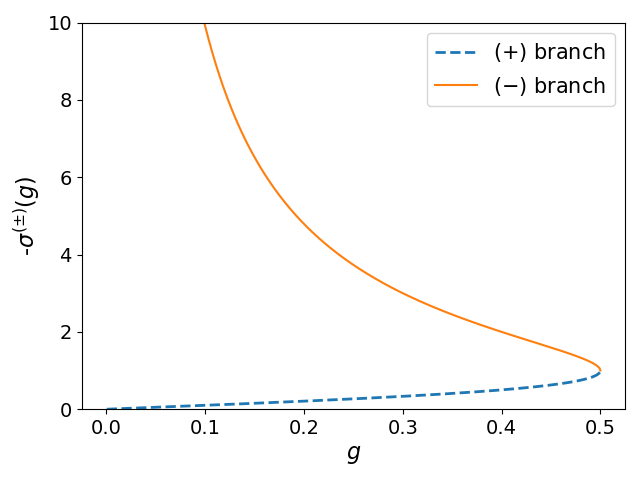
Figure 1: The two branches of the self-energy as a function of the full propagator, for the toy model in zero space-time dimensions. The skeleton series converges up to $g=1/2$ and coincides with the $(+)$ branch: $\sigma_{\rm bold}(g)=\sigma^{(+)}(g)$ for $g\leq 1/2$.

2.2 Limit of the skeleton sequence

We will refer to the sequence $G_{N}$ as the skeleton sequence. Rescaling variables as in (4), in particular setting $g_{N}\coloneqq G_{N}\sqrt{|U|}$, the self-consistency equation (3) becomes

$$\frac{1}{g_{N}}=\frac{1}{g_{0}}-\sigma_{\rm bold}^{(\leq N)}(g_{N}).$$ (6)

This equation is readily solved for $g_{N}$ numerically: The solutions are roots of a polynomial of order $2N$, and we observe that there is a unique real positive root, which we take to be $g_{N}$ (recall that the exact $g$ is always real and positive); alternatively, we solved Eq. (6) by iterations (with a damping procedure described in the next Section), and we found convergence to this same $g_{N}$. We find that

• for $g_{0}<1$,   $g_{N}\underset{N\to\infty}{\longrightarrow}g_{\rm exact}(g_{0})$

• for $g_{0}>1$,   $g_{N}\underset{N\to\infty}{\longrightarrow}g_{\infty}\neq g_{\rm exact}(g_{0})$

i.e., the skeleton sequence converges to the correct physical result below a critical coupling strength, and to an unphysical result above it.

Let us focus on the regime $g_{0}>1$, where the convergence to an unphysical result takes place (as demonstrated in Fig. 3). The fact that the skeleton sequence converges at all in this regime is non-trivial. The value of the unphysical limit $g_{\infty}=1/2$ of the skeleton sequence $g_{N}$ is equal to the radius of convergence of the skeleton series $\sigma_{\rm bold}(g)$. This is not a coincidence, and the reason for this self-tuning towards the convergence radius becomes clear from Fig. 3: For a large truncation order, the curve representing the truncated bold series as a function of $g$ becomes an almost vertical line above the position of the convergence radius ($g=1/2$), so that it intersects the Dyson-equation curve near this value of $g$. It also becomes clear that we are in an unusual situation where

$$\lim_{N\to\infty}\sigma_{\rm bold}^{(\leq N)}(g_{N})\neq\lim_{N\to\infty}\sigma_{\rm bold}^{(\leq N)}(g_{\infty})\equiv\sigma_{\rm bold}(g_{\infty}).$$

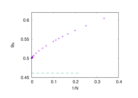
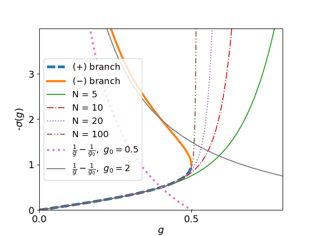
Figure 2: Illustrative example of misleading convergence of the skeleton sequence for the toy model. The rescaled propagator $g_{N}$, obtained from the self-consistency equation with the skeleton series truncated at order $N$, converges for $N\to\infty$ to the limit 0.5, which differs from the exact result (dashed line). This happens when the rescaled free propagator $g_{0}>1$ (here, $g_{0}=1.5$).

Figure 3: Explanation for the misleading convergence. The two branches of the self-energy $\sigma^{(\pm)}(g)$, together with the partial sums of the skeleton series $\sigma_{\rm bold}^{(\leq N)}(g)$ for different values of the truncation order $N$. Also shown is the curve corresponding to the Dyson equation, $-\sigma=1/g-1/g_{0}$. This Dyson-equation curve intersects $\sigma_{\rm bold}^{(\leq N)}(g)$ at $g=g_{N}$, whereas the exact propagator $g=g_{\rm exact}$ is given by the intersection of the Dyson-equation curve with the physical branch $\sigma^{({\rm sign}(1-g_{0}))}(g)$. It appears clearly that for $g_{0}<1$, $g_{N}$ converges to the exact $g$, while for $g_{0}>1$, $g_{N}$ always tends to $1/2$, the convergence radius of the skeleton series.

2.3 Diagnosing the misleading convergence

In the general case where $G_{\rm exact}$ is unknown, when one observes numerically that $G_{N}$ converges to some limit, one needs a way to tell whether or not this limit is equal to $G_{\rm exact}$. Assuming that $G_{N}\to G_{\infty}$ for $N\to\infty$, the following criterion [1] is a sufficient condition for $G_{\infty}$ to be equal to $G_{\rm exact}$:

There exists $$\epsilon>0 \xi \mathcal{D}=\{|\xi|<1+\epsilon\}$$ such that for any in the disc ,

       $$\Sigma_{N,\xi} N\to\infty$$ converges for ;

moreover, this sequence is uniformly bounded for $$\xi\in\mathcal{D}$$

where

$$\Sigma_{N,\xi}\coloneqq\sum_{n=1}^{N}\Sigma_{\rm bold}^{(n)}[G_{N}]\,\xi^{n}.$$ (7)

For all practical purpose, we expect this criterion to be essentially equivalent to the following simpler one:

$$\textrm{\it There exists {$\xi>1$} such that}\ \ \Sigma_{N,{\xi}}\ \textrm{\it converges for }N\to\infty.$$ (8)

In what follows we will use this simplified criterion. We also introduce an extra factor $1/\xi^{N_{0}}$ in the definition (7) of $\Sigma_{N,\xi}$, where the value of $N_{0}$ will be conveniently chosen; such an $N$-independent factor does not matter for the criterion (it does not change whether or not the sequence $\Sigma_{N,\xi}$ converges).

For the toy-model, this means that assuming $g_{N}\to g_{\infty}$ for $N\to\infty$, a sufficient condition for $g_{\infty}$ to be equal to the correct physical $g_{\rm exact}(g_{0})$ is that there exists $\xi>1$ such that

$$\sigma_{N,\xi}\coloneqq\sum_{n=1}^{N}\sigma_{\rm bold}^{(n)}(g_{N})\,{\xi}^{n-1}=\sigma_{\rm bold}^{(\leq N)}(g_{N}\sqrt{{\xi}})\ /\ \sqrt{{\xi}}$$ (9)

converges for $N\to\infty$. As illustrated in Fig. 4, this criterion indeed allows to detect the misleading convergence for $g_{0}>1$, and to trust the result for $g_{0}<1$.

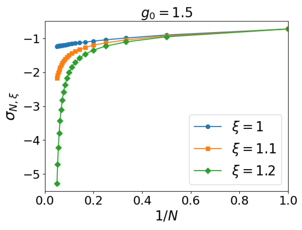
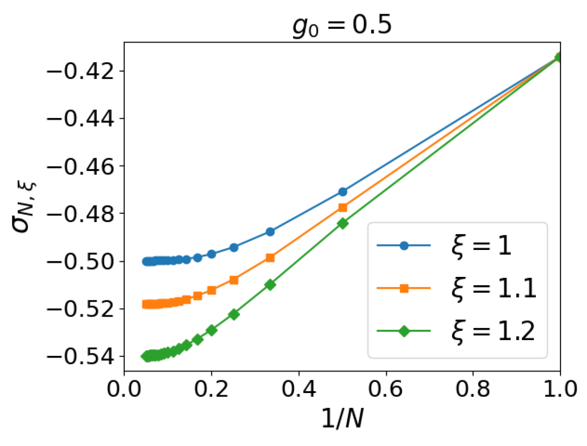
Figure 4: Detecting the misleading convergence for the toy model. Introducing a finite ${\xi}$ , the sequence becomes divergent which allows to detect the problem (left), or remains convergent which allows to trust the result (right).

3 Hubbard atom

We turn to the single-site Hubbard model, defined by the grand-canonical Hamiltonian $-\mu\sum_{s}n_{s}+Un_{\uparrow}n_{\downarrow}$. The propagator can be expressed as a functional integral over $\beta$-antiperiodic Grassmann fields [40],

$$G_{s}(\tau)=-\frac{\int\mathcal{D}\varphi\mathcal{D}\bar{\varphi}\ \ \varphi_{s}(\tau)\bar{\varphi}_{s}(0)\,e^{-S}}{\int\mathcal{D}\varphi\mathcal{D}\bar{\varphi}\,e^{-S}}$$ (10)

with the action

$$S=\int_{0}^{\beta}d\tau\ \left[-\sum_{s}\bar{\varphi}_{s}(\tau)(G_{0}^{-1}\,\varphi_{s})(\tau)+U(\bar{\varphi}_{\uparrow}\bar{\varphi}_{\downarrow}\varphi_{\downarrow}\varphi_{\uparrow})(\tau)\right]$$ (11)

and

$$G_{0}^{-1}=\mu-\frac{d}{d\tau}.$$ (12)

We restrict for simplicity to the half-filled case $\mu=U/2$, which should be the most dangerous case, since it is at and around half-filling that the misleading convergence of $\Sigma_{\rm bold}[G_{\rm exact}]$ was discovered in [4]. We use the BDMC method [41, 5, 32, 42] to sum all skeleton diagrams and solve the self-consistency equation (3) for truncation orders $N\leq 8$ (note that at half filling, $\Sigma_{\rm bold}^{(n)}=0$ for all odd $n>1$).

The first question is whether the skeleton sequence $G_{N}$ can also converge to an unphysical result, or equivalently, whether $\Sigma_{\rm bold}^{(\leq N)}[G_{N}]=:\Sigma_{N}$ can converge to an unphysical result. Let us first consider the double occupancy

$$D=\langle n_{\uparrow}n_{\downarrow}\rangle=U^{-1}\,{\rm tr}(\Sigma\,G)$$ (13)

and the corresponding sequence $D_{N}:=U^{-1}\,{\rm tr}(\Sigma_{N}\,G_{N})$. At large enough $U$, our data strongly indicate that this sequence does converge (albeit slowly) towards an unphysical result, see left panel of Fig. 5. For small enough $U$, there is a fast convergence to the correct result, see right panel of Fig. 5.

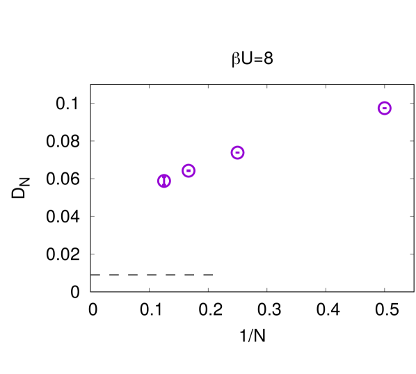
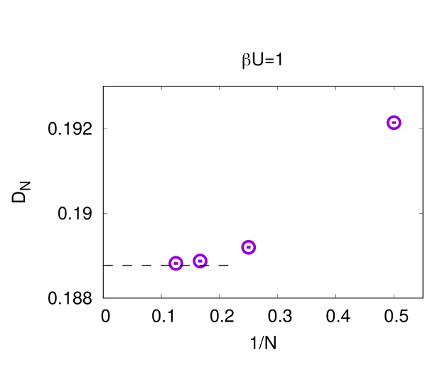
Figure 5: For the Hubbard atom at half filling, the double occupancy, as obtained from the skeleton sequence, converges to an unphysical result for large $U$ (left) and to the correct result for small enough $U$ (right) when the truncation order $N\to\infty$ (dashed line: exact result).

The next question is whether the criterion (8) allows us to discriminate between these two situations. We therefore plot the sequence $\Sigma_{N,{\xi}}$ in Figs. 7 and 7. We only show the imaginary part because in the considered half-filled case, the real part of $\Sigma_{N}(\omega_{n})$ automatically equals $U/2$; moreover we focus for simplicity on the lowest Matsubara frequency $\omega_{0}=\pi/\beta$, and we choose $N_{0}=2$.

For ${\xi=1}$, $\Sigma_{N,{\xi}}$ reduces to the original skeleton sequence $\Sigma_{N}$, and the behavior is similar to the double occupancy: The sequence appears to converge, albeit slowly, towards an unphysical result for $\beta U=8$ (Fig. 7), while fast convergence to the correct physical result takes place for $\beta U=1$ (Fig. 7). For ${\xi>1}$, the sequence does not appear to converge any more for $\beta U=8$, see Fig. 7: The criterion correctly indicates that the results should not be trusted in this case. In contrast, for $\beta U=1$, the criterion allows to validate the results, since the sequence remains convergent at ${\xi>1}$, see Fig. 7. Regarding the choice of ${\xi}$, it should be neither too small in order to have an effect at the accessible orders, nor too large to avoid making the criterion too conservative; here we see that $\xi=1.1$ and 1.2 are appropriate.

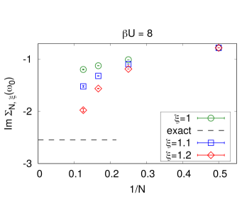
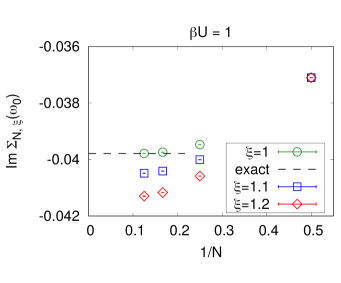
Figure 6: For the half-filled Hubbard atom at large coupling, the original skeleton sequence $(\xi=1)$ converges to an unphysical result. At ${\xi>1}$, the sequence does not converge any more: The criterion allows to detect the misleading convergence.

Figure 7: For the half-filled Hubbard atom at small enough coupling, the original skeleton sequence ($\xi=1$) converges to the correct physical result. At $\xi>1$, the sequence remains convergent: The criterion allows to trust the result.

We remark that when solving Eq. (3) by iterations, in the case where the convergence to the unphysical result for $N\to\infty$ occurs, convergence as a function of iterations at fixed $N$ only takes place if we use a damping procedure, where $G_{N}$ at iteration $(i+1)$ is obtained as $G_{N}^{(i+1)}=[G_{0}^{-1}-\Sigma^{(i)}]^{-1}$ with $\Sigma^{(i)}$ a weighted average of $\Sigma_{\rm bold}^{(\leq N)}(G_{N}^{(i)})$ and $\Sigma^{(i-1)}$ [while the fixed point is unstable for the undamped iterative procedure $\Sigma^{(i)}\coloneqq\Sigma_{\rm bold}^{(\leq N)}(G_{N}^{(i)})$ ]. Such a damping procedure is commonly used in BDMC where it also reduces the statistical error [43, 42]. In the toy model, one can easily show that an increasingly strong damping is required when $N$ is increased, because for $N\to\infty$, the slope $[d\sigma_{\rm bold}^{(\leq N)}(g)/dg]_{g=g_{N}}$ diverges, making the undamped iterative procedure unstable. This observation could also be useful for misleading-convergence detection.

Finally, we comment on the link with the multivaluedness of the self-energy functional $\Sigma[G]$ (i.e., of the Luttinger-Ward functional). In [4], the misleading convergence of the skeleton series was found to be towards an unphysical branch of the self-energy functional, in the sense that if Eqs. (10,11) are viewed as a mapping $G_{0}\mapsto G[G_{0}]$, then there exists $G_{0,{\rm unphys}}$ such that $\Sigma_{\rm bold}[G_{\rm exact}]=G_{0,{\rm unphys}}^{-1}-G_{\rm exact}^{-1}$ and $G[G_{0,{\rm unphys}}]=G_{\rm exact}\equiv G[G_{0}]$. As noted in [4], this $G_{0,{\rm unphys}}$ does not belong to the set of physical bare propagators which are of the form (12) for some value of chemical potential; therefore, by looking at $G_{0,{\rm unphys}}$, one can tell that the result is on an unphysical branch, and hence detect the misleading convergence of the skeleton series. In contrast, the misleading convergence of the skeleton sequence found here cannot be detected in this way. Indeed, the self-consistency equation (3) is enforced with the original physical $G_{0}$.

4 Conclusion

We have observed that there is a regime where the solution of self-consistent many-body perturbation theory converges to an unphysical result in the limit of infinite truncation order of the skeleton series. This surprising breakdown of the standard framework results from a subtle mathematical mechanism which we have clarified by analyzing the zero space-space dimensional model. In this problematic regime, lowest order calculations can be off by one order of magnitude, but access to higher orders allows to detect the problem numerically through the divergence of a slightly modified sequence, whereas seeing convergence of this modified sequence allows to rule out misleading convergence and to trust the result, as proposed in [1] and demonstrated here for the Hubbard atom. Such a proof of principle is relevant for many-body problems in regimes where, in spite of important progress with non self-consistent frameworks [44, 45, 46, 47, 48, 49, 50, 51, 52, 53, 54] (for which misleading convergence generically does not occur [1]), self-consistent BDMC remains the state of the art to date. In particular, the present findings served as a basis to discriminate between physical and unphysical BDMC results for the doped two-dimensional Hubbard model at strong coupling in a non-Fermi liquid regime [55].

References

- [1] R. Rossi, F. Werner, N. Prokof’ev and B. Svistunov, Shifted-Action Expansion and Applicability of Dressed Diagrammatic Schemes, Phys. Rev. B 93, 161102(R) (2016), 10.1103/PhysRevB.93.161102.
- [2] R. M. Martin, L. Reining and D. M. Ceperley, Interacting Electrons: Theory and Computational Approaches, Cambridge University Press, 10.1017/CBO9781139050807 (2016).
- [3] G. Stefanucci and R. van Leeuwen, Nonequilibrium Many-Body Theory of Quantum Systems: A Modern Introduction, Cambridge University Press, New York, 10.1017/CBO9781139023979 (2013).
- [4] E. Kozik, M. Ferrero and A. Georges, Nonexistence of the Luttinger-Ward Functional and Misleading Convergence of Skeleton Diagrammatic Series for Hubbard-Like Models, Phys. Rev. Lett. 114, 156402 (2015), 10.1103/PhysRevLett.114.156402.
- [5] K. Van Houcke, E. Kozik, N. Prokof’ev and B. Svistunov, Diagrammatic Monte Carlo, in Computer Simulation Studies in Condensed Matter Physics XXI. CSP-2008. Eds. D.P. Landau, S.P. Lewis, and H.B. Schüttler, Phys. Procedia 6, 95, 10.1016/j.phpro.2010.09.034 (2010).
- [6] A. Stan, P. Romaniello, S. Rigamonti, L. Reining and J. Berger, Unphysical and physical solutions in many-body theories: from weak to strong correlation, New J. Phys. 17, 093045 (2015).
- [7] R. Rossi and F. Werner, Skeleton series and multivaluedness of the self-energy functional in zero space-time dimensions, J. Phys. A 48, 485202 (2015), 10.1088/1751-8113/48/48/485202.
- [8] T. Schäfer, S. Ciuchi, M. Wallerberger, P. Thunström, O. Gunnarsson, G. Sangiovanni, G. Rohringer and A. Toschi, Nonperturbative landscape of the Mott-Hubbard transition: Multiple divergence lines around the critical endpoint, Phys. Rev. B 94, 235108 (2016), 10.1103/PhysRevB.94.235108.
- [9] W. Tarantino, P. Romaniello, J. A. Berger and L. Reining, Self-consistent Dyson equation and self-energy functionals: An analysis and illustration on the example of the Hubbard atom, Phys. Rev. B 96, 045124 (2017), 10.1103/PhysRevB.96.045124.
- [10] O. Gunnarsson, G. Rohringer, T. Schäfer, G. Sangiovanni and A. Toschi, Breakdown of Traditional Many-Body Theories for Correlated Electrons, Phys. Rev. Lett. 119, 056402 (2017), 10.1103/PhysRevLett.119.056402.
- [11] J. Vučičević, N. Wentzell, M. Ferrero and O. Parcollet, Practical consequences of the Luttinger-Ward functional multivaluedness for cluster DMFT methods, Phys. Rev. B 97, 125141 (2018), 10.1103/PhysRevB.97.125141.
- [12] L. Lin and M. Lindsey, Variational structure of Luttinger–Ward formalism and bold diagrammatic expansion for Euclidean lattice field theory, PNAS 115(10), 2282 (2018), 10.1073/pnas.1720782115.
- [13] P. Chalupa, P. Gunacker, T. Schäfer, K. Held and A. Toschi, Divergences of the irreducible vertex functions in correlated metallic systems: Insights from the Anderson impurity model, Phys. Rev. B 97, 245136 (2018), 10.1103/PhysRevB.97.245136.
- [14] A. J. Kim and V. Sacksteder, Multivaluedness of the Luttinger-Ward functional in the fermionic and bosonic system with replicas, Phys. Rev. B 101, 115146 (2020), 10.1103/PhysRevB.101.115146.
- [15] T. Schäfer, G. Rohringer, O. Gunnarsson, S. Ciuchi, G. Sangiovanni and A. Toschi, Divergent Precursors of the Mott-Hubbard Transition at the Two-Particle Level, Phys. Rev. Lett. 110, 246405 (2013), 10.1103/PhysRevLett.110.246405.
- [16] O. Gunnarsson, T. Schäfer, J. P. F. LeBlanc, J. Merino, G. Sangiovanni, G. Rohringer and A. Toschi, Parquet decomposition calculations of the electronic self-energy, Phys. Rev. B 93, 245102 (2016), 10.1103/PhysRevB.93.245102.
- [17] G. Rohringer, H. Hafermann, A. Toschi, A. A. Katanin, A. E. Antipov, M. I. Katsnelson, A. I. Lichtenstein, A. N. Rubtsov and K. Held, Diagrammatic routes to nonlocal correlations beyond dynamical mean field theory, Rev. Mod. Phys. 90, 025003 (2018), 10.1103/RevModPhys.90.025003.
- [18] M. Reitner, P. Chalupa, L. Del Re, D. Springer, S. Ciuchi, G. Sangiovanni and A. Toschi, Attractive Effect of a Strong Electronic Repulsion: The Physics of Vertex Divergences, Phys. Rev. Lett. 125, 196403 (2020), 10.1103/PhysRevLett.125.196403.
- [19] F. Aryasetiawan and O. Gunnarsson, The GW method, Rep. Prog. Phys. 61(3), 237 (1998), 10.1088/0034-4885/61/3/002.
- [20] K. T. Williams, Y. Yao, J. Li, L. Chen, H. Shi, M. Motta, C. Niu, U. Ray, S. Guo, R. J. Anderson, J. Li, L. N. Tran et al., Direct Comparison of Many-Body Methods for Realistic Electronic Hamiltonians, Phys. Rev. X 10, 011041 (2020), 10.1103/PhysRevX.10.011041.
- [21] N. E. Dahlen and R. van Leeuwen, Self-consistent solution of the Dyson equation for atoms and molecules within a conserving approximation, J. Chem. Phys. 122(16), 164102 (2005), 10.1063/1.1884965.
- [22] J. J. Phillips and D. Zgid, The description of strong correlation within self-consistent Green’s function second-order perturbation theory, J. Chem. Phys. 140(24), 241101 (2014), 10.1063/1.4884951.
- [23] I. S. Tupitsyn, A. S. Mishchenko, N. Nagaosa and N. Prokof’ev, Coulomb and electron-phonon interactions in metals, Phys. Rev. B 94, 155145 (2016), 10.1103/PhysRevB.94.155145.
- [24] I. S. Tupitsyn and N. V. Prokof’ev, Stability of Dirac Liquids with Strong Coulomb Interaction, Phys. Rev. Lett. 118, 026403 (2017), 10.1103/PhysRevLett.118.026403.
- [25] I. S. Tupitsyn and N. V. Prokof’ev, Phase diagram topology of the Haldane-Hubbard-Coulomb model, Phys. Rev. B 99, 121113(R) (2019), 10.1103/PhysRevB.99.121113.
- [26] M. Motta, D. M. Ceperley, G. K.-L. Chan, J. A. Gomez, E. Gull, S. Guo, C. A. Jiménez-Hoyos, T. N. Lan, J. Li, F. Ma, A. J. Millis, N. V. Prokof’ev et al., Towards the Solution of the Many-Electron Problem in Real Materials: Equation of State of the Hydrogen Chain with State-of-the-Art Many-Body Methods, Phys. Rev. X 7, 031059 (2017), 10.1103/PhysRevX.7.031059.
- [27] R. Haussmann, Crossover from BCS superconductivity to Bose-Einstein condensation: a self-consistent theory, Z. Phys. B 91, 291 (1993), 10.1007/BF01344058.
- [28] R. Haussmann, Properties of a Fermi liquid at the superfluid transition in the crossover region between BCS superconductivity and Bose-Einstein condensation, Phys. Rev. B 49, 12975 (1994), 10.1103/PhysRevB.49.12975.
- [29] R. Haussmann, W. Rantner, S. Cerrito and W. Zwerger, Thermodynamics of the BCS-BEC crossover, Phys. Rev. A 75, 023610 (2007), 10.1103/PhysRevA.75.023610.
- [30] Y. Deng, E. Kozik, N. V. Prokof’ev and B. V. Svistunov, Emergent BCS regime of the two-dimensional fermionic Hubbard model: Ground-state phase diagram, Europhys. Lett. 110, 57001 (2015), 10.1209/0295-5075/110/57001.
- [31] F. Simkovic, Y. Deng and E. Kozik, Superfluid ground-state phase diagram of the Hubbard Model in the emergent BCS regime, 1912.13054.
- [32] K. Van Houcke, F. Werner, E. Kozik, N. Prokof’ev, B. Svistunov, M. J. H. Ku, A. T. Sommer, L. W. Cheuk, A. Schirotzek and M. W. Zwierlein, Feynman diagrams versus Fermi-gas Feynman emulator, Nature Phys. 8, 366 (2012), 10.1038/NPHYS2273.
- [33] R. Rossi, T. Ohgoe, K. Van Houcke and F. Werner, Resummation of diagrammatic series with zero convergence radius for strongly correlated fermions, Phys. Rev. Lett 121, 130405 (2018), 10.1103/PhysRevLett.121.130405.
- [34] R. Rossi, T. Ohgoe, E. Kozik, N. Prokof’ev, B. Svistunov, K. Van Houcke and F. Werner, Contact and momentum distribution of the unitary Fermi gas, Phys. Rev. Lett 121, 130406 (2018), 10.1103/PhysRevLett.121.130406.
- [35] A. S. Mishchenko, N. Nagaosa and N. Prokof’ev, Diagrammatic Monte Carlo Method for Many-Polaron Problems, Phys. Rev. Lett. 113, 166402 (2014), 10.1103/PhysRevLett.113.166402.
- [36] S. A. Kulagin, N. Prokof’ev, O. A. Starykh, B. Svistunov and C. N. Varney, Bold Diagrammatic Monte Carlo Method Applied to Fermionized Frustrated Spins, Phys. Rev. Lett. 110, 070601 (2013), 10.1103/PhysRevLett.110.070601.
- [37] Y. Huang, K. Chen, Y. Deng, N. Prokof’ev and B. Svistunov, Spin-Ice State of the Quantum Heisenberg Antiferromagnet on the Pyrochlore Lattice, Phys. Rev. Lett. 116, 177203 (2016), 10.1103/PhysRevLett.116.177203.
- [38] T. Wang, X. Cai, K. Chen, N. V. Prokof’ev and B. V. Svistunov, Quantum-to-classical correspondence in two-dimensional Heisenberg models, Phys. Rev. B 101, 035132 (2020), 10.1103/PhysRevB.101.035132.
- [39] T. Ayral and O. Parcollet, Mott physics and spin fluctuations: A functional viewpoint, Phys. Rev. B 93, 235124 (2016), 10.1103/PhysRevB.93.235124.
- [40] J. W. Negele and H. Orland, Quantum Many-particle Systems, Addison-Wesley, 10.1201/9780429497926 (1988).
- [41] N. V. Prokof’ev and B. V. Svistunov, Bold diagrammatic Monte Carlo: A generic sign-problem tolerant technique for polaron models and possibly interacting many-body problems, Phys. Rev. B 77, 125101 (2008), 10.1103/PhysRevB.77.125101.
- [42] K. Van Houcke, F. Werner, T. Ohgoe, N. Prokof’ev and B. Svistunov, Diagrammatic Monte Carlo algorithm for the resonant Fermi gas, Phys. Rev. B 99, 035140 (2019), 10.1103/PhysRevB.99.035140.
- [43] N. Prokof’ev and B. Svistunov, Bold Diagrammatic Monte Carlo Technique: When the Sign Problem Is Welcome, Phys. Rev. Lett. 99, 250201 (2007), 10.1103/PhysRevLett.99.250201.
- [44] R. Rossi, Determinant Diagrammatic Monte Carlo in the Thermodynamic Limit, Phys. Rev. Lett. 119, 045701 (2017), 10.1103/PhysRevLett.119.045701.
- [45] F. Šimkovic and E. Kozik, Determinant Monte Carlo for irreducible Feynman diagrams in the strongly correlated regime, Phys. Rev. B 100, 121102(R) (2019), 10.1103/PhysRevB.100.121102.
- [46] A. Moutenet, W. Wu and M. Ferrero, Determinant Monte Carlo algorithms for dynamical quantities in fermionic systems, Phys. Rev. B 97, 085117 (2018), 10.1103/PhysRevB.97.085117.
- [47] F. Šimkovic, J. P. F. LeBlanc, A. J. Kim, Y. Deng, N. V. Prokof’ev, B. V. Svistunov and E. Kozik, Extended Crossover from a Fermi Liquid to a Quasiantiferromagnet in the Half-Filled 2D Hubbard Model, Phys. Rev. Lett. 124, 017003 (2020), 10.1103/PhysRevLett.124.017003.
- [48] A. J. Kim, F. Simkovic and E. Kozik, Spin and Charge Correlations across the Metal-to-Insulator Crossover in the Half-Filled 2D Hubbard Model, Phys. Rev. Lett. 124, 117602 (2020), 10.1103/PhysRevLett.124.117602.
- [49] J. Carlström, Diagrammatic Monte Carlo procedure for the spin-charge transformed Hubbard model, Phys. Rev. B 97, 075119 (2018), 10.1103/PhysRevB.97.075119.
- [50] K. Chen and K. Haule, A combined variational and diagrammatic quantum Monte Carlo approach to the many-electron problem, Nature Comm. 10, 3725 (2019), 10.1038/s41467-019-11708-6.
- [51] K. Haule and K. Chen, Single-particle excitations in the uniform electron gas by diagrammatic Monte Carlo, arXiv:2012.03146.
- [52] J. Li, M. Wallerberger and E. Gull, Diagrammatic Monte Carlo method for impurity models with general interactions and hybridizations, Phys. Rev. Research 2, 033211 (2020), 10.1103/PhysRevResearch.2.033211.
- [53] F. Šimkovic, R. Rossi and M. Ferrero, Efficient one-loop-renormalized vertex expansions with connected determinant diagrammatic Monte Carlo, Phys. Rev. B 102, 195122 (2020), 10.1103/PhysRevB.102.195122.
- [54] R. Rossi, F. Šimkovic and M. Ferrero, Renormalized perturbation theory at large expansion orders, Europhys. Lett. 132, 11001 (2020), 10.1209/0295-5075/132/11001.
- [55] A. J. Kim, P. Werner and E. Kozik, Strange Metal Solution in the Diagrammatic Theory for the Hubbard Model, arXiv:2012.06159.