Oops I Took A Gradient: Scalable Sampling for Discrete Distributions

Abstract

We propose a general and scalable approximate sampling strategy for probabilistic models with discrete variables. Our approach uses gradients of the likelihood function with respect to its discrete inputs to propose updates in a Metropolis-Hastings sampler. We show empirically that this approach outperforms generic samplers in a number of difficult settings including Ising models, Potts models, restricted Boltzmann machines, and factorial hidden Markov models. We also demonstrate the use of our improved sampler for training deep energy-based models (EBM) on high dimensional discrete data. This approach outperforms variational auto-encoders and existing energy-based models. Finally, we give bounds showing that our approach is near-optimal in the class of samplers which propose local updates.

1 Introduction

Discrete structure is everywhere in the real world, from text to genome sequences. The scientific community is building increasingly complex models for this discrete data, increasing the need for methods to sample from discrete distributions. Sampling from a discrete distribution may seem like a simpler task than sampling from a continuous one: even a one-dimensional continuous distribution can have an uncountable infinity of outcomes, whereas a discrete distribution is at most countable. However, most common continuous distributions have some kind of simplifying structure, such as differentiable densities, which can be exploited to speed up sampling and inference.

Of course, many discrete distributions have structure as well. Notably, discrete distributions over combinatorial spaces often have some kind of block independence structure among their variables. Although this can be used to speed up sampling and inference, it may be difficult to detect such structure automatically. Typically, users need to know this structure a priori and must hard-code it into an algorithm to speed up sampling.

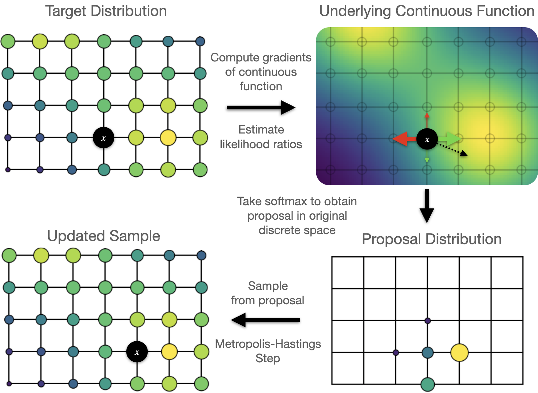
Figure 1: Our approach visualized. Often discrete distributions are defined by continuous functions whose input is restricted to a discrete set; here $R^{2}$ restricted to $\mathcal{Z}^{2}$. We use a Taylor series computed on the underlying continuous function to estimate likelihood ratios of making discrete moves; here $\pm 1$ in either direction. These estimated likelihood ratios are used to inform a proposal distribution over moves in the original discrete space.

In search for a unifying structure, we notice that many discrete distributions are written (and implemented) as differentiable functions of real-valued inputs. The discrete structure is created by restricting the continuous inputs to a discrete subset of their domain. In this paper, we use the gradients of these underlying continuous functions to inform proposal distributions for MCMC sampling in large discrete probabilistic models. This new family of gradient-informed proposals for MCMC may be seen as a class of adaptive Gibbs samplers or a fast approximation to locally-informed proposals (Umrigar, 1993; Liu, 1996; Zanella, 2020).

As we show, this gradient information is cheaply available for many discrete distributions and can lead to orders of magnitude improvements in sampling efficiency. In some cases, it even outperforms samplers that exploit hard-coded independence structure.

We apply these sampling techniques to improve parameter inference in discrete energy-based models such as Ising and Potts models. We also find that our method is particularly well-suited to sample from unnormalized discrete distributions parameterized by deep neural networks. The improved efficiency of our sampler allows us to apply many techniques from large-scale continuous EBMs to successfully train deep EBMs for discrete data. These models are simple to define, flexible, and outperform baseline variational auto-encoders (Kingma & Welling, 2013) and existing energy-based models.

2 Background

In this work we are concerned with sampling from unnormalized distributions over discrete data

$$\log p(x)=f(x)-\log Z$$

where $f(x)$ is the unnormalized log-probability of $x$ and ${Z=\sum_{x}e^{f(x)}}$ is the normalizing constant which we assume is unknown. We restrict our study to $D$-dimensional binary $x\in\{0,1\}^{D}$ and categorical $x\in\{0,1,\ldots,K\}^{D}$ data as all finite-dimensional discrete distributions can be embedded in this way. Throughout the paper we assume all categorical variables are one-hot encoded.

2.1 Gibbs Sampling

Gibbs sampling is perhaps the simplest and most generic method for sampling from discrete distributions. At each step, the sampler partitions the dimensions of an input $x$ into two groups $x_{u}$ and $x_{-u}$ where $u$ is a subset of the $D$ dimensions of $x$ and $-u$ is its complement. The next sample in the chain is created by updating $x_{u}$ to be a sample from $p(x_{u}|x_{-u})$, the conditional distribution of the chosen dimensions, given all others. In some distributions, block-independence structure exists, making certain partitions easy to sample from and update in parallel.

In the worst case, if such structure does not exist, we can let $x_{u}=x_{i}$, simply the $i$-th dimension of $x$. In this setting $p(x_{i}|x_{-i})$ is simply a one-dimensional categorical distribution over $K$ possible outcomes, which requires $K$ evaluations of the unnormalized log-density function. We typically fix an ordering of the dimensions and iterate through this ordering to ensure that each dimension is updated.

While simple, updating one dimension at a time can be problematic for high-dimensional data. Consider for example a binary model of the MNIST dataset. Almost all dimensions will represent the background and if chosen for a Gibbs update, they will almost certainly not change. Similarly, the pixels on the interior of a digit will also not change. This amounts to wasted computation every time we propose a dimension, which does not change. Ideally, if we could bias our partition choice to dimensions which are likely to change, we could build a more efficient Gibbs sampler.

Consider a similar sampler for the binary case; Metropolis-Hastings with the proposal distribution ${q(x^{\prime}|x)=\sum_{i}q(x^{\prime}|x,i)q(i)}$ where $q(i)$ is a distribution over indices $i\in\{1,\ldots,D\}$ and $q(x^{\prime}|x,i)=\delta(x^{\prime}=x_{-i})$, where $\delta(\cdot)$ is the Dirac-delta distribution. With this sampler we will first sample an index $i\sim q(i)$, then flip the $i$-th bit of $x$ to obtain $x^{\prime}$ and accept this proposed update with probability

$$\min\left\{\exp(f(x^{\prime})-f(x))\frac{q(x|x^{\prime})}{q(x^{\prime}|x)},1\right\}.$$ (1)

This approach can lead to considerable performance improvements if $q(i)$ is biased towards dimensions which are more likely to flip. To this end, considerable work has been done to use prior sampling data to adaptively update the $q(i)$ while maintaining the validity of MCMC sampling (Łatuszyński et al., 2013; Richardson et al., 2010).

Revisiting our MNIST example, we can see the pixels most likely to change are those at the edge of a digit. Where this edge is varies considerably and depends on the entire input $x$. Thus, we can imagine an input dependent proposal $q(i|x)$ should be able to outperform an unconditional proposal $q(i)$. Our proposed approach does exactly that, using gradient information to inform a proposal over dimensions which leads to more efficient sampling.

2.2 Locally-Informed Proposals

A good Metropolis-Hastings proposal needs to balance the increase in the likelihood of the proposed point $x^{\prime}$ with the decrease in the probability of the reverse proposal $q(x|x^{\prime})$. A natural strategy for increasing the likelihood is to use locally-informed proposals:

$$q_{\tau}(x^{\prime}|x)\propto e^{\frac{1}{\tau}(f(x^{\prime})-f(x))}\mathbf{1}(x^{\prime}\in H(x)).$$ (2)

where $H(x)$ is the Hamming ball of some size around $x$ and $\tau>0$ is a temperature parameter. In this case, the proposal is simply a tempered Softmax over ${f(x^{\prime})-f(x)}$ for all $x^{\prime}\in H(x)$. If the temperature $\tau$ is too low, this proposal will aggressively optimize the local likelihood increase from $x\to x^{\prime}$, but possibly collapse the reverse proposal probability $q_{\tau}(x|x^{\prime})$. If the temperature $\tau$ is too high, this proposal may increase the reverse proposal probability $q_{\tau}(x|x^{\prime})$, but ignore the local likelihood increase.

The temperature that balances both of these terms is $\tau=2$ (Umrigar, 1993; Zanella, 2020). We include a derivation of this fact in Appendix A. In fact, Zanella (2020) showed that $q_{2}(x^{\prime}|x)$ is in the optimal subclass of locally-informed proposals. Zanella (2020) also demonstrated that this can lead to large improvements in empirical performance per sampling step compared to other generic samplers like Gibbs and the Hamming-Ball sampler (Titsias & Yau, 2017).

Unfortunately, while powerful, these locally-informed proposals requires us to compute $f(x^{\prime})-f(x)$ for every $x^{\prime}\in H(x)$. For $D$-dimensional data and a Hamming window size of 1, this requires $\mathcal{O}(D)$ evaluations of $f$ which can become prohibitive as $D$ grows. Our proposed approach reduces this to $\mathcal{O}(1)$ evaluations while incurring a minimal decrease in the efficiency of each sampling step.

3 Searching for Structure

For some distributions, structure exists which enables the local differences $f(x^{\prime})-f(x)$ to be computed efficiently. This is not true in general, but even in settings where it is, bespoke derivations and implementations are required. Ideally, we could identify a structure that is ubiquitous across many interesting discrete distributions, can be exploited in a generic and generalizable way, and can allow us to accurately estimate the local differences.

To find such structure, we examine the functional form of the unnormalized log-probability for some common, diverse families of discrete distributions in Table 1.

Distribution	$\log p(x)+\log Z$
Categorical	$x^{T}\theta$
Poisson	$x\log\lambda-\log\Gamma(x+1)$
HMM	$\sum_{t=1}^{T}x_{t+1}^{T}Ax_{t}-\frac{(w^{T}x-y)^{2}}{2\sigma^{2}}$
RBM	$\sum_{i}\text{softplus}(Wx+b)_{i}+c^{T}x$
Ising	$x^{T}Wx+b^{T}x$
Potts	$\sum_{i=1}^{L}h_{i}^{T}x_{i}+\sum_{i,j=1}^{L}x_{i}^{T}J_{ij}x_{j}$
Deep EBM	$f_{\theta}(x)$

Table 1: Unnormalized log-likelihoods of common discrete distributions. All are differentiable with respect to $x$.

The formulas in Table 1 are not only the standard way these distributions are written down, but they are also the standard way these distributions are implemented in probabilisitic programming frameworks.

The key insight here is that these are all continuous, differentiable functions accepting real-valued inputs, even though they are evaluated only on a discrete subset of their domain. We propose to exploit this structure and that gradients, in the form of Taylor-series approximations, can be used to efficiently estimate likelihood ratios between a given input $x$ and other discrete states $x^{\prime}$.

When we are dealing with $D$-dimensional binary data, we can estimate the likelihood ratios of flipping each bit with

$$\tilde{d}(x)=-(2x-1)\odot\nabla_{x}f(x)$$ (3)

where $\tilde{d}(x)_{i}\approx f(x_{-i})-f(x)$ and $x_{-i}$ is $x$ with the $i$-th bit flipped. If we are dealing with $D$-dimensional categorical data we can estimate a similar quantity

$$\tilde{d}(x)_{ij}=\nabla_{x}f(x)_{ij}-x_{i}^{T}\nabla_{x}f(x)_{i}$$ (4)

where $\tilde{d}(x)_{ij}$ approximates the log-likelihood ratio of flipping the $i$-th dimension of $x$ from its current value to the value $j$. Similar first-order approximations can easily be derived for larger window sizes as well with linear operators applied to the gradient of the log-probability function.

We note, there may be many different underlying continuous functions which correspond to a given discrete distribution. We later present theory (Theorem 1) which can guide this choice in settings where there is any ambiguity.

4 Gibbs With Gradients

We now present our main algorithm. We use a Taylor-series (Equations 3, 4) to approximate the likelihood ratios within a local window of a point $x$. We use these estimated likelihood ratios to produce an approximation

$$q^{\nabla}(x^{\prime}|x)\propto e^{\frac{\tilde{d}(x)}{2}}\mathbf{1}(x^{\prime}\in H(x))$$ (5)

to $q_{2}(x^{\prime}|x)$ of Equation 2, which we use in the standard Metropolis-Hastings algorithm.

Our experiments focus on a simple and fast instance of this approach which only considers local moves inside of a Hamming window of size 1. For binary data, these window-1 proposals have an even simpler form since all $x^{\prime}\in H(x)$ differ by only dimension. Proposing a move from $x$ to $x^{\prime}$ is equivalent to choosing which dimension $i$ to change. We can sample this from a categorical distribution over $D$ choices:

$$q(i|x)=\text{Categorical}\left(\text{Softmax}\left(\frac{\tilde{d}(x)}{2}\right)\right)$$ (6)

Thus when $x$ binary, to sample from $q^{\nabla}(x^{\prime}|x)$, we simply sample which dimension to change $i\sim q(i|x)$, and then deterministically set $x^{\prime}=\textnormal{{flipdim}}(x,i)$. In this case, when $x$ and $x^{\prime}$ differ only in dimension $i$, we have $q^{\nabla}(x^{\prime}|x)=q(i|x)$ and $q^{\nabla}(x|x^{\prime})=q(i|x^{\prime})$.

Because of the relationship to Adaptive Gibbs, we call our sampler Gibbs-With-Gradients (GWG). Pseudo-code describing our sampler can be found in Algorithm 1.

Algorithm 1 Gibbs With Gradients

  Input: unnormalized log-prob $f(\cdot)$, current sample $x$

  Compute $\tilde{d}(x)$ {Eq. 3 if binary, Eq. 4 if categorical.}

  Compute $q(i|x)=\text{Categorical}\left(\text{Softmax}\left(\frac{\tilde{d}(x)}{2}\right)\right)$

  Sample $i\sim q(i|x)$

  $x^{\prime}=\textnormal{{flipdim}}(x,i)$

  Compute $q(i|x^{\prime})=\text{Categorical}\left(\text{Softmax}\left(\frac{\tilde{d}(x^{\prime})}{2}\right)\right)$

  Accept with probability:

$$\min\left(\exp(f(x^{\prime})-f(x))\frac{q(i|x^{\prime})}{q(i|x)},1\right)$$

In the categorical data setting, the proposal must choose not only which dimension to change, but also to what value. Thus, $q(i|x)$ in this setting is a $D(K-1)$-way Softmax.

We describe some simple extensions in Appendix D and code to replicate our experiments is available here.

4.1 Analyzing Approximations

Zanella (2020) proved that “locally-balanced” proposals, like $q_{2}(x^{\prime}|x)$ in Equation 2, are the optimal locally-informed proposals for Metropolis-Hastings. In this section we show that, under smoothness assumptions on $f$, our methods are within a constant factor of $q_{2}(x^{\prime}|x)$ in terms of asymptotic efficiency.

To understand the asymptotic efficiency of MCMC transition kernels, we can study the asymptotic variance and spectral gap of the kernel. The asymptotic variance is defined as

$$\text{var}_{p}(h,Q)=\lim_{T\rightarrow\infty}\frac{1}{T}\text{var}\left(\sum_{t=1}^{T}h(x_{t})\right)$$ (7)

where $h:\mathcal{X}\rightarrow R$ is a scalar-valued function, $Q$ is a $p$-stationary Markov transition kernel, and ${X_{1}\sim p(x)}$. The spectral gap is defined as

$$\text{Gap}(Q)=1-\lambda_{2}$$ (8)

where $\lambda_{2}$ is the second largest eigenvalue of the transition probability matrix of $Q$. Both of these quantities measure the asymptotic efficiency of $Q$. The asymptotic variances measures the additional variance incurred when using sequential samples from $Q$ to estimate $E_{p}[h(x)]$. For transition probability matrices with non-negative eigenvalues, the spectral gap is related to the mixing time, with larger values corresponding to faster mixing chains (Levin & Peres, 2017).

Since our method approximates $q_{2}(x^{\prime}|x)$, we should expect some decrease in efficiency. We characterize this decrease in terms of the asymptotic variance and spectral gap, under the assumption of Lipschitz continuity of $\nabla_{x}f(x)$. In particular, we show that the decrease is a constant factor that depends on the Lipschitz constant of $\nabla_{x}f(x)$ and the window size of our proposal.

Theorem 1

Let $Q(x^{\prime},x)$ and $Q^{\nabla}(x^{\prime},x)$ be the Markov transition kernels given by the Metropolis-Hastings algorithm using the locally balanced proposal $q_{2}(x^{\prime}|x)$ and our approximation $q^{\nabla}(x^{\prime}|x)$. Let $f$ be an $L$-smooth log-probability function and $p(x)=\frac{\exp(f(x))}{Z}$. Then it holds

1. $\text{var}_{p}(h,Q^{\nabla})\leq\frac{\text{var}_{p}\left(h,Q\right)}{c}+\frac{1-c}{c}\cdot\text{var}_{p}(h)$

2. $\text{Gap}(Q^{\nabla})\geq c\cdot\text{Gap}\left(Q\right)$

where $c=e^{-\frac{1}{2}LD_{H}^{2}}$ and $D_{H}=\sup_{x^{\prime}\in H(x)}||x-x^{\prime}||$.

A proof can be found in Appendix B. This roughly states that $Q^{\nabla}(x^{\prime},x)$ is no less than $c$-times as efficient than $Q(x^{\prime},x)$ per step for estimating expectations. As expected, our approach matches the efficiency of the target proposal when the Taylor-series approximation is accurate. We can derive from Theorem 1 that when considering which functional representation of our distribution to choose, we should choose the representation whose gradient has the smallest Lipschitz constant.

An example:

Consider an Ising model on a cyclic 2D lattice. This model has log-probability function ${f(x)=\theta\cdot x^{T}Jx-\log Z}$ where $J$ is the binary adjacency matrix of the lattice, $\theta$ is the connectivity strength and $Z$ is the unknown normalizing constant. We can see the gradient is $\nabla_{x}f(x)=2\theta\cdot Jx$ and can bound $L\leq 2\sigma(J)\theta=8\theta$.

For $\theta=.1$ and a Hamming window of size 1, this gives $c=.67$, regardless of $D$. Since a single evaluation of $f$ has an $\mathcal{O}(D^{2})$ cost, it costs $\mathcal{O}(D^{3})$ to compute $q_{2}(x^{\prime}|x)$. Compared to the exact local-differences proposal, the Gibbs-With-Gradients proposal $q^{\nabla}(x^{\prime}|x)$ incurs at most a constant loss in sampling efficiency per-iteration but gives a $\mathcal{O}(D)$ increase in speed.

5 Relationship to Continuous Relaxations

Why hasn’t this relatively simple approach been proposed before? A number of prior works have used gradient information for discrete sampling. Instead of using gradients to inform discrete updates directly, these methods transport the problem into a continuous relaxation, perform updates there, and transform back after sampling. This approach incurs many of the pitfalls of continuous sampling without providing the scalability. We find these methods are not competitive with Gibbs-With-Gradients in high dimensions.

In more detail, these methods use the discrete target distribution to create a related continuous distribution (relaxation) whose samples can be transformed to samples from the target distribution. They then apply gradient-based sampling methods such as Stein Variational Gradient Descent (Liu & Wang, 2016) or Hamiltonian Monte-Carlo (HMC) (Neal et al., 2011) to the new distribution. Examples of such methods are the recently proposed Discrete-SVGD (D-SVGD) (Han et al., 2020) and Discontinuous HMC (Nishimura et al., 2017).

A key challenge of these approaches is that the relaxed distribution can be arbitrarily difficult to sample from, highly multi-modal and require small step-sizes. Further, metrics of MCMC performance and mixing in the relaxed space may not indicate performance and mixing in the discrete space. These methods also require the tuning of many additional hyper-parameters such as step-size, momentum, and the temperature of the relaxation. In contrast, our approach operates directly in discrete space, and has no hyper-parameters.

Figure 2 compares these approaches on the task of sampling from restricted Boltzmann machines (RBMs) of up to 1000 dimensions. We compare to D-SVGD and two relaxation-based baselines derived from the Metropolis-Adjusted Langevin Algorithm (Besag, 1994) and HMC. We compare the log-MMD between generated samples and “ground-truth” samples generated with Block-Gibbs. We also display samples from an MNIST-trained model. In contrast to all three baselines, our approach does not degrade with dimension. Additional results, details, and discussion can be found in Appendix C. These relaxation-based approaches do not scale beyond 200 dimensions, so we do not compare to them in our main experimental results section

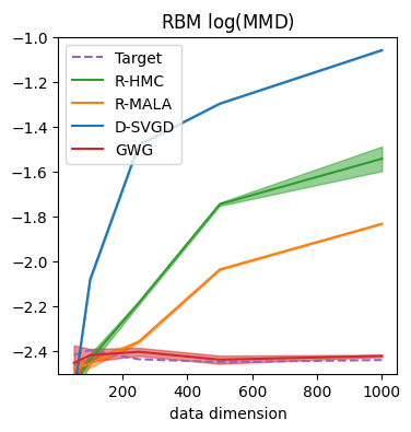
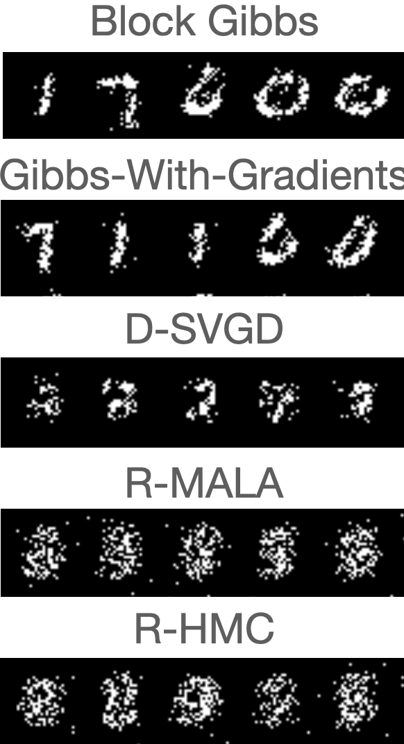
Figure 2: Comparison to gradient-based samplers with continuous relaxations. GWG, D-SVGD, R-HMC, and R-MALA refer to Gibbs-With-Gradients, Discrete SVGD, Relaxed HMC and Relaxed MALA, respectively. Left: Log-MMD (lower is better) between true samples and generated samples for RBMs of increasing dimension (over 3 runs). “Target” is log-MMD between two sets of Block-Gibbs samples. Right: Visualized samples from an RBM trained on MNIST.

6 Sampling From EBMs

To demonstrate the benefits and generality of our proposed approach to sampling, we present results sampling from 3 distinct and challenging distributions; Restricted Boltzmann Machines, Lattice Ising models, and Factorial Hidden Markov Models. Each is evaluated differently based on the properties of the distribution. We compare our sampler, Gibbs-With-Gradients, against standard Gibbs sampling and the Hamming Ball Sampler (Titsias & Yau, 2017) – two generic approaches for discrete sampling. When available, we also compare with samplers which exploit known structure in the distribution of interest.

In the following, Gibbs-$X$ refers to Gibbs sampling with a block-size of $X$, and HB-$X$-$Y$ refers to the Hamming Ball sampler with a block size of $X$ and a hamming ball size of $Y$, and GWG refers to Gibbs-With-Gradients. Gibbs-1 is the fastest sampler tested. In our current implementation, we find Gibbs-2, HB-10-1, and GWG have approximately 1.6, 6.6, 2.1 times the cost of Gibbs-1 per step, respectively. Thus the run-time of GWG is most comparable to Gibbs-2.

Restricted Boltzmann Machines

are unnormalized latent-variable models defined as:

$$\log p(x)=\log(1+\exp(Wx+c))+b^{T}x-\log Z$$ (9)

where $\{W,b,c\}$ define its parameters and $x\in\{0,1\}^{D}$. We train an RBM with 500 hidden units on the MNIST dataset using contrastive divergence (Hinton, 2002). We generate samples with various MCMC samplers and compare them in two ways. First, using the Maximum Mean Discrepancy (MMD) (Gretton et al., 2012) between a set of samples from each sampler and a set of “ground-truth” samples generated using the structured Block-Gibbs sampler available to RBMs (see Appendix E for details). Next, we report the Effective Sample Size (ESS) of a summary statistic over sampling trajectories. Results can be seen in Figure 3.

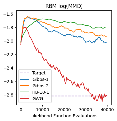
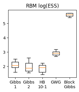
Figure 3: RBM sampling results. Left: Log-MMD of samples over steps (lower is better). “Target” is Log-MMD between two sets of Block-Gibbs samples. Right: Log-ESS of various samplers after 10,000 steps. Gibbs-With-Gradients matches Block-Gibbs in MMD and outperforms unstructured baselines in ESS.

We see on the left that GWG matches the structured Block-Gibbs sampler in MMD (“Target” in the Figure), while the other samplers do not. On the right we see that the effective sample size of GWG is notably above the baselines and is approximately halfway between the baselines and the Block-Gibbs sampler (in log-space). We note, Block-Gibbs can update all 784 dimensions in each iterations. GWG and Gibbs-1 can update 1 and Gibbs-2 and Hamming Ball can update 2 dimensions per iteration.

Lattice Ising Models

are models for binary data defined by

$$\log p(x)=\theta\cdot x^{T}Jx-\log Z$$ (10)

where $\theta$ is the connectivity strength and $J$ is the binary adjacency matrix, here restricted to be a 2D cyclic lattice. This model was originally proposed to model the spin magnetic particles (Ising, 1924). We sample from models with increasing dimension and connectivity strength. We evaluate using Effective Sample Size (ESS) of a summary statistic (full details in Appendix F). Results can be seen in Figure 4.

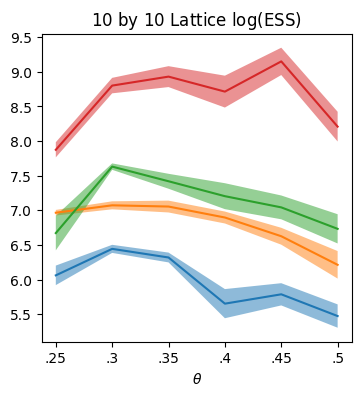
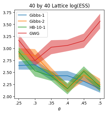
Figure 4: Ising model sampling results. The y-axis shows log-ESS over 100,000 samples steps. Left: 10x10 lattice, right: 40x40 lattice. We see Gibbs-With-Gradients (GWG) outperforms in most settings.

We see Gibbs-With-Gradients provides a notable increase in ESS for Ising models with higher connectivity. These models are harder to sample from as their dimensions are more correlated.

Factorial Hidden Markov Models

(FHMM) are latent-variable time-series models, similar to HMMs but their hidden state consists of distinct, independent factors. The continuous data $y\in R^{L}$ of length $L$ is generated by the binary hidden state $x\in\{0,1\}^{L\times K}$ with $K$ factors as

$$p(x,y) =p(y|x)p(x)$$

$$p(y|x) =\prod_{t=1}^{L}\mathcal{N}(y_{t};Wx_{t}+b,\sigma^{2})$$

$$p(x) =p(x_{1})\prod_{t=2}^{L}p(x_{t}|x_{t-1})$$ (11)

We create a random FHMM with 1000 time-steps and a 10-dimensional hidden state and then draw samples $y$. We generate posterior samples $p(x|y)$ and evaluate our samplers using reconstruction error and joint likelihood. Full model description and experimental details can be found in Appendix G and results can be seen in Figure 5.

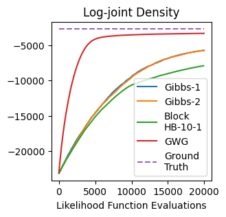
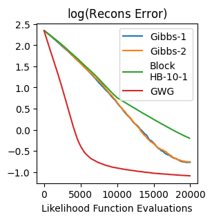
Figure 5: Factorial Hidden Markov Model results. “Block-HB” refers to the block-structured hamming ball sampler. Left, log-joint density and right, mean log-reconstruction error. GWG performs best in both evaluations, outperforming the Hamming Ball sampler which exploits model structure.

In this setting, the Hamming-Ball sampler exploits known structure in the problem. Each block chosen by the sampler consists of the 10-dimensional latent state $x_{t}$, as opposed to 10 random dimensions. Thus, the Hamming-Ball sampler in this setting is a stronger baseline. Despite this, we find Gibbs-With-Gradients notably outperforms the baseline samplers.

7 Training EBMs

Training EBMs is a challenging task. Computing the likelihood for Maximum Likelihood inference requires computation of the normalizing constant ${Z=\sum_{x}e^{f_{\theta}(x)}}$ which is typically intractable. Thankfully, the gradient of the log-likelihood can be more easily expressed as:

$$\nabla_{\theta}\log p(x)=\nabla_{\theta}f_{\theta}(x)-E_{p(x)}[\nabla_{\theta}f_{\theta}(x)]$$ (12)

therefore, if samples can be drawn from $p(x)$, then an unbiased gradient estimator can be derived. We can approximate this estimator using MCMC. When a slow-mixing MCMC sampler is used to draw these samples, we obtain biased gradient estimates and this leads to sub-par learning. Improvements in MCMC can then lead to improvements in parameter inference for unnormalized models. We explore how Gibbs-With-Gradients can be applied to parameter inference for some classical discrete EBMs.

7.1 Training Ising models on generated data

We generate Ising models with different sparse graph structures; a 2D cyclic lattice and a random Erdos-Renyi graph. We generate training data with a long-run Gibbs chain and train models using Persistent Contrastive Divergence (Tieleman, 2008) with an $\ell 1$ penalty to encourage sparsity. We evaluate our models using the Root-Mean-Squared-Error (RMSE) between the inferred connectivity matrix $\hat{J}$ and the true matrix $J$.

Full experimental details and additional results can be found in Appendix F.2, F.3 and results can be seen in Figure 6. In all settings, GWG greatly outperforms Gibbs sampling. This allows for much faster training than standard Gibbs while recovering higher-quality solutions.

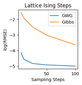
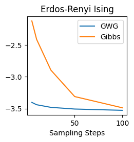
Figure 6: Training Ising models with increasing MCMC steps. Left: Lattice Ising (dim = 625, $\theta=.25$). Right: Erdos-Renyi Ising. Values are $\log$(RMSE) between the learned and true $J$. GWG leads to better solutions with lower computational cost.

7.2 Protein Coupling Prediction with Potts Models

Proteins are defined by a discrete sequence of 20 amino acids $x\in\{1,\ldots,20\}^{D}$ where $D$ is the length of the protein. The Potts model has long been a popular approach for modelling the evolutionary distribution of protein sequences (Lapedes et al., 1999). The model takes the form

$$\log p(x)=\sum_{i=1}^{D}h_{i}^{T}x_{i}+\sum_{i,j=1}^{D}x_{i}^{T}J_{ij}x_{j}-\log Z$$ (13)

where $x_{i}$ is a one-hot encoding of the $i$-th amino acid in $x$, $J\in R^{\{D\times D\times 20\times 20\}}$ and $h\in R^{\{D\times 20\}}$ are the model’s parameters and $Z$ is the model’s normalizing constant. The Potts model’s likelihood is the sum of pairwise interactions. Marks et al. (2011) demonstrated that the strength of these interactions can correspond to whether or not two amino acids touch when the protein folds. These inferred contacts can then be used to infer the 3D structure of the protein.

Since the Potts model is unnormalized, maximum likelihood learning is difficult, and $\ell 1$-regularized Pseudo-likelihood Maximization (PLM) (Besag, 1975) is used to train the model. Recently Ingraham & Marks (2017) found that improved contact prediction could be achieved with MCMC-based maximum likelihood learning. Unfortunately, due to the limitations of discrete MCMC samplers, their study was restricted to small proteins (less than 50 amino acids).

GWG allows these performance improvements to scale to large proteins as well. We train Potts models on 2 large proteins: OPSD_BOVIN, and CADH1_HUMAN. We train using PCD where samples are generated with GWG and Gibbs. We run PLM as a baseline. These proteins are much larger than those studied in Ingraham & Marks (2017) with OPSD_BOVIN, and CADH1_HUMAN having 276, and 526 amino acids, respectively.

We predict couplings using the $J$ parameter of our models. We compute a “coupling-strength” for each pair of amino-acids as $||J_{ij}||_{2}$ which gives a measure of how much indices $i$ and $j$ interact to determine the fitness of a protein. We sort index pairs by their coupling strength and compare the highest scoring pairs with known contacts in the proteins.

Full experimental details and additional results can be found in Appendix H and results can be seen in Figure 7. For the smaller protein, Gibbs sampling outperforms PLM but for the larger protein, the slow-mixing of the sampler causes the performance to drop below that of PLM. Despite the increased size, Gibbs-With-Gradients performs the best.

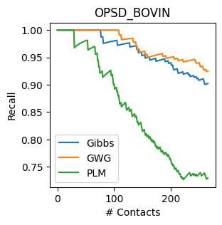
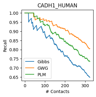
Figure 7: Recall Curves for contact prediction with Potts models. Gibbs-With-Gradients leads to higher recall.

Data Type	Dataset	VAE	VAE	EBM	EBM	RBM	DBN
		(MLP)	(Conv)	(GWG)	(Gibbs)
Binary	Static MNIST	-86.05	-82.41	-80.01	-117.17	-86.39	-85.67
	Dynamic MNIST	-82.42	-80.40	-80.51	-121.19	—	—
(log-likelihood $\uparrow$)	Omniglot	-103.52	-97.65	-94.72	-142.06	-100.47	-100.78
	Caltech Silhouettes	-112.08	-106.35	-96.20	-163.50	—	—
Categorical	Frey Faces	4.61	4.49	4.65	—	—	—
(bits/dim $\downarrow$)	Histopathology	5.82	5.59	5.08	—	—	—

Table 2: Test-set log-likelihoods for models trained on discrete image datasets. RBM and DBN results are taken from Burda et al. (2015), VAE results taken from Tomczak & Welling (2018).

8 Deep EBMs for Discrete Data

Deep Energy-Based Models have rapidly gained popularity for generative modeling. These models take the form

$$\log p(x)=f_{\theta}(x)-\log Z$$ (14)

where $f_{\theta}:R^{D}\rightarrow R$ is a deep neural network. The recent success of these models can be attributed to a few advancements including; the use of tempered Langevin samplers (Nijkamp et al., 2020) and large persistent chains (Du & Mordatch, 2019). This has enabled EBMs to become a competitive approach for image-generation (Song & Ermon, 2019), adversarial robustness (Grathwohl et al., 2019; Hill et al., 2020), semi-supervised learning (Song & Ou, 2018; Grathwohl et al., 2020a) and many other problems.

These advances rely on gradient-based sampling which requires continuous data. Thus, these scalable methods cannot be applied towards training deep EBMs on discrete data. We explore how Gibbs-With-Gradients can enable the training of deep EBMs on high-dimensional binary and categorical data. To our knowledge, models of this form have not be successfully trained on such data in the past. We train deep EBMs parameterized by Residual Networks (He et al., 2016) on small binary and continuous image datasets using PCD (Tieleman, 2008) with a replay buffer as in Du & Mordatch (2019); Grathwohl et al. (2019). The continuous images were treated as 1-of-256 categorical data.

PCD training is very sensitive to the choice of MCMC sampler. As an initial experiment, we attempted to train these models using standard Gibbs but found that the sampler was too slow to enable stable training within a reasonable compute budget. On the binary data we needed to train with 800 Gibbs sampling steps per training iteration. All models we trained with fewer steps quickly diverged. GWG required only 40. This made training with Gibbs 9.52x slower than GWG. For a fair comparison, the Gibbs results in Table 2 were trained for an equal amount of wall-clock time as the GWG models.

For the categorical data, we could not train models with Gibbs sampling. Each step of Gibbs requires us to evaluate the energy function 256 (for each possible pixel value) times. GWG requires 2 function evaluations. Thus the amount of compute per iteration for Gibbs is 128x greater than GWG. Further, to make Gibbs train stably, we would need to use many more steps, as with the binary data. This would give roughly a 870x increase in run-time. Therefore, training a model of this form with Gibbs is simply not feasible.

Full experimental details can be found in Appendix I. We present long-run samples from our trained models in Figure 8 and test-set likelihoods in Table 2. Likelihoods are estimated using Annealed Importance Sampling (Neal, 2001). We compare the performance of our models to Variational Autoencoders (Kingma & Welling, 2013) and two other EBMs; an RBM and a Deep Belief Network (DBN) (Hinton, 2009). On most datasets, our Resnet EBM outperforms the other two EBMs and the VAEs. Our improved sampler enables deep EBMs to become a competitive approach to generative modeling on high-dimensional discrete data.

We include some preliminary results using Gibbs-With-Gradients to train EBMs for text data in Appendix J.

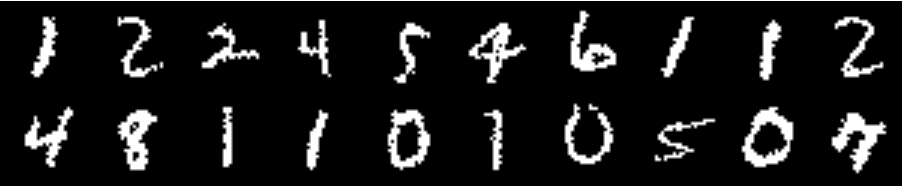
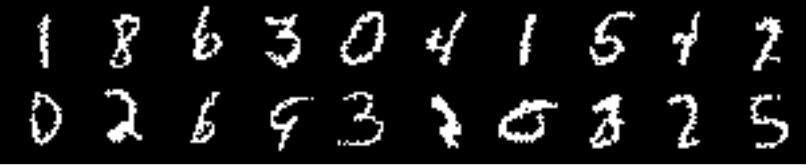
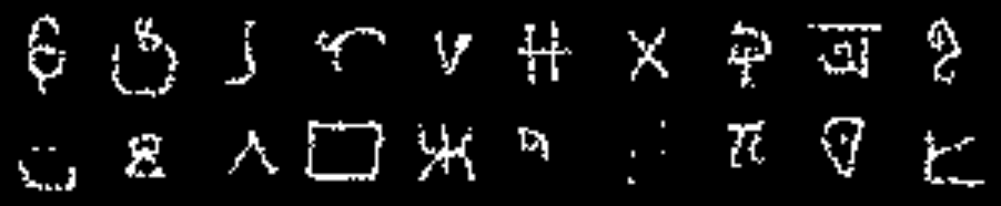
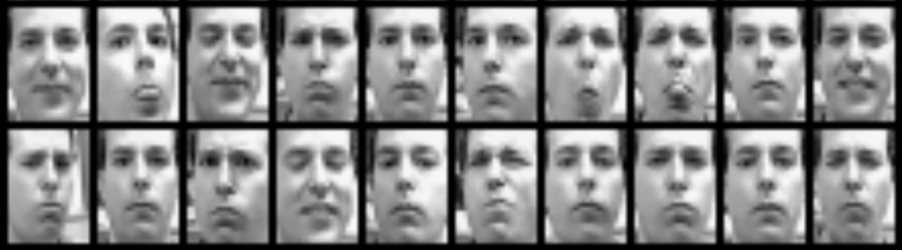
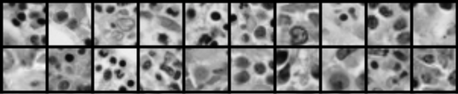
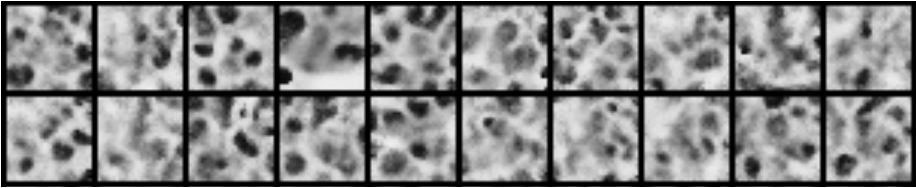
Figure 8: Left: data. Right: Samples from ResNet EBM. Samples generated with annealed Markov chain using 300,000 Gibbs-With-Gradients steps. Top to bottom: MNIST, omniglot, Caltech Silhouettes, Frey Faces, Histopathology.

9 Future Directions and Conclusion

In this work we have presented Gibbs-With-Gradients, a new approach to MCMC sampling for discrete distributions. Our approach exploits a powerful structure, gradient information, which is available to a very large class of important discrete distributions. We then use this gradient information to construct proposal distributions for Metropolis-Hastings.

We have demonstrated on a diverse set of distributions that this approach to sampling considerably outperforms baseline samplers which do not exploit known structure in the target distribution as well as many that do. Further, we find our approach outperforms prior discrete samplers which use gradient information with continuous relaxations.

We find Gibbs-With-Gradients performs very well at sampling from deep energy-based models and allows, for the first time, unconstrained deep EBMs to be trained on discrete data and outperform other deep generative models.

We believe there is considerable room for future work building on top of our method. We only explored samplers which modify 1 variable per proposed update. We believe considerable improvements could be made if the window size of the sampler was expanded but this would require more efficient algorithms to sample from the larger proposal.

Next, we have shown that gradient-based approximations to the local difference function can be accurate and useful for complex discrete distributions. Local difference functions have been used in the past to generalize Score Matching (Lyu, 2012), and Stein Discrepancies (Han & Liu, 2018). We believe there is great potential to explore how gradient-based approximations could enable the generalization of recent deep EBM training methods based on Score Matching and Stein Discrepancies (Song & Ermon, 2019; Grathwohl et al., 2020b) to models of discrete data.

10 Acknowledgements

We would like to thank Eli Weinstein for helping us properly present our protein model results and we would like to thank Kelly Brock for help and feedback for working with the protein data. We thank Jesse Bettencourt, James Lucas, and Jacob Kelly for helpful feedback on our draft. Last, we would like to thank Jeffrey Rosenthal for providing information on related methods and prior work.

Appendix A Balancing Locally-Informed Proposals

As discussed in Section 2.2, locally informed proposals need to balance the likelihood increase with the reverse proposal probability. In particular, consider proposals of the form:

$$q_{\tau}(x^{\prime}|x)\propto e^{\frac{1}{\tau}(f(x^{\prime})-f(x))}\mathbf{1}(x^{\prime}\in H(x)).$$ (15)

where $H(x)$ is the Hamming ball of some size around $x$ and $\tau>0$ is a temperature parameter. Here we provide a derivation of the fact that $\tau=2$ balances these two terms.

When we examine the acceptance rate (Equation 1) of this proposal we find

$$\exp( f(x^{\prime})-f(x))\frac{q_{\tau}(x|x^{\prime})}{q_{\tau}(x^{\prime}|x)}$$

$$=\exp(f(x^{\prime})-f(x))\frac{\exp(\frac{1}{\tau}(f(x)-f(x^{\prime}))Z(x)}{\exp(\frac{1}{\tau}(f(x^{\prime})-f(x))Z(x^{\prime})}$$

$$=\exp\left(\left(1-\frac{2}{\tau}\right)(f(x^{\prime})-f(x))\right)\frac{Z(x)}{Z(x^{\prime})}$$ (16)

where $Z(x)=\sum_{x^{\prime}\in H(x)}\exp(\frac{1}{\tau}(f(x^{\prime})-f(x))$ is the normalizing constant of the proposal. By setting $\tau=2$, the most variable terms cancel and we are left with $\frac{Z(x)}{Z(x^{\prime})}$. Thus, the acceptance rate is equal to the ratio of the normalizing constants of the proposal distributions. If the Hamming ball is small and the function $f$ is well behaved (i.e Lipschitz) then, since $x^{\prime}$ is near $x$, $Z(x^{\prime})$ will be near $Z(x)$ and the acceptance rate will be high.

Appendix B Proof of Theorem 1

Our proof follows from Theorem 2 of Zanella (2020) which states that for two $p$-reversible Markov transition kernels $Q_{1}(x^{\prime},x)$ and $Q_{2}(x^{\prime},x)$, if there exists $c>0$ for all $x^{\prime}\neq x$ such that $Q_{1}(x^{\prime},x)>c\cdot Q_{2}(x^{\prime},x)$ then

1. $\text{var}_{p}(h,Q_{1})\leq\frac{\text{var}_{p}(h,Q_{1})}{c}+\frac{1-c}{c}\cdot\text{var}_{p}(h)$

2. $\text{Gap}(Q_{1})\geq c\cdot\text{Gap}(Q_{2})$

where $\text{var}_{p}(h,Q)$ is the asymptotic variance defined in Equation 7, $\text{Gap}(Q)$ is the spectral gap defined in Equation 8, and $\text{var}_{p}(h)$ is the standard variance $E_{p}[h(x)^{2}]-E_{p}[h(x)]^{2}$.

Our proof proceeds by showing we can bound ${Q^{\nabla}(x^{\prime},x)\geq c\cdot Q(x^{\prime},x)}$, and the results of the theorem then follow directly from Theorem 2 of Zanella (2020).

B.1 Definitions

We begin by writing down the proposal distribution of interest and their corresponding Markov transition kernels. For ease of notion we define some values

$$\Delta(x^{\prime},x) \coloneqq f(x^{\prime})-f(x)$$

$$\nabla(x^{\prime},x) \coloneqq\nabla_{x}f(x)^{T}(x^{\prime}-x)$$

$$D_{H} \coloneqq\sup_{x^{\prime}\in H(x)}||x^{\prime}-x||$$

We restate the target proposal for $x^{\prime}\in H(x)$

$$q_{2}(x^{\prime}|x)=\frac{\exp\left(\frac{\Delta(x^{\prime},x)}{2}\right)}{Z(x)}$$

where we have defined

$$Z(x)=\sum_{x^{\prime}\in H(x)}\exp\left(\frac{\Delta(x^{\prime},x)}{2}\right).$$

This proposal leads to the Markov transition kernel

$$Q(x^{\prime},x) =q_{2}(x^{\prime}|x)\min\left\{1,\frac{Z(x)}{Z(x^{\prime})}\right\}$$

$$=\min\left\{\frac{\exp\left(\frac{\Delta(x^{\prime},x)}{2}\right)}{Z(x)},\frac{\exp\left(\frac{\Delta(x^{\prime},x)}{2}\right)}{Z(x^{\prime})}\right\}.$$

We now restate our approximate proposal for $x^{\prime}\in H(x)$

$$q^{\nabla}(x^{\prime}|x)=\frac{\exp\left(\frac{\nabla(x^{\prime},x)}{2}\right)}{\tilde{Z}(x)}$$

where we have defined

$$\tilde{Z}(x)=\sum_{x^{\prime}\in H(x)}\exp\left(\frac{\nabla(x^{\prime},x)}{2}\right)$$

which leads to the Markov transition kernel

$$Q {}^{\nabla}(x^{\prime},x)=$$

$$q^{\nabla}(x^{\prime}|x)\min\left\{1,\frac{\exp\left(\Delta(x^{\prime},x)\right)}{\exp\left(\frac{\nabla(x^{\prime},x)-\nabla(x,x^{\prime})}{2}\right)}\frac{\tilde{Z}(x)}{\tilde{Z}(x^{\prime})}\right\}$$

$$=\min\left\{\frac{\exp\left(\frac{\nabla(x^{\prime},x)}{2}\right)}{\tilde{Z}(x)},\frac{\exp\left(\Delta(x^{\prime},x)+\frac{\nabla(x,x^{\prime})}{2}\right)}{\tilde{Z}(x^{\prime})}\right\}.$$

B.2 Preliminaries

It can be seen that $\nabla(x^{\prime},x)$ is a first order Taylor-series approximation to $\Delta(x^{\prime},x)$ and it follows directly from the Lipschitz continuity of $\nabla_{x}f(x)$ that

$$|\nabla(x^{\prime},x)-\Delta(x^{\prime},x)|\leq\frac{L}{2}||x^{\prime}-x^{\prime}||^{2}$$ (17)

and since we restrict $x^{\prime}\in H(x)$ we have

$$-\frac{L}{2}D_{H}^{2}\leq\nabla(x^{\prime},x)-\Delta(x^{\prime},x)\leq\frac{L}{2}D_{H}^{2}$$ (18)

B.3 Normalizing Constant Bounds

We derive upper- and lower-bounds on $\tilde{Z}(x)$ in terms of $Z(x)$.

$$\tilde{Z}(x) =\sum_{x^{\prime}\in H(x)}\exp\left(\frac{\nabla(x^{\prime},x)}{2}\right)$$

$$=\sum_{x^{\prime}\in H(x)}\exp\left(\frac{\Delta(x^{\prime},x)}{2}\right)\exp\left(\frac{\nabla(x^{\prime},x)-\Delta(x^{\prime},x)}{2}\right)$$

$$\leq\sum_{x^{\prime}\in H(x)}\exp\left(\frac{\Delta(x^{\prime},x)}{2}\right)\exp\left(\frac{LD_{H}^{2}}{4}\right)$$

$$\leq\exp\left(\frac{LD_{H}^{2}}{4}\right)\sum_{x^{\prime}\in H(x)}\exp\left(\frac{\Delta(x^{\prime},x)}{2}\right)$$

$$=\exp\left(\frac{LD_{H}^{2}}{4}\right)Z(x)$$ (19)

Following the same argument we can show

$$\tilde{Z}(x) \geq\exp\left(\frac{-LD_{H}^{2}}{4}\right)Z(x).$$ (20)

B.4 Inequalities of Minimums

We show ${Q^{\nabla}(x^{\prime},x)\geq c\cdot Q(x^{\prime},x)}$ for ${c=\exp\left(\frac{-LD_{H}^{2}}{2}\right)}$. Since both

$$Q(x^{\prime},x)=\min\{a,b\}$$

and

$$Q^{\nabla}(x^{\prime},x)=\min\{a^{\nabla},b^{\nabla}\}$$

it is sufficient to show $a^{\nabla}\geq c\cdot a$ and $b^{\nabla}\geq c\cdot b$ to prove the desired result.

We begin with the $a$ terms

$$\frac{a^{\nabla}}{a} =\frac{\exp\left(\frac{\nabla(x^{\prime},x)}{2}\right)}{\tilde{Z}(x)}\frac{Z(x)}{\exp\left(\frac{\Delta(x^{\prime},x)}{2}\right)}$$

$$=\frac{Z(x)}{\tilde{Z}(x)}\exp\left(\frac{\nabla(x^{\prime},x)}{2}-\frac{\Delta(x^{\prime},x)}{2}\right)$$

$$\geq\exp\left(\frac{-LD_{H}^{2}}{4}\right)\exp\left(\frac{\nabla(x^{\prime},x)}{2}-\frac{\Delta(x^{\prime},x)}{2}\right)$$

$$\geq\exp\left(\frac{-LD_{H}^{2}}{4}\right)\exp\left(\frac{-LD_{H}^{2}}{4}\right)$$

$$=\exp\left(\frac{-LD_{H}^{2}}{2}\right)$$ (21)

Now the $b$ terms

$$\frac{b^{\nabla}}{b} =\frac{\exp\left(\Delta(x^{\prime},x)+\frac{\nabla(x,x^{\prime})}{2}\right)}{\tilde{Z}(x^{\prime})}\frac{Z(x^{\prime})}{\exp\left(\frac{\Delta(x^{\prime},x)}{2}\right)}$$

$$=\frac{Z(x^{\prime})}{\tilde{Z}(x^{\prime})}\frac{\exp\left(\Delta(x^{\prime},x)+\frac{\nabla(x,x^{\prime})}{2}\right)}{\exp\left(\frac{\Delta(x^{\prime},x)}{2}\right)}$$

$$=\frac{Z(x^{\prime})}{\tilde{Z}(x^{\prime})}\exp\left(\frac{\Delta(x^{\prime},x)}{2}+\frac{\nabla(x,x^{\prime})}{2}\right)$$

$$\geq\exp\left(\frac{-LD_{H}^{2}}{4}\right)\exp\left(\frac{\Delta(x^{\prime},x)}{2}+\frac{\nabla(x,x^{\prime})}{2}\right)$$

$$=\exp\left(\frac{-LD_{H}^{2}}{4}\right)\exp\left(\frac{\nabla(x,x^{\prime})}{2}-\frac{\Delta(x,x^{\prime})}{2}\right)$$

$$\geq\exp\left(\frac{-LD_{H}^{2}}{4}\right)\exp\left(\frac{-LD_{H}^{2}}{4}\right)$$

$$=\exp\left(\frac{-LD_{H}^{2}}{2}\right)$$ (22)

B.5 Conclusions

We have shown that ${a^{\nabla}\geq\exp\left(\frac{-LD_{H}^{2}}{2}\right)a}$ and ${b^{\nabla}\geq\exp\left(\frac{-LD_{H}^{2}}{2}\right)b}$ and therefore it holds that

$$Q^{\nabla}(x^{\prime},x)\geq\exp\left(\frac{-LD_{H}^{2}}{2}\right)Q(x^{\prime},x)$$ (23)

From this, the main result follows directly from Theorem 2 of Zanella (2020).

Appendix C Relationship to Relaxations

Han et al. (2020) show that sampling from any discrete distribution can be transformed into sampling from a continuous distribution with a piece-wise density function. For simplicity we focus on a distribution $p(x)$ over binary data ${x\in\{0,1\}^{D}}$. To do this we will create a $D$-dimensional continuous distribution $p_{c}(z)$ where $z\in R^{D}$. We must specify a base distribution $p_{0}(z)$ which we choose to be $\mathcal{N}(0,I)$. We must then specify a function $\Gamma(z):R^{D}\rightarrow\{0,1\}^{D}$ which maps regions of equal mass under the base distribution to values in $\{0,1\}^{D}$. A natural choice is $\Gamma(z)=\text{sign}(z)$

We then define $p_{c}(z)$ as

$$p_{c}(z)=\mathcal{N}(z;0,I)p(\Gamma(z))$$

and it can be easily verified that generating

$$z\sim p_{c}(z),\qquad x=\Gamma(z)$$

will produce a sample from $p(x)$.

Thus, we have transformed a discrete sampling task into a task of sampling from a continuous distribution with a piece-wise density. Han et al. (2020) further relax this by defining

$$p^{\lambda}_{c}(x)=\mathcal{N}(z;0,I)p(\Gamma_{\lambda}(z))$$

where $\Gamma_{\lambda}(x)$ is a continuous approximation to $\Gamma(x)$. A natural choice for $\text{sign}(x)$ is a tempered sigmoid function

$$\Gamma_{\lambda}(x)=\frac{1}{1+e^{-x/\lambda}}$$

with temperature $\lambda$ which controls the smoothness of the relaxation. This is similar to the Concrete relaxation (Maddison et al., 2016) for binary variables.

D-SVGD proposes to use the gradients of $\log p^{\lambda}_{c}(x)$ to produce updates for their continuous samples which are adjusted using an importance-weighted correction as proposed in Han & Liu (2018).

We can apply this same approach to other sampling methods such as MALA and HMC.

C.1 Relaxed MCMC

Gradient-based MCMC samplers such as MALA or HMC consist of a proposal distribution, $q(x^{\prime}|x)$, and a metropolis accept/reject step. As a baseline of comparison, we present two straight-forward applications of the above relaxation to sampling from discrete distributions. In both settings we will use the continuous, differentiable surrogate $p^{\lambda}_{c}(x)$ to generate a proposal and we will perform our Metropolis step using the piece-wise target $p_{c}(x)$.

Relaxed MALA (R-MALA):

Given a sample $x$, we sample a proposed update $x^{\prime}$ from:

$$q(x^{\prime}|x)=\mathcal{N}\left(x^{\prime};x+\frac{\epsilon}{2}\nabla_{x}\log p^{\lambda}_{c}(x),\epsilon^{2}\right)$$ (24)

and we accept this proposal with probability

$$\min\left\{\frac{p_{c}(x^{\prime})q(x|x^{\prime})}{p_{c}(x)q(x^{\prime}|x)},1\right\}.$$ (25)

R-MALA has two parameters; the stepsize $\epsilon$ and the temperature of the relaxation $\lambda$. We search over $\epsilon\in\{.1,.01,.001\}$ and $\lambda\in\{2.,1.,.5\}$

Relaxed HMC (R-HMC)

works similarly to R-MALA. Given a sample $x$ we sample an initial momentum vector $v\sim\mathcal{N}(0,M)$ where $M$ is the mass matrix. We perform $k$ steps of leapfrog integration on the relaxed Hamiltonian

$$H^{\lambda}(x,v)=-\log p^{\lambda}_{c}(x)+\frac{1}{2}v^{T}Mv$$

with step-size $\epsilon$.

The proposal $x^{\prime},v^{\prime}$ is accepted with probability

$$\min\left\{\frac{H(x,v)}{H(x^{\prime},v^{\prime})},1\right\}$$ (26)

where $H$ is the target Hamiltonian

$$H(x,v)=-\log p_{c}(x)+\frac{1}{2}v^{T}Mv.$$

We fix the mass matrix $M=I$ and the number of steps $k=5$. This leaves two parameters, the ste-psize $\epsilon$ and temperature $\lambda$. As with R-MALA we search over $\epsilon\in\{.1,.01,.001\}$ and $\lambda\in\{.5,1,2.\}$.

C.2 Experimental Details

We compare D-SVGD, R-MALA, and R-HMC to Gibbs-With-Gradients at the task of sampling from RBMs. We present results in two settings; random RBMs with increasing dimension, and an RBM trained on MNIST using Contrastive Divergence.

The random RBMs have visible dimension $[25,50,100,250,500,1000]$ and all have $100$ hidden units. The MNIST RBM has 784 visible units and 500 hidden units and is trained as in Appendix E.1. Following Han et al. (2020) the random RBMs are initialized as

$$W\sim N(0,.05I),\qquad b,c\sim N(0,I).$$

All samples are initialized to a random uniform Bernoulli distribution and all samplers are run for 2000 steps. We evaluate by computing the Kernelized MMD between each sampler’s set of samples and a set of approximate “ground-truth” samples generated with the RBMs efficient block-Gibbs sampler. We generate 500 ground truth samples and 100 samples for each sampler tested. In Figure 2 we plot the final log-MMD with standard-error over 5 runs with different random seeds. Samples on the right of the figure are generated in the same way from the MNIST RBM.

For D-SVGD we search over relaxation temperatures ${\lambda\in\{.5,1.,2.\}}$. We optimize the samples with the Adam optimizer (Kingma & Ba, 2014). We search over learning rates in $\{.01,.001,.0001\}$. We use an RBF kernel ${k(x,x^{\prime})=\exp\left(\frac{-||x-x^{\prime}||^{2}}{h}\right)}$ and $h=\text{med}^{2}/(2\log(n+1))$ where med is the median pairwise distance between the current set of $n$ samples.

All reported results for D-SVGD, R-MALA, and R-HMC are the best results obtained over all tested hyper-parameters. We found all of these methods to be very sensitive to their hyper-parameters – in particular, the relaxation temperature $\lambda$. We believe it may be possible to improve the performance of these methods through further tuning of these parameters but we found doing so beyond the scope of this comparison.

Appendix D Gibbs-With-Gradients Extensions

D.1 Extensions To Larger Windows

We can easily extend our approach to proposals with larger window sizes. This would amount to a a Taylor-series approximation to likelihood ratios where more than 1 dimension of the data has been perturbed. These would come in the form of linear functions of $f(x)$ and $\nabla_{x}f(x)$. It is likely, of course, that as the window-size is increased, the accuracy of our approximation will decrease as will the quality of the sampler.

In all of our experiments, we found a window-size of 1 to give a considerable improvement over various baselines so we did not explore further. We believe this is an exciting avenue for future work.

D.2 Multi-Sample Variant

As mentioned, all experiments presented in the main paper use a window size of 1 meaning only 1 dimension can be changed at a time. In the binary case, we sample a dimension $i\sim q(i|x)$ which tells us which dimension to flip to generate our proposed update. A simple, and effective extension to this is to simply re-sample multiple indices from this same distribution

$$i_{1},\ldots,i_{N}\sim q(i|x)$$

where $N$ is the number of draws. We then generate $x^{\prime}$ by flipping the bit at each sampled index $i_{n}$. This changes the acceptance probability to

$$\min\left\{\exp(f(x^{\prime})-f(x))\frac{\prod_{n=1}^{N}q(i_{n}|x^{\prime})}{\prod_{n=1}^{N}q(i_{n}|x)},1\right\}.$$ (27)

This proposal makes a larger number of approximations and assumptions but we find that in some settings it can provide faster convergence and can have reasonable acceptance rates. We demonstrate this in our RBM experiments in Figure 9. We replicate Figure 3 but add the multi-sample variant described above with $N=3$ and $N=5$ samples. We find in this case the multi-sample variant has faster convergence and greater ESS.

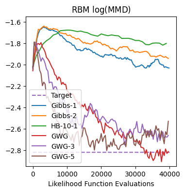
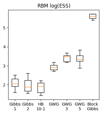
Figure 9: RBM Sampling with Gibbs-With-Gradients extensions. GWG-3 and GWG-5 are the multi-sample variant of GWG described above with $n=3$ and $n=5$, respectively.

Appendix E Restricted Boltzmann Machines

Restricted Boltzmann Machines define a distribution over binary data $x$ and latent variables $h$. The model is defined as:

$$\log p(x,h)=h^{T}Wx+b^{T}x+c^{T}h-\log Z$$ (28)

where $Z$ is the normalizing constant and $\{W,b,c\}$ are the model’s parameters. In this model we can efficiently marginalize out the latent variable $h$ to obtain:

$$\log p(x) =\log\sum_{h}p(x,h)$$

$$=\log\sum_{h}\exp(h^{T}Wx+b^{T}x+c^{T}h)$$

$$=\log(1+\exp(Wx+c))+b^{T}x-\log Z$$ (29)

While the joint and marginal are both unnormalized, we can see the conditional distirbutions can be easily normalized and take the form:

$$p(x|h) =\text{Bernoulli}(Wx+c)$$

$$p(h|x) =\text{Bernoulli}(W^{T}h+b).$$

We can exploit this structure to more efficiently sample from RBMs. We can perform Block-Gibbs updates by starting at some initial $x$, and repeatedly sample $h\sim p(h|x)$, ${x\sim p(x|h)}$. Exploiting this structure leads to much more efficient sampling than standard Gibbs and other samplers (see Figure 3).

E.1 Experimental Details

We explore the performance of various approaches to sample from an RBM trained on the MNIST dataset. The RBM has 500 hidden units (and 784 visible units). We train the model using contrastive divergence (Hinton, 2002) for 1 epoch through the dataset using a batch size of 100. We use 10 steps of MCMC sampling using the Block-Gibbs sampler defined above to generate samples for each training iteration. We use the Adam (Kingma & Ba, 2014) optimizer with a learning rate of $.001$.

Our first result compares samples generated by various approaches with samples generated with the Block-Gibbs sampler described above. We generate a set of 500 samples using the Block-Gibbs sampler run for 10,000 steps. At this length, the samples are very close to true samples from the model. Next we generate a set of 100 samples from a number of other samplers: Gibbs, Hamming Ball and Gibbs-With-Gradients. After every MCMC transition we compute the Kernelized Maximum Mean Discrepancy (Gretton et al., 2012) between the current set of samples and our “ground-truth” long-run Block-Gibbs samples. We use an exponential average Hamming kernel $K(x,x^{\prime})=\exp\left(-\sum_{i=1}^{D}\frac{\mathbf{1}(x_{i}=x^{\prime}_{i})}{D}\right)$ to compute the MMD.

The next result is the effective sample size of a test statistic for each sampler. Following Zanella (2020), our test statistic is the Hamming distance between the current sample and a random input configuration. We present a box-plot showing the median, standard-deviation, and outliers over 32 chains.

E.2 Additional Results

We visualize the samples after 10,000 steps of each tested sampler in Figure 10. We can see the Gibbs-With-Gradients samples much more closely matches the Block-Gibbs samples. This result is reflected in the improved MMD scores see in Figure 3 (left).

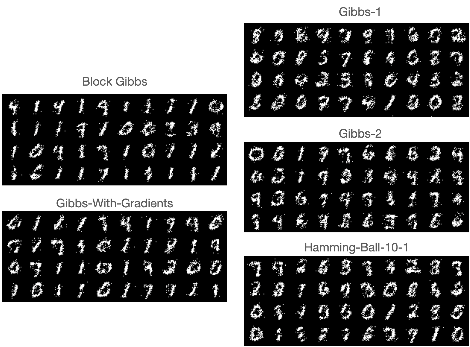
Figure 10: Sets of samples drawn from a fixed RBM with various MCMC approaches after 10,000 steps.

Appendix F Ising Models

Ising models are unnormalized models for binary data defined as

$$\log p(x)=x^{T}Jx+b^{T}x-\log Z$$ (30)

where $J$ and $b$ are the model’s parameters and $Z$ is the normalizing constant. $J$ determines which other variables each $x_{i}$ is correlated with. If $J=0$ then the model becomes a factorized Bernoulli distribution. If all of the non-zero indices of $J$ are the same, then we can pull out this value and rewrite the model as

$$\log p(x)=\theta x^{T}Jx+b^{T}x-\log Z$$ (31)

where now $\theta$ controls how correlated each $x_{i}$ is with its connected variables and $J$ controls which variables each $x_{i}$ is connected to. Our lattice Ising models take this form where the $J$ is the adjacency matrix of a cyclic 2D lattice and $\theta$ controls the strength of the connectivity.

F.1 Experimental Details: Sampling

We experiment with our sampler’s ability to sample from Ising models on the 2D cyclic lattice as various factors chage. These include the connectivity strength and the size of the lattice. We run each sampler for 100,000 steps and evaluate using the ESS of a test statistic. Following Zanella (2020) our test statistic is the Hamming distance between the current sample and a random input configuration. We present the ESS (in log-scale), averaged with standard-errors, over 32 random seeds.

We can see in both 10x10 and 40x40 lattice sizes, our sampler outperforms Gibbs and the Hamming ball.

F.2 Experimental Details: Training

We create Ising models with 2 kinds of graph structure; a cyclic 2D lattice and a random Erdos-Renyi (ER) graph. For the lattice we create models with a 10x10, 25x25, and 40x40 lattice leading to 100, 625, and 1600 dimensional distributions. We train models with connectivity $\theta\in[-.1,0.0,.1,.25,.5]$.

For the ER graph, we create a model with 200 nodes. The ER edge probability is chosen so each node has an average of 4 neighbors. The strength of each edge is IID sampled from $N\left(0,\frac{1}{4}\right)$.

A dataset of 2000 examples is generated from each model using 1,000,000 steps of Gibbs sampling. We train models using persistent contrastive divergence (Tieleman, 2008) with a buffer size of 256 examples. Models are trained with the Adam optimizer (Kingma & Ba, 2014) using a learning rate of .001 and a batch size of 256. We update the persistent samples using Gibbs and Gibbs-With-Gradients. We train models with $\{5,10,25,50,100\}$ steps of MCMC per training iteration and compare their results. We train all models with an $\ell 1$ penalty to encourage sparsity with strength .01.

We compare results using the root-mean-squared-error between the true connectivity matrix $J$ and the inferred connectivity matrix $\hat{J}$.

F.3 Additional Results: Training Ising Models

In Figure 11, we present an expanded version of Figure 6 which presents additional results. In these additional experiments we find Gibbs-With-Gradients considerably outperforms training with Gibbs sampling.

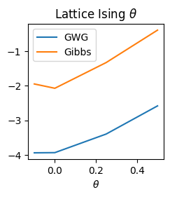
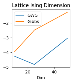
Figure 11: Training Ising models. Top Left: Lattice Ising with increasing $\theta$ (dim = 50, steps = 50). Top Right: Lattice Ising with increasing dimension ($\theta=.25$, steps = 25). Bottom Right: Lattice Ising with increasing steps (dim = 25, $\theta=.25$). Bottom Right: Erdos-Renyi Ising with increasing steps. Values are $\log$(RMSE) between the learned $J$ and the true $J$. Gibbs-With-Gradients leads to better solutions with lower computational cost.

Appendix G Factorial Hidden Markov Models

Factorial Hidden Markov Models (FHMM) are a generalization of Hidden Markov Models and model real-valued time-series data. The observed data $y\in R^{L}$ is generated conditioned on a discrete latent-variable $x\in\{0,1\}^{L\times K}$. This latent-variable is drawn from the product of $K$ independent Markov processes as seen below. The data $y_{t}$ is generated by by the $K$-dimensional state vector $x_{t}$ with Gaussian noise added.

$$p(x,y) =p(y|x)p(x)$$

$$p(y|x) =\prod_{t=1}^{L}\mathcal{N}(y_{t};Wx_{t}+b,\sigma^{2})$$

$$p(x) =p(x_{1})\prod_{t=2}^{L}p(x_{t}|x_{t-1})$$

$$p(x_{1}) =\prod_{k=1}^{K}\text{Bernoulli}(x_{1k};\alpha_{k})$$

$$p(x_{t+1}|x_{t}) =\prod_{k=1}^{K}\text{Bernoulli}(x_{(t+1)k};\beta_{k}^{x_{tk}}(1-\beta_{k})^{1-x_{tk}})$$ (32)

The posterior $p(x|y)$ has no closed form and thus we must rely on MCMC techniques to sample from it.

G.1 Experimental Details

We sample the parameters of an FHMM randomly as

$$W,b \sim\mathcal{N}(0,I)$$ (33)

and set $\sigma^{2}=.5$, $\alpha_{k}=.1$ and $\beta_{k}=.95$ for for all $k$.

We then sample $x\sim p(x)$ and $y\sim p(y|x)$ and run all samplers for 10,000 steps to generate samples from $p(x|y)$. The Hamming Ball Sampler (Titsias & Yau, 2017) is special for this model as it exploits the known block-structure of the posterior. We use a block size of 10 and the blocks are chosen to be all 10 dims of the latent state at a randomly chosen time $x_{t}$. Thus, this sampler is aware of more hard-coded structure in the model than the Gibbs baseline and Gibbs-With-Gradients.

Appendix H Potts Models for Proteins

We train the MCMC models using PCD (Tieleman, 2008) with a buffer size of 2560. At each training iteration we sample a mini batch of 256 examples and 256 random samples from the persistent sample buffer. These are updated using 50 steps of either Gibbs or Gibbs-With-Gradients and the gradient estimator of Equation 12 is used to update the model parameters. We train for 10,000 iterations using the Adam optimizer (Kingma & Ba, 2014). Following Marks et al. (2011) we use block-$\ell 1$ regularization. This regularizer takes the form

$$\mathcal{L}_{1}(J)=\sum_{ij}||J_{ij}||_{2}.$$ (34)

We add this regularizer to the maximum likelihood gradient estimator. We tested regularization strength parameters in $\{.1,.03,.01\}$ and found $.01$ to work best for PLM, Gibbs, and Gibbs-With-Gradients.

Ground truth couplings were extracted from an experimentally validated distance-map. As is standard, we consider any pair of amino acids to be a contact if they are within 5 angstroms of each other.

H.1 Recall on PF10018

We do not present results on PF10018 in the main body as it was used to tune hyper-parameters. For completeness, we present them here in Figure 12. As with the other protiens, the MCMC-based training outperforms PLM but by a smaller margin and GWG and Gibbs perform comparably here. This further supports the benefit of MCMC training over PLM sets in on larger data as does the benefit of GWG over Gibbs.

Figure 12: Recall Curves for contact prediction with Potts models.

H.2 Visualized Contacts

We visualize the inferred couplings for CADH1_HUMAN in Figure 13. We see that GWG most accurately matches the known structure with Gibbs inferring spurious couplings and PLM missing many couplings near the diagonal.

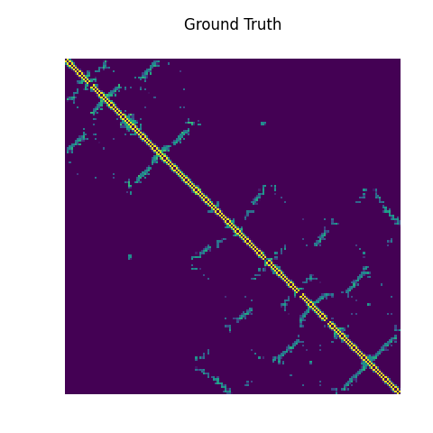
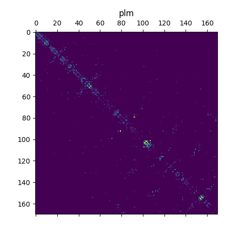
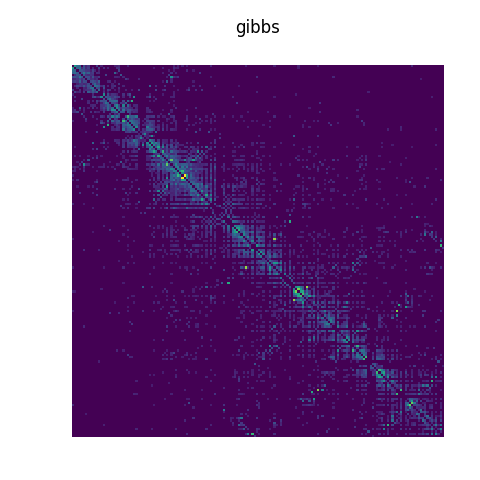
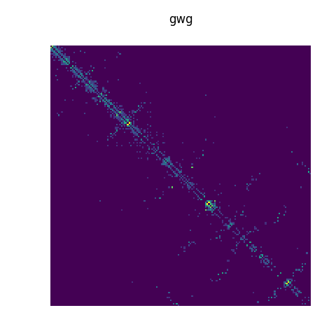
Figure 13: Inferred Couplings for CADH1_HUMAN. “Ground Truth” is the matrix of known distances between amino acids. All other matrices are the norms of the Potts model $J_{ij}$ parameter.

Appendix I Deep EBMs

I.1 Architectures

We train on two types of data; binary and categorical. For the binary datasets, the data is represented as $\{0,1\}^{D}$ where $D$ is the dimension of the data.

For the categorical datasets, each categorical variable is represented as a “one-hot” vector. Thus, for image data, each pixel is represented with a 256-dimensional vector. To deal with the very high dimensionality of this input parameterization, we first map each one-hot vector to a learned, low-dimensional embedding with a linear transformation. We map to $D_{p}=4$ dimensions for all models tested. We then feed this $(D\times D_{p})$-dimensional input to our network. There are certainly more efficient ways to represent this data, but our intention was not to achieve state-of-the-art results on these datasets and instead to demonstrate our sampler could enable the training of energy-based models on high-dimensional discrete data, so we use the most straight-forward parameterization.

The ResNet used for our EBM is identical for all datasets. The network has 8 residual blocks with 64 feature maps. Each residual block has 2 convolutional layers. The first two residual blocks have a stride of 2. The output features are mean-pooled across the spatial dimensions and a single linear layer is used on top to provide the energy. The Swish (Ramachandran et al., 2017) nonlinearity ($x\cdot\sigma(x)$) is used throughout.

I.2 Experimental Details

We trained all models Adam (Kingma & Ba, 2014) using a learning rate of $0.0001$. We linearly warm-up the learning rate for the first 10,000 iterations. We found this was necessary to help burn in the replay buffer of samples.

For the large datasets (static/dynamic MNIST, Omniglot) we use a replay buffer with 10,000 samples. For the smaller datasets (Caltech, Freyfaces, Histopathology) the buffer size is 1000. Unlike recent work on continuous EBMs (Du & Mordatch, 2019; Grathwohl et al., 2019), we do not reinitialize the buffer samples to noise. We found this resulted in unstable training and lower likelihoods.

We train all models for 50,000 iterations. We use the same training/validation/testing splits as Tomczak & Welling (2018). We evaluate models every 5000 iterations using 10,000 steps of AIS. We select the model which performs the best on the validation data under this procedure. Final results in Table 2 are generated from the selected models by running 300,000 iterations of AIS. We evaluate using a model who’s weights are given by an exponential moving average of the training model’s weights. This is analogous to training with “fast-weights” as in Tieleman & Hinton (2009). We find this greatly improves likelihood performance and sample quality. We use an exponential moving average with weight $0.999$ and did not experiment with other values.

We believe better results could be obtained with larger models or alternative architectures, but we leave this for future work.

I.2.1 Partition Function Estimation with AIS

We estimate likelihoods by estimating the partition function using Annealed Importance Sampling (AIS) (Neal, 2001). AIS underestimates the log-partition-function leading to over-estimating the likelihood. The estimation error can be reduced by using a larger number of intermediate distributions or a more efficient MCMC sampler. Results presented in Table 2 were generated with 300,000 intermediate distributions. We chose this number as it appears to be sufficiently high for our partition function estimate to converge. Despite this, these are upper-bounds and therefore should not be considered definitive proof that one model achieves higher likelihoods than another.

We anneal between our model’s unnormalized log-probability $f(x)$ and a multivariate Bernoulli or Categorical distribution, $\log p_{n}(x)$, fit to the training data, for binary and categorical data, respectively.

$$f_{t}(x)=\beta_{t}f(x)+(1-\beta_{t})\log p_{n}(x)$$ (35)

where $\beta_{t}$ is linearly annealed from 0 to 1. Alternative strategies such as sigmoid annealing could be used, but we leave this for future work.

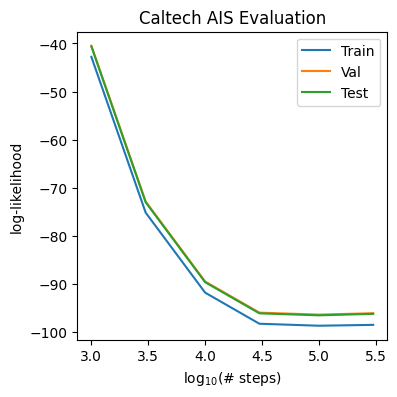
Figure 14: AIS likelihood estimates as the number of intermediate distributions increases for our Caltech Silhouettes Resnet EBM. Values converge after $30,000\approx 10^{4.5}$ step s

In Figure 14 we plot the estimated likleihoods for our Caltech Silhouettes models as the number of intermediate distributions increases. It can be seen that between 30,000 and 300,000 ($\approx 10^{4.5}\rightarrow 10^{5.5}$) the values appear to be converged, thus we feel our reported number faithfully represent our models’ performance.

I.3 Additional Results

We present additional long-run samples from our convolutional EBM. These samples were generated using an annealed Markov Chain (as described above) and Gibbs-With-Gradients as the base MCMC sampler.

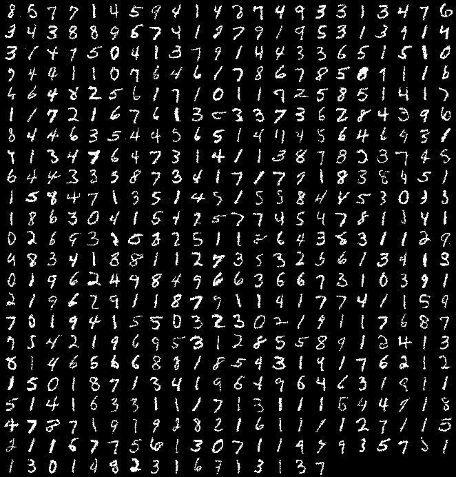
Figure 15: Static MNIST Samples

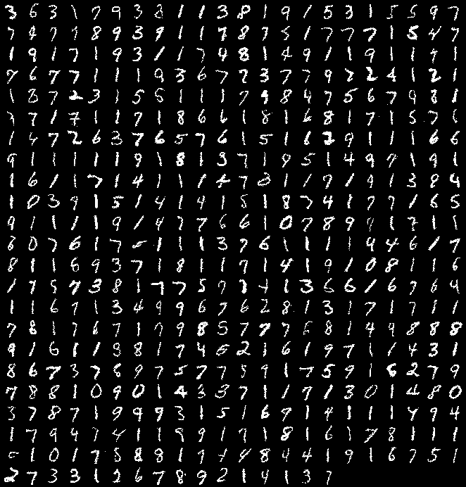
Figure 16: Dynamic MNIST Samples

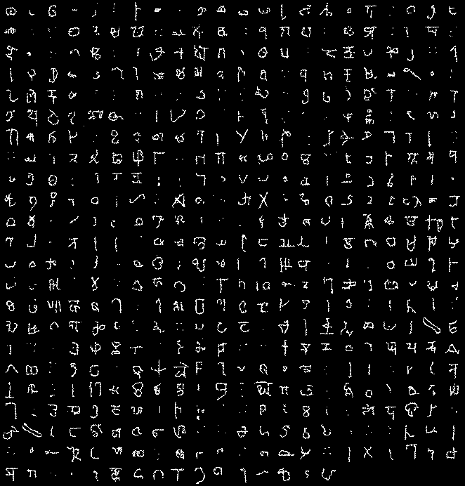
Figure 17: Omniglot Samples

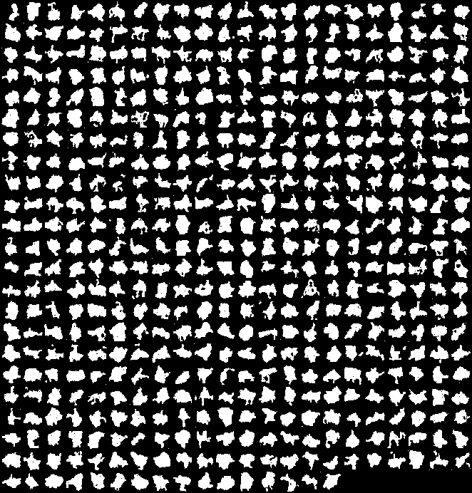
Figure 18: Caltech Silhouette Samples

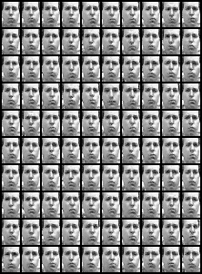
Figure 19: Freyfaces Samples

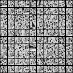
Figure 20: Histopathology Samples

Appendix J Preliminary Text EBM Results

There has recently been interest in learning Energy-Based Models of text data. An EBM for text could enable non-autoregressive generation and more flexible conditioning than autoregressive models. For example, an EBM trained on language pairs $p(x,y)$ could be used to translate in either direction without retraining and could be structured as $\log p(x,y)=f_{\theta}(x)^{T}g_{\phi}(y)-\log Z$ so that each language component could be trained separately. We also have much more architectural freedom when specifying EBMs meaning $f_{\theta}$ is free to be a CNN, RNN, transformer, or MLP.

A few works have had success training and applying text EBMs. Deng et al. (2020) find that EBMs can be used to improve the generative modeling performance of large-scale transformer language models and He et al. (2021) find that Joint Energy-Based Models (Grathwohl et al., 2019) can improve the calibration of text classifiers. Because of the discrete structure of the text data, both of these works train using Noise Contrastive Estimation (Gutmann & Hyvärinen, 2010) using a pretrained autoregressive language model as the noise distribution. NCE requires a noise distribution which can be sampled from and enables exact likelihood computation. Thus, these approaches rely on and are limited by the quality of these autoregressive models.

Ideally, we could train a text EBM on its own, without an auxiliary model. One way to do this is to use the gradient estimator of Equation 12 but the MCMC sampling task is very challenging. Text models typically have a vocabulary above 10,000 words so the size of the discrete sample space is tremendous. Further, as noted in Section 8, to apply Gibbs sampling to a model like this we would need to evaluate the energy function over 10,000 times to perform a single step of sampling!

We believe Gibbs-With-Gradients can provide an avenue to train and sample from these kinds of models. As a preliminary experiment we train non-autoregressvive language models on a shortened version of the Penn Tree Bank dataset (Taylor et al., 2003). This is a dataset of short sentences with 10,000 words. We cut out all sentences with greater than 20 words and pad all shorter sentences with an “end of sequence” token. We feel this simplified setting is sufficient for a proof-of-concept as the configuration space is very large and Gibbs sampling is not feasible.

Our model consists of a bidirectional LSTM (Gers et al., 1999) with 512 hidden units. We project the 10,000 words to an embedding of size 256 with a learned mapping. To compute the energy, we take the last hidden-state from each direction, concatenate them together to a 1024-dimensional vector. We project this to 512 dimensions with a linear layer, apply a Swish nonlinearity and then map to 1 dimension with another linear layer.

We train using PCD with a buffer size of 1000 and we use 20 steps of MCMC with Gibbs-With-Gradients to update the samples at every training iteration. Besides this, training was identical to our image EBMs in section 8.

We compare with a simple autoregressive language model which is based on an LSTM with 512 hidden units and use a learned word embedding of size 256.

We find the autoregressive model slightly outperforms the EBM. The test-set log-likelihoods of the EBM and autoregressive model are $-77.16$ and $-74.0$, respectively. For comparison, a uniform distribution over possible tokens obtains $-184.21$ and a Categorical distribution fit to the training data obtains $-100.05$.

While we are aware these are far from state-of-the-art language modelling results, we believe they demonstrate that Gibbs-With-Gradients can enable MCMC-trained EBMs to successfully model text data with large vocabulary sizes. At every step, the sampler has $10,000\times 20=200,000$ choices for possible updates. Despite this massive sampling space, we find our acceptance rates during training are just above 70% making our approach at least 3500 times more efficient than Gibbs sampling.

We believe improvements could be obtained through larger models and more tuning. To further scale this approach, we believe we will need to develop further approximations which make sampling from very large categorical distributions more efficient and numerically stable. We leave this for future work.

References

- Besag (1975) Besag, J. Statistical analysis of non-lattice data. Journal of the Royal Statistical Society: Series D (The Statistician), 24(3):179–195, 1975.
- Besag (1994) Besag, J. Comments on “representations of knowledge in complex systems” by u. grenander and mi miller. J. Roy. Statist. Soc. Ser. B, 56:591–592, 1994.
- Burda et al. (2015) Burda, Y., Grosse, R., and Salakhutdinov, R. Accurate and conservative estimates of mrf log-likelihood using reverse annealing. In Artificial Intelligence and Statistics, pp. 102–110, 2015.
- Deng et al. (2020) Deng, Y., Bakhtin, A., Ott, M., Szlam, A., and Ranzato, M. Residual energy-based models for text generation. arXiv preprint arXiv:2004.11714, 2020.
- Du & Mordatch (2019) Du, Y. and Mordatch, I. Implicit generation and generalization in energy-based models. arXiv preprint arXiv:1903.08689, 2019.
- Gers et al. (1999) Gers, F. A., Schmidhuber, J., and Cummins, F. Learning to forget: Continual prediction with lstm. 1999.
- Grathwohl et al. (2019) Grathwohl, W., Wang, K.-C., Jacobsen, J.-H., Duvenaud, D., Norouzi, M., and Swersky, K. Your classifier is secretly an energy based model and you should treat it like one. arXiv preprint arXiv:1912.03263, 2019.
- Grathwohl et al. (2020a) Grathwohl, W., Kelly, J., Hashemi, M., Norouzi, M., Swersky, K., and Duvenaud, D. No mcmc for me: Amortized sampling for fast and stable training of energy-based models. arXiv preprint arXiv:2010.04230, 2020a.
- Grathwohl et al. (2020b) Grathwohl, W., Wang, K.-C., Jacobsen, J.-H., Duvenaud, D., and Zemel, R. Learning the stein discrepancy for training and evaluating energy-based models without sampling. In International Conference on Machine Learning, pp. 3732–3747. PMLR, 2020b.
- Gretton et al. (2012) Gretton, A., Borgwardt, K. M., Rasch, M. J., Schölkopf, B., and Smola, A. A kernel two-sample test. The Journal of Machine Learning Research, 13(1):723–773, 2012.
- Gutmann & Hyvärinen (2010) Gutmann, M. and Hyvärinen, A. Noise-contrastive estimation: A new estimation principle for unnormalized statistical models. In Proceedings of the Thirteenth International Conference on Artificial Intelligence and Statistics, pp. 297–304. JMLR Workshop and Conference Proceedings, 2010.
- Han & Liu (2018) Han, J. and Liu, Q. Stein variational gradient descent without gradient. arXiv preprint arXiv:1806.02775, 2018.
- Han et al. (2020) Han, J., Ding, F., Liu, X., Torresani, L., Peng, J., and Liu, Q. Stein variational inference for discrete distributions. arXiv preprint arXiv:2003.00605, 2020.
- He et al. (2016) He, K., Zhang, X., Ren, S., and Sun, J. Deep residual learning for image recognition. In Proceedings of the IEEE conference on computer vision and pattern recognition, pp. 770–778, 2016.
- He et al. (2021) He, T., McCann, B., Xiong, C., and Hosseini-Asl, E. Joint energy-based model training for better calibrated natural language understanding models. arXiv preprint arXiv:2101.06829, 2021.
- Hill et al. (2020) Hill, M., Mitchell, J., and Zhu, S.-C. Stochastic security: Adversarial defense using long-run dynamics of energy-based models. arXiv preprint arXiv:2005.13525, 2020.
- Hinton (2002) Hinton, G. E. Training products of experts by minimizing contrastive divergence. Neural computation, 14(8):1771–1800, 2002.
- Hinton (2009) Hinton, G. E. Deep belief networks. Scholarpedia, 4(5):5947, 2009.
- Ingraham & Marks (2017) Ingraham, J. and Marks, D. Variational inference for sparse and undirected models. In International Conference on Machine Learning, pp. 1607–1616. PMLR, 2017.
- Ising (1924) Ising, E. Beitrag zur Theorie des Ferround Paramagnetismus. PhD thesis, PhD thesis (Mathematisch-Naturwissenschaftliche Fakultät der Hamburgischen …, 1924.
- Kingma & Ba (2014) Kingma, D. P. and Ba, J. Adam: A method for stochastic optimization. arXiv preprint arXiv:1412.6980, 2014.
- Kingma & Welling (2013) Kingma, D. P. and Welling, M. Auto-encoding variational bayes. arXiv preprint arXiv:1312.6114, 2013.
- Lapedes et al. (1999) Lapedes, A. S., Giraud, B. G., Liu, L., and Stormo, G. D. Correlated mutations in models of protein sequences: phylogenetic and structural effects. Lecture Notes-Monograph Series, pp. 236–256, 1999.
- Łatuszyński et al. (2013) Łatuszyński, K., Roberts, G. O., Rosenthal, J. S., et al. Adaptive gibbs samplers and related mcmc methods. The Annals of Applied Probability, 23(1):66–98, 2013.
- Levin & Peres (2017) Levin, D. A. and Peres, Y. Markov chains and mixing times, volume 107. American Mathematical Soc., 2017.
- Liu (1996) Liu, J. S. Peskun’s theorem and a modified discrete-state gibbs sampler. Biometrika, 83(3), 1996.
- Liu & Wang (2016) Liu, Q. and Wang, D. Stein variational gradient descent: A general purpose bayesian inference algorithm. Advances in neural information processing systems, 29:2378–2386, 2016.
- Lyu (2012) Lyu, S. Interpretation and generalization of score matching. arXiv preprint arXiv:1205.2629, 2012.
- Maddison et al. (2016) Maddison, C. J., Mnih, A., and Teh, Y. W. The concrete distribution: A continuous relaxation of discrete random variables. arXiv preprint arXiv:1611.00712, 2016.
- Marks et al. (2011) Marks, D. S., Colwell, L. J., Sheridan, R., Hopf, T. A., Pagnani, A., Zecchina, R., and Sander, C. Protein 3d structure computed from evolutionary sequence variation. PloS one, 6(12):e28766, 2011.
- Neal (2001) Neal, R. M. Annealed importance sampling. Statistics and computing, 11(2):125–139, 2001.
- Neal et al. (2011) Neal, R. M. et al. Mcmc using hamiltonian dynamics. Handbook of markov chain monte carlo, 2(11):2, 2011.
- Nijkamp et al. (2020) Nijkamp, E., Hill, M., Han, T., Zhu, S.-C., and Wu, Y. N. On the anatomy of mcmc-based maximum likelihood learning of energy-based models. In Proceedings of the AAAI Conference on Artificial Intelligence, volume 34, pp. 5272–5280, 2020.
- Nishimura et al. (2017) Nishimura, A., Dunson, D., and Lu, J. Discontinuous hamiltonian monte carlo for sampling discrete parameters. arXiv preprint arXiv:1705.08510, 2, 2017.
- Ramachandran et al. (2017) Ramachandran, P., Zoph, B., and Le, Q. V. Searching for activation functions. arXiv preprint arXiv:1710.05941, 2017.
- Richardson et al. (2010) Richardson, S., Bottolo, L., and Rosenthal, J. S. Bayesian models for sparse regression analysis of high dimensional data. Bayesian Statistics, 9:539–569, 2010.
- Song & Ermon (2019) Song, Y. and Ermon, S. Generative modeling by estimating gradients of the data distribution. In Advances in Neural Information Processing Systems, pp. 11918–11930, 2019.
- Song & Ou (2018) Song, Y. and Ou, Z. Learning neural random fields with inclusive auxiliary generators. arXiv preprint arXiv:1806.00271, 2018.
- Taylor et al. (2003) Taylor, A., Marcus, M., and Santorini, B. The penn treebank: an overview. Treebanks, pp. 5–22, 2003.
- Tieleman (2008) Tieleman, T. Training restricted boltzmann machines using approximations to the likelihood gradient. In Proceedings of the 25th international conference on Machine learning, pp. 1064–1071, 2008.
- Tieleman & Hinton (2009) Tieleman, T. and Hinton, G. Using fast weights to improve persistent contrastive divergence. In Proceedings of the 26th Annual International Conference on Machine Learning, pp. 1033–1040, 2009.
- Titsias & Yau (2017) Titsias, M. K. and Yau, C. The hamming ball sampler. Journal of the American Statistical Association, 112(520):1598–1611, 2017.
- Tomczak & Welling (2018) Tomczak, J. and Welling, M. Vae with a vampprior. In International Conference on Artificial Intelligence and Statistics, pp. 1214–1223. PMLR, 2018.
- Umrigar (1993) Umrigar, C. J. Accelerated metropolis method. Phys. Rev. Lett., 71:408–411, Jul 1993. doi: 10.1103/PhysRevLett.71.408. URL https://link.aps.org/doi/10.1103/PhysRevLett.71.408.
- Zanella (2020) Zanella, G. Informed proposals for local mcmc in discrete spaces. Journal of the American Statistical Association, 115(530):852–865, 2020.