Confinement-Deconfinement transition and $Z_{2}$ symmetry in $Z_{2}+$Higgs theory

Abstract

We study the Polyakov loop and the $Z_{2}$ symmetry in the lattice $Z_{2}+$Higgs theory in four dimensional space using Monte Carlo simulations. The results show that this symmetry is realised in the Higgs symmetric phase for large number of “temporal” lattice sites. To understand this dependence on the number of “temporal” sites, we consider a one dimensional model by keeping terms of the original action corresponding to a single spatial site. In this approximation the partition function can be calculated exactly as a function of the Polyakov loop. The resulting free energy is found to have the $Z_{2}$ symmetry in the limit of large temporal sites. We argue that this is due to $Z_{2}$ invariance as well as dominance of the distribution or density of states corresponding to the action.

I Introduction

$Z_{N}$ symmetry plays an important role in the confinement-deconfinement (CD) transition in pure $SU(N)$ gauge theories tHooft:1977nqb ; McLerran:1981pb ; Belyaev:1991gh . In these theories, at finite temperature, the allowed gauge transformations are classified by the centre of the gauge group, i.e $Z_{N}$. Under these $Z_{N}$ gauge transformations, i.e $Z_{N}$ symmetry, the Polyakov loop ($L$) transforms like magnetisation, in spin models Kogut:1979wt . In the confinement and deconfinement phases the Polyakov loop acquires vanishing and non-zero thermal average values respectively, hence plays the role of an order parameter for the confinement-deconfinement (CD) transition, Kuti:1980gh ; McLerran:1980pk ; Weiss:1980rj ; Creutz:1980zw ; Svetitsky:1982gs . In the deconfined phase, the $Z_{N}$ symmetry is spontaneously broken which leads to $N$-degenerate states Yaffe:1982qf ; Svetitsky:1985ye ; Celik:1983wz .

The $Z_{N}$ symmetry of pure $SU(N)$ gauge theory is spoiled when matter fields are included. Gauge transformations which are not periodic in temporal directions can not act on the matter fields. These may act only on the gauge fields but in the process the action does not remain invariant. There are many studies on the effect of matter fields on this symmetry. Perturbative loop calculations of the Polyakov loop effective potential show that this symmetry is explicitly broken by matter fields in the fundamental representation  Weiss:1981ev ; Belyaev:1991np ; Guo:2018scp . The mean-field approximations of lattice partition functions in the strong coupling limit also show the explicit breaking of the $Z_{N}$ symmetry Green:1983sd ; Karsch:2000zv . On the other hand, non-perturbative studies of $CD$ transition in $2-$colour QCD show a sharp transition suggesting small explicit breaking of $Z_{2}$ symmetry Satz:1985js .

Recent non-perturbative Monte Carlo simulations of $SU(2)+$Higgs theory show that the strength of $Z_{2}$ explicit breaking depends on the Higgs condensate Biswal:2015rul . These studies find that the $CD$ transition exhibits critical behaviour in the Higgs symmetric phase for large number of temporal sites ($N_{\tau}$) Biswal:2015rul . The distributions of the Polyakov loop are found to be $Z_{2}$ symmetric, albeit within statistical errors, suggesting the realisation of $Z_{2}$ symmetry in the Higgs symmetric phase. In reference Biswal:2016xyq , it was argued that the emergence of $Z_{2}$ symmetry is due to enhancement of the configuration/ensemble space with $N_{\tau}$. This enhancement makes it possible that the change in the Euclidean action due to $Z_{2}$ “rotation” of gauge links can be compensated by changing the Higgs field appropriately. This was numerically tested by updating the Higgs field using Monte Carlo steps after $Z_{2}$ rotating the gauge fields.

The non-invariance of the action under $Z_{2}$ gauge transformation which are not periodic in temporal directions does not necessarily imply the explicit breaking of $Z_{2}$ symmetry. The presence of $Z_{2}$ symmetry or it’s explicit breaking can only be inferred from the free energy of the Polyakov loop. In the free energy or the partition function calculations, two factors play important roles. They are the distribution of the action, which is also known as the density of states ($DoS$) and the Boltzmann factor. The latter clearly does not respect the $Z_{2}$ symmetry. So the realisation of the $Z_{2}$ symmetry must come from the $DoS$ and it’s dominance over the Boltzmann factor. Computing the $DoS$ in $SU(N)+$Higgs theory is a difficult task as the configuration space is infinite. In this situation, the $Z_{2}+$Higgs theory in four dimensions provides a suitable alternative. Since the field variables take values $\pm 1$, it is possible to calculate the $DoS$ with some simplifications.

The $Z_{2}+$Higgs theory has been extensively studied in literature Balian:1974ts ; Balian:1974xw ; Creutz:1979he ; Fradkin:1978dv ; Callaway:1981rt ; Bhanot:1981ug ; Bhanot:1980ga . The phase diagram of this theory is found to be similar to that of $SU(N)+$Higgs theories in $3$ and $4-$dimensions  Jongeward:1980wx ; Creutz:1983ev . Though, in this theory there is no analog of the beta-functions of $SU(N)+$Higgs theories and the temperature is controlled by the couplings of the therory Caselle:1995wn . The similarity with the $SU(N)+$Higgs theories arises when periodic/anti-periodic boundary condition is imposed on the Higgs field, in any one of the four dimensions. As a consequence gauge transformations which are not periodic in this “temporal” direction are not allowed and the $Z_{2}$ symmetry is explicitly broken similar to the explicit breaking of $Z_{N}$ symmetry in $SU(N)+$Higgs theories. It is important to note the difference on the role of $N_{\tau}$ between $Z_{2}+$Higgs and $SU(N)+$Higgs theories. Though in both cases increase in $N_{\tau}$ introduces additional degrees of freedom, in $SU(N)+$Higgs theory to study $Z_{N}$ symmetry at fixed temperature the couplings need to be tuned.

In this paper, the $Z_{2}$ symmetry of the Polyakov loop and the nature of $CD$ transition are studied by varying the number of lattice points, $N_{\tau}$, along the temporal direction. The computations are mostly done on the Higgs symmetric side of the Higgs transition line. Our results show that the $Z_{2}$ symmetry is realised for large $N_{\tau}$. Also the behaviour of the $CD$ transition is found to be similar to the pure gauge case apart from the location of the critical point. To understand the role of $N_{\tau}$ a $0+1$ dimensional model is considered by keeping temporal component of the gauge Higgs interaction corresponding to a single spatial coordinate. The reason for this choice is the fact that only the temporal component of the gauge Higgs interaction is sensitive to the $Z_{2}$ gauge transformations. For the one dimensional model the Polyakov loop can take values $\pm 1$. For each of these cases the free energy can be calculated exactly. The free energy calculations show the emergence of $Z_{2}$ symmetry in the large $N_{\tau}$ limit for arbitrary interaction coupling. Further the Monte Carlo results for the distribution of the interaction term is reproduced well by $0+1$ dimensional $DoS$ with a simple Boltzmann factor, though with a different value of the coupling strength. The $DoS$ for both values of the Polyakov loop is sharply peaked at zero. $Z_{2}$ symmetry is clearly observed near the peak, the differences appear when the action takes the limiting values. Since the peak height grows with $N_{\tau}$, the $DoS$ will dominate the thermodynamics in the $N_{\tau}\to\infty$, leading to vanishingly small $Z_{2}$ explicit symmetry breaking.

This paper is organised as follows. In section II, we discuss the $Z_{2}$ symmetry in $Z_{2}+$Higgs theory. This is followed by numerical simulations of $CD$ transition and the $Z_{2}$ symmetry in pure gauge theory and in the presence of Higgs in section III. In section IV, we derive the free energy of the Polyakov loop in a $0+1$ dimensional model, and relate the results to $4-$dimensional Monte Carlo simulations. In section V, discussions and conclusions are presented.

II $Z_{2}$ symmetry in $Z_{2}+$Higgs gauge theory.

The action for the $Z_{2}+$Higgs theory in four dimensional lattice $(N_{s}^{3}\times N_{\tau})$ is given by,

$$S=-\beta_{g}\sum_{P}U_{P}-\kappa\sum_{{n},\hat{\mu}}\Phi_{{n}+\hat{\mu}}U_{n,\hat{\mu}}\Phi_{n}.$$ (1)

Here $n=(n_{1},n_{2},n_{3},n_{4})$ represents a point on the lattice with $1\leq n_{1},n_{2},n_{3}\leq N_{s}$ and $1\leq n_{4}\leq N_{\tau}$. As mentioned above we assume that the fourth direction is the temporal direction. $U_{n,\hat{\mu}}$ represents the gauge links in $\hat{\mu}$ direction between the lattice point $n$ and $n+\hat{\mu}$. The Higgs field $\Phi_{n}$ lives at the site $n$. Both $U_{n,\hat{\mu}}$ and $\Phi_{n}$ take values $\pm 1$. $\beta_{g}$ is the gauge coupling and $\kappa$ is the gauge Higgs interaction strength. Figure. 1 shows a schematic layout of the gauge links and Higgs variable on the lattice.

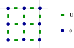
Figure 1: Position of gauge links U and Higgs fields $\Phi$ on lattice

The plaquette $U_{P}$ which is path ordered product of the links along an elementary square on the $\mu-\nu$ plane, i.e

$$U_{P}=U_{n,\hat{\mu}}U_{n+\hat{\mu},\hat{\nu}}U_{n+\hat{\nu},\hat{\mu}}U_{n,\hat{\nu}}.$$ (2)

Figure. 2 shows the sketch of an elementary plaquette.

Figure 2: Sketch of an elementary plaquette $U_{P}$

The pure gauge part of the action, first term in Eq.1, is invariant under the $Z_{2}$ gauge transformations,

$$U_{n,\hat{\mu}}\rightarrow V_{n}U_{n,\hat{\mu}}V^{-1}_{n+\hat{\mu}}$$ (3)

where $V_{n}=\pm 1\in Z_{2}$. The $V_{n}$’s satisfy the following boundary condition,

$$V(\vec{n},n_{4}=1)=zV(\vec{n},n_{4}=N_{\tau}).$$ (4)

$z=\pm 1\in Z_{2}$. So the gauge transformations can be classified by the group $Z_{2}$. For $z=-1$ the gauge transformations are anti-periodic in the temporal direction.

The Polyakov loop, which is defined as the product of links along the temporal direction, i.e,

$$L(\vec{n})=\displaystyle\prod_{n_{4}=1}^{N_{\tau}}U_{{(\vec{n},n_{4})},\hat{4}}$$ (5)

transforms non-trivially under $Z_{2}$ gauge transformations Svetitsky:1982gs . It is easy to see that the Polyakov loop transforms as,

$$L(\vec{n})\rightarrow zL(\vec{n}).$$ (6)

This transformation property of the Polyakov loop under $Z_{2}$ (or $Z_{N}$ in general) gauge transformation is similar to that of magnetisation in the Ising model. The partition function in the pure gauge case ($\kappa=0$) is given by,

$${\cal Z}=\int DUe^{-S}.$$ (7)

Since the action for $\kappa=0$ is invariant under $Z_{2}$ gauge transformations, any configuration and it’s gauge rotated counterpart will contribute equally to the partition function. Therefore the distribution of the Polyakov loop exhibits $Z_{2}$ symmetry in this case. Equivalently the free energy of the Polyakov loop will have $Z_{2}$ symmetry.

The presence of the Higgs field changes the space of allowed gauge transformations. The reason being that the Higgs field is required to be periodic in the temporal direction. Under a gauge transformation, $\Phi_{n}$ transforms as,

$$\Phi_{n}\rightarrow V_{n}\Phi_{n}.$$ (8)

Now the periodic boundary condition of $\Phi$ would be spoiled if non-periodic gauge transformations, characterised by $z=-1$ are allowed. In this case given a configuration, one can define a $Z_{2}$ counterpart in which only the gauge links are $Z_{2}$ rotated. Obviously these pair of configurations will not contribute equally to the partition function for $\kappa\neq 0$. So according to the Boltzmann factor, $\sum_{\vec{n}}L(\vec{n})$ and $-\sum_{\vec{n}}L(\vec{n})$ are non degenerate. This situation is similar to the presence of an external field in the Ising model. However, the status of $Z_{2}$ symmetry in the free energy can be answered only after integrating out the Higgs field for a given $L(\vec{n})$ and it’s $Z_{2}$ rotated configurations.

The Polyakov loop and Ising spins are similar in how they transform under respective transformations. However there is an important difference between them. This becomes clear when one compares $L(\vec{n})$ and an Ising spin at a spatial point $\vec{n}=\{n_{1},n_{2},n_{3}\}$. A given value of $L(\vec{n})$ is associated with an entropy factor. This is because there are many different combinations of $U_{(\vec{n},n_{4}),\hat{4}}$ and $\Phi_{\vec{n},n_{4}}$ are possible for a given value of $L(\vec{n})$. Larger the $N_{\tau}$, larger is the corresponding entropy. This aspect of the Polyakov loop needs to be taken into account to understand the explicit breaking or realisation of $Z_{2}$ ($Z_{N}$) symmetry, which is done in section IV. In the following section, we discuss the algorithm of the Monte Carlo simulations Creutz:1979kf , present simulation results for the phase diagram in the $\beta_{g}-\kappa$ plane, distribution of the Polyakov loop and $CD$ transition in the Higgs symmetric phase etc.

III Numerical technique and Monte Carlo simulation results.

In the Monte Carlo simulations, the Metropolis algorithm is used for sampling the statistically significant configurations Hastings:1970aa . To update a particular gauge link $U_{n,\mu}$, we consider the change in the action by flipping it. If the action decreases then the flipped gauge link is accepted for the new configuration. If the action increases by $\Delta S$ then the new link is accepted with probability $Exp(-\Delta S)$. The same procedure is adopted for $\Phi_{n}$. The process of updating is carried out over all $n$ and $\mu$ in multiple sweeps. Configurations separated by $10$ sweeps are used in our analysis, which brings down the autocorrelation between successive configurations to an acceptable level. For this simulations, $N_{\tau}=4-24$ and $N_{s}=16-84$ with $N_{s}/N_{\tau}=4$ lattices have been considered Engels:1981ab .

The pure gauge simulations are initially performed to understand the nature of $CD$ transition and $Z_{2}$ symmetry of the Polyakov loop. The simulations were repeated in the presence of $\Phi$ to study its effects. The pure gauge transition has been studied previously in the mean-field approximations Balian:1974ts , which finds the transition is first order in four dimensions. Also using duality transformations it can be shown that the critical $\beta_{g}\sim 0.4407$ for $\kappa=0$ Balian:1974xw . These results are supported by Monte Carlo simulations of smaller lattices Creutz:1979he . The simulations carried out in this work are also consistent with these results. In figure. 3 the average of the Polyakov loop is plotted $vs$ $\beta_{g}$ for $N_{\tau}=4,8$. There is a range in $\beta_{g}$ for which clearly separated peaks in the distribution of the Polyakov loop has been observed. We take average of the Polyakov loop values corresponding to each peak separately. Therefore we have two points in the figure for a given $\beta_{g}$. The two peaks also suggest that the transition is first order. For larger lattice sizes the range of $\beta_{g}$ over which two states are observed increases Damgaard:1986jg . This is expected as strength of fluctuations relatively decrease with volume ( when correlation length is smaller than the spatial size of the system), making it difficult for the field climb over the barrier and cross to the other side.

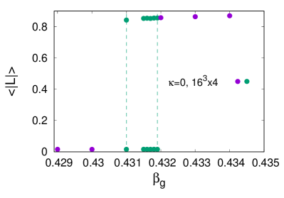
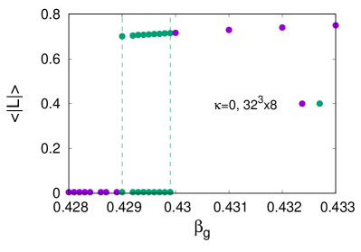
Figure 3: The average of the Polyakov loop vs $\beta_{g}$ for $N_{\tau}=$ 4 and 8.

The effect of the $\Phi$ field on the $CD$ transition and $Z_{2}$ symmetry is expected to depend on $\kappa$. To relate these two aspects of pure gauge theory to the phases of the Higgs field, simulations were performed to obtain the Higgs transition line. For a given $\beta_{g}$, $\kappa>\kappa_{c}$ corresponds to the Higgs broken phase. In this phase the action term dominates. For $\kappa<\kappa_{c}$ the fluctuations of the Higgs rather than the action dominate the thermodynamic properties. This situation is similar to the Ising model at high temperatures. In Fig.4 the Higgs transition line is plotted in the $\beta_{g}-\kappa$ plane. The location of the phase boundary is obtained by studying the $\kappa$ dependence of the interaction term and it’s fluctuations for different values of $\beta_{g}$. In our simulations the Higgs transition is found to be first order for intermediate range of $\beta$ and crossover for both small and large $\beta$, as observed in previous studies Jongeward:1980wx ; Creutz:1983ev . For large $\beta_{g}$ critical $\kappa_{c}$ remains flat and increases with $\beta_{g}$ in the small $\beta_{g}$ range. In our simulations the critical values ($\beta_{c},\kappa_{c}$) were found to vary mildly with $N_{\tau}$.

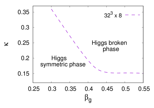
Figure 4: Phase diagram

In the Higgs broken phase, i.e large $\kappa$, the interaction term dominates over the entropy. The action takes the largest value when all the temporal links are $+1$. So it is expected that in the Higgs phase $Z_{2}$ symmetry is badly broken, also observed in our simulations. In the Higgs symmetric phase, it is the fluctuations of Higgs in other words the distribution of the interaction term dominate. In this phase there is a possibility for realisation of $Z_{2}$ symmetry. In figure. 5 we show $CD$ transition in the Higgs symmetric phase $(\kappa=.13)$. For comparison, $\kappa=0$ results also have been included. The $CD$ transition is first order even in the presence of $\Phi$, though the transition point shifts to lower values of $\beta_{g}$.

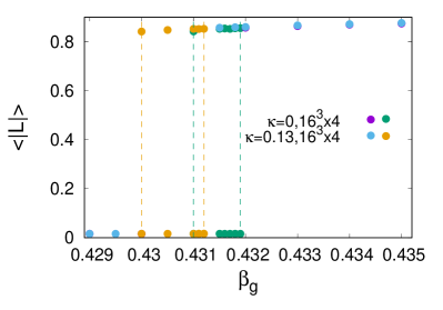
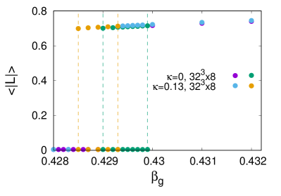
Figure 5: The average of the Polyakov loop vs $\beta_{g}$ for $N_{\tau}=$ 4 and 8.

To check the $N_{\tau}$ dependence of the $Z_{2}$ symmetry at $\kappa=.13$, the distribution of Polyakov loop is computed both in the confined and the deconfined phases for $N_{\tau}=2,3,$ and 8. In the deconfined phase, $L<0$ data is $Z_{2}$ rotated and then compared with $L>0$ data. The distributions/histograms are shown in figures. 7-11. For $N_{\tau}=2$ the histograms clearly show there is no $Z_{2}$ symmetry. In the deconfinement side there is no $Z_{2}$ symmetry as the two Polyakov loop sectors do not overlap. For $N_{\tau}=3$ the two peaks corresponding to the two sectors are approaching towards each other. For $N_{\tau}=8$, the histogram of Polyakov loop for two $Z_{2}$ sectors agree well with each other.

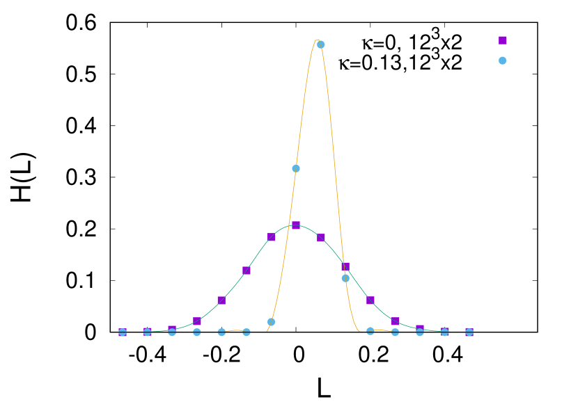
Figure 6: Histogram of L in the confined phase.

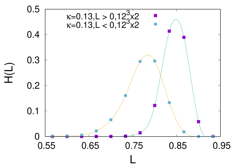
Figure 7: Histogram of L in the deconfined phase.

Figure 8: Histogram of L in the confined phase.

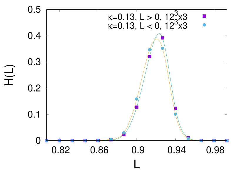
Figure 9: Histogram of L in the deconfined phase.

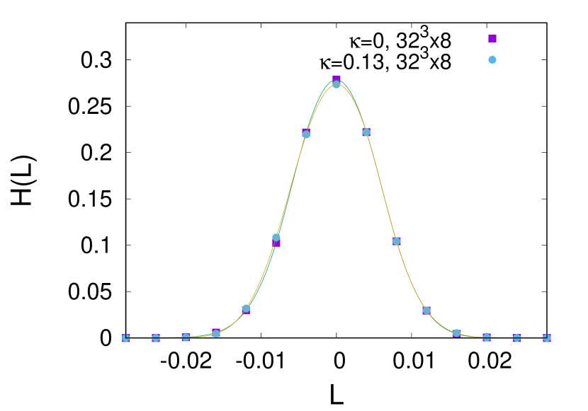
Figure 10: Histogram of L in the confined phase.

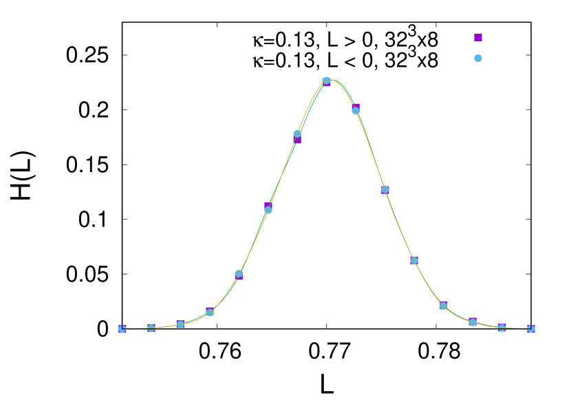
Figure 11: Histogram of L in the deconfined phase.

The $\kappa$ dependence of the $Z_{2}$ symmetry is studied by computing the thermal average of the temporal part of the interaction, i.e $sk_{4}=\sum_{n}\Phi_{n}U_{n,\hat{4}}\Phi_{n+\hat{4}}^{\dagger}$ and the corresponding susceptibility $\chi_{sk_{4}}$. These simulations are carried out in the deconfined phase, as there are two $Z_{2}$ states corresponding to each sector of the Polyakov loop. The results for ($\left<sk_{4}\right>,\chi_{sk_{4}}$) are shown in figures. 15-15. For all $N_{\tau}$ values the difference in ($\left<sk_{4}\right>,\chi_{sk_{4}}$) for these two sectors is vanishingly small for small enough $\kappa$. For larger $N_{\tau}$, the kappa value at which the two polyakov loop sectors differ significantly in $sk_{4}$ and $\chi_{sk_{4}}$ is higher. For the largest considered, $N_{\tau}=24$ , the two sectors agree in ($\left<sk_{4}\right>,\chi_{sk_{4}}$) up to the Higgs crossover point $\kappa<\kappa_{c}$. When Higgs transition is first order the $Z_{2}$ symmetry is observed in the Higgs symmetric phase even for $\kappa>\kappa_{c}$. Note that for $\kappa>\kappa_{c}$ the Higgs symmetric phase is meta-stable.

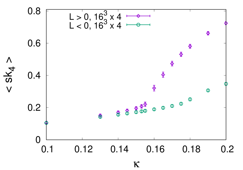
Figure 12: $sk_{4}$ average vs $\kappa$ for $\beta_{g}=0.435$ on $16^{3}\times 4$ lattice

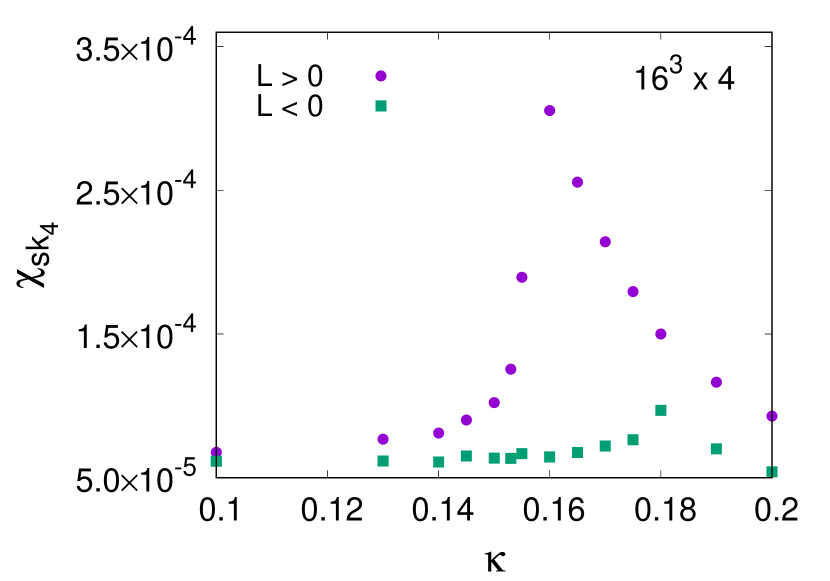
Figure 13: $sk_{4}$ fluctuation vs $\kappa$ for $\beta_{g}=0.435$ on $16^{3}\times 4$ lattice

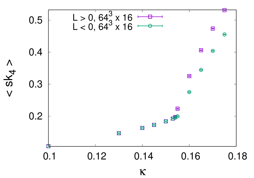
Figure 14: $sk_{4}$ average vs $\kappa$ for $\beta_{g}=0.435$ on $64^{3}\times 16$ lattice

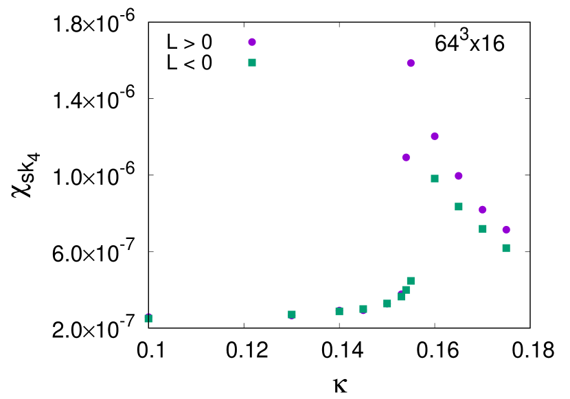
Figure 15: $sk_{4}$ fluctuation vs $\kappa$ for $\beta_{g}=0.435$ on $64^{3}\times 16$ lattice

It is clear from our $3+1$ dimensional simulations that the $Z_{2}$ symmetry is realised in the Higgs symmetric phase for large $N_{\tau}$, i.e the partition function averages of physical observables exhibit the $Z_{2}$ symmetry. Though we have focussed mostly on simulations around the Higgs transition region, it is important to look at the consequence of the $Z_{2}$ symmetry realisation across the CD transition. The CD transition line originates from the $\beta-$axis, runs parallel to $\kappa-$axis for small $\kappa$. For larger $\kappa$, $\beta_{g}=\beta_{c}$ decreases and the transition line merges with the Higgs transition line Jongeward:1980wx ; Creutz:1983ev . For small but non-zero $\kappa$ the CD transition is first order for $N_{\tau}\geq 3$. For large $N_{\tau}$, for $\beta_{g}\geq\beta_{c}$ the Polyakov loop distribution shows two $Z_{2}$ symmetric peaks. In the confined phase, for $\beta_{g}\leq\beta_{c}$, the distribution exhibits a single peak. With increase in $N_{\tau}$ the peak of the distribution steadily approaches $L=0$ and simultaneously the distribution exhibiting $Z_{2}$ symmetry.

For large $N_{\tau}$, below $\beta_{c}(N_{\tau})$ thermal average of the Polyakov loop $\langle L\rangle=0$. Note that $\langle L\rangle\propto Exp(-F/T)$, where $F$ is the free energy between static charges. This suggests that for $\beta\leq\beta_{c}(N_{\tau})$ static charges are confined. Previously confinement was observed only in the $\beta\to 0$ limit Fradkin:1978dv . It would be interesting to study the confinement aspects of the $Z_{N}$ symmetry realisation in $SU(N)$ gauge theories. For fixed $\kappa$ and $\beta$ in the confinement phase we observe that the free energy $F$ saturates for large $N_{\tau}$. This implies that the approach $\langle L\rangle\to 0$ is merely due to the temperature $T\to 0$.

To understand the realisation of $Z_{2}$ symmetry in the current theory, we consider a $0+1$ dimensional model keeping only the temporal component of the interaction term corresponding to a single spatial coordinate in the following section.

IV The partition function and density of states in $0+1$ dimensions

The temporal component of the gauge Higgs interaction corresponding to a particular spatial site can be written as,

$$S_{1D}=-\kappa sk_{4},~{}~{}~{}sk_{4}=\sum_{n=1}^{N_{\tau}}\Phi_{n}U_{n}\Phi_{n+1}.$$ (9)

$n$ denotes the temporal lattice site, i.e $1\leq n\leq N_{\tau}$. $\Phi_{n}$ satisfies the periodic boundary condition $\Phi_{N_{\tau}+1}=\Phi_{1}$. Since the action will not be invariant if a $z=-1$ gauge transformation is made on $U_{i}$’s, the action breaks the $Z_{2}$ symmetry explicitly. For this model the Polyakov loop can take values $\pm 1$. To see the $N_{\tau}$ dependence of the $Z_{2}$ symmetry we calculate the free energy $V(L,N_{\tau})$. To simplify the calculations we set $U_{i}=1$, for $i=1,2,...N_{\tau}-1$ and $U_{N_{\tau}}=L$. All other configurations of $U_{i}$ corresponding to a given value of $L$ are gauge equivalent. Now the partition function for $L=1$ is nothing but that of the one dimensional Ising chain. For $L=-1$ the only difference is that the coupling between $\Phi_{N_{\tau}}$ and $\Phi_{1}$ is anti-ferromagnetic. For each choice of $L$ the partition function can be calculated exactly, i.e,

$${\cal Z}(L=1)=\lambda_{1}^{N_{\tau}}+\lambda_{2}^{N_{\tau}},~{}~{}{\cal Z}(L=-1)=\lambda_{1}^{N_{\tau}}-\lambda_{2}^{N_{\tau}},$$ (10)

where $\lambda_{1}=e^{\kappa}+e^{-\kappa}$ and $\lambda_{2}=e^{\kappa}-e^{-\kappa}$. The corresponding free energies in the large $N_{\tau}$ limit are given by,

$$V(L=1)=V(L=-1)=-TN_{\tau}{\rm log}(\lambda_{1}).$$ (11)

This results show that there is $Z_{2}$ symmetry in $0+1$ dimensions in the limit of $N_{\tau}\to\infty$.

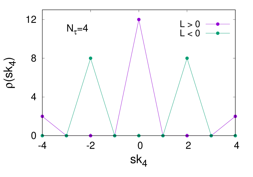
Figure 16: $\rho(sk_{4})$ for $\kappa=0$ in 0+1

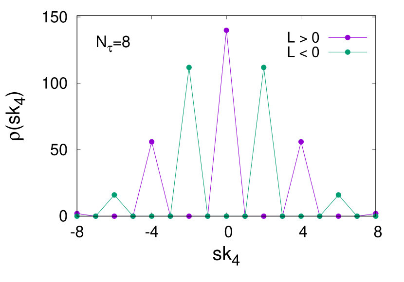
Figure 17: $\rho(sk_{4})$ for $\kappa=0$ in 0+1

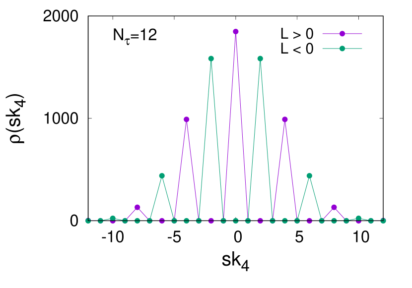
Figure 18: $\rho(sk_{4})$ for $\kappa=0$ in 0+1

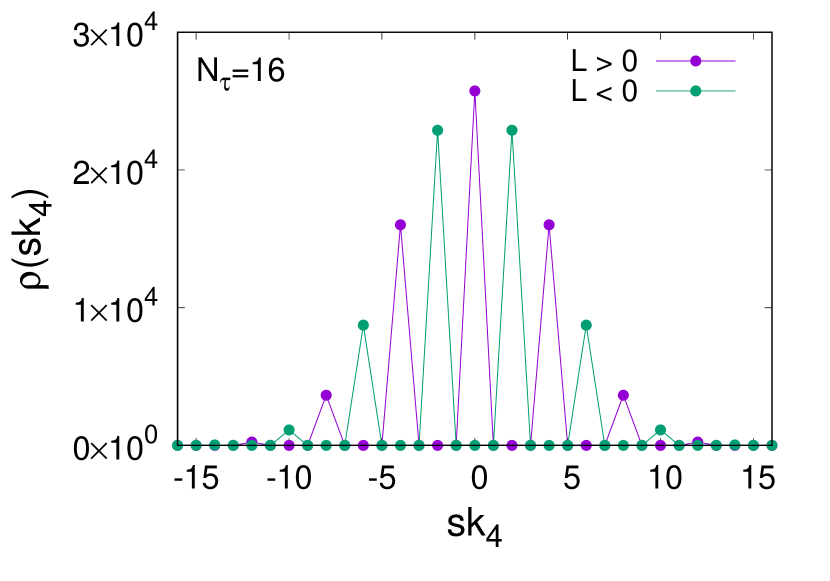
Figure 19: $\rho(sk_{4})$ for $\kappa=0$ in 0+1

As noted previously the realisation of the $Z_{2}$ symmetry (vanishingly small explicit breaking) must come from the $Z_{2}$ symmetry of the entropy or the $DoS$. For $L=1$ the sequence of allowed value of $sk_{4}$ is $\{N_{\tau},N_{\tau}-4,......\geq-N_{\tau}\}$. On the other hand for $L=-1$ the corresponding sequence is $\{N_{\tau}-2,N_{\tau}-6,........\geq 2-N_{\tau}\}$. The $DoS$ or $\rho(sk_{4})$ for $N_{\tau}=4,8,12$ and $16$ are shown in figures.19-19. For small $N_{\tau}$ there are clear difference for $L=\pm 1$. The difference persists for the largest as well as smallest values of $sk_{4}$. For large $N_{\tau}$, $\rho(sk_{4})$’s for both $L=\pm 1$ are well described by a gaussian centred at $sk_{4}=0$, with $\sqrt{N_{\tau}}$ as standard deviation. The logarithm of the peak hight is given by $~{}\simeq{\rm log}N_{\tau}!-2{\rm log}(N_{\tau}/2)!+{\rm log}2$ for $N_{\tau}$ even. For $N_{\tau}=2n+1$ the same can be approximated by ${\rm log}N_{\tau}!-{\rm log}(n^{2}+n)+{\rm log2}$. The thermodynamics in the $N_{\tau}\to\infty$ limit will be dominated by peak height and distribution of $\rho(sk_{4})$ around the peak, which is $Z_{2}$ symmetric, for all finite $\kappa$. Interestingly this situation is similar to one dimensional Ising chain where entropy dominates for any non-zero finite temperature.

In order to take into account the effect of nearest neighbour coupling along the spatial direction we consider $1+1$ dimensional model with $N_{s}=2$ and vary $N_{\tau}$. In this case the Polyakov loop can take value $L=0,\pm 2$. The exact calculation of $\rho(sk)$ get increasingly difficult with $N_{\tau}$. One can however consider generating configurations randomly by giving equal probability for each allowed value of a given variable. The results for the distribution of the total action for $N_{\tau}=4$ and $N_{\tau}=16$ are shown in Figs.21-21. As one can see that for higher $N_{\tau}$, $\rho(sk)$ around the peak $sk=0$ do not depend on $L$.

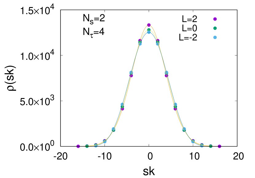
Figure 20: $\rho(sk)$ for $\kappa=0$ in 0+1

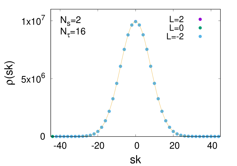
Figure 21: $\rho(sk)$ for $\kappa=0$ in 0+1

To find out how well the $\rho(sk_{4})$ describe the Monte Carlo simulations of the $4D$ partition function, the thermal average of the distribution function $H(sk_{4})$ of $sk_{4}$ has been computed. For each configuration $H(sk_{4})$ is given by the number of spatial sites with a given value of $sk_{4}$. Note that the distribution of $sk_{4}$ takes into account the Boltzmann factor which shifts the peak of $\rho(sk_{4})$ to the right.

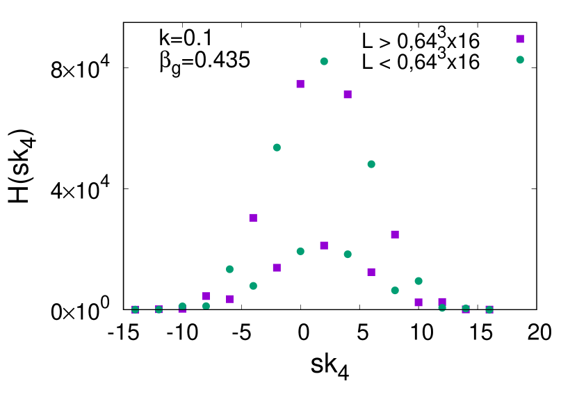
Figure 22: $H(sk_{4})$ for $\kappa=0.1,~{}\beta_{g}=0.435$ for $3+1$ dimension

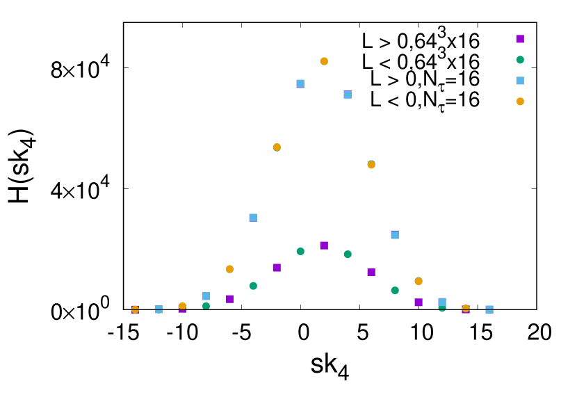
Figure 23: $H(sk_{4})$ fitted with $0+1$ density of states with a Boltzmann factor

The figure. 23 shows the distribution $H(sk_{4})$ for $N_{\tau}=16$ at $\kappa=0.1$ and $\beta_{g}=0.435$. For these values of $\kappa$ and $\beta_{g}$, the system is found to be in the deconfined and Higgs symmetric phase. The thermal average of the Polaykov loop for the two sectors are found to be $\left<L\right>=0.5896\pm 0.002$ and $-0.5897\pm 0.00199$. Since the $\left<L\right>\neq 1$ there is a smaller but finite fraction of spatial site where the Polyakov loop takes opposite value. This results in the lower envelope in $H(sk_{4})$. The results clearly show that $H(sk_{4})$ for both the Polyakov loop sectors can be approximately described by single function in other words the presence of $Z_{2}$ symmetry.

In figure. 23, we try to fit the $3+1$ dimensional simulation result with $0+1$ dimensional $DoS$ by including an extra Boltzmann factor, i.e exp$(\kappa^{\prime}sk_{4})$. The resulting fit agree very well with $H(sk_{4})$. We expect that the $0+1$ results can describe the $3+1$ Monte Carlo simulations in most of the phase diagram except for critical points. Note here, $H(sk_{4})$ values correspond to $\kappa=0.1$, however to fit $DoS$ one needs a $\kappa$ value which is higher. This is due to the fact that in $3+1$ dimensions $sk_{4}$ at a given spatial point interacts with $sk_{4}$ at the nearest neighbour sites. Considering a mean-field approximation one can compute the free energy difference between $L=1$ and $L=-1$ at $\kappa=\kappa^{\prime}$ for the $3+1$ dimensional system at $\kappa=0.1$, which turns out to be $10^{-10}$.

V Conclusions

In this paper the CD transition and $Z_{2}$ symmetry are studied in $Z_{2}$+Higgs theory in four dimensional space. The results show that for large $N_{\tau}$ the $Z_{2}$ symmetry is realised in the Higgs symmetric phase within statistical errors. To understand the mechanism of emergence of the $Z_{2}$ symmetry a simplified one dimension model of $Z_{2}+$Higgs is considered by keeping only the temporal interaction terms at a given spatial site. The partition function and the corresponding free energy for each of the two Polyakov loop sectors is exactly calculated. It is shown that the free energy difference between the two Polyakov loop sectors vanishes in the large $N_{\tau}$ limit, which leads to $Z_{2}$ symmetry purely due to dominance of entropy. The $DoS$ for finite $N_{\tau}$ are calculated exactly where the asymmetry between the different Polyakov loop sectors rapidly decreases with $N_{\tau}$. The effect of nearest neighbour interaction along the spatial directions in a simple model shows the persistence of $Z_{2}$ symmetry in the $DoS$. Further it is shown that the $3+1$ Monte Carlo simulations can be reproduced using the $DoS$ of the one dimensional model.

For a better understanding of the effects of $Z_{2}$ or $Z_{N}$ realisation on the confinement of static charges need to be studied in $SU(N)$ gauge theories in view of the $Z_{2}+$Higgs results, which we plan to do in future. The realisation of $Z_{N}$ symmetry due to dominance of $DoS$, it’s effect on the CD transition and the $Z_{N}$ states in the deconfined phase will play an important role in the study of the early Universe.

REFERENCES

REFERENCES

- (1) G. ’t Hooft, Nucl. Phys. B 138, 1-25 (1978) doi:10.1016/0550-3213(78)90153-0
- (2) L. D. McLerran and B. Svetitsky, Phys. Rev. D 24, 450 (1981) doi:10.1103/PhysRevD.24.450
- (3) V. M. Belyaev, Phys. Lett. B 254, 153-157 (1991) doi:10.1016/0370-2693(91)90412-J
- (4) J. B. Kogut, Rev. Mod. Phys. 51, 659 (1979) doi:10.1103/RevModPhys.51.659
- (5) J. Kuti, J. Polonyi and K. Szlachanyi, doi:10.1016/0370-2693(81)90987-4
- (6) L. D. McLerran and B. Svetitsky, doi:10.1016/0370-2693(81)90986-2
- (7) N. Weiss, Phys. Rev. D 24, 475 (1981) doi:10.1103/PhysRevD.24.475
- (8) M. Creutz, Phys. Rev. D 21, 2308-2315 (1980) doi:10.1103/PhysRevD.21.2308
- (9) B. Svetitsky and L. G. Yaffe, Nucl. Phys. B 210, 423-447 (1982) doi:10.1016/0550-3213(82)90172-9
- (10) L. G. Yaffe and B. Svetitsky, Phys. Rev. D 26, 963 (1982) doi:10.1103/PhysRevD.26.963
- (11) B. Svetitsky, Phys. Rept. 132, 1-53 (1986) doi:10.1016/0370-1573(86)90014-1
- (12) T. Celik, J. Engels and H. Satz, Phys. Lett. B 125, 411-414 (1983) doi:10.1016/0370-2693(83)91314-X
- (13) N. Weiss, Phys. Rev. D 25, 2667 (1982) doi:10.1103/PhysRevD.25.2667
- (14) V. M. Belyaev, I. I. Kogan, G. W. Semenoff and N. Weiss, Phys. Lett. B 277, 331-336 (1992) doi:10.1016/0370-2693(92)90754-R
- (15) Y. Guo and Q. Du, JHEP 05, 042 (2019) doi:10.1007/JHEP05(2019)042 [arXiv:1810.13090 [hep-ph]].
- (16) F. Green and F. Karsch, Nucl. Phys. B 238, 297-306 (1984) doi:10.1016/0550-3213(84)90452-8
- (17) F. Karsch, E. Laermann, A. Peikert, C. Schmidt and S. Stickan, Nucl. Phys. B Proc. Suppl. 94, 411-414 (2001) doi:10.1016/S0920-5632(01)00988-4 [arXiv:hep-lat/0010040 [hep-lat]].
- (18) H. Satz, Phys. Lett. B 157, 65-69 (1985) doi:10.1016/0370-2693(85)91213-4
- (19) M. Biswal, S. Digal and P. S. Saumia, Nucl. Phys. B 910, 30-39 (2016) doi:10.1016/j.nuclphysb.2016.06.025 [arXiv:1511.08295 [hep-lat]].
- (20) M. Biswal, M. Deka, S. Digal and P. S. Saumia, Phys. Rev. D 96, no.1, 014503 (2017) doi:10.1103/PhysRevD.96.014503 [arXiv:1610.08265 [hep-lat]].
- (21) R. Balian, J. M. Drouffe and C. Itzykson, Phys. Rev. D 10, 3376 (1974) doi:10.1103/PhysRevD.10.3376
- (22) R. Balian, J. M. Drouffe and C. Itzykson, Phys. Rev. D 11, 2104 (1975) [erratum: Phys. Rev. D 19, 2514 (1979)] doi:10.1103/PhysRevD.11.2104
- (23) M. Creutz, doi:10.1103/PhysRevD.21.1006
- (24) E. H. Fradkin and S. H. Shenker, Phys. Rev. D 19, 3682-3697 (1979) doi:10.1103/PhysRevD.19.3682
- (25) D. J. E. Callaway and L. J. Carson, Phys. Rev. D 25, 531-537 (1982) doi:10.1103/PhysRevD.25.531
- (26) G. Bhanot and B. A. Freedman, Nucl. Phys. B 190, 357-364 (1981) doi:10.1016/0550-3213(81)90566-6
- (27) G. Bhanot and M. Creutz, BNL-27833.
- (28) G. A. Jongeward and J. D. Stack, Phys. Rev. D 21, 3360 (1980) doi:10.1103/PhysRevD.21.3360
- (29) M. Creutz, L. Jacobs and C. Rebbi, Phys. Rept. 95, 201-282 (1983) doi:10.1016/0370-1573(83)90016-9
- (30) M. Caselle and M. Hasenbusch, Nucl. Phys. B 470, 435-453 (1996) doi:10.1016/0550-3213(96)00161-7 [arXiv:hep-lat/9511015 [hep-lat]].
- (31) M. Creutz, L. Jacobs and C. Rebbi, Phys. Rev. Lett. 42, 1390 (1979) doi:10.1103/PhysRevLett.42.1390
- (32) W. K. Hastings, Biometrika 57, 97-109 (1970) doi:10.1093/biomet/57.1.97
- (33) J. Engels, F. Karsch and H. Satz, Nucl. Phys. B 205, 239-252 (1982) doi:10.1016/0550-3213(82)90387-X
- (34) P. H. Damgaard and U. M. Heller, Phys. Lett. B 171, 442-448 (1986) doi:10.1016/0370-2693(86)91436-X