We present a general method to derive the appropriate Darmois-Israel junction conditions for gravitational theories with higher-order derivative terms by integrating the bulk equations of motion across the singular hypersurface. In higher derivative theories, the field equations can contain terms which are more singular than the Dirac delta distribution. To handle them appropriately, we formulate a regularization procedure based on representing the delta function as the limit of a sequence of classical functions. This procedure involves imposing suitable constraints on the extrinsic curvature such that the field equations are compatible with the singular source being a delta distribution. As explicit examples of our approach, we demonstrate in detail how to obtain the generalized junction conditions for quadratic gravity, $\mathcal{F}(R)$ theories, a 4D low-energy effective action in string theory and action terms that are Euler densities. Our results are novel, and refine the accuracy of previously claimed results in $\mathcal{F}(R)$ theories and quadratic gravity. In particular, when the coupling constants of quadratic gravity are those for the Gauss-Bonnet case, our junction conditions reduce to the known ones for the latter obtained independently by boundary variation of a surface term in the action. Finally, we briefly discuss a couple of applications to thin-shell wormholes and stellar models.

1 Introduction

In general relativity, the Darmois-Israel junction conditions prescribe the appropriate boundary conditions across a singular hypersurface $(\Sigma)$ supported by a localized energy-momentum source that contains a Dirac delta distribution. Apart from metric continuity at $\Sigma$, these ‘junction conditions’ can be expressed simply as the following equation

$$[K]h_{ij}-[K_{ij}]=8\pi S_{ij},\qquad K\equiv K^{m}_{m},$$ (1.1)

where the square bracket indicates the jump discontinuity across $\Sigma$, $h_{ij}$ is the induced metric, $S_{ij}$ is the singular Dirac delta source localized within $\Sigma$, and all indices pertain to coordinates of $\Sigma$. The Darmois-Israel junction conditions in (1.1) were historically obtained in [1, 2, 3] by integrating the field equations across the infinitesimal width of $\Sigma$, and were later shown to equivalently follow from the boundary variation of the Gibbons-Hawking-York term in the action [4, 5].

Since its discovery, (1.1) has found numerous applications in a plethora of gravitational topics, being primarily used to govern the construction of spacetime geometries obtained by a ‘cut-and-paste’ approach with $\Sigma$ as the locus of identification. These geometries include thin-shell wormholes [6] (and their other variants such as gravastars [7, 8]), static and dynamical stellar models [9, 10] like the Oppenheimer-Snyder solution [11] describing gravitational collapse, as well as domain wall configurations [12] separating true and false vacua in cosmology.

In recent years, there have been interesting explorations of generalizing (1.1) to the wider context of gravitational theories beyond Einstein’s theory which we can consider to be a long-distance, effective description connected to some presumably UV-complete framework of quantum gravity such as string theory. When interpreted as such, from the effective field theory perspective, it is natural to consider adding higher-derivative terms to the Einstein-Hilbert action. Models that have attracted interest include supergravity, $\mathcal{F}(R)$-theories, Gauss-Bonnet gravity, etc. Accordingly, there has been a small number of different proposals for how (1.1) should be modified in several contexts. For example, junction conditions were proposed in [13, 14, 15] for $\mathcal{F}(R)$ gravity, and in [16, 17] for quadratic gravity. However, we find these results to be incomplete as they miss contributions which can only be seen with a proper and careful treatment of terms involving products of the step function, Dirac delta function, and their derivatives. For example, consider the case that the extrinsic curvature is discontinuous across a hypersurface: $K_{ij}=K^{-}_{ij}+[K_{ij}]\Theta(n)$, where $n$ is the normal coordinate and $\Theta$ is the step function [13, 18] with $\Theta(0^{-})=0$, $\Theta(0^{+})=1$ and $K^{\pm}_{ij}\equiv K_{ij}(0^{\pm})$. The Gauss-Codazzi relation $R=\hat{R}-K^{2}-2\partial_{n}K-K_{ab}K^{ab}$ implies that

$$R=R^{+}\Theta+R^{-}(1-\Theta)-[K_{ab}][K^{ab}](\Theta^{2}-\Theta).$$ (1.2)

Naively, one may take

$$\Theta^{2}=\Theta.$$ (1.3)

However the field equations in higher derivative gravity theory imply that generally, these terms are not isolated. Instead, they appear together with delta functions and their derivatives (this will be discussed extensively below in Section 2). As a result, (1.3) cannot be taken prematurely from the outset as was assumed in [13, 18]. In fact, in any sensible regularization of the delta function, we have $\delta(n)=\Theta^{\prime}(n)$ and $\int dn\,\,\,\Theta^{n}(n)\delta(n)=\frac{1}{n+1}.$ This implies that in the distributional sense,

$$\delta(n)\left(\Theta^{2}(n)-\Theta(n)\right)\neq 0.$$

In Section 4.1.1 below, we show how the correct treatment of the $(\Theta^{2}-\Theta)$-term in (1.2) leads to contributons of the form $[K_{ij}][K_{ab}][K^{ab}]$ in the junction conditions of the $R^{2}$-theory. Such contributions were missed in the literature [13, 14, 16]. As products of singular distributions is unavoidable in higher derivative gravity and the handling of them are subtle, one of the key motivations of this work is to provide a consistent mathematical framework for the derivation of the junction conditions.

In this paper, we present a general method to derive the appropriate junction conditions for gravitational theories with higher-order derivative terms by integrating the bulk equations of motion across the infinitesimal width of the singular surface $\Sigma$, in the same spirit as was done in the foundational paper of Israel in [2]. Fundamentally, asserting an equivalence between both sides of the field equations in the sense of distribution translates to ensuring the convergence of the integral which is now much more complicated by virtue of the higher-order differential operators. Completing the integral then yields the generalized junction conditions compatible with a Dirac $\delta$-distribution carried by the energy-momentum tensor.

We find that a combination of the following techniques furnishes an effective toolbox for solving this problem. First, we choose to work in Gaussian normal coordinates describing a local neighborhood of $\Sigma$ which is now defined by taking $n=0$, where $n$ parametrizes the proper distance along a geodesic orthogonal to $\Sigma$. In this chart, we invoke the Gauss-Codazzi relations extensively to express various curvature terms in the equations of motion in terms of the intrinsic geometric quantities of $\Sigma$, the extrinsic curvature and their derivatives. The problem is now reduced to examining the convergence of a one-dimensional integral. For this purpose, we find that expressing the $\delta$-function as a limit of a sequence of classical functions gives us a powerful language for organizing various integrand terms according to their algebraic order of singularity. This allows us to identify what are the additional conditions on the embedding geometry that naturally ensure the absence of singular terms that are incompatible with a $\delta$-distribution source term. We call these conditions ‘regularity constraints’, and they are typically expressed as the vanishing of some function of the extrinsic curvature components on each side of $\Sigma$. As we shall elaborate later on, it turns out that they are intimately related to the Hadamard regularization procedure [19] in the theory of distributions (see e.g. [20]). In the absence of the regularity constraints, the generalized junction conditions are precisely the Hadamard-finite part of the integral. Our method can be readily adopted and applied to a wide variety of gravitational theories, including matter and gauge couplings, although in this paper, we focus almost exclusively on action terms that are invariants constructed from the Riemann tensor as illustrative examples.

Our exposition is structured as follows. In Section 2, we present the background canvas of concepts underlying our general approach of deriving the junction conditions via a bulk integration across $\Sigma$, including the notion of delta-convergent sequences, regularity constraints and how our method relates to Hadamard regularization. Section 3 contains a detailed derivation of the junction conditions for quadratic gravity. This is accompanied by Appendix A containing some integral identities that we developed for our purpose, and by Appendix B containing details of how the junction conditions in quadratic gravity reduce consistently to known ones for Gauss-Bonnet gravity. Section 4 presents the junction conditions for three types of theories: $\mathcal{F}(R)$ theories, a low-energy effective action descending from string theory, and higher-dimensional Euler density terms that appear in Lovelock gravity. In Section 5, we briefly discuss a couple of applications by examining how thin-shell wormholes and stellar models are governed by junction conditions in the context of $\mathcal{F}(R)=R+\beta R^{2}$ theory. Finally, we end with some concluding remarks in Section 6. For the reader who is uninterested in the illustrative examples of gravitational theories we have chosen, Section 2 suffices as a stand-alone explanation of the tapestry of techniques used in our method, but in our opinion, reviewing a couple of concrete examples in Section 3 or 4 should still be useful towards learning how to apply our method for other theories.

Conventions: We work in natural units where $\mathcal{G}=c=1$. Greek indices refer to all of spacetime, whereas Latin indices pertain to coordinates of the singular hypersurface $\Sigma$, with ‘$n$’ reserved for the direction normal to $\Sigma$. Our convention for the Riemann tensor is ${R^{\rho}}_{\sigma\mu\nu}=\partial_{\mu}\Gamma^{\rho}_{\nu\sigma}+\ldots$. Comparison with the existing results

Our results for $\mathcal{F}(R)$ theory and quadratic gravity refine the accuracy of those reported earlier in literature in a number of ways. For clarity, they are collected here:

1. As mentioned above, we explain in Section 4.1.1 explicitly the origin of a missing term in [13, 14, 16] for junctions conditions in the theory with $R^{2}$ action term.

2. In the papers [13, 15, 16, 17], the authors argued that the naive appearance of products of delta function and delta derivatives in the equations of motion leads to inconsistency, and that there is no unambiguous manner to sum them up. As a result it was assumed that $[K]=0$ so that $R$ is non-singular. On this issue, we find that the use of delta-convergent sequences clearly quantifies the growth property of each integrand term, and provides an organizational principle for identifying regularity constraints and a well-defined procedure to sum up the residual finite terms, eventually leading us to the junction conditions. For us, singularities are handled by a careful procedure of regularization. This is inspired by the common practice of regularization in quantum field theory. We will show below that, rather than insisting on the use of distribution-valued curvature, our approach is more practical and much less restrictive and allows for more general solutions to the theory.

3. In [16], the authors posited that in quadratic gravity, the energy-momentum tensor should contain the distributional derivative of the $\delta$-function that they derived from the higher-order differential operators acting on a discontinuous Riemann tensor. In this paper, we focus only on the explicit form of the generalized junction conditions, noting that only the delta-distribution component of $T_{\mu\nu}$ appears in final expression, since any regular component and those containing higher-order derivatives of the delta function do not survive the infinitesimal integral across $\Sigma$.

4. We should also mention that our method of derivation passes a stringent consistency test that is noticeably absent in the past literature, namely that when applied to quadratic gravity, i.e. taking the Lagrangian $\mathcal{L}=\beta_{1}R^{2}+\beta_{2}R^{\alpha\beta}R_{\alpha\beta}+\beta_{3}R^{\alpha\beta\mu\nu}R_{\alpha\beta\mu\nu}$, our junction conditions reduce to those of Gauss-Bonnet gravity $(\beta_{2}=-4\beta_{3}=-4\beta_{1})$ that were derived some time ago in [24] via a completely different approach — the boundary variation of a surface term [26] that accompanies the gravitational action. As already argued in [26, 27] and definitively shown in [28], the equations of motion of a generic higher-derivative gravitational theory do not descend from a well-posed variational principle with Dirichlet conditions, and hence the approach of obtaining their appropriate junction conditions by boundary variation of surface terms is not always applicable. An exception lies in the family of theories defined by Euler density terms which are the linear combinations of curvature invariants that generate only second-order field equations, and thus, in principle, these exists appropriate surface terms for them. The simplest example would be the Ricci scalar being the 2D Euler density, with the Gibbons-Hawking-York term $S_{GHY}=\frac{1}{8\pi}\int d^{d-1}x\,\,\sqrt{h}K$ being its surface term, and of which variation with respect to the induced metric yields (1.1). The junction condition derived in this manner nicely furnishes a consistency check for the other derivation route obtained by integrating across $\Sigma$. In Appendix B, we will demonstrate how the complicated junction conditions for a generic quadratic gravity theory reduce to the known ones for Gauss-Bonnet gravity. The regularity constraints need not be imposed precisely for $\beta_{2}=-4\beta_{3}=-4\beta_{1}$, and this also serves as a consistency check for the corresponding equations used in determining them. On this point, we note that previously in [16] where the authors proposed junction conditions for quadratic gravity, they imposed $[K_{ij}]=0$ even in the Gauss-Bonnet case which contradicts the known ones derived by a boundary variation [24, 25].

2 Generalized Junction Conditions - a general approach

2.1 Some Preliminaries

For a generic gravitational theory with higher-order derivatives of the metric in the action, let us denote the field equations as

$$\tilde{G}_{\mu\nu}\equiv R_{\mu\nu}-\frac{1}{2}Rg_{\mu\nu}+\ldots=8\pi T_{\mu\nu},$$ (2.1)

where the ellipses represent the additional terms descending from the modified action. In this work, we will mainly be studying gravitational theories where these terms are products of various contractions of the Riemann tensor and differential operators acting on them. On the RHS, we assume that the energy-momentum tensor harbors a singular source localized on some codimension one hypersurface $\Sigma$. If we integrate across the infinitesimal width of $\Sigma$, only singular terms on both sides of (2.1) survive and the resulting integral yields the appropriate junction conditions for the gravitational theory considered. The main purpose of this paper is to develop a conceptual and computational basis for this integration procedure. Fundamentally, apart from topological action terms which are not reflected in (2.1), the bulk equations of motion suffice as the starting point for the derivation of the junction conditions which can be regarded as consistency conditions for the bulk dynamics induced on $\Sigma$.

In the full generality, the induced metric on $\Sigma$ $h_{ij}$ can be timelike, spacelike or null. For the rest of the paper, we will mainly focus on the timelike case which has garnered the most interest in the past literature. When $\Sigma$ is endowed with a singular energy-momentum tensor localized on it, it represents a singular thin shell of matter. (For a spacelike $h_{ij}$, this would be a gravitational instanton whereas a null $h_{ij}$ would represent a singular light cone.)

In the most generic setting, $\Sigma$ is a codimension-one hypersurface that is embedded in a bulk manifold ($\mathcal{M}$) constructed from two distinct ones ($\mathcal{M}_{1},\mathcal{M}_{2}$) that is joined by identifying

$$\Sigma_{1}\sim\Sigma_{2}\sim\Sigma,$$

where $\Sigma_{1,2}$ are hypersurfaces in $\mathcal{M}_{1,2}$ that can be related via a homeomorphism. In this cut-and-paste procedure, the final manifold $\mathcal{M}$ is the union of $\Sigma$ and the interiors of $\mathcal{M}_{1,2}$ previously bounded by $\Sigma_{1,2}$. We can introduce a set of coordinates $(\zeta^{i})$ intrinsic to $\Sigma$ which is defined parametrically by

$$f\left(x^{\mu}(\zeta^{i})\right)=0,$$

with the induced metric

$$h_{ij}=g_{\mu\nu}\frac{\partial x^{\mu}}{\partial\zeta^{i}}\frac{\partial x^{\nu}}{\partial\zeta^{j}}.$$ (2.2)

Denoting the sign of $n^{2}$ by $\xi$, the unit normal vectors to $\Sigma$ read

$$n_{\mu}=\xi N\frac{\partial f}{\partial x^{\mu}},\qquad N=\left|g^{\alpha\beta}\partial_{\alpha}f\partial_{\beta}f\right|^{-1/2},\,\,\,\,n^{2}=\xi,$$

where $\xi=\{+1,-1,0\}$ for the cases of $\Sigma$ being timelike, spacelike and null respectively. The second fundamental form or the extrinsic curvature enacts an essential role in our discussion and can be defined as follows.

$$K_{ab}=h^{m}_{a}h^{l}_{b}\nabla_{m}n_{l},\qquad n^{a}K_{ab}=0.$$ (2.3)

For our purpose, we find it useful to work in the Gaussian normal coordinate system in the local neighborhood of $\Sigma$ constructed from the family of non-intersecting geodesics orthogonal to $\Sigma$.

$$ds^{2}=\xi dn^{2}+h_{ij}(n,x^{k})dx^{i}dx^{j},$$ (2.4)

with $\Sigma$ defined by taking $n=0$ and $x^{i}$ are the intrinsic coordinates. Having briefly described the geometric characterization of $\Sigma$, let us now return to the field equations in (2.1). On the RHS, we can express the energy-momentum tensor as

$$T_{\mu\nu}=S_{\mu\nu}\delta(n)+\ldots,$$

where we have denoted the delta function source by $S_{\mu\nu}=S_{\mu\nu}(\vec{x})$. The ellipses refer to regular components of the energy-momentum tensor, and more generally some linear combination of derivatives of the delta function. Working in the local Gaussian normal chart, we can integrate (2.1) across the infinitesimal width of $\Sigma$ as follows.

$$\lim_{\epsilon\rightarrow 0^{+}}\int^{\epsilon}_{-\epsilon}dn\,\,\tilde{G}_{\mu\nu}=8\pi S_{\mu\nu}.$$ (2.5)

The infinitesimal integral domain picks up only the $\delta$-distribution part of the energy-momentum tensor, since other components vanish in the $\epsilon\rightarrow 0$ limit. Formally, we can see this by writing

$$\lim_{\epsilon\rightarrow 0^{+}}\int^{\epsilon}_{-\epsilon}dn=\int^{\infty}_{-\infty}dn-\text{p.v.}\int^{\infty}_{-\infty}dn,$$

where the second term on the RHS is the Cauchy principal value of the first integral term. In local Gaussian normal coordinates, the Christoffel symbols read

$$\Gamma^{n}_{ij}=-\frac{1}{2}\partial_{n}h_{ij}=-K_{ij},\,\,\,\Gamma^{i}_{nj}=K^{i}_{j}=\frac{1}{2}h^{im}\partial_{n}h_{jm}.$$ (2.6)

The discontinuity in $\partial_{n}h_{ij}$ or the extrinsic curvature induces various singular terms in $\tilde{G}_{\mu\nu}$ which is then related to the singular source $S_{\mu\nu}$ in (2.5).

A main theme of this work is to seek the conditions characterizing the embedding of $\Sigma$, under which the LHS of (2.5) is well-defined. This then leads to an appropriate set of junction conditions on the LHS of (2.5) upon performing the integral. We take this to be the operational meaning of the delta function source in the energy-momentum tensor, since the field equations should be understood in the sense of distribution when the energy-momentum tensor carries a delta-singular source.

Now in our derivation, the Gauss-Codazzi relations turn out to be crucial as they express various curvature quantities in terms of the intrinsic Riemann tensor and the extrinsic curvature tensor, elucidating the form of various singular terms in $\tilde{G}_{\mu\nu}$ easily. Recall that the Gauss-Codazzi equations read

$$\hat{R}^{a}{}_{bcd} = \mathcal{P}\left({R^{a}}_{bcd}\right)+\xi\left(K^{a}_{c}K_{bd}-K^{a}_{d}K_{bc}\right),$$ (2.7)

$$n^{a}R_{aqrs}h^{q}_{b}h^{r}_{c}h^{s}_{d} = \xi\left(D_{d}K_{bc}-D_{c}K_{bd}\right),$$ (2.8)

where $\mathcal{P}$ refers to the indices being projected with the induced metric $h_{ab}$, $D_{a}$ is the projected covariant derivative defined with the induced metric and hatted variables are geometrical quantities intrinsic to $\Sigma$. Using Gaussian normal coordinates and contracting some of the indices, we further obtain the following useful set of equations.

$${R^{n}}_{snv} = \xi\left(-\partial_{n}K_{vs}+K_{av}K^{a}_{s}\right),\,\,\,R_{nijk}=D_{k}K_{ij}-D_{j}K_{ik},$$ (2.9)

$$R_{ij} = \xi\left(-\partial_{n}K_{ij}+2K^{a}_{j}K_{ai}-KK_{ij}\right)+\hat{R}_{ij},$$ (2.10)

$$R_{nn} = -\partial_{n}K-K^{ab}K_{ab}=-h^{ij}\partial_{n}K_{ij}+K^{ab}K_{ab},$$ (2.11)

$$R_{in} = D^{k}K_{ik}-D_{i}K,$$ (2.12)

$$R = \hat{R}-\xi\left(2\partial_{n}K+K^{2}+K^{ab}K_{ab}\right).$$ (2.13)

2.2 On the standard Darmois-Israel junction conditions in GR

It is instructive to first review how one can obtain the standard Darmois-Israel junction conditions in ordinary GR before proceeding to more complicated gravitational theories. In (2.5), we now simply take $\tilde{G}_{\mu\nu}=G_{\mu\nu}$ and integrate

$$\lim_{\epsilon\rightarrow 0^{+}}\int^{\epsilon}_{-\epsilon}dn\,\,G_{\mu\nu}=8\pi S_{\mu\nu}.$$ (2.14)

On the LHS, only singular terms in the Einstein tensor survive in the limit $\epsilon\rightarrow 0$. The singularity of these terms are of the Dirac delta type and can be traced to a discontinuity in the derivative of the metric in the direction normal to $\Sigma$ which, in the Gaussian normal chart, is effectively the discontinuous extrinsic curvature. We keep track of these terms appearing in the Einstein tensor which can be simplified to read

$$\xi\left(\partial_{n}K^{i}_{j}-\delta^{i}_{j}\partial_{n}K\right)+\xi\left(-KK^{i}_{j}+\ldots\right)=8\pi T^{i}_{j},$$ (2.15)

$$\xi\left(-\nabla_{i}K+\nabla_{j}K^{j}_{i}\right)=8\pi T^{n}_{i},\,\,\,-\frac{1}{2}\hat{R}+\frac{1}{2}\xi\left(K^{2}-\text{Tr}(K^{2})\right)=8\pi T^{n}_{n},$$ (2.16)

where the ellipses are terms which do not involve $\partial_{n}$. Integrating over $\Sigma$ as in (2.14) on both sides of the field equations then yields the junction conditions

$$\xi\left(-[K_{ij}]+[K]g_{ij}\right)=8\pi S_{ij},$$ (2.17)

which is the standard Darmois-Israel junction conditions in GR, and we have used the bracket $[...]$ to denote the jump or difference between the limiting values of the bracketed quantity on each side of $\Sigma$, for example $[K]\equiv K|_{n=0^{+}}-K|_{n=0^{-}}$. We also note that the junction conditions in other directions are trivial, i.e. in (2.5),

$$\lim_{\epsilon\rightarrow 0^{+}}\int^{\epsilon}_{-\epsilon}dn\,\,G_{in}=\lim_{\epsilon\rightarrow 0^{+}}\int^{\epsilon}_{-\epsilon}dn\,\,G_{nn}=0.$$ (2.18)

Thus in GR, the localized singular source $S_{\mu\nu}$ cannot have components non-parallel to $\Sigma$. As we shall see later, this is not generally true for other gravitational theories. Another feature characterizing the junction condition (2.17) that differentiates a generic higher-derivative theory from GR is that the junction equation does not only involve bracketed terms but also acquires terms that represent averaging across $\Sigma$.

A crucial ingredient in our formulation is a procedure that takes into account singular terms more divergent than delta function terms in the LHS of the field equations (2.1), that may appear in the equations of motion upon assuming a discontinuous extrinsic curvature (note that this problem is absent in (2.15)). We demonstrate how to impose suitable regularity constraints on the extrinsic curvature such that the integral in (2.5) remains convergent, leading to generalized junction conditions which are the appropriate boundary conditions at $\Sigma$. We will find that an essential tool is to regard the delta function as a limit of a sequence of absolutely convergent functions, a delicate subject which we turn to next.

2.3 Delta sequences and a double scaling limit

Since the singularities in (2.1) essentially arise from derivatives of the Heaviside step function parametrizing the discontinuity in the extrinsic curvature, we first consider a suitable representation of it by defining it as a limit $b\rightarrow 0$ of a sequence of classical functions $\Theta(n,b)$, with

$$\Theta(n)=\lim_{b\rightarrow 0}\Theta(n,b),\qquad\Theta(n,b)=\frac{1}{2}+\Theta_{X}\left(\frac{n}{b}\right),$$ (2.19)

where we have chosen to parametrize it such that its derivative yields a representation of the delta function as follows.

$$\delta(n)=\lim_{b\rightarrow 0}\partial_{n}\Theta(n,b)=\lim_{b\rightarrow 0}\frac{1}{b}\Theta^{\prime}_{X}\left(X\right)\equiv\lim_{b\rightarrow 0}\frac{1}{b}F(X),\qquad X\equiv\frac{n}{b},$$ (2.20)

The function $F(X)$ is sometimes known as a nascent delta function, with $\Theta_{X}(X)$ being its antiderivative. As a generalized function or distribution, we require that

$$\lim_{b\rightarrow 0}\int^{\infty}_{-\infty}dn\frac{1}{b}F(X)f(n)=f(0),$$ (2.21)

for all continuous $f(n)$ with compact support which implies that $F(X)$ is normalized as

$$\int^{\infty}_{-\infty}dX\,\,F(X)=1.$$ (2.22)

Formally, each nascent delta function gives rise to a distribution of the form

$$\tilde{f}_{1/b}=\partial_{n}\Theta(n,b)=\frac{1}{b}F(n/b),$$ (2.23)

and the sequence $\tilde{f}_{1},\tilde{f}_{2},\ldots$ converges to the delta function distribution $\delta(n)$ if the limit defined on the LHS on (2.21) exists. Some popular choices of the nascent delta function $F(X)$ appearing in related literature are (i) $\frac{1}{\sqrt{\pi}}e^{-X^{2}}$ (Gaussian distribution), (ii) $\frac{1}{\pi(1+X^{2})}$ (Cauchy distribution), (iii) $\frac{\sin(X)}{\pi X}$ (sinc function), etc. For the purpose of our work here, we adopt some choice of $F(X)$ that is even in $n$:

$$F(X)=F(-X),\,\,\,\Theta_{X}\left(X\right)=-\Theta_{X}\left(-X\right),$$ (2.24)

with $F(X)$ being infinitely differentiable, so that it is compatible with our use of its antiderivative $\Theta_{X}(X)$ to describe functions of varying degrees of smoothness.

Taking $F(X)$ to be an even function inherits the nature of $\delta(n)$ being an even distribution, and retains its original physical attribute of being symmetrical on either side of $\Sigma$. If we regard the nascent delta function as a probability density function describing how energy-mass is localized in $\Sigma$ (idealized by the $\delta$-distribution), then (2.24) translates to $n=0$ being the mean of the energy-mass distribution, which is expected on physical grounds. As we shall point out shortly in Section 2.4, the parity assignment (2.24) also leads to a natural generalization of the derivatives of the $\delta$-function when they are integrated against non-smooth functions.

Parametrizing the step function in this manner implies that for a function $g(n)$ which may not be smooth at (and after) a certain order of its derivative at $n=0$, we can consider it as the limit of a sequence of functions as follows.

$$g(n)=g_{1}(n)+\Theta(n)(g_{2}(n)-g_{1}(n))=\overline{g}(n)+\lim_{b\rightarrow 0}\Theta_{X}(X)[g(n)],$$ (2.25)

where $g_{1}(n),g_{2}(n)$ are infinitely differentiable functions of $n$ each analytically extending $g(n)$ beyond $n=0$ and we have defined

$$\overline{g}(n)=\frac{1}{2}\left(g_{1}(n)+g_{2}(n)\right),\quad[g(n)]=g_{2}(n)-g_{1}(n),\quad g_{2}(0)=g(0^{+}),\quad g_{1}(0)=g(0^{-}).$$

For example, if $g(n)$ is of class $C^{1}$ with its second-order derivative being discontinuous at $n=0$, then $g_{1}(0)=g_{2}(0),g^{\prime}_{1}(0)=g^{\prime}_{2}(0),g^{\prime\prime}_{1}(0)\neq g^{\prime\prime}_{2}(0)$, etc. One can perform ordinary derivatives on $g(n)$ before finally taking the $b\rightarrow 0$ limit.

In (2.5), the integrand is generally a rather complicated function of various non-smooth curvature quantities, and it is crucial that we apply (2.25) for all terms consistently before evaluating the integral. Formally, this procedure yields a sequence of regular distributions (which is essentially a complicated function of the nascent delta function and other functions of the metric tensor analytic at $\Sigma$) that ensure the convergence of (2.5).

We will find that this manner of expressing the step function (and hence the delta functions and their derivatives) lends us a powerful language for simplifying and organizing various types of singular terms consistently in the integrand of (2.5). It also necessitates a more precise prescription of the infinitesimal integration procedure in (2.5) , one which takes into account the relative scale separation between the sequence parameter $b$ and the infinitesimal width $\epsilon$ of the surface $\Sigma$. We now address this pivotal point that arises when we apply these considerations to our problem — the relative scaling of the thin-width parameter $\epsilon$ and the nascent delta function parameter $b$.

Recall that in deriving the junction equations, we perform an integral with limits parametrizing the width of the infinitesimally thin $\Sigma$, and hence we send the integral limits to zero after integrating. The integral preserves only terms which accompany a delta function singularity. Consider again (2.21) with an infinitely differentiable $f(n)$, but with the integral limits of (2.5). We still expect to recover $f(0)$ on the RHS. Expanding $f(n)$ around $n=0$ to obtain

$$\lim_{\epsilon\rightarrow 0}\lim_{b\rightarrow 0}\int^{\epsilon}_{-\epsilon}dn\,\,\delta_{b}(n)f(n)=\lim_{\epsilon\rightarrow 0}\lim_{b\rightarrow 0}\int^{\epsilon/b}_{-\epsilon/b}dy\,F(y)\left(f(0)+byf^{\prime}(0)+\frac{1}{2}b^{2}y^{2}f^{\prime\prime}(0)+\ldots\right),$$ (2.26)

we find that we recover (2.21) upon taking the double scaling limit

$$\epsilon\rightarrow 0,\qquad b/\epsilon\rightarrow 0.$$ (2.27)

We note that on the contrary, if we specify $b$ to vanish such that $b/\epsilon\rightarrow\mathcal{O}(1)$ or the converse $\epsilon/b\rightarrow 0$, then we do not recover $f(0)$. The physical reasoning behind (2.27) is simple and intuitive: the thin-width limit must be kept away from/taken after the limit of the sequence of nascent delta functions, or otherwise we are not genuinely integrating a singular delta function across $\Sigma$.

Recall that in the field equations, we seek a solution to

$$\tilde{G}_{\mu\nu}=R_{\mu\nu}-\frac{1}{2}Rg_{\mu\nu}+\ldots=8\pi\left(S_{\mu\nu}\delta(n)+\ldots\right),$$ (2.28)

where the ellipses refer to all regular components of the energy-momentum tensor and possibly a linear combination of higher-order derivatives of the delta function, all of which do not survive the integral of (2.5). A solution to (2.28) must thus integrate to give $S_{\mu\nu}$ in the following manner.

$$\lim_{\epsilon\rightarrow 0}\lim_{b\rightarrow 0}\int^{\epsilon}_{-\epsilon}dn\left(R_{\mu\nu}-\frac{1}{2}Rg_{\mu\nu}+\ldots\right)=8\pi S_{\mu\nu},$$ (2.29)

where the limit in $b$ is taken for the sequence of distributions defined by (2.23). We have to ensure that this sequence of integrals converges which generically requires additional conditions to be imposed on the extrinsic curvature for the integral in (2.29) to be well-defined.

This double scaling limit also preserves the fact that we can obtain a well-defined operational meaning for the derivatives of the delta functions when they are integrated against smooth functions, i.e. that we have, in a weak distributional sense,

$$\delta^{(k)}[g(n)]\sim(-1)^{k}g^{(k)}(0),$$ (2.30)

for a $g(n)$ analytic at $n=0$. This formula needs to be refined generally for a non-smooth $g(n)$ — an important yet tricky point that is relevant for us since, as we shall see, the equations of motion of higher-derivative gravitational theories typically contain terms which are products of non-smooth functions and a number of delta functions each equipped with some order of derivative.

2.4 Generalized distributions and regularity constraints

In this section, we present a well-defined procedure that extends the usual notion of distribution for the delta function (and its derivatives) to one that could be applied when they are integrated against non-smooth functions. Essentially for our purpose here, this will ultimately turn out to furnish a simple and clear method to identify and classify singular terms arising from the junction equations, leading to regularity constraints which we can impose on the extrinsic curvature to eliminate singular terms that render (2.5) to be ill-defined.

We begin with the basic examples of the $\delta(n),\delta^{\prime}(n)$.

2.4.1 Warm-up: more about $\delta(n),\delta^{\prime}(n)$

Let us consider a discontinuous test function for the delta function which we express as $f(n)=\overline{f}(n)+\Theta_{X}(X)[f(n)]$ where $\overline{f}(n)=\frac{1}{2}\left(f_{1}(n)+f_{2}(n)\right),[f(n)]=f_{2}(n)-f_{1}(n)$, with both $f_{1,2}(n)$ being smooth functions that extend $f(n)$ across $\Sigma$. Within the infinitesimal domain width, we can expand $f(n)$ about the origin. In the notations introduced in the previous section, we have

$$\lim_{\epsilon\rightarrow 0}\lim_{b\rightarrow 0}\int^{\epsilon}_{-\epsilon}dn\,\,f(n)\delta_{b}(n)=\lim_{\epsilon\rightarrow 0}\lim_{b\rightarrow 0}\sum_{l=0}\frac{b^{l}}{l!}\int^{\epsilon/b}_{-\epsilon/b}dX\,\,X^{l}F(X)\left(\overline{f}^{(l)}(0)+\Theta_{X}(X)[f^{(l)}(0)]\right)$$ (2.31)

The only non-vanishing term is $l=0$, and since $F(X),\Theta_{X}(X)$ are even and odd in $X$ respectively, we obtain

$$\lim_{\epsilon\rightarrow 0}\lim_{b\rightarrow 0}\int^{\epsilon}_{-\epsilon}dn\,\,f(n)\delta_{b}(n)=\overline{f}(0),$$ (2.32)

a result which is naturally intuitive and reduces correctly to the expected one in the continuous limit. Now we can extend this calculation to derivatives of the delta function, for example, $\delta^{\prime}(n)$. Consider thus the integral

$$\lim_{\epsilon\rightarrow 0}\lim_{b\rightarrow 0}\int^{\epsilon}_{-\epsilon}dn\,\,f(n)\delta^{\prime}_{b}(n)=\lim_{\epsilon\rightarrow 0}\lim_{b\rightarrow 0}\sum_{l=0}\frac{b^{l-1}}{l!}\int^{\epsilon/b}_{-\epsilon/b}dX\,\,X^{l}F^{\prime}(X)\left(\overline{f}^{(l)}(0)+\Theta_{X}(X)[f^{(l)}(0)]\right).$$ (2.33)

For all $l>1$ this vanishes. For $l=1$, since $F^{\prime}(X),\Theta_{X}(X)$ are both odd in $X$, this term reads

$$\int^{\infty}_{-\infty}dX\,XF^{\prime}(X)\overline{f}^{\prime}(0)=-\overline{f}^{\prime}(0),$$ (2.34)

where we have integrated by parts. We are left with the $l=0$ term which is singular since

$$\lim_{b\rightarrow 0}\frac{1}{b}\int^{\infty}_{-\infty}dX\,\,F^{\prime}(X)\left(\overline{f}(0)+\Theta_{X}(X)[f(0)]\right)=\lim_{b\rightarrow 0}\frac{[f(0)]}{b}\int^{\infty}_{-\infty}dX\,\,F^{\prime}(X)\Theta_{X}(X).$$ (2.35)

The integral is then well-defined only if we impose from the outset the continuity of $f$ at $n=0$,

$$f_{2}(0)=f_{1}(0),$$ (2.36)

leading to

$$\lim_{\epsilon\rightarrow 0}\int^{\epsilon}_{-\epsilon}dn\,\,f(n)\delta^{\prime}(n)=-\overline{f}^{\prime}(0).$$ (2.37)

The continuity condition in (2.36) for $\delta^{\prime}(n)$ is the simplest example of what we shall allude to as regularity constraints that we would need to solve for, and impose when we encounter some integrand in (2.5) that is typically a product of some nascent delta functions each possibly equipped with some order of derivative. Subject to (2.36), we can understand $\delta^{\prime}(n)$ to yield (minus) the average of the first derivative of $f(n)$ evaluated at $n=0$ should the function be non-differentiable at $n=0$. In a similar vein, one can prove that more generally, we have

$$\lim_{\epsilon\rightarrow 0}\int^{\epsilon}_{-\epsilon}dn\,\,f(n)\delta^{(k)}(n)=(-1)^{k}\overline{f}^{(k)}(0),\,\,\,k\geq 1,$$ (2.38)

which is an intuitive generalization of the case where the test functions $f(n)$ are smooth. We note that the simple form of the RHS of (2.38) follows by virtue of the symmetry property of the nascent delta function in (2.24) which, if relaxed, leads to a more complicated relation. For example, if $F$ has no definite parity, then generally instead of (2.37) we have $-\overline{f}^{\prime}(0)-[f^{\prime}(0)]\int^{\infty}_{-\infty}dXF^{2}(X)X$, which depends on the precise form of $F$.

Usually, when $\delta(n),\delta^{\prime}(n)$ are regarded as distributions on some open subset of $\mathbb{R}$, the class of test functions are smooth, compactly supported functions. As shown above, for test functions which are non-smooth, $\delta(n),\delta^{\prime}(n)$ can still be regarded as distributions with point support at $n=0$, but for $\delta^{\prime}(n)$ to be a sensible distribution, we need to restrict the class of test functions to be at least continuous at $n=0$.

2.4.2 Regularity constraints for products of nascent delta functions & their derivatives

In the Gaussian normal chart, integrating the bulk equations of motion (of a general higher-derivative gravitational theory) across $\Sigma$ is reduced to evaluating a set of one-dimensional integrals, with the integrand being some complicated product of various derivatives of the extrinsic curvature. Since generally, we take the extrinsic curvature to be not necessarily continuous at $\Sigma$ in response to a delta-singular energy source, this implies that in the absence of some regularizing constraints, such an integral is generically singular.

In the same vein by which we have studied the basic examples of $\delta(n),\delta^{\prime}(n)$, we now explain how we can solve for regularity constraints for products of non-smooth functions, delta functions and their derivatives. As we have seen in the previous examples, it is useful to describe a non-smooth function with the ansatz (2.25) which, in turn, contains smooth functions that can be expanded around $n=0$ within the thin-width domain of integral.

This implies that we can break down the integral in (2.5) into a linear combination of integrals of the following form.

$$I(l,\vec{k})=\lim_{\epsilon\rightarrow 0}\int^{\epsilon}_{-\epsilon}dn\,\,n^{l}\partial^{k_{1}}_{n}\Theta(n)\partial^{k_{2}}_{n}\Theta(n)\ldots\partial^{k_{j}}_{n}\Theta(n),$$ (2.39)

where $l$ and the indices $\vec{k}=\{k_{1},k_{2},\ldots,k_{j}\}$ are non-negative integers, with each $k_{i}$ indicating the order of derivative. Together with the scaling limit (2.27), we can express (2.39) as

$$I(l,\vec{k})=\lim_{b\rightarrow 0}b^{l+1-\sum^{j}_{m=1}k_{m}}\int^{\infty}_{-\infty}dX\,\,X^{l}\Theta_{X}^{(k_{1})}(X)\ldots\Theta_{X}^{(k_{j})}(X).$$ (2.40)

Such a term vanishes for $l\geq\sum_{m}k_{m}$, remains finite for $l+1-\sum_{m}k_{m}=0$, and diverges for

$$l+1-\sum^{j}_{m=1}k_{m}<0,\qquad l=j-\sum^{j}_{m=1}k_{m}\,\,\,\,\,(\text{mod}\,\,2),$$ (2.41)

with the second condition in (2.41) being due to the fact that the integral $I(l,\vec{k})$ vanishes by virtue of $\Theta_{X}(X)=-\Theta_{X}(-X)$ for $l=1+j-\sum_{m}k_{m}$    (mod 2).

After summing up the linear combination of $I(l,\vec{k})$ defining (2.5), for various singular terms which diverge as $b^{s}$ for some negative index $s$, we can now sum them up and set the overall coefficient to vanish. This naturally leads to a regularity constraint that we have to impose separately for each order of singularity labelled by each distinct $s$. A caveat is that the definite integral in (2.40) is generally representation-dependent. Since we would like to eliminate all singular integrals for any choice of nascent delta function, we should then impose a stronger condition: that for each family of integrals labelled by the same $\vec{k}$, every singular $l$ satisfying (2.41) then leads to a regularity constraint. This procedure then renders the integral in (2.5) to be well-defined for any choice of nascent delta function. In the following, we elaborate on several illustrative examples.

We begin with a basic example by taking $\vec{k}_{0}=\{1,1,1\}$, with

$$I(l,\vec{k}_{0})=\lim_{\epsilon\rightarrow 0}\int^{\epsilon}_{-\epsilon}dn\,\,n^{l}\,\left(\Theta^{\prime}(n)\right)^{3}=\lim_{b\rightarrow 0}b^{l-2}\int^{\infty}_{-\infty}dX\,\,X^{l}\,F^{3}(X),$$ (2.42)

which diverges for $l=0$, vanishes for $l=1$ and $l\geq 3$, and for $l=2$, it evaluates to $\int^{\infty}_{-\infty}dX\,\,X^{2}\,F^{3}(X)$. If we replace $n^{l}$ in the integrand of (2.42) by a function $\phi(n)$ that is analytic at $n=0$, then this implies that the integral diverges unless $\phi(0)=0$, in which case we have

$$I(\phi,\vec{k}_{0})\equiv\lim_{\epsilon\rightarrow 0}\int^{\epsilon}_{-\epsilon}dn\,\,\phi(n)\,\left(\Theta^{\prime}(n)\right)^{3}=\frac{\phi^{\prime\prime}(0)}{2}\int^{\infty}_{-\infty}dX\,\,X^{2}\,F^{3}(X).$$ (2.43)

In this case, $\phi(0)=0$ would be what we call as a regularity constraint which stipulates how fast $\phi(n)$ should grow near the origin for the integral to converge. The integral (2.43) also demonstrates that the naive product of three $\delta$-functions can be understood as a proper distribution, provided we restrict the space of test functions to be those which grow at least as $\phi(n)\sim n+\mathcal{O}(n^{2})$ near the origin. This serves as a simple example of how the use of nascent delta functions resolves the ‘ambiguity’ that may arise in interpreting products of $\delta$-functions as articulated in [16].

As an another example, consider the sum

$$\sum_{l}C_{l}I(l,\vec{k}),$$

with a fixed $\vec{k}$, the set of regularity constraints are simply

$$C_{l}=0,\qquad\forall\,l\,\,\,\text{satisfying}\,\,\,\eqref{diverge}.$$ (2.44)

In (2.5), as we shall see through explicit examples in later sections, it involves a linear combination of integrals of the form $I(l,\vec{k})$ with a finite set of $\vec{k}$. The entire set of regularity constraints is then the union of all (2.44) associated with each $\vec{k}$.

It is also instructive to check how (2.41) applies to the previous basic examples of $\delta(n),\delta^{\prime}(n)$ in (2.31) and (2.33). We note that for the two terms on the RHS of (2.31), they correspond to $I(l,\{1\})$ and $I(l,\{0,1\})$ in the notation of (2.39). With $\sum_{m}k_{m}=1$ for each term, there is no solution to (2.41) and thus no regularity constraint is needed. For (2.33), each of the two terms on the RHS are of the form $I(l,\{2\})$ and $I(l,\{0,2\})$ respectively, with $\sum_{m}k_{m}=2$ for each term. From (2.41), we thus see that there is a regularity constraint needed for $I(l,\{0,2\})$ (where $j=2$) associated with $l=0$, and this is simply (2.36).

After imposing the necessary regularity constraints in (2.5) following the above approach, we are left with a linear combination of well-defined integrals of the form

$$I(l,\vec{k})=I\left(\sum^{j}_{m=1}k_{m}-1,\vec{k}\right)=\int^{\infty}_{-\infty}dX\,\,X^{(\sum^{j}_{m=1}k_{m}-1)}\Theta_{X}^{(k_{1})}(X)\ldots\Theta_{X}^{(k_{j})}(X).$$ (2.45)

Since the integrand of (2.45) is odd for an even $j$, such a term only contributes to the junction equations for odd values of $j$. For example, in (2.31), the eventual expression corresponds to the first term within the RHS bracket which is of the form (2.45) with $l=0,j=1,\sum_{m}k_{m}=1$, whereas for (2.33), we note that (2.34) is of the form (2.45) with $l=1,j=1,\sum_{m}k_{m}=2$. As another example, for the sum $\sum_{l}C_{l}I(l,\vec{k})$, the only finite term (after imposing (2.44)) is

$$C_{r}I\left(r,\vec{k}\right),\qquad r=\sum^{j}_{m=1}k_{m}-1,$$ (2.46)

which is non-vanishing only if $j$ is odd. A caveat is that, like the definite integral in (2.41), an expression like (2.45) is generally sensitive to the choice of the nascent delta function, apart from terms like

$$\int dX\,\,\Theta^{\prime}_{X},\qquad\int dX\,\,X^{p}\Theta^{(p+1)}_{X},\qquad\text{or}\qquad\int dX\,\,\left(\Theta_{X}\right)^{p}\Theta^{\prime}_{X},$$ (2.47)

which are independent of the choice. For example, consider the integral

$$I(2,\{1,1,1\})=\int^{\infty}_{-\infty}dX\,\,X^{2}\left(\Theta^{\prime}_{X}(X)\right)^{3}.$$ (2.48)

If we pick the nascent delta function to be the Gaussian $F(X)=\frac{1}{\sqrt{\pi}}e^{-X^{2}}$, then (2.48) evaluates to $1/(6\pi\sqrt{3})$, whereas a choice of $F(X)=\frac{\sin(X)}{\pi X}$ yields $1/(2\pi^{2})$ instead. It may seem like such junction terms are ‘regularization-dependent’. This feature is obviously absent in ordinary GR, and here we see that the higher-order nature of the field equations may probe the form of the nascent delta function. To write down consistent junction conditions that are insensitive to the choice of nascent delta functions, we could additionally set the coefficient $C_{r}$ in (2.46) to vanish each time it appears in (2.5). We are then left with junction terms arising from universal terms like those in (2.47).

In most of our working examples for the rest of the paper, these representation-dependent terms turn out not to feature much. The only setting where it arises non-trivially in this work is the case of $R^{3}$ theory for which we find the terms

$$\int dX\,\Theta^{\prime 2}_{X}\Theta_{X}X,\qquad\int dX\,\Theta^{\prime\prime}_{X}\Theta^{\prime}_{X}\Theta_{X}X^{2},$$

to be manifest in the junction equations. As we shall demonstrate later, these terms would be absent if we further set $[K^{\prime}]=0$ as a regularity constraint for the $R^{3}$ theory’s junction equations. In the general case, our derivation procedure described above allows us to solve for the regularity constraints that will yield the final junction conditions to be representation-independent if desired. Nonetheless, it is noteworthy that the convergence of the integral (2.5) is compatible with the presence of these terms which, if allowed, implies that the specification of junction conditions is only complete with a choice of nascent delta function.

To summarize, we can now state explicitly how to read off the regularity constraints and junction conditions for (2.5). After parametrizing each discontinuous geometric quantity and its derivatives by $\Theta_{X}$, expanding the LHS of (2.5) would yield integrand terms typically of the form

$$I_{\vec{k}}\equiv\phi(n)\Theta^{(k_{1})}_{X}\Theta^{(k_{2})}_{X}\ldots\Theta^{(k_{j})}_{X},$$ (2.49)

for some vector index $\vec{k}$, with $\phi(n)$ analytic at $\Sigma$, then the regularity constraints associated with $I_{\vec{k}}$ are

$$\phi^{l}(0)=0,\,\,\,\forall\,\,l\leq\sum_{m=1}^{j}k_{m}-2,\,\,\,l=j-\sum_{m=1}^{j}k_{m}\,\,\,(\text{mod}\,\,2),$$ (2.50)

with the junction term induced by integrating $I_{\vec{k}}$ across $\Sigma$ being

$$J_{\vec{k}}=\frac{1}{((\sum_{m}k_{m})-1)!}\phi^{((\sum_{m}k_{m})-1)}(0)\left(\int^{\infty}_{-\infty}dX\,X^{(\sum_{m}k_{m})-1}\Theta^{(k_{1})}_{X}\ldots\Theta^{(k_{j})}_{X}\right).$$ (2.51)

The final junction condition arising from (2.5) is then the sum of all the junction terms, each of the form (2.51), subject to us imposing all the regularity constraints, each of the form (2.50).

2.5 The relation to Hadamard Regularization

In this Section, we point out a relation between the regularity constraints and Hadamard regularization [19] — a well-studied procedure to regularize divergent integrals typically encountered in the theory of singular integral operators, and also commonly invoked when one handles distributions defined by divergent integrals (for an emphasis in the theory of distributions, see for example [20]).

Let us first briefly review the notion of Hadamard regularization with a simple example. Consider the (divergent) integral

$$I_{H}=\int^{\infty}_{0}dx\,\frac{\phi(x)}{x^{3/2}}=\lim_{\epsilon\rightarrow 0}\int^{\infty}_{\epsilon}dx\,\frac{\phi(x)}{x^{3/2}},$$

where $\phi(x)$ is regular and continuous at the origin. From the mean value theorem, we can write $\phi(x)=\phi(0)+x\phi^{\prime}(tx)\equiv\phi(0)+x\varphi(x),\,\,\,0<t<1$ and thus we can express the above integral as

$$I_{H}=\lim_{\epsilon\rightarrow 0}\frac{2\phi(0)}{\epsilon}+\lim_{\epsilon\rightarrow 0}\int^{\infty}_{\epsilon}dx\,\,\frac{\varphi(x)}{\sqrt{x}}.$$ (2.52)

The second integral in (2.52) converges and we define it to be Hadamard finite part of $I_{H}$, writing

$$FP\int^{\infty}_{0}dx\,\,\frac{\phi(x)}{x^{3/2}}=\lim_{\epsilon\rightarrow 0}\int^{\infty}_{\epsilon}dx\frac{\phi(x)}{x^{3/2}}-\lim_{\epsilon\rightarrow 0}\frac{2\phi(0)}{\sqrt{\epsilon}}.$$ (2.53)

We have thus extracted the singular piece in the integral, with the first term of RHS of (2.53) being the residual finite integral. The above example can be generalized to a similar regularization of the divergent integral

$$I_{D}=\int^{\delta}_{-\delta}dx\,\,\,f(x)\phi(x),\qquad\delta>0,$$

where we take $\phi(x)$ to be analytic at the origin, and $f(x)|x|^{m}$ has an algebraic singularity of order $m$ at $x=0$, i.e. $m$ is some smallest positive integer such that $f(x)|x|^{m}$ is locally integrable.

We can extend this notion to $f(x)$ being a distribution, the Hadamard regularization of which is then defined as

$$FP\langle f,\phi\rangle=\int^{\delta}_{-\delta}dx\,\,f(x)\left(\phi(x)-\left(\phi(0)+\phi^{\prime}(0)x+\ldots+\frac{1}{m!}\phi^{(m-1)}(0)x^{m-1}\right)\right)\Theta\left(1-\frac{|x|}{\epsilon}\right).$$ (2.54)

We now examine how (2.54) is relevant for our context. From (2.39) and (2.40), we see that the sequence (in parameter $b$)

$$\Delta_{\vec{k}}(n,b)\equiv\Theta^{(k_{1})}(n,b)\ldots\Theta^{(k_{j})}(n,b),$$

converges to a distribution $\Delta_{\vec{k}}(n)$ that is of order of singularity $\left(\sum_{m=1}^{j}k_{m}\right)-1$, and further, upon integrating it against some function $\phi(n)$ that is analytic at $n=0$, the Hadamard-regularized distribution reads

$$FP\langle\Delta_{\vec{k}}(n),\phi(n)\rangle = \lim_{\epsilon\rightarrow 0}\int^{\epsilon}_{-\epsilon}dn\,\,\Delta_{\vec{k}}(n)$$

$$\times\Bigg{(}\phi(n)-\left(\phi(0)+\phi^{\prime}(0)n+\ldots+\frac{1}{(\sum_{m}k_{m}-2)!}\phi^{(\sum_{m}k_{m}-2)}(0)n^{\sum_{m}k_{m}-2}\right)\Bigg{)},$$

where now $\delta=\epsilon=0^{+}$ for the relevant integral domain. Comparing (2.5) against (2.50) and (2.51), and recalling that $I(l,\vec{k})$ vanishes for $l=1+j-\sum_{m}k_{m}\,\,(\text{mod}\,\,2)$, it is then clear that:

• in the absence of the regularity constraints, the junction condition is nothing but the Hadamard-finite part of the LHS of (2.5),

• imposing the regularity constraints then ensures that the integral in (2.5) converges, being trivially equivalent to its Hadamard regularization.

Although it is nice to have recognized that our derivation of the junction conditions (and regularity constraints) admits a natural interpretation in terms of Hadamard regularization, we stress that our method is independently consistent, and can be understood and implemented without alluding to the latter.

3 Generalized junction conditions for gravitational theories with quadratic terms

In this Section, we derive the generalized junction conditions for the following class of gravitational theories with action terms quadratic in (various contractions of) the Riemann tensor.

$$\mathcal{L}_{quad}=\frac{1}{16\pi}\left(R+\beta_{1}R^{2}+\beta_{2}R_{uv}R^{uv}+\beta_{3}R_{\alpha\beta\mu\nu}R^{\alpha\beta\mu\nu}\right).$$ (3.1)

We integrate the equations of motion $\tilde{G}_{\mu\nu}=8\pi T_{\mu\nu}$ across the infinitesimally thin surface $\int^{\epsilon}_{-\epsilon}dn\,\,\tilde{G}_{\mu\nu}$, identify the regularity constraints and derive the final explicit covariant form of the generalized junction condition. The equations of motion read

$$G_{\alpha\beta}+2\beta_{1}RR_{\alpha\beta}-4\beta_{3}R_{\alpha\mu}R^{\mu}_{\beta}+2\beta_{3}R_{\alpha\rho\mu\nu}{R_{\beta}}^{\rho\mu\nu}+(2\beta_{2}+4\beta_{3})R_{\alpha\mu\beta\nu}R^{\mu\nu}$$ (3.2)

$$-2(\beta_{1}+\frac{1}{2}\beta_{2}+\beta_{3})\nabla_{\alpha}\nabla_{\beta}R+(\beta_{2}+4\beta_{3})\Box R_{\alpha\beta}-\frac{1}{2}g_{\alpha\beta}\bigg{(}-(4\beta_{1}+\beta_{2})\Box R$$ (3.3)

$$+\beta_{1}R^{2}+\beta_{2}R_{\mu\nu}R^{\mu\nu}+\beta_{3}R_{\rho\sigma\mu\nu}R^{\rho\sigma\mu\nu}\bigg{)}=8\pi T_{\alpha\beta}.$$ (3.4)

In the following we consider $\tilde{G}_{ij},\tilde{G}_{in},\tilde{G}_{nn}$ separately. This Section is accompanied by the Appendix A which collects several useful identities that we developed for evaluating the integrals easily. We will find that in contrast to the case in GR, apart from bracketed quantities, the junction terms also involve averaged quantities across $\Sigma$. In particular, the expression $\frac{1}{3}\left(\overline{fg}+2\overline{f}\overline{g}\right)[h]\equiv\overbracket{fg}[h]$ turns out to occur frequently (see (A.14) in Appendix A ).

3.1 Junction terms from integrating $\tilde{G}_{ij}$

In the following, we present explicitly the result of integrating $\tilde{G}_{ij}$ across $\Sigma$ for each term in the equation of motion. Below, the hatted expressions refer to intrinsic quantities, whereas bracketed ellipses $(\ldots)$ refer to terms which do not contribute to (2.5). For definiteness, we will focus on the case of $\Sigma$ being timelike unless explicitly stated otherwise.

• For $g_{ij}\Box R=g_{ij}\left(\partial^{2}_{n}R+K\partial_{n}R+g^{al}\left(\partial_{l}\partial_{a}R-\Gamma^{k}_{la}\partial_{k}R\right)\right)$, the Gauss-Codazzi equations enable us to express the first two terms as

  $$g_{ij}\left(\partial^{2}_{n}\left(\hat{R}-2\partial_{n}K-K^{2}-K^{ab}K_{ab}\right)+K\partial_{n}\left(\hat{R}-2\partial_{n}K-K^{2}-K^{ab}K_{ab}\right)\right),$$

  whereas the remaining terms are

  $$g_{ij}g^{al}\left(\partial_{l}\partial_{a}(-2\partial_{n}K)-\Gamma^{k}_{al}\partial_{k}(-2\partial_{n}K)\right)+\left(\ldots\right).$$

  The singular terms arise from $-2g_{ij}K\partial^{2}_{n}K$ and $4K_{ij}\partial^{2}_{n}K$, the latter being derived after an integration by parts. They sum up to be

  $$2\left(g_{ij}[K]^{2}-2[K_{ij}][K]\right)\int dn\,\,\,(\Theta^{\prime})^{2}.$$

  The remaining finite terms sum up to read

  $$-g_{ij}\left[2D^{2}K+2K^{\prime\prime}+4KK^{\prime}+K^{3}+KK^{ab}K_{ab}+(K^{ab}K_{ab})^{\prime}\right]$$ (3.5)

  $$+8\overbracket{K_{ij}K}[K]+4\overbracket{K_{ij}K^{ab}}[K_{ab}]+g_{ij}[K]\left(\overbracket{K^{2}}+\overbracket{K^{ab}K_{ab}}\right)$$ (3.6)

  $$+4\left(g_{ij}\overline{K^{\prime}}[K]+\overline{K_{ij}}[K^{\prime}]-\overline{K^{\prime}_{ij}}[K]\right)+8\left([K_{ij}][K]^{2}\right)\int^{\infty}_{0}dX\,XF^{2}(X),$$ (3.7)

  where $D^{2}$ is the Laplacian defined on $\Sigma$, and we use the superscript prime to denote $\partial_{n}=n^{\alpha}\nabla_{\alpha}$.

• For $g_{ij}R^{2}$, the Gauss-Codazzi relations enable us to express it as

  $$g_{ij}\left(\hat{R}-2\partial_{n}K-K^{2}-K^{ab}K_{ab}\right)^{2}.$$

  The singular term arises from $4g_{ij}\partial_{n}K\partial_{n}K$, and reads

  $$4g_{ij}[K]^{2}\int dn\,\,\,(\Theta^{\prime})^{2},$$

  whereas the finite terms sum up to read

  $$g_{ij}\left(-4[K](\hat{R}-\overbracket{K^{2}}-\overbracket{K^{ab}K_{ab}})+8\overline{K^{\prime}}[K]\right)+16[K_{ij}][K]^{2}\int^{\infty}_{0}dX\,XF^{2}(X).$$ (3.8)

• For $g_{ij}R_{\mu\nu}R^{\mu\nu}=g_{ij}(R_{ab}R^{ab}+R_{nn}R^{nn})+\left(\ldots\right)$, the Gauss-Codazzi relations enable us to express it as

  $$g_{ij}\bigg{(}g^{mr}g^{ls}\left(-\partial_{n}K_{ml}+2K^{a}_{m}K_{la}-KK_{ml}+\hat{R}_{ml}\right)\left(-\partial_{n}K_{rs}+2K^{a}_{r}K_{sa}-KK_{rs}+\hat{R}_{rs}\right)$$ (3.9)

  $$\left(\partial_{n}K+K^{ab}K_{ab}\right)\left(\partial_{n}K+K^{cd}K_{cd}\right)\bigg{)}.$$ (3.10)

  The singular term comes from the term

  $$g_{ij}g^{ml}g^{rs}\partial_{n}K_{ml}\partial_{n}K_{rs}=g_{ij}\partial_{n}K^{ab}\partial_{n}K_{ab}+4g_{ij}K^{ma}K_{m}^{b}\partial_{n}K_{ab},$$ (3.11)

  and also we have another singular term in

  $$g_{ij}\partial_{n}K\partial_{n}K,$$

  which yields the following overall singular term

  $$g_{ij}\left([K^{ab}][K_{ab}]+[K]^{2}\right)\int dn\,\,\,(\Theta^{\prime})^{2}.$$ (3.12)

  The finite terms sum up to read

  $$g_{ij}\left(2\overbracket{KK^{ab}}[K_{ab}]-2\hat{R}^{ab}[K_{ab}]+\overline{K^{ab^{\prime}}}[K_{ab}]+\overline{K_{ab}^{\prime}}[K^{ab}]+2\overline{K^{\prime}}[K]+2\overbracket{K^{ab}K_{ab}}[K]\right)$$ (3.13)

  $$+4[K_{ij}]\left([K^{ab}][K_{ab}]+[K]^{2}\right)\int^{\infty}_{0}dX\,XF^{2}(X).$$ (3.14)

• For $g_{ij}R_{\alpha\beta\mu\nu}R^{\alpha\beta\mu\nu}=4g_{ij}R_{ancn}g^{al}g^{cm}R_{lnmn}+\left(\ldots\right)$, the Gauss-Codazzi relations enable us to express it as

  $$4g_{ij}g^{al}g^{mc}\left(-\partial_{n}K_{ac}+K_{ab}K^{b}_{c}\right)\left(-\partial_{n}K_{ml}+K_{ms}K^{s}_{l}\right).$$ (3.15)

  The singular term arises from $4g_{ij}g^{al}g^{mc}\partial_{n}K_{ac}\partial_{n}K_{ml}$ which yields

  $$4g_{ij}[K^{lm}][K_{lm}]\int dn\,\,\,(\Theta^{\prime})^{2}.$$ (3.16)

  The finite terms sum up to read

  $$g_{ij}\left(-8\overbracket{K_{l}^{m}K^{ln}}[K_{mn}]+4\overline{K^{mn^{\prime}}}[K_{mn}]+4\overline{K_{mn}^{\prime}}[K^{mn}]+16\overbracket{K^{mr}K_{r}^{l}}[K_{ml}]\right)$$ (3.17)

  $$+16[K_{ij}][K^{lm}][K_{lm}]\int^{\infty}_{0}dX\,XF^{2}(X).$$ (3.18)

• For $RR_{ij}$, the Gauss-Codazzi relations enable us to express it as

  $$\left(\hat{R}-2\partial_{n}K-K^{2}-K^{ab}K_{ab}\right)\left(-\partial_{n}K_{ij}+2K^{a}_{j}K_{ai}-KK_{ij}+\hat{R}_{ij}\right).$$ (3.19)

  The singular term arises from $2\partial_{n}K\partial_{n}K_{ij}$ and reads

  $$2[K][K_{ij}]\int dn\,\,\,(\Theta^{\prime})^{2},$$ (3.20)

  whereas the finite terms sum up to read

  $$2\overline{K^{\prime}}[K_{ij}]+2\overline{K_{ij}^{\prime}}[K]-2\left(2\overbracket{K_{i}^{m}K_{mj}}-\overbracket{KK_{ij}}+\hat{R}_{ij}\right)[K]-\left(\hat{R}-\overbracket{K^{2}}-\overbracket{K^{ab}K_{ab}}\right)[K_{ij}].$$ (3.21)

• For $R_{i\mu}R^{\mu}_{j}=R_{im}R^{m}_{j}+\left(\ldots\right)$, the Gauss-Codazzi relations enable us to express it as

  $$g^{ml}\left(-\partial_{n}K_{im}+2K^{a}_{i}K_{am}-KK_{im}+\hat{R}_{im}\right)\left(-\partial_{n}K_{jl}+2K^{a}_{j}K_{al}-KK_{jl}+\hat{R}_{jl}\right).$$ (3.22)

  The singular term arises from $g^{ml}\partial_{n}K_{im}\partial_{n}K_{jl}$ and reads

  $$[K^{a}_{i}][K_{ja}]\int dn\,\,\,(\Theta^{\prime})^{2},$$

  whereas the finite terms sum up to read

  $$\overbracket{K^{\prime}_{l(i}}[K_{j)}^{l}]-\left(2\overbracket{K_{m}^{l}K_{l(j}}-\overbracket{KK_{m(j}}+\hat{R}_{m(j}\right)[K_{i)}^{m}].$$ (3.23)

• For $R_{i\mu\alpha\beta}{R_{j}}^{\mu\alpha\beta}=2R_{inrn}R_{jnsn}g^{rs}+\left(\ldots\right)$, the Gauss-Codazzi relations enable us to express it as

  $$2g^{rs}\left(-\partial_{n}K_{ir}+K_{im}K^{m}_{r}\right)\left(-\partial_{n}K_{js}+K_{jm}K^{m}_{s}\right).$$ (3.24)

  The singular term arises from $2g^{rs}\partial_{n}K_{ir}\partial_{n}K_{js}$ and reads

  $$2[K_{i}^{s}][K_{js}]\int dn\,\,\,(\Theta^{\prime})^{2},$$

  whereas the finite terms read

  $$2\overline{K^{\prime}_{l(i}}[K_{j)}^{l}]-2\overbracket{K^{l}_{m}K_{l(i}}[K_{j)}^{m}].$$ (3.25)

• For $R_{i\mu j\nu}R^{\mu\nu}=R_{iajb}R^{ab}+R_{injn}R^{nn}+\left(\ldots\right)$, the Gauss-Codazzi relations enable us to express it as

  $$\left(\hat{R}_{iajb}-K_{ij}K_{ab}+K_{ib}K_{aj}\right)g^{al}g^{bm}\left(-\partial_{n}K_{lm}+2K^{r}_{l}K_{rm}-KK_{lm}+\hat{R}_{lm}\right)$$ (3.26)

  $$+\left(-\partial_{n}K_{ij}+K_{ia}K^{a}_{j}\right)\left(-\partial_{n}K-K^{lm}K_{lm}\right).$$ (3.27)

  The singular term arises from $\partial_{n}K_{ij}\partial_{n}K$ and reads

  $$[K_{ij}][K]\int dn\,\,\,(\Theta^{\prime})^{2},$$

  whereas the finite terms sum up to read

  $$[K_{ab}]\left(-\overbracket{K_{i}^{b}K_{j}^{a}}-\hat{R}_{iajb}+\overbracket{K_{ij}K^{ab}}\right)+\overline{K^{\prime}_{ij}}[K]+\overline{K^{\prime}}[K_{ij}]-\overbracket{K_{im}K^{m}_{j}}[K]+\overbracket{K^{ab}K_{ab}}[K_{ij}].$$ (3.28)

• For $\nabla_{i}\nabla_{j}R$, the Gauss-Codazzi equation enables us to express it as

  $$\partial_{i}\partial_{j}(-2\partial_{n}K)+K_{ij}\partial_{n}(-2\partial_{n}K-K^{2}-K^{ab}K_{ab})-\Gamma^{k}_{ij}\partial_{k}(-2\partial_{n}K)+\left(\ldots\right)$$ (3.29)

  The singular term comes from $-2K_{ij}\partial^{2}_{n}K$ and reads

  $$2[K_{ij}][K]\int dn\,\,(\Theta^{\prime})^{2}.$$

  The finite terms sum up to read

  $$-2\left[D_{i}D_{j}K\right]-\left[K_{ij}(K^{2}+K^{ab}K_{ab})\right]+[K_{ij}](\overbracket{K^{2}}+\overbracket{K^{ab}K_{ab}})-2\overline{K_{ij}}[K^{\prime}]+2\overline{K^{\prime}_{ij}}[K],$$ (3.30)

  where $D_{i}$ is the affine connection defined on $\Sigma$.

• For $\Box R_{ij}$, it is useful to lay out explicitly various terms

  $$\Box R_{ij} = \partial_{n}(\partial_{n}R_{ij}-\Gamma^{l}_{n(i}R_{j)l})-K^{l}_{(i}\left(R^{\prime}_{j)l}-R_{j)m}\Gamma^{m}_{nl}-\Gamma^{m}_{j)n}R_{lm}\right)$$ (3.32)

  $$+g^{rl}\left(\partial_{l}(\nabla_{r}R_{ij})-\Gamma^{k}_{lr}\nabla_{k}R_{ij}-\Gamma^{k}_{l(i}\nabla_{r}R_{j)k}-\Gamma^{n}_{l(i}\nabla_{r}R_{j)n}-\Gamma^{n}_{rl}\nabla_{n}R_{ij}\right).\;$$

  The singular terms arise from $-K^{l}_{(i}R^{\prime}_{j)l}-\Gamma^{n}_{rl}\nabla_{n}R_{ij}$ and they sum up to read

  $$\left(-2[K^{l}_{i}K_{lj}]+[K][K_{ij}]\right)\int dn\,\,\,(\Theta^{\prime})^{2}.$$

  The finite terms sum up to read

  $$-[D^{2}K_{ij}]+\left[2KK^{l}_{i}K_{lj}-K^{2}K_{ij}\right]+[K]\overbracket{KK_{ij}}+\overbracket{KK^{m}_{(i}}[K_{j)m}]-2\overbracket{K^{m}_{(i}K_{j)m}}[K]$$ (3.33)

  $$+ \overbracket{K^{m}_{l}K^{l}_{(j}}[K_{i)m}]+\overline{K^{l}_{(i}}[K_{j)l}^{\prime}]-\overline{K^{{}^{\prime}l}_{(i}}[K_{j)l}]+\overline{K^{\prime}}[K_{ij}]-\overline{K}[K^{\prime}_{ij}].$$ (3.34)

3.2 Junction terms from integrating $\tilde{G}_{in}$

In the following, we present explicitly the result of integrating

$$\tilde{G}_{in} \equiv G_{in}+2\beta_{1}RR_{in}-4\beta_{3}R_{i\mu}R^{\mu}_{n}+2\beta_{3}R_{i\rho\mu\nu}{R_{n}}^{\rho\mu\nu}+(2\beta_{2}+4\beta_{3})R_{i\mu n\nu}R^{\mu\nu}$$ (3.36)

$$\,\,\,-2(\beta_{1}+\frac{1}{2}\beta_{2}+\beta_{3})\nabla_{i}\nabla_{n}R+(\beta_{2}+4\beta_{3})\Box R_{in},$$

across $\Sigma$ for each term in the equation of motion. There are no singular terms. In the following, we display the result of integrating each term across $\Sigma$ after invoking Gauss-Codazzi relations.

• From $RR_{in}$, we have

  $$-2\left(\overline{D^{a}K_{ia}}-\overline{D_{i}K}\right)[K].$$ (3.37)

• From $R_{i\mu}R^{\mu}_{n}$, we have

  $$-\left(\overline{D^{a}K_{ka}}-\overline{D_{k}K}\right)[K_{i}^{k}]-\left(\overline{D^{a}K_{ia}}-\overline{D_{i}K}\right)[K].$$ (3.38)

• From $R_{i\rho\mu\nu}{R_{n}}^{\rho\mu\nu}=2R_{ikna}{R_{n}}^{kna}+\left(\ldots\right)$, we have

  $$-2[K^{ak}]\left(\overline{D_{k}K_{ia}}-\overline{D_{i}K_{ak}}\right).$$ (3.39)

• From $R_{i\mu n\nu}R^{\mu\nu}=R_{ianb}R^{ab}+R_{innl}R^{nl}$, we have

  $$-[K^{ab}]\left(\overline{D_{a}K_{bi}}-\overline{D_{i}K_{ba}}\right)+[K_{il}]\left(\overline{D^{a}K^{l}_{a}}-\overline{D^{l}K}\right).$$ (3.40)

• For $\nabla_{i}\nabla_{n}R$, we first note that

  $$\nabla_{i}\nabla_{n}R=\partial_{i}\partial_{n}\left(\hat{R}-2\partial_{n}K-K^{2}-K^{ab}K_{ab}\right)-K^{j}_{i}\partial_{j}\left(\hat{R}-2\partial_{n}K-K^{2}-K^{ab}K_{ab}\right).$$ (3.41)

  After integrating across $\Sigma$, we have

  $$-D_{i}\left[2K^{\prime}+K^{2}+K^{ab}K_{ab}\right]+2\overline{K^{j}_{i}}[D_{j}K].$$ (3.42)

• For $\Box R_{in}=\left(\nabla^{k}\nabla_{k}+\nabla^{n}\nabla_{n}\right)R_{in}$, we first note that

  $$\nabla^{n}\nabla_{n}R_{in}=\partial_{n}(\nabla_{n}R_{in})-K^{k}_{i}(\partial_{n}R_{kn}-K^{l}_{k}R_{ln}),$$ (3.43)

  which, upon integrated across $\Sigma$, yields

  $$n^{\alpha}[\nabla_{\alpha}\left(D^{l}K_{il}-D_{i}K\right)]-\overline{K^{k}_{i}}[D^{l}K_{kl}-D_{k}K].$$ (3.44)

  For $\nabla^{k}\nabla_{k}R_{in}$, we note that

  $$\nabla^{k}\nabla_{k}R_{in}=g^{kl}\left(\partial_{l}(\nabla_{k}R_{in})-\Gamma^{j}_{lk}\nabla_{j}R_{in}-\Gamma^{n}_{lk}\nabla_{n}R_{in}-\Gamma^{j}_{li}\nabla_{k}R_{jn}-\Gamma^{n}_{li}\nabla_{k}R_{nn}-\Gamma^{j}_{ln}\nabla_{k}R_{ij}\right),$$ (3.45)

  and identify the terms which contribute to the integral to be

  $$\nabla_{k}R_{in}=-\Gamma^{n}_{ki}R_{nn}-\Gamma^{a}_{kn}R_{ia}+\left(\ldots\right),\quad\nabla_{j}R_{in}=-\Gamma^{n}_{ji}R_{nn}-\Gamma^{a}_{jn}R_{ia}+\left(\ldots\right),$$ (3.46)

  $$\nabla_{n}R_{in}=\partial_{n}R_{in}+\left(\ldots\right),\quad\nabla_{k}R_{nn}=\partial_{k}R_{nn}+\left(\ldots\right),$$ (3.47)

  $$\nabla_{k}R_{ij}=\partial_{k}R_{ij}-\Gamma^{l}_{k(i}R_{j)l}+\left(\ldots\right),\quad\nabla_{k}R_{jn}=-\Gamma^{n}_{kj}R_{nn}-\Gamma^{a}_{kn}R_{ja}+\left(\ldots\right).$$

  Some straightforward (but lengthy) algebra then gives the finite terms to be

  $$-\overline{D^{k}K_{ki}}[K]-2\overline{K^{l}_{i}}[D_{l}K]-\overline{K}[\nabla_{i}K]+\overline{D^{k}K^{a}_{k}}[K_{ia}]+2\overline{K^{ab}}[D_{a}K_{ib}]+\overline{K}[D^{a}K_{ia}].$$ (3.48)

A useful consistency check lies in taking the Gauss-Bonnet limit $\beta_{1}=\beta_{3}=-\frac{1}{4}\beta_{2}.$ where we find that the various junction terms sum up to vanish, in accordance with the result reported in earlier literature obtained by boundary variation of the surface term.

3.3 Junction terms from integrating $\tilde{G}_{nn}$

In the following, we present explicitly the result of integrating $\tilde{G}_{nn}$ across $\Sigma$ for each term in the equation of motion. There are no singular terms. In the following, we display the result of integrating each term across $\Sigma$ after invoking Gauss-Codazzi relations.

• For $RR_{nn}$, the Gauss-Codazzi relations imply that we can write it as

  $$\left(\hat{R}-2\partial_{n}K-K^{2}-K^{ab}K_{ab}\right)\left(-\partial_{n}K-K^{ab}K_{ab}\right),$$ (3.49)

  from which we can read off the singular term to be

  $$2[K]^{2}\int dn\,\,\,(\Theta^{\prime})^{2},$$

  and the finite terms to be

  $$3\overbracket{K^{ab}K_{ab}}[K]-[K]\left(\hat{R}-\overbracket{K^{2}}\right)+4\overline{K^{\prime}}[K].$$ (3.50)

• For $R_{n\mu}R^{\mu}_{n}$, the Gauss-Codazzi relations imply that we can write it as

  $$(\partial_{n}K+K^{ab}K_{ab})(\partial_{n}K+K^{ab}K_{ab}),$$ (3.51)

  from which we can read off the singular term to be

  $$[K]^{2}\int dn\,\,\,(\Theta^{\prime})^{2},$$

  and the finite terms to be

  $$2[K]\left(\overline{K^{\prime}}+\overbracket{K^{ab}K_{ab}}\right).$$ (3.52)

• For $R_{n\rho\mu\nu}{R_{n}}^{\rho\mu\nu}$, the Gauss-Codazzi relations imply that we can write it as

  $$2(-\partial_{n}K_{kl}+K_{ka}K^{a}_{l})g^{kr}g^{ls}(-\partial_{n}K_{rs}+K_{rb}K^{b}_{s}),$$ (3.53)

  from which we can read off the singular term to be

  $$2[K^{ab}][K_{ab}]\int dn\,\,\,(\Theta^{\prime})^{2},$$

  and the finite terms to be

  $$-4[K_{kl}]\overbracket{K^{k}_{b}K^{bl}}+4\overline{K^{\prime}_{kl}}[K^{kl}].$$ (3.54)

• For $R_{n\mu n\nu}R^{\mu\nu}$, the Gauss-Codazzi relations imply that we can write it as

  $$\left(-\partial_{n}K_{ij}+K_{ia}K^{a}_{j}\right)g^{ir}g^{js}\left(-\partial_{n}K_{rs}+2K^{b}_{r}K_{sb}-KK_{rs}+\hat{R}_{rs}\right),$$ (3.55)

  from which we can read off the singular term to be

  $$[K_{ab}][K^{ab}]\int dn\,\,(\Theta^{\prime})^{2},$$ (3.56)

  and the finite terms to be

  $$-[K_{ij}]\left(2\overbracket{K^{ib}K^{j}_{b}}-\overbracket{KK^{ij}}+\hat{R}^{ij}\right)-[K_{rs}]\overbracket{K^{r}_{a}K^{as}}+2\overline{K^{\prime}_{ij}}[K^{ij}].$$ (3.57)

• For $\nabla_{n}\nabla_{n}R$, after invoking the Gauss-Codazzi relations, we have the finite terms

  $$[-2\partial^{2}_{n}K-\partial_{n}(K^{2})-\partial_{n}(K^{ab}K_{ab})].$$

• For $\Box R_{nn}=-[\partial_{n}(\partial_{n}K+K^{ab}K_{ab})]+g^{ab}\nabla_{a}\nabla_{b}R_{nn}$, we first expand the second term to read

  $$g^{kl}\left(\partial_{l}\partial_{k}(-\partial_{n}K+\ldots)-\Gamma^{i}_{lk}\partial_{i}(-\partial_{n}K+\ldots)\right)-K\partial_{n}(\partial_{n}K+K^{ab}K_{ab})+2K^{ik}(K_{ki}\partial_{n}K-K^{j}_{k}\partial_{n}K_{ij}+\ldots)$$

  after which it is easier to read off the singular term to be

  $$[K]^{2}\int dn\,\,\,(\Theta^{\prime})^{2},$$

  and the finite terms to be

  $$-[KK^{\prime}]-2\overbracket{KK_{ab}}[K^{ab}]+2\overbracket{K^{ab}K_{ab}}[K]-2\overbracket{K^{ik}K^{j}_{k}}[K_{ij}]-[\nabla^{2}_{\Sigma}K]-[\partial_{n}(K^{\prime}+K^{ab}K_{ab})].$$ (3.58)

• From $g_{nn}\Box R$, the singular term reads

  $$2[K]^{2}\int dn\,\,\,(\Theta^{\prime})^{2},$$

  whereas the finite term reads

  $$-\left[2\nabla^{2}_{\Sigma}K+2K^{\prime\prime}+4KK^{\prime}+K^{3}+KK^{ab}K_{ab}+(K^{ab}K_{ab})^{\prime}\right]+[K](\overbracket{K^{2}}+\overbracket{K^{ab}K_{ab}})+4\overline{K}^{\prime}[K].$$ (3.59)

• From $g_{nn}R^{2}$, the singular term reads

  $$4[K]^{2}\int dn\,\,\,(\Theta^{\prime})^{2},$$

  whereas the finite term reads

  $$-4[K]\left(\hat{R}-\overbracket{K^{2}}-\overbracket{K^{ab}K_{ab}}\right)+8\overline{K^{\prime}}[K].$$ (3.60)

• From $g_{nn}R_{\mu\nu}R^{\mu\nu}$, the singular term reads

  $$\left([K^{ab}][K_{ab}]+[K]^{2}\right)\int dn\,\,\,(\Theta^{\prime})^{2},$$

  whereas the finite term reads

  $$2\overbracket{KK^{ab}}[K_{ab}]-2\hat{R}^{ab}[K_{ab}]+\overline{K^{{}^{\prime}ab}}[K_{ab}]+\overline{K^{\prime}_{ab}}[K^{ab}]+2\overline{K^{\prime}}[K]+2\overbracket{K^{ab}K_{ab}}[K].$$ (3.61)

• From $g_{nn}R_{\alpha\beta\mu\nu}R^{\alpha\beta\mu\nu}$, we have the singular term

  $$4[K_{ab}][K^{ab}]\int dn\,\,\,(\Theta^{\prime})^{2},$$

  whereas the finite term reads

  $$8\overbracket{K^{\mu}_{\alpha}K^{\alpha\nu}}[K_{\mu\nu}]+4\overline{K^{{}^{\prime}\mu\nu}}[K_{\mu\nu}]+4\overline{K^{\prime}_{\mu\nu}}[K^{\mu\nu}].$$ (3.62)

In the Gauss-Bonnet limit, we find that all terms from integrating $\tilde{G}_{nn}$ across $\Sigma$, both singular and finite, vanish identically.

3.4 Regularity constraints

We now examine the conditions under which the integration is well-defined by summing up all singular terms arising from the integration in all the field equations. As shown above, in this family of theories, every such term is associated with the divergent term

$$\lim_{b\rightarrow 0}\lim_{\epsilon\rightarrow 0}\int^{\epsilon}_{-\epsilon}dn\,\,(\partial_{n}\Theta(n,b))^{2}=\lim_{b\rightarrow 0}\frac{1}{b}\int^{\infty}_{-\infty}dXF^{2}(X).$$ (3.63)

In the following, we gather the coefficients from each set of components of the field equations which are various functions of jumps of the extrinsic curvature.

From $\tilde{G}_{ij}$, the various singular terms sum up to read

$$I^{(sing)}_{ij} = \left(4\beta_{3}-\beta_{2}-8\beta_{1}\right)[K][K_{ij}]-2\left(\beta_{2}+4\beta_{3}\right)[K^{l}_{i}][K_{lj}]$$ (3.65)

$$+g_{ij}\left((2\beta_{1}+\frac{1}{2}\beta_{2})[K]^{2}-(\frac{1}{2}\beta_{2}+2\beta_{3})[K^{ab}][K_{ab}]\right),$$

whereas from $\tilde{G}_{nn}$, the various singular terms sum up to be

$$I^{(sing)}_{nn}=\frac{3}{2}\left([K]^{2}(4\beta_{1}+\beta_{2})+[K^{ab}][K_{ab}](\beta_{2}+4\beta_{3})\right).$$ (3.66)

Since there are no other singular terms from $\tilde{G}_{in}=0$, we proceed to set both (3.65) and (3.66) to vanish. From (3.65), we can take its trace to obtain

$$\left(4\beta_{3}+(2d-8)\beta_{1}+(\frac{d}{2}-1)\beta_{2}\right)[K]^{2}-(\beta_{2}+4\beta_{3})(2+\frac{d}{2})[K^{ab}][K_{ab}]=0.$$ (3.67)

We can classify solutions to $I^{(sing)}_{ij}=I^{(sing)}_{nn}=0$ as follows:

1. We first search for points in the moduli space such that there is no additional constraints to be imposed on the extrinsic curvature. From (3.65), we can read off

   $$\beta_{2}+4\beta_{3}=0,\qquad 4\beta_{3}-\beta_{2}-8\beta_{1}=0,$$ (3.68)

   which also solves (3.66) and leads to

   $$\beta_{2}=-4\beta_{3}=-4\beta_{1}.$$ (3.69)

   This is precisly the combination for the Gauss-Bonnet theory! Recall that the Einstein-Gauss-Bonnet theory is defined with the following addition

   $$\alpha\left(R^{2}-4R_{\alpha\beta}R^{\alpha\beta}+R^{\alpha\beta\mu\nu}R_{\alpha\beta\mu\nu}\right),$$ (3.70)

   to the Einstein-Hilbert action, with $\alpha$ being some constant parameter (that could be $\sim l^{2}_{s}$ where $l_{s}$ is the string length if there is a string-theoretic origin [26]). In [16], the authors imposed the smoothness condition that terms naively containing product of delta-functions should be forbidden in the action from the outset. This implies that the extrinsic curvature has to be continuous and it was argued that the junction conditions are identical to GR for the theory with an added Gauss-Bonnet term in the action. Further, since $[K_{ab}]=0$, no thin-shell singular sources should be permitted. However, we find that in the related past literature , a consistent junction condition for Einstein-Gauss-Bonnet theory has been presented in a few papers (that is different from the above conclusion). In the next Section, we will show that our results recover those of [26, 24, 25, 36] in the topological limit. This serves as a stringent consistency check for many of our equations, and demonstrates definitively that the Gauss-Bonnet theory does have non-trivial junction conditions.

2. Since imposing $[K_{ij}]=0$ naturally removes all singular terms, we look for less stringent conditions on the extrinsic curvature. From the form of (3.65) and (3.66), we find the following class of solutions

   $$[K]=0,\qquad\beta_{2}+4\beta_{3}=0,$$ (3.71)

   corresponding to a family of theories for which we can set just the trace of the extrinsic curvature instead of all its components to vanish. In the space of the couplings $(\beta_{1},\beta_{2},\beta_{3})$, this is a plane containing the Gauss-Bonnet ‘line’ ((3.69)).

3. Finally, we have the trivial solution

   $$[K_{ij}]=0,$$ (3.72)

   which is accompanied by no other constraints on the coupling parameters. There are still non-trivial junction equations to write down even in this case, since as we have seen earlier, in general, these equations sometimes involve normal derivatives of the extrinsic curvature, i.e. while the first (normal) derivative of the metric has to be continuous, the higher-order ones need not be.

We have focussed on the case where $\Sigma$ is timelike for definiteness. Nonetheless, this derivation can be repeated in an identical fashion for a spacelike $\Sigma$ since the difference lies in a few signs to be switched on in the Gauss-Codazzi relations. In particular we find that the regularity constraints for the spacelike case remain the same, and the classification of junction conditions presented above is also preserved. Explicitly, restoring $\xi$ (the sign of $n^{2}$) we find that (3.65) and (3.66) generalize to

$$I^{(sing)}_{ij} = \left(4\beta_{3}-\beta_{2}-8\beta_{1}\right)[K][K_{ij}]-2\left(\beta_{2}+4\beta_{3}\right)[K^{l}_{i}][K_{lj}]$$ (3.75)

$$+g_{ij}\left((2\beta_{1}+\frac{1}{2}\beta_{2})[K]^{2}-\left(\frac{1}{2}\beta_{2}+2\beta_{3}\right)[K^{ab}][K_{ab}]\right)$$

$$+(\xi-1)(4\beta_{1}+\beta_{2})[K]\left([K]g_{ij}-[K_{ij}]\right).$$

There are no singular terms identically from $\tilde{G}_{in}$, whereas for $\tilde{G}_{nn}$, the various singular terms sum up to be

$$I^{(sing)}_{nn} = \frac{3\xi}{2}\left([K]^{2}(4\beta_{1}+\beta_{2})+[K^{ab}][K_{ab}](\beta_{2}+4\beta_{3})\right)$$ (3.77)

$$+(1-\xi)[K]^{2}\left(2\beta_{1}+\frac{3}{2}\beta_{2}+4\beta_{3}\right).$$

It is then straightforward to show that setting $I^{(sing)}_{ij}$ and $I^{(sing)}_{nn}$ to vanish gives the same classification of junction conditions as described earlier.

In the following section, we simplify and present the final form of the junction conditions for Class II and III theories with their respective regularity constraints implied. It is worthwhile to note that the finite terms multiplied to the representation-dependent factor $\int^{\infty}_{-\infty}dX\,\Theta XF^{2}(X)$ sum up to zero in the junction equations since from integrating $\tilde{G}_{ij}$ across $\Sigma$, we find that these terms assemble to read

$$2\left((4\beta_{1}+\beta_{2})[K]^{2}-(\beta_{2}+4\beta_{3})[K^{ab}][K_{ab}]\right)[K_{ij}]\times\int^{\infty}_{0}dX\,XF^{2}(X),$$ (3.78)

and one can check that for each of the above classes of theories, upon imposing their respective smoothness conditions, (3.78) vanishes exactly. The final junction equations are thus insensitive to the choice of the nascent delta function for all three families of theories.

3.5 A summary of results

Having solved for the appropriate regularity constraints, we can now impose them on the set of general finite junction terms derived earlier, and obtain the generalized Darmois-Israel junction conditions. For a generic choice of coupling parameters the resulting junction equations can be rather elaborate. In the following, we present the explicit junction equations for each of the three classes of theories defined in the previous section, including the ordinary Darmois-Israel junction terms. On the RHS of the each equation, the boundary energy-momentum tensor is defined as the singular part of the bulk energy-momentum tensor localized within $\Sigma$, denoted by $S_{\alpha\beta}=\lim_{\epsilon\rightarrow 0}\int^{\epsilon}_{-\epsilon}T_{\alpha\beta}$.

For Case (I), we find that our results reduce nicely to those for Gauss-Bonnet obtained independently by the method of boundary variation. This topological theory is defined by the line of couplings $\beta_{1}=\beta_{3}=-\frac{1}{4}\beta_{2}$ and we find that the junction conditions simplify to read

$$-2\beta_{1}\left[3J_{ij}-Jh_{ij}\right]-4\beta_{1}[K^{cd}]P_{icdj}+[K]h_{ij}-[K_{ij}]=8\pi S_{ij},$$ (3.79)

where

$$J_{ij} \equiv \frac{1}{3}\left(2KK_{ic}K^{c}_{j}+K_{cd}K^{cd}K_{ij}-2K_{ic}K^{cd}K_{dj}-K^{2}K_{ij}\right),\quad J\equiv J^{k}_{k}$$ (3.80)

$$P_{icdj} \equiv \frac{1}{2}\hat{R}g_{i[d}g_{j]c}+\hat{R}_{icdj}+\hat{R}_{c[d}g_{j]i}-\hat{R}_{i[d}g_{j]c}.$$ (3.81)

We note that the bracketed rank-4 curvature tensor in the second line turns out to be the divergence-free component of the intrinsic Riemann tensor. There are no junction terms arising from integrating $\tilde{G}_{in},\tilde{G}_{nn}$. We also note that (3.79) is equivalent to the junction condition derived in earlier literature [26, 24, 25, 36] by taking the boundary variation of the Gauss-Bonnet surface term. Thus, this gives a strong consistency check of our general derivation which is noticeably absent in other previous proposals for junction conditions in quadratic gravity [16, 17]. Since this is an important point, in Appendix B, we present a detailed proof of how our equations reduce to (3.79).

We should mention that a previous work in [16], which proposes junction conditions for quadratic gravity, fails this consistency test. The authors argued one has to take the extrinsic curvature to be continuous at $\Sigma$ even for such the Gauss-Bonnet case, and its junction conditions should read simply as $[K_{ij}]=0$. This contradicts the result obtained by either the boundary variation of the Gauss-Bonnet surface term, or integrating the equations of motion across $\Sigma$. In contrast, our derivation elucidates how various junction terms involving both averaged and jump quantities assemble nicely in the Gauss-Bonnet limit to yield (3.79), consistent with what we expect from the action principle.

For Case (II) where we take $[K]=0$, parametrizing this class of theories by $\{\beta_{1},\beta_{3}\}$, we have the junction equations

$$2(\beta_{1}-\beta_{3})\Bigg{(}-g_{ij}\left[2K^{\prime\prime}+4KK^{\prime}+KK^{ab}K_{ab}+n^{\alpha}\nabla_{\alpha}(\text{Tr}(K^{2}))\right]+4\overbracket{K_{ij}K^{ab}}[K_{ab}]$$ (3.84)

$$-[K_{ij}]\overline{R}+\overline{K_{ij}}[K^{ab}K_{ab}+6K^{\prime}]\Bigg{)}-2\beta_{3}\Bigg{[}J_{ij}-\frac{1}{3}\left(\left(3KK_{cd}K^{cd}-2K^{cd}K_{ac}K_{d}^{a}\right)h_{ij}\right)$$

$$+2K^{cd}\left(\frac{1}{2}\hat{R}g_{i[d}g_{j]c}+\hat{R}_{icdj}+\hat{R}_{c[d}g_{j]i}-\hat{R}_{i[d}g_{j]c}\right)-K_{ij}\Bigg{]}=8\pi S_{ij},$$

$$2(\beta_{1}-\beta_{3})h^{\alpha}_{i}\nabla_{\alpha}[2K^{\prime}+K^{ab}K_{ab}]=8\pi S_{in},$$ (3.85)

$$-2(\beta_{1}-\beta_{3})\left[2KK^{\prime}+KK^{ab}K_{ab}\right]=8\pi S_{nn},$$ (3.86)

where $K^{\prime}=n^{\alpha}\nabla_{\alpha}K,K^{\prime\prime}=n^{\alpha}n^{\beta}\nabla_{\alpha}\nabla_{\beta}K$, restoring covariance in notation. In the $\beta_{1}\rightarrow\beta_{3}$ limit, we recover the Gauss-Bonnet junction equations with the additional constraint $[K]=0$. In the $\beta_{3}=0$ limit, we recover the simplest example of $\mathcal{F}(R)$-type gravitational theories of which Lagrangian is an analytic function of the Ricci scalar $R$.

For Case (III) where $[K_{ij}]=0$, we have the set of equations

$$-h_{ij}(4\beta_{1}+\beta_{2})\left([K^{\prime\prime}]+2K[K^{\prime}]+\frac{1}{2}[(\text{Tr}(K^{2}))^{\prime}]\right) + 4(3\beta_{1}+\beta_{2}+\beta_{3})K_{ij}[K^{\prime}]$$ (3.87)

$$+(\beta_{2}+4\beta_{3})\left(K^{l}_{(i}[K^{\prime}_{j)l}]-K[K^{\prime}_{ij}]\right) = 8\pi S_{ij},$$ (3.88)

$$4(\beta_{1}+\frac{1}{2}\beta_{2}+\beta_{3})h^{\alpha}_{i}\nabla_{\alpha}[K^{\prime}]+(\beta_{2}+4\beta_{3})n^{\alpha}[\nabla_{\alpha}R_{in}] = 8\pi S_{in},$$ (3.89)

$$-(4\beta_{1}+\beta_{2})[KK^{\prime}]-\frac{1}{2}(\beta_{2}+4\beta_{3})[n^{\alpha}\nabla_{\alpha}(\text{Tr}(K^{2}))] = 8\pi S_{nn}.$$ (3.90)

As we see here, away from the Gauss-Bonnet limit, it could have non-vanishing components in orthogonal directions. Note that we expect all terms to vanish in the Gauss-Bonnet limit in which setting $[K_{ij}]$ to vanish implies the absence of junction conditions.

4 Junction conditions for other examples of higher-derivative theories

4.1 $\mathcal{F}(R)$ theories

A class of gravitational theories considered in literature on modified gravity are $\mathcal{F}(R)$ theories which refer to a Lagrangian that is an analytic function of the Ricci scalar. The equations of motion read

$$\partial_{R}\mathcal{F}(R)R_{\mu\nu}-\frac{1}{2}\mathcal{F}(R)g_{\mu\nu}+\left(g_{\mu\nu}\Box-\nabla_{\mu}\nabla_{\nu}\right)\partial_{R}\mathcal{F}(R)=8\pi T_{\mu\nu}.$$ (4.1)

4.1.1 More about junction conditions of $R^{2}$ theory

In the previous section, we covered a simple example of such theories: the $\mathcal{F}(R)=R+\beta_{1}R^{2}$ Lagrangian which belongs to the class of theories with quadratic curvature invariants that admit the regularity condition $[K]=0$. Setting $\beta_{3}=0$ in equations (3.84)—(3.86), we obtain the junction conditions to be

$$-[K_{ij}]+2\beta_{1}\bigg{(}-g_{ij}\left[2K^{\prime\prime}+4KK^{\prime}+KK^{ab}K_{ab}+(\text{Tr}(K^{2}))^{\prime}\right]$$ (4.2)

$$\qquad+4\overbracket{K_{ij}K^{ab}}[K_{ab}]-[K_{ij}]\overline{R}+\overline{K_{ij}}[K^{ab}K_{ab}+6K^{\prime}]\bigg{)}=8\pi S_{ij},$$ (4.3)

$$2\beta_{1}\nabla_{i}[2K^{\prime}+K^{ab}K_{ab}]=8\pi S_{in},$$ (4.4)

$$-2\beta_{1}\left[2KK^{\prime}+KK^{ab}K_{ab}\right]=8\pi S_{nn}.$$ (4.5)

Before we briefly comment on some typical features of the junction conditions for a general $\mathcal{F}(R)$ theory, let us review in detail some aspects of the junction equations in the $R^{2}$ theory which would serve to highlight certain useful points. The equations of motion for the $R^{2}$ theory reads

$$G_{\mu\nu}+\beta_{1}\left(2RR_{\mu\nu}-\frac{1}{2}R^{2}g_{\mu\nu}+2(g_{\mu\nu}\Box-\nabla_{\mu}\nabla_{\nu})R\right)=8\pi T_{\mu\nu}.$$ (4.6)

Recall that $R=\hat{R}-2\partial_{n}K-K^{2}-K^{ab}K_{ab}$. Setting $[K]=0$ thus ensures that $R$ is non-singular. From inspection, there is no singular term arising from integrating (4.6) across $\Sigma$. The $R^{2}g_{\mu\nu}$ term contains no delta-singularity and hence it integrates to zero. Consider the term $2g_{\mu\nu}\Box R$, and take the indices to be parallel to $\Sigma$. The terms which could be non-vanishing after integrating are $g_{ij}\partial^{2}_{n}R+g_{ij}g^{kl}\Gamma^{n}_{kl}\partial_{n}R=g_{ij}\partial^{2}_{n}R+g_{ij}K\partial_{n}R=\partial_{n}(g_{ij}\partial_{n}R)-\partial_{n}g_{ij}\partial_{n}R+g_{ij}K\partial_{n}R$. Integrating $\partial_{n}(g_{ij}\partial_{n}R)$ across $\Sigma$ yields $[g_{ij}\partial_{n}R]$. The other two terms require some work. As we discussed in Section 3, we can proceed by expanding all terms using the Gauss-Codazzi relations and then integrating the terms ensuring that the various discontinuities present in each term and its derivatives are handled appropriately (e.g. using the integral identities in Appendix A). We find

$$-\int dn\,\,\partial_{n}g_{ij}\partial_{n}R = 2\overline{K_{ij}}\left(2[K^{\prime}]+[K^{ab}K_{ab}]\right)+\frac{1}{3}[K_{ij}][K^{ab}][K_{ab}]=-2\overline{K_{ij}}[R]+\frac{1}{3}[K_{ij}][K^{ab}][K_{ab}],$$ (4.7)

$$\int dn\,\,g_{ij}K\partial_{n}R = -g_{ij}K(2[K^{\prime}]+[K^{ab}K_{ab}])=g_{ij}K[R].$$ (4.8)

The remaining terms in (4.6) integrate to yield

$$\int dn\,\,RR_{ij} = 2\overline{K^{\prime}}[K_{ij}]-\left(\hat{R}-K^{2}-\overbracket{K_{ab}K^{ab}}\right)[K_{ij}]=-\overline{R}[K_{ij}]-\frac{1}{6}[K^{ab}][K_{ab}][K_{ij}],$$ (4.9)

$$\int dn\,\,\nabla_{i}\nabla_{j}R = \overline{K_{ij}}[R]-\frac{1}{6}[K^{ab}][K_{ab}][K_{ij}].$$ (4.10)

Summing up all terms, we find the junction condition

$$-[K_{ij}]+2\beta_{1}\left(g_{ij}[n^{\alpha}\partial_{\alpha}R]-\overline{R}[K_{ij}]-3\overline{K_{ij}}[R]+[R]Kg_{ij}+\frac{1}{3}[K_{ij}][K^{ab}][K_{ab}]\right)=8\pi S_{ij},$$ (4.11)

which is equivalent to (4.2) but with some expressions succintly expressed in terms of the Ricci scalar. We can also express (4.4) and (4.5) as

$$2\beta_{1}\nabla_{i}[R]=-8\pi S_{in},\qquad 2\beta_{1}K[R]=8\pi S_{nn}.$$ (4.12)

Incidentally, in [13] and [14], the authors attempted to study the junction conditions for $\mathcal{F}(R)$ gravity and obtained different results in general. In [14], the junction conditions were derived under the assumption of a continuous Ricci scalar.

To facilitate comparison of our results against those of [13, 14], consider the case where we impose $R$ to be continuous at $\Sigma$. This renders the junction conditions in directions not parallel to $\Sigma$ trivial, whereas (4.2) or (4.11) reduce to

$$2\beta_{1}\left(g_{ij}[n^{\alpha}\partial_{\alpha}R]-R[K_{ij}]+\frac{1}{3}[K_{ij}][K^{ab}][K_{ab}]\right)=8\pi S_{ij}.$$ (4.13)

The first two terms on the LHS of (4.13) are naively expected from integrating $2g_{ij}\partial^{2}_{n}R$ and $2RR_{ij}$ respectively after using Gauss-Codazzi relations, and were also obtained in [13] (see Appendix, eqn. (A17)) and [14] (see eqn. (3.11)). But the third term requires a more careful evaluation of the integrals as we have pinpointed in each of the integrals in (4.7) and (4.9).

We note that the appearance of the ‘anomalous’ term $[K_{ij}][K^{ab}][K_{ab}]$ in (4.7) and (4.9) has been missed in [13, 14]. In [14], the authors also employed the technique of integrating the equations of motion across $\Sigma$ but they missed this term due to essentially an incorrect ansatz for the Ricci scalar as we shall shortly elaborate upon. In [13], a different method for deriving the junction conditions was proposed which, as mentioned earlier, appears to be afflicted with not having a consistent Gauss-Bonnet limit when it is applied to quadratic gravity.

A common feature that characterizes both [13] and [14] is an improper treatment of $\Theta^{2}(n)$ term that is present in the Ricci scalar when the extrinsic curvature is discontinuous. As a concrete illustration of its consequence on junction terms, let us revisit (4.9), this time sparing more details. Acting on the Ricci scalar with covariant derivatives, we have

$$\nabla_{i}\nabla_{j}R=K_{ij}\partial_{n}R+\partial_{i}\partial_{j}R-\Gamma^{k}_{ij}\partial_{k}R.$$ (4.14)

Recall (1.2) that

$$R=R^{+}\Theta+R^{-}(1-\Theta)-[K_{ab}][K^{ab}](\Theta^{2}-\Theta),$$ (4.15)

where $\Theta(n)=\frac{1}{2}+\Theta_{X}(n)$ is the step function adopted in [18, 13]. This implies only the first term on the RHS of (4.14) is singular with

$$\partial_{n}R=[R]\delta-[K_{ab}][K^{ab}](2\Theta-1)\delta+\ldots.$$ (4.16)

Integrating across the surface, we have

$$\int dn\,\,\,\nabla_{i}\nabla_{j}R=\int dn\,\,K_{ij}[R]\delta-\int dn\,\,[K_{ab}][K^{ab}]K_{ij}(2\Theta-1)\delta.$$ (4.17)

Substituting

$$K_{ij}=K^{-}_{ij}+[K_{ij}]\Theta,\,\,\,\,\,\int dn\,\,(2\Theta-1)\delta=0,\,\,\,\,\,\int dn\,\,\Theta(2\Theta-1)\delta=\frac{1}{6},$$ (4.18)

into (4.17), we finally have

$$\int dn\,\,\,\nabla_{i}\nabla_{j}R=\overline{K_{ij}}[R]-\frac{1}{6}[K_{ij}][K_{ab}][K^{ab}],$$ (4.19)

which is of course (4.9). It should be clear from this explicit computation that one will miss the term $-\frac{1}{6}[K_{ij}][K_{ab}][K^{ab}]$ if we have taken $\Theta^{2}-\Theta=0$ right from the outset erroneously. This error would then lead to the absence of the second term in (4.17) and only the first term would then remain in (4.19), as was the case in [13, 14]. Fundamentally, our use of nascent delta functions enables us to compute the integral of products of the step function, delta function and their derivatives in a well-defined and unambiguous manner, as we discussed in a more generic fashion earlier in Section 2.4.

4.1.2 Junction conditions for $R^{3}$ theory

In the following, we derive the junction conditions explicitly for the gravitational theory with additional $\beta R^{3}$ term in the action with the equation of motion

$$G_{\mu\nu}+\beta\left(3R^{2}R_{\mu\nu}-\frac{1}{2}R^{3}g_{\mu\nu}+3(g_{\mu\nu}\Box-\nabla_{\mu}\nabla_{\nu})R^{2}\right)=8\pi T_{\mu\nu},$$ (4.20)

where $g_{\mu\nu}\Box-\nabla_{\mu}\nabla_{\nu}=g_{\mu\nu}\left(\partial^{2}_{n}+K\partial_{n}+D^{2}\right)-\left(K_{\mu\nu}\partial_{n}+D_{\mu}D_{\nu}\right)$, and $D_{\alpha}$ is the covariant derivative associated with $\Sigma$. We impose the constraint that $R$ be non-singular, thus taking

$$[K]=0,$$

as our regularity condition. From inspection, since the highest order $n$-derivative is a $\partial^{2}_{n}$ acting on $R$ which would yield at most a delta-like singularity, this suffices to be our only regularity condition.

This time, since we only have the Ricci scalar and no other curvature invariants, we express the Ricci scalar and its derivative explicitly in terms of the nascent delta functions, their derivatives and functions of the extrinsic curvature right from the outset. We first note that we can express the Ricci scalar and its derivative as

$$R = \left(\hat{R}-2\overline{K^{\prime}}-\overline{K}^{2}-\overline{K^{ab}}\;\overline{K_{ab}}\right)+\Theta_{X}(-2[K^{\prime}]-2[K]\overline{K}-2[K^{ab}]\overline{K_{ab}})$$ (4.22)

$$\;\;+\Theta^{2}_{X}(-[K]^{2}-[K^{ab}][K_{ab}])-2\Theta^{\prime}[K]$$

$$\equiv R_{(1)}+\Theta_{X}[R]+\Theta^{2}_{X}R_{(2)}-2\Theta^{\prime}[K],\;\;$$ (4.23)

$$\partial_{n}R = \Theta^{\prime}[2K^{\prime}-R]-2\Theta^{\prime\prime}[K]+2\Theta_{X}\Theta^{\prime}R_{(2)}+\left(\ldots\right),$$ (4.24)

where the ellipses represent finite quantities which vanish in the double scaling limit when we integrate (4.20) across $\Sigma$. We note that in (4.20), the terms with the covariant derivative intrinsic to $\Sigma$ do not generate non-vanishing terms in the junction equation, and we can evaluate the normal derivatives by the usual chain rule $\partial_{n}f=R^{\prime}\partial_{R}f$, etc. Another pertinent point is that while we impose $[K]=0$ as our regularity condition, we should keep factors of $[K]$ in all our expressions first before evaluating the integral since as a function of $n$, $[K]\neq 0$ and various terms in (4.20) are generalized distributions which may probe the non-vanishing derivatives of $[K]$ at $n=0$ in the integral.

We begin by considering the indices to be those of $\Sigma$, with $\{\mu,\nu\}=\{i,j\}$. Using $R_{ij}=-\partial_{n}K_{ij}+2K^{a}_{j}K_{ai}-KK_{ij}+\hat{R}_{ij}$, and substituting (4.22) and (4.24) into (4.20), we organize all terms according to the order of singularity defined by various powers and derivatives of $\Theta^{\prime}$. In (4.20) only $R^{2}R_{\mu\nu}$ and $\left(g_{\mu\nu}\Box-\nabla_{\mu}\nabla_{\nu}\right)R^{2}$ terms give junction terms, which we collate below. In the following, all curvature quantities are understood to be evaluated at $n=0$.

1. From the $3R^{2}R_{ij}$ term:

   • $\Theta^{\prime}$:

     $$-3\int dn\,\,\Theta^{\prime}[K_{ij}]\left(R^{2}_{(1)}+\Theta^{2}_{X}([R]^{2}+2R_{(1)}R_{(2)})+\Theta^{4}_{X}R^{2}_{(2)}\right),$$ (4.25)

   • $(\Theta^{\prime})^{2}$:

     $$\int dn\,\,n\Theta^{\prime 2}\Theta_{X}(12[K^{\prime}][R][K_{ij}]),$$ (4.26)

   • $(\Theta^{\prime})^{3}$:

     $$\int dn\,\,n^{2}\Theta^{\prime 3}(-12[K_{ij}][K^{\prime}]^{2}).$$ (4.27)

2. From the $3\left(g_{ij}\Box-\nabla_{i}\nabla_{j}\right)R^{2}$ term:

   We first note that after integration by parts,

   $$\int dn\,\,\,3\left(g_{ij}\Box-\nabla_{i}\nabla_{j}\right)R^{2}=6[g_{ij}R\partial_{n}R]+6\left(\int dn\,\,\left(g_{ij}K-3K_{ij}\right)R\partial_{n}R\right).$$ (4.28)

   For a more compact notation at this point, we introduce $c_{1}=g_{ij}K-3\overline{K_{ij}}$. Organizing all terms according to their order of singularity, we have

   • $\Theta^{\prime}$:

     $$6\int dn\,\,\,\Theta^{\prime}\Bigg{(}([R]-2[K^{\prime}])c_{1}R_{(1)}$$ (4.29)

     $$+\Theta^{2}_{X}(([R]-2[K^{\prime}])(c_{1}R_{(2)}+c_{2}[R])+2R_{(2)}(c_{1}[R]+c_{2}R_{(1)}))+2\Theta^{4}c_{2}R^{2}_{(2)}\Bigg{)},$$

   • $(\Theta^{\prime})^{2}$:

     $$6\int dn\,\,\,n(\Theta^{\prime})^{2}\Theta_{X}\left((-2[K^{\prime}])(-3[K_{ij}]([R]-2[K^{\prime}])+2c_{1}R_{(2)})\right),$$ (4.30)

   • $\Theta^{\prime\prime}$:

     $$6\int dn\,\,\Theta^{\prime\prime}n(-2[K^{\prime}])\left(c_{1}R_{(1)}+\Theta^{2}_{X}(c_{1}R_{(2)}-3[K_{ij}][R])\right),$$ (4.31)

   • $\Theta^{\prime}\Theta^{\prime\prime}$:

     $$6\int dn\,\,n^{2}\Theta_{X}\Theta^{\prime}\Theta^{\prime\prime}(-12)[K_{ij}][K^{\prime}]^{2}.$$ (4.32)

The junction equation is then the sum of all above terms. We note that there are representation-dependent integrals which are not all independent as they satisfy the following two constraints.

$$\int dn\,\,\left((\Theta^{\prime})^{3}n^{2}+2\Theta^{\prime\prime}\Theta^{\prime}\Theta_{X}n^{2}+2\Theta^{\prime 2}\Theta_{X}n\right)=0,$$ (4.33)

$$\int dn\,\,\left(\Theta^{\prime\prime}\Theta^{2}_{X}n+2\Theta^{\prime 2}\Theta_{X}n\right)=-\frac{1}{12},$$

which straightforwardly follows by integrating $\partial_{n}(\Theta^{\prime 2}\Theta_{X}n^{2}),\partial_{n}(\Theta^{2}_{X}\Theta^{\prime}n)$. After some simplification, we find that the representation-dependent terms remain and they sum up to be

$$\mathcal{T}_{rep}\equiv 24[K^{\prime}][K_{ij}]\left([K_{ab}K^{ab}](\int dn\,\,\Theta^{\prime 2}\Theta_{X}n)-2[K^{\prime}](\int dn\,\,\Theta^{\prime\prime}\Theta^{\prime}\Theta_{X}n^{2})\right).$$ (4.34)

Gathering all terms, we find the junction equation in the $ij$-directions to be

$$8\pi S_{ij} = \beta\Bigg{(}6[g_{ij}RR^{\prime}]-3R^{2}_{(1)}[K_{ij}]-\frac{7}{4}[K_{ij}]\left(2R_{(1)}R_{(2)}+[R]^{2}\right)-\frac{39}{80}[K_{ij}]R^{2}_{(2)}$$ (4.35)

$$+ 6c_{1}[R](R_{(1)}+\frac{1}{4}R_{(2)})+\mathcal{T}_{rep}\Bigg{)}-[K_{ij}].$$ (4.36)

We can also express (4.35) in terms of the mean $\overline{R}=\hat{R}-2\overline{K^{\prime}}-K^{2}-\overline{K^{ab}K_{ab}}$, and difference of the Ricci scalar $[R]$ across $\Sigma$, using the identity

$$\overline{K^{ab}K_{ab}}-\overline{K^{ab}}\overline{K_{ab}}=\frac{1}{4}[K^{ab}][K_{ab}]\equiv-\frac{1}{4}R_{(2)}.$$

When $[K]=0$, we have $\overline{R}=R_{(1)}+\frac{1}{4}R_{(2)}$. Then, in terms of $\overline{R}$, (4.35) can also be written as

$$8\pi S_{ij} = \beta\left(6[g_{ij}RR^{\prime}]-3\overline{R}^{2}[K_{ij}]+[K_{ij}]R_{(2)}(-2\overline{R}+\frac{1}{5}R_{(2)})+6c_{1}[R]\overline{R}-\frac{7}{4}[K_{ij}][R]^{2}+\mathcal{T}_{rep}\right)-[K_{ij}],$$ (4.37)

$$c_{1} = g_{ij}K-3\overline{K}_{ij},\qquad R_{(2)}=-[K^{ab}][K_{ab}].$$ (4.38)

The first two terms on the RHS would be what we naively expect from integrating $3g_{ij}\partial^{2}_{n}R^{2}+3R^{2}R_{ij}$, whereas the remaining terms arise from a more careful evaluation.

For the other directions not completely parallel to $\Sigma$, we need to integrate

$$\partial_{R}\mathcal{F}R_{nn}-\frac{1}{2}\mathcal{F}+(\Box-\nabla_{n}\nabla_{n})\partial_{R}\mathcal{F},$$ (4.39)

$$\partial_{R}\mathcal{F}R_{in}-\nabla_{i}\nabla_{n}\partial_{R}\mathcal{F},$$ (4.40)

across $\Sigma$. For (4.40), we can integrate straightforwardly and obtain an explicit expression for a general $\mathcal{F}(R)$. Since $R_{in}=D^{k}K_{ik}-D_{i}K$ is non-singular and so is $\partial_{R}\mathcal{F}$, the only term that could contain a delta-singularity is

$$-\nabla_{i}\nabla_{n}(\partial_{R}\mathcal{F})=\partial_{n}\left(-\partial_{i}\partial_{R}\mathcal{F})+K^{j}_{i}\partial_{j}\partial_{R}\mathcal{F}\right).$$ (4.41)

This integrates to $-[\partial_{i}R\partial^{2}_{R}\mathcal{F}]$, and so the junction condition reads simply as

$$8\pi S_{in}=-[\partial_{i}R\partial^{2}_{R}\mathcal{F}]=-6\beta[R\partial_{i}R].$$ (4.42)

For (4.39), since $\partial_{R}\mathcal{F}R_{nn}-\frac{1}{2}\mathcal{F}(R)$ is non-singular, it vanishes upon integration and we are left with

$$g^{kl}\nabla_{k}\nabla_{l}\partial_{R}\mathcal{F}=-g^{kl}\Gamma^{n}_{kl}R^{\prime}\partial^{2}_{R}\mathcal{F}+\left(\ldots\right)=K\partial^{2}_{R}\mathcal{F}\partial_{n}R+\left(\ldots\right)$$ (4.43)

to consider, with the ellipses representating other terms that would not survive the integral. If $R$ is continuous, then $\partial_{n}R$ is no longer singular, so clearly this junction condition probes the discontinuity of $R$. For the $R^{3}$ theory, we need to integrate

$$\int dn\,\,6(\overline{K}+\Theta_{X}[K])\left(R_{(1)}+\Theta_{X}[R]+\Theta^{2}_{X}R_{(2)}-2\Theta^{\prime}[K]\right)$$ (4.44)

$$\qquad\times\left((R^{\prime}_{(1)}+\Theta_{X}[R^{\prime}]+\Theta^{2}_{X}R^{\prime}_{(2)})+\Theta^{\prime}([R]-2[K^{\prime}]+2\Theta_{X}R_{(2)})-2\Theta^{\prime\prime}[K]\right).$$ (4.45)

Only terms containing derivatives of $\Theta^{\prime}$ survive the integration. In the following, we organize various contributions as we have done earlier for the junction equation in the $ij$-directions.

• $\Theta^{\prime}$:

  $$6([R]-2[K^{\prime}])KR_{(1)}+\frac{1}{2}\left(2R_{(2)}K[R]+([R]-2[K^{\prime}])KR_{(2)}\right),$$

• $(\Theta^{\prime})^{2}$:

  $$-24K[K^{\prime}]R_{(2)}\int dn\,\,(\Theta^{\prime})^{2}\Theta_{X}\,n,$$

• $\Theta^{\prime\prime}$:

  $$-12[K^{\prime}]KR_{(1)}\int dn\,\Theta^{\prime\prime}n-12K[K^{\prime}]R_{(2)}\int dn\,\,\Theta^{\prime\prime}\Theta^{2}_{X}n.$$

Note that the term containing $\Theta^{\prime}\Theta^{\prime\prime}$ integrates to zero since $[K]=0$. After some algebra, and invoking the relation $\int dn\,\,\left(\Theta^{\prime\prime}\Theta^{2}_{X}n+2\Theta^{\prime 2}\Theta_{X}n\right)=-\frac{1}{12}$, we obtain the junction condition

$$8\pi S_{nn}=6\beta[R]K\overline{R}.$$ (4.46)

In summary, for the $\mathcal{F}(R)=R+\beta R^{3}$ theory, we have the regularity condition $[K]=0$, and the junction conditions specified by (4.37), (4.42) and (4.46).

4.1.3 Some general comments

Having obtained the explicit junction equations for the $R^{2}$ and $R^{3}$ theory via a rather intricate integration procedure, let us briefly comments on some features that we can deduce for the general $\mathcal{F}(R)$ case without alluding to some specific form of $\mathcal{F}$.

• $[K]=0$ as the regularity condition

  We have seen that $[K]=0$ is an appropriate regularity condition for the $R^{2}$ and $R^{3}$ theories, and it is easy to see that it is valid for a general analytic $\mathcal{F}$. If $[K]=0$, then $R$ is non-singular, so $\partial_{R}\mathcal{F}R_{\mu\nu}$ cannot generate divergent terms upon integration, since there is at most a delta-singularity carried by $R_{\mu\nu}$. The term $\mathcal{F}g_{\mu\nu}$ vanishes after integration leaving us with only $(g_{\mu\nu}\Box-\nabla_{\mu}\nabla_{\nu})\partial_{R}\mathcal{F}$. Consider the normal derivatives — after an integration by parts, we are left with only $\partial_{n}$ acting on $\partial_{R}\mathcal{F}$ which generate at most a delta-singularity that yields finite quantities after integration. This applies to the junction equations in all directions. Hence, $[K]=0$ is a valid regularity condition generally.

  When we discuss the case of quadratic gravity earlier, we obtained the general equations of which solutions give all possible regularity constraints. For the $R^{2}$ theory, we found no regularity condition apart from $[K]=0$ and similarly, one can show that this is the case for the $R^{3}$ theory as well.

• On taking $R$ to be continuous:

  Another constraint that we can impose on top of $[K]=0$ is the continuity of $R$ at $n=0$. This implies that we take

  $$2[K^{\prime}]+[K^{ab}K_{ab}]=0,\qquad[K]=0.$$ (4.47)

  As we observed earlier, the junction equations in the orthogonal directions would be trivial in this limit leaving only those parallel to $\Sigma$. In the specific cases of $R^{2}$ and $R^{3}$ theories, this is evident in equations (4.12), (4.46) and (4.42). Thus, if we further take $[R]=0$, the discontinuity in the extrinsic curvature can be physically supported purely by a singular source that only has non-vanishing components parallel to $\Sigma$. For the $R^{2}$ theory, the junction equation in the case of a continuous $R$ can be found in (4.13) whereas for the $R^{3}$ theory, we have explicitly

  $$8\pi S_{ij} = \beta\Bigg{(}6g_{ij}R[R^{\prime}]-3R^{2}[K_{ij}]+[K_{ij}]R_{(2)}(-2R+\frac{1}{5}R_{(2)})$$ (4.49)

  $$\,\,\,+12[K^{\prime}][K_{ij}]R_{(2)}\int dn\,\,(\Theta^{\prime})^{3}n^{2}\Bigg{)}-[K_{ij}].$$

  In both (4.13) and (4.49), we see that although the first two terms on the RHS may be naively expected from integrating $g_{ij}\partial^{2}_{n}\partial_{R}\mathcal{F}$ and $(\partial_{R}\mathcal{F})R_{ij}$ respectively, there are non-trivial terms which arise from the intricacies of the integral.

• On representation-dependent terms and $[K^{\prime}]$

  In (4.37), we note the appearance of $\mathcal{T}_{rep}$ which is sensitive to the choice of the nascent delta function. We note that such terms always come with at least a factor of $[K^{\prime}]$. To see this, from (4.22) and (4.24), we see that the $\Theta^{\prime},\Theta^{\prime\prime}$ terms in $R,\partial_{n}R$ are each multiplied to a factor of $[K]$. Now the representation-dependent terms can always be traced to a product of them. Let $m$ be the total order of derivatives defined as the sum of the order of derivative on each $\Theta_{X}$ in some product. Any such term is generically representation-dependent, with the junction term arising from integrating them against the $(m-1)^{\text{th}}$ derivative of the coefficient. These derivatives must act only on factors of $[K]$ as otherwise, the term will vanish since we have imposed $[K]=0$ at $n=0$. Thus, we always have $[K^{\prime}]$ as part of the overall coefficient of any representation-dependent term. Although the actual form of $\mathcal{T}_{rep}$ depends on what $\mathcal{F}(R)$ is as a function of $R$, this implies that universally across $\mathcal{F}(R)$-theories, setting

  $$[K^{\prime}]=0,$$ (4.50)

  implies the absence of these representation-dependent terms. We stress however that such a constraint is not necessary for the regularity of the junction equations.

• A restrictive set of regularity constraints

  We consider a set of regularity constraints at $n=0$ which allows us to explicitly derive the appropriate junction equations for a generic analytic $\mathcal{F}(R)$. This amounts to simply taking all components of $R$ to be continuous at $\Sigma$. Since $R=\hat{R}-2\partial_{n}K-K^{2}-K^{ab}K_{ab}$, this implies that we impose

  $$[K_{ij}]=0,\qquad[K^{\prime}]=0.$$ (4.51)

  From (4.47) and (4.50), this set of regularity constraints can also be understood as the one that leads to an absence of representation-dependent terms and a singular energy source that doesn’t have components orthogonal to $\Sigma$.

  Keeping only terms involving normal derivatives, the equations of motion simplify to read

  $$-(\partial_{R}\mathcal{F})\partial_{n}K_{ij}+g_{ij}\partial_{n}\left(\partial_{n}R(\partial^{2}_{R}\mathcal{F})\right)+g_{ij}R^{\prime}K(\partial^{2}_{R}\mathcal{F})+K_{ij}R^{\prime}(\partial^{2}_{R}\mathcal{F})+\left(\ldots\right)=8\pi T_{ij},$$ (4.52)

  (4.53)

  $$-\partial^{2}_{R}\mathcal{F}\partial_{n}\partial_{i}R-\partial_{n}R\,\partial_{i}R\,\partial^{3}_{R}\mathcal{F}-2(\partial^{2}_{R}\mathcal{F})K^{m}_{i}\partial_{m}\partial_{n}K+\left(\ldots\right)=8\pi T_{in},$$ (4.54)

  (4.55)

  $$-(\partial_{R}\mathcal{F})\partial_{n}K+K\partial_{n}R\,(\partial^{2}_{R}\mathcal{F})+\left(\ldots\right)=8\pi T_{nn},\qquad$$ (4.56)

  where we use the Gaussian normal chart in which $\Gamma^{n}_{ij}=-K_{ij},\Gamma^{i}_{nj}=K^{i}_{j}$, the Gauss-Codazzi relations and note that the components $\tilde{G}_{ni}=0$ identically. Integrating across $\Sigma$ in the double scaling limit then yields the junction conditions to be

  $$g_{ij}(\partial^{2}_{R}\mathcal{F})\left(2[K^{\prime\prime}]+(K^{ab}K_{ab})^{\prime}\right)=-8\pi S_{ij},$$ (4.57)

  with no other junction conditions arising from other components $\tilde{G}_{\alpha\beta}$. Restoring covariance, we note that $[K^{\prime\prime}]=n^{\alpha}n^{\beta}[\nabla_{\alpha}\nabla_{\beta}K]$ and similarly $(K^{ab}K_{ab})^{\prime}=n^{\alpha}\nabla_{\alpha}(K^{ab}K_{ab})$.

  Again, we wish to emphasize that the smoothness conditions $[K_{ij}]=0,[\partial_{n}K]=0$ that arise from a continuous Ricci scalar are not the least restrictive ones. As we have seen in the previous examples of $R^{2},R^{3}$ theories, one could just impose $[K]=0$, leading to a more complicated set of junction conditions. In particular, there are non-trivial ones which generically require the singular source at $\Sigma$ to have non-vanishing orthogonal components.

4.2 Low-energy effective action from toroidal compactification of the Heterotic String

As an illustration of how our method could be applied straightforwardly to the presence of matter couplings in higher-derivative gravitational theories, we consider a simple example motivated by string phenomenology - the low energy effective action arising from a particular compactification of a ten-dimensional string theory. This effective action involves two scalar fields coupled to the Riemann tensor in a certain manner.

To first-order in $\alpha^{\prime}$ expansion, suppressing all gauge fields for simplicity, the 10D effective action of the Heterotic Superstring reads (see e.g. Chapter 12 of [37])

$$S=\frac{g^{2}_{s}}{\kappa^{(10)}}\int d^{10}x\sqrt{|g|}e^{-2\phi}\left(R+4\partial^{\mu}\phi\partial_{\mu}\phi-\frac{1}{12}H^{2}+\frac{\alpha^{\prime}}{8}R_{\mu\nu\rho\sigma}R^{\mu\nu\rho\sigma}\right),$$ (4.58)

where $\kappa^{(10)}=16\pi G^{(10)}$, $g_{s}$ is the string coupling and the Riemann-squared term is required for supersymmetry to first order in $\alpha^{\prime}$ (essentially this follows from the Chern-Simons terms in the 3-form field strength). It was shown in [38] that upon compactification on a $T^{6}$, up to leading order in the string coupling, the effective $4D$ action can be simplified to read

$$S_{eff}=\frac{1}{\kappa}\int d^{4}x\sqrt{|g|}\left(R-\frac{1}{2}\left(\partial^{\mu}\phi\partial_{\mu}\phi+\partial^{\mu}\varphi\partial_{\mu}\varphi\right)-\frac{\alpha^{\prime}}{8}\phi\left(R^{2}-4R^{\mu\nu}R_{\mu\nu}+R_{\mu\nu\alpha\beta}R^{\mu\nu\alpha\beta}\right)+\frac{\alpha^{\prime}}{8}\varphi R_{\mu\nu\rho\sigma}\tilde{R}^{\mu\nu\rho\sigma}\right),$$ (4.59)

with $\kappa\sim\kappa^{(10)}/\text{Vol}(T^{6})$, $\tilde{R}_{\mu\nu\alpha\beta}=\frac{1}{2}\epsilon_{\mu\nu\rho\sigma}R^{\rho\sigma}_{\alpha\beta}R^{\mu\nu\alpha\beta}$, and $\phi,\varphi$ can be interpreted as the dilaton and axion fields respectively. We see that the effective action is a sum of the Gauss-Bonnet and Chern-Simons terms, each coupled to a scalar field. Since our method works for any coefficients of the interaction terms, in the following, we derive the junction conditions for the above theory with the factors of $\pm\frac{\alpha^{\prime}}{8}$ being replaced by $\beta_{2,1}$ respectively which are arbitrary constants in units of $\alpha^{\prime}$.

The equations of motion read

$$R_{\mu\nu}-\frac{1}{2}Rg_{\mu\nu}-\beta_{1}g_{\nu\lambda}\delta^{\lambda\sigma\alpha\beta}_{\mu\rho\gamma\delta}{R^{\gamma\delta}}_{\alpha\beta}\nabla^{\rho}\nabla_{\sigma}\phi+2\beta_{2}\nabla^{\rho}\nabla^{\sigma}\left(\tilde{R}_{\rho(\mu\nu)\sigma}\varphi\right)+\beta_{1}\phi H_{\mu\nu}$$ (4.60)

$$\qquad\qquad\qquad+\frac{1}{2}\left(\partial_{\mu}\phi\partial_{\nu}\phi-\frac{1}{2}g_{\mu\nu}(\partial\phi)^{2}\right)+\frac{1}{2}\left(\partial_{\mu}\varphi\partial_{\nu}\varphi-\frac{1}{2}g_{\mu\nu}(\partial\varphi)^{2}\right)=8\pi T_{\mu\nu},$$ (4.61)

$$\nabla^{2}\phi=-\beta_{1}\left(R^{2}-4R^{\mu\nu}R_{\mu\nu}+R_{\mu\nu\alpha\beta}R^{\mu\nu\alpha\beta}\right),$$ (4.62)

$$\nabla^{2}\varphi=-\beta_{2}R_{\mu\nu\rho\sigma}\tilde{R}^{\mu\nu\rho\sigma},$$ (4.63)

where $T_{\mu\nu}$ represents the external energy-momentum tensor field, and

$$H_{\mu\nu}=2\left(RR_{\mu\nu}-2R_{\alpha\mu}R^{\alpha}_{\nu}+R_{\mu\alpha\beta\gamma}{R_{\nu}}^{\alpha\beta\gamma}-2R_{\mu\alpha\nu\beta}R^{\alpha\beta}\right)-\frac{1}{2}g_{\mu\nu}\left(R^{2}-4R_{\alpha\beta}R^{\alpha\beta}+R^{\rho\sigma\alpha\beta}R_{\rho\sigma\alpha\beta}\right)$$

is the second Lovelock tensor. For the term in $\beta_{2}$, it is useful to invoke Bianchi identities to rewrite it as

$$\beta_{2}\nabla^{\rho}\nabla^{\sigma}\left(\tilde{R}_{\rho(nn)\sigma}\varphi\right)=\beta_{2}\nabla_{k}\left(\partial^{m}\varphi\,\epsilon_{mefn}{R_{n}}^{kef}\right).$$ (4.64)

before proceeding to derive the junction equations below.

We first examine the singular terms in (4.60) — (4.63). Let us begin with the matter fields’ equations of motion. Since there is no term more singular than the delta function in the Gauss-Bonnet nor the Chern-Simons term, this implies that integrating (4.62), (4.63) across $\Sigma$ will yield a finite quantity. In the Gaussian normal chart, $\nabla^{2}=\partial^{2}_{n}+\nabla^{2}_{\Sigma}$. Hence, we have the continuity constraints for the scalar fields:

$$[\phi]=0,\qquad[\varphi]=0,$$ (4.65)

since otherwise, the action of $\partial^{2}_{n}$ on the fields would lead to a singular integral across $\Sigma$. To preserve as much generality as possible, we do not assume however that their normal derivatives are continuous at $\Sigma$. We can integrate (4.62) and (4.63) across $\Sigma$ obtain

$$[\phi^{\prime}]=-4\hat{R}[K]+8\hat{R}^{ab}[K_{ab}]-4[KK^{ab}K_{ab}]+\frac{4}{3}[K^{3}]+\frac{8}{3}[K^{m}_{l}K^{ln}K_{mn}],$$ (4.66)

$$[\varphi^{\prime}]=8\beta_{2}\epsilon_{ijk}D^{j}\overline{K^{kb}}K^{i}_{b}.$$ (4.67)

Let us now study if (4.60) yields any non-trivial regularity constraints. Consider first $\tilde{G}_{ij}$, suppressing the Gauss-Bonnet and scalar field terms,

$$\tilde{G}_{ij}=-\beta_{1}g_{j\lambda}\delta^{\lambda\sigma\alpha\beta}_{i\rho\gamma\delta}R^{\gamma\delta}_{\alpha\beta}\nabla^{\rho}\nabla_{\sigma}\phi+\beta_{2}\nabla_{k}(\partial^{m}\varphi\epsilon_{mef(j}{R_{i)}}^{kef})+\ldots,$$ (4.68)

where the ellipses refer to finite terms in (2.5). For a $1/b$-type singularity, we need terms of the form $R^{na}_{nb}$ and $\partial^{2}_{n}\phi$ to be present simultaneously or a term that goes as $\nabla_{n}R^{na}_{nb}$. By observation, this cannot arise from the dilaton term where for the axion interaction term, consider the term where we take the indices $k=f=n$ in (4.68). After some algebra, we can simplify this term to read $-2\beta_{2}\partial^{m}\varphi\epsilon_{me(j}\partial^{2}_{n}K^{e}_{i)}$. But integrating this term across $\Sigma$ yields

$$-{\epsilon^{me}}_{j}[\partial_{m}\varphi][K_{ei}]\lim_{b\rightarrow 0}\frac{1}{b}\int dXF^{2}(X)+\ldots$$

where we suppress the manifestly finite quantities. Since $\varphi$ and thus $\partial_{m}\varphi$ is continuous across $\Sigma$, we find no singularity here. Finally, we note that as shown in the previous section, there is no singular term descending from $H_{\mu\nu}$ (no additional regularity constraints required for pure Einstein-Gauss-Bonnet theory). Thus, from inspection, we can see that there is no singular term from integrating $\tilde{G}_{ij}$ across $\Sigma$.

Similar arguments apply for the other components of the field equations, explicitly,

$$\tilde{G}_{nn} = -\beta_{1}g_{nn}\delta^{n\sigma\alpha\beta}_{n\rho\gamma\delta}R^{\gamma\delta}_{\alpha\beta}\nabla^{\rho}\nabla_{\sigma}\phi+2\beta_{2}\nabla_{k}(\partial^{m}\varphi\epsilon_{mef(n}{R_{n)}}^{kef})+\ldots$$ (4.69)

$$\tilde{G}_{in} = -\beta_{1}g_{ik}\delta^{k\sigma\alpha\beta}_{n\rho\gamma\delta}R^{\gamma\delta}_{\alpha\beta}\nabla^{\rho}\nabla_{\sigma}\phi+\beta_{2}\nabla_{k}(\partial^{m}\varphi\epsilon_{mef(i}{R_{n)}}^{kef})+\ldots$$ (4.71)

By inspection, one can again draw the conclusion that no singular terms remain after integrating (4.69) and (4.71) across $\Sigma$ by checking the absence of terms of the form $\nabla_{n}R^{na}_{nb}$ or products of $R^{na}_{nb}$ and $\partial^{2}_{n}\phi$. Altogether, the above considerations reveal that just like the pure Gauss-Bonnet theory, there is no additional regularity constraints that we need to impose here. This fits intuitively well with the fact that the interaction terms mixing the otherwise free scalar fields and the graviton happen to be linear in the Gauss-Bonnet and Chern-Simons terms.

We now proceed to derive the junction equations. From the form of (4.69), we find that there are no terms which carry delta-like singularities so integrating (4.69) across $\Sigma$ cannot give any junction condition. For (4.71), the dilaton interaction term could not give rise to any junction term since the generalized Kronecker delta symbol already contains an $n$-index, and introducing some pair of $n$-indices (for either $R^{na}_{nb}$ or $\partial^{2}_{n}\phi$ ) would annihilate the term by symmetry of the symbol.

For the axion interaction term in (4.71) which reads

$$-\beta_{2}\left(\nabla_{a}\left(\partial^{\beta}\varphi\epsilon_{\beta\mu\nu i}{R_{n}}^{a\mu\nu}\right)+\nabla_{\alpha}\left(\partial^{b}\varphi\epsilon_{buvn}{R_{i}}^{\alpha uv}\right)\right).$$ (4.72)

For the second term in (4.72), the only non-vanishing term arises from taking the dummy index $\alpha$ to be $n$, generating the following junction term after integration:

$$\beta_{2}\epsilon_{buvn}\partial^{b}\varphi\left[{R_{i}}^{nuv}\right].$$

For the first term in (4.72), it is helpful to first expand all terms that come with the covariant derivative.

$$\partial^{\beta}\varphi\epsilon_{\beta\mu\nu i}\left(\partial_{a}{R_{n}}^{a\mu\nu}+\Gamma^{a}_{al}{R_{n}}^{l\mu\nu}+\Gamma^{\mu}_{ak}{R_{n}}^{ak\nu}+\Gamma^{\nu}_{ak}{R_{n}}^{a\mu k}+\Gamma^{\mu}_{an}{R_{n}}^{an\nu}+\Gamma^{\nu}_{an}{R_{n}}^{a\mu n}\right)$$

$$= 2\partial^{\beta}\varphi\epsilon_{\beta nvi}\left(\partial_{a}{R_{n}}^{anv}+\Gamma^{a}_{al}{R_{n}}^{lnv}\right)+2\epsilon_{nuvi}\varphi^{\prime}K^{u}_{a}{R_{n}}^{anv}+2\epsilon_{buni}\partial^{b}\varphi\Gamma^{u}_{ak}{R_{n}}^{akn}+\left(\ldots\right),$$

where we have only displayed terms that will survive the integral. Invoking the Gauss-Codazzi relation ${R^{n}}_{snv}=-\partial_{n}K_{sv}+K_{bv}K^{b}_{s}$, and assembling all terms, we integrate to obtain the junction condition for $\tilde{G}_{in}$ to be

$$8\pi S_{in}=\beta_{2}\left(\epsilon_{buvn}\partial^{b}\varphi\left[{R_{i}}^{nuv}\right]+2\epsilon_{nmri}\left(\partial^{m}\varphi[D_{a}K^{ar}]-\overbracket{\varphi^{\prime}K^{m}_{a}}[K^{ar}]\right)\right).$$ (4.75)

We now consider the junction condition for $\tilde{G}_{ij}$. Apart from the Gauss-Bonnet term (multiplied to $\phi$) which integrates to yield $\phi J^{(GB)}_{ij}$ where $J^{(GB)}_{ij}$ is the junction equation of the pure Gauss-Bonnet theory (see (3.79)), the dilaton and axion interaction terms contribute to the junction condition as well.

Let us begin with the dilaton interaction term which could contribute to the junction equation with the following two terms from (4.68):

$$\tilde{G}_{ij}=-\beta_{1}g_{jl}\delta^{lnab}_{ingd}R^{gd}_{ab}\nabla^{n}\nabla_{n}\phi-\beta_{1}g_{jl}\delta^{lsnb}_{irnd}R^{nd}_{nb}\nabla^{r}\nabla_{s}\phi+\left(\ldots\right)$$ (4.76)

For the first term, expanding the generalized Kronecker symbol, we obtain

$$\beta_{1}\left(g_{ji}R^{gd}_{gd}-g_{jg}R^{gd}_{id}+g_{jd}R^{gd}_{ig}-g_{jd}R^{gd}_{gi}+g_{jg}R^{gd}_{di}-g_{ij}R^{gd}_{dg}\right)\nabla^{n}\nabla_{n}\phi=-4\beta_{1}G_{ij}\nabla^{n}\nabla_{n}\phi$$ (4.77)

Integrating across $\Sigma$ then gives

$$-4\beta_{1}\overbracket{G_{ij}}[\partial_{n}\phi]\equiv-4\beta_{1}\left(-\overline{K^{\prime}_{ij}}+2\overbracket{K^{a}_{j}K_{ai}}-\overbracket{KK_{ij}}+\hat{R}_{ij}-\frac{1}{2}g_{ij}\left(\hat{R}-2\overline{K^{\prime}}-\overbracket{K^{2}}-\overbracket{K^{ab}K_{ab}}\right)\right)[\partial_{n}\phi]$$ (4.78)

For the second term in (4.76), we first note that

$$g_{jl}\delta^{lab}_{igd}\nabla^{g}\nabla_{a}\phi\,K^{d}_{b}=g_{ji}\nabla^{2}_{\Sigma}\phi K-\nabla_{j}\nabla_{i}\phi K+\nabla^{m}\nabla_{i}\phi K_{jm}-\nabla^{2}_{\Sigma}\phi K_{ji}+\nabla_{j}\nabla_{d}\phi K^{d}_{i}-g_{ji}\nabla^{g}\nabla_{d}\phi K^{d}_{g}$$ (4.79)

after expanding the generalized Kronecker symbol. Integrating the second term of (4.76) across $\Sigma$ then gives, after some algebra,

$$\beta_{1}\left(\nabla^{2}_{\Sigma}\phi(g_{ij}[K]-[K_{ij}])+(D_{m}D_{a}\phi+\overbracket{K_{ma}\phi^{\prime}})\mathcal{C}^{mars}_{ij}[K_{rs}]\right),$$ (4.80)

where we have defined

$$\mathcal{C}^{mars}_{ij}\equiv\delta^{a}_{i}\delta^{r}_{j}g^{ms}+\delta^{m}_{j}\delta^{s}_{i}g^{ar}-\delta^{m}_{j}\delta^{a}_{i}g^{rs}-g^{ar}g^{ms}g_{ij}.$$

For the axion interaction term, it is helpful to first write out explicitly three types of terms which contribute to the junction equation. From the second term of (4.68), we have

$$\beta_{2}\left(2\nabla_{n}(\partial^{m}\varphi\epsilon_{men(j}{R_{i)}}^{nen})+\nabla_{n}(\partial^{n}\varphi\epsilon_{nef(j}{R_{i)}}^{nef})+2\nabla_{k}(\partial^{m}\varphi\epsilon_{mnf(j}{R_{i)}}^{knf})\right)+\left(\ldots\right)$$ (4.81)

Expanding the first term of (4.81) and using Gauss-Codazzi relation to express the Christoffel symbols in terms of the extrinsic curvature gives

$$\nabla_{n}(\partial^{m}\varphi\epsilon_{men(j}{R_{i)}}^{nen})=\partial_{n}(\partial^{m}\varphi\epsilon_{men(j}{R_{i)}}^{nen})+K^{m}_{l}\partial^{l}\varphi\epsilon_{men(j}{R_{i)}}^{nen}+\partial^{m}\varphi\epsilon_{men(j}\left({R_{i)}}^{nln}K^{e}_{l}-K^{a}_{i)}{R_{a}}^{nen}\right)$$ (4.82)

After integration this gives the junction terms

$$[\partial^{m}\varphi\epsilon_{men(j}{R_{i)}}^{nen}]+\overline{K^{m}_{l}}\partial^{l}\varphi\epsilon_{men(j}[K^{e}_{i)}]+\overline{K^{e}_{l}}\partial^{m}\varphi\epsilon_{men(j}[K^{l}_{i)}]-\partial^{m}\varphi\epsilon_{men(j}\overline{K^{a}_{i)}}[K^{e}_{a}]$$ (4.83)

The second term of (4.81) simply gives, after integration,

$$\left[\partial^{n}\varphi\epsilon_{nef(j}{R_{i)}}^{nef}\right],$$

whereas the third term of (4.81) yields

$$\partial^{m}\varphi\epsilon_{mnf(j}\left(-\overline{K}_{i)k}[K^{kf}]+\overline{K}[K^{f}_{i)}]\right),$$

after we note that $\nabla_{k}\left(\partial^{m}\varphi\epsilon_{mnf(j}{R_{i)}}^{knf}\right)=\partial^{m}\varphi\epsilon_{mnf(j}\left(K_{i)k}{R_{n}}^{knf}-K{R_{i)}}^{nnf}+\ldots\right)$. Assembling all terms together, we find the junction condition associated with $\tilde{G}_{ij}$ to be

$$8\pi S_{ij} = \beta_{2}\left(\left[\partial^{n}\varphi\epsilon_{nef(j}{R_{i)}}^{nef}\right]+2\partial^{m}\varphi\epsilon_{mnf(j}\big{(}-\overline{K}_{ki)}[K^{kf}]+\overline{K}[K^{f}_{i)}]\big{)}\right)$$

$$+2\beta_{2}\left([\partial^{m}\varphi\epsilon_{men(j}{R_{i)}}^{nen}]+\partial^{l}\varphi\epsilon_{men(j}\overline{K^{m}_{l}}[K^{e}_{i)}]+\partial^{m}\varphi\epsilon_{men(j}\overline{K^{e}_{l}}[K^{l}_{i)}]\right)$$

$$+ \beta_{1}\left(\nabla^{2}_{\Sigma}\phi(g_{ij}[K]-[K_{ij}])+(D_{m}D_{a}\phi+\overbracket{K_{ma}\phi^{\prime}})\mathcal{C}^{mars}_{ij}[K_{rs}]-4\overbracket{G_{ij}}[\phi^{\prime}]+\phi[J^{(GB)}_{ij}]\right)$$

$$+ [K]h_{ij}-[K_{ij}].$$ (4.86)

Together with (4.75), (4.2) specify the appropriate junction condition for the low-energy effective theory defined by the action (4.59). As a simple consistency check, we note that taking the scalar fields to be constant give the junction conditions for the pure Gauss-Bonnet theory (for a continuous axion, the pure Chern-Simons gravity theory has a trivial junction condition). If we assume a stronger constraint $[K_{ij}]=0$, then (4.2) simplifies to read

$$8\pi S_{ij}=-2\beta_{2}n_{\alpha}\epsilon_{mln(j}\left[\nabla^{\alpha}K_{i)}^{l}\right]\partial^{m}\varphi,$$ (4.87)

where only the axion-coupling remains in the junction condition.

4.3 Higher-dimensional Euler densities

The Gauss-Bonnet term is non-topological beyond four dimensions, and is an example of the Euler characteristic that is the most general extension of the Einstein-Hilbert action that yield at most second-order field equations. The appropriate surface terms were derived some time ago and their variation with respect to the induced metric of $\Sigma$ gives the junction conditions - as was shown explicitly in the Gauss-Bonnet case in [26, 24, 25].

The topological Euler density term for a $2m$-dimensional manifold is defined as

$$\mathcal{L}_{m}=\Omega^{a_{1}b_{1}}\wedge\ldots\wedge\Omega^{a_{m}b_{m}}\wedge\epsilon_{a_{1}b_{1}\ldots a_{m}b_{m}}=\frac{1}{2^{m}}\delta^{[c_{1}d_{1}\ldots c_{m}d_{m}]}_{a_{1}b_{1}\ldots a_{m}b_{m}}{R^{a_{1}b_{1}}}_{c_{1}d_{1}}\ldots{R^{a_{m}b_{m}}}_{c_{m}d_{m}},$$ (4.88)

where the Kronecker $\delta$-function above is totally antisymmetric in both sets of indices, $\Omega$ is the curvature two-form, and we have normalized it such that the anti-symmetrization symbol in (4.88) has no other normalization factor. Note that $\mathcal{L}_{1},\mathcal{L}_{2}$ are the Ricci scalar and Gauss-Bonnet term respectively. One can consider extending (4.88) to other dimensions apart from $2m$. For dimensions less than $2m$, it simply vanishes whereas for dimensions higher, it will be non-topological.

Now the Euler-Lagrange equations of motion of (4.88) read

$$\tilde{G}_{ij}=-\frac{1}{2^{m+1}}g_{i\mu}\delta^{[\mu a_{1}\ldots a_{2m}]}_{jb_{1}\ldots b_{2m}}{R_{a_{1}a_{2}}}^{b_{1}b_{2}}\ldots{R_{a_{2m-1}a_{2m}}}^{b_{2m-1}b_{2m}}.$$ (4.89)

This follows from a well-posed variational principle if appropriate surface terms can be added at $\Sigma$ such that setting $\delta g_{ij}=0$ at $\Sigma$ is sufficient for the vanishing of the action variation and no terms of the form $\nabla_{k}\delta g_{ij}$ survive. In the following, we briefly review how such a surface term was derived in [26] in the language of differential forms. One begins by defining a Chern-Simons form $Q_{m}$ such that

$$\mathcal{L}_{m}(\omega)-\mathcal{L}_{m}(\omega_{0}) = dQ_{m}(\omega,\omega_{0}),$$ (4.90)

$$Q_{m} = m\int^{1}_{0}ds\,\,\theta^{a_{1}b_{1}}\wedge\Omega^{a_{2}b_{2}}_{s}\wedge\ldots\wedge\Omega^{a_{m}b_{m}}_{s}\wedge\epsilon_{a_{1}b_{1}\ldots a_{m}b_{m}},$$ (4.91)

where $\omega$ is the connection one-form, $\omega_{0}$ is the conection one-form defined on $\Sigma$, $\theta=\omega-\omega_{0}$ is the extrinsic curvature/second fundamental form, and finally $\Omega_{s}=d\omega_{s}+\omega_{s}\wedge\omega_{s}$ is the curvature two-form defined with $\omega_{s}=\omega-s\theta$. In [26], it was shown that taking the variation of (4.90) implies $\delta_{\omega}\int_{M}\mathcal{L}_{m}=\int_{M}d(\delta_{\omega}Q_{m}),$ which leads naturally to the surface term in the action

$$I_{m}=\int_{M}\mathcal{L}_{m}-\int_{\partial M}Q_{m}.$$ (4.92)

In coordinate form, the Chern-Simons form that enacts the surface term can be written as [26]

$$Q_{m}=\int^{1}_{0}ds\,\,\delta^{\mu_{1}\ldots\mu_{2m-1}}_{\nu_{1}\ldots\nu_{2m-1}}K^{\nu_{1}}_{\mu_{1}}\times\left(\frac{1}{2}R^{\nu_{2}\nu_{3}}_{\mu_{2}\mu_{3}}-s^{2}K^{\nu_{2}}_{\mu_{2}}K^{\nu_{3}}_{\mu_{3}}\right)\ldots\left(\frac{1}{2}R^{\nu_{2m-2}\nu_{2m-1}}_{\mu_{2m-2}\mu_{2m-1}}-s^{2}K^{\nu_{2m-2}}_{\mu_{2m-2}}K^{\nu_{2m-1}}_{\mu_{2m-1}}\right).$$ (4.93)

In principle, one could take the variation of $Q_{m}$ with respect to the induced metric to obtain the junction condtions. Yet even for the Gauss-Bonnet case, this can be a rather elaborate calculation as shown in [24, 25].

In the following, we will integrate the equations of motion $\tilde{G}_{ij}$ across $\Sigma$ and obtain the junction conditions for the Euler density term valid in dimension $>2m$. We first check that there are no singular terms and hence no regularity constraints to impose. This is manifest in the form of (4.89). Consider again the Gauss-Bonnet term ($m=2$) as an example. The singular terms can only arise from a product of two Riemann tensors each of which carries two ‘$n$’ indices. This leads to the antisymmetric delta function of the form

$$\delta^{[\mu\,\,n\,\,\alpha_{2}\,\,n\,\,\alpha_{4}]}_{\,\,\,j\,\,n\,\,\beta_{2}\,\,n\,\,\beta_{4}},$$

which is identically zero. Similarly for $m>2$, the singular terms arise from delta functions of the form

$$\delta^{[\mu\,\,n\,\,\alpha_{2}\,\,n\,\,\alpha_{4}\,\,n\,\,\ldots]}_{\,\,\,j\,\,n\,\,\beta_{2}\,\,n\,\,\beta_{4}\,\,n\,\,\ldots}.$$

The permutations among the ‘$n$’ indices come in pairs of $\pm$ signs and hence they sum to zero. A subtle point is that as mentioned earlier, in general, there are different classes of divergent terms defined by the number of Riemann tensors with a pair of ‘$n$’ indices. Each class vanishes separately by the same reason.

Using (4.89) as the new starting point, we now rederive the junction condition for the Gauss-Bonnet theory which gives us some intuition on how this generalizes for the higher Euler densities. The form and symmetry of the antisymmetric Kronecker $\delta$-function implies that we can pick one of the Riemann tensors to have two ‘$n$’ indices and thus carry the singular delta function (i.e. the term $\sim-\partial_{n}K_{ab}$), whereas the other one should carry all indices parallel to $\Sigma$. Up to some degeneracy factor, we have the junction term

$$\sim-g_{ik}\delta^{[k\,a\,b\,n\,\alpha_{4}]}_{\,\,j\,c\,d\,n\,\beta_{4}}\left(\hat{R}_{ab}^{cd}-\overbracket{K^{c}_{a}K^{d}_{b}}+\overbracket{K^{c}_{b}K^{d}_{a}}\right)[K^{\beta_{4}}_{\alpha_{4}}],$$ (4.94)

where we have used the form of antisymmetric Kronecker $\delta$-function to deduce that Riemann tensor with only one ‘$n$’ index does not contribute. Note the exchange symmetry between the pairs of indices $(a,c),(b,d)$ and $(\alpha_{4},\beta_{4})$ and that the term $[K^{\beta_{4}}_{\alpha_{4}}]$ arises from $-\partial_{n}K^{\beta_{4}}_{\alpha_{4}}$. Taking into account the $m$-dependent coefficient of $\tilde{G}_{ij}$ and some symmetry factors, we have the junction term

$$\frac{(-1)^{2}(2\times 4)}{2^{2+1}}g_{ik}\delta^{[k\,a\,b\,n\,\alpha_{4}]}_{\,\,j\,c\,d\,n\,\beta_{4}}\left[\left(\hat{R}_{ab}^{cd}-\frac{2}{3}K^{c}_{a}K^{d}_{b}\right)K^{\beta_{4}}_{\alpha_{4}}\right].$$ (4.95)

One can show that this is identical to the junction condition we derived earlier in (3.79). It is apparently in a more compact form due to the choice of expressing the Gauss-Bonnet equations of motion using the antisymmetric Kronecker $\delta$-function. But more importantly, it generalizes to the higher Euler densities fairly straightforwardly. After some algebra, we find the junction condition for the theory defined by $I_{GR}+\beta I_{m},m>2$ to be

$$\beta\frac{2m}{2^{m}}g_{i\mu}\delta^{[\mu\,n\,a_{2}\,a_{3}\,a_{4}\,\ldots a_{2m}]}_{j\,n\,b_{2}\,b_{3}\,b_{4}\,\ldots b_{2m}}\sum^{m-1}_{l=0}\frac{(-2)^{l}}{2l+1}\left(\hat{R}_{a_{3}a_{4}}^{b_{3}b_{4}}\ldots\hat{R}_{a_{2(m-l)-1}a_{2(m-l)}}^{b_{2(m-l)-1}b_{2(m-l)}}K^{b_{2}}_{a_{2}}K^{b_{2(m-l)+1}}_{a_{2(m-l)+1}}\ldots K^{b_{2m}}_{a_{2m}}\right)$$ (4.96)

$$\qquad\qquad\qquad\qquad=8\pi S_{ij}+[K_{ij}]-[K]h_{ij},$$ (4.97)

where $\beta$ is the coupling constant for $I_{m}$ added to the ordinary Einstein-Hilbert term in the action. There are no non-trivial junction conditions in directions non-parallel to $\Sigma$.

5 Applications

5.1 Thin-Shell wormholes in $R^{2}$ gravity

As an application, we examine the energy conditions governing thin-shell wormholes contructed by a cut-and-paste method (similar to the way we define $\Sigma$ as an identification between two manifolds). For definiteness, let us again consider the $R+\beta R^{2}$ theory which has garnered much interest in recent literature since it was proposed in 1979 by Starobinsky and Gurovich in [39] as a natural model for cosmological inflation. We had earlier derived the junction conditions for such a theory in Section 3 and also in equations (4.11), (4.12) which we reproduce here for reading convenience.

$$-[K_{ij}]+2\beta\left(g_{ij}[\partial_{n}R]-\overline{R}[K_{ij}]-\overline{K_{ij}}[R]+[R](-2\overline{K_{ij}}+Kg_{ij})+\frac{1}{3}[K_{ij}][K^{ab}][K_{ab}]\right)=8\pi S_{ij},$$ (5.1)

$$2\beta\nabla_{i}[R]=-8\pi S_{in},\qquad 2\beta K[R]=8\pi S_{nn},$$ (5.2)

together with the condition $[K]=0$. From the equation of motion (4.6), we see that any Ricci-flat geometry is valid as a vacuum solution. Thin-shell wormholes have been studied in this theory in a few works such as [40, 41], but unfortunately assuming an incorrect set of junction conditions. Consider the following spherically symmetric ansatz

$$ds^{2}=-A(r)dt^{2}+A(r)^{-1}dr^{2}+r^{2}(d\theta^{2}+\sin^{2}\theta d\phi^{2}),$$ (5.3)

with $r>0,\theta\in[0,\pi],\phi\in[0,2\pi)$. We can construct a simple model of a thin-shell wormhole by picking some radius $a$ and identifying two copies of the region $r\geq a$ with $\Sigma$ as the hypersurface $r=a$. Such a construction leads to geodesically complete wormhole with $r=a$ being the throat of minimal radius. (In terms of the proper radial distance $l=\int^{r}_{a}dr\,A^{-1/2}$, the throat is defined by $l=0$.) We can also conveniently obtain a family of timelike $\Sigma$ by setting

$$\Sigma:\{r=a(t)\},\qquad n_{\alpha}=(-\dot{a},1,0,0)/\sqrt{A-\dot{A}^{2}/A}.$$

For such a thin-shell wormhole with $\Sigma$ as its throat, the components of the extrinsic curvature read

$$K^{\theta}_{\theta}=K^{\phi}_{\phi}=\pm\frac{1}{a}\sqrt{A(a)+a^{\prime 2}},\qquad K^{t}_{t}=\pm\frac{\partial_{r}A(a)+2a^{\prime\prime}}{2\sqrt{A(a)+a^{\prime 2}}}$$ (5.4)

where $a^{\prime}\equiv\frac{da}{d\tau}$, $\tau$ being the proper time on $\Sigma$ of which induced metric reads

$$ds^{2}=-\left(A-\frac{\dot{a}^{2}}{A}\right)dt^{2}+a^{2}d\Omega^{2}=-d\tau^{2}+a^{2}(\tau)d\Omega^{2}.$$ (5.5)

For simplicity, let us now pick $A$ to correspond to a solution with constant Ricci scalar $R_{0}$ (so for example if $R_{0}=0$, then $A=1-\frac{2M}{r}$). This implies that terms such as $[R],[R^{\prime}]$ vanish in the junction equations. For the theory with Lagrangian $R+\beta R^{2}$, the junction conditions imply the following for the singular source $S^{i}_{j}=\text{diag}(-\sigma,P,P)$.

$$\sigma = \frac{1}{2\pi a}\left(1+2\beta R_{0}-\frac{2\beta}{3}[K^{ab}][K_{ab}]\right)[K^{t}_{t}]=2P,$$ (5.6)

$$a^{\prime\prime} = -\frac{1}{2}\partial_{r}A-\frac{2}{a}\left(A+a^{\prime 2}\right),$$ (5.7)

$$[K^{t}_{t}] = -\frac{4\sqrt{A+a^{\prime 2}}}{a},\qquad[K^{ab}][K_{ab}]=\frac{3}{2}[K^{t}_{t}]^{2},$$ (5.8)

where (5.7) and (5.8) arise from the regularity constraint $[K]=0$.

As a simple example, let us consider static solutions with $a(\tau)=a_{0}$, with $a_{0}$ being some positive constant radius parameter. From (5.7), we have

$$a_{0}\partial_{r}A(a_{0})+4A(a_{0})=0.$$ (5.9)

If we take $R_{0}=0$, we are inevitably led to the Schwarzschild ansatz $A(r)=1-\frac{2M}{r}$ for which (5.9) implies that $a_{0}=3M/2$. Since this is unfortunately smaller than the Schwarzschild radius, we can’t construct a typical thin-shell wormhole in this manner with $r=a_{0}$ as the time-like throat hypersurface of minimal area.

Suppose we take $R_{0}>0$ and in particular that it arises from a positive cosmological constant, with $R_{0}=4\Lambda$, then we are led to the Schwarzschild- de Sitter ansatz with $A(r)=1-\frac{2M}{r}-\frac{\Lambda r^{2}}{3}$. The regularity constraint in (5.9) translates to

$$\Lambda a^{3}_{0}-2a_{0}+3M=0.$$ (5.10)

To obtain some finite region of positive $g_{tt}$ in the line element, we need to restrict $\Lambda$ to the domain $0<\Lambda M^{2}<1/9$ , where we have two horizons. The cosmological horizon $r_{c}$ and black hole event horizon $r_{h}$ can be analytically solved to read

$$r_{c}/M=2\sqrt{\frac{1}{M^{2}\Lambda}}\cos\left(\frac{1}{3}\cos^{-1}(-3\sqrt{M^{2}\Lambda})\right),\qquad r_{h}/M=2\sqrt{\frac{1}{M^{2}\Lambda}}\cos\left(\frac{1}{3}\cos^{-1}(-3\sqrt{M^{2}\Lambda})-\frac{2\pi}{3}\right).$$ (5.11)

On the other hand, solving for $a_{0}$ in (5.10) in this domain yields

$$a_{0}/M=2\sqrt{\frac{2}{3M^{2}\Lambda}}\cos\left(\frac{1}{3}\cos^{-1}\left(-\frac{9}{4}\sqrt{\frac{3M^{2}\Lambda}{2}}\right)\right).$$ (5.12)

We find that (5.12) falls nicely between the horizons, as depicted in Figure 1 below.

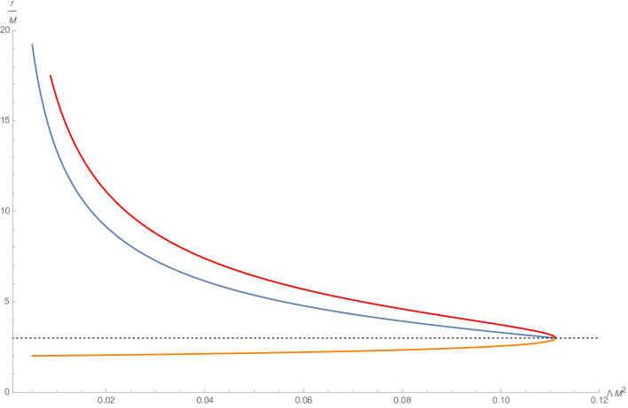
Figure 1: In this Figure, the wormhole throat $a_{0}$ is represented by the solid blue line which falls between the event horizon $r_{h}$ (orange) and the cosmological horizon $r_{c}$ (red) for all $\Lambda M^{2}<1/9$. We note that $\Lambda M^{2}=1/9$ is the extremal limit where both horizons degenerate into one and all $r_{c},r_{h},a_{0}\rightarrow 3M$. This point is excluded from our wormhole construction domain. Also, we note that the $\Lambda=0$ limit is singular.

Thus, we see that contrary to the Schwarzschild case, the regularity constraint $[K]=0$ is compatible with the wormhole construction procedure of identifying exteriors of the Schwarzschild-de Sitter spacetime. For this class of thin-shell wormholes, we find that the energy density $\sigma$ is unfortunately negative definite if we also adopt the unitarity constraint $1+2\beta R_{0}>0$ (see for e.g. [40]). For the weak energy condition to be obeyed, we require the coupling parameter $\beta$ to satisfy

$$1+\beta\left(2R_{0}-[K^{t}_{t}]^{2}\right)\leq 0.$$ (5.13)

We find that $2R_{0}-[K^{t}_{t}]^{2}$ is positive definite for $\Lambda M^{2}<1/9$, and that there is no negative $\beta$ which satisfies both (5.13) and the unitarity condition $1+2\beta R_{0}>0$. This implies that the family of Schwarzschild-de Sitter wormholes constructed here has to be supported by exotic matter at the throat. They are also unstable under radial perturbation.

5.2 Implications for stellar models

In the absence of a singular source, the generalized junction equations reduce to a set of conditions for the geometry induced by a non-singular energy-momentum tensor that is possibly discontinuous at $\Sigma$. In the ordinary Einstein theory, this simply translates to continuity in the extrinsic curvature, but taking $S_{\mu\nu}=0$ in the generalized junction conditions typically implies more complicated smoothness conditions on the extrinsic curvature.

In this Section, we briefly discuss the form of the junction conditions when the source is non-singular, and some implications for the $R+\beta R^{2}$ theory. In this case, it turns out to be convenient to begin by first setting $S_{in}=0$, which implies that

$$[R]=R_{0},$$ (5.14)

where $R_{0}$ is some constant. In the following, we classify the junction conditions according to whether $R_{0}$ is zero.

1. $[R]=0$:

   From the vanishing of $S_{ij}$, we have

   $$2\beta g_{ij}n^{\alpha}[\nabla_{\alpha}R]+[K_{ij}]\left(\frac{2\beta}{3}\left([K^{ab}][K_{ab}]-3R\right)-1\right)=0.$$

   Taking the trace implies that $n^{\alpha}[\nabla_{\alpha}R]=0$ together with the junction conditions

   $$[K_{ij}]=0,\qquad\text{or}\,\,\,\,\,\,[K^{ab}][K_{ab}]-3R=\frac{3}{2\beta}.$$ (5.15)

2. $[R]=R_{0}\neq 0$:

   In this case, $S_{nn}=0$ implies that $K=0$ and from the vanishing of $S_{ij}$, we have $n^{\alpha}[\nabla_{\alpha}R]=0$ together with the junction conditions

   $$[K_{ij}]\left(\frac{2\beta}{3}\left([K^{ab}][K_{ab}]-3\overline{R}\right)-1\right)=6\beta R_{0}\overline{K}_{ij}.$$ (5.16)

Generally, if $\Sigma$ is embedded in the bulk with the extrinsic and intrinsic curvature parametrically independent of $\beta$, then the junction conditions for cases (I) and (II) reduce to $n^{\alpha}[\nabla_{\alpha}R]=0$, and

$$[R]=[K_{ij}]=0,\qquad\text{or}\,\,\,\,\,\,\,[R]=R_{0}\neq 0,\,\,\,K_{ij}=0.$$ (5.17)

As an application, let’s apply (5.17) to a well-known family of line elements which model static stars with spherical symmetry. In ordinary GR, this class of solutions is constructed by matching a Schwarzschild exterior to a perfect fluid interior with metric of the form

$$ds^{2}_{int}=-A(r)dt^{2}+B^{-1}(r)dr^{2}+r^{2}(d\theta^{2}+\sin^{2}\theta d\phi^{2}),$$ (5.18)

where

$$A(r)=e^{2\alpha(r)},\,\,\,B(r)=1-\frac{2m(r)}{r},\,\,\,\alpha^{\prime}(r)=\frac{m(r)+4\pi r^{3}p(r)}{r(r-2m(r))},$$ (5.19)

which solves the field equations with the energy-momentum tensor of a perfect fluid

$$T_{\mu\nu}=(\rho(r)+p(r))U_{\mu}U_{\nu}+p(r)g_{\mu\nu},\,\,\,U_{\mu}=(\sqrt{A},0,0,0),$$ (5.20)

with the Tolman-Oppenheimer-Volkoff equation

$$p^{\prime}(r)=-\frac{m(r)}{r^{2}}\rho(r)\left(1+\frac{p(r)}{\rho(r)}\right)\left(1+\frac{4\pi r^{3}p(r)}{m}\right)\left(1-\frac{2m(r)}{r}\right)^{-1}.$$ (5.21)

The Schwarzschild solution is still a vacuum solution in $\mathcal{F}(R)=R+\beta R^{2}$ theory, and we also take the same interior solution as defined above but now this is sourced by a different energy-momentum which is the sum of (5.20) and extra terms arising from the field equations of the $\mathcal{F}(R)$ theory.

The surface $\Sigma$ is the star’s boundary defined by $r=R_{s}$ for some constant $R_{s}$ (which typically satisfies an appropriate Buchdahl bound). At $\Sigma$, imposing metric continuity and $[K_{ij}]=0$ lead to the boundary conditions

$$m(R_{s})=M,\,\,\,p(R_{s})=0,$$

where $M$ is the mass parameter of the Schwarzschild exterior. Note that for the metric of the form (5.18), the components of the extrinsic curvature are $K^{t}_{t}=\frac{1}{2}\frac{\sqrt{B}A^{\prime}}{A},K^{\theta}_{\theta}=K^{\phi}_{\phi}=\frac{\sqrt{B}}{R_{s}}$. Thus, matching it to a Schwarzschild exterior leads to $p(R_{s})=0$ after using (5.19). Since $R=-8\pi T^{\mu}_{\mu}=8\pi(\rho-3p)$, the additional junction conditions $[R]=0,[\partial_{r}R]=0$ further impose the additional boundary conditions

$$\rho(R_{s})=0,\,\,\,p^{\prime}(R_{s})=0,\,\,\,\rho^{\prime}(R_{s})=0.$$ (5.22)

For a polytropic equation of state of the form $p\propto\rho^{\gamma}$ for some positive constant $\gamma$, these boundary conditions are only compatible with the case of radiative matter $p=\frac{1}{3}\rho$. These results were similarly presented in [41] albeit through a different set of junction conditions. For the Tolman-Oppenheimer-Volkoff stellar model above, our junction conditions lead to an identical final set of boundary conditions on the interior fluid’s density and pressure.

Another well-studied stellar model that is also a cut-and-paste solution involving a Schwarzschild exterior is the Oppenheimer-Snyder solution where the interior is a closed FRW universe sourced by a pressureless dust. For this model of stellar formation, the matching surface $\Sigma$ is taken to preserve the $SO(3)$ isometry, and is comoving with the FRW interior of which metric reads

$$ds^{2}=a^{2}(\tau)\left(-d\tau^{2}+dR^{2}+\sin^{2}R(d\theta^{2}+\sin^{2}\theta d\phi^{2})\right).$$ (5.23)

The surface $\Sigma$ is defined as the sphere $R=R_{c}$ for some constant $R_{c}$, or in the coordinates of the Schwarzschild exterior, $r(\tau)=a(\tau)\sin(R_{c})$, with the scale factor $a(\tau)$ satisfying the Friedmann equations for a pressureless dust. It is straightforward to see that this solution is incompatible with the junction conditions (5.17) since the Ricci scalar $R=8\pi\rho$.

These simple examples appear to indicate that an embedding of GR solutions with discontinuous but non-singular sources is subject to rather stringent constraints associated with the generalized junction conditions in $F(R)$ theory. It is however important to note that we have examined only the simplest embedding, retaining the full GR metric and the geometry of $\Sigma$. The caveat is that this implies that the interior is sourced by an energy-momentum tensor of the form

$$T_{\mu\nu}=T^{(GR)}_{\mu\nu}+\frac{\beta}{4\pi}\left((g_{\mu\nu}\Box-\nabla_{\nu}\nabla_{\mu})R+RR_{\mu\nu}-\frac{1}{4}R^{2}g_{\mu\nu}\right).$$

It would be interesting to consider stellar models where $T_{\mu\nu}$ inherits a more physically motivated form, as well as other shapes of $\Sigma$ which may be dependent on various theory couplings in the $F(R)$ theory. This would probe a much wider landscape of solutions compatible with our generalized junction conditions.

6 Concluding Remarks

We have presented a general method to derive the appropriate Darmois-Israel junction conditions for gravitational theories with higher-order derivative terms by integrating the bulk equations of motion across the infinitesimal width of the singular hypersurface $\Sigma$ as defined in (2.5). A salient feature of our work is the presence of regularity constraints which impose conditions on the extrinsic curvature such that the integral in (2.5) converges. Geometrically, they specify the conditions under which the embedding of $\Sigma$ into the bulk spacetime is compatible with the delta-singular source localized within $\Sigma$.

Our method fundamentally relies on defining the $\delta$-distribution as the limit of a sequence of classical functions as expressed in (2.19) and (2.20). We found that the use of delta-convergent sequences yields a powerful language for organizing various terms with different orders of singularities appearing in the integral (2.5), and is intimately related to the procedure of Hadamard regularization commonly invoked in the theory of distributions. Upon imposing the regularity constraints, the integral in (2.5) converges and is well-defined. Our method passes a stringent consistency test (that is noticeably absent in previous literature) : that the junction conditions for Gauss-Bonnet gravity can be obtained as a suitable limit of those of quadratic gravity when the coupling constants reduce to those of the 4D Euler density term. This is a rigorous check of validity since the junction conditions for Gauss-Bonnet gravity can also be independently derived by boundary variation of a suitable surface term in the action.

As explicit examples of our approach, we demonstrated in detail how to obtain the regularity constraints and junction conditions for (i) quadratic gravity (ii) $\mathcal{F}(R)$ theories (iii) a 4D low-energy effective action in string theory and (iv) Euler density action terms which are higher-dimensional analogues of the 4D Gauss-Bonnet term. We have expressed these generalized junction conditions explicitly as functions of the extrinsic curvature tensor and its derivatives. Generically, they also involve components that are non-parallel to $\Sigma$, in contrast to the case in ordinary GR. To our knowledge, all of these generalized junction conditions are novel results. Although there have been past attempts to derive junction conditions for quadratic gravity [16] and $\mathcal{F}(R)$ theories [17, 13, 14], their results or underlying methodologies did not appear to demonstrate consistency with the Gauss-Bonnet case. In this aspect, we hope that our work has also clarified some of the ambiguities encountered in these previous studies.

The details of our derivation procedure presented here should be pedagogically useful towards adopting our methodology to derive junction conditions for other more complicated gravitational theories, including those with matter and gauge couplings. We should also mention that although our method applies rather widely to gravitational actions built out of curvature invariants, by definition, it does not apply to topological boundary terms in the action since they do not manifestly modify the bulk equations of motion. In an upcoming work [47], we derive and examine the generalized junction conditions for Chern-Pontryagin density terms by boundary variation of suitable surface terms. This class of theories includes, in particular, the (non-dynamical) ‘Chern-Simons gravity’ theory in 4D of which surface term was derived in [35].

We hope that these junction equations will furnish the essential first steps towards exploring a potentially rich and phenomenologically interesting landscape of classical solutions which have singular hypersurfaces as their defining geometric feature. In this work, we have briefly touched upon a couple of applications in the $\mathcal{F}(R)=R+\beta R^{2}$ theory, where we found a thin-shell wormhole constructed by identifying the exterior regions of two identical copies of Schwarzschild-de Sitter spacetime. We showed that many stellar models in ordinary GR which are lifted directly to this particular $\mathcal{F}(R)$ theory violate its regularity constraints. It would be very interesting to carry out a more extensive exploration of thin-shell and stellar geometries in many gravitational theories beyond GR, now that we are freshly equipped with the fundamental junction conditions to work with. In particular, we note that thin-shell wormholes have been recently revisited as black hole mimickers for LIGO events [48].

Another natural avenue for future work lies in extending our approach to cover $\Sigma$ which is lightlike. In this case, there is no unique definition of the extrinsic curvature once the induced metric on the surface becomes degenerate, since the normal vector defined in the setting of timelike/spacetlike $\Sigma$ is then tangent to $\Sigma$, and naively we need another notion of a ‘transverse’ vector. This subtle point has been addressed in [49] where a proposal for junction conditions in the case of a null surface was presented. It would be interesting to generalize the results of [49] to higher-derivative gravitational theories, and see if some aspects of our method remain useful.

Appendix A Some useful integral identities

In this Appendix, we collect a set of integral identities (i)—(v) which involve products of discontinuous functions and their derivatives. This accompanies the detailed derivation in Section 3 . The scaling limit (2.27) is implicitly taken for each final expression throughout this Section. When the argument of a function is omitted, it is understood to be evaluated at $n=0$.

$$\text{(i)}I_{1} = \int^{\epsilon}_{-\epsilon}dn\,\,\,f(n)\partial^{2}_{n}g(n)$$ (A.1)

$$= \int^{\epsilon}_{-\epsilon}dn\left(f_{1}(n)+\Theta(n,b)(f_{2}(n)-f_{1}(n))\right)\partial^{2}_{n}\left(g_{1}(n)+\Theta(n,b)(g_{2}(n)-g_{1}(n))\right)$$ (A.2)

$$= \frac{1}{2}(f_{1}(0)+f_{2}(0))[g^{\prime}_{2}(0)-g^{\prime}_{1}(0)]-\frac{1}{2}(g_{1}(0)+g_{2}(0))[f^{\prime}_{2}(0)-f^{\prime}_{1}(0)]$$ (A.4)

$$-\int^{\epsilon}_{-\epsilon}dn\,\,\,(f_{2}(n)-f_{1}(n))(g_{2}(n)-g_{1}(n))\left(\Theta^{\prime}(n,b)\right)^{2}$$

$$\equiv \overline{f}[g^{\prime}]-\overline{f}^{\prime}[g]-\int^{\epsilon}_{-\epsilon}dn\,\,\,[f(n)][g(n)]\left(\Theta^{\prime}(n,b)\right)^{2}$$ (A.5)

$$\text{(ii)}I_{2} = \int^{\epsilon}_{-\epsilon}dn\,\,\,\partial_{n}f(n)\partial_{n}g(n)$$ (A.6)

$$= \int^{\epsilon}_{-\epsilon}dn\left(f_{1}(n)+\Theta(n,b)(f_{2}(n)-f_{1}(n))\right)^{\prime}\left(g_{1}(n)+\Theta(n,b)(g_{2}(n)-g_{1}(n))\right)^{\prime}$$ (A.7)

$$= \overline{g}^{\prime}[f]+\overline{f}^{\prime}[g]+\int^{\epsilon}_{-\epsilon}dn\,\,\,[f(n)][g(n)]\left(\Theta^{\prime}(n,b)\right)^{2}.$$ (A.8)

In both $I_{1},I_{2}$, the singular parts of the integral may only arise in the term

$$I_{div}\equiv\int^{\epsilon}_{-\epsilon}dn\,\,\,[f(n)][g(n)]\left(\Theta^{\prime}(n,a)\right)^{2}=\lim_{b\rightarrow 0}\frac{1}{b}[f(0)][g(0)]\int^{\infty}_{-\infty}dX\,\,\,F^{2}(X),$$ (A.9)

where we have expanded $[f(n)][g(n)]$ around the origin, and restored the vanishing limit symbol for parameter $b$ to indicate the term’s singular nature. This is a particular case of the general formula we develop in (2.39), with $\sum_{m}k_{m}=2$ and thus $l=0$ is the only singular mode. In applying this integral identity to the junction equations, we note that we have to collect all singular terms that similarly diverge as $1/b$ and set the coefficient (which is typically a function of the extrinsic curvature and its derivatives) to vanish. One can similarly simplify integrals of the form

$$\int^{\epsilon}_{-\epsilon}dn\,\,\,\partial_{k_{1}}f_{1}\,\partial_{k_{2}}f_{2}\,\ldots\partial_{k_{r}}f_{r},$$ (A.10)

where $f_{1},f_{2},\ldots,f_{r}$ are discontinuous functions. After expanding various functions (apart from $\delta_{b}(n)$ and its derivatives) about the origin, we then obtain a linear combination of (2.39). Only a finite number of terms remain, including the singular terms. As an another example, let’s consider

$$I_{3}=\int^{\epsilon}_{-\epsilon}f(n)\partial^{3}_{n}g(n).$$

After some similar manipulations as in the previous examples, we obtain

$$\text{(iii)}I_{3} = [fg^{\prime\prime}]-[f]\overline{g}^{\prime\prime}-\overline{f}^{\prime}[g^{\prime}]+\overline{f}^{\prime\prime}[g]$$ (A.12)

$$+\int^{\epsilon}_{-\epsilon}dn\,\,\,(\Theta^{\prime}(n,b))^{2}\left(2[f(n)][g^{\prime}(n)]-[f^{\prime}(n)][g(n)]\right)+\Theta^{\prime}(n,b)\Theta^{\prime\prime}(n,b)[f(n)][g(n)]$$

$$= [fg^{\prime\prime}]-[f]\overline{g}^{\prime\prime}-\overline{f}^{\prime}[g^{\prime}]+\overline{f}^{\prime\prime}[g]-\lim_{b\rightarrow 0}\frac{3}{2b}\left([f][g^{\prime}]-[f^{\prime}][g]\right)\int^{\infty}_{-\infty}dXF^{2}(X)$$ (A.13)

Again, we see that there is one singular term that diverges as $1/b$.

Another useful formula that we will need is

$$\text{(iv)}I_{4}=\int^{\epsilon}_{-\epsilon}dn\,\,\,f(n)g(n)\partial_{n}h(n)=\frac{1}{3}\left(\overline{fg}+2\overline{f}\overline{g}\right)[h]\equiv\overbracket{fg}[h],$$ (A.14)

where the various functions are all discontinuous at $n=0$ in the limit $\epsilon\rightarrow 0$, and we have taken the liberty to introduce a bold overline for notational simplicity since as we shall see, such combination of averaging over functions (of extrinsic curvature) occurs frequently in the junction equations for gravitational theories with Lagrangian terms that are quadratic invariants of the Riemann tensor. To obtain (A.14), we simply note that the LHS is equivalently

$$\int^{\epsilon}_{-\epsilon}dn\,\,\,\left(f_{1}(n)+\Theta(n)(f_{2}(n)-f_{1}(n))\right)\left(g_{1}(n)+\Theta(n)(g_{2}(n)-g_{1}(n))\right)\Theta^{\prime}(n)\left(h_{2}(n)-h_{1}(n)\right),$$ (A.15)

with all functions being continuous. Upon using the identity $\int dn\,\,\Theta^{\prime}(n)\Theta^{k}(n)F(n)=\frac{1}{k+1}F(0)$, we are then led to (A.14).

Finally, another useful integral which we will encounter in deriving junction equations for gravitational Lagrangians with quadratic invariants is

$$\text{(v)}I_{5} = \int^{\epsilon}_{-\epsilon}dn\,\,g_{ij}\partial_{n}f\partial_{n}h$$

$$= g_{ij}\overline{f^{\prime}}[h]+\overline{h^{\prime}}[f]g_{ij}+\lim_{b\rightarrow 0}\frac{1}{b}g_{ij}[h][f]\int^{\infty}_{-\infty}dX\,F^{2}(X)+2[f][h][g^{\prime}_{ij}]\int^{\infty}_{0}dX\,XF^{2}(X).$$

We note that there is a singular term arising from this integral and another finite term that is depends on the choice of the nascent delta function. This can be interpreted as an (infinite) sum of various moments of $\delta_{b}(X)$ after expanding $\Theta(bX,b)$ and a factor of $F(X)$ in $X$. Since the coefficient is of the same form as the singular term (apart from replacing $g_{ij}$ with its normal derivative), we will find that this representation-dependent term naturally cancels out when we impose the regularity condition.

To arrive at (A), we can apply the same techniques that we used in proving the previous integral identities, taking into account that we take $g_{ij}$ to be generally non-differentiable. As a consistency check, let us write the integrand in the LHS of (A) as

$$g_{ij}\partial_{n}f\partial_{n}h=\partial_{n}(g_{ij}f)\partial_{n}h-(\partial_{n}g_{ij})f\partial_{n}h,$$ (A.17)

and similar to how we obtain $I_{2}$ in (A.6), it is straightforward to obtain

$$\int^{\epsilon}_{-\epsilon}dn\,\,\partial_{n}(g_{ij}f)\partial_{n}h = g_{ij}\overline{f^{\prime}}[h]+\overline{h^{\prime}}[f]g_{ij}+\lim_{b\rightarrow 0}\frac{1}{b}g_{ij}[h][f]\int^{\infty}_{-\infty}dX\,\,F^{2}(X)$$

$$+2[f][h][g^{\prime}_{ij}]\int^{\infty}_{0}dX\,XF^{2}(X)$$

$$\qquad+\left((\overline{g^{\prime}_{ij}}-\frac{1}{2}[g^{\prime}_{ij}])[h]\overline{f}+\frac{1}{2}[h][g^{\prime}_{ij}](\overline{f}-\frac{1}{2}[f])+\frac{1}{3}[g^{\prime}_{ij}][f][h]\right).$$

After some algebra, one can show that the last line (in brackets) of (A) is precisely $\int^{\epsilon}_{-\epsilon}dn\,f\partial_{n}g_{ij}\partial_{n}h$ after using the identity (A.14), and thus furnishing a nice consistency check between (A) and (A.14).

Appendix B From quadratic gravity to Gauss-Bonnet theory: some notes on the junction conditions

We have seen that for the Gauss-Bonnet theory, there are no additional constraints on the extrinsic curvature that we have to impose for regularity. Let us now elaborate on a subtlety arising in this topological limit.

For the case of Gauss-Bonnet gravity, the junction conditions were derived in [36] via a bulk integration across $\Sigma$. An alternate derivation was performed in [24] via the boundary variation of an appropriate surface term that appeared earlier in [26] — a seminal work where surface terms for higher-dimensional topological Euler density terms were also derived. These surface terms are required for a well-defined action principle with Dirichlet conditions. As explained in [26], the Euler density terms $\chi_{2m}$ that one can define in every even dimension $2m$ are precisely the linear combination of curvature invariants that generate only second-order field equations, and thus, in principle, these exists appropriate surface terms for them. The simplest example would be the Ricci scalar $\chi_{2}$ being the Euler density in two dimensions. The surface term for $\chi_{2}$ is the Gibbons-Hawking-York term $S_{GHY}=\frac{1}{8\pi}\int d^{d-1}x\,\,\sqrt{h}K$. This continues to hold for dimensions $>2$, and hence the junction conditions (1.1), even when the theory itself is no longer topological in dimensions $>2$. Similarly, the Gauss-Bonnet term $\chi_{4}$ is the topological Euler density term in 4D, trivial in lower dimensions and non-topological in dimensions $>4$. Adding it to the Einstein-Hilbert action yields additional junction terms which are third-order polynomials in the extrinsic curvature [36, 24]. For junction terms descending from a boundary variation of surface terms, since the normal vector to $\Sigma$ points in opposite directions when we take $\Sigma$ to bound the spacetime region on each side, this naturally leads to junction terms which are expressible in terms of bracketed quantities like (1.1).

As already argued in [26, 27] and definitively shown in [28], the equations of motion of a generic higher-derivative gravitational theory do not descend from a well-posed variational principle with Dirichlet conditions. Hence, the approach of obtaining their junction conditions by boundary variation of surface terms is not applicable, since an appropriate surface term does not exist for a generic higher-derivative theory. On this point, we note that a recent work [17] claimed to have derived the junction conditions for quadratic gravity by using the variational principle. However, in their derivation, they imposed a form (eqn. 62 in [17]) for the variation of the extrinsic curvature that is problematic, and does not follow consistently from its fundamental definition (for the interested reader, see e.g. [24, 35] for the correct expression for $\delta K_{ij}$.)

Nonetheless, the junction conditions for the Euler-density terms can serve as vigorous consistency checks for those belonging to gravitational theories of which action is constructed from some linear combination of curvature invariants including those defining $\chi_{2m}$. Varying the action with the Gauss-Bonnet term

$$\mathcal{L}_{GB}=R+\beta_{1}\left(R^{2}-4R_{\alpha\beta}R^{\alpha\beta}+R^{\alpha\beta\mu\nu}R_{\alpha\beta\mu\nu}\right),$$

with respect to the metric yields the following the equation of motion

$$\frac{\delta\mathcal{L}}{\delta g^{\alpha\beta}} = G_{\alpha\beta}+2\beta_{1}\left(RR_{\alpha\beta}-2R_{\alpha\mu}{R^{\mu}}_{\beta}-2R^{\mu\nu}R_{\alpha\mu\beta\nu}+{R_{\alpha}}^{\mu\nu\chi}R_{\beta\mu\nu\chi}\right)$$ (B.1)

$$\quad-\frac{\beta_{1}}{2}g_{\alpha\beta}\left(R^{2}-4R_{\alpha\beta}R^{\alpha\beta}+R^{\alpha\beta\mu\nu}R_{\alpha\beta\mu\nu}\right).$$

We now proceed to verify that taking $\beta_{2}=-4\beta_{3}=-4\beta_{1}$ in $\tilde{G}_{ij}$ yields exactly the same junction conditions derived from the method of boundary variation. This furnishes a strong consistency check of many expressions in the previous Section (explicitly, they are equations (3.8), (3.13), (3.17), (3.21), (3.23), (3.25) and (3.28)).

In the following, we focus on the part in (B.1) that is coupled to $\beta_{1}$ which we suppress for the workings below for notational simplicity. Consider first all terms involving the intrinsic curvature of $\Sigma$ which are various contractions of products of $\hat{R}_{abcd}$, the extrinsic curvature tensor and the metric tensor. After some algebra, we find that they sum up to read

$$2\left(-2\hat{R}_{ij}[K]+2\hat{R}_{m(j}K^{m}_{i)}+2[K^{ab}]\hat{R}_{iajb}-\hat{R}[K_{ij}]\right)-4g_{ij}\left(\hat{R}_{cd}[K^{cd}]-\frac{1}{2}\hat{R}[K]\right),$$ (B.2)

which can be written as $-4P_{icdj}[K^{cd}]$ with $P_{icdj}$ being the divergence-free part of the Riemann curvature tensor of $\Sigma$ as defined in (3.79) earlier.

Next, we consider all terms that contain a factor of the induced metric $g_{ij}$ which sum up to read

$$-\frac{1}{2}g_{ij}\left(4[K]\overbracket{K^{2}}-4[K]\overbracket{K^{ab}K_{ab}}-8\overbracket{KK^{ab}}[K_{ab}]+8\overbracket{K^{b}_{l}K^{la}}[K_{ab}]\right)$$ (B.3)

Expressing all quantities in (B.3) in terms of the ordinary averaging symbol, and using the fact that

$$[K^{m}_{l}K^{la}K_{ma}] = \overline{K^{m}_{l}K^{la}}[K_{ma}]+[K^{m}_{l}K^{la}]\overline{K_{ma}}=\overline{K^{m}_{l}K^{la}}[K_{ma}]+2\overline{K^{m}_{l}}\overline{K^{la}}[K_{ma}],$$ (B.4)

$$[KK^{ab}K_{ab}] = [K]\overline{K^{ab}K_{ab}}+[K^{ab}K_{ab}]\overline{K}=[K]\overline{K^{ab}K_{ab}}+2\overline{K^{ab}}\overline{K}[K_{ab}],$$ (B.5)

$$[KK^{ab}K_{ab}] = \overline{KK^{ab}}[K_{ab}]+[KK_{ab}]\overline{K_{ab}}=\overline{KK^{ab}}[K_{ab}]+\overline{K}\overline{K^{ab}}[K_{ab}]+[K]\overline{K^{ab}}\overline{K_{ab}},$$ (B.6)

one can straightforwardly show that (B.3) can be expressed purely in terms of commutators and read as

$$-\frac{1}{2}g_{ij}\frac{4}{3}\left([K^{3}]-3[KK^{ab}K_{ab}]+2[K_{l}^{m}K^{la}K_{ma}]\right)$$ (B.7)

Finally, let’s consider all other terms. For those involving $K_{ij}K^{2}$, they arise from (3.21) and can be simplified as

$$2\left(2\overbracket{KK_{ij}}[K]+\overbracket{K^{2}}[K_{ij}]\right)=\frac{4}{3}\left(\overline{KK_{ij}}+2\overline{K}\,\overline{K_{ij}}\right)[K]+\frac{2}{3}(\overline{K^{2}}+2\overline{K}^{2})[K_{ij}]$$ (B.8)

By noting that

$$[K_{ij}K^{2}] = \overline{K_{ij}K}[K]+[K_{ij}K]\overline{K}=\overline{K_{ij}K}[K]+\overline{K_{ij}}\,\overline{K}[K]+\overline{K}^{2}[K_{ij}],$$ (B.9)

$$= \overline{K^{2}}[K_{ij}]+[K^{2}]\overline{K_{ij}}=\overline{K^{2}}[K_{ij}]+2[K]\overline{K}\,\overline{K_{ij}}$$ (B.10)

some straightforward algebra then leads one to see that (B.8) can be written purely in terms of a bracket and reads

$$2\left(2\overbracket{KK_{ij}}[K]+\overbracket{K^{2}}[K_{ij}]\right)=2[K_{ij}K^{2}]$$ (B.11)

Next, we consider terms of the form $K_{ij}K^{ab}K_{ab}$ which arise from (3.21) and (3.28). They sum up to read

$$-2\left(\overbracket{K^{ab}K_{ab}}[K_{ij}]+2\overbracket{K_{ij}K^{ab}}[K_{ab}]\right)=-2\left([K_{ij}K_{ab}K^{ab}]\right)$$ (B.12)

where we have invoked identities similar to the form of (B.6). Thus, all terms containing a factor of $K_{ij}$ sum up to be a single bracket of the form

$$2\left[K_{ij}(K^{2}-K_{ab}K^{ab})\right]$$ (B.13)

Next, we consider terms of the form $K_{ja}K_{ib}K^{ab}$ which arise in (3.23), (3.25) and (3.28). They sum up to read

$$2\left(2\overbracket{K^{l}_{m}K_{l(i}}[K_{j)}^{m}]+[K^{l}_{m}]\overbracket{K_{l(j}K^{m}_{i)}}\right)=2[K^{l}_{m}K_{l(j}K^{m}_{i)}]$$ (B.14)

where again we have invoked identities similar to the form of (B.6). Finally, we are left with terms of the form $KK_{ia}K^{a}_{j}$. They arise in (3.21), (3.23) and (3.28), and sum up to read

$$-2\left(\overbracket{K_{m(j}K^{m}_{i)}}[K]+2\overbracket{KK_{m(j}}[K^{m}_{i)}]\right)=-2[K_{m(j}K^{m}_{i)}K].$$ (B.15)

Gathering all terms together, and including the Gibbons-Hawking terms from Einstein-Hilbert action, we find the junction condition to be

$$[K]h_{ij}-[K_{ij}]-2\beta_{1}\left[(3J_{ij}-Jh_{ij}+2P_{icdj}K^{cd})\right]=8\pi S_{ij},$$ (B.16)

where $P_{icdj}$ is the divergence free part of the Riemann tensor and $J_{ij}=\frac{1}{3}(2KK_{ic}K^{c}_{j}+K_{cd}K^{cd}K_{ij}-2K_{ic}K^{cd}K_{dj}-K^{2}K_{ij})$. This is identical to the junction condition derived in earlier literature [26, 24, 25, 36] via boundary variation.

References

- [1] G. Darmois, “Les equations de la gravitation einsteinienne,” Memorial de Sciences Mathematiques, Fascicule XXV (1927)
- [2] W. Israel, “Singular Hypersurfaces and Thin Shells in General Relativity,” Nuovo Cimento (10), 44B: 1-14 (1966)
- [3] C. Lanczos, Phys. Zeits., 23, 539 (1922); Ann. der Phys., 74, 518 (1924). See also N. Sen: Ann. der Phys., 73 365 (1924).
- [4] G. W. Gibbons and S. W. Hawking, “Action Integrals and Partition Functions in Quantum Gravity,” Phys. Rev. D 15, 2752-2756 (1977) doi:10.1103/PhysRevD.15.2752
- [5] J. W. York, Jr., “Conformatlly invariant orthogonal decomposition of symmetric tensors on Riemannian manifolds and the initial value problem of general relativity,” J. Math. Phys. 14, 456-464 (1973) doi:10.1063/1.1666338
- [6] E. Poisson and M. Visser, “Thin shell wormholes: Linearization stability,” Phys. Rev. D 52, 7318-7321 (1995) doi:10.1103/PhysRevD.52.7318 [arXiv:gr-qc/9506083 [gr-qc]].
- [7] P. O. Mazur and E. Mottola, “Gravitational condensate stars: An alternative to black holes,” [arXiv:gr-qc/0109035 [gr-qc]].
- [8] N. Uchikata and S. Yoshida, “Slowly rotating thin shell gravastars,” Class. Quant. Grav. 33, no.2, 025005 (2016) doi:10.1088/0264-9381/33/2/025005 [arXiv:1506.06485 [gr-qc]].
- [9] F. Fayos, X. Jaén, E. Llanta and J. M. Senovilla, “Interiors of Vaidya’s radiating metric: Gravitational collapse,” Phys. Rev. D 45 2732-2738 (1992) doi: 10.1103/physrevd.45.2732.
- [10] F. Fayos, J. M. Senovilla and R. Torres, “General matching of two spherically symmetric space-times,” Phys. Rev. D 54, 4862-4872 (1996) doi:10.1103/PhysRevD.54.4862
- [11] J. R. Oppenheimer and H. Snyder, “On Continued gravitational contraction,” Phys. Rev. 56, 455-459 (1939) doi:10.1103/PhysRev.56.455
- [12] S. K. Blau, E. I. Guendelman and A. H. Guth, “The Dynamics of False Vacuum Bubbles,” Phys. Rev. D 35, 1747 (1987) doi:10.1103/PhysRevD.35.1747
- [13] J. Senovilla, M.M., “Junction conditions for F(R)-gravity and their consequences,” Phys. Rev. D 88, 064015 (2013) doi:10.1103/PhysRevD.88.064015 [arXiv:1303.1408 [gr-qc]].
- [14] N. Deruelle, M. Sasaki and Y. Sendouda, “Junction conditions in f(R) theories of gravity,” Prog. Theor. Phys. 119, 237-251 (2008) doi:10.1143/PTP.119.237 [arXiv:0711.1150 [gr-qc]].
- [15] G. J. Olmo and D. Rubiera-Garcia, “Junction conditions in Palatini gravity,” [arXiv:2007.04065 [gr-qc]].
- [16] B. Reina, J. M. M. Senovilla and R. Vera, “Junction conditions in quadratic gravity: thin shells and double layers,” Class. Quant. Grav. 33, no.10, 105008 (2016) doi:10.1088/0264-9381/33/10/105008 [arXiv:1510.05515 [gr-qc]].
- [17] V. A. Berezin, V. I. Dokuchaev, Y. N. Eroshenko and A. L. Smirnov, “Double layer from least action principle,” Class. Quant. Grav. 38, no.4, 045014 (2021) doi:10.1088/1361-6382/abd143 [arXiv:2008.01813 [gr-qc]].
- [18] M. Mars and J. M. M. Senovilla, “Geometry of general hypersurfaces in space-time: Junction conditions,” Class. Quant. Grav. 10, 1865-1897 (1993) doi:10.1088/0264-9381/10/9/026 [arXiv:gr-qc/0201054 [gr-qc]].
- [19] J. Hadamard, “Lectures on Cauchy’s problem in linear partial differential equations,” Dover Phoenix editions, Dover Publications, New York (1923), “Le problème de Cauchy et les équations aux dérivées partielles linéaires hyperboliques,” Paris (1932).
- [20] P. K. Ram, “Generalized Functions — Theory and Applications,” Birkhauser Boston, New York (2004).
- [21] D. S. Jones, “Generalised functions,” McGraw-Hill, New York (1966).
- [22] J. M. M. Senovilla, “Gravitational double layers,” Class. Quant. Grav. 31, 072002 (2014) doi:10.1088/0264-9381/31/7/072002 [arXiv:1402.1139 [gr-qc]].
- [23] J. M. M. Senovilla, “Double layers in gravity theories,” J. Phys. Conf. Ser. 600, no.1, 012004 (2015) doi:10.1088/1742-6596/600/1/012004 [arXiv:1410.5650 [gr-qc]].
- [24] S. C. Davis, “Generalized Israel junction conditions for a Gauss-Bonnet brane world,” Phys. Rev. D 67, 024030 (2003) doi:10.1103/PhysRevD.67.024030 [arXiv:hep-th/0208205 [hep-th]].
- [25] E. Gravanis and S. Willison, “Israel conditions for the Gauss-Bonnet theory and the Friedmann equation on the brane universe,” Phys. Lett. B 562, 118-126 (2003) doi:10.1016/S0370-2693(03)00555-0 [arXiv:hep-th/0209076 [hep-th]].
- [26] R. C. Myers, “Higher Derivative Gravity, Surface Terms and String Theory,” Phys. Rev. D 36, 392 (1987) doi:10.1103/PhysRevD.36.392
- [27] M. S. Madsen and J. D. Barrow, “De Sitter Ground States and Boundary Terms in Generalized Gravity,” Nucl. Phys. B 323, 242-252 (1989) doi:10.1016/0550-3213(89)90596-8
- [28] J. Smolic and M. Taylor, “Higher derivative effects for 4d AdS gravity,” JHEP 06, 096 (2013) doi:10.1007/JHEP06(2013)096 [arXiv:1301.5205 [hep-th]].
- [29] M. J. Lighthill, “An introduction to Fourier analysis and generalised functions,” Cambridge University Press, London 1958.
- [30] A. I. Saichev and W. Woyczynski, “Distributions in the Physical and Engineering Sciences, Vol.1, Applied and Numerical Harmonic Analysis,” Springer Nature, Switzerland 2018.
- [31] L. Schwartz, “Theorie des Distributions,” Masson, Paris (1966).
- [32] I. M. Gel’fand and G. E. Shilov, “Generalized Functions,” Academic, New York (1964) Vol. 1, pp. 34-38.
- [33] J. M Aguirregabiria, A. Hernandez and M. Rivas, “-function converging sequences,” American Journal of Physics 70, 180-185 (2002) doi:10.1119/1.1427087
- [34] R. S. Strichartz, “A guide to distribution theory and fourier transforms,” World Scientific Publishing Co. Pte. Ltd. (2003).
- [35] D. Grumiller, R. B. Mann and R. McNees, “Dirichlet boundary value problem for Chern-Simons modified gravity,” Phys. Rev. D 78, 081502 (2008) doi:10.1103/PhysRevD.78.081502 [arXiv:0803.1485 [gr-qc]].
- [36] N. Deruelle and T. Dolezel, “Brane versus shell cosmologies in Einstein and Einstein-Gauss-Bonnet theories,” Phys. Rev. D 62, 103502 (2000) doi:10.1103/PhysRevD.62.103502 [arXiv:gr-qc/0004021 [gr-qc]].
- [37] J. Polchinski, “String theory. Vol. 2: Superstring theory and beyond,” doi:10.1017/CBO9780511618123
- [38] P. A. Cano and A. Ruipérez, “Leading higher-derivative corrections to Kerr geometry,” JHEP 05, 189 (2019) doi:10.1007/JHEP05(2019)189 [arXiv:1901.01315 [gr-qc]].
- [39] V. T. Gurovich and A. A. Starobinsky, Zh. Eksp. Teor. Fiz., 77 (1979), p. 1699
- [40] E. F. Eiroa and G. Figueroa Aguirre, “Thin-shell wormholes with charge in F(R) gravity,” Eur. Phys. J. C 76, no.3, 132 (2016) doi:10.1140/epjc/s10052-016-3984-1 [arXiv:1511.02806 [gr-qc]].
- [41] F. S. N. Lobo and M. A. Oliveira, “Wormhole geometries in f(R) modified theories of gravity,” Phys. Rev. D 80, 104012 (2009) doi:10.1103/PhysRevD.80.104012 [arXiv:0909.5539 [gr-qc]].
- [42] M. G. Richarte and C. Simeone, “Thin-shell wormholes supported by ordinary matter in Einstein-Gauss-Bonnet gravity,” Phys. Rev. D 76, 087502 (2007) [erratum: Phys. Rev. D 77, 089903 (2008)] doi:10.1103/PhysRevD.77.089903 [arXiv:0710.2041 [gr-qc]].
- [43] I. P. Lobo, M. G. Richarte, J. P. Morais Graça and H. Moradpour, “Thin-shell wormholes in Rastall gravity,” Eur. Phys. J. Plus 135, no.7, 550 (2020) doi:10.1140/epjp/s13360-020-00553-y [arXiv:2007.05641 [gr-qc]].
- [44] M. G. Richarte, I. G. Salako, J. P. Morais Graça, H. Moradpour and A. Övgün, “Relativistic Bose-Einstein condensates thin-shell wormholes,” Phys. Rev. D 96, no.8, 084022 (2017) doi:10.1103/PhysRevD.96.084022 [arXiv:1710.05886 [gr-qc]].
- [45] M. G. Richarte, “Wormholes and solitonic shells in five-dimensional DGP theory,” Phys. Rev. D 82, 044021 (2010) doi:10.1103/PhysRevD.82.044021 [arXiv:1003.0741 [gr-qc]].
- [46] E. F. Eiroa, M. G. Richarte and C. Simeone, “Thin-shell wormholes in Brans-Dicke gravity,” Phys. Lett. A 373, 1-4 (2008) [erratum: Phys. Lett. 373, 2399-2400 (2009)] doi:10.1016/j.physleta.2008.10.065 [arXiv:0809.1623 [gr-qc]].
- [47] C. S. Chu and H. .S. Tan, “Generalized junction conditions for gravitational Chern-Pontryagin invariants” Work in progress
- [48] V. Cardoso, E. Franzin and P. Pani, “Is the gravitational-wave ringdown a probe of the event horizon?,” Phys. Rev. Lett. 116, no.17, 171101 (2016) [erratum: Phys. Rev. Lett. 117, no.8, 089902 (2016)] doi:10.1103/PhysRevLett.116.171101 [arXiv:1602.07309 [gr-qc]].
- [49] C. Barrabes and W. Israel, “Thin shells in general relativity and cosmology: the lightlike limit,” Phys. Rev. D 43, 1129-1142 (1991)