Affine-Mapping based Variational Ensemble Kalman Filter

Abstract

We propose an affine-mapping based variational Ensemble Kalman filter for sequential Bayesian filtering problems with generic observation models. Specifically, the proposed method is formulated as to construct an affine mapping from the prior ensemble to the posterior one, and the affine mapping is computed via a variational Bayesian formulation, i.e., by minimizing the Kullback-Leibler divergence between the transformed distribution through the affine mapping and the actual posterior. Some theoretical properties of resulting optimization problem are studied and a gradient descent scheme is proposed to solve the resulting optimization problem. With numerical examples we demonstrate that the method has competitive performance against existing methods.

1 Introduction

The ensemble Kalman filter (EnKF) [14, 13] is one of the most popular tools for sequential data assimilation, thanks to its computational efficiency and flexibility [17, 34, 13]. Simply put, at each time step EnKF approximates the prior, the likelihood and the posterior by Gaussian distributions. Such a Gaussian approximation allows an affine update that maps the prior ensemble to the posterior one. This Gaussian approximation and the resulting affine update are the key that enables EnKF to handle large-scale problems with a relatively small number of ensembles. In the conventional EnKF, it is required that the observation model is Gaussian-linear, which means that the observation operator is linear and the noise is additive Gaussian. However, in many real-world applications, neither of these two requirements is satisfied. When the actual observation model is not Gaussian-linear, the EnKF method may suffer from substantial estimation error, which is discussed in details in Section 3.2. To the end, it is of practical importance to develop methods that can better deal with generic observation models than EnKF, while retaining the computational advantage (i.e., using a small ensemble size) of it.

A notable example of such methods is the nonlinear ensemble adjustment filter (NLEAF) [20], which involves a correction scheme: the posterior moments are calculated with importance sampling and the ensembles are then corrected accordingly. Other methods that can be applied to such problems include [2, 1, 18, 21, 6] (some of them may need certain modifications), just to name a few. In this work we focus on the EnKF type of methods that can use a small number of ensembles in high dimensional problems, and methods involving full Monte Carlo sampling such as the particle filter (PF) [4, 11] are not in our scope. It is also worth noting that a class of methods combine EnKF and PF to alleviate the estimation bias induced by the non-Gaussianity (e.g., [33, 16]), and typically the EnKF part in such methods still requires a Gaussian-linear observation model (or to be treated as such a model).

The main purpose of this work is to provide an alternative framework to implement EnKF for arbitrary observation models. Specifically, the proposed method formulates the EnKF update as to construct an affine mapping from the prior to the posterior and such an affine mapping is computed in variational Bayesian framework [25]. That is, we seek the affine mapping minimizing the Kullback-Leibler divergence (KLD) between the “transformed” prior distribution and the posterior. We note here that a similar formulation has been used in the variational (ensemble) Kalman filter [5, 32]. The difference is however, the variational (ensemble) Kalman filter methods mentioned above still rely on the linear-Gaussian observation model, where the variational formulation, combined with a BFGS scheme, is used to avoid the inversion and storage of very large matrices, while in our work the variational formulation is used to compute the optimal affine mapping for generic observation models.

It can be seen that this affine mapping based variational EnKF (VEnKF) reduces to the standard EnKF when the observation model is Gaussian-linear, and as such it is a natural generalization of the standard EnKF to generic observation models. Also, by design the obtained affine mapping is optimal under the variational (minimal KLD) principle. We also present a numerical scheme based on gradient descent algorithm to solve the resulting optimization problem, and with numerical examples we demonstrate that the method has competitive performance against several existing methods. Finally we emphasize that, though the proposed method can perform well for generic observation models, it requires the same assumption as the standard EnKF, i.e., the posterior distributions should not deviate significantly from Gaussian.

The rest of the work is organized as follows. In Section 2 we provide a generic formulation of the sequential Bayesian filtering problem. In Section 3 we present the proposed affine mapping based variational EnKF. Numerical examples are provided in Section 4 to demonstrate the performance of the proposed method and finally some closing remarks are offered in Section 5.

2 Problem Formulation

2.1 Hidden Markov Model

We start with the hidden Markov model (HMM), which is a generic formulation for data assimilation problems [11]. Specifically let $\{x_{t}\}_{t\geq 0}$ and $\{y_{t}\}_{t\geq 0}$ be two discrete-time stochastic processes, taking values from continuous state spaces $\mathcal{X}$ and $\mathcal{Y}$ respectively. Throughout this work we assume that $\mathcal{X}=\mathbb{R}^{n_{x}}$ and $\mathcal{Y}=\mathbb{R}^{n_{y}}$. The HMM model assumes that the pair $\{x_{t},y_{t}\}$ has the following property,

$$x_{t}|x_{1:t-1},y_{1:t-1} \sim \pi(x_{t}|x_{t-1}),\quad x_{0}\sim\pi(x_{0}),$$ (1a)

$$y_{t}|x_{1:t},y_{1:t-1} \sim \pi(y_{t}|x_{t}),$$ (1b)

where for simplicity we assume that the probability density functions (PDF) of all the distributions exist and $\pi(\cdot)$ is used as a generic notation of a PDF whose actual meaning is specified by its arguments.

In the HMM formulation, $\{x_{t}\}$ and $\{y_{t}\}$ are known respectively as the hidden and the observed states, and a schematic illustration of HMM is shown in Fig. 1. This framework represents many practical problems of interest [15, 19, 8], where one makes observations of $\{y_{t}\}_{t\geq 0}$ and wants to estimate the hidden states $\{x_{t}\}_{t\geq 0}$ therefrom. A typically example of HMM is the following stochastic discrete-time dynamical system:

$$x_{t} = F_{t}(x_{t-1},\alpha_{t}),\quad x_{0}\sim\pi(x_{0}),$$ (2a)

$$y_{t} = G_{t}(x_{t},\beta_{t}),$$ (2b)

where $\alpha_{t}\sim\pi^{\alpha}_{t}(\cdot)$ and $\beta_{t}\sim\pi^{\beta}_{t}(\cdot)$ are random variables representing respectively the model error and the observation noise at time $t$. In many real-world applications such as numerical weather prediction [7], Eq. (2a), which represents the underlying physical model, is computationally intensive, while Eq. (2b), describing the observation model, is often available analytically and therefore easy to evaluate. It follows that, in such problems, 1) one can only afford a small number of particles in the filtering, 2) Eq. (2a) accounts for the vast majority of the computational cost. All our numerical examples are described in this form and further details can be found in Section 4.

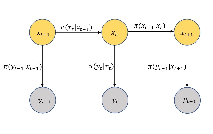
Figure 1: A schematic illustration of the Hidden Markov Model.

2.2 Recursive Bayesian Filtering

Recursive Bayesian filtering [10] is a popular framework to estimate the hidden states in a HMM, and it aims to compute the condition distribution $\pi(x_{t}|y_{1:t})$ for $t=1,2,\ldots$ recursively. In what follows we discuss how the recursive Bayesian filtering proceeds.

First applying the Bayes’ formula, we obtain

$$\pi(x_{t}|y_{1:t})=\frac{\pi(y_{t}|x_{t},y_{1:t-1})\pi(x_{t}|y_{1:t-1})}{\pi(y_{t}|y_{1:t-1})},$$ (3)

where $\pi(y_{t}|y_{1:t-1})$ is the normalization constant that often does not need to be evaluated in practice. From Eq. (1b) we know that $y_{t}$ is independent of $y_{t-1}$ conditionally on $x_{t}$, and thus Eq. (3) becomes

$$\pi(x_{t}|y_{1:t})=\frac{\pi(y_{t}|x_{t})\pi(x_{t}|y_{1:t-1})}{\pi(y_{t}|y_{1:t-1})}.$$ (4)

The condition distribution $\pi(x_{t}|y_{1:t-1})$ can be expressed as

$$\pi(x_{t}|y_{1:t-1})=\int\pi(x_{t}|x_{t-1},y_{1:t-1})\pi(x_{t-1}|y_{1:t-1})dx_{t-1},$$ (5)

and again thanks to the property of the HMM in Eq. (1), we have,

$$\pi(x_{t}|y_{1:t-1})=\int\pi(x_{t}|x_{t-1})\pi(x_{t-1}|y_{1:t-1})dx_{t-1},$$ (6)

where $\pi(x_{t-1}|y_{1:t-1})$ is the posterior distribution at the previous step $t-1$.

As a result the recursive Bayesian filtering performs the following two steps in each iteration:

• Prediction step: the prior density $\pi(x_{t}|y_{1:t-1})$ is determined via Eq. (6),

• Update step: the posterior density $\pi(x_{t}|y_{1:t})$ is computed via Eq. (4).

The recursive Bayesian filtering provides a generic framework for sequentially computing the conditional distribution $\pi(x_{t}|y_{1:t})$ as the iteration proceeds. In practice, the analytical expressions for the posterior $\pi(x_{t}|y_{1:t})$ or the prior $\pi(x_{t}|y_{1:t-1})$ usually can not be obtained, and therefore these distributions have to be represented numerically, for example, by an ensemble of particles.

3 Affine mapping based VEnKF

We describe the affine-mapping based VEnKF (AM-VEnKF) algorithm in this section.

3.1 Formulation of the affine-mapping based VEnKF

We first consider the update step: namely suppose that the prior distribution $\pi(x_{t}|y_{1:t-1})$ is obtained, and we want to compute the posterior $\pi(x_{t}|y_{1:t})$.

We start with a brief introduction to the transport map based methods for computing the posterior distribution [12], where the main idea is to construct a mapping which pushes the prior distribution into the posterior. Namely suppose $\tilde{x}_{t}$ follows the prior distribution $\pi(\cdot|y_{1:t-1})$, and one aims to construct a bijective mapping $T:\mathcal{X}\rightarrow\mathcal{X}$, such that $x_{t}=T(\tilde{x}_{t})$ follows the posterior distribution $\pi(\cdot|y_{1:t})$. In reality, it is often impossible to exactly push the prior into the posterior $\pi(\cdot|y_{1:t})$, and in this case an approximate approach can be used. That is, let $\pi_{T}(\cdot)$ be the distribution of $x_{t}=T(\tilde{x}_{t})$ where $\tilde{x}_{t}\sim\pi(\cdot|y_{1:t-1})$ and we seek a mapping $T\in\mathcal{H}$ where $\mathcal{H}$ is a given function space, so that $\pi_{T}(\cdot)$ is “closest” to the actual posterior $\pi(\cdot|y_{1:t})$ in terms of certain measure of distance between two distributions.

In practice, the KLD, which (for any two distributions $\pi_{1}$ and $\pi_{2}$) is defined as,

$${\mathcal{D}}_{\mathrm{KL}}(\pi_{1},\pi_{2})=\int\log\left[\frac{\pi_{1}(x)}{\pi_{2}(x)}\right]\pi_{1}(x)dx,$$ (7)

is often used for such a distance measure. That is, we find a mapping $T$ by solving the following minimization problem,

$$\min_{T\in\mathcal{H}}{\mathcal{D}}_{\mathrm{KL}}(\pi_{T},\pi(x_{t}|y_{1:t})),$$ (8)

which can be understood as a variational Bayes formulation. In practice, the prior distribution $\pi(\tilde{x}_{t}|y_{1:t-1})$ is usually not analytically available, and in particular they are represented by an ensemble of particles. As is in the standard EnKF, we estimate a Gaussian approximation of the prior distribution $\pi(\tilde{x}_{t}|y_{1:t-1})$ from the ensemble. Namely, given an ensemble $\{\tilde{x}_{t}^{m}\}_{m=1}^{M}$ drawn from the prior distribution $\hat{\pi}(\tilde{x}_{t}|y_{1:t-1})$, we construct an approximate prior $\hat{\pi}(\cdot|y_{1:t-1})=N(\tilde{\mu}_{t},\tilde{\Sigma}_{t})$, with

$$\tilde{\mu}_{t}=\frac{1}{M}\sum_{m=1}^{M}\tilde{x}_{t}^{m},\\ \tilde{\Sigma}_{t}=\frac{1}{M-1}\sum\limits_{m=1}^{M}(\tilde{x}_{t}^{m}-\tilde{\mu}_{t})(\tilde{x}_{t}^{m}-\tilde{\mu}_{t})^{T}.$$ (9)

As a result, Eq. (8) is modified to

$$\min_{T\in\mathcal{H}}{\mathcal{D}}_{\mathrm{KL}}(\pi_{T},\hat{\pi}(x_{t}|y_{1:t})),\quad\mathrm{with}\quad\hat{\pi}(\cdot|y_{1:t})\propto\hat{\pi}(\cdot|y_{1:t-1})\pi(y_{t}|x_{t}).$$ (10)

Namely, we seek to minimize the distance between $\pi_{T}$ and the approximate posterior $\hat{\pi}(x_{t}|y_{1:t})$. We refer to the filtering algorithm by solving Eq. (10) as VEnKF, where the complete algorithm is given in Alg. 1.

Algorithm 1 Affine-mapping based variational ensemble Kalman filter (AM-VEnKF)

• Prediction:

  • Let $\tilde{x}_{t}^{m}\sim f_{t}(\cdot|x_{t-1}^{m}),m=1,2,\ldots,M$;

  • Let $\hat{\pi}(\cdot|y_{1:t-1})=N(\tilde{\mu}_{t},\tilde{\Sigma}_{t})$ where $\tilde{\mu}_{t}$ and $\hat{\Sigma}_{t}$ are computed using Eq. (9);

• Update:

  • Let $\hat{\pi}(x_{t}|y_{1:t})\propto\hat{\pi}(x_{t}|y_{1:t-1})\pi(y_{t}|x_{t})$;

  • Solve the minimization problem:

    $$T_{t}=\arg\min_{T\in\mathcal{H}}{\mathcal{D}}_{\mathrm{KL}}(\pi_{T},\hat{\pi}(x_{t}|y_{1:t})).$$

  • Let $x_{t}^{m}=T_{t}\tilde{x}_{t}^{m}$ for $m=1,\ldots,M$.

Now a key issue is to specify a suitable function space $\mathcal{H}$. First let $A$ and $b$ be $n_{x}\times n_{x}$ and $n_{x}\times 1$ matrices respectively, and we can define a space of affine mappings $\mathcal{A}=\{T:T\cdot=A\cdot+b\}$, with norm $\|T\|=\sqrt{\|A\|_{2}^{2}+\|b\|_{2}^{2}}$. Now we choose

$$\mathcal{H}=\{T\in\mathcal{A}\,|\,\|T\|\leq r,\,\mathrm{rank}(A)=n_{x}\},$$

where $r$ is any fixed positive constant. It is obvious that $A$ being full-rank implies that $T$ is invertible, which is an essential requirement for the proposed method, and will be discussed in detail in Section 3.3. Next we show that the minimizer of KLD exists in the closure of $\mathcal{H}$:

Theorem 1.

Let $P$ and $Q$ be two arbitrary probability distributions defined on $\mathcal{B}(\mathbb{R}^{n_{x}})$, and

$${\mathcal{H}^{*}}=\{T\in\mathcal{A}\,|\,\|T\|\leq r\},$$

for some fixed $r>0$. Let $P_{T}$ be the distribution of $T(x)$, given that $x$ be a $\mathbb{R}^{n_{x}}$-valued random variable following $P$. The functional ${\mathcal{D}}_{\mathrm{KL}}(P_{T},Q)$ on $\mathcal{H}^{*}$ admits a minimizer.

Proof.

Let $\Omega=\{P_{T}:T\in\mathcal{H}^{*}\}$ be the image of $\mathcal{H}^{*}$ into $\mathcal{P}(\mathbb{R}^{n_{x}})$, the space of all Borel probability measures on $\mathbb{R}^{n_{x}}$. For any $\{T_{n}\}\in\mathcal{H}^{*}$ and $T\in\mathcal{H}^{*}$ such that $T_{n}\rightarrow T$, we have that $T_{n}(x)\rightarrow T(x)$ (a.s.), which implies that $P_{T_{n}}$ converges to $P_{T}$ weakly. It follows directly that $P_{T}$ is continuous on $\mathcal{H}^{*}$. Since $\mathcal{H}^{*}$ is a compact subset of $\mathcal{A}$, its image $\Omega$ is compact in $\mathcal{P}(\mathbb{R}^{n_{x}})$. Since ${\mathcal{D}}_{\mathrm{KL}}(P_{T},Q)$ is lower semi-continuous with respect to $P_{T}$ (Theorem 1 in [28]), $\min\limits_{P_{T}\in\Omega}{\mathcal{D}}_{\mathrm{KL}}(P_{T},Q)$ admits a solution $P_{T^{*}}$ with $T^{*}\in\mathcal{H}^{*}$. It follows that $T^{*}$ is a minimizer of $\min\limits_{T\in\mathcal{H}^{*}}{\mathcal{D}}_{\mathrm{KL}}(P_{T},Q)$.

Finally it is also worth mentioning that, a key assumption of the proposed method (and EnKF as well) is that both the prior and posterior ensembles should not deviate strongly from Gaussian. To this end, a natural requirement for the chosen function space $\mathcal{H}$ is that, for any $T\in\mathcal{H}$, if $\pi(\tilde{x}_{t}|y_{1:t-1})$ is close to Gaussian, so should be $\pi_{T}(x_{t})$ with $x_{t}=T(\tilde{x}_{t})$. Obviously an arbitrarily function space does not satisfy such a requirement. However, for affine mappings, we have the following proposition:

Proposition 1.

For a given positive constant number $\epsilon$, if there is a $n_{x}$-dimensional normal distribution $\tilde{p}_{G}$ such that ${\mathcal{D}}_{\mathrm{KL}}(\tilde{p}_{G}(\tilde{x}_{t}),\pi(\tilde{x}_{t}|y_{1:t-1}))<\epsilon$, and if $T\in\mathcal{H}$, there must exist a $n_{x}$-dimensional normal distribution ${p}_{G}$ satisfying ${\mathcal{D}}_{\mathrm{KL}}({p}_{G}({x}_{t}),\pi_{T}(x_{t}))<\epsilon$.

Proof.

This proposition is a direct consequence of the fact that KLD is invariant under affine transformations.

Loosely the proposition states that, for an affine mapping $T$, if the prior $\pi(\tilde{x}_{t}|y_{1:t-1})$ is close to a Gaussian distribution, so is $\pi_{T}(x_{t})$, which ensures that the update step will not increase the “non-Gaussianity” of the ensemble.

In principle one can choose a different function space $\mathcal{H}$, and for example, a popular transport-based approach called the Stein variational gradient descent (SVGD) method [22] constructs such a function space using the reproducing kernel Hilbert space (RKHS), which can also be used in the VEnKF formulation. We provide a detailed description of the SVGD based VEnKF in Appendix A, and this method is also compared with the proposed AM-VEnKF in all the numerical examples.

3.2 Connection to the ensemble Kalman filter

In this section, we discuss the connection between the standard EnKF and AM-VEnKF, and show that EnKF results in additional estimation error due to certain approximations made. We start with a brief introduction to EnKF. We consider the situation where the observation model takes the form of

$$y_{t}=\textsc{H}_{t}x_{t}+\beta_{t},$$ (11)

which implies $\pi(y_{t}|x_{t})=N(H_{t}x_{t},R_{t})$, where $H_{t}$ is a linear observation operator and $\beta_{t}$ is a zero-mean Gaussian noise with covariance $R_{t}$.

In this case, EnKF can be understood as to obtain an approximate solution of Eq. (10). Recall that in the VEnKF formulation, $\pi_{T}$ is the distribution of $x_{t}=T(\tilde{x}_{t})$ where $\tilde{x}_{t}$ follows $\pi(\cdot|y_{1:t-1})$, and similarly we can define $\hat{\pi}_{T}$ as the distribution of $x_{t}=T(\tilde{x}_{t})$ where $\tilde{x}_{t}$ follows the approximate prior $\hat{\pi}(\cdot|y_{1:t-1})$. Now instead of Eq. (10), we find $T$ by solving,

$$\min_{T\in\mathcal{H}}{\mathcal{D}}_{\mathrm{KL}}(\hat{\pi}_{T},\hat{\pi}(x_{t}|y_{1:t})),$$ (12)

and the obtained mapping $T$ is then used to transform the particles. It is easy to verify that the optimal solution of Eq. (12) can be obtained exactly,

$$x_{t}=T(\tilde{x}_{t})=(\mathrm{I}-K_{t}H_{t})\tilde{x}_{t}+K_{t}y_{t},$$ (13)

where $\mathrm{I}$ is the identity matrix and Kalman Gain matrix $K_{t}$ is

$$K_{t}=\tilde{\Sigma}_{t}H_{t}^{T}(H_{t}\tilde{\Sigma}_{t}H_{t}^{T}+\mathrm{R}_{t})^{-1}.$$ (14)

Moreover, the resulting value of KLD is zero, which means that the optimal mapping pushes the prior exactly to the posterior. One sees immediately that the optimal mapping in Eq. (13) coincides with the updating formula of EnKF, implying that EnKF is an approximation of VEnKF, even when the observation model is exactly linear-Gaussian.

When the observation model is not linear-Gaussian, further approximation is needed. Specifically the main idea is to approximate the actual observation model with a linear-Gaussian one, and estimate the Kalman gain matrix $K_{t}$ directly from the ensemble [18]. Namely, suppose we have an ensemble from the prior distribution: $\{\tilde{x}_{t}^{m}\}_{m=1}^{M}$, and we generate an ensemble of data points: $\tilde{y}_{t}^{m}\sim\pi(\tilde{y}_{t}^{m}|\tilde{x}_{t}^{m})$ for $m=1,\ldots,M$. Next we estimate the Kalman gain matrix as follows,

$$\tilde{K}_{t}=C_{xy}C_{yy}^{-1},$$

$$\hat{x}_{t}=\frac{1}{M}\sum_{m=1}^{M}\tilde{x}^{m}_{t},\quad\hat{y}_{t}=\frac{1}{M}\sum_{m=1}^{M}\tilde{y}^{m}_{t},$$

$$C_{xy}=\frac{1}{M-1}\sum\limits_{m=1}^{M}(\tilde{x}_{t}^{m}-\hat{x}_{t})(\tilde{y}_{t}^{m}-\hat{y}_{t})^{T},$$

$$C_{yy}=\frac{1}{M-1}\sum\limits_{m=1}^{M}(\tilde{y}_{t}^{m}-\hat{y}_{t})(\tilde{y}_{t}^{m}-\hat{y}_{t})^{T}.$$

Finally the ensemble are updated: $x_{t}^{m}=\tilde{x}_{t}^{m}+\tilde{K}_{t}(y_{t}-\tilde{y}_{t}^{m})$ for $i=1,\ldots,M$. As one can see here, due to these approximations, the EnKF method can not provide an accurate solution to Eq. (10), especially when these approximations are not accurate.

3.3 Numerical algorithm for minimizing KLD

In the VEnKF framework presented in section 3.1, the key step is to solve KLD minimization problem (8). In this section we describe in details how the optimization problem is solved numerically.

Namely suppose at step $t$, we have a set of samples $\{\tilde{x}^{m}_{t}\}_{m=1}^{M}$ drawn from the prior distribution $\pi(\tilde{x}_{t}|y_{1:t-1})$, we want to transform them into the ensemble $\{{x}^{m}_{t}\}_{m=1}^{M}$ that follows the approximate posterior $\pi({x}_{t}|y_{1:t})$. First we set up some notations, and for conciseness some of them are different from those used in the previous sections: first we drop the subscript of $\tilde{x}_{t}$ and $x_{t}$, and we then define ${p}(\tilde{x})={\pi}(\tilde{x}|y_{1:t-1})$ (the actual prior), $\tilde{p}(\tilde{x})=\hat{\pi}(\tilde{x}|y_{1:t-1})=N(\tilde{\mu},\tilde{\Sigma})$ (the Gaussian approximate prior), $l(x)=-\log\pi(y_{t}|x)$ (the negative log-likelihood) and $q(x)=\hat{\pi}(x|y_{1:t})$ (the approximate posterior). It should be clear that

$$q(x)\propto\tilde{p}(\-x)\exp(-l(x)).$$ (15)

Recall that we want to minimize ${\mathcal{D}}_{\mathrm{KL}}(p_{T}(x),q(x))$ where $p_{T}$ is the distribution of the transformed random variable $x=T(\tilde{x})$, and it is easy to show that

$${\mathcal{D}}_{\mathrm{KL}}(p_{T}(x),q(x))={\mathcal{D}}_{\mathrm{KL}}(p(\tilde{x}),q_{T^{-1}}(\tilde{x})),$$

where $q_{T^{-1}}$ is the distribution of the inversely transformed random variable $\tilde{x}=T^{-1}(x)$ with $x\sim q(x)$. Moreover, as

$${\mathcal{D}}_{\mathrm{KL}}(p(\tilde{x}),q_{T^{-1}}(\tilde{x}))=\int\log[p(\tilde{x})]p(\tilde{x})d\tilde{x}-\int\log[q_{T^{-1}}(\tilde{x})]p(\tilde{x})d\tilde{x},$$

minimizing ${\mathcal{D}}_{\mathrm{KL}}(p_{T}(x),q(x))$ is equivalent to

$$\min_{T\in\mathcal{H}}-\int\log[q_{T^{-1}}(\tilde{x})]p(\tilde{x})d\tilde{x}.$$ (16)

A difficulty here is that the feasible space $\mathcal{H}$ is constrained by $\|T\|\leq r$ (i.e. an Ivanov regularization), which poses computational challenges. Following the convention we replace the constraint with a Tikhonov regularization to simplify the computation:

$$\min_{T\in\mathcal{A}}-\int\log[q_{T^{-1}}(\tilde{x})]p(\tilde{x})d\tilde{x}+\lambda\|T\|^{2},$$ (17)

where $\lambda$ is a pre-determined regularization constant.

Now using $Tx=Ax+b$, $q_{T^{-1}}(\tilde{x})$ can be written as,

$$q_{T^{-1}}(\tilde{x})=q(A\tilde{x}+b)|A|,$$ (18)

and we substitute Eq. (18) along with Eq. (15) in to Eq. (17), yielding,

$$\min_{A,b}F_{q}(A,b) := -\int\log[q(A\tilde{x}+b)]p(\tilde{x})d\tilde{x}-\log|A|+\lambda(\|A\|_{2}^{2}+\|b\|_{2}^{2}),$$ (19)

$$= -\int\log[\tilde{p}(A\tilde{x}+b)]p(\tilde{x})d\tilde{x}+\int l(A\tilde{x}+b)p(\tilde{x})d\tilde{x}$$

$$\quad-\log|A|+\lambda(\|A\|_{2}^{2}+\|b\|_{2}^{2}),$$

$$= \frac{1}{2}Tr[(\tilde{\Sigma}+\tilde{\mu}\tilde{\mu}^{T})A^{T}\tilde{\Sigma}^{-1}A]+(b-\tilde{\mu})^{T}{\tilde{\Sigma}^{-1}}[A\tilde{\mu}+\frac{1}{2}(b-\tilde{\mu})]$$

$$\quad-\log|A|+\mathrm{E}_{\tilde{x}\sim p}[l(A\tilde{x}+b)]+\frac{1}{2}(n_{x}\log(2\pi)+\log{|\tilde{\Sigma}|})$$

$$\quad+\lambda(\|A\|_{2}^{2}+\|b\|_{2}^{2}),$$

which is an unconstrained optimization problem in terms of $A$ and $b$. It should be clear that the solution of Eq. (19) is naturally invertible.

We then solve the optimization problem (19) with a gradient descent (GD) scheme:

$$A_{k+1} = A_{k}-\epsilon_{k}\frac{\partial F_{q}}{\partial A}(A_{k},b_{k}),$$

$$b_{k+1} = b_{k}-\epsilon_{k}\frac{\partial F_{q}}{\partial b}(A_{k},b_{k}),$$

where $\epsilon_{k}$ is the step size and the gradients can be derived as,

$$\frac{\partial F_{q}}{\partial A}(A,b) = (\tilde{\Sigma}+\tilde{\mu}\tilde{\mu}^{T})A^{T}{\tilde{\Sigma}^{-1}}+{\tilde{\Sigma}^{-1}}(b-\tilde{\mu})\tilde{\mu}^{T}-A^{-1}$$ (20)

$$+\mathrm{E}_{\tilde{x}\sim p}[\nabla_{x}l(A\tilde{x}+b)\tilde{x}^{T}]+2\lambda A,$$

$$\frac{\partial F_{q}}{\partial b}(A,b) = \tilde{\Sigma}^{-1}[A\tilde{\mu}+b-\tilde{\mu}]+\mathrm{E}_{\tilde{x}\sim p}[\nabla_{x}l(A\tilde{x}+b)]+2\lambda b.$$ (21)

Note that Eq. (20) involves the expectations $\mathrm{E}_{\tilde{x}\sim p}[\nabla_{x}l(A\tilde{x}+b)\tilde{x}^{T}]$ and $\mathrm{E}_{\tilde{x}\sim p}[\nabla_{x}l(A\tilde{x}+b)]$ which are not known exactly, and in practice they can be replaced by their Monte Carlo estimates:

$$\mathrm{E}_{\tilde{x}\sim p}[\nabla_{x}l(A\tilde{x}+b)\tilde{x}^{T}]\approx\frac{1}{M}\sum\nabla_{x}l(A\tilde{x}^{m}+b)(\tilde{x}^{m})^{T},$$

$$\mathrm{E}_{\tilde{x}\sim p}[\nabla_{x}l(A\tilde{x}+b)]\approx\frac{1}{M}\sum_{m=1}^{M}\nabla_{x}l(A\tilde{x}^{m}+b),$$

where $\{\tilde{x}^{m}\}_{m=1}^{M}$ are the prior ensemble and $\nabla_{x}l(x)$ is the derivative of $l(x)$ taken with respect to $x$. The same Monte Carlo treatment also applies to the objective function $F_{q}(A,b)$ itself when it needs to be evaluated.

The last key ingredient of the optimization algorithm is the stopping criteria. Due to the stochastic nature of the optimization problem, standard stopping criteria in the gradient descent method are not effective here. Therefore we adopt a commonly used criterion in search-based optimization: the iteration is terminated if the current best value is not sufficiently increased within a given number of steps. More precisely, let $F^{*}_{k}$ and $F^{*}_{k-\Delta k}$ be the current best value at iteration $k$ and $k-\Delta k$ respectively where $\Delta k$ is a positive integer smaller than $k$, and the iteration is terminated if $F^{*}_{k}-F^{*}_{k-\Delta k}<\Delta_{F}$ for a prescribed threshold $\Delta_{F}$. In addition we also employ a safeguard stopping condition, which terminates the procedure after the number of iterations reaches a prescribed value $K_{\max}$.

It is also worth mentioning that the EnKF type of methods are often applied to problems where the ensemble size is similar to or even smaller than the dimensionality of the states and in this case the localization techniques are usually used to address the undersampling issue [3]. In the AM-VEnKF method, many localization techniques developed in EnKF literature can be directly used, and in our numerical experiments we adopt the sliding-window localization used in [27], and we will provide more details of this localization technique in Section 4.1.

4 Numerical examples

4.1 Observation models

As is mentioned earlier, the goal of this work is to deal with generic observation models, and in our numerical experiments, we test the proposed method with an observation model that is quite flexible and also commonly used in epidemic modeling and simulation [9]:

$$y_{t}=G(x_{t},\beta_{t})=M(x_{t})+aM(x_{t})^{\theta}\circ\beta_{t},$$ (22)

where $M(\cdot):\mathcal{X}\rightarrow\mathcal{Y}$ is a mapping from the state space to the observation space, $a$ is a positive scalar, $\beta_{t}$ is a random variable defined on $\mathcal{Y}$, and $\circ$ stands for the Schur (component-wise) product. Moreover we assume that $\beta_{t}$ is an independent random variable with zero mean and variance $R$, where $R$ here is the vector containing the variance of each component and should not be confused with the covariance matrix. It can be seen that $aM(x_{t})^{\theta}\circ\beta_{t}$ represents the observation noise, controlled by two adjustable parameters $\theta$ and $a$, and the likelihood $\pi(y_{t}|x_{t})$ is of mean $M(x_{t})$ and variance $a^{2}M(x_{t})^{2\theta}\circ R$.

The parameter $\theta$ is particularly important for specifying the noise model in [9] and here we consider the following three representative cases. First if we take $\theta=0$, it follows that $y_{t}=M(x_{t})+a\beta_{t}$, where the observation noise is independent of the state value $x_{t}$. This is the most commonly used observation model in data assimilation and we refer to it as the absolute noise following [9]. Second if $\theta=0.5$, the variance of observation noise is $a^{2}M(x_{t})\circ R$, which is linearly dependent on $M(x_{t})$, and we refer to this as the Poisson noise [9]. Finally in case of $\theta=1$, it is the standard deviation of the noise, equal to $aM(x_{t})R^{1/2}$, that depends linearly on $M(x_{t})$, and this case is referred to as the relative noise [9]. In our numerical experiments we test all the three cases.

Moreover, in the first two numerical examples provided in this work, we take

$$M(x_{t})=0.1x^{2}_{t},$$ (23)

$a=1$, and assume $\beta_{t}$ to follow the Student’s $t$-distribution [30] with zero-mean and variance 1.5. In the last example, we take,

$$M(x_{t})=\exp(x_{t}/2),$$ (24)

and $a=1$.

As has been mentioned, localization is needed in some numerical experiments here. Given Eqs. (23) and (24) we can see that the resulting observation model has a property that each component of the observation $y_{t}$ is associated to a component of the state $x_{t}$: namely,

$$y_{t,i}=M(x_{t,i})+(M(x_{t,i}))^{\theta}\beta_{t,i},\quad i=1,\ldots,n_{x},$$

where $\beta_{t,i}$ is the $i$-th component of $\beta_{t}$, and $n_{y}=n_{x}$. In this case, we can employ the sliding-window localization method, where local observations are used to update local state vectors, and the whole state vector is reconstructed by aggregating the local updates. Namely, the state vector $x_{t}=(x_{t,1},\ldots,x_{t,n_{x}})$ is decomposed into a number of overlapping local vectors: $\{x_{t,N_{i}}\}_{i=1}^{n_{x}}$, where $N_{i}=[\max\{1,i-l\}:\min\{i+l,n_{x}\}]$ for a positive integer $l$. When updating any local vector $x_{t,N_{i}}$, we only use the local observations $y_{t,N_{i}}$ and as such each local vector is updated independently. It can be seen that by design each $x_{t,i}$ is updated in multiple local vectors, and the final update is calculated by averaging its updates in local vectors indexed by $N_{\max\{1,i-k\}},\ldots,N_{i},\ldots,N_{\min\{i+k,n_{x}\}}$, for some positive integer $k\leq l$. We refer to [27, 20] for further details.

4.2 Lorenz-96 system

Our first example is the Lorenz-96 model [23]:

$$\left\{\begin{array}[]{ll}\frac{dx^{n}}{dt}=(x^{n+1}-x^{n-2})x^{n-1}-x^{n}+8,\ n=1,\ldots,40\\ x^{0}=x^{40},\ x^{-1}=x^{39},\ x^{41}=x^{1},\end{array}\right.$$ (25)

a commonly used benchmark example for filtering algorithms.

By integrating the system (25) via the Runge-Kutta scheme with stepsize $\Delta t=0.05$, and adding some model noise, we obtain the following discrete-time model:

$$\left\{\begin{array}[]{ll}\textbf{x}_{t}&=\mathcal{F}(\textbf{x}_{t-1})+\alpha_{t},\quad t=1,2,\ldots\\ \textbf{y}_{t}&=M(\textbf{x}_{t})+M(\textbf{x}_{t})^{\theta}\beta_{t},\quad t=1,2,\ldots\end{array}\right.$$ (26)

where $\mathcal{F}$ is the standard fourth-order Runge-Kutta solution of Eq. (25), $\alpha_{t}$ is standard Gaussian noise, and the initial state $\textbf{x}_{0}\sim U[0,10]$. We use synthetic data in this example, which means that both the true states and the observed data are simulated from the model.

As mentioned earlier, we consider the three observation models corresponding to $\theta=0,0.5$ and $1$. In each case, we use two sample sizes $M=100$ and $M=20$. To evaluate the performance of VEnKF, we implement both the AM based and the SVGD based VEnKF algorithms. As a comparison, we also impliment several commonly used methods: the EnKF variant provided in Section 3.2, PF, and NLEAF [20] with first-order (denoted as NLEAF 1) and second-order (denoted as NLEAF 2) correction, in the numerical tests. The stopping criterion in AM-VEnKF is specified by $\Delta_{k}=20$, $\Delta_{F}=0.1$ and $K_{\max}=1000$, while the step size $\epsilon_{k}$ in GD iteration is $0.001$. In SVGD-VEnKF, the step size is also $0.001$, and the stopping criterion is chosen in a way so that the number of iterations is approximately the same as that in AM-VEnKF. For the small sample size $M=20$, in all the methods except PF, the sliding window localization (with $l=3$ and $k=2$; see [20] for details) is used.

With each method, we compute the estimator bias (i.e., the difference between the ensemble mean and the ground truth) at each time step and then average the bias over the 40 different dimensions. The procedure is repeated 200 times for each method and all the results are averaged over the 200 trials to alleviate the statistical error.

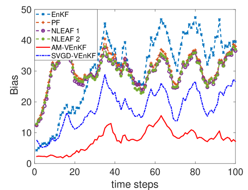
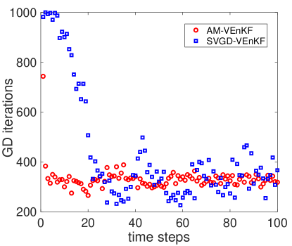
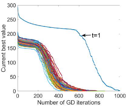
Figure 2: The average bias at each time step for $\theta=0$ and $M=100$ in the Lorenz 96 example.

Figure 3: Left: the number of GD iterations (in both AM and SVGD) at each time step. Right: the current best value plotted against the GD iterations (in AM) where each line represents a time step. The results are for $\theta=0$ and $M=100$ in the Lorenz 96 example.

The average bias for $\theta=0$ is shown in Fig. 3 where it can be observed that in this case, while the other three methods yield largely comparable accuracy in terms of estimation bias, the bias of AM-VEnKF is significantly smaller. To analyze the convergence property of the method, in Fig. 3 (left) we show the number of GD iterations (of both AM and SVGD) at each time step, where one can see that all GD iterations terminate after around 300-400 steps in AM-VEnKF, except the iteration at $t=1$ which proceeds for around 750 steps. The SVGD-VEnKF undergoes a much higher number of iterations in the first 20 time steps, while becoming about the same level as that of AM-VEnKF. This can be further understood by observing Fig. 3 (right) which shows the current best value $F^{*}_{k}$ with respect to the GD iteration in AM-VEnKF, and each curve in the figure represents the result at a time step $t$. We see here that the current best values become settled after around 400 iterations at all time locations except $t=1$, which agrees well with the number of iterations shown on the left. It is sensible that the GD algorithm takes substantially more iterations to converge at $t=1$, as the posterior at $t=1$ is typically much far away from the prior, compared to other time steps. These two figures thus show that the proposed stopping criteria are effective in this example.

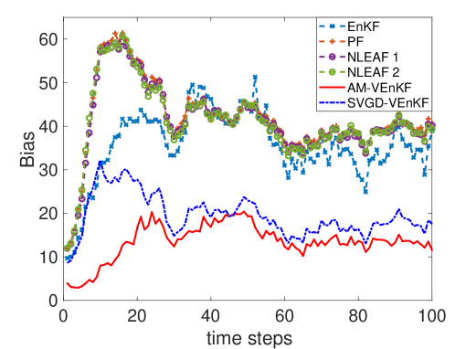
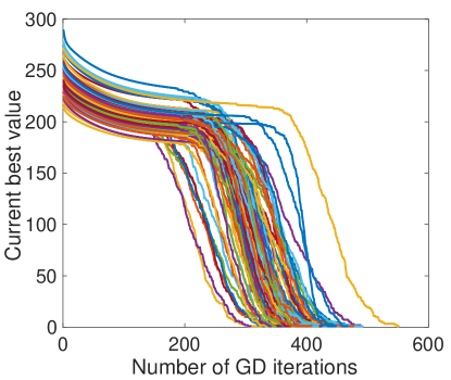
Figure 4: The average bias at each time step for $\theta=0.5$ and $M=100$ in the Lorenz 96 example.

Figure 5: Left: the number of GD iterations (in both AM and SVGD) at each time step. Right: the current best value plotted against the GD iterations (in AM) where each line represents a time step. The results are for $\theta=0.5$ and $M=100$ in the Lorenz 96 example.

The same sets of figures are also produced for $\theta=0.5$ (Fig. 5 for the average bias and Fig. 5 for the number of iterations and the current best values) and for $\theta=1$ (Fig. 7 for the average bias and Fig. 7 for the number of iterations and the current best values). Note that, in Fig. 7 the bias of EnKF is enormously higher than those of the other methods and so is omitted. The conclusions drawn from these figures are largely the same as those for $\theta=0$, where the key information is that VEnKF significantly outperforms the other methods in terms of estimation bias, and within VEnKF, the results of AM are better than those of SVGD. Regarding the number of GD iterations in AM-VEnKF, one can see that in these two cases (especially in $\theta=1$) it takes evidently more GD iterations for the algorithm to converge, which we believe is due to the fact that the noise in these two cases are not additive and so the observation models deviate further away from the Gaussian-linear setting.

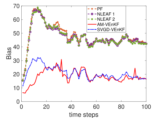
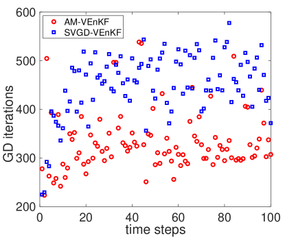
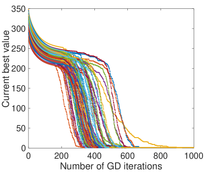
Figure 6: The average bias at each time step for $\theta=1$ and $M=100$ in the Lorenz 96 example.

Figure 7: Left: the number of GD iterations (in both AM and SVGD) at each time step. Right: the current best value plotted against the GD iterations (in AM) where each line represents a time step.The results are for $\theta=1$ and $M=100$ in the Lorenz 96 example.

As has been mentioned, we also conduct the experiments for a smaller sample size $M=20$ with localization employed, and we show the average bias results for $\theta=0$, $\theta=0.5$ and $\theta=1$ in Fig. 8. Similar to the larger sample size case, the bias is also averaged over 200 trials. In this case, we see that the advantage of VEnKF is not as large as that for $M=100$, but nevertheless VEnKF still yields clearly the lowest bias among all the tested methods. On the other hand, the results of the two VEnKF methods are quite similar while that of AM-VEnKF is slightly lower. Also shown in Fig. 8 are the number of GD iterations at each time step for all the three cases, which shows that the numbers of GD iterations used are smaller than their large sample size counterparts.

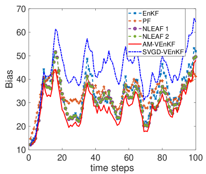
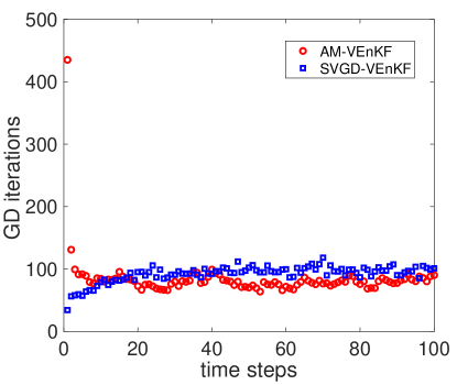
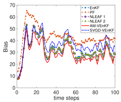
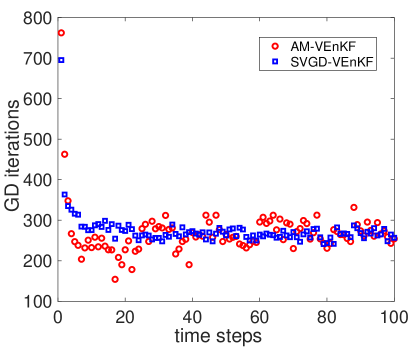
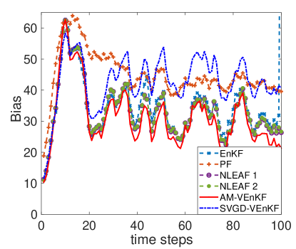
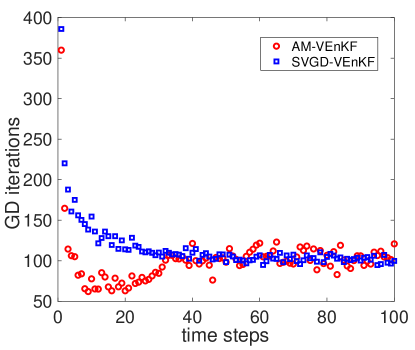
Figure 8: The results for $M=20$ in the Lorenz 96 example. The figures on the left show the average bias at each time step; the ones on the right show the number of GD iterations (in both AM and SVGD) at each time step. From top to bottom are respectively the results of $\theta=0$, 0.5 and 1.

4.3 Fisher’s equation

Our second example is the Fisher’s equation, a baseline model of wildfire spreading, where filtering is often needed to assimilate observed data at selected locations into the model [26]. Specifically, the Fisher’s equation is specified as follows,

$$c_{t}=Dc_{xx}+rc(1-c),\,\,0<x<L,\,\,t>0,$$ (27a)

$$c_{x}(0,t)=0,\,\,c_{x}(L,t)=0,\,\,c(x,0)=f(x),$$ (27b)

where $D=0.001$, $r=0.1$, $L=2$ are prescribed constants, and the noise-free initial condition $f(x)$ takes the form of,

$$f(x)=\left\{\begin{array}[]{rcl}0,&&0\leq x<L/4\\ {4x}/{L}-1,&&{L}/{4}\leq x<{L}/{2}\\ 3-{4x}/{L},&&{L}/{2}\leq x<{3L}/{4}\\ 0,&&{3L}/{4}\leq x\leq L.\end{array}\right.$$ (28)

In the numerical experiments we use an upwind finite difference scheme and discretize the equation onto $N_{x}=200$ spatial grid points over the domain $[0,\,L]$, yielding a 200 dimensional filtering problem. The time step size is determined by $D\frac{\Delta t}{\Delta x^{2}}=0.1$ with $\Delta x=\frac{L}{N_{x}-1}$ and the total number of time steps is 60. The prior distribution for the initial condition is $U[-5,5]+f(x)$, and in the numerical scheme a model noise is added in each time step and it is assumed to be in the form of $N(0,C)$, where

$$C(i,j)=0.3\exp(-(x_{i}-x_{j})^{2}/L),\ i,\ j=1,\ldots,N_{x},$$

with $x_{i},x_{j}$ being the grid points.

The observation is made at each grid point, and the observation model is as described in Section 4.1. Once again we test the three cases associated with $\theta=0,\,0.5$ and $1$. The ground truth and the data are both simulated from the model described above.

We test the same set of filtering methods as those in the first example. Since in practice, it is usually of more interest to consider a small ensemble size relative to the dimensionality, we choose to use 50 particles for this 200 dimensional example. Since the sample size is smaller than the dimensionality, the sliding window localization with $l=5$ and $k=3$ is used. All the simulations are repeated 200 times and the average biases are plotted in Fig. 9 for all the three cases ($\theta=0,\,0.5$ and $1$). We see that in all the three cases the two VEnKF methods result in the lowest estimation bias among all the methods tested, and the results of the two VEnKF methods are rather similar. It should be mentioned that, in the case of $\theta=1$, the bias of EnKF is omitted as it is enormously higher than those of the other methods.

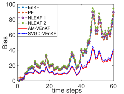
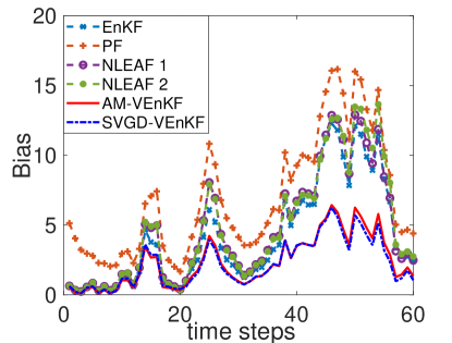
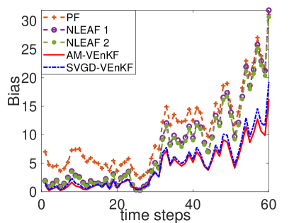
Figure 9: The average bias at each time step in the Fisher’s equation example. From top to bottom: $\theta=0$, $\theta=0.5$ and $\theta=1$.

As the bias results shown in Fig. 9 are averaged over all the dimensions, it is also useful to examine the bias at each dimension. We therefore plot in Fig. 10 the bias of each grid point at three selected time steps $t=10,\,30,$ and 60. The figures illustrate that, at all these time steps, the VEnKF methods yield substantially lower bias at the majority of the grid points, which is consistent with the average bias results shown in Fig. 9. We also report that, the wall-clock time for solving the optimization problem in each time step in AM-VEnKF is approximately 2.0 seconds (on a personal computer with a 3.6GHz processor and 16GB RAM), indicating a modest computational cost in this 200 dimensional example.

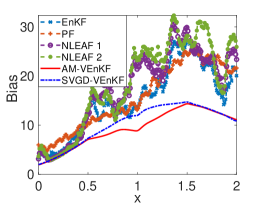
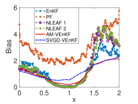
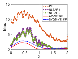
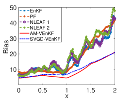
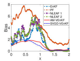
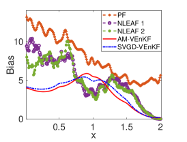
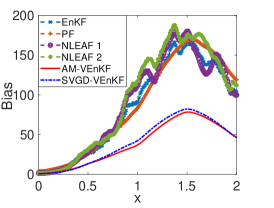
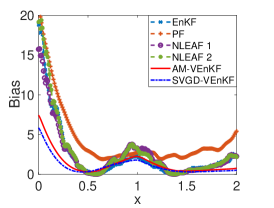
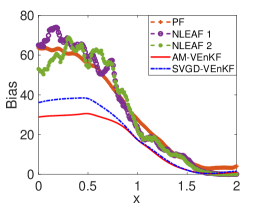
Figure 10: The estimation bias at $t=10$ (top), $t=30$ (middle) and $t=60$ (bottom), in the Fisher’s equation example. From left to right: $\theta=0$, $\theta=0.5$ and $\theta=1$.

4.4 Lorenz 2005 model

Here we consider the Lorenz 2005 model [24] which products spatially more smoothed model trajectory than Lorenz 96. The Lorenz 2005 model is written in the following scheme,

$$\frac{dx^{n}}{dt}=[x,x]^{K,n}-X^{n}+F,\quad n=1,\ldots,N.$$ (29)

where

$$[x,x]^{K,n}=\sum\limits_{j=-J}^{J}{{}^{\prime}}\sum\limits_{i=-J}^{J}{{}^{\prime}}(-x^{n-2K-i}x^{n-K-j}+x^{n-K+j-i}x^{n+K+j})/K^{2},$$

and this equation is composed with periodic boundary condition. $F$ is the forcing term and $K$ is the smoothing parameter while $K<<N$, and one usually sets $J=\frac{K-1}{2}$ if $K$ is odd, and $J=\frac{K}{2}$ if $K$ is even. Noted that the symbol $\sum{{}^{\prime}}$ denote a modified summation which is similarly with generally summation $\sum$ but the first and last term are divided by $2$. Moreover if $K$ is even the summation is $\sum{{}^{\prime}}$, and if $K$ is odd the summation is replaced by ordinary $\sum$.

It is worth noting that, when setting $K=1$, $N=40$, and $F=8$, the model reduces to Lorenz 96. In this example, we set the model as $N=560$, $F=10$ and $K=16$, resulting in a 560-dimensional filtering problem. Following the notations in Sec. 4.2, Lorenz 2005 is also represented by a standard discrete-time fourth-order Runge-Kutta solution of Eq. (29) with $\Delta t=0.01$ where the same model noise is added, and the state and observation pair $\{{\bf{x}}_{t},{\bf{y}}_{t}\}$ is similarly denoted by Eq. (26). We reinstate that in this example the observation model is chosen differently (see Sec. 4.1). And the initial state is chosen to be ${\bf{x}}_{0}\sim U[0,5]$.

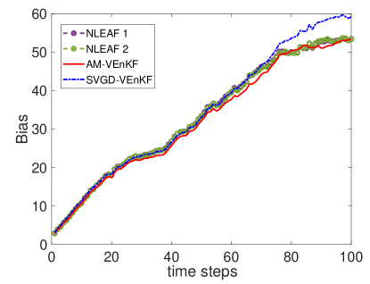
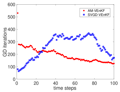
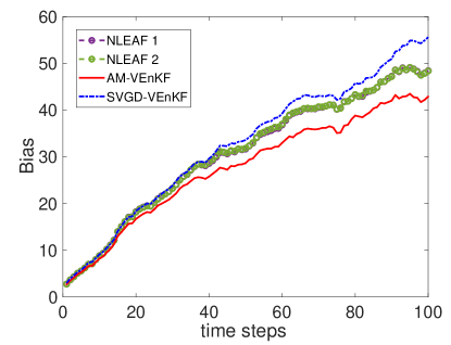
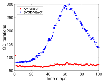
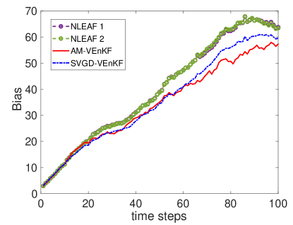
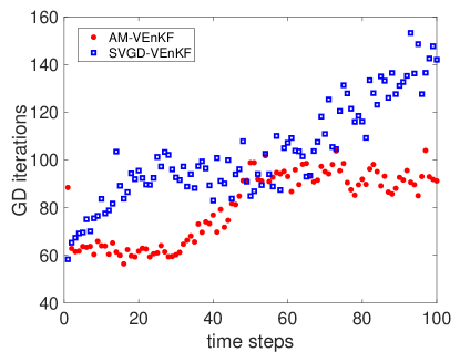
Figure 11: The results for the Lorenz 2005 example: the figures on the left show the average bias at each time step; the ones on the right show the number of GD iterations (in both AM and SVGD) at each time step. From top to bottom are respectively the results of $\theta=0$, 0.5 and 1.

In this numerical experiments, we test the same set of methods as those in the first two examples, where in each method 100 particles are used. Due to the small ensemble size, it is necessary to adopt the sliding-window localization with $(l,k)=(5,3)$ in all methods except PF. We observe that the errors in the results of EnKF and PF are significantly larger than those in the other methods, and so those results are not presented here. It should be noted that the stopping threshold is as $\Delta_{F}=0.5$ during nearest $\Delta_{k}=20$ iterations in AM-VEnKF. All methods are repeated 20 times and we plot the averaged bias and the averaged GD iterations for all the three cases ($\epsilon=0$, $0.5$ and $1$) in Fig. 11. One can see from the figures that, in the first case ($\epsilon=0$) the results of all the methods are quite similar, while in the other two cases, the results of AM-VEnKF are clearly better than those of all the other methods.

5 Closing Remarks

We conclude the paper with the following remarks on the proposed VEnKF framework. First we reinstate that, the Fisher’s equation example demonstrates that the KLD minimization problem in AM-VEnKF can be solved rather efficiently, and more importantly this optimization step does not involve simulating the underlying dynamical model. As a result, this step, though more complicated than the update in the standard EnKF, may not be the main contributor to the total computational burden, especially when the underlying dynamical model is computational intensive. Second, it is important to note that, although VEnKF can deal with generic observation models, it still requires that the posterior distributions are reasonably close to Gaussian, an assumption needed for all EnKF type of methods. For strongly non-Gaussian posteriors, it is of our interest to explore the possibility of incorporating VEnKF with some existing extensions of EnKF that can handle strong non-Gaussianity, such as the mixture Kalman filter [33]. Finally, in this work we provide two transform mappings, the affine mapping and the RKHS mapping in the SVGD framework. In the numerical examples studied here, the affine mapping seems to achieve a better performance, but we acknowledge that more comprehensive comparisons should be done to understand the advantages and limitations of different types of mappings. A related issue is that, some existing works such as [29] use more flexible and complicated mappings and so that they can approximate arbitrary posterior distributions. It is worth noting, however, this type of methods are generally designed for problems where a rather large number of particles can be afforded, and therefore are not suitable for the problems considered here. Nevertheless, developing more flexible mapping based filters is an important topic that we plan to investigate in future studies.

Appendix A SVGD-VEnKF

In this section, we discuss the procedure for constructing the mapping using the Stein variational gradient descent (SVGD) formulation [22], which provides a nonlinear transform from the prior to the posterior in each time step.

Recall that in Section 3 we want to find a mapping by solving

$$\min_{T\in\mathcal{H}}{\mathcal{D}}_{\mathrm{KL}}(\pi_{T},q),$$ (30)

where $q(\cdot)=\hat{\pi}(\cdot|y_{1:t})$ and $\mathcal{H}$ is a certain function space that will be specified later.

Following the same argument in Sec. 3.3, we obtain that Eq. (30) is equivalent to,

$$\min_{T\in\mathcal{H}}{\mathcal{D}}_{\mathrm{KL}}(p(\tilde{x}),q_{T^{-1}}(\tilde{x})),$$ (31)

where $q_{T^{-1}}(\cdot)$ is as defined in Section 3.3.

Now we need to determine the function space $\mathcal{H}$. While in the proposed AM-VEnKF method $\mathcal{H}$ is chosen to be an affine mapping space, the SVGD framework specifies $\mathcal{H}$ via a reproducing kernel Hilbert space (RKHS) [31].

First we write the mapping $T$ in the form of,

$$T(\tilde{x})=\tilde{x}+\tau\phi(\tilde{x}),$$ (32)

where $\tau$ is a prescribed stepsize. Next we assume that mapping $\phi$ is chosen from a RKHS $\mathcal{H}_{K}$ specified by a reproducing kernel $K(\cdot,\cdot)$. Therefore the optimisation problem (31) becomes,

$$\min_{\phi\in\mathcal{H}_{K}}{\mathcal{D}}_{\mathrm{KL}}(p(\tilde{x}),q_{T^{-1}}(\tilde{x})).$$ (33)

In the SVGD framework, one does not seek to solve the optimisation problem in Eq. (33) directly; instead it can be derived that the direction of steepest descent is

$$\phi^{*}(\cdot)=\mathrm{E}_{\tilde{x}\sim p}[\nabla_{\tilde{x}}\log q(\tilde{x})K(\tilde{x},\cdot)+\nabla_{\tilde{x}}K(\tilde{x},\cdot)].$$ (34)

It should be noted that we omit the detailed derivation of Eq. (34) here and interested readers may consult [22] for such details. The obtained mapping $\phi^{*}$ is then applied to the samples which pushes them toward the target distribution. This procedure is repeated until certain stopping conditions are satisfied. The complete SVGD based VEnKF algorithm is given in Alg. 2. Finally we note that, in the numerical experiments we use the squared exponential kernel with bandwidth $h$:

$$K(x,x^{\prime})=\exp(-\|x-x^{\prime}\|_{2}^{2}/h),$$

where the implementation details can be found in [22].

Algorithm 2 SVGD based variational EnKF (SVGD-VEnKF)

• Prediction:

  • Let $\tilde{x}_{t}^{m}=F_{t}(x_{t-1}^{m},\alpha_{t}^{m}),m=1,2,\ldots,M$;

  • Let $\hat{\pi}(\cdot|y_{1:t-1})=N(\tilde{\mu}_{t},\tilde{\Sigma}_{t})$ where $\tilde{\mu}_{t}$ and $\hat{\Sigma}_{t}$ are computed using Eq. (9);

• Update:

  • Let $q(\cdot)=\hat{\pi}(\cdot|y_{1:t})\propto\hat{\pi}(\cdot|y_{1:t-1})\pi(y_{t}|\cdot)$;

  • Repeat the following steps until the stopping conditions are satisfied;

    • Let

      $$\tilde{\phi}^{*}(\cdot)=\frac{1}{M}\sum\limits_{m=1}^{M}[\nabla_{\tilde{x}_{t}^{m}}\log q(\tilde{x}_{t}^{m})K(\tilde{x}_{t}^{m},\cdot)+\nabla_{\tilde{x}_{t}^{m}}K(\tilde{x}_{t}^{m},\cdot)].$$

    • Let $\tilde{x}_{t}^{m}\leftarrow\tilde{x}_{t}^{m}+\tau\tilde{\phi}^{*}({\tilde{x}_{t}^{m}}$), $m=1,\ldots,M$.

  • Let $x_{t}^{m}=\tilde{x}_{t}^{m}$, for $m=1,\ldots,M$.

References

- [1] Jeffrey L Anderson. An ensemble adjustment kalman filter for data assimilation. Monthly weather review, 129(12):2884–2903, 2001.
- [2] Jeffrey L Anderson. A local least squares framework for ensemble filtering. Monthly Weather Review, 131(4):634–642, 2003.
- [3] Jeffrey L Anderson. Exploring the need for localization in ensemble data assimilation using a hierarchical ensemble filter. Physica D: Nonlinear Phenomena, 230(1-2):99–111, 2007.
- [4] M S Arulampalam, Simon Maskell, Neil J Gordon, and T Clapp. A tutorial on particle filters for online nonlinear/non-gaussian bayesian tracking. IEEE Transactions on Signal Processing, 50(2):174–188, 2002.
- [5] H Auvinen, Johnathan M Bardsley, Heikki Haario, and T Kauranne. The variational kalman filter and an efficient implementation using limited memory bfgs. International Journal for Numerical Methods in Fluids, 64(3):314–335, 2010.
- [6] Yuming Ba, Lijian Jiang, and Na Ou. A two-stage ensemble kalman filter based on multiscale model reduction for inverse problems in time fractional diffusion-wave equations. Journal of Computational Physics, 374:300–330, 2018.
- [7] Peter Bauer, Alan Thorpe, and Gilbert Brunet. The quiet revolution of numerical weather prediction. Nature, 525(7567):47–55, 2015.
- [8] Matthew J Beal, Zoubin Ghahramani, and Carl Edward Rasmussen. The infinite hidden markov model. Advances in neural information processing systems, 1:577–584, 2002.
- [9] Alex Capaldi, Samuel Behrend, Benjamin Berman, Jason Smith, Justin Wright, and Alun L Lloyd. Parameter estimation and uncertainty quantication for an epidemic model. Mathematical biosciences and engineering, page 553, 2012.
- [10] Zhe Chen et al. Bayesian filtering: From kalman filters to particle filters, and beyond. Statistics, 182(1):1–69, 2003.
- [11] Arnaud Doucet and Adam M Johansen. A tutorial on particle filtering and smoothing: Fifteen years later. Handbook of nonlinear filtering, 12(656-704):3, 2009.
- [12] Tarek A El Moselhy and Youssef M Marzouk. Bayesian inference with optimal maps. Journal of Computational Physics, 231(23):7815–7850, 2012.
- [13] Geir Evensen. The ensemble kalman filter: Theoretical formulation and practical implementation. Ocean dynamics, 53(4):343–367, 2003.
- [14] Geir Evensen. Data assimilation: the ensemble Kalman filter. Springer Science & Business Media, 2009.
- [15] Shai Fine, Yoram Singer, and Naftali Tishby. The hierarchical hidden markov model: Analysis and applications. Machine learning, 32(1):41–62, 1998.
- [16] Marco Frei and Hans R Künsch. Bridging the ensemble kalman and particle filters. Biometrika, 100(4):781–800, 2013.
- [17] Peter L Houtekamer and Herschel L Mitchell. Data assimilation using an ensemble kalman filter technique. Monthly Weather Review, 126(3):796–811, 1998.
- [18] Peter L Houtekamer and Herschel L Mitchell. A sequential ensemble kalman filter for atmospheric data assimilation. Monthly Weather Review, 129(1):123–137, 2001.
- [19] Anders Krogh, Björn Larsson, Gunnar Von Heijne, and Erik LL Sonnhammer. Predicting transmembrane protein topology with a hidden markov model: application to complete genomes. Journal of molecular biology, 305(3):567–580, 2001.
- [20] Jing Lei and Peter Bickel. A moment matching ensemble filter for nonlinear non-gaussian data assimilation. Monthly Weather Review, 139(12):3964–3973, 2011.
- [21] Weixuan Li, W Steven Rosenthal, and Guang Lin. Trimmed ensemble kalman filter for nonlinear and non-gaussian data assimilation problems. arXiv preprint arXiv:1808.05465, 2018.
- [22] Qiang Liu and Dilin Wang. Stein variational gradient descent: a general purpose bayesian inference algorithm. In Proceedings of the 30th International Conference on Neural Information Processing Systems, pages 2378–2386, 2016.
- [23] Edward N Lorenz. Predictability: A problem partly solved. In Proc. Seminar on predictability, volume 1, 1996.
- [24] Edward N Lorenz. Designing chaotic models. Journal of Atmospheric Sciences, 62(5):1574–1587, 2005.
- [25] David JC MacKay. Information theory, inference and learning algorithms. Cambridge university press, 2003.
- [26] Jan Mandel, Lynn S Bennethum, Jonathan D Beezley, Janice L Coen, Craig C Douglas, Minjeong Kim, and Anthony Vodacek. A wildland fire model with data assimilation. Mathematics and Computers in Simulation, 79(3):584–606, 2008.
- [27] Edward Ott, Brian R Hunt, Istvan Szunyogh, Aleksey V Zimin, Eric J Kostelich, Matteo Corazza, Eugenia Kalnay, DJ Patil, and James A Yorke. A local ensemble kalman filter for atmospheric data assimilation. Tellus A: Dynamic Meteorology and Oceanography, 56(5):415–428, 2004.
- [28] Edward Posner. Random coding strategies for minimum entropy. IEEE Transactions on Information Theory, 21(4):388–391, 1975.
- [29] Manuel Pulido and Peter Jan van Leeuwen. Sequential monte carlo with kernel embedded mappings: The mapping particle filter. Journal of Computational Physics, 396:400–415, 2019.
- [30] M. Roth, E. Özkan, and F. Gustafsson. A student’s t filter for heavy tailed process and measurement noise. In 2013 IEEE International Conference on Acoustics, Speech and Signal Processing, pages 5770–5774, 2013.
- [31] Bernhard Scholkopf and Alexander J Smola. Learning with kernels: support vector machines, regularization, optimization, and beyond. Adaptive Computation and Machine Learning series, 2018.
- [32] Antti Solonen, Heikki Haario, Janne Hakkarainen, Harri Auvinen, Idrissa Amour, and Tuomo Kauranne. Variational ensemble kalman filtering using limited memory bfgs. Electronic Transactions on Numerical Analysis, 39:271–285, 2012.
- [33] Andreas S Stordal, Hans A Karlsen, Geir Nævdal, Hans J Skaug, and Brice Vallès. Bridging the ensemble kalman filter and particle filters: the adaptive gaussian mixture filter. Computational Geosciences, 15(2):293–305, 2011.
- [34] Jeffrey S Whitaker and Thomas M Hamill. Ensemble data assimilation without perturbed observations. Monthly weather review, 130(7):1913–1924, 2002.