AI Powered Compiler Techniques for DL Code Optimization

Abstract.

Creating high performance implementations of deep learning primitives on CPUs is a challenging task. Multiple considerations including multi-level cache hierarchy, and wide SIMD units of CPU platforms influence the choice of program transformations to apply for performance optimization. In this paper, we present machine learning powered compiler techniques to optimize loop nests. We take a two-pronged approach to code optimization: We first apply high level optimizations to optimize the code to take optimal advantage of the cache memories. Then, we perform low level, target-specific optimizations to effectively vectorize the code to run well on the SIMD units of the machine. For high level optimizations, we use polyhedral compilation techniques and deep learning approaches. For low level optimization, we use a target specific code generator that generates code using vector intrinsics and Reinforcement Learning (RL) techniques to find the optimal parameters for the code generator. We perform experimental evaluation of the developed techniques on various matrix multiplications that occur in popular deep learning workloads. The experimental results show that the compiler techniques presented in the paper achieve 7.6X and 8.2X speed-ups over a baseline for sequential and parallel runs respectively.

1. Introduction

Deep learning (DL) has become pervasive in various domains of computing. Image recognition (Krizhevsky et al., 2012; He et al., 2016), language modeling (Devlin et al., 2018), language translation (Wu et al., 2016), speech recognition (Hinton et al., 2012) make extensive use of deep neural networks (DNNs). Deep Learning inference is an important workload across applications, such as object classification & recognition, text and speech translation etc. A 2018 Mc Kinsey study (Batra et al., 2018) pointed out that in datacenters, 75% of the inference tasks are run on CPUs. Optimizing DL workloads on CPUs is a challenging proposition because of architectural complexities of CPU platforms. Multi-level cache hierarchies, TLBs (Translation Look-aside Buffers), hardware data prefetchers, SIMD (a.k.a vector) units present particular challenges in writing high performance code. Therefore, the current state-of-practice is to use expert-coded high performance libraries such as Intel oneDNN (int, 2020) in deep learning frameworks such as TensorFlow and PyTorch to achieve good performance. However, being reliant on libraries for performance is not scalable. First, it would increase the time-to-market: from the time a new DL operator is invented to its being supported in a library could take a considerable amount of time. Second, even expert programmers must invest significant amount of effort to tune the implementations on the target platforms. Therefore, an attractive alternative solution is to develop compilation techniques that automate code optimization and achieve similar performance levels as expert-coded libraries.

In this paper, we develop a systematic approach to automatic code optimization. We categorize the program optimizations into two phases: high level and low level optimizations. High level optimizations perform loop optimizations such as loop reordering and tiling to derive a loop structure that utilizes the cache hierarchy of the computer system to the fullest extent possible. Low level optimizations generate vector code using the target machine’s intrinsics; reinforcement learning methodology guides the derivation of high performance vector code. For high-level and low-level optimizations we leverage artificial intelligence (A.I.) techniques. We evaluate our automated compiler system on GEMMs which lie at the heart of deep learning (gem, 2015). The results indicate our compiler workflow delivers competitive performance compared to Intel oneDNN library and significantly higher performance compared to a state-of-the-art DL compiler, viz., AutoTVM (Chen et al., 2018b).

The contributions of the paper are as follows.

• A systematic approach to program optimization with clear demarcation of high-level and low-level optimizations that map well to the hardware architectures.

• Low-level optimizations that generate reinforcement learning (RL) guided vector intrinsics based code.

• Development of A.I. techniques for high-level and low-level optimizations.

• Experimental evaluation on various GEMM sizes that occur in DL workloads.

The rest of the paper is organized as follows. Section 2 introduces the overall compilation workflow. Section 3 describes the polyhedral compilation techniques we use for high level optimizations. The low-level optimizations involving the target platform specific code generator and reinforcement learning are developed in Section 4. The experimental evaluation conducted is detailed in Section 5. Related work is discussed in Section 6. The conclusion and implication of the presented work are presented in Section 7.

Figure 1. The compiler optimizations workflow

2. The Compiler Optimization Workflow

We first describe the overall compiler workflow. We input the loop nests such as GEMMs to the compiler. The high level optimizer first optimizes the loop structure and then passes on the code to the low level optimer. Figure 1 shows the workflow of the optimization process.

The high level optimizer uses polyhedral compilation techniques for optimization of the loop structure to take advantage of the multi-level caches of the CPU platform. The loop reordering and tiling transformations are applied and the best loop order and tile sizes are determined by the high level optimizer. It will enhance data locality – both the spatial and temporal locality such that the data used by the input program is reused out of the caches closest to the processor as much as possible. Section 3 details the polyhedral compilation techniques we apply for loop optimization.

The high level optimer then hands over the optimized code to the low-level optimizer. The low level optimizer derives a vectorization strategy for effective use of the SIMD vector units. We employ a target specific low level optimization approach wherein the inner loops of the loop nest are vectorized using the target-specific vector intrinsics. Further, we use a Reinforcement Learning (RL) based approach to select the best vectorization plan among the myriad choices available.

Jouppi et al (Jouppi et al., 2017) show that 95% of the deep learning inference workloads (MLPs, CNNs, and LSTMs) can be formulated in terms of matrix-multiplication. Matrix multiplication is at the heart of deep learning (gem, 2015). Because of these reasons in this work, we build the low level optimizer to optimize the matrix-multiplications that occur in the inner most loops of convolutions and matrix-multiplications themselves (matrix-multiplication can be recursively defined where the other loops of the code are the tiled loops and the inner loops are also functionally equivalent to matrix-multiplication). In Section 4, we describe the design and the implementation of the low level optimizer for the inner loops of the loop nest focused on matrix multiplication.

3. High-level Polyhedral Loop Optimizations

We use the polyhedral model (Feautrier, 1996), which is an advanced mathematical framework to reason about dependences and loop transformations, to develop our data reuse algorithm.

3.1. Preliminaries

We use the Integer Set Library (ISL) (Verdoolaege, 2010) for performing polyhedral operations in this work and we use the same notation as used in ISL to elucidate the concepts and the algorithm. The matrix multiplication code shown in Figure 2 will be used to illustrate the workings of the data reuse analysis.

⬇

for (i = 0; i < M; i++) {

for (j = 0; j < N; j++) {

for (k = 0; k < K; k++) {

C[i][j] += A[i][k] * B[k][j];

}

}

}

Figure 2. Matrix multiplication code

Sets

A set is a tuple of variables $x_{i}$s along with a collection of constraints $c_{k}$s defined on the tuple variables. $s=\{[x_{1},\dots,x_{n}]:c_{1}\land\dots c_{m}\}$

The iteration spaces of loop nests are represented as sets. The iteration space of the loop in Figure 2 is defined as the following set. $I=\{S[i,j,k]:0<=i<M\land 0<=j<N\land 0<=k<K\}$

Relations

A relation is a mapping from input tuple variables $x_{i}$s to output tuple variables $y_{j}$s. In addition, a set of constraints $c_{k}$s can be defined for a relation that will place constraints on the input/output tuple variables. $r=\{[x_{1},\dots,x_{n}]\mapsto[y_{1},\dots,y_{m}]:c_{1},\dots,c_{p}\}$

The read and write access functions of a loop nest can be modeled with relations. The read relations in the Figure 2 code are shown below: $r_{1}=\{S[i,j,k]\mapsto C[i,j]\}$, $r_{2}=\{S[i,j,k]\mapsto A[i,k]\}$, $r_{3}=\{S[i,j,k]\mapsto B[k,j]\}$. The sole write relation in the loop is: $w_{1}=S[i,j,k]\mapsto C[i,j]$. The domain of a relation $r$ is denoted by dom $r$.

Apply operation

When a relation $r$ is applied on a set $s$, the domain of $r$ will be intersected with $s$ and the resulting range will be a new set $s^{\prime}$. The set $s^{\prime}$ is said to be the result of the apply operation. The operation is mathematically defined as: $(\vec{y}\in s^{\prime})\Longleftrightarrow(\exists\vec{x}~{}~{}\text{s.t}~{}~{}(\vec{x}\in s\land\vec{x}\mapsto\vec{y})\in r)$

The data footprint of the loop can be computed by applying read and write relations on the iteration space set: $r_{1}(I)\cup r_{2}(I)\cup r_{3}(I)\cup w_{1}(I)$

Lexicographic operations

The lexicographical operations can be applied on sets. $s_{1}<<s_{2}$ outputs all the elements of $s_{1}$ that are lexicographically strictly smaller than all the elements of $s_{2}$, while $s_{1}<<=s_{2}$ gets us the elements of $s_{1}$ that are lexicographically smaller than or equal to the elements of $s_{2}$. The lexicographically smallest element of a set $s$ is queried using lexmin $s$. Similarly, the lexicographically largest element is obtained using lexmax $s$.

Set difference.

The set difference between set $s_{1}$ and $s_{2}$ is denoted by $s_{1}-s_{2}$, i.e., the resulting set will have elements of $s_{1}$ that do not appear in $s_{2}$.

Polyhedral dependences.

The exact data dependences in loop nests can be computed in the polyhedral model and are expressed as maps from source iterations to target iterations involved in the dependence. For cache data reuse analysis developed in §3.2, we consider four kinds of dependences – Read-After-Read (RAR), Read-After-Write (RAW, a.k.a flow), Write-After-Read (WAR, a.k.a anti), and Write-After-Write (WAW). The data dependencies of the matrix multiplication code in Figure 2 are shown below.

$$d_{1}= \{S[i,j,k]\mapsto S[i^{\prime},j^{\prime},k^{\prime}]:i^{\prime}=i\land j^{\prime}=j\land k<k^{\prime}<K\}$$

$$d_{2}= \{S[i,j,k]\mapsto S[i^{\prime},j^{\prime},k^{\prime}]:i^{\prime}=i\land k^{\prime}=k\land j<j^{\prime}<N\}$$

$$d_{3}= \{S[i,j,k]\mapsto S[i^{\prime},j^{\prime},k^{\prime}]:j^{\prime}=j\land k^{\prime}=k\land i<i^{\prime}<M\}$$

The dependence $d_{2}$ is induced by array reference A[i][k]. An element of array A, say A[0][0] which is accessed in source iteration $[i=0,j=0,k=0]$ gets reused in target iterations $[i^{\prime}=0,j^{\prime}>0,k^{\prime}=0]$. The source to target iteration relationships such as this are expressed in a parametric fashion as the relation $d_{2}$.

3.2. Loop transformations

We create a number of code variants by applying loop reordering and tiling transformations and using the PolyDL techniques (Tavarageri et al., 2021) select the top code variants.

Working set size computation

We perform cache data reuse analysis to characterize a loop-nest’s behavior with respect to a given cache hierarchy. The analysis computes the various existing data reuses of a program and then for the input cache hierarchy determines which data reuses are exploitable at various levels of cache. Each data dependence in a loop is also an instance of data reuse – the source and target iterations involved in the dependence touch the same data element and therefore, the data is reused. For a data dependence and hence data reuse to be realizable in a given level of cache, all the data elements accessed between the source and target iterations of the dependence – the working set – have to be retained in the cache so that when the execution reaches the target iteration, the data element(s) used in the source iteration will still be present in the cache.

We illustrate the computation of the working set sizes using the running example in Figure 2. Let us examine the following dependence carried by the $j$ loop arising because of the array reference $A[i][k]$: $d_{2}=\{S[i,j,k]\mapsto S[i^{\prime},j^{\prime},k^{\prime}]:i^{\prime}=i\land k^{\prime}=k\land j<j^{\prime}<N\}$. Of all the source iterations, the first/lexicographically minimum iteration is: $\mathcal{I}_{source}=\{S[i=0,j=0,k=0]\}$ Its target iterations are: $\{S[i=0,j,k=0]:0<j<N\}$. Among the target iterations, the first one is: $I_{min\_tar}=\{S[i=0,j=1,k=0]\}$ and the last one is: $I_{max\_tar}=\{S_{3}[i=0,j=N-1,k=0]\}$

The number of data elements of the three arrays – A, B, C accessed between $\mathcal{I}_{source}$ and $I_{min\_tar}$ is derived by applying the read and write relations on the intervening iteration set and it is:

$$WS_{min}=2K+3$$

The $K$ elements of array A – $A[0][0,1,\dots,K-1]$, the $K+1$ elements of array B – $B[0,1,\dots,K-1][0]$ and $B[0][1]$, and finally $2$ elements of array C – $C[0][0],C[0][1]$ accessed between the source iteration $S[i=0,j=0,k=0]$ and the target iteration $I_{min\_tar}=S[i=0,j=1,k=0]$ lead to the $WS_{min}$ size of $2K+3$.

The maximum working set size – the number of data elements touched between $\mathcal{I}_{source}$ and $I_{max\_tar}$ is:

$$WS_{max}=N\times K+N+1$$

The $WS_{max}$ size is arrived at by counting the number of array elements accessed between the source iteration - $S[i=0,j=0,k=0]$ and the target iteration - $I_{max\_tar}=\{S_{3}[i=0,j=N-1,k=0]\}$. As far as array A is concerned, $K$ elements of it – $A[0][0,1,\dots,K-1]$ are read. Array B’s elements – $B[0,1,\dots,K-1][0,1,\dots,N-2]$ plus $B[0][N-1]$ are read which total $K\times(N-1)+1$. $N$ elements of array C are read and written – $C[0][0,1,\dots,N-1]$. Therefore, a total of $N\times K+N+1$ are read and written.

We have built a code generator to emit a number of program variants. The code generator creates the loop variants by applying tiling and loop interchange program transformations. The tile sizes are varied as well. The working set size computation analysis is performed on each program version generated. Among the many variants generated, the ranking algorithm described below picks the top $k$ best performing versions, where $k$ is a parameter.

DNN-based code ranking algorithm.

We assume fully associative, and exclusive caches. If the working set size corresponding to a data reuse in the program is smaller than the cache size then the data reuse is exploitable in the cache. The ranking system considers caches at different levels (typically L1, L2, and L3) and for each data reuse, determines at what level of cache hierarchy is the data reuse realizable. We now describe the algorithm to determine the cumulative working set sizes at each level of cache. The inputs to the algorithm are the working set sizes computed for a loop nest, and the cache sizes of the target system. The algorithm determines the fastest level of cache where the working set size corresponding to each data reuse fits and adds it to that cache’s working set size. If a working set does not fit in any cache, then the data reuse happens out of the main memory. Consequently, the memory’s working set size is updated.

We use a deep neural network (DNNs) for ranking of code variants. For the purposes of training the DNN model, we collect the performance data of code variants generated and compute their working set sizes at different levels of the memory hierarchy. We train the DNN model to perform relative ordering of two code variants. We then use a tournament based ranking system to assign ranks to the different code versions created – we play each code variant against every other code variant. For each variant, we record the number of wins it has accumulated. We then rank the variants based on the number of wins – the higher the number of wins, the higher the rank.

Figure 3. The DNN architecture for ranking of code variants. The DNN shown is a representative figure.

We use a four layer feed forward neural network architecture shown in Figure 3. We normalize the compiler generated working set sizes using min-max scaling: $\frac{x-x_{min}}{x_{max}-x_{min}}$. Each value is subtracted with the minimum value in that feature column and divided by the feature range. The output layer consists of two neurons and we use the softmax function for the output layer. The values of the two output neurons, because of the use of the softmax function, sum to 1. If the output value is above a threshold - $\theta$, we consider it a 1, otherwise a 0. If the first neuron fires a 1, then the first variant is considered the winner. If the second neuron fires a 1, then the second variant is considered the winner. If both of them are zero because none of them are above the threshold, then it is a draw between the two variants. In this work, we set the threshold $\theta$ to 0.7. We experimented with deeper models as well. However, depth beyond four did not have any discernible effect on accuracy.

4. Low-level Target Specific Inner Loop Optimizations

The high level optimizations as described in §3 are first applied to the input code and then the inner loops are handed over the low level optimizer. The low level optimizer focuses on vectorization and assumes that the data used by the inner loops is resident in L1 cache. The inner loops are analyzed to find out which loops are parallel and hence, vectorizable. The different vectorizable loops present us multiple choices for vectorization. Further, unroll-and-jam (the loops are unrolled and the unrolled statements are combined in the inner-most loop) can present various data reuse opportunities. Thus, the various unroll factors for the loops give rise to multiple ways of vectorizing the loops and we have to select a scheme that leads to the highest performance. To help select the best vectorization parameters, namely, the unroll factors for the loops, we use Reinforcement Learning (RL).

⬇

for (i = 0; i < M; i++) {

for (j = 0; j < N; j+=16) {

for (k = 0; k < K; k++) {

C[i][j] += A[i][k] * B[k][j];

C[i][j+1] += A[i][k] * B[k][j+1];

C[i][j+2] += A[i][k] * B[k][j+2];

…

C[i][j+15] += A[i][k] * B[k][j+15];

}

}

}

Figure 4. Unrolled GEMM code for unroll factors 1, 16, 1

⬇

M_full = (M / 1) * 1 ;

N_full = (N / 16) * 16 ;

K_full = (K / 1) * 1 ;

for (i = 0; i < M_full; i += 1) {

for (j = 0; j < N_full; j += 16) {

vecC = _mm512_load_ps(&C[i*CStride+j]);

for (k = 0; k < K_full; k += 1) {

vecA =_mm512_set1_ps(A[i*AStride + k]);

vecB =_mm512_load_ps(&B[k*BStride+j]);

vecC =_mm512_fmadd_ps(vecA,vecB,vecC);

}

_mm512_store_ps(&C[i*CStride + j], vecC);

}

}

// The residue code for non-full M, N, K

// values omitted for brevity.

Figure 5. Auto-generated GEMM code using AVX-512 intrinsics for unroll factors 1, 16, 1

⬇

M_full=(M / 2) * 2 ;

N_full=(N / 16) * 16 ;

K_full=(K / 2) * 2 ;

for (i=0; i < M_full; i+=2) {

for (j=0; j < N_full; j+=16) {

vecC=_mm512_load_ps(&C[i*CStride+j]);

vecC1=_mm512_load_ps(&C[(i+1)*CStride+j]);

for (k=0; k < K_full; k+=2) {

vecA=_mm512_set1_ps(A[i*AStride+k]);

vecB=_mm512_load_ps(&B[k*BStride+j]);

vecB1=_mm512_load_ps(&B[(k+1)*BStride+j]);

vecA1=_mm512_set1_ps(A[i*AStride+(k+1)]);

vecA2=_mm512_set1_ps(A[(i+1)*AStride+k]);

vecA3=_mm512_set1_ps(A[(i+1)*AStride+(k+1)]);

vecC=_mm512_fmadd_ps(vecA,vecB,vecC);

vecC1=_mm512_fmadd_ps(vecA2,vecB,vecC1);

vecC=_mm512_fmadd_ps(vecA1,vecB1,vecC);

vecC1=_mm512_fmadd_ps(vecA3,vecB1,vecC1);

}

_mm512_store_ps(&C[i*CStride+j], vecC);

_mm512_store_ps(&C[(i+1)*CStride+j], vecC1);

}

}

// The residue code for non-full M, N, K

// values omitted for brevity.

Figure 6. Auto-generated GEMM code using AVX-512 intrinsics for unroll factors 2, 16, 2

4.1. Vector intrinsic based code generation

We illustrate the workings of the vectorization scheme and the use of RL on GEMM inner loops. Figure 4 shows the matrix multiplication code where the j loop is unrolled by a factor of 16 and the statements are moved to the inner most loop (unroll-and-jam). Because the j loop is parallel, it is vectorizable. We have built a code generator that generates the vectorized code using the vector intrinsics of the target CPU platform. Figure 5 shows the generated code using AVX-512 intrinsics to run on vector units that can work on 512 bits of data simultaneously. The datatype of the variables in the shown code is 32 bit floating point numbers. Therefore, we can perform arithmetic operations on 16 floating point numbers ($16\times 32=512$) at the same time. In Figure 4, we observe that the same array element – “A[i][k]” is used in all 16 arithmetic operations. Therefore, it is broadcast to all elements of the vector register using the _mm512_set1_ps vector intrinsic. The 16 elements of the C array – “C[i][j]” through “C[i][j+15]” are loaded using the _mm512_load_ps vector intrinsic. Since the loaded C elements are reused in all of the inner-most k loop, the loading is hoisted out of the k loop. In a similar fashion, the 16 elements of the B array – “B[k][j]” through “B[k][j+15]” are loaded using the _mm512_load_ps vector intrinsic. The 16 addition and multiplication operations are performed using the fused-multiply-add operation through the intrinsic _mm512_fmadd_ps. After the C vector is accumulated into in the k loop, the results are stored back into the C array using _mm512_store_ps outside of the k loop.

In the GEMM code, all three loops – i,j, and k loops carry data reuse. Consequently, when we unroll any of the loops, that leads to reuse of the data of one of the three arrays – A, B, and C. For example, in Figure 6, the i loops is unrolled by a factor of 2 and it leads to reuse of the array B: The array access expression for B is “B[k][j]” and it is free of the i loop variable and therefore for all values of i, the same B array element would be used. In the code we observe that vecB is used in two fused-multiply-add operations – while computing vecC and vecC1. When we unroll the inner-most k loop, that helps us schedule the load and fma operations further apart thereby increasing the chances of the data being loaded in the vector registers when the execution reaches the fma operations.

Thus, by unrolling various loops we can increase the data reuse in vector registers, and schedule the load operations in such a way that memory latency is tolerated well. However, because the number of vector registers is limited, a certain choice of an unroll factor for a loop will impose constraints on the unroll factors of other loops. The interplay between the amount of data reuse, scheduling, and the impact of data reuse of different arrays could be complex. We use reinforcement learning which in turn uses a neural network to determine the best unroll factors for the loops.

4.2. Reinforcement Learning

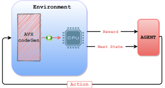
Figure 7. Reinforcement Learning for target specific low level optimization.

The choices of unroll factors for the inner loops constitute the state space for reinforcement learning (RL). The agent will suggest whether to increase unroll factors or to decrease them. The increment/decrement of the unroll factors form the actions. The target specific code generator will carry out the actions suggested by the agent by generating code with the new unroll factors and the code is run on the target platform. The actions will either lead to a higher performance or a lower performance vis-a-vis the performance of the prior state. If the action leads to a higher performance, we will encode it as a positive reward – the relative performance increase. If the action causes the performance to degrade, it is denoted as a negative reward – the relative performance decrease. Figure 7 shows the RL set-up.

The agent will use a neural network to suggest next actions to undertake. While the state space exploration is being conducted, we will have two phases – exploration, and exploitation. In the exploration phase, the agent will recommend random actions and the reward obtained will be used to continually train the neural network to predict actions that will lead to larger positive rewards and thus higher performance states. In the exploitation phase, the agent will query the neural network for the best actions – actions that will lead to the biggest rewards. The transitions between the exploration and exploitation phases are controlled by the exploration decay rate. We set it in such a way that at initial stages exploration is selected more often, and later exploitation is chosen more.

We train a neural network to encode the policy for RL – whether to increment the unroll factors or two decrement them. The neural network comprises of six intermediate layers – two blocks of Dense, Batch Normalization and Dropout layers. For Dense layers we use Relu as the activation function. We set the drop-out rate of 0.25 for Dropout layers to avoid overfitting. The output layer is a dense layer which has as many neurons as the number of actions. For matrix multiplication, there are 7 actions possible: 2 actions for each unroll factor (whether to increment or to decrement) and a special state to indicate no further action is necessary.

Figure 8. Performance of our inner loop optimization using RL on matrices that fit in private L1/L2 caches.

5. Experimental Evaluation

We evaluate the performance of our compiler framework on the GEMM operation for a range of matrix sizes. The GEMM operation is, C = A.B where A, B, and C are matrices. Matrix C is of size $M\times N$, A of size $M\times K$ and B of size $K\times N$. We compare our compiler optimizations against three other systems: 1) The matrix multiplication code shown in Figure 2 optimized to the highest levels using the Intel C compiler – icc version 19.1.3.304 with the optimization flag -O3. For parallel runs, we parallelize the outermost – ‘i’ loop with OpenMP pragmas. We consider the resulting performance to be the baseline. 2) The latest version of Intel oneDNN library version v2.2. The oneDNN library is an expert coded library for inter alia, GEMMs. 3) The latest release of TVM (Chen et al., 2018a) v0.7.0. We use the optimization guide published on the TVM website for GEMMs (aut, 2020) to obtain its performance. Additionally, we tune the performance of TVM by exploring a number of tile sizes and report the best performance among the different tile sizes explored. The experiments are run on Intel(R) Xeon(R) Platinum 8280 (Cascade Lake) servers running at the frequency of 2.70 GHz. A single socket processor has 28 cores, 32KB private L1 cache, 1MB private L2 cache, and 39MB shared L3 cache.

5.1. Evaluation of Low-level optimizations

We first assess the efficaciousness of the low-level optimization scheme we described in Section 4. To do so, we select matrix sizes such that all the matrices will fit in in the private L1/L2 cache of the processor and thus the code does not require any loop transformations to enhance data locality.

We show the performances achieved on a single core of the Xeon processor in Figure 10 by the ICC compiler – baseline, our toolchain, and the oneDNN library. We run each code a 100 times and report the average performance observed. The baseline performance ranges from 0.18 GFLOPS/s (for M = 16, N = 16, and K = 16) to 7.53 GFLOPS/s (for M = 128, N = 128, and K = 128). The peak performance of a core of the said Xeon system is ~118 GFLOPS/s. Thus, without any further optimizations such as the ones we have described in the paper, we observe that we obtain very low performance. The oneDNN performance for all problem sizes save for M = N = K = 128 is lower than ours. Our toolchain reaches a sizable percentage of the machine’s peak performance. The lowest performance gotten is 39.10 GFLOPS/s for M = N = K = 16, and the highest performance reached is 84.34 GFLOPS/s for M = N = K = 128. As the problem size increases, the work to be performed increases, and due to Instruction Level Parallelism (ILP) and because the SIMD units can be kept more busy, the performance goes up. The experiments show that our target-specific code generation and reinforcement learning scheme is extremely effective in vectorizing the code well.

Table 1. GEMM sizes for performing matrix multiplication. Source: Qin et al (Qin et al., 2020).

Workload	Application	M	N	K
GNMT	Machine translation	128	2048	4096
		320	3072	4096
		1632	36548	1024
		2048	4096	32
DeepBench	General workload	1024	16	500000
		35	8457	2560
Transformer	Language Understanding	31999	1024	84
		84	1024	4096
NCF	Collaborative Filtering	2048	1	128
		256	256	2048

Figure 9. The speed-ups achieved over the baseline by various systems. The absolute performances in GFLOPS/s obtained by our compiler toolchain for all problem sizes are shown.

5.2. Evaluation of High-level and Low-level optimizations together

We next conduct experiments to evaluate how well our compiler toolchain performs when we need to apply both high-level and low-level optimizations: when matrix sizes are larger and therefore necessitate loop transformations including tiling to enhance data reuse in cache memories. Table 1 lists the matrix sizes we perform the experiments with. The matrix sizes are drawn from various deep learning applications. We note that the matrix sizes are wide ranging and therefore, test the versatility of our system in being able to come up with high performance implementations for varied matrix sizes.

Two-level tiling is applied on the matrix multiplication code. Consequently, there are six tile sizes that need to be selected. We choose the best tile sizes using the high level optimization methodology described in Section 3: We first create a number of code variants by varying the tile sizes. The data reuse analyzer is run on each code variant and it outputs the working set sizes. We execute the code variants on the target machine and measure their performance. The working set sizes and the performance data are used together to train the DNN model for ranking of code variants. While training the model, we use the training data corresponding to 70% of the code variants. Once the model is trained, for each GEMM size, we use the DNN model to select the top 10% best tile sizes from the space of candidate tile sizes. For the top 10% tile sizes thus selected, we apply low-level transformations (Section 4) to vectorize the code.

Figure 10. The speed-ups achieved over the baseline by various systems. The absolute performances in GFLOPS/s obtained by our compiler toolchain for all problem sizes are shown.

Figure 9 shows the speed-ups achieved over the baseline by our system, AutoTVM, and oneDNN library for sequential runs. We show the performance obtained by our compiler in absolute terms – in terms of GFLOPS/s for each problem size. When dealing with problem sizes that are odd numbers or when the optimal unroll factor for a loop does not divide the corresponding tile size, then that leads to executing some parts of the computation in scalar mode (and not vectorized). For example, the “residue” code shown in Figure 5. It leads to lower performance compared to when everything is run in the vector mode. For example, for the problem sizes M = 31999, N = 1024, and K = 84, the optimal unroll factors through the high-level and low-level optimizations are determined to be 4, 32, and 1 for the three loops respectively. Because 4 does not divide 31999 exactly, it causes some part of the computation to be run using scalar units. Our toolchain achieves the highest performance of 60.7 GFLOPS/s for the problem size M = 1632, N = 36548, K = 1024. For this problem size, the highest speed-up relative to the baseline code achieved is: 17.96X. The lowest performance of 1.4 GFLOPS/s is observed for M = 2048, N = 1, K = 128. The reason is, vectorization on the “j” loop as shown in Figure 5 is not possible because the loop length of the “j” loop is 1. If we were to vectorize on the “i” loop, that will induce non-contiguous data accesses for the A and C matrices and loading of data through vector-loads will not be possible. That explains the low performance when N = 1. We obtain on average (geometric mean) speed-up of 7.6X over the baseline. The speed-ups achieved by the AutoTVM system and the oneDNN library are 4.9X and 13.7X respectively. In 8 out of 10 cases, our compiler outperforms AutoTVM. In oneDNN implementations, data prefetch instructions are carefully inserted. For example, low-level prefetch instructions such as prefetcht0 and prefetcht2 which fetch data to all levels of cache and to L2 cache respectively are used extensively and that minimizes the number of instances when the processor has to wait for the arrival of data from memory. Inter alia, such software data prefetching strategies employed in oneDNN explain its higher performance.

We measure the performance of parallel code when it is run on all 28 cores of the Xeon server. Figure 10 shows the speed-ups over the baseline for the three systems. The baseline code is parallelized as well. The average speed-ups over the baseline for our compiler, AutoTVM, and oneDNN are 8.2X, 5.4X, and 15.3X respectively. For the first two problem sizes, namely M = 128, N = 2048, K = 4096, and M = 320, N = 3072, K = 4096, our compiler delivers higher performance even compared to oneDNN. Our tool achieves the highest performance of 1408 GFLOPS/s for the problem size M = 1632, N = 36548, K = 1024. Incidentally, the highest performance in sequential experiments is seen for the same problem size. For that problem size, it represents the parallel speed-up of 23.2X on a 28-core machine. When the number of tiles of the parallelized loop is not a multiple of the number of cores (28), that leads to slight load imbalance among the cores. Consequently, we are hindered from achieving a perfect linear speed-up as the number of cores is increased.

6. Related Work

In recent years, there has been a renewed interest in the application of Artificial Intelligence (A.I.) techniques for program optimization. The use of A.I. has been explored broadly for two purposes: 1) for program representation in an embedding space (Ben-Nun et al., 2018; Luan et al., 2019; VenkataKeerthy et al., 2020; Alon et al., 2019), and 2) for performance optimization (Chen et al., 2018a, b; Zheng et al., 2020b; Zheng et al., 2020a; Franchetti et al., 2018; Park et al., 2013). In the former use case, once a program representation has been obtained then it has been used for tasks such as code comprehension, similar code search etc. In the latter case when A.I. has been applied for program optimization, it has been used to find optimal program transformations and optimal parameters for program transformations (such as loop unroll factors). Our work presented in the paper fits the mold of the latter category where we use A.I. for performance enhancement. Below, we describe several closely related works and detail how our present work improves upon and/or is different from prior works.

AutoTVM (Chen et al., 2018b) uses machine learning approaches to derive efficient execution schedules for tensor programs. It explores the use of two distinct machine learning techniques: In the first approach, from a given tensor program, domain specific features such as memory access count, data reuse ratio etc are extracted. Then, XGBoost, a form of decision tree based learners are trained to perform relative ranking of schedules based on their performance. In the second approach, the tensor program is encoded into an embedding vector using the TreeGRU method (Tai et al., 2015). The relative performance prediction of the schedules is performed on the encoding thus obtained.

FlexTensor (Zheng et al., 2020b) is a tensor computation optimization framework for heterogeneous architectures. The hardware targets for which FlexTensor can create high performance code include CPUs, GPUs, and FPGAs. FlexTensor uses machine learning techniques to derive optimized execution schedules. It uses two machine learning approaches: neural networks for performance prediction, and reinforcement learning for navigating the space of possible schedules. The schedule space is navigated using Q-learning (Watkins and Dayan, 1992) based reinforcement learning. The Q-learning approach will guide the search – along the directions of the search space with the best performance. The performance prediction for different schedules which is an input to the Q-learning algorithm is performed using a feed-forward neural network.

Ansor (Zheng et al., 2020a) is a latest addition to the slew of TVM-based auto-tuning systems. Ansor considers a larger schedule space compared to the prior auto-tuning frameworks. Some of the innovations in Ansor include, 1) organization of the search space in a hierarchical manner 2) use of evolutionary search techniques 3) specification of schedules by recursive application of derivation rules 4) sampling of the search space – by periodically running random schedules on the target hardware to better guide the search.

Park et al (Park et al., 2013) use machine learning to select the best program transformation sequence among the available set of program transformation recipes. They run a given input program and obtain hardware counter values such as L1 cache misses. Then, they also apply a sequence of program transformations and observe the achieved speed-up. The hardware counters and the program transformations together are used as features for training a machine learning model to predict the speed-ups. Once the machine learning model is trained, it is used as follows for selecting the best program transformation sequence among a multitude of possibilities for a given program. The unseen input program is run on the target hardware and the hardware counters are read. The hardware counters along with a transformation sequence will be input to the trained machine learning model to predict the speed-up that could be obtained for the transformation sequence. The transformation sequence delivering the highest speed-up among various transformation sequences will be selected.

Various hand written implementations of basic linear algebra operations have been provided in various libraries like oneDNN (int, 2020), BLIS (Zee et al., 2016), OpenBLAS (Xianyi et al., 2012), GotoBLAS (Goto and Geijn, 2008). ATLAS (Whaley and Dongarra, 1998) is an autotuner where it generates various low-level C-implementations and finds the best performing one by executing the code on the target machine. POCA (Su et al., 2017) generates LLVM-IR based vectorized GEMM micro-kernel where architecture independent optimizations can be applied. AUGEM (Wang et al., 2013) is a template based code generator for DLA (Dense Linear algebra) operations. It replaces the common predefined C-code with the generated assembly level code. Kevin et al. (Stock et al., 2012) use assembly level features for analytical modeling of the SIMD code with Machine learning and find the best loop transformations for vectorization. Monsifrot et al. (Monsifrot et al., 2002) use a Machine learning approach to find the best unrolling factors.

Polyhedral compilation techniques have been developed for source-to-source code transformation for better cache locality and parallelization. The Pluto compiler (Bondhugula et al., 2008) derives an execution schedule for the code that attempts to minimize data reuse distances. The effect of the Pluto transformation will be that iterations that use the same data will be executed close to each other in time and therefore, the code will be cache friendly. However, the performance obtained by polyhedral tools including Pluto’s can be only slightly better than that of back-end compiler’s such as Intel ICC’s and far from other approaches such as AutoTVM’s (Tavarageri et al., 2021). In this paper, we show that our techniques outperform AutoTVM. The reason for the inability of the purely polyhedral approaches is, they operate at a high level (source-to-source) and therefore, do not perform low-level orchestration of vectorization, vector register allocation, detailed instruction scheduling (e.g., the kinds of low level optimizations we have described in Section 4). The latter aspects are crucial to achieving high performance.

In our present work, we identified two distinct program optimizations that we need to concern ourselves with in order to obtain high performance on the target architectures. Because the high-level and low-level optimizations are different, we developed different A.I. techniques for them. For high level optimizations we employed polyhedral compilation techniques to extract features from loops and used a deep learning model to identify loop transformations that will yield high performance. For better vectorization, we combined an intrinsics based code generator with reinforcement learning (RL) to derive optimal parameters for the code generator. We have combined traditional compiler techniques with A.I. where appropriate. In particular, we have used A.I. where an accurate cost model is difficult to define and hence, we take advantage of A.I.’s unique ability to learn from performance data.

7. Conclusion

In this paper we presented CPU-focused compiler techniques for high-level and low-level program optimizations. The high-level optimizations enhance data locality of programs and the low-level transformations effectively vectorize code. A.I. techniques in conjunction with polyhedral compilation algorithms and target-specific code generator help us achieve high levels of performance. We demonstrated that matrix-multiplications which lie at the heart of deep learning can be effectively optimized using the developed compiler toolchain.

The presented approach will help re-target the toolchain to newer computer architectures seamlessly – only a new target-specific code generator need be created, and the rest of the toolchain can be repurposed without modifications. Thus, the compiler framework described will enable realizing good performance out-of-the-box for new hardware architectures and new DL operators.

References

- (1)
- gem (2015) 2015. Why GEMM is at the heart of deep learning. https://petewarden.com/2015/04/20/why-gemm-is-at-the-heart-of-deep-learning/
- aut (2020) 2020. How to optimize GEMM on CPU. https://tvm.apache.org/docs/tutorials/optimize/opt_gemm.html
- int (2020) 2020. oneAPI Deep Neural Network Library (oneDNN). https://github.com/oneapi-src/oneDNN
- Alon et al. (2019) Uri Alon, Meital Zilberstein, Omer Levy, and Eran Yahav. 2019. code2vec: Learning distributed representations of code. Proceedings of the ACM on Programming Languages 3, POPL (2019), 1–29.
- Batra et al. (2018) Gaurav Batra, Zach Jacobson, Siddarth Madhav, Andrea Queirolo, and Nick Santhanam. 2018. Artificial-intelligence hardware: New opportunities for semiconductor companies. https://www.mckinsey.com/industries/semiconductors/our-insights
- Ben-Nun et al. (2018) Tal Ben-Nun, Alice Shoshana Jakobovits, and Torsten Hoefler. 2018. Neural code comprehension: A learnable representation of code semantics. Advances in Neural Information Processing Systems 31 (2018), 3585–3597.
- Bondhugula et al. (2008) Uday Bondhugula, Albert Hartono, J. Ramanujam, and P. Sadayappan. 2008. A Practical Automatic Polyhedral Program Optimization System. In ACM SIGPLAN Conference on Programming Language Design and Implementation (PLDI).
- Chen et al. (2018a) Tianqi Chen, Thierry Moreau, Ziheng Jiang, Lianmin Zheng, Eddie Yan, Haichen Shen, Meghan Cowan, Leyuan Wang, Yuwei Hu, Luis Ceze, et al. 2018a. TVM: An automated end-to-end optimizing compiler for deep learning. In 13th USENIX Symposium on Operating Systems Design and Implementation (OSDI 18). 578–594.
- Chen et al. (2018b) Tianqi Chen, Lianmin Zheng, Eddie Yan, Ziheng Jiang, Thierry Moreau, Luis Ceze, Carlos Guestrin, and Arvind Krishnamurthy. 2018b. Learning to optimize tensor programs. In Advances in Neural Information Processing Systems. 3389–3400.
- Devlin et al. (2018) Jacob Devlin, Ming-Wei Chang, Kenton Lee, and Kristina Toutanova. 2018. Bert: Pre-training of deep bidirectional transformers for language understanding. arXiv preprint arXiv:1810.04805 (2018).
- Feautrier (1996) Paul Feautrier. 1996. Automatic parallelization in the polytope model. In The Data Parallel Programming Model. Springer, 79–103.
- Franchetti et al. (2018) Franz Franchetti, Tze Meng Low, Doru Thom Popovici, Richard M Veras, Daniele G Spampinato, Jeremy R Johnson, Markus Püschel, James C Hoe, and José MF Moura. 2018. SPIRAL: Extreme performance portability. Proc. IEEE 106, 11 (2018), 1935–1968.
- Goto and Geijn (2008) Kazushige Goto and Robert A. van de Geijn. 2008. Anatomy of High-Performance Matrix Multiplication. ACM Trans. Math. Softw. 34, 3, Article 12 (May 2008), 25 pages. https://doi.org/10.1145/1356052.1356053
- He et al. (2016) Kaiming He, Xiangyu Zhang, Shaoqing Ren, and Jian Sun. 2016. Deep residual learning for image recognition. In Proceedings of the IEEE conference on computer vision and pattern recognition. 770–778.
- Hinton et al. (2012) Geoffrey Hinton, Li Deng, Dong Yu, George Dahl, Abdel-rahman Mohamed, Navdeep Jaitly, Andrew Senior, Vincent Vanhoucke, Patrick Nguyen, Brian Kingsbury, et al. 2012. Deep neural networks for acoustic modeling in speech recognition. IEEE Signal processing magazine 29 (2012).
- Jouppi et al. (2017) Norman P Jouppi, Cliff Young, Nishant Patil, David Patterson, Gaurav Agrawal, Raminder Bajwa, Sarah Bates, Suresh Bhatia, Nan Boden, Al Borchers, et al. 2017. In-datacenter performance analysis of a tensor processing unit. In 2017 ACM/IEEE 44th Annual International Symposium on Computer Architecture (ISCA). IEEE, 1–12.
- Krizhevsky et al. (2012) Alex Krizhevsky, Ilya Sutskever, and Geoffrey E Hinton. 2012. Imagenet classification with deep convolutional neural networks. In Advances in neural information processing systems. 1097–1105.
- Luan et al. (2019) Sifei Luan, Di Yang, Celeste Barnaby, Koushik Sen, and Satish Chandra. 2019. Aroma: Code recommendation via structural code search. Proceedings of the ACM on Programming Languages 3, OOPSLA (2019), 1–28.
- Monsifrot et al. (2002) Antoine Monsifrot, François Bodin, and Rene Quiniou. 2002. A Machine Learning Approach to Automatic Production of Compiler Heuristics. In Proceedings of the 10th International Conference on Artificial Intelligence: Methodology, Systems, and Applications (AIMSA ’02). Springer-Verlag, Berlin, Heidelberg, 41–50.
- Park et al. (2013) Eunjung Park, John Cavazos, Louis-Noël Pouchet, Cédric Bastoul, Albert Cohen, and P Sadayappan. 2013. Predictive modeling in a polyhedral optimization space. International journal of parallel programming 41, 5 (2013), 704–750.
- Qin et al. (2020) Eric Qin, Ananda Samajdar, Hyoukjun Kwon, Vineet Nadella, Sudarshan Srinivasan, Dipankar Das, Bharat Kaul, and Tushar Krishna. 2020. Sigma: A sparse and irregular gemm accelerator with flexible interconnects for dnn training. In 2020 IEEE International Symposium on High Performance Computer Architecture (HPCA). IEEE, 58–70.
- Stock et al. (2012) Kevin Stock, Louis-Noël Pouchet, and P. Sadayappan. 2012. Using Machine Learning to Improve Automatic Vectorization. ACM Trans. Archit. Code Optim. 8, 4, Article 50 (Jan. 2012), 23 pages. https://doi.org/10.1145/2086696.2086729
- Su et al. (2017) Xing Su, Xiangke Liao, and Jingling Xue. 2017. Automatic Generation of Fast BLAS3-GEMM: A Portable Compiler Approach. In Proceedings of the 2017 International Symposium on Code Generation and Optimization (Austin, USA) (CGO ’17). IEEE Press, 122–133.
- Tai et al. (2015) Kai Sheng Tai, Richard Socher, and Christopher D Manning. 2015. Improved semantic representations from tree-structured long short-term memory networks. arXiv preprint arXiv:1503.00075 (2015).
- Tavarageri et al. (2021) Sanket Tavarageri, Alexander Heinecke, Sasikanth Avancha, Bharat Kaul, Gagandeep Goyal, and Ramakrishna Upadrasta. 2021. PolyDL: Polyhedral Optimizations for Creation of High-performance DL Primitives. ACM Transactions on Architecture and Code Optimization (TACO) 18, 1 (2021), 1–27.
- VenkataKeerthy et al. (2020) S VenkataKeerthy, Rohit Aggarwal, Shalini Jain, Maunendra Sankar Desarkar, Ramakrishna Upadrasta, and YN Srikant. 2020. IR2Vec: LLVM IR Based Scalable Program Embeddings. ACM Transactions on Architecture and Code Optimization (TACO) 17, 4 (2020), 1–27.
- Verdoolaege (2010) Sven Verdoolaege. 2010. isl: An integer set library for the polyhedral model. In International Congress on Mathematical Software. Springer, 299–302.
- Wang et al. (2013) Qian Wang, Xianyi Zhang, Yunquan Zhang, and Qing Yi. 2013. AUGEM: Automatically Generate High Performance Dense Linear Algebra Kernels on X86 CPUs. In Proceedings of the International Conference on High Performance Computing, Networking, Storage and Analysis (Denver, Colorado) (SC ’13). Association for Computing Machinery, New York, NY, USA, Article 25, 12 pages. https://doi.org/10.1145/2503210.2503219
- Watkins and Dayan (1992) Christopher JCH Watkins and Peter Dayan. 1992. Q-learning. Machine learning 8, 3-4 (1992), 279–292.
- Whaley and Dongarra (1998) R Clinton Whaley and Jack J Dongarra. 1998. Automatically tuned linear algebra software. In SC’98: Proceedings of the 1998 ACM/IEEE conference on Supercomputing. IEEE, 38–38.
- Wu et al. (2016) Yonghui Wu, Mike Schuster, Zhifeng Chen, Quoc V Le, Mohammad Norouzi, Wolfgang Macherey, Maxim Krikun, Yuan Cao, Qin Gao, Klaus Macherey, et al. 2016. Google’s neural machine translation system: Bridging the gap between human and machine translation. arXiv preprint arXiv:1609.08144 (2016).
- Xianyi et al. (2012) Zhang Xianyi, Wang Qian, and Zhang Yunquan. 2012. Model-Driven Level 3 BLAS Performance Optimization on Loongson 3A Processor. In Proceedings of the 2012 IEEE 18th International Conference on Parallel and Distributed Systems (ICPADS ’12). IEEE Computer Society, USA, 684–691. https://doi.org/10.1109/ICPADS.2012.97
- Zee et al. (2016) Field G. Van Zee, Tyler M. Smith, Bryan Marker, Tze Meng Low, Robert A. Van De Geijn, Francisco D. Igual, Mikhail Smelyanskiy, Xianyi Zhang, Michael Kistler, Vernon Austel, John A. Gunnels, and Lee Killough. 2016. The BLIS Framework: Experiments in Portability. ACM Trans. Math. Softw. 42, 2, Article 12 (June 2016), 19 pages. https://doi.org/10.1145/2755561
- Zheng et al. (2020a) Lianmin Zheng, Chengfan Jia, Minmin Sun, Zhao Wu, Cody Hao Yu, Ameer Haj-Ali, Yida Wang, Jun Yang, Danyang Zhuo, Koushik Sen, et al. 2020a. Ansor: Generating high-performance tensor programs for deep learning. In 14th USENIX Symposium on Operating Systems Design and Implementation (OSDI 20). 863–879.
- Zheng et al. (2020b) Size Zheng, Yun Liang, Shuo Wang, Renze Chen, and Kaiwen Sheng. 2020b. FlexTensor: An Automatic Schedule Exploration and Optimization Framework for Tensor Computation on Heterogeneous System. In Proceedings of the Twenty-Fifth International Conference on Architectural Support for Programming Languages and Operating Systems. 859–873.