Zeeman Doppler maps. II: the perils of eschewing physics

Abstract

For the observational modeling of horizontal abundance distributions and of magnetic geometries in chemically peculiar (CP) stars, Zeeman Doppler mapping (ZDM) has become the method of choice. Comparisons between abundance maps obtained for CP stars and predictions from numerical simulations of atomic diffusion have always proved unsatisfactory, with the blame routinely put on theory. Expanding a previous study aimed at clarifying the question of the uniqueness of ZDM maps, this paper inverts the roles between observational modeling and time-dependent diffusion results, casting a cold eye on essential assumptions and algorithms underlying ZDM, in particular the Tikhonov-style regularization functionals, from 1D to 3D. We show that these have been established solely for mathematical convenience, but that they in no way reflect the physical reality in the atmospheres of magnetic CP stars. Recognizing that the observed strong magnetic fields in most well-mapped stars require the field geometry to be force-free, we demonstrate that many published maps do not meet this condition. There follows a discussion of the frequent changes in magnetic and abundance maps of well observed stars and a caveat concerning the use of least squares deconvolution in ZDM analyses. It emerges that because of the complexity and non-linearity of the field-dependent chemical stratifications, Tikhonov based ZDM inversions cannot recover the true abundance and magnetic geometries. As our findings additionally show, there is no way to define a physically meaningful 3D regularization functional instead. ZDM remains dysfunctional and does not provide any observational constraints for the modeling of atomic diffusion.

1 Introduction

Over the past decades, (Zeeman) Doppler mapping (ZDM) has established itself as the most popular method for the analysis of abundances and magnetic fields in upper main sequence chemically peculiar (CP) stars. Inverting the observed intensity profiles of spectral lines, one can in principle map elemental abundances over the stellar disk; by adding full Stokes profiles, the reconstruction of the stellar vector magnetic field also becomes possible. Unfortunately, direct inversion is impossible, since mathematically we are faced with an ill-posed problem offering a huge variety of possible solutions all of which are able to reproduce the observed profiles to the same level of accuracy. There is thus the need for a constraint which leads to a unique solution for the magnetic field geometry or the maps of the different chemical elements. Ideally, such a constraint should reflect the physics of the abundances encountered in CP stars and/or of the magnetic fields that are the cause of patches, spots or rings, but in real life that has so far never been the case. It has proved far more expedient to resort to the use of mathematically convenient penalty/regularization functions which are easy to implement. Historically, Doppler mapping started with maximum entropy regularization (see Vogt et al. 1987) but later Tikhonov regularization has taken over as far as CP stars are concerned (see e.g. Piskunov 2001). While the maximum entropy image has the least amount of spatial information, the use of the Tikhonov functional leads to the smoothest possible solution. Still, provided the inversion is based on high S/N ratio spectra in all 4 Stokes parameters, well sampled over the rotational phases, Piskunov (2001) claimed that “the exact form of the regularization function is not important” and “although it was never proven that the DI or MDI problem has a unique solution if a perfect data set is available, extensive experiments carried by many authors suggest that it is the case”. This assumedly unique solution would represent the “true” magnetic and abundance maps.

Over time, the initial assumptions under which Doppler mapping yielded meaningful results seem to have been largely forgotten. The famous “Vogtstar” used by Vogt et al. (1987) presented perfectly black letters written onto a bright stellar surface; the “seven-spot” image was devised exactly in the same vein. 15 years later, Kochukhov & Piskunov (2002) (=KP02) resorted to similar test-cases with 3 well distributed high-contrast (1.5 dex) stellar spots. In both papers, the spots were simply taken as geometrical artifacts, in no way resulting from any atmospheric process or physically related to the magnetic field geometry, implying that a purely mathematical approach to the regularization function is absolutely appropriate. What the tests demonstrate is that under such extremely restrictive and artificial assumptions, brightness or abundance mapping gives results that are in tolerable agreement with the input data, even though true abundances might be missed by 0.5 dex and more (see Figure 3 of KP02 but also Kochukhov (2017)). The convergence of a ZDM code towards a solution similar to such a oversimplified input map merely means that basically the algorithm works correctly, but by no means do these tests validate the KP02 statement: “we believe that the code can be successfully applied to the imaging of global stellar magnetic fields and abundance distributions of an arbitrary complexity”.

While the decisive role of magnetic fields in the outer solar layers is well recognized and nobody would put into doubt that the movements of charged particles react most sensitively to the direction of the magnetic field, none of this insight has ever entered the “standard” ZDM procedure as applied to CP stars and based in its entirety on one single proprietary code. Inversions based on physics-free regularization functionals have been taken as unassailable pillars of astrophysical knowledge, putting the blame for theoretical predictions which are at variance with ZDM maps squarely and entirely on the alleged lack of sophistication of diffusion theory and the numerical codes (e.g. Nesvacil et al. 2012).

What about the possibility that the discrepancies between theory and observations are due to the assumptions underlying the “standard” ZDM inversion procedure? Could it be that mathematical expediency has triumphed over physics? Tikhonov regularization in various shades of simplicity has been applied to everything, from straightforward abundance maps to 1D (i.e. globally constant) stratifications and to 3D stratifications, but do magnetic stars really conform to this incredibly plain picture? In the next section a review of the latest developments in the modeling of atomic diffusion strongly suggests that neither Tikhonov nor maximum entropy functionals provide the means to recover true horizontal abundance inhomogeneities, even less so 3D abundance stratifications, in accord with previous findings of Stift & Leone (2017a). In the subsequent section, a critical look at the formulae governing the inversion of the magnetic field reveals that the force-free condition of the magnetic field geometry in a number of strongly magnetic CP stars has been neglected/overlooked, resulting in spurious magnetic maps and ensuing abundance maps that are necessarily spurious, too. A short discussion of the 3D nature chemical stratifications similar to what has already been sketched by Stift & Leone (2017a) leads to the conclusion that a physically meaningful regularization functional cannot be devised, leaving ZDM open to convergence towards solutions at variance with firmly established astrophysical knowledge.

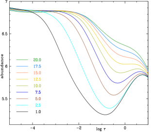
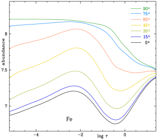
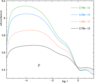
Figure 1: a) Stationary time-dependent chemical stratifications of Cr in magnetic fields of various absolute strengths (given in kG), inclined by $75\arcdeg$ with respect to the vertical. The stellar atmosphere is characterized by $T_{\rm eff}=12000$ K, $\log g=4.0$ and a mass loss rate of $8.5\times 10^{-15}$ solar mass per year. The curves show abundances normalized to $[H]=12.00$ vs. $\log\tau_{5000}$. b) Same stellar atmosphere, but stationary time-dependent chemical stratifications of Fe in a 17.5 kG magnetic field as a function of the angle with respect to the vertical. c) Stationary time-dependent chemical stratifications of P in the case of zero magnetic field as a function of the mass loss rate. The results pertain to a stellar atmosphere with $T_{\rm eff}=12750$ K and $\log g=3.7$.

2 Time-dependent atomic diffusion in the presence of magnetic fields

Ever since the ground-braking papers of Vauclair et al. (1979), Michaud et al. (1981), Alecian & Vauclair (1981) and of Babel & Michaud (1991a, b), there can be no doubt that the magnetic fields found in CP stars control the build-up of stratified abundances. It follows that the variation of inclination and of strength of the field over the stellar surface – be it simply bipolar or multipolar – will invariably lead to abundance inhomogeneities, both vertical and horizontal. In a series of papers, Alecian and Stift have modeled this process to an increasing degree of sophistication, starting with the effect of Zeeman splitting on accelerations Alecian & Stift (2002, 2004), translating accelerations to diffusion velocities (Alecian & Stift, 2006), establishing equilibrium solutions with zero particle flux (Alecian & Stift, 2007) and demonstrating what chemical stratifications would look like in a star permeated by a dipolar field (Alecian & Stift, 2010). The 3D-modeling of a star with a non-axisymmetric field geometry shows warped pseudo-rings of enhanced and depleted abundances, greatly varying with depth in the atmosphere (Alecian & Stift, 2017).

In another approach to diffusion in CP stars (Alecian et al., 2011), mass conservation is included in the calculations; iterations start from vertically constant abundances and continue until a stationary solution has been reached. Subsequent modeling with up to 7 chemical elements ranging from Ti to Ni showed how sensitively abundances depend on field inclination, even in the presence of quite moderate field strengths (Stift et al., 2013a; Stift & Alecian, 2016). A certain degree of self-consistency is achieved by updating the atmospheric model after a few iterations, a procedure that has also been applied to the equilibrium solutions. Finally, the last years have seen the introduction of mass loss which, not unexpectedly, has been shown to be able to greatly modify chemical stratification profiles (Alecian & Stift, 2019).

Being a slow process, atomic diffusion is very sensitive to mixing motions. The neglect of these in diffusion calculations is justified for ApBp stars where observations indicative of abundance stratifications confirm the assumed stability. On the other hand one cannot exclude that weakly turbulent layers may at times exist in these atmospheres and some physical processes are also missing in diffusion calculations such as for example NLTE effects – see Sec. 3 of Alecian (2015) for a non-exhaustive list of missing processes. Still, a number of general conclusions can be drawn from almost 4 decades of dedicated efforts at ApBp star atmospheres:

1. Atomic diffusion leads to vertical abundance inhomogeneities.

2. Horizontal magnetic fields of virtually any strength greatly influence the resulting stratification profile at various atmospheric levels – see e.g. Cr stratifications in fields of $75\arcdeg$ inclination (Figure 1a). Even a 1 kG field leads to an abundance increase by about 1 dex in the outermost layers.

3. From Figure 1a it is evident that weak fields play a role only in the upper layers. It needs strong fields to affect abundances deep in the atmosphere.

4. Field inclination has a greater effect on chemical stratifications in the outer layers than field strength

5. Abundance profiles cannot in general be approximated by the popular step function The Fe stratifications in a 17.5 kG field (Figure 1b) for example reveal the existence of cloud-like structures.

6. In magnetic CP stars with moderate to strong fields one cannot therefore expect any kind of globally constant chemical stratifications.

7. Mass loss modifies the vertical abundance profiles, suppressing diffusion almost completely at high mass loss rates – see the dependence on mass loss of the stratifications of phosphorus in a zero field case (Figure 1c).

All the stratifications shown in these figures and later ones in this paper have been obtained with the help of the CaratMotion code described by Alecian & Stift (2019). Based on the conclusions given above and on a wealth of further numerical results, we may now proceed to analyze some aspects of the (Zeeman) Doppler mapping approach to CP stars as practiced over the past 20 years.

3 Abundance mapping: assumptions and simple tests

There is no need to carry out another comparison of the respective virtues of the Tikhonov versus the maximum entropy functionals in the least-squares minimization problem at the basis of ZDM. Ever since the paper by Piskunov & Kochukhov (2002), (Zeeman) Doppler mapping of CP stars has been monopolized by the invers family of closely related codes, so that we may justifiably restrict our discussion to Tikhonov regularization and these codes. Thankfully, the numerous simplifying assumptions made in order to facilitate (and indeed to make possible) ZDM of magnetic CP stars have been laid out in detail by KP02. Chemical spots are characterized by vertically constant abundances, and invers sticks to this clearly unphysical approximation for all CP stars, even when in HD 3980 silicon seemingly becomes locally as abundant as hydrogen throughout an atmosphere whose overall temperature and pressure structure however is given by (much lower) abundances averaged over the star (Nesvacil et al., 2012). Stift et al. (2012) have shown that the use for spectrum synthesis of such mean atmospheres for every location on spotted stars, regardless of the actual local chemical abundances, can lead to serious errors in the recovered abundance maps.

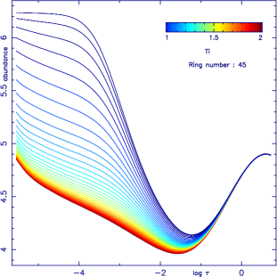
Figure 2: Same atmosphere as in Figure 1a,b. a) Chemical stratifications of Fe in the atmosphere of a star with a centered dipole of 2 kG polar field strength. Abundances along a meridian are color-coded according to the local field modulus and plotted versus the logarithm of optical depth. Same stellar atmosphere as in Figures 1a,b. b) Same as before but for Cr and a polar field strength of 15 kG. c) Same as before but for Ti and a polar field strength of 2 kG.

Fundamental physical questions are raised by results published for HR 3831 (Kochukhov et al., 2003a) with oxygen more abundant than hydrogen in an exceedingly small spot on and Ca locally almost as abundant as helium – remember that their oxygen and calcium spots stretch throughout the atmosphere unstratified. The problem of horizontal pressure equilibrium arising from the variations in the local atmospheric structure has never been addressed in ZDM studies, although one can immediately glean from published magnetic maps that in many places there is no strong vertical magnetic field that could possibly stabilize the local atmospheres (Stift & Leone, 2017a). Why have stratifications as established empirically for many CP stars since the 1990s – albeit assumed globally constant and mainly corresponding to step functions, see the comprehensive presentation by Ryabchikova (2014) – in no way entered the inversion procedure? No real simulations have ever been published as to how locally variable stratifications will influence ZDM results based on vertically constant local abundances. Kochukhov & Ryabchikova (2018) who constitute the sole exception only look at a simple centered dipole.

Apart from the restriction that abundances in spots be unstratified, the numerical tests devised for the mapping of abundance spots display a strange lack of sophistication as to the shapes of the horizontal abundance inhomogeneities assumed in Kochukhov & Piskunov (2002) and in Kochukhov (2017). Just look at the Si, Cr and Fe maps of $\alpha^{2}$CVn (Kochukhov et al., 2002), published almost simultaneously in the same series of papers. A star featuring 2 or 3 high-contrast spots of vertically constant abundance, well distributed in both longitude and latitude, is an entirely artificial construct and there is no guarantee nor is it even likely that it would correspond to what one has to expect, even if exact theory were involved. Neither does this constellation of spots bear the remotest resemblance to the numerous abundance maps of $\alpha^{2}$CVn published over the years, even less so to the Ca and Fe maps of HR3831 (Kochukhov et al., 2004b). In KP02’s original tests, only 2 abundance values were involved, in this respect very similar to the black and white values in the famous “Vogtstar” example. The latter however is much more complex, consisting of 4 letters with fine structure that Kochukhov’s spots are completely lacking. Still, despite adopting inclination, rotation, magnetic geometry, etc. that are optimum for Doppler mapping, the results are somewhat disappointing. A close look (better in color, not B/W) reveals that the quoted average error of 0.04 dex is meaningless, reflecting a very specious statistical Ansatz; spurious structures attain amplitudes of up to $\pm 0.5$ dex. To summarize, the tests of ZDM presented so far are based on artificial scenarios where diffusion is absent, spots are of high contrast, small in number, largish, perfectly symmetric and well distributed in longitude and latitude. In other words, they are entirely alien to the complex world of magnetic CP stars.

4 1D to 3D regularization in magnetic CP stars: abundances and magnetic fields

The indiscriminate use of physics-free regularization in the analysis of CP stars can lead to strange results, even outside the strict realm of ZDM. In their attempt to determine global 1D stratifications of chemical elements in the atmosphere of HD 133792, Kochukhov et al. (2006) claimed to have devised a technique that “for the first time allowed us to recover chemical profiles without making a priori assumptions about the shape of chemical distributions.” The Tikhonov approach chosen for the analysis of HD 133792 minimizes the sum of the squares of the vertical abundance gradients with optical depth, a purely mathematical constraint which can easily be shown to have nothing to do with theoretically modeled chemical stratifications in a magnetic CP star. Look for example at the stratifications predicted for simple centered dipoles of 2 kG and 15 kG polar strength respectively. Based on a grid of chemical profiles for field strengths from 1 kG to 20 kG and field directions from vertical to horizontal, one can establish the vertical abundance structure along a meridian (for a dipole aligned with the rotational axis) or the equator (for a dipole lying in the equatorial plane) as plotted in Figures 2a,b,c. Even in the case of a low contrast, weak field – the field modulus ranges from 1 to 2k̇G – Fe abundances in the upper layer diverge by more than 1 dex. As expected, we see a much greater effect reaching 2 dex for Cr in fields ranging from 7.5 to 15 kG. If one can discern anything bearing resemblance to a “transition region” between low and high abundances in the Cr stratifications, its extension, shape and slope greatly varies all along the meridian, at variance with the assumptions underlying the 3D regularization functional used by Rusomarov (2016) (see below). It becomes immediately obvious that the adoption of a globally constant vertical abundance profile in the analysis of HD 133792 disregards the complex astrophysical reality. From a comparison between our Figures 2a,b,c and Figures 3 and 5 of Kochukhov et al. (2006) it also transpires that in stark contrast to the assertions made, completely unphysical a priori assumptions have silently been introduced, concerning the shape of the chemical distributions, viz. a very special kind of smooth step function which asymptotically reaches the solar abundance both in the deepest and in the outermost layers. See Stift & Alecian (2009) for further discussions.

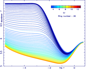
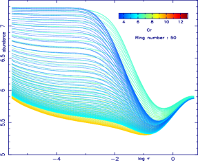
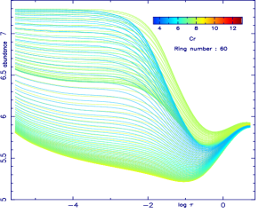
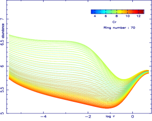
Figure 3: Chemical stratifications of Fe in the atmosphere of a star with a magnetic geometry similar to that of HD 154708. The stratification profiles are color-coded according to the local field moduli which range between 3.35 and 12.89 kG; they are plotted versus the logarithm of optical depth. Ring numbers 20, 30, 40, 50, 60, and 70 correspond to latitudes $-50\arcdeg$, $-30\arcdeg$, $-10\arcdeg$, $+10\arcdeg$, $+30\arcdeg$, and $+50\arcdeg$. Same stellar atmosphere as in Figure 1a,b

.

Both in the mapping of 2D horizontal abundance maps and in the derivation of vector magnetic field maps of CP stars, Tikhonov regularization is presently the only constraint in use. Unlike the “Vogtstar” case which is conveniently devoid of physical meaning, stratified abundances are governed by processes involving magnetic fields (have a look again at Figures 2a,b,c), but this is not reflected in the functionals employed in the invers family of codes. Kochukhov & Wade (2010) give one example in their eq. (5), where they minimize simultaneously the double sum of the squared differences between all combinations of 2 magnetic vectors and all combinations of 2 abundances of the chemical elements considered in the inversion. One would be hard pressed to devise a more arbitrary and less physically motivated, yet mathematically expedient regularization: neither does it take into account the properties of truly multipolar field geometries – not just dipole or dipole plus quadrupole – nor does it in the least reflect the dependence of chemical stratifications on field direction and field strength. There are no tests to be found in the literature that would demonstrate how this regularization could possibly ensure the correct recovery of a magnetic field with poloidal and toroidal components of spherical harmonics degree and order of 10 or more. Let us recall that the tests presented by KP02 deal exclusively with a dipole of 8 kG (!) polar strength and a few models with an added axisymmetric quadrupole, of 8 kG strength again. Tests based on these huge field strengths and devised in a way that “magnetic geometry, rotational velocity and inclination collaborate to maximize the magnetic variability of the spectral line profiles and represent an ideal combination for the application of MDI” cannot provide answers to this question.

Without further discussion, Kochukhov et al. (2014) have introduced a new penalty function in the context of inversions where spherical harmonics are fitted to the observed magnetic field. They chose the expression $\Sigma_{l,m}~{}l^{2}\,(\alpha^{2}+\beta^{2}+\gamma^{2})$ where $\alpha,\beta$ and $\gamma$ characterize contributions of the radial poloidal, horizontal poloidal, and horizontal toroidal magnetic field components, respectively. Again, there are neither tests nor theoretical considerations to show that this particular penalty function would ensure correct magnetic maps. A mere 2 years later, Rusomarov et al. (2016b) presented yet another penalty function $\Sigma_{l,m}~{}l^{2}\,(\alpha+\beta+\gamma)^{2}$; this surprising change was not accompanied by a single argument nor was it buttressed by tests similar to those published by KP02. This leaves the world with at least 3 penalty functions, all of which constitute largely or even entirely untested ad hoc constructs. We will demonstrate later in this paper that these penalty functions fail to lead to physically feasible field geometries in strongly magnetic CP stars. This failure likely extends to weak-field CP stars.

The application of Tikhonov regularization to 2D abundance maps neglects the undisputed fact that stratifications are related to the local magnetic field. Figure 3 reveals the diversity of chemical profiles in a star with a magnetic field geometry similar to that of HD 154708 (Stift et al., 2013b). ZDM in its present form tries to fit integrated line profiles (originating from vertically and horizontally varying stratifications) to integrated line profiles assumed to emanate from horizontally varying but vertically constant abundance profiles. At the same time the unstratified profiles forced onto the vertically variable profiles have to conform to the artificial restraint of minimum horizontal abundance gradients. Only simulations based on theoretical stratifications could give us hints as to the interpretation of the results of such a procedure.

4.1 3D abundances and an improper regularization

Kochukhov et al. (2009, JD4 @ IAU GA XXVII) and later Rusomarov (2016) in section 2.3 of his PhD thesis – submitted as Rusomarov et al. (2016a) to A&A but never accepted for publication in any journal – attempted to derive 3D abundance profiles of Fe in the atmospheres of $\Theta$ Aurigae and of HD 24712 respectively. In spite of what had already been known for some time about stratifications in Ap star atmospheres (see e.g. Alecian & Stift 2010), Rusomarov adopted the regularization scheme previously devised by Kochukhov that minimizes all possible differences between the totality of idealized local stratification profiles; for numerical convenience the latter are assumed to be step-like. In the Kochukhov-Rusomarov picture, the depth-dependence of the abundance profiles is a function of 4 parameters: abundance in the upper atmosphere $\epsilon_{\rm up}$, abundance deep in the atmosphere $\epsilon_{\rm low}$, position $d$ and width $\delta$ of a transition region lying somewhere in between. From these 4 parameters, 5 quantities are formed whose square sums are minimized simultaneously, viz. $\Sigma\,|\Delta\epsilon_{\rm up}|^{2}$, $\Sigma\,|\Delta\epsilon_{\rm low}|^{2}$, $\Sigma\,|\Delta\,d|^{2}$, $\Sigma\,|\Delta\delta|^{2}$, $\Sigma\,(\epsilon_{\rm up}-\epsilon_{\rm low})^{2}$. No theoretical basis is offered for this particular regularization, neither in section 2.3 of the thesis nor in the A&A submission. One also acutely misses tests that would show how and under which conditions the proposed ZDM approach could be able to recover complex 3D chemical profiles as for example predicted by diffusion theory. Instead of finding a carefully devised, executed, described and discussed set of tests we are faced with a simple (unspoken) extension to the old KP02 belief “that the code can be successfully applied to the imaging of global stellar magnetic fields and abundance distributions of an arbitrary complexity”. Apparently the exact form of regularization functionals used in ZDM does not matter and therefore does not have to be argued; whenever regularization is presented to the astronomical community as Tikhonov-like, it seemingly is expected to be accepted without further questioning.

The approach chosen by Kochukhov and by Rusomarov is clearly at variance with the diffusion models of Alecian & Stift (2007) which show that chemical profiles strongly depend on magnetic field direction and strength. This holds true not only for equilibrium solutions but also for the more realistic time-dependent results, even though the final stationary solutions may deviate from the solar abundances adopted at the start of the calculations in a sense opposite to what is found for equilibrium solutions (Stift & Alecian, 2016). Figures 2a,b,c have already revealed that one is faced with considerable variations of $\epsilon_{\rm up}$ but also in the position $d$ and width $\delta$ of the transition region in a field geometry as simple as a centered dipole, even at fairly modest field strength. Much enhanced variations are found in another geometry of rather moderate complexity, illustrated by Figure 3. With local field moduli ranging between 3.35 and 12.89 kG, this allegedly “unspecified eccentric dipole with an unusually high contrast” (in fact representing the magnetic geometry of HD 154708) – a mere factor of 3.8 as compared to 5.6 derived for HD 32633 by Silvester et al. (2015) and a staggering 11.5 for HD 119419 according to Rusomarov et al. (2018) – helps to convey a reasonably conservative estimate of how non-homogeneous, strong magnetic fields can lead to an impressive variety of chemical stratifications over the stellar surface.

From these plots and from stratifications predicted for many other geometries it follows that forcing artificial uniformity onto idealized local step-functions and then minimizing abundance differences at all costs cannot possibly provide valid insights into the physics of CP stars. The very peculiar, arbitrary and physics-free regularization functional first chosen by Kochukhov and later taken up again by Rusomarov cannot but lead to spurious solutions for the abundances, disconnected from the true magnetic geometry. Such abundance maps rather imply an unnatural magnetic geometry featuring small differences in field strength and even smaller differences in field angle; they are entirely free from any physical meaning,

5 Magnetic fields of CP stars, through Maxwell to Alfvén

In the first ZDM mapping of a CP star based on all 4 Stokes parameters, Kochukhov et al. (2004a) derived a vector magnetic field map of 53 Cam, revealing absolute field strengths over the stellar surface ranging from 4 to 26 kG. Checking the consistency of their map with Maxwell’s equations, they found a large (44%) magnetic flux imbalance. It is hard to understand why 53 Cam has never been reanalyzed in subsequent years – in contrast to other stars first studied in the earliest days of ZDM such as $\alpha^{2}$ CVn or HD 24712 – despite these shortcomings and despite the fact that present-day spectrographs would provide observational material of much higher resolution and signal-to-noise ratio. At present the true surface structure of 53 Cam must thus be considered unknown.

In a later study, Kochukhov & Wade (2010) failed to provide details as to a possible magnetic flux imbalance for $\alpha^{2}$ CVn. The approximation of their vector magnetic map with spherical harmonics appears to be more satisfactory than for 53 Cam, but the size of the deviation from zero divergence of the discrete map remains unspecified. A better situation seems to prevail for HD 32633 (Silvester et al., 2015), a star with a mean field modulus of about 8 kG. In the magnetic field inversion based on all 4 Stokes parameters, the invers code was allowed to fit harmonics up to $l=10$, including poloidal and toroidal components. The radial and the horizontal poloidal field components were determined separately, i.e. the coefficients $\alpha_{\rm lm}$, $\beta_{\rm lm}$, and $\gamma_{\rm lm}$ of the spherical harmonics expansion specifying the field geometry were allowed to vary independently as in Kochukhov et al. (2014).

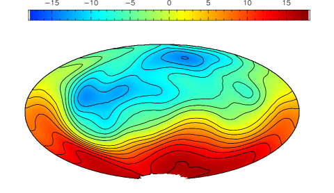
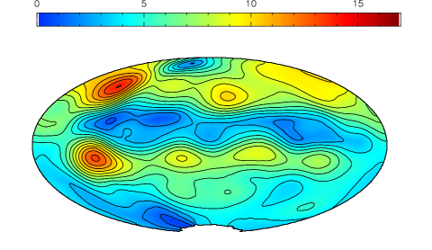
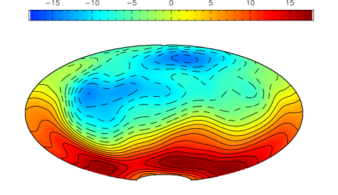
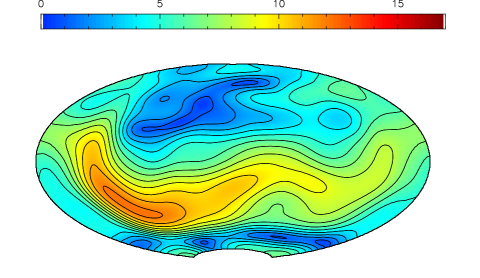
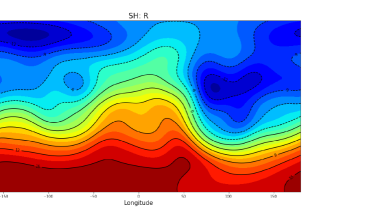
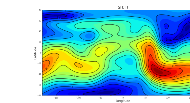
Figure 4: a) Radial magnetic field of HD 32633 (left). From top to bottom : original field recovered from published plots, original field fitted with spherical harmonics, original field fitted with an independent code by C.D. Beggan (British Geological Survey, Edinburgh). The phases differ by $180\arcdeg$ between the two codes. b) Horizontal magnetic field of HD 32633 (right). From top to bottom: original field recovered from published plots, horizontal field derived from the radial field by assuming a potential poloidal force-free configuration, horizontal field derived similarly with the independent code by C.D. Beggan.

Enter Hannes Alfvén and magnetohydrodynamics. It is well known that in the solar corona magnetic structures have to be force-free, $(\nabla\wedge B)\wedge B=0$, given the dominance of Maxwell stress and/or magnetic pressure over gas pressure. Force-free fields are also prominent in the solar chromosphere and they govern the structure of sunspots (see e.g. Tiwari 2012). The vertical magnetic fields of sunspots only very rarely attain values of 4 kG, so shouldn’t the field of HD 32633 with regions of up to 17 kG field strength as derived by Silvester et al. (2015) also qualify as force-free? Spruit (2017) answers this in the affirmative and also points out that the construction of a force-free field is not possible in terms of a boundary-value problem; force-free fields must be understood in the context of the entire history of the fluid displacements at their boundary. It follows that within the framework of ZDM it is not possible to determine the shape of a force-free configuration; the inversion of strong magnetic fields in CP stars must needs be based on purely potential fields, ensuring $\nabla\wedge B=0$ in addition to zero divergence.

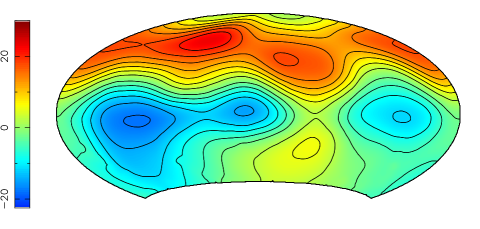
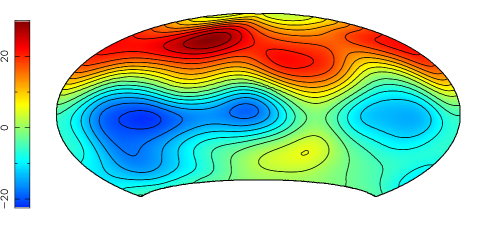
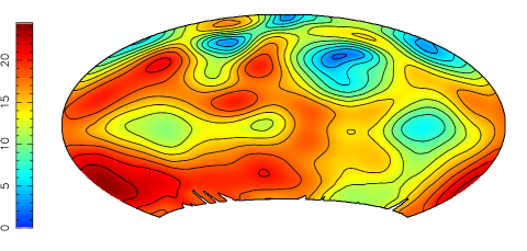
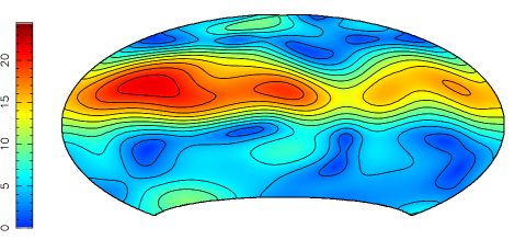
Figure 5: a) Original radial and horizontal magnetic field of HD 119419 (left, top to bottom). b) Corresponding force-free radial and horizontal magnetic field (right, top to bottom).

Writing down $\nabla\wedge B=0$ in spherical coordinates leads to eqs. (12)-(14) of Kochukhov et al. (2004a) with all 3 components of the current $J$ set to zero. These equations define the relation between the components of the magnetic field vector. Since $B_{r}$ depends on $B_{\phi}$ and on $B_{\theta}$, it is not legitimate to determine $\alpha_{\rm lm}$ independently from $\beta_{\rm lm}$ and $\gamma_{\rm lm}$. Eqs. (1)-(3) of Kochukhov et al. (2014) can possibly be applied to very weak fields, but certainly not to stars like HD 32633 (Silvester et al., 2015), 53 Cam (Kochukhov et al., 2004a), HD 75049 (Kochukhov et al., 2015), HD 119419 (Rusomarov et al., 2018), HD 125428 (Rusomarov et al., 2016b), HD 133880 (Kochukhov et al., 2017) and probably also not to 49 Cam (Silvester et al., 2017) and $\alpha^{2}$ CVn (Silvester et al., 2014a). In view of the field strengths observed, it perspires that all Zeeman Doppler maps of CP stars with strong fields have been obtained with an incorrect set of formulae. The published magnetic maps for the above-mentioned CP stars are therefore all entirely spurious, and so are all the abundances, since Zeeman splitting, Zeeman intensification and polarization of the spectral lines are based on erroneous magnetic field values. The situation is not quite so clear-cut with stellar fields of more moderate strength but as Spruit (private communication) points out, these are probably also stable on very long time scales so that Ohmic diffusion has given the field in the atmosphere sufficient time to relax to its lowest energy state, viz. a potential field.

5.1 Published vs. force-free maps

Geophysicists modeling the earth’s magnetism do not restrict the dissemination of their results to colorful plots in journals and on web-pages, rather they provide extensive tables, Fortran codes with hundreds of lines of data, notebooks, etc… This allows fellow scientists to take advantage of the existing wealth of models for further investigations; it also constitutes a useful check on the integrity of data and models. No openness of this kind is encountered in ZDM, quite to the contrary not even the coefficients of the spherical harmonics expansion of any of the many CP stars analyzed has ever been made available apart from those for 36 Lyn (Oksala et al., 2018). Over the years, there has been no way to obtain ZDM data in view of an independent assessment of the published maps and of further analyses. Among others, this inaccessibility of the ZDM data precludes the prediction (by scientists working on atomic diffusion) of observable Stokes profiles, based on theoretical field-dependent chemical stratifications unless close supervision is accepted. Kochukhov verbatim: “I provide access to my DI methods in the context of collaborative projects, in which I am involved at all stages from problem formulation to eventual publications. In most cases I compute DI maps myself using the data files prepared by collaborators.” Being in themselves legitimate, these wide ranging restrictions have led to the scientifically highly undesirable situation that not only the ZDM maps, but even the methods leading to these maps, have largely remained unassailable over the years – for the few exceptions see e.g. Stift (1996), Stift et al. (2012), Stift & Leone (2017b, a).

Fortunately, things have changed recently, although neither journal editors nor referees have insisted at last on making ZDM data routinely available. A few transformations applied to the published ZDM maps suffice to recover magnetic field geometries to a gratifying degree of reliability. Figure 4a (top) shows the radial field of HD 32633 as reconstructed from the maps published by Silvester et al. (2015), Figure 4b (top) the horizontal field. Below to the left we show a spherical harmonics fit with $l=1-9$ applied to the recovered map of the radial magnetic field. The excellent agreement with the original plot is quite surprising, given the many steps involved in the reconstruction. For all practical purposes, the data underlying the Hammer projections in these plots are near enough to the results obtained with the invers10 code to be used straightforwardly in further analyses. We know that in the case of potential poloidal (and thus force-free) fields, the horizontal field components can be derived directly from the radial field (see e.g. Winch et al. 2005). For the necessary calculations we have developed a new code, testing it with the International Geomagnetic Reference Field (Alken et al., 2021). We note that the resulting map (Figure 4b middle) of the horizontal field – force-free as required in view of the strong magnetic fields involved – is totally at variance with the original map which represents a non-potential field with magnetic forces that are not in balance. In an independent analysis of the original magnetic maps, C.D. Beggan (British Geological Survey, Edinburgh) has confirmed that from the raw published radial field maps, one cannot reproduce the horizontal or modulus plots shown in the paper (bottom of Figures 4a,b).

We also had a look at HD 119419 (Rusomarov et al., 2018) with its magnetic field modulus reaching about 26 kG and its spectacular 4 “spots” of very low values of the horizontal field. Strangely, here the spherical harmonics fit to the radial field is somewhat unsatisfactory, the residuals being almost 3 times as large as for HD 32633. Although we feel unable to explain this discrepancy, Figure 5a shows a field map sufficiently near to the original one about the equator and in the northern hemisphere to make possible the desired further analyses. Proceeding as for HD 32633 with our well tested code, we show that the published horizontal field certainly is not force-free (Figure 5b).

Similar analyses should prove straightforward for HD 125428 (Rusomarov et al., 2016b) and HD 133880 (Kochukhov et al., 2017). In the case of HD 75049 (Kochukhov et al., 2015), on account of the low inclination $i=30\arcdeg$, it will be much more difficult to obtain the direct proof of a violation of the force-free condition despite the extreme field strengths involved. It is however already amply clear that the Tikhonov regularization functional applied in the analysis of HD 32633 and of HD 119419 does not lead to solutions that are physically – instead of merely mathematically – feasible. It comes as a serious blow to the credibility of ZDM that for CP stars with strong fields, it routinely converges to physically impossible magnetic geometries and corresponding completely spurious abundance maps, while displaying good or excellent fits to the observed Stokes IQUV profiles. No doubt, we are faced with particularly obnoxious instances of non-unique inversion results.

6 Ever changing maps

Regularization and force-free fields are not the only problem facing ZDM. The permanent changes of magnetic and abundance maps pervading the literature are equally worrisome. Let us start with 53 Cam which has been observed in all 4 Stokes parameters just once, but analyzed and reanalyzed at least 5 times with widely different results for the magnetic field modulus (Table 1). Contrasts range from 21.9 to 29.5 kG, minimum field strengths from 1.4 to 4.0 kG, and maximum field strengths from 25.1 to 32.3 kG; At the same time, still based on the same data set, abundance contrasts for Si and Fe change by about 1 dex; $\Delta\epsilon$(Si)$=3.4$ dex and $\Delta\epsilon$(Fe)$=4.0$ dex (Kochukhov et al., 2004a) become $\Delta\epsilon$(Si)$=4.3$ dex and $\Delta\epsilon$(Fe)$=5.0$ dex (Piskunov, 2008). All these changes are far outside the error limits of ZDM claimed by Kochukhov (2017).

53 Cam is not an isolated case. $\alpha^{2}$CVn has been observed and analyzed a number of times and there are at least 9 different magnetic geometries to be found in the literature (Table 2). The field modulus contrasts range between 2.5 and 6.3 kG. the minimum field strengths between 0.0 and 1.4 kG, and the maximum field strengths between 3.1 and 7.7 kG, a factor of 2.5 ! Earlier magnetic mappings based on Stokes $IV$ had determined dipolar plus quadrupolar contributions of $B_{\rm d}=5.3$ and $B_{\rm q}=1.5$ kG (Kochukhov et al., 2001), soon to be replaced by $B_{\rm d}=6.18$ and $B_{\rm q}=1.08$ kG (Kochukhov et al., 2002). These impressive discrepancies in the magnetic field are accompanied by substantial changes in the recovered abundance contrasts: from 2.4 dex to 4.0 dex (Si), from 4.8 to 3.0 dex (Cl), from 1.8 dex to 4.0 dex (Ti), from 2.3 to 3.5 dex (Fe), and from 2.0 to 4.0 dex (Nd). Since the abundances have always been derived simultaneously with the magnetic field, it would seem that only the neglected local atmospheric structure can be considered responsible if one followed the arguments of Kochukhov (2017). Abundance changes of 2 dex and more however are in complete contradiction to his claims that ignoring the varying local atmospheres leads to average reconstruction errors of $\approx 0.2$ dex and maximum errors of $\approx 0.3$ dex and that the invers code achieves an overall average accuracy of 0.06–0.09 dex and maximum errors of 0.12 dex. The conclusion is inevitable that there must be other sources of errors than those discussed by Kochukhov (2017).

Table 1: Magnetic field moduli for 53 Cam.

$B_{\rm min}$ [kG]	$B_{\rm max}$ [kG]	Reference
2.8	32.3	(Piskunov & Kochukhov, 2003)
3.8	28.2	(Kochukhov et al., 2003b)
4.0	25.9	(Kochukhov et al., 2004a)
1.4	26.1	(Kochukhov, 2004)
1.5	25.1	(Kochukhov, 2007)

Note. — Moduli determined from the same set of Stokes $IQUV$ observations.

May we mention at this point that for another frequently observed and analyzed star, HD 24712, abundances are beset by similar problems. Lüftinger et al. (2010a) have claimed a Nd contrast of 1.1 dex; although in a later study it is stated that “the new maps confirm the previous findings, and also show some details the previous study lacked” (Rusomarov et al., 2015), it emerges that not only does the Nd contrast increase to 2.6 dex, but the spot even changes position from about $-25\arcdeg$ south to near $-75\arcdeg$ south! Finally, it is worthwhile to have a look at HR 3831 where the same set of observations has led to sometimes widely different abundance maps – keep in mind that the magnetic field was not determined, but simply assumed dipolar and subsequently disregarded in the Doppler mapping procedure. Putting aside the insoluble problem of the structure of a hypothetical atmosphere in a spot with oxygen more abundant than hydrogen (Kochukhov et al., 2003a) and its equilibrium with the rest of the atmosphere where oxygen can be some 7 dex (!!) less abundant, we note a 2.0 dex difference in the maximum abundance of Ca between Kochukhov et al. (2003a) and Kochukhov et al. (2004b), of 1.3 dex for both Li and Eu, and an almost complete dissimilarity between the respective Si maps.

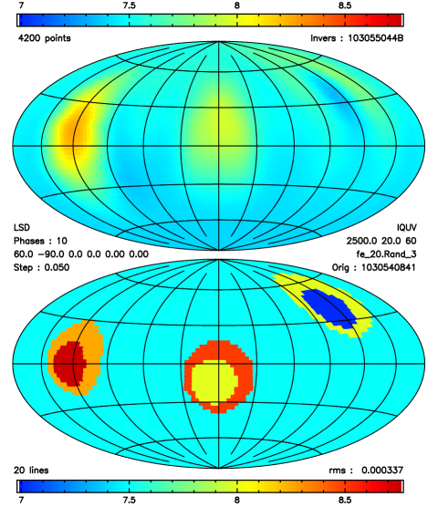
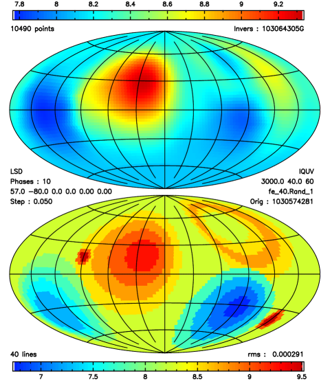
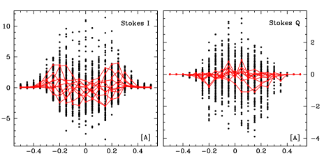
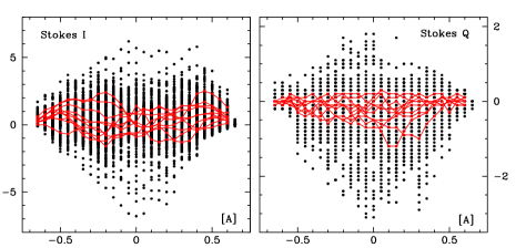
Figure 6: LSD based ZDM results for 2 different assumed horizontal abundance distributions with a stellar atmosphere characterized by $T_{\rm eff}=9000$ K, $\log g=4.0$ and vertically constant chemical abundances. a) Original and inverted abundance map based on 20 lines (left, middle and top) for a dipolar field with obliquity $90\arcdeg$ and polar strength $B_{\rm p}=5$ kG. Inclination $i=60\arcdeg$, $v\,\sin i=20\,{\rm km\,s}^{-1}$, wavelength resolution 50 m${\AA}$, 4500 pixel spatial grid. Bottom: residuals calculated minus “observed” (in units of $10^{-3}$) for individual line profiles (black dots) and mean profiles (red line). b) Original and inverted abundance map based on 40 lines (right, middle and top) for a dipolar field with obliquity $80\arcdeg$, $B_{\rm p}=6$ kG, $i=57\arcdeg$, $v\,\sin i=40\,{\rm km\,s}^{-1}$. Same spectral resolution and same spatial grid. Bottom : same residuals as before.

Table 2: Magnetic field moduli for $\alpha^{2}$CVn.

$B_{\rm min}$ [kG]	$B_{\rm max}$ [kG]	Spectra	Reference
1.4	7.7	$IV$	(Kochukhov et al., 2003b)
1.0	4.3	$IQUV$	(Kochukhov, 2004)
0.6	3.1	$IQUV$	(Kochukhov, 2007)
0.0	4.4	$IQUV$	(Kochukhov & Wade, 2010)
0.1	4.9	$IQUV$	(Silvester et al., 2014b)
0.0	5.5	$IQUV$	(Silvester et al., 2014c)
0.5	4.5	$IQUV$	(Kochukhov, 2018)

The apex of unexplained published abundance differences is reached for $\kappa$ Psc. Ryabchikova et al. (1996) finds Cr abundances between -6.08 and -3.42 whereas according to Piskunov et al. (1998) these values become -6.09 and +0.27, making Cr almost twice as abundant than hydrogen! The authors do not agree either on inclination or gravity, $i=35\arcdeg$ and $\log g=3.75$ being the choice of Ryabchikova et al. (1996), Piskunov et al. (1998) adopting $i=70\arcdeg$ and $\log g=4.50$. The absurd consequence of a Cr abundance twice that of hydrogen would be a pressure scale height in the spot that is about 30 times smaller than in the rest of the atmosphere. Translated to our planet, the pressure on top of Heaval (Barra, Outer Hebrides, 383m) would lie below the pressure on top of Mt. Everest (8848m). How could such a huge pressure difference remain stable for days, weeks, years or centuries, even when separated by whole continents?

7 LSD

Least-squares deconvolution (LSD) (Donati et al., 1997) was devised for the detection of weak magnetic signals in noisy spectra. Its usefulness for this particular purpose remains undisputed, although extreme care has to be taken for the conversion of a LSD signal to quantities such as for example $B_{\rm eff}$, the integrated longitudinal field of a magnetic star (see Scalia et al., 2017; Ramírez Vélez, 2020). A lack of extended, realistic tests makes it as yet impossible to assess whether the use of LSD mean profiles in ZDM as carried out by Kochukhov et al. (2014) leads to valid stellar maps. Please keep in mind that LSD based ZDM is just one special instance of single-line inversions which only for highly idealized cases have been shown to result in unique solutions. Stift & Leone (2017a) for example have demonstrated that one is frequently/usually faced with multiple solutions even in the total absence of photon noise and despite almost perfect fits to the observed profiles. The use of LSD profiles in ZDM of course drastically lowers the observational noise, but unfortunately this is done at the expense of the information contained in the various spectral lines (different strengths, Zeeman patterns, …).

To see what can happen, let us have a look at a star featuring 2 medium-size spots featuring each 2 abundances, and 1 ring-like structure. Adopting an inclination of $i=60\arcdeg$, a centered dipole normal to the rotational axis with polar strength 5.0 kG and a projected rotational velocity of $v\,\sin i=20\,{\rm km\,s}^{-1}$, we synthesize spectra for 20 unblended lines at 10 equidistant phases at a wavelength resolution of 0.050 Å and spatial resolution of $\approx 4500$ surface pixels. The subsequent inversion – based on all 4 Stokes $IQUV$ parameters – is carried out under the assumptions that the stellar parameters like temperature, gravity, magnetic field etc., but also the atomic parameters, are exactly known. The only unknowns are the horizontal variations of the chemical abundance (taken vertically constant) of a single element. There are thus some 4000 unknowns to be derived from the phase-dependent $IQUV$ profiles of a single mean line; for each of the 10 phases, the mean line results from 4100 individual contributions in $IQUV$. Despite the large number (16800) of profile points, thanks to LSD we are faced with a classical, heavily underdetermined inverse problem which has to be solved based on a mere 840 mean profile points. We follow the approach of Kochukhov et al. (2014) and make the fit to the observed LSD profiles with the help of mean profiles determined at each iteration step from the individually synthesized spectral lines. It is thus not assumed that the LSD profiles display the behavior of a hypothetical single spectral line with some ill-defined mean parameters. Although the fit to the observed LSD $IQUV$ profiles is good to a few $10^{-4}$, Figure 6a (top and middle) reveals a disappointing map that indicates the presence of 2 low-contrast spots, giving also a marginal hint at a possible ring-like structure, but failing outright to yield correct abundances. The minimum abundance is overestimated by 0.33 dex, the maximum abundance underestimated by 0.50 dex so that the original 1.75 dex contrast is almost halved to 0.92 dex !

In another test, we worked with a star featuring 5 structured spots of varying size and 1 large ring-like structure. Adopting inclination and obliquity of the centered dipole similar to those of the former model, we increased the polar magnetic field strength to 6.0 kG, the projected rotational velocity to $v\,\sin i=40\,{\rm km\,s}^{-1}$ and the number of spectral lines to 40. LSD reduces the resulting $42\,000$ profile points to 1040, leading to an abundance map which essentially recovers only the strongest spot at $+19\arcdeg$ despite a fit that is again good to a few $10^{-4}$ (Figure 6b, top and middle). All three southern spots would remain invisible unless one uses different color scales for original and ZDM map respectively as in this plot. Thanks to the chosen color scales one can see that the abundances in the 2 large southern spots are overestimated by up to 1 dex, and that the small overabundant spots at $-40\arcdeg$ and $+17\arcdeg$ do not show up at all. In addition, we note that the underabundant southern spots shift from $-32\arcdeg$ to $\approx-14\arcdeg$ and from $-33\arcdeg$ to the equator.

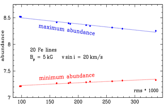
Figure 7: Recovered abundance contrast as a function of the rms scatter of the fit to the 4 Stokes LSD profiles.

A detailed analysis of the mean ZDM profiles and the profiles of the individual lines reveals the disturbing fact that some kind of numerical compensation mechanism can ensure almost perfect fits between input and modeled mean LSD Stokes profiles, although the fit to the individual spectral lines may be quite bad. This is demonstrated in Figure 6a (bottom) where we have plotted the differences calculated minus “observed” (input) for the individual line profiles (black dots) and for the mean profile (red line), both in Stokes $I$ and $Q$. It has to be emphasized that these differences, exceeding 1% of the continuum in Stokes $I$, do not represent observational errors but are entirely due to incorrect ZDM abundance maps. As we can see, it happens that individual lines are affected in different ways and that errors thus compensate, leading to excellent mean fits as in the Stokes $Q$ example. Our second model displays quite similar behavior, Stokes $Q$ being particularly instructive (Figure 6b, bottom).

Is there any information left in the mean Stokes profiles which would allow us to correctly recover the spots in Figure 6a and their true abundances? We think that we can confidently state that this information has not been destroyed in the LSD procedure, but that in real life it remains inaccessible. Figure 7 shows how in the course of the ZDM iterations the inverted minimum and maximum abundances change with the quality of the fit. At a rms scatter of the fit of $3.37\times 10^{-4}$, the 2 spots are only poorly recovered and the ring-like structure hardly recognizable. Not before the rms scatter has come down to $9.7\times 10^{-5}$ does the LSD-ZDM inversion start to yield an abundance map that resembles the input map, but the contrast of 1.3 dex is still far from the original 1.75 dex. In other words, even fitting observed Stokes profiles to an accuracy of $10^{-3}$ or a few $10^{-4}$ will not suffice to glean information on this simple surface structure.

From these results it transpires that LSD based ZDM makes the traditional problem of single-line inversions even less tractable: the code now can achieve an almost perfect fit to the mean observed profiles by summing up over individual profiles which may largely be incorrect. One can encounter at least 3 major situations:
1) The fit to the LSD profile is excellent, but differences between the synthetic and the observed individual spectral lines are much larger. The resulting map is in error because LSD has introduced many additional degrees of freedom so that it becomes more likely that ZDM converges to spurious and unphysical solutions (as in Figure 6a).
2) Both the fits to the individual spectral lines and to the LSD profiles are excellent but the resulting map is entirely at variance with the input map (as in Figure 6b).
3) All fits are excellent and the final map is correct.
Unfortunately, case 2) implies that even an almost perfect fit to all 40 lines individually can result in a spurious map. We do not at present see how it would be possible to discern between 2) and 3) in a LSD based ZDM inversion.

8 Conclusions

In the previous sections we have looked closely at the regularization employed by the invers family of codes for ZDM of CP stars, both regarding the vector magnetic field and the abundance inhomogeneities. Whether chemical profiles are assumed variable in depth but horizontally homogeneous, or taken to correspond to step-like functions that can change in all three dimensions, the verdict is clear: the regularization functionals proposed by Kochukhov and collaborators do not in the least reflect anything we know about the physics of the atmospheres of magnetic CP stars or of our Sun.

In the past, the magnetic geometries as derived from Stokes $IV$ observations or later from high resolution and high signal-to-noise ratio Stokes $IQUV$ line profiles have escaped close scrutiny. Although the published maps for 53 Cam did not fulfill the condition of zero divergence, there never was a reassessment based on new observations. Later analyses of strongly magnetic BpAp stars took more care to ensure zero divergence by fitting spherical harmonics to the magnetic vector field, but as we have shown, the formulae used are incompatible with force-free fields. Looking at the huge differences between the published horizontal field maps and the horizontal fields derived from the radial maps, there can be little doubt that all these published abundance maps have to be discarded.

The ever-changing magnetic and abundance maps for several well observed and well analyzed magnetic CP stars are not apt either to increase our confidence in the alleged accuracy of ZDM inversions.There are also those alleged low-contrast Cu and Ni spots in HD 50773 (Lüftinger et al., 2010b) that can be shown to exhibit spectral signatures completely swamped by the noise of the observed spectra (Stift & Leone, 2017b). On the other side, when O, Si, or Cr are claimed to be more abundant than hydrogen, and other metals like Mn and Fe almost as abundant as helium, how could these spots ever stay in equilibrium with the surrounding atmosphere? How could such extreme local atmospheres be treated correctly both physically and numerically?

In view of the results obtained in the course of this study, the bleak outlook for ZDM presented by Stift & Leone (2017a) appears to have become hopeless. The problem of a regularization functional that would reflect the physics of stratified magnetic CP star atmospheres admits of no solution. We are faced with a 3D problem of horizontal pressure and vertical hydrostatic equilibrium that cannot be adequately approximated by a 1D or 2D approach involving isolated “cylinders” characterized by some magnetic field vector. In the course of time, abundance gradients build up in each “cylinder” – depending on the local field strength and angle – density, pressure and temperature of the local atmosphere change differently in each “cylinder”, but what happens with the ensuing horizontal differences in gas pressure? Equilibrium must be reached on the shortest of time scales between one “cylinder” and all its neighbors, not just the nearest. A strong vertical field may help to stabilize the “cylinders”, but nearly horizontal field lines will not do so. It is inconceivable, even with the most sophisticated codes and the most powerful supercomputers, to simulate the field-dependent build-up in time of hundreds or thousands of vertical abundance profiles, and their global, 3D horizontal interaction during or after each time step, once again as a function of the local magnetic field vector. It is even less conceivable to do this for every possible magnetic geometry. Only entirely new techniques will enable us one day to reliably unravel the mystery of CP star abundance and magnetic maps.

References

- Alecian (2015) Alecian, G. 2015, MNRAS, 454, 3143, doi: 10.1093/mnras/stv2205
- Alecian & Stift (2002) Alecian, G., & Stift, M. J. 2002, A&A, 387, 271, doi: 10.1051/0004-6361:20020381
- Alecian & Stift (2004) —. 2004, A&A, 416, 703, doi: 10.1051/0004-6361:20034457
- Alecian & Stift (2006) —. 2006, A&A, 454, 571, doi: 10.1051/0004-6361:20054558
- Alecian & Stift (2007) —. 2007, A&A, 475, 659, doi: 10.1051/0004-6361:20078000
- Alecian & Stift (2010) —. 2010, A&A, 516, A53+, doi: 10.1051/0004-6361/200913772
- Alecian & Stift (2017) —. 2017, MNRAS, 468, 1023, doi: 10.1093/mnras/stx496
- Alecian & Stift (2019) —. 2019, MNRAS, 482, 4519, doi: 10.1093/mnras/sty3003
- Alecian et al. (2011) Alecian, G., Stift, M. J., & Dorfi, E. A. 2011, MNRAS, 418, 986
- Alecian & Vauclair (1981) Alecian, G., & Vauclair, S. 1981, A&A, 101, 16
- Alken et al. (2021) Alken, P., Thébault, E., Beggan, C. D., et al. 2021, Earth, Planets, and Space, 73, 49, doi: 10.1186/s40623-020-01288-x
- Babel & Michaud (1991a) Babel, J., & Michaud, G. 1991a, ApJ, 366, 560, doi: 10.1086/169591
- Babel & Michaud (1991b) —. 1991b, A&A, 241, 493
- Donati et al. (1997) Donati, J.-F., Semel, M., Carter, B. D., Rees, D. E., & Collier Cameron, A. 1997, MNRAS, 291, 658
- Kochukhov (2004) Kochukhov, O. 2004, in The A-Star Puzzle, ed. J. Zverko, J. Ziznovsky, S. J. Adelman, & W. W. Weiss, Vol. 224, 433, doi: 10.1017/S1743921304004855
- Kochukhov (2007) Kochukhov, O. 2007, in Physics of Magnetic Stars, ed. I. I. Romanyuk, D. O. Kudryavtsev, O. M. Neizvestnaya, & V. M. Shapoval, 61
- Kochukhov (2017) Kochukhov, O. 2017, A&A, 597, A58, doi: 10.1051/0004-6361/201629768
- Kochukhov (2018) Kochukhov, O. 2018, Stellar Magnetic Fields, ed. J. Sánchez Almeida & M. J. Martínez González, Canary Islands Winter School of Astrophysics (Cambridge University Press), 47
- Kochukhov et al. (2004a) Kochukhov, O., Bagnulo, S., Wade, G. A., et al. 2004a, A&A, 414, 613, doi: 10.1051/0004-6361:20031595
- Kochukhov et al. (2003a) Kochukhov, O., Drake, N. A., & de La Reza, R. 2003a, in Modelling of Stellar Atmospheres, ed. N. Piskunov, W. W. Weiss, & D. F. Gray, Vol. 210, D22
- Kochukhov et al. (2004b) Kochukhov, O., Drake, N. A., Piskunov, N., & de la Reza, R. 2004b, A&A, 424, 935, doi: 10.1051/0004-6361:20040517
- Kochukhov et al. (2014) Kochukhov, O., Lüftinger, T., Neiner, C., Alecian, E., & MiMeS Collaboration. 2014, A&A, 565, A83, doi: 10.1051/0004-6361/201423472
- Kochukhov & Piskunov (2002) Kochukhov, O., & Piskunov, N. 2002, A&A, 388, 868, doi: 10.1051/0004-6361:20020300
- Kochukhov et al. (2003b) Kochukhov, O., Piskunov, N., Bagnulo, S., et al. 2003b, in Astronomical Society of the Pacific Conference Series, Vol. 307, Solar Polarization, ed. J. Trujillo-Bueno & J. Sanchez Almeida, 549
- Kochukhov et al. (2001) Kochukhov, O., Piskunov, N., Ilyin, I., Ilyina, S., & Tuominen, I. 2001, in Astronomical Society of the Pacific Conference Series, Vol. 248, Magnetic Fields Across the Hertzsprung-Russell Diagram, ed. G. Mathys, S. K. Solanki, & D. T. Wickramasinghe, 321
- Kochukhov et al. (2002) Kochukhov, O., Piskunov, N., Ilyin, I., Ilyina, S., & Tuominen, I. 2002, A&A, 389, 420, doi: 10.1051/0004-6361:20020299
- Kochukhov & Ryabchikova (2018) Kochukhov, O., & Ryabchikova, T. A. 2018, MNRAS, 474, 2787, doi: 10.1093/mnras/stx2961
- Kochukhov et al. (2017) Kochukhov, O., Silvester, J., Bailey, J. D., Landstreet, J. D., & Wade, G. A. 2017, A&A, 605, A13, doi: 10.1051/0004-6361/201730919
- Kochukhov et al. (2006) Kochukhov, O., Tsymbal, V., Ryabchikova, T., Makaganyk, V., & Bagnulo, S. 2006, A&A, 460, 831, doi: 10.1051/0004-6361:20065607
- Kochukhov & Wade (2010) Kochukhov, O., & Wade, G. A. 2010, ApJ, 513, A13, doi: 10.1051/0004-6361/200913860
- Kochukhov et al. (2015) Kochukhov, O., Rusomarov, N., Valenti, J. A., et al. 2015, A&A, 574, A79, doi: 10.1051/0004-6361/201425065
- Lüftinger et al. (2010a) Lüftinger, T., Kochukhov, O., Ryabchikova, T., et al. 2010a, A&A, 509, A71, doi: 10.1051/0004-6361/200811545
- Lüftinger et al. (2010b) Lüftinger, T., Fröhlich, H.-E., Weiss, W. W., et al. 2010b, A&A, 509, A43, doi: 10.1051/0004-6361/200912239
- Michaud et al. (1981) Michaud, G., Charland, Y., & Megessier, C. 1981, A&A, 103, 244
- Nesvacil et al. (2012) Nesvacil, N., Lüftinger, T., Shulyak, D., et al. 2012, A&A, 537, A151, doi: 10.1051/0004-6361/201117097
- Oksala et al. (2018) Oksala, M. E., Silvester, J., Kochukhov, O., et al. 2018, MNRAS, 473, 3367, doi: 10.1093/mnras/stx2487
- Piskunov (2001) Piskunov, N. 2001, in Astronomical Society of the Pacific Conference Series, Vol. 248, Magnetic Fields Across the Hertzsprung-Russell Diagram, ed. G. Mathys, S. K. Solanki, & D. T. Wickramasinghe, 293
- Piskunov (2008) Piskunov, N. 2008, Physica Scripta Volume T, 133, 014017, doi: 10.1088/0031-8949/2008/T133/014017
- Piskunov & Kochukhov (2002) Piskunov, N., & Kochukhov, O. 2002, A&A, 381, 736, doi: 10.1051/0004-6361:20011517
- Piskunov et al. (1998) Piskunov, N., Stempels, H. C., Ryabchikova, T. A., Malanushenko, V., & Savanov, I. 1998, Contributions of the Astronomical Observatory Skalnate Pleso, 27, 482
- Piskunov & Kochukhov (2003) Piskunov, N. E., & Kochukhov, O. 2003, in Astronomical Society of the Pacific Conference Series, Vol. 305, Magnetic Fields in O, B and A Stars: Origin and Connection to Pulsation, Rotation and Mass Loss, ed. L. A. Balona, H. F. Henrichs, & R. Medupe, 83
- Ramírez Vélez (2020) Ramírez Vélez, J. C. 2020, MNRAS, 493, 1130, doi: 10.1093/mnras/staa301
- Rusomarov (2016) Rusomarov, N. 2016, PhD thesis, Uppsala
- Rusomarov et al. (2018) Rusomarov, N., Kochukhov, O., & Lundin, A. 2018, A&A, 609, A88, doi: 10.1051/0004-6361/201731914
- Rusomarov et al. (2016a) Rusomarov, N., Kochukhov, O., & Ryabchikova, T. 2016a, Astronomy and Astrophysics. Submitted
- Rusomarov et al. (2016b) Rusomarov, N., Kochukhov, O., Ryabchikova, T., & Ilyin, I. 2016b, A&A, 588, A138, doi: 10.1051/0004-6361/201527719
- Rusomarov et al. (2015) Rusomarov, N., Kochukhov, O., Ryabchikova, T., & Piskunov, N. 2015, A&A, 573, A123, doi: 10.1051/0004-6361/201424559
- Ryabchikova (2014) Ryabchikova, T. 2014, in Putting A Stars into Context: Evolution, Environment, and Related Stars, ed. G. Mathys, E. R. Griffin, O. Kochukhov, R. Monier, & G. M. Wahlgren, 220–228
- Ryabchikova et al. (1996) Ryabchikova, T. A., Pavlova, V. M., Davydova, E. S., & Piskunov, N. E. 1996, Astronomy Letters, 22, 822
- Scalia et al. (2017) Scalia, C., Leone, F., Gangi, M., Giarrusso, M., & Stift, M. J. 2017, MNRAS, 472, 3554, doi: 10.1093/mnras/stx2090
- Silvester et al. (2017) Silvester, J., Kochukhov, O., Rusomarov, N., & Wade, G. A. 2017, MNRAS, 471, 962, doi: 10.1093/mnras/stx1606
- Silvester et al. (2014a) Silvester, J., Kochukhov, O., & Wade, G. A. 2014a, MNRAS, 440, 182, doi: 10.1093/mnras/stu306
- Silvester et al. (2014b) —. 2014b, MNRAS, 440, 182, doi: 10.1093/mnras/stu306
- Silvester et al. (2014c) —. 2014c, MNRAS, 444, 1442, doi: 10.1093/mnras/stu1531
- Silvester et al. (2015) —. 2015, MNRAS, 453, 2163, doi: 10.1093/mnras/stv1775
- Stift (1996) Stift, M. J. 1996, in IAU Symposium, Vol. 176, Stellar Surface Structure, ed. K. G. Strassmeier & J. L. Linsky, 61
- Stift & Alecian (2009) Stift, M. J., & Alecian, G. 2009, MNRAS, 394, 1503, doi: 10.1111/j.1365-2966.2009.14419.x
- Stift & Alecian (2016) —. 2016, MNRAS, 457, 74, doi: 10.1093/mnras/stv2962
- Stift et al. (2013a) Stift, M. J., Alecian, G., & Dorfi, E. A. 2013a, in EAS Publications Series, Vol. 63, EAS Publications Series, ed. G. Alecian, Y. Lebreton, O. Richard, & G. Vauclair, 227–232, doi: 10.1051/eas/1363026
- Stift et al. (2013b) Stift, M. J., Hubrig, S., Leone, F., & Mathys, G. 2013b, in Astronomical Society of the Pacific Conference Series, Vol. 479, Progress in Physics of the Sun and Stars: A New Era in Helio- and Asteroseismology, ed. H. Shibahashi & A. E. Lynas-Gray, 125
- Stift & Leone (2017a) Stift, M. J., & Leone, F. 2017a, ApJ, 834, 24, doi: 10.3847/1538-4357/834/1/24
- Stift & Leone (2017b) —. 2017b, MNRAS, 465, 2880, doi: 10.1093/mnras/stw2885
- Stift et al. (2012) Stift, M. J., Leone, F., & Cowley, C. R. 2012, MNRAS, 419, 2912, doi: 10.1111/j.1365-2966.2011.19933.x
- Tiwari (2012) Tiwari, S. K. 2012, ApJ, 744, 65, doi: 10.1088/0004-637X/744/1/65
- Vauclair et al. (1979) Vauclair, S., Hardorp, J., & Peterson, D. M. 1979, ApJ, 227, 526, doi: 10.1086/156761
- Vogt et al. (1987) Vogt, S. S., Penrod, G. D., & Hatzes, A. P. 1987, ApJ, 321, 496, doi: 10.1086/165647
- Winch et al. (2005) Winch, D. E., Ivers, D. J., Turner, J. P. R., & Stening, R. J. 2005, Geophysical Journal International, 160, 487, doi: 10.1111/j.1365-246X.2004.02472.x