A Euclidean Distance Matrix Model for Convex Clustering

Abstract

Clustering has been one of the most basic and essential problems in unsupervised learning due to various applications in many critical fields. The recently proposed sum-of-nums (SON) model by Pelckmans et al. (2005), Lindsten et al. (2011) and Hocking et al. (2011) has received a lot of attention. The advantage of the SON model is the theoretical guarantee in terms of perfect recovery, established by Sun et al. (2018). It also provides great opportunities for designing efficient algorithms for solving the SON model. The semismooth Newton based augmented Lagrangian method by Sun et al. (2018) has demonstrated its superior performance over the alternating direction method of multipliers (ADMM) and the alternating minimization algorithm (AMA). In this paper, we propose a Euclidean distance matrix model based on the SON model. Exact recovery property is achieved under proper assumptions. An efficient majorization penalty algorithm is proposed to solve the resulting model. Extensive numerical experiments are conducted to demonstrate the efficiency of the proposed model and the majorization penalty algorithm.

1 Introduction

Clustering is one of the most basic and essential problems in unsupervised learning. It is to divide a group of data into several clusters so that the data in the same cluster are highly similar in some sense, whereas the data in different clusters are significantly different under some measurements. Clustering has been widely used in various applications in the fields of data analysis and machine learning.

Traditional clustering methods include the famous K-means method, the hierarchical clustering, which may stick to a local minimum due to the nonconvexity of the models Sun . They are also sensitive to the choices of initial points as well as the number of clusters $K$. Other methods like spectral clustering Fiedler1973 , which is a graph-based algorithm, can be quite unstable under different choices of the parameters for the neighborhood graphs von2007tutorial . In Hocking ; Lindsten ; Pelckmans , a new clustering model called the sum-of-norm (SON) model was proposed, trying to tackle the above issues. It is a convex model and can be solved by alternating direction method of multipliers (ADMM) and alternating minimum algorithm (AMA) ChiandLange . However, there is no theoretical guarantee in terms of exact recovery for SON for general weighted case, and AMA and ADMM are only restricted to the small scales of clustering. Recently, Sun et al. Sun established the theoretical guarantee for the general weighted case, and a semismooth Newton based augmented Lagrangian method was proposed for the SON model, which can deal with large-scale problems. Very recently, Yuan et al. yuan2023randomly considered a random dimension reduction approach for convex clustering, which greatly reduced the feature dimension of data.

On the other hand, the Euclidean Distance Matrix (EDM) based models for multidimensional scaling (MDS) have been proved to be successful tools to deal with problems arising from data visualization and dimension reduction BaiandQi ; DingandQi ; Qi2013 ; QiandYuan2014 . EDM models also find applications in sensor network localization BaiandQi ; Qi2013A , molecular conformation ZhaiandLi and posture sensing for large manipulators Yao2020 . Compared with the traditional Semidefinite Programming (SDP)-based approaches for multidimensional scaling Biswas ; Mordern ; Cox ; Dattorro ; Toh2008 , the advantage of EDM based models deals with the EDM constraints via the characterization proposed by schoen (see (2) forehead), which satisfies the constraint nondegeneracy. Moreover, fast numerical algorithms are proposed for different EDM models (such as semismooth Newton’s method Qi2013 ; QiandYuan2014 , majorization penalty method QiXiuandZhou , smoothing Newton’s method LiandQi ). Very recently, Qi et al. QiXiuandZhou proposed a new penalty technique to deal with the rank-constrained EDM model for penalized stress minimization with box constrains as well as robust EDM embedding ZhouandQi . The new technique leads to the lower computational cost and therefore is able to deal with large-scale problems. Such technique is successfully applied to deal with the ordinal constrained EDM model LuandLi .

Coming back to the clustering problem, it is actually highly related to distance, especially for the SON model. The success of EDM models in MDS motivates us to consider the following question: is it possible to build an EDM model for clustering? This is the main focus of our paper. The contributions of the paper are three folds. Firstly, we introduce an EDM-based model for clustering based on SON model, and establish the property of exact recovery. Secondly, inspired by the penalty technique in QiXiuandZhou ; ZhouandQi , a fast majorization penalty algorithm is proposed to solve the resulting EDM model. Finally, we verify the efficiency of the EDM model and our algorithm by extensive numerical results.

The organization of the paper is as follows. In section 2, we propose the EDM model for clustering, and the exact recovery property is established. In section 3, we introduce the majorization penalty algorithm to solve the resulting model. In section 4, we discuss how to solve the subproblem in an elementwise way. Numerical results are demonstrated in section 5 to show the efficiency of the proposed model and the algorithm. Final conclusions are made in section 6.

Notations We use $\|\cdot\|$ to denote the $\ell_{2}$ norm for vectors and Frobenius norm for matrices. We use $diag(X)$ to denote the vector whose elements come from the diagonal elements of the matrix $X$. We use $Diag(x)$ to denote the diagonal matrix whose diagonal elements come from the vector $x$. Let $S^{n}$ denote the set of real symmetric matrices with size $n$ by $n$. We use $[n]$ to denote $\{1,\cdots,n\}$, and $|\Omega|$ to denote the number of elements in a set $\Omega$.

2 EDM Model for Clustering

In this part, we will propose the EDM model for clustering based on SON model. In section 2.1, we will briefly review the SON convex clustering model studied in Hocking . In section 2.2, we will reformulate the SON model by EDM, leading to the EDM model for clustering. In section 2.3, we establish the exact recovery property under proper conditions.

2.1 The SON model

Let $a_{1},a_{2},\cdots,a_{n}\in\mathbb{R}^{d}$ be the given data, where $n$ is the number of observations and $d$ is the number of features. The convex clustering model with general weights in terms of the sum of norms (SON) is given as follows Hocking :

$$\min_{X\in\mathbb{R}^{d\times n}}\frac{1}{2}\sum^{n}_{i=1}\|x_{i}-a_{i}\|^{2}+\gamma\sum_{i<j}\omega_{ij}\|x_{i}-x_{j}\|_{p}$$ (1)

where $\gamma>0$ denotes the penalty parameter, $\|\cdot\|_{p}$ is the $\ell_{p}$ norm with $p\geq 1$ and $x_{i}$ is the ”centroid” (the term used in Sun , meaning the approximate one associated with $a_{i}$ but not the final cluster to which $a_{i}$ belongs to) of the corresponding data $a_{i}$, and $X:=[x_{1},x_{2},...,x_{n}]\in\mathbb{R}^{d\times n}$. Here $\omega_{ij}=\omega_{ji}\geq 0$ are given weights on the input data $A:=[a_{1},a_{2},\cdots,a_{n}]\in\mathbb{R}^{d\times n}$. If $\omega_{ij}=1,\ i,j\in[n]$, (1) reduces to the typical convex clustering model studied in Hocking ; Lindsten ; Pelckmans . In this paper, we consider the SON model (1) with $p=2$. That is,

$$\min_{X\in\mathbb{R}^{d\times n}}\frac{1}{2}\sum^{n}_{i=1}\|x_{i}-a_{i}\|^{2}+\gamma\sum_{i<j}\omega_{ij}\|x_{i}-x_{j}\|_{2}:=h(X). A,d$$ (SON())

One can see that problem SON($A,d$) is a convex optimization problem. Let $X^{*}:=[x^{*}_{1},x^{*}_{2},...,x^{*}_{n}]\in\mathbb{R}^{d\times n}$ be the optimal solution of SON($A,d$). Then one can obtain the clustering in the following way : $a_{i}$ and $a_{j}$ belong to the same cluster if and only if $x^{*}_{i}=x^{*}_{j}$.

In Sun , Sun et al. established the exact recovery result of (1) with general weights $\omega_{ij},\ i,j\in[n]$. Let $\{V_{1},\cdots,V_{K}\}$ be a partition of $\{a_{1},\cdots,a_{n}\}$. Define the index set $I_{\alpha}:=\left\{i\mid a_{i}\in V_{\alpha}\right\},\text{ for }\alpha=[K]$, where $K$ is the number of clusters. Let $n_{\alpha}=\left|I_{\alpha}\right|$, and define

$$\mathbf{a}^{(\alpha)}=\frac{1}{n_{\alpha}}\sum_{i\in I_{\alpha}}a_{i},\quad w^{(\alpha,\beta)}=\sum_{i\in I_{\alpha}}\sum_{j\in I_{\beta}}w_{ij},\quad\forall\alpha,\beta\in[K],$$

$$w_{i}^{(\beta)}=\sum_{j\in I_{\beta}}w_{ij},\quad\forall i\in[n],\beta\in[K],$$

where $w_{i}^{(\beta)}$ can be interpreted as the coupling between point $a_{i}$ and the $\beta$-th cluster, and $w^{(\alpha,\beta)}$ as the coupling between the $\alpha$-th and $\beta$-th clusters. We call $\mathbf{a}^{(\alpha)}$ clustering centers because it is the average of the points in real cluster $\alpha$.

The theoretical recovery guarantee of model (1) can be stated as follows.

Theorem 1

(Sun, , Theorem 5) Given input data $A=\left[a_{1},a_{2},\cdots,a_{n}\right]\in\mathbb{R}^{d\times n}$ and its partitioning $\mathcal{V}=$ $\left\{V_{1},V_{2},\ldots,V_{K}\right\}$. Assume that all the clustering centers $\left\{\mathbf{a}^{(1)}\right.$, $\mathbf{a}^{(2)},\ldots$, $\left.\mathbf{a}^{(K)}\right\}$ are distinct. Denote the optimal solution of (1) by $\left\{x_{i}^{*}\right\}$ and define the map $\psi\left(a_{i}\right)=x_{i}^{*}$ for $i=1,\ldots,n$. The following results hold.

• Let $\mu_{ij}^{(\alpha)}:=\sum_{\beta=1,\beta\neq\alpha}^{K}\left|w_{i}^{(\beta)}-w_{j}^{(\beta)}\right|,\quad i,j\in I_{\alpha},\alpha\in[K]$. Assume that $w_{ij}>0$ and $n_{\alpha}w_{ij}>\mu_{ij}^{(\alpha)}$ for all $i,j\in I_{\alpha},\alpha\in[K]$. Let

  $$\gamma_{\min}:=\max_{1\leq\alpha\leq K}\max_{i,j\in I_{\alpha}}\left\{\frac{\left\|\mathbf{a}_{i}-\mathbf{a}_{j}\right\|_{2}}{n_{\alpha}w_{ij}-\mu_{ij}^{(\alpha)}}\right\},$$

  $$\gamma_{\max}:=\min_{1\leq\alpha<\beta\leq K}\left\{\frac{\left\|\mathbf{a}^{(\alpha)}-\mathbf{a}^{(\beta)}\right\|_{2}}{\frac{1}{n_{\alpha}}\sum_{1\leq l\leq K,l\neq\alpha}w^{(\alpha,l)}+\frac{1}{n_{\beta}}\sum_{1\leq l\leq K,l\neq\beta}w^{(\beta,l)}}\right\}.$$

  If $\gamma_{\min}<\gamma_{\max}$ and $\gamma$ is chosen such that $\gamma\in\left[\gamma_{\min},\gamma_{\max}\right)$, then the map $\psi$ perfectly recovers $\mathcal{V}$.

• If $\gamma$ is chosen such that

  $$\gamma_{\min}\leq\gamma<\max_{1\leq\alpha\leq K}\frac{n_{\alpha}\left\|\mathbf{c}-\mathbf{a}^{(\alpha)}\right\|_{2}}{\sum_{1\leq\beta\leq K,\beta\neq\alpha}w^{(\alpha,\beta)}}$$

  where $\mathbf{c}=\frac{1}{n}\sum_{i=1}^{n}\mathbf{a}_{i}$, then the map $\psi$ perfectly recovers a non-trivial coarsening of $\mathcal{V}$.

Remark 1

Theorem 1 (i) implies that if $\gamma\in\left[\gamma_{\min},\gamma_{\max}\right)$, the solution returned by SON($A,d$) recovers the underlying partition of input data $A$.

2.2 EDM model

In this part, we will reformulate problem SON($A,d$) as an EDM model. To that end, we start with the definition of EDM as well as the related properties.

Definition 1

A matrix $D\in S^{q}$ is an EDM if there exists a set of points $p_{1},...,p_{q}\in\mathbb{R}^{r}\;(r\leq n-1)$ such that $D_{ij}=\|p_{i}-p_{j}\|^{2},\ i,\ j\in[q]$. Here $r$ is referred to as the embedding dimension.

The following characterization of EDM is given by schoen .

Proposition 1

A matrix $D$ is an EDM if and only if the following holds:

$$diag(D)=0,\quad-D\in\mathcal{K}^{q}_{+},$$ (2)

where $\mathcal{K}^{q}_{+}$ is the conditional positive semidefinite cone given by

$$\mathcal{K}^{q}_{+}:=\{X\in S^{q}\;|\;{x}^{\top}X{x}\geq 0,\ \forall\ x\in\mathbb{R}^{q}\ \text{satisfying}\ {x}^{\top}{e}=0\}.$$

Here $e\in\mathbb{R}^{q}$ is the vector with all elements one.

Moreover, define $J\in S^{q}$ as $J=I-\frac{1}{q}{ee}^{\top}$, where $I\in S^{q}$ is the identity matrix. The embedding dimension $r$ is calculated by $r=\text{rank}(JDJ)$.

Let $D\in S^{q}$ be an EDM. One can use the following Classical Multidimensional Scaling (CMDS) to obtain a set of points $y_{1},\cdots,y_{q}\in\mathbb{R}^{r}$ that generates $D$. That is,

$$-\frac{1}{2}JDJ=P\Lambda P^{\top},\ [y_{1},\cdots,y_{q}]=Diag(\lambda_{1}^{\frac{1}{2}},\cdots,\lambda_{r}^{\frac{1}{2}})\cdot\hat{P}^{\top}.$$ (3)

Here $\Lambda=Diag(\lambda_{1},\cdots,\lambda_{q}),\$ $\lambda_{1},\cdots,\lambda_{q}$ are the eigenvalues arranged in nonincreasing order, with $r=\text{rank}(JDJ)$, and $P$ is the matrix with corresponding eigenvectors as columns. $\hat{P}\in\mathbb{R}^{q\times r}$ contains the eigenvectors corresponding to the positive eigenvalues $\lambda_{1},\cdots,\lambda_{r}$.

Equipped with the above preliminaries about EDM, we will interpret model SON($A,d$) from the EDM point of view. We try to use an EDM $D$ as the variable of the model. Consequently, we take the given points $a_{1},\cdots,a_{n}\in\mathbb{R}^{d}$ and the unknown points $x_{1},\cdots,x_{n}\in\mathbb{R}^{d}$ as those points $Z=$ $[a_{1},$ $\cdots,a_{n},$ $x_{1},\cdots,x_{n}]$ $:=$ $[z_{1},\cdots,z_{2n}]$ $\in\mathbb{R}^{d\times 2n}$. Define $D\in S^{2n}$ to be the EDM generated by the points $z_{1},\cdots,z_{2n}$. That is,

$$D_{ij}=\|z_{i}-z_{j}\|^{2},\quad i,j\in[2n].$$

Specifically, $D_{ij}$ is defined by

$$D_{ij}=\|a_{i}-a_{j}\|^{2},\ i,j\in[n];$$ (4)

$$D_{i\;n+i}=\|a_{i}-x_{i}\|^{2},\ i\in[n];$$ (5)

$$D_{n+i\;n+j}=\|x_{i}-x_{j}\|^{2},\ i,j\in[n].$$ (6)

Combining the objective function in model SON($A,d$) and (5), (6), we reach the following equivalent objective function in terms of EDM matrix $D$

$$f(D):=\frac{1}{2}\sum_{i=1}^{n}D_{i,n+i}+\gamma\sum_{i<j}\omega_{ij}\sqrt{D_{n+i,n+j}}.$$

Coming to the constraints, we require that $D\in S^{2n}$ is an EDM with the embedding dimension $r$. Moreover, since $a_{1},\cdots,a_{n}$ are available , $D_{ij}$ is known for $i,j\in[n]$. Consequently, we reach the following EDM model

$$\min_{D\in S^{2n}} f(D) r$$ (EDM())

s.t. $$diag(D)=0,$$

$$D_{ij}=\|a_{i}-a_{j}\|^{2},\quad i,j\in[n],$$

$$-D\in\mathcal{K}_{+}^{2n}(r),$$

where $r$ is given, and $\mathcal{K}_{+}^{2n}(r)$ is the conditional positive semidefinite cone with rank-$r$ cut defined by $\mathcal{K}_{+}^{2n}(r):=\{X\in\mathcal{K}^{2n}_{+}\ |\ \text{rank}(JXJ)\leq r\}$.

Let $H\in S^{2n}$ and $W\in S^{2n}$ be defined by

$$H_{ij}=\left\{\begin{array}[]{lr}\frac{1}{4},&\text{if}\ j=i+n,\ i\in[n];\;\text{or}\ i=n+j,\ j\in[n],\\ 0,&\hbox{otherwise}.\end{array}\right.$$

$$W_{ij}=\left\{\begin{array}[]{lr}\frac{1}{2}\omega_{i-n,j-n},&n<i<j\leq 2n,\\ \frac{1}{2}\omega_{j-n,i-n},&n<j<i\leq 2n,\\ 0,&\hbox{otherwise}.\end{array}\right.$$

Let $\sqrt{D}$ be defined by $(\sqrt{D})_{ij}=\sqrt{D_{ij}},\ i,j\in[2n]$. Moreover, define

$$B:=\left\{D\in S^{2n}\;|\;diag(D)=0,\ D_{ij}=\|a_{i}-a_{j}\|^{2},\ i,j\in[n]\right\}.$$ (7)

EDM($r$) can be equivalently reformulated as the following compact form:

$$\min_{D\in S^{2n}} f(D)=\langle H,D\rangle+\gamma\langle W,\sqrt{D}\rangle$$ (8)

s.t. $$\ -D\in\mathcal{K}_{+}^{2n}(r),\ D\in B.$$

2.3 Exact recovery property of EDM($r$)

In this part, we discuss the exact recovery property of EDM($r$), which is heavily based on the relationship between the optimal solution of SON($A,d$) and EDM($r$). To that end, we first establish the so-called one-to-one correspondence between the feasible points of SON($A,d$) and the feasible matrix of EDM($r$).

Consider the case that $r=d$. For any feasible point $x_{1},\cdots,x_{n}\in\mathbb{R}^{d}$ of SON($A,d$), the EDM matrix $D$ generated by $a_{1},\cdots,a_{n},x_{1},\cdots,x_{n}$ is obviously a feasible matrix of EDM($r$). Now we will show how to obtain a feasible solution of SON($A,d$) by a feasible matrix $D$ of EDM($d$). Let $D$ be a feasible matrix of EDM($r$). Conducting CMDS (3) on such $D$, one can obtain $y_{1},\cdots,y_{2n}\in\mathbb{R}^{d}$ which generates $D$. Recall that $D$ satisfies (4), which implies that $y_{1},\cdots,y_{n}\in\mathbb{R}^{d}$ generates the same EDM as $a_{1},\cdots,a_{n}\in\mathbb{R}^{d}$. Therefore, there exists a linear mapping $L:\mathbb{R}^{d}\rightarrow\mathbb{R}^{d}$ and $b\in\mathbb{R}^{d}$ such that the following holds

$$\left[y_{1},\cdots,y_{n}\right]=L\left[a_{1},\cdots,a_{n}\right]+b.$$

Let $x_{1},\cdots,x_{n}\in\mathbb{R}^{d}$ be defined by

$$\left[x_{1},\cdots,x_{n}\right]=L\left[y_{n+1},\cdots,y_{2n}\right]+b,$$

which gives a set of feasible points of SON($A,d$) corresponding to the feasible matrix $D$ of EDM($r$).

To discuss a more general case that $r\leq d$, we make the following assumption.

Assumption 1

Let $s\leq\min\left(d,n\right)$ be the rank of $A=\left[a_{1},\cdots,a_{n}\right]\in\mathbb{R}^{d\times n}$. Let $V\in S^{n}$ be the EDM generated by $a_{1},\cdots,a_{n}\in\mathbb{R}^{d}$, and $\hat{a}_{1},\cdots,\hat{a}_{n}\in\mathbb{R}^{s}$ is generated by applying CMDS (3) to V.

For a feasible matrix $D$ of EDM($s$), we can conduct CMDS (3) to obtain $y_{1},\cdots,y_{2n}\in\mathbb{R}^{s}$. Notice that both $\hat{a}_{1},\cdots,\hat{a}_{n}$ and $y_{1},\cdots,y_{n}$ generate the same EDM $V$. There exists a linear mapping $\hat{L}\in\mathbb{R}^{s}\rightarrow\mathbb{R}^{s}$ and $\hat{b}\in\mathbb{R}^{s}$ such that the following holds

$$\left[y_{1},\cdots,y_{n}\right]=\hat{L}\left[\hat{a}_{1},\cdots,\hat{a}_{n}\right]+\hat{b}.$$

Similarly, one can obtain $\hat{x}_{1},\cdots,\hat{x}_{n}\in\mathbb{R}^{s}$ by

$$\left[\hat{x}_{1},\cdots,\hat{x}_{n}\right]=\hat{L}\left[\hat{a}_{1},\cdots,\hat{a}_{n}\right]+\hat{b}.$$

Therefore, for a feasible point $D$ of EDM($s$), one can obtain points $\hat{x}_{1},\cdots,\hat{x}_{n}$ which are feasible to SON($\hat{A},s$) with $\hat{A}:=\left[\hat{a}_{1},\cdots,\hat{a}_{n}\right]\in\mathbb{R}^{s\times n}$.

To summarize, we have the following lemma.

Lemma 1

• If $r=d$, there is a one-to-one correspondence between feasible points of SON($A,d$) and EDM($r$).

• If Assumption 1 holds, there is a one-to-one correspondence between feasible points of SON($\hat{A},s$) and EDM($s$).

Remark 2

In fact, Lemma 1 (i) is a special case of Lemma 1 (ii), where $s=d$.

Moreover, the following result holds.

Theorem 2

(i) If $r=d$, SON($A,d$) is equivalent to EDM($d$).

(ii) If Assumption 1 holds, SON($\hat{A},s$) is equivalent to EDM($s$).

Proof

(i) Note that for each feasible point $X\in\mathbb{R}^{d\times n}$ of SON($A,d$) and its corresponding feasible point $D\in S^{2n}$ of EDM($r$), it holds that $f(D)=h(X)$. Therefore, problem EDM($r$) is equivalent to SON($A,d$).

(ii) If Assumption 1 holds, by the similar argument as above, one can also obtain that SON($\hat{A},s$) is equivalent to EDM($s$). ∎

In terms of global minimizers of the two problems SON($A,d$) and EDM($r$), we have the following result.

Theorem 3

(i) If $r=d$, there is a one-to-one correspondence between global minimizers of SON($A,d$) and EDM($d$). Moreover, the global minimizer of EDM($d$) is unique. (ii) If Assumption 1 holds, there is a one-to-one correspondence between the global minimizers of SON($\hat{A},s$) and EDM($s$). Moreover, the global minimizer of EDM($s$) is unique.

Proof

(i) First we will show that there is a one-to-one correspondence between the global minimizers of SON($A,d$) and that of EDM($d$). Let $D^{*}$ be a global minimizer of EDM($d$). By Lemma 1, there exists $X^{*}=\left[x_{1}^{*},\cdots,x_{n}^{*}\right]\in\mathbb{R}^{d\times n}$ such that $x_{1}^{*},\cdots,x_{n}^{*}$ generate $D^{*}$. For any $X=\left[x_{1},\cdots,x_{n}\right]\in\mathbb{R}^{d\times n}$, the EDM $D$ generated by $a_{1},\cdots,a_{n},x_{1},\cdots,x_{n}$ is a feasible point of EDM($d$) and it also satisfies $f(D)\geq f(D^{*})$. It holds that $h(X)=f(D)\geq f(D^{*})=h(X^{*})$, which implies that $X^{*}$ is the global optimal solution of SON($A,d$).

Conversely, let $X^{*}$ be the global optimal solution of SON($A,d$). Let $D^{*}$ be the EDM generated by $a_{1},\cdots,a_{n},x_{1}^{*},\cdots,x_{n}^{*}$. For any feasible matrix $D\in S^{2n}$ of EDM($d$), by Lemma 1 (i), one can obtain $x_{1},\cdots,x_{n}$ together with $a_{1},\cdots,a_{n}$ that generate $D$. Such $D$ is a feasible matrix of EDM($d$). Moreover, we have $f(D)=h(X)\geq h(X^{*})=f(D^{*})$. Therefore, $D^{*}$ is a global minimizer of EDM($d$).

Overall, there is a one-to-one correspondence between the global minimizer of SON($A,d$) and EDM($d$). Finally, note that SON($A,d$) is strongly convex, the global minimizer of SON($A,d$) is unique. Therefore, the global minimizer of EDM($d$) is unique as well. Similar argument can be applied to show (ii). ∎

To summarize, for the exact recovery property of EDM($r$) in terms of parameter $\gamma$ and $r$, we have the following result.

Theorem 4

• If $r=d$, by choosing $\gamma$ as in Theorem 1 (i), the global minimizer of EDM($d$) recovers the partition $\mathcal{V}$.

• If Assumption 1 holds, let $\hat{\gamma}_{\min}$ and $\hat{\gamma}_{\max}$ be calculated in the same way as $\gamma_{\min}$ and $\gamma_{\max}$ in Theorem 1 (i), but with $a_{1},\cdots,a_{n}\in\mathbb{R}^{d}$ replaced by $\hat{a}_{1},\cdots,\hat{a}_{n}\in\mathbb{R}^{s}$. Then the global minimizer of EDM($s$) recovers the partition $\mathcal{V}$.

Proof

(i) By Theorem 3, the global minimizer of EDM($d$) denoted by $D^{*}$ is unique, and the global optimal solution of SON($A,d$) denoted by $x^{*}_{1},\cdots,x^{*}_{n}\in\mathbb{R}^{d}$ can be derived from $D^{*}$. Together with Theorem 1 (i), one can obtain the mapping $\psi$, which perfectly recovers $\mathcal{V}$.

(ii) If Assumption 1 holds, the result can be shown in the same way be replacing $a_{1},\cdots,a_{n}\in\mathbb{R}^{d}$ by $\hat{a}_{1},\cdots,\hat{a}_{n}\in\mathbb{R}^{s}$. That is, the global minimizer of EDM($s$) recovers the partition of $\{\hat{a}_{1},\cdots,\hat{a}_{n}\}$. By Assumption 1, the partition of $\{\hat{a}_{1},\cdots,\hat{a}_{n}\}$ is the same as that of $\{a_{1},\cdots,a_{n}\}$. Therefore, the global minimizer of EDM($s$) recovers the partition $\mathcal{V}$ of $\{a_{1},\cdots,a_{n}\}$. ∎

Remark 3

By Theorem 4, we can also conduct similar argument to the case $s<r<d$. That is, for $s<r<d$, if $\gamma$ is chosen properly as in Theorem 1 (i), the global minimizer of EDM($r$) recovers the partition $\mathcal{V}$ of $\{a_{1},\cdots,a_{n}\}\in\mathbb{R}^{d}$.

3 Majorization Penalty Method for EDM(r)

In this part, we will propose the majorization penalty method to solve the EDM model (8). The majorization penalty method was initially proposed to deal with the rank constrained nearest correlation matrix problem YandGao . Then it was used to solve other nonconvex problems such as rank-constrained nearest EDM problem LuandLi ; QiandYuan2014 ; QiXiuandZhou ; ZhouandQi and nearest correlation matrix problem with factor structure 2011Block . Very recently, it was applied to solve the sparse constrained support vector machine model LuandLi . Below, we adopt the framework of majorization penalty method discussed in ZhouandQi .

Recall the EDM model in EDM($r$). To deal with the nonconvex constraint $-D\in\mathcal{K}_{+}^{2n}(r)$, we define the function $g:S^{2n}\xrightarrow{}\mathbb{R}$ by

$$g(A):=\frac{1}{2}\text{dist}^{2}(-A,\mathcal{K}_{+}^{2n}(r)),\ \forall\ A\in S^{2n}$$

where

$$\text{dist}(A,\mathcal{K}_{+}^{2n}(r)):=\min\{\|A-X\|\;|\;X\in\mathcal{K}_{+}^{2n}(r)\}.$$

Due to the definition above, $-D\in\mathcal{K}_{+}^{2n}(r)$ if and only if $g(D)=0$. Problem EDM($r$) is equivalent to the following problem:

$$\min_{D\in S^{2n}}f(D),\ \hbox{s.t.}\;D\in B,\ g(D)=0.\\$$ (9)

To deal with the nonconvex constraint $g(D)=0$, we penalize it, and solve the resulting penalized problem as follows:

$$\min_{D\in S^{2n}}f(D)+\rho g(D),\ \hbox{s.t.}\ D\in B,$$ (10)

where $\rho>0$ is a penalty parameter. To solve (10), $g(D)$ is still not easy to tackle. Therefore, we follow the idea of majorization method. A function $g_{m}(D,A)$ is said to be a majorization of $g(\cdot)$ at $A\in S^{2n}$ if it satisfies the following conditions

$$g_{m}(A,A)=g(A),\ g_{m}(D,A)\geq g(D),\ \forall\ D\in S^{2n}.$$ (11)

Due to the above definition of majorization, at each iteration $D^{\zeta}$, we can construct a majorization function $g_{m}(D,D^{\zeta})$, and solve the following problem

$$\min_{D\in S^{2n}}f(D)+\rho g_{m}(D,D^{\zeta}),\ \hbox{s.t.}\ D\in B.$$ (12)

The remaining question is to derive a majorization function $g_{m}(D,D^{\zeta})$. Here we use the same majorization function as derived in QiXiuandZhou , which is given below. See QiXiuandZhou for more details.

Let $\Pi_{\mathcal{K}_{+}^{2n}(r)}^{B}(A)$ be the solution set of problem (3). That is,

$${\Pi}_{\mathcal{K}_{+}^{2n}(r)}^{B}(A)=\mathop{\arg\min_{D\in S^{2n}}}\{\|A-D\|,\ D\in\mathcal{K}_{+}^{2n}(r)\}.$$

Let $\Pi_{\mathcal{K}_{+}^{2n}(r)}(A)\in\Pi_{\mathcal{K}_{+}^{2n}(r)}^{B}(A)$. That is, $\Pi_{\mathcal{K}_{+}^{2n}(r)}(A)$ is one element in set $\Pi_{\mathcal{K}_{+}^{2n}(r)}^{B}(A)$. Then at point $A\in S^{2n}$, there is

$$g(D)\leq\frac{1}{2}\|D\|^{2}-\frac{1}{2}\|{\Pi}_{\mathcal{K}_{+}^{2n}(r)}(-A)\|^{2}+\langle{\Pi}_{\mathcal{K}_{+}^{2n}(r)}(-A),D-A\rangle:=g_{m}(D,A).$$ (13)

The function $g_{m}(\cdot,A)$ can be viewed as a majorization function of $g(\cdot)$ at $A\in S^{2n}$.

Now we are ready to present the majorization penalty method for (9).

Algorithm 1 Majorization Penalty Method for (9)

S0:Given $\rho>0,\ H\ and\ W\in S^{2n},\ r>0$, initial point $D^{0};\ \zeta:=0$.

S1:Solve the subproblem (12) with $g_{m}(D,D^{\zeta})$ defined as in (13) to obtain $D^{\zeta+1}.$

S2:If the stopping criteria is satisfied, stop; otherwise, $\zeta=\zeta+1$, go to S1.

We have the following remarks regarding Algorithm 1.

Remark 4

$\Pi_{\mathcal{K}_{+}^{2n}(r)}(A)$ can be calculated in the following way. Let $A\in S^{2n}$, admit the spectral decomposition as $A=\sum_{i=1}^{2n}\lambda_{i}{p}_{i}{p}_{i}^{\top}$, where $\lambda_{1}\geq\cdots\geq\lambda_{2n}$ are the eigenvalues of $A$ and ${p}_{1},\cdots,{p}_{2n}$ are the corresponding eigenvectors. Define the principle-component-analysis (PCA) -style matrix truncated at $r$ as

$$\hbox{PCA}^{+}_{r}(A)=\sum_{i=1}^{r}\max\{0,\lambda_{i}\}{p}_{i}{p}_{i}^{\top}.$$ (14)

Then $\Pi_{\mathcal{K}_{+}^{2n}(r)}(A)$ can be calculated as

$$\Pi_{\mathcal{K}_{+}^{2n}(r)}(A)=\hbox{PCA}_{r}^{+}(JAJ)+(A-JAJ).$$ (15)

Note that in (14) only the first $r$ largest eigenvalues are involved. Therefore, when we calculate $\Pi_{\mathcal{K}_{+}^{2n}(r)}(A)$ by (15), we only need partial spectral decomposition rather than the full spectral decomposition. It will reduce the computational cost. Moreover, if $r$ is much smaller than $2n$, such advantage will bring more significant reduction in computational cost.

In terms of the convergence of our method, we have the following result, which comes from Theorem 3.2 in QiXiuandZhou . Let $D$ be a feasible point of EDM($r$). Let $\rho_{\epsilon}=\frac{f(D)}{\epsilon}$, where $\epsilon\ \textgreater\ 0$.

Theorem 5

(QiXiuandZhou, , Theorem 3.2) Let $\epsilon>0$ be given. For any $\rho\geq\rho_{\epsilon}$, let $D_{\rho}^{*}$ be an optimal solution of (10) and $D^{*}$ is an optimal solution of EDM($r$). Then $D_{\rho}^{*}$ must be $\epsilon$-optimal. That is,

$$D_{\rho}^{*}\in B,\quad g\left(D_{\rho}^{*}\right)\leq\epsilon\quad\text{ and }\quad f\left(D_{\rho}^{*}\right)\leq f\left(D^{*}\right).$$

Proof can be seen in the Appendix.

4 Algorithm for Solving Subproblem (12)

In this section we discuss how to solve the subproblem (12). Firstly, we will simplify it as shown in section 4.1. Then we will discuss the solutions of simplified subproblem due to different cases, as shown in section 4.2.

4.1 Simplifying subproblem (12)

With $g_{m}(D,D^{\zeta})$ defined as in (13), the objective function in (12) can be simplified as follows.

$$f(D)+\rho g_{m}(D,D^{\zeta})= \langle H,D\rangle+\gamma\langle W,\sqrt{D}\rangle+\frac{\rho}{2}\left\|D\right\|^{2}$$

$$+\rho\left\langle{\Pi}_{\mathcal{K}_{+}^{2n}(r)}(-D^{\zeta}),D-D^{\zeta}\right\rangle-\frac{\rho}{2}\left\|{\Pi}_{\mathcal{K}_{+}^{2n}(r)}(-D^{\zeta})\right\|$$

$$:= \frac{\rho}{2}\|D\|^{2}+\left\langle D,H+\rho{\Pi}_{\mathcal{K}_{+}^{2n}(r)}(-D^{\zeta})\right\rangle+\gamma\left\langle W,\sqrt{D}\right\rangle+C$$

$$:= \frac{\rho}{2}\left\|D\right\|^{2}+\left\langle D,\hat{D}^{\zeta}\right\rangle+\gamma\left\langle W,\sqrt{D}\right\rangle+C$$

$$= \sum_{i=1}^{2n}\sum_{j=1}^{2n}\left(\frac{\rho}{2}D_{ij}^{2}+D_{ij}\hat{D}_{ij}^{\zeta}+\gamma W_{ij}\sqrt{D_{ij}}\right)+C,$$

where $C=-\frac{\rho}{2}\|\Pi_{\mathcal{K}_{+}^{2n}(r)}(-D^{\zeta})\|^{2}-\rho\langle\Pi_{\mathcal{K}_{+}^{2n}(r)}(-D^{\zeta}),D^{\zeta}\rangle$ is a constant with respect to $D$, and $\hat{D}^{\zeta}:=H+\rho\Pi_{\mathcal{K}_{+}^{2n}(r)}(-D^{\zeta})$.

Problem (12) then reduces to the following form

$$\min_{D\in S^{2n}}\ \sum_{i=1}^{2n}\sum_{j=1}^{2n}\left(\frac{\rho}{2}D_{ij}^{2}+D_{ij}\hat{D}_{ij}^{\zeta}+\gamma W_{ij}\sqrt{D_{ij}}\right),\;\hbox{s.t.}\ D\in B.$$ (16)

Recall the set $B$ defined as in (7). Consequently, for $i,j\in[n]$, $D_{ij}$ is fixed as $\|a_{i}-a_{j}\|^{2}$. Moreover, $D_{ii}=0,\ i\in[2n]$. Problem (16) then reduces to the following one-dimensional optimization problem

$$\min\ \frac{1}{2}\left(D_{ij}+\frac{\hat{D}_{ij}^{\zeta}}{\rho}\right)^{2}+\frac{\gamma}{\rho}W_{ij}\sqrt{D_{ij}},\;\hbox{s.t.}\ D_{ij}\geq 0,$$ (17)

where $i<j$ and $i,j$ are not in $[n]$ simultaneously. Note that the nonnegative constraint $D_{ij}\geq 0$ comes from the necessary condition that $D\in S^{2n}$ must be an EDM. Next, we consider solving the general form of (17) (here $a=-\frac{\hat{D}_{ij}^{k}}{\rho}$, $b=\frac{\gamma}{\rho}W_{ij}\geq 0$)

$$\min_{\alpha\geq 0}\ \frac{1}{2}(\alpha-a)^{2}+b\sqrt{\alpha}:=\varphi(\alpha).$$ (18)

So far, we can solve subproblem (12) via solving subproblem (16). Due to different cases of $i$ and $j$, we summarize the solution for (16) as follows.

Algorithm 2 Solving subproblem (16)

S0: Initialization $\hat{D}^{\zeta}:=H+\rho\Pi_{\mathcal{K}_{+}^{2n}(r)}(-D^{\zeta})$

S1: If $i,j\in[n]$, $D^{\zeta+1}_{ij}=\|a_{i}-a_{j}\|^{2}$.

   If $i=j,\ D^{\zeta+1}_{ii}=0,\ i\in[2n]$.

   Otherwise, solve (18) with $a=-\frac{\hat{D}_{ij}^{\zeta}}{\rho},\ b=\frac{r}{\rho}\omega_{ij}$ to obtain $D^{\zeta+1}_{ij},\ i>j>n.$

4.2 Solving subproblem of type (18)

Next, we try to derive the minimum of (18) (denoted as $\alpha^{+}$), due to different cases.

Recall that $b\geq 0$. For $\alpha\geq 0$ (the constraint in subproblem (18)), the following holds

$$\varphi^{\prime}(\alpha)=\alpha+\frac{b}{2}\frac{1}{\sqrt{\alpha}}-a.$$

We discuss two cases.

1. If $a\leq 0$, there is $\varphi^{\prime}(\alpha)>0$ for any $\alpha>0$. That is, $\ \varphi(\alpha)$ is an increasing function in $\alpha\in\left(0,+\infty\right)$. Moreover, $\varphi(\alpha)$ is continuous at $\alpha=0$. Therefore, $\ \varphi(0)$ is the minimum function value in this case. That is, $\ \alpha^{+}=0$.

2. If $a>0$, we need to investigate the sign of $\varphi^{\prime}(\alpha)$ for $\alpha>0$ in order to study the property of $\varphi(\alpha)$. To that end, rewrite $\varphi^{\prime}(\alpha)$ as ($\alpha>0$)

   $$\varphi^{\prime}(\alpha)=\frac{1}{2\sqrt{\alpha}}(2\alpha^{\frac{3}{2}}-2a\alpha^{\frac{1}{2}}+b):=\frac{1}{2\sqrt{\alpha}}\theta(\alpha^{\frac{1}{2}}),$$

   where $\theta(t)$ is defined as $\theta(t)=2t^{3}-2at+b$. Given the fact that $\alpha>0$, we only need to consider the sign of $\theta(t)$ with $t>0$. Taking the gradient of $\varphi(t)$ to be zero, we can obtain

   $$\theta^{\prime}(t)=6t^{2}-2a=0,$$

   giving the root of $\theta^{\prime}(t)$ as $t_{0}=\sqrt{\frac{a}{3}}\;\left(\mbox{noting that}\ a>0\ \mbox{in this case}\right).$ As a result, $\theta^{\prime}(t)<0$ for $t\in\left(0,t_{0}\right)$. Accordingly, $\theta(t)$ is monotonically decreasing at $t\in\left[0,t_{0}\right]$ and monotonically increasing at $t\in\left[t_{0},+\infty\right]$.

3. If $b\geq\frac{4}{3\sqrt{3}}a^{\frac{3}{2}}$, there is

   $$\theta(t_{0})=2\left(\frac{a}{3}\right)^{\frac{3}{2}}-2a\left(\frac{a}{3}\right)^{\frac{1}{2}}+b=-\frac{4}{3\sqrt{3}}a^{\frac{3}{2}}+b\geq 0.$$

   Therefore, for $t\in\left(0,+\infty\right)$, $\theta(t)\geq 0$, and $\varphi(\alpha)$ is increasing over $\left(0,+\infty\right)$. The minimum of problem (27) is then achieved at $\alpha^{+}=0$.

4. If $a>0$ and $b<\frac{4}{3\sqrt{3}}a^{\frac{3}{2}}$, there is $\theta(t_{0})<0$. The root of $\theta(t)=0$ can be given by the Cardano formula as below. Let

   $$r=\left(\frac{a}{3}\right)^{\frac{3}{2}},\;\xi=\frac{1}{3}\arccos\left(-\frac{b}{4r}\right),$$ (19)

   and

   $$t_{1}=2\sqrt[3]{r}\cos\xi,\;t_{2}=2\sqrt[3]{r}\cos\left(\xi+\frac{2\pi}{3}\right),\;t_{3}=2\sqrt[3]{r}\cos\left(\xi+\frac{4\pi}{3}\right).$$ (20)

   Together with $\theta(0)=b\geq 0$, $\theta(t)\xrightarrow{}+\infty$ as $t\xrightarrow{}+\infty$, the typical curve of $\theta(t)$ is given as in Figure 1, where $t_{1}^{\uparrow}\leq t_{2}^{\uparrow}\leq t_{3}^{\uparrow}$ are basically $t_{1},\ t_{2},\ t_{3}$ after reordering in the ascending way. That is, $\theta(t)\geq 0$ for $t\in\left(0,t_{2}^{\uparrow}\right)$ and $t\in\left(t_{3}^{\uparrow},+\infty\right)$, and $\theta(t)\leq 0$ for $t\in\left(0,t_{2}^{\uparrow}\right)$ and $t\in\left(t_{3}^{\uparrow},+\infty\right)$. As a result, $\varphi(\alpha)$ is decreasing in $t\in\left(t_{2}^{\uparrow},t_{3}^{\uparrow}\right)$. Together with $\varphi(0)=\frac{1}{2}a^{2}>0$ and $\varphi(\alpha)\xrightarrow{}+\infty$ as $\alpha\xrightarrow{}+\infty$. The curve of $\varphi(\alpha)$ is demonstrated in Figure 1. Therefore, the minimum of problem (18) is achieved either at $\alpha=0$ or $\alpha=t_{3}^{\uparrow}$. That is, $\alpha^{+}=\arg\min\limits_{\{0,t_{3}^{\uparrow}\}}\varphi(t)$.

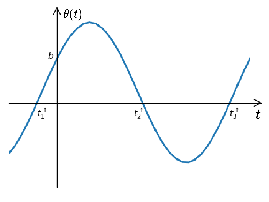
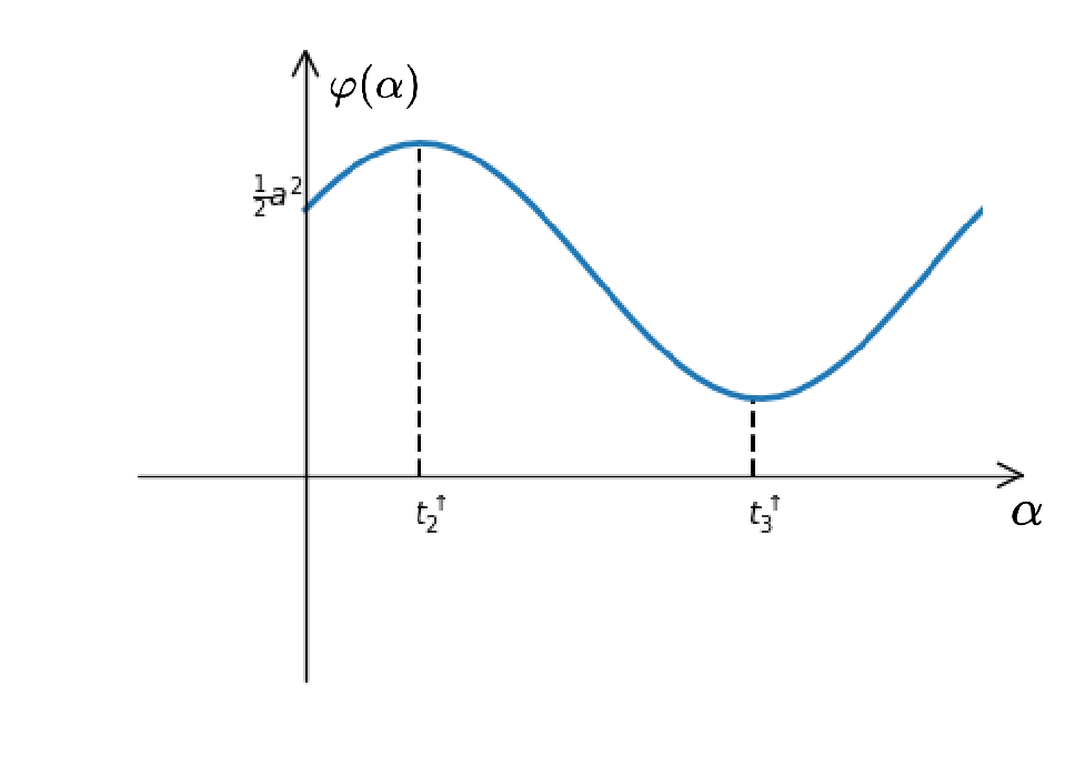
Figure 1: (a) $\theta\left(t\right)$ in Case 2.1. (b) $\varphi\left(\alpha\right)$ in Case 2.2.

The above discussions leads to the following proposition.

Proposition 2

Let $b\geq 0$. The solution of problem (18), denoted as $\alpha^{+}$, is given as follows.

1. $a\leq 0$, then $\alpha^{+}=0$;

2. $a>0$ and $b>\frac{4}{3\sqrt{3}}a^{\frac{3}{2}}$; then $\alpha^{+}$ = 0;

3. $a>0$ and $b\leq\frac{4}{3\sqrt{3}}a^{\frac{3}{2}}$. By the Cardano formula, one can compute $t_{1},t_{2},t_{3}$ by (19) and (20).

   Let $\alpha_{\max}=\max\{t_{1},t_{2},t_{3}\}$. Then $\alpha^{+}=\mathop{\arg}\min\limits_{\alpha\in\{0,\ \alpha_{\max}\}}\varphi(\alpha)$.

We summarize the algorithm for subproblem (18) as follows.

Algorithm 3 Algorithm for Subproblem (18)

S0.  Initialization a:=-$\frac{\hat{D}^{\zeta}_{ij}}{\rho},\;b=\frac{r}{\rho}W_{ij}.$

S1.  If $a\leq 0$ or $a>0$ and $b\leq\frac{4}{3\sqrt{3}}a^{\frac{3}{2}}$, let $\alpha^{+}=0$; else, go to S2.

S2.  Calculate $t_{1},t_{2},t_{3}$ by (19) and (20). Define $t_{\text{max}}:=\max\{t_{1},t_{2},t_{3}\}$. Let $\alpha^{+}=\mathop{\arg}\min\limits_{\alpha=\{0,\ t_{\max}\}}\varphi(\alpha)$

S3.  Output $\alpha^{+}$.

We end this section by the following remark.

Remark 5

From Algorithm 2 and Algorithm 3, one can see that we can obtain the explicit solution for subproblem (16). Consequently, although we deal with the matrix variable $D\in S^{2n}$ in EDM model (8), the computational cost is not high. The subproblem in Algorithm 1 can be calculated in an elementwise way with explicit formula as in Algorithm 2 and Algorithm 3. This again verifies the advantage of our EDM model (8) from the numerical computation point of view.

5 Numerical Results

In this section, we test our method (denoted as MP-EDM) on some datasets from UCI Machine Learning Repository. The experiments are conducted by using MATLAB (R2021b) on a Linux server of 256GB memory and 52 cores with Intel(R) Xeon(R) Gold 6230R 2.1GHz CPU. Our code can be found via https://www.researchgate.net/publication/376558182_release-MPEDM.

The parameters in MP-EDM is chosen as follows. For $w_{ij}$, a typical choice Sun is the following $k$-nearest neighbors defined by

$$\omega_{ij}=\left\{\begin{array}[]{lll}exp(-\varphi\|a_{i}-a_{j}\|^{2})&,&\ \text{ if }a_{i}\in k\mathrm{NN}\left(a_{j}\right)\text{ or }a_{j}\in k\mathrm{NN}\left(a_{i}\right),\\ 0,&&\ \text{otherwise.}\end{array}\right.$$ (21)

Here $k$NN$(x)$ is the set of $x$’s $k$-nearest neighbors, and $\varphi>0$ is a constant. We choose $\varphi=0.5$ in our experiments.

We stop MP-EDM when the following criterion QiXiuandZhou are satisfied

$$\text{Fprog}\leq\sqrt{n}\epsilon_{F}\text{ and Kprog}\leq\epsilon_{K},$$

where

$$\text{Fprog}=\frac{F_{\rho}(D^{\zeta-1})-F_{\rho}(D^{\zeta})}{1+F_{\rho}(D^{\zeta-1})},\ \text{Kprog}=1-\frac{\sum_{i=1}^{r}\left[\lambda_{i}^{2}-\left(\lambda_{i}-\lambda^{+}\right)^{2}\right]}{\sum_{i=1}^{n}\lambda_{i}^{2}}.$$

Here $\lambda_{1},\cdots,\lambda_{r}$ are the first $r$ largest eigenvalues of $D^{\top}$, and $\lambda_{i}^{+}=\max\{\lambda_{i},0\}$, $i\in[r]$. Fprog controls the convergence of $F_{\rho}(D^{\zeta})$ and Kprog measures the accuracy of eigenvalues. We set $\epsilon_{F}=5\times 10^{-3}$, $\epsilon_{K}=1\times 10^{-3}$.

The process of obtaining new labels. To obtain new labels from $D^{\zeta}$ by solving from model EDM($r$), first we obtain $\hat{y}_{1},\cdots,\hat{y}_{2n}$ by (3). Based on $\hat{y}_{n+1},\cdots,\hat{y}_{2n}$, we apply the multi-pass scheme as in ConvexClustering package of Sun to obtain the partition of $\{a_{1},\cdots,a_{n}\}$, denoted as $\hat{\mathcal{V}}=\{\hat{V}_{1},\cdots,\hat{V}_{\hat{K}}\}$, as presented in Algorithm 4, where $\hat{y}_{n+1},\cdots,\hat{y}_{2n}$ is the estimated centroid $x_{1},\cdots,x_{n}$. We choose $\epsilon_{d}=max\left(\log_{2}^{n},\ 10\right)\times\epsilon_{K}$ in Algorithm 4.

Algorithm 4 Algorithm for obtaining new labels

1:Centroids $\left[x_{1},\cdots,x_{n}\right]$, distance tolerance $\epsilon_{d}$

2:Initialize $\hat{\psi}:=\mathbf{0}\in\mathbb{R}^{n},\ N:=[n],\ \hat{K}:=1$.

3:for $N$ is not empty do

4:     Choose the first index $i\in N$, set $\hat{\psi}(a_{i})=\hat{K}$, remove $i$ from $N$.

5:     for $j\in N\setminus\{i\}$ do

6:         if $\|x_{i}-x_{j}\|\leq\epsilon_{d}$ then

7:              $\hat{\psi}(a_{j})=\hat{K}$, remove $j$ from $N$.

8:         end if

9:     end for

10:     $\hat{K}:=\hat{K}+1$

11:end for

12:Labels $\hat{\psi}$.

Measurement for clustering. We use Rand Index randindex (RI) and Normalized Mutual Information Infor (NMI) to measure whether the clustering is good or not. The bigger RI (NMI) is, the better. RI represents the ratio of pairs that are correctly clustered. Specifically, it is calculated by $\text{RI}=\frac{|S_{1}|+|S_{2}|}{\frac{n(n+1)}{2}}$, where $S_{1}$ is the set of pairs $a_{i},a_{j}$ such that $\psi(a_{i})=\psi(a_{j})$ and $\hat{\psi}(a_{i})=\hat{\psi}(a_{j})$, $S_{2}$ is the set of pairs $a_{i},a_{j}$ such that $\psi(a_{i})\neq\psi(a_{j})$ and $\hat{\psi}(a_{i})\neq\hat{\psi}(a_{j})$.

Let $\hat{n}_{i}=|\hat{V}_{i}|$. NMI is calculated by

$$\text{NMI}=\frac{\sum_{i=1}^{\hat{K}}\sum_{j=1}^{K}\left|\hat{V}_{i}\cap V_{j}\right|\log\left(\frac{n\left|\hat{V}_{i}\cap V_{j}\right|}{\hat{n}_{i}n_{j}}\right)}{\sqrt{\left(\sum_{i=1}^{\hat{K}}\hat{n}_{i}\log\left(\frac{\hat{n}_{i}}{n}\right)\right)\left(\sum_{j=1}^{K}n_{j}\log\left(\frac{n_{j}}{n}\right)\right)}}.$$

5.1 Performance of parameters in MP-EDM

In this part we test our algorithm with different combinations of parameters. Firstly we perform our algorithm on Wine, with $n=178,\ d=13,\ K=3$. To show how the parameters take effect on the clustering results, we set $r=13$, $k=50$, $\rho=100$, $\gamma=2$. Each time we only change one single parameter among $k$, $\gamma$ and $\rho$, and compare the RI and NMI, as shown in Figure 2. As one can see from Figure 2 (a), the choice of $k$ slightly affects the performance of clustering, and larger $k$ leads to higher RI and NMI. This is reasonable because large $k$ means that more neighbors are considered, which will lead to better clustering result. Figure 2 (b) and (c) imply that MP-EDM is not sensitive to the choice of $\rho$ and $\gamma$.

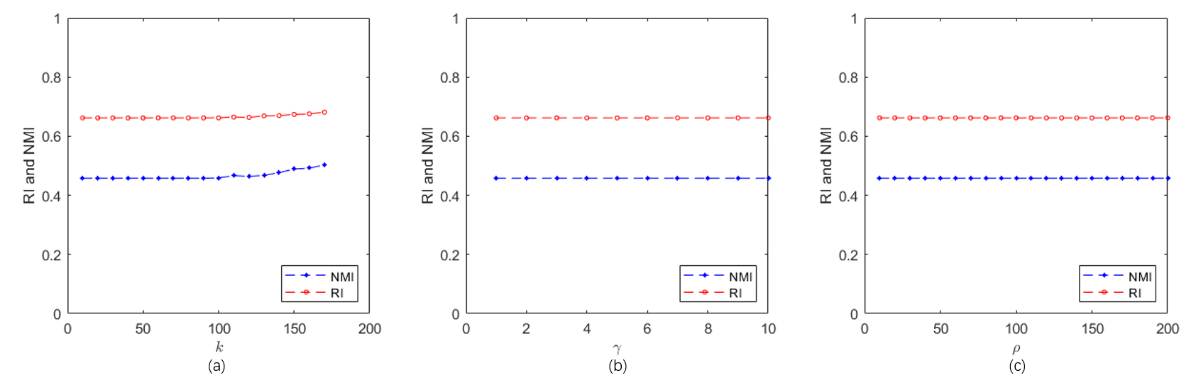
Figure 2: RI and NMI of different parameter combinations.

Secondly, we test the role of $r$ on Wine. We set $k=50,\ \rho=100,\ \gamma=2$, and change $r=1:1:13$. RI, NMI and the cputime are reported in Figure 3. It can be seen that for the case $r$ is much smaller than $d$, for example $r\leq 10$, the time consumed by MP-EDM is less than that of $r\geq 11$. This can be explained by more computational cost calculating $\Pi_{\mathcal{K}_{+}^{2n}(r)}(\cdot)$ by (14) and (15) for larger $r$. Moreover, the resulting RI and NMI is higher when $r\leq 5$, and they hardly change with $r\geq 5$. If we choose $r\ \textless\ d=13$, we can reduce the computational cost anf obtain good clustering results.

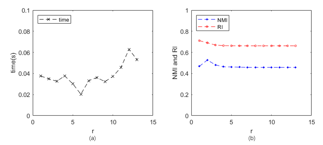
Figure 3: The cputime, RI and NMI of different $r$’s.

5.2 Comparison with other methods

Here we compare our algorithm with the popular K-Means, Spectral Clustering (SC), Hierarchical Clustering (HC) and semismooth Newton-CG augmented Lagrangian method (SSNAL) Sun2018 in ConvexClustering package on Iris, Wine, Letter-Recognition, Knowledge and MNIST. The results are reported in Table 1 - Table 3, where winners of RI and NMI are marked in bold.

From Table 1 one can see that MP-EDM gives competitive RI and NMI as SSNAL on Wine and Knowledge, and MP-EDM consumes less cputime than SSNAL. MP-EDM performs worse on Iris than other algorithms, but is much faster than SSNAL.

Data	Iris			Wine			Knowledge
($n,d,s,K$)	(150,4,4,3)			(178,13,13,3)			(400,5,5,4)
Methods	RI	NMI	Time(s)	RI	NMI	Time(s)	RI	NMI	Time(s)
MP-EDM	0.675	0.479	0.053	0.662	0.457	0.109	0.728	0.472	0.415
SSNAL	0.776	0.761	0.324	0.662	0.457	0.270	0.271	0.000	0.447
K-Means	0.873	0.741	0.003	0.691	0.424	0.027	0.669	0.230	0.004
SC	0.892	0.805	0.012	0.353	0.070	0.018	0.688	0.279	0.026
HC	0.776	0.735	0.001	0.362	0.091	0.005	0.278	0.039	0.004

Table 1: Clustering performance on Iris, Wine and Knowledge, $r=d$

For Letter-Recognition, we test MP-EDM on sizes of dataset with $n$ up to 10000. One can see from Table 2 that MP-EDM and SSNAL give very high RI and NMI on every $n$, but MP-EDM is faster than SSNAL. This can be explained by the fact that the two models SON($A,d$) and EDM($d$) are equivalent by Theorem 2. Although K-Means takes less time and yields a high RI, it performs poorly according to the measurement NMI.

	RI $|$ NMI $|$ Time
($n,s$)	(2000, 16)	(4000, 16)	(6000, 16)	(8000, 16)	(10000, 16)
MP-EDM	0.961 $|$ 0.668 $|$ 04	0.962 $|$ 0.649 $|$ 16	0.962 $|$ 0.641 $|$ 34	0.962 $|$ 0.635 $|$ 01:05	0.962 $|$ 0.632 $|$ 01:01
SSNAL	0.961 $|$ 0.657 $|$ 51	0.961 $|$ 0.632 $|$ 02:52	0.961 $|$ 0.620 $|$ 07:32	0.961 $|$ 0.612 $|$ 11:51	0.961 $|$ 0.606 $|$ 26:25
K-Means	0.927 $|$ 0.371 $|$ 0.04	0.929 $|$ 0.371 $|$ 0.07	0.930 $|$ 0.363 $|$ 0.09	0.931 $|$ 0.364 $|$ 0.12	0.931 $|$ 0.372 $|$ 0.20
SC	0.310 $|$ 0.299 $|$ 0.21	0.149 $|$ 0.186 $|$ 0.71	0.100 $|$ 0.135 $|$ 1.72	0.205 $|$ 0.207 $|$ 1.64	0.254 $|$ 0.264 $|$ 2.61
HC	0.927 $|$ 0.371 $|$ 0.04	0.927 $|$ 0.371 $|$ 0.17	0.927 $|$ 0.371 $|$ 0.34	0.927 $|$ 0.371 $|$ 0.68	0.927 $|$ 0.371 $|$ 1.10

Table 2: Clustering performance on Letter-Recognition with $d=16$, $K=26$.

In Table 3, we test $n=2000,4000,6000,8000$, with $d=784$, $K=10$. We also compare the performance of MP-EDM under $r=784$ and $r\ \textless\ 784$. We use MP-EDM-1, MP-EDM-2 and MP-EDM-3 to denote MP-EDM for $r=784$, $r=s$ and $r=100$ respectively. MP-EDM-1, MP-EDM-2 and MP-EDM-3 perform similar to SSNAL, in terms of RI and NMI. Moreover, MP-EDM-3 is much faster than MP-EDM-1 and MP-EDM-2 in terms of cputime.

	RI $|$ NMI $|$ Time
($n,s$)	(2000, 601)	(4000, 629)	(6000, 648)	(8000, 657)
MP-EDM-1	0.905 $|$ 0.537 $|$ 14:08	0.909 $|$ 0.559 $|$ 09:33	0.897 $|$ 0.523 $|$ 03:43	0.898 $|$ 0.511 $|$ 05:57
MP-EDM-2	0.905 $|$ 0.538 $|$ 30:24	0.910 $|$ 0.561 $|$ 08:32	0.896 $|$ 0.519 $|$ 05:02	0.898 $|$ 0.508 $|$ 09:42
MP-EDM-3	0.908 $|$ 0.574 $|$ 16	0.898 $|$ 0.519 $|$ 48	0.874 $|$ 0.465 $|$ 02:06	0.868 $|$ 0.439 $|$ 03:49
SSNAL	0.899 $|$ 0.549 $|$ 33:35	0.899 $|$ 0.526 $|$ 01:51:25	0.899 $|$ 0.514 $|$ 04:07:16	0.900 $|$ 0.506 $|$ 06:21:16
K-Means	0.885 $|$ 0.502 $|$ 0.23	0.888 $|$ 0.502 $|$ 0.31	0.892 $|$ 0.516 $|$ 0.49	0.878 $|$ 0.489 $|$ 0.52
SC	0.310 $|$ 0.299 $|$ 0.37	0.149 $|$ 0.186 $|$ 0.75	0.100 $|$ 0.135 $|$ 1.59	0.205 $|$ 0.207 $|$ 1.38
HC	0.074 $|$ 0.090 $|$ 0.14	0.059 $|$ 0.067 $|$ 0.32	0.051 $|$ 0.051 $|$ 0.73	0.061 $|$ 0.078 $|$ 0.81

Table 3: Clustering performance on MNIST with $d=784$ and $K=10$.

6 Conclusions

In this paper, we proposed a Euclidean distance matrix model based on the SON model for clustering. An efficient majorization penalty algorithm was proposed to solve the resulting model. The exact recovery property of the EDM model is established under some assumptions. Extensive Numerical experiments were conducted to demonstrate the efficiency of the proposed model and the majorization penalty algorithm. Notice that in Section 2, if $r<s$, $a_{1},\cdots,a_{n}$ can not be embedded into $r$-dimensional space. In this case, it is not clear whether the exact recovery property of EDM($r$) maintains or not. We will continue to investigate this question in future.

Appendix

Proof of Theorem 5 is presented in this part.

Proof

Recall $B$ defined in (7)

$$B:=\left\{D\in S^{2n}\;|\;diag(D)=0,\ D_{ij}=\|a_{i}-a_{j}\|^{2},\ i,j\in[n]\right\}.$$

Since $D_{\rho}^{*}$ is an optimal solution of (10), we have $D_{\rho}^{*}\in B$. Given $g\left(D\right)=0,\ f\left(D_{\rho}^{*}\right)\geq 0$,

$$f\left(D\right)=f\left(D\right)+\rho g\left(D\right)\geq f\left(D_{\rho}^{*}\right)+\rho g\left(D_{\rho}^{*}\right)\geq\rho g\left(D_{\rho}^{*}\right).$$

Therefore, we have

$$g\left(D_{\rho}^{*}\right)\leq\frac{f\left(D\right)}{\rho}\leq\frac{f\left(D\right)}{\rho_{\epsilon}}=\epsilon.$$

Since $g\left(D^{*}\right)=0,\ g\left(D_{\rho}^{*}\right)\geq 0$, we have

$$f\left(D^{*}\right)=f\left(D^{*}\right)+\rho g\left(D^{*}\right)\geq f\left(D_{\rho}^{*}\right)+\rho g\left(D_{\rho}^{*}\right)\geq f\left(D_{\rho}^{*}\right).\quad\qed$$

References

- (1) Bai, S.H., Qi, H.D.: Tackling the flip ambiguity in wireless sensor network localization and beyond. Digital Signal Processing 55(C), 85–97 (2016). DOI 10.1016/j.dsp.2016.05.006
- (2) Biswas, P., Liang, T.C., Toh, K.C., Ye, Y., Wang, T.C.: Semidefinite programming approaches for sensor network localization with noisy distance measurements. IEEE Transactions on Automation Science and Engineering 3(4), 360–371 (2006). DOI 10.1109/TASE.2006.877401
- (3) Borg, I., Groene, P.J.F.: Modern Multidimensional Scaling. Springer, Berlin (2005)
- (4) Chi, E.C., Lange, K.: Splitting methods for convex clustering. Journal of Computational and Graphical Statistics 24(4), 994–1013 (2015). DOI 10.1080/10618600.2014.948181
- (5) Cox, M.A.A., Cox, T.F.: Multidimensional Scaling. Springer Berlin Heidelberg, Berlin, Heidelberg (2008). DOI 10.1007/978-3-540-33037-0“˙14
- (6) Dattorro, J.: Convex Optimization and Euclidean Distance Geometry. Meboo Publishing, USA (2005)
- (7) Ding, C., Qi, H.D.: Convex optimization learning of faithful Euclidean distance representations in nonlinear dimensionality reduction. Mathematical Programming 164(1), 341–381 (2017). DOI 10.1007/s10107-016-1090-7
- (8) Fiedler, M.: Algebraic connectivity of graphs. Czechoslovak Mathematical Journal 23(2), 298–305 (1973)
- (9) Gao, Y.: Structured low rank matrix optimization problems: A penalty approach. Ph.D. thesis, National University of Singapore (2010)
- (10) Golub, G.H., Loan, C.V.: Matrix computations. Johns Hopkins University Press, Baltimore (1996)
- (11) Hocking, T.D., Joulin, A., Bach, F., Vert, J.P.: Clusterpath an algorithm for clustering using convex fusion penalties. 28th International Conference on Machine Learning pp. 341–381 (2011)
- (12) Hubert, L., Arabie, P.: Comparing partitions. Journal of Classification 2(1), 193–218 (1985). DOI 10.1007/BF01908075
- (13) Li, Q.N., Qi, H.D.: An inexact smoothing Newton method for Euclidean distance matrix optimization under ordinal constraints. Journal of Computational Mathematics 35(4), 469–485 (2017). DOI 10.4208/jcm.1702-m2016-0748
- (14) Li, Q.N., Qi, H.D., Xiu, N.H.: Block relaxation and majorization methods for the nearest correlation matrix with factor structure. Computational Optimization and Applications 50(2), 327–349 (2011). DOI 10.1007/s10589-010-9374-y
- (15) Lindsten, F., Ohlsson, H., Ljung, L.: Clustering using sum-of-norms regularization: With application to particle filter output computation. In: IEEE Statistical Signal Processing Workshop, pp. 201–204 (2011). DOI 10.1109/SSP.2011.5967659
- (16) Lu, S.T., Zhang, M., Li, Q.N.: Feasibility and a fast algorithm for Euclidean distance matrix optimization with ordinal constraints. Computational Optimization and Applications 76(2), 535–569 (2020). DOI 10.1007/s10589-020-00189-9
- (17) Pelckmans, K., Brabanter, J.D., Suykens, J., Moor, B.D.: Convex clustering shrinkage. In: PASCAL Workshop on Statistics and Optimization of Clustering Workshop (2005)
- (18) Qi, H.D.: A semismooth Newton’s method for the nearest Euclidean distance matrix problem. SIAM Journal on Matrix Analysis and Applications 34(34), 67–93 (2013). DOI 10.1137/110849523
- (19) Qi, H.D., Xiu, N.H., N, Yuan, X: A Lagrangian dual approach to the single source localization problem. IEEE Transactions on Signal Processing 61(15), 3815–3826 (2013). DOI 10.1109/TSP.2013.2264814
- (20) Qi, H.D., Yuan, X.M.: Computing the nearest Euclidean distance matrix with low embedding dimensions. Mathematical Programming 147(1-2), 351–389 (2014). DOI 10.1007/s10107-013-0726-0
- (21) Schoenberg, I.J.: Metric spaces and positive definite functions. Transactions of the American Mathematical Society 44(3), 522–536 (1938)
- (22) Sun, D.F., Toh, K.C., Yuan, Y.: Convex clustering: Model, theoretical guarantee and efficient algorithm. Journal of Machine Learning Research 22(9), 1–32 (2021). DOI 10.5555/3546258.3546267
- (23) Toh, K.C.: An inexact primal-dual path-following algorithm for convex quadratic SDP. Mathematical Programming 112(1), 221–254 (2008). DOI 10.1007/s10107-006-0088-y
- (24) Vinh, N.X., Epps, J., Bailey, J.: Information theoretic measures for clusterings comparison: Variants, properties, normalization and correction for chance. Journal of Machine Learning Research 11(95), 2837–2854 (2010). DOI 10.5555/1756006.1953024
- (25) Von Luxburg, U.: A tutorial on spectral clustering. Statistics and computing 17, 395–416 (2007). DOI 10.1007/s11222-007-9033-z
- (26) Wang, Z.W., Yuan, Y.C., Ma, J.M., Zeng, T.Y., Sun, D.F.: Randomly projected convex clustering model: Motivation, realization, and cluster recovery guarantees (2023). URL https://arxiv.org/abs/2303.16841
- (27) Yao, Z.Q., Dai, Y.J., Li, Q.N., Xie, D., Liu, Z.H.: A novel posture positioning method for multi-joint manipulators. IEEE Sensors Journal 20(23), 14310–14316 (2020). DOI 10.1109/JSEN.2020.3007701
- (28) Yuan, Y., Sun, D.F., Toh, K.C.: An efficient semismooth Newton based algorithm for convex clustering. In: 35th International Conference on Machine Learning, vol. 13, pp. 9085–9095 (2018)
- (29) Zhai, F.Z., Li, Q.N.: A Euclidean distance matrix model for protein molecular conformation. Journal of Global Optimization 76(4), 709–728 (2020). DOI 10.1007/s10898-019-00771-4
- (30) Zhou, S.L., Xiu, N.H., Qi, H.D.: A fast matrix majorization-projection method for constrained stress minimization in MDS. IEEE Transactions on Signal Processing 66(3), 4331–4346 (2018). DOI 10.1109/TSP.2018.2849734
- (31) Zhou, S.L., Xiu, N.H., Qi, H.D.: Robust Euclidean embedding via EDM optimization. Mathematical Programming Computation 12(3), 337–387 (2019). DOI 10.1109/TSP.2018.2849734