Fractal energy gaps and topological invariants in hBN/Graphene/hBN double moiré systems

Abstract

We calculate the electronic structure in quasiperiodic double-moiré systems of graphene sandwiched by hexagonal boron nitride, and identify the topological invariants of energy gaps. We find that the electronic spectrum contains a number of minigaps, and they exhibit a recursive fractal structure similar to the Hofstadter butterfly when plotted against the twist angle. Each of the energy gaps can be characterized by a set of integers, which are associated with an area in the momentum space. The corresponding area is geometrically interpreted as a quasi Brillouin zone, which is a polygon enclosed by multiple Bragg planes of the composite periods and can be uniquely specified by the plain wave projection in the weak potential limit.

I Introduction

In twisted multilayers of two-dimensional (2D) materials, the moiré inteference pattern causes the electronic band reconstruction leading to unusual physical properties highly tunable by the twist angle. The best known example is the twist bilayer grapheneLopes dos Santos et al. (2007); Mele (2010); Trambly de Laissardière et al. (2010); Shallcross et al. (2010); Morell et al. (2010); Bistritzer and MacDonald (2011); Moon and Koshino (2012); de Laissardiere et al. (2012), where the flat band formation at the magic angle gives rise to exotic phenomena Cao et al. (2018a, b); Yankowitz et al. (2019); Lu et al. (2019). The superlattice of graphene on hexagonal boron nitride (hBN) has also been extensively studied Dean et al. (2010); Kindermann et al. (2012); Wallbank et al. (2013); Mucha-Kruczyński et al. (2013); Jung et al. (2014); Moon and Koshino (2014); Dean et al. (2013); Ponomarenko et al. (2013); Hunt et al. (2013); Yu et al. (2014), where the moiré potential creates the superlattice subbands in the Dirac cone.

Recently, attention is also paid to systems where multiple moiré superperiods compete. The hBN/graphene/hBN stack Finney et al. (2019); Wang et al. (2019a, b); Yang et al. (2020); Andelkovic et al. (2020); Leconte and Jung (2020); Onodera et al. (2020); Kuiri et al. (2021) is a typical example, where the moiré pattern caused by graphene and upper hBN layer and that by graphene and lower hBN layer form an incommensurate doubly-periodic potential to graphene as shown in Fig. 1(a). A similar situation is also found in twisted bilayer graphene on hBN Shi et al. (2021); Shin et al. (2021); Huang et al. (2021) and in twisted trilayer graphene. Zhu et al. (2020); Lin et al. (2020); Park et al. (2021); Hao et al. (2021)

The hBN/graphene/hBN system is realized when a monolayer graphene is encapsulated by top and bottom hBN substrates. There the dual moiré effect is relevant only when the lattice orientations of upper and lower hBN layers are nearly aligned to graphene, since otherwise the moiré wavelength is too short and hardly affects the low-energy electronic states of graphene. Nearly-aligned hBN/graphene/hBN superlattices were experimentally fabricated using various techniques, Finney et al. (2019); Wang et al. (2019a, b); Yang et al. (2020); Onodera et al. (2020); Kuiri et al. (2021) and it was shown that the coexistence of the different super periods gives rise to multiple minigaps in the spectrum, which can never be seen in a single moiré potential.Wang et al. (2019a, b)

Figure 1: (a) Incommensurate moiré structure in trilayer system. (b) The atomic model of hBN/graphene/hBN trilayer system. Top and bottom hBN layers are stacked with twist angles $\theta^{\alpha}$ and $\theta^{\beta}$ from middle graphene layer. (c) Top and bottom moiré patterns. The moiré superlattice vector is depending on the twist angle, and the moiré angle $\phi$ increases as the twist angle increases.

Theoretically, double moiré systems are generally hard to treat because the two superlattice periods are incommensurate in general and then the Hamiltonian is essentially quasiperiodic. The band structure of the hBN/graphene/hBN system was calculated using large-scale numerical simulations Andelkovic et al. (2020); Leconte and Jung (2020), where several major gaps and pseudo gaps were found as traces in the energy spectrum against the twist angle.

Here we ask: How can we topologically characterize energy gaps in quasiperiodic systems? In a usual periodic system, the electronic spectrum is separated into the Bloch subbands accommodating equal electron density, and the number of the subbands below a given gap is a topological invariant. In a doubly-periodic system, however, the absence of the rigorous unit cell prevents the definition of the Brillouin zone, so the topological characterization is not obvious. In one-dimension (1D), an energy gap in a double peroid with wavenumbers $G^{\alpha}$ and $G^{\beta}$ is characterized by a pair of integers $p$ and $q$, where the electron density below the gap is given by $n_{e}=(pG^{\alpha}+qG^{\beta})/(2\pi)$. This is regarded the Bragg gap of the $(|p|+|q|)$th-order harmonics. The integers $p$ and $q$ are directly related to the the topological properties such as the adiabatic pumping Thouless (1983); Niu (1986); Kraus et al. (2012); Fujimoto et al. (2020) and also the quantum Hall effect.Thouless et al. (1982) In the hBN/graphene/hBN system, similarly, some of the gaps can be associated with the Bragg gap of a composite reciprocal lattice vector, $p\mathbf{G}_{1}^{\alpha}+q\mathbf{G}_{2}^{\alpha}+r\mathbf{G}_{1}^{\beta}+s\mathbf{G}_{2}^{\beta}$ where indeces $\alpha,\beta$ label the two different moiré patterns. Wang et al. (2019a, b); Andelkovic et al. (2020); Leconte and Jung (2020) This scheme successfully explains a few gaps in the low-energy region, while does not generally work for all the gaps in the spectrum.

In this paper, we calculate the electronic structure of the hBN/graphene/hBN system in changing the twist angle, and identify the topological numbers of all the energy gaps by using a different scheme. First, we compute the band structures for a series of the commensurate approximants to simulate a continuous change of the twist angle. We find that the electronic spectrum actually contains a number of minigaps, exhibiting a recursive fractal structure when plotted against the twist angle. The topological characterization for the energy gaps is employed as follows. Now the system has the four distinct reciprocal lattice vectors $\mathbf{G}_{1}^{\alpha},\mathbf{G}_{2}^{\alpha},\mathbf{G}_{1}^{\beta},\mathbf{G}_{2}^{\beta}$, and we can define a momentum-space area element $(\mathbf{G}_{i}^{\lambda}\times\mathbf{G}_{j}^{\mu})_{z}$ by combining two distinct vectors out of them. As a result, we have four linearly-independent areas $A_{1},\cdots,A_{4}$ as shown in Fig. 2(a), which can be viewed as projected areas of the four-dimensional hypercube. We find that each energy gap is characterized by a set of integers $m_{1},\cdots,m_{4}$ such that the electron density below the gap is given by $n_{e}=\sum_{i}m_{i}A_{i}/(2\pi)^{2}$. Moreover, we show that the area $\sum_{i}m_{i}A_{i}$ is geometrically interpreted as a quasi Brillouin zone, which is a certain polygon composed of multiple Bragg-plane segments as shown in Fig. 2(b). The quasi Brillouin zone for a given gap can be identified by the plain wave projection in the weak potential limit. The band-gap characterization proposed in this work would be useful in other quasi-periodic 2D systems, such as twisted trilayer graphene, twisted bilayer graphene on hBN above mentioned, and also 30^∘ twisted bilayer graphene. Ahn et al. (2018); Moon et al. (2019); Crosse and Moon (2021); Ha and Yang (2021)

The paper is organized as follows. In Sec. II, we define the commensurate approximants and introduce the effective continuum Hamiltonian for the hBN/graphene/hBN system. We calculate the energy spectrum in Sec. III.1, and specify the topological numbers of the band gaps in Sec. III.2. In Sec. III.3, we identify the quasi Brillouin zone associated with the topological numbers by using the plain wave projection. A brief conclusion is given in Sec. IV.

Figure 2: (a) Independent unit area elements $A_{1},A_{2},A_{3},A_{4}$ obtained by cross product of the reciprocal lattice vectors $\mathbf{G}_{1}^{\alpha},\mathbf{G}_{2}^{\alpha},\mathbf{G}_{1}^{\beta},\mathbf{G}_{2}^{\beta}$ in hBN/graphene/hBN double-moiré system [Eq. (41)]. The $A_{5}$ and $A_{6}$ (dashed areas) can be expressed by others as $A_{5}=-A_{3}-A_{4}$ and $A_{6}=A_{3}$. (b) Example of quasi Brillouin zone (thick lines), which is composed of the Bragg planes for composite reciprocal lattice vectors (thin lines). See, Fig. 9 for more details.

II Method

II.1 Atomic structure

We consider a hBN/graphene/hBN trilayer system as illustrated in Fig. 1, where the top ($\lambda=\alpha$) and bottom ($\lambda=\beta$) hBN layers are rotated by $\theta^{\alpha}$ and $\theta^{\beta}$, respectively, relative to the middle graphene layer. Graphene and hBN share the same honeycomb structure with different lattice constants, $a\approx 0.246\,\mathrm{nm}$ and $a_{\rm hBN}\approx 0.2504\,\mathrm{nm}$, respectively.Liu et al. (2003) We define $A$ and $B$ as sublattices for graphene, and $A^{\lambda}$ and $B^{\lambda}$ as nitrogen and boron sites of $\lambda$-th hBN layer, respectively. The geometry $\theta^{\lambda}=0$ is defined by the $AB$ bond and the $A^{\lambda}B^{\lambda}$ bond are parallel to each other.

The lattice vectors of graphene are given by $\mathbf{a}_{1}=a(1,0)$ and $\mathbf{a}_{2}=a(1/2,\sqrt{3}/2)$, and those of hBN layers of $\lambda=\alpha,\beta$ by

$$\mathbf{a}^{\lambda}_{i}=MR(\theta^{\lambda})\,\,\mathbf{a}_{i}\quad(i=1,2),$$ (1)

where $R(\theta^{\lambda})$ is the two-dimensional rotation matrix by $\theta^{\lambda}$, and $M=(1+\varepsilon)\mathbf{1}$ represents the isotropic expansion by the factor $1+\varepsilon=a_{\rm hBN}/a\approx 1.018$. In the following, we assume the twist angles $\theta^{\alpha}$ and $\theta^{\beta}$ are small enough (a few degree or less) such that the moiré super period is much greater than the atomic lattice constant $a$. The primitive lattice vectors of the moiré pattern of the layer $l$ are given by Moon and Koshino (2014); Koshino (2015)

$$\mathbf{L}_{i}^{\lambda}=[\mathbf{1}-R(\theta^{\lambda})^{-1}M^{-1}]^{-1}\mathbf{a}_{i}\quad(i=1,2).$$ (2)

The corresponding reciprocal lattice vectors are

$$\mathbf{G}_{i}^{\lambda}=[\mathbf{1}-M^{-1}R(\theta^{\lambda})]\mathbf{a}^{*}_{i}\quad(i=1,2),$$ (3)

where $\mathbf{a}^{*}_{i}$ is the reciprocal lattice vectors for graphene which satisfies $\mathbf{a}_{i}\cdot\mathbf{a}^{*}_{j}=2\pi\delta_{ij}$.

The moiré superlattice period is given by

$$|\mathbf{L}_{1}^{\lambda}|=|\mathbf{L}_{2}^{\lambda}|=\frac{1+\varepsilon}{\sqrt{\varepsilon^{2}+2(1+\varepsilon)(1-\cos\theta^{\lambda})}}\,a.$$ (4)

The moiré rotation angle, or the relative angle of $\mathbf{L}_{i}^{\lambda}$ to $\mathbf{a}_{i}$ is given by

$$\phi^{\lambda}={\rm arctan}\left(\frac{-\sin\theta^{\lambda}}{1+\varepsilon-\cos\theta^{\lambda}}\right).$$ (5)

Figure 3 plots (a) the moiré superlattice period $L$ and (b) the moiré rotation angle $\phi$ as a function of the twist angle $\theta$. The super period $L$ is $13.8\,\mathrm{nm}$ at $\theta=0^{\circ}$, and it decreases in increasing $\theta$. The rotation angle $\phi$ is zero at $\theta=0$ and rapidly increases in the negative direction in increasing $\theta$.

Figure 3: (a) Moiré period $L$ [Eq. (4)] and (b) the moiré rotation angle $\phi$ [Eq. (5)] as a function of the twist angle $\theta$

Figure 4: (a) Super moiré unit cell and (b) the corresponding reciprocal lattice of the commensurate approximant for $(\theta^{\alpha},\theta^{\beta})=(0,1.1908^{\circ})$, where $(n_{1}^{\alpha},n_{2}^{\alpha})=(1,1)$ and $(n_{1}^{\beta},n_{2}^{\beta})=(-1,3)$.

II.2 Commensurate moiré approximation

Generally, the two moiré superperiods of $\alpha$ and $\beta$ are incommensurate and hence there is no unit cell in the trilayer systems as a whole. In any $(\theta^{\alpha},\theta^{\beta})$, however, we always have a certain pair of lattice points of the two moiré patterns which happen to be very close to each other. The situation is expressed as

$$n_{1}^{\alpha}\bm{L}^{\alpha}_{1}+n_{2}^{\alpha}\bm{L}^{\alpha}_{2}=n_{1}^{\beta}\bm{L}^{\beta}_{1}+n_{2}^{\beta}\bm{L}^{\beta}_{2}+\Delta\mathbf{L},$$ (6)

where $n_{j}^{\lambda}$ are integers and $\Delta\mathbf{L}$ is the difference. When $\Delta\mathbf{L}$ is much smaller than the moiré periods, the electronic structure of such the system can be approximated by an exactly-commensurate system with $\Delta\mathbf{L}$ neglected. Specifically, it is obtained by slightly rotating and expanding / shrinking the moire patterns so that $\Delta\mathbf{L}$ vanishes. Figure 4(a) shows an actual example of commensurate approximant for $(\theta^{\alpha},\theta^{\beta})=(0,1.1908^{\circ})$, where $(n_{1}^{\alpha},n_{2}^{\alpha})=(1,1)$ and $(n_{1}^{\beta},n_{2}^{\beta})=(-1,3)$.

When $\Delta\mathbf{L}$ is neglected, Eq. (6) gives a primitive lattice vector of the commensurate super moiré structure, $\bm{L}^{\rm SM}_{1}$. The other primitive vector $\bm{L}^{\rm SM}_{2}$ is obtained by rotating $\bm{L}^{\rm SM}_{1}$ by 60^∘. As a result, we have

$$\left(\begin{array}[]{c}\bm{L}^{\rm SM}_{1}\\ \bm{L}^{\rm SM}_{2}\end{array}\right) = \left(\begin{array}[]{cc}n_{1}^{\alpha}&n_{2}^{\alpha}\\ -n_{2}^{\alpha}&n_{1}^{\alpha}+n_{2}^{\alpha}\end{array}\right)\left(\begin{array}[]{c}\bm{L}^{\alpha}_{1}\\ \bm{L}^{\alpha}_{2}\end{array}\right)$$ (13)

$$= \left(\begin{array}[]{cc}n_{1}^{\beta}&n_{2}^{\beta}\\ -n_{2}^{\beta}&n_{1}^{\beta}+n_{2}^{\beta}\end{array}\right)\left(\begin{array}[]{c}\bm{L}^{\beta}_{1}\\ \bm{L}^{\beta}_{2}\end{array}\right).$$ (18)

Correspondingly, the reciprocal superlattice vectors $\bm{G}^{\rm SM}_{1},\bm{G}^{\rm SM}_{2}$ are given by

$$\left(\begin{array}[]{c}\bm{G}^{\rm SM}_{1}\\ \bm{G}^{\rm SM}_{2}\end{array}\right) = \left[\left(\begin{array}[]{cc}n_{1}^{\alpha}&-n_{2}^{\alpha}\\ n_{2}^{\alpha}&n_{1}^{\alpha}+n_{2}^{\alpha}\end{array}\right)\right]^{-1}\left(\begin{array}[]{c}\bm{G}^{\alpha}_{1}\\ \bm{G}^{\alpha}_{2}\end{array}\right)$$ (25)

$$= \left[\left(\begin{array}[]{cc}n_{1}^{\beta}&-n_{2}^{\beta}\\ n_{2}^{\beta}&n_{1}^{\beta}+n_{2}^{\beta}\end{array}\right)\right]^{-1}\left(\begin{array}[]{c}\bm{G}^{\beta}_{1}\\ \bm{G}^{\beta}_{2}\end{array}\right).$$ (30)

Figure 4(b) is the reciprocal lattice corresponding to Fig. 4(a).

In the following, we consider two series of hBN/graphene/hBN trilayer systems,

$${\rm I:}\quad\,\,(\theta^{\alpha},\theta^{\beta})=(0,\theta); 0\leq\theta\leq 2\degree$$

$${\rm II:}\quad(\theta^{\alpha},\theta^{\beta})=(\theta,-\theta); 0\leq\theta\leq 2\degree$$ (31)

In each case, we find a set of $(\theta^{\alpha},\theta^{\beta})$ satisfying that $\Delta\mathbf{L}$ is less than 1% of $|n_{1}^{\alpha}\bm{L}^{\alpha}_{1}+n_{2}^{\alpha}\bm{L}^{\alpha}_{2}|$ and $n_{1}^{\alpha},n_{2}^{\alpha}\leq n_{\rm max}$, where $n_{\rm max}=12$ and 17 for series I and II, respectively. The full list of $(\theta^{\alpha},\theta^{\beta})$ in series I (II) is presented in Table 1 (2 and 3) in Appendix A. In series II, the list is dominated by exactly commensurate systems (i.e., $\Delta\mathbf{L}=0$) which appear when the moiré periods of $\alpha$ and $\beta$ are equal. For later reference, we label those commensuratel cases by $[(n_{1}^{\alpha},n_{2}^{\alpha}),(n_{1}^{\beta},n_{2}^{\beta})]$ as

$$p_{mn} \equiv[(m,n),\,(n,m)],$$

$$q_{mn} \equiv[(m,n),\,(m+n,-n)],$$

$$r_{mn} \equiv[(m,n),\,(m,-m-n)].$$ (32)

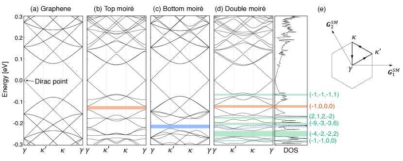
Figure 5: Band structure of $(\theta^{\alpha},\theta^{\beta})=(0\degree,1.1908\degree)$. The panel (d) shows the energy band of the full double moiré potential plotted along the symmetric line of the super moiré Brillouin zone shown in (e), with the corresponding DOS on the right. For comparison, we also show the energy bands with (a) no moiré potentials (intrinsic graphene), (b) only the top moiré potential and (c) only the bottom moiré potential, plotted on the same path. The first order gap of the top (bottom) moiré potential are colored by red (blue) and the double-moiré gaps by green. The dashed blue curve in (d) is the position of the first order gap of the bottom moiré potential, which actually does not open.

II.3 Effective Hamiltonian

Since the hBN has a semiconducting gap, the low-energy spectrum of the hBN/graphene/hBN system is dominated by the Dirac cones of graphene. We can derive the continuum Hamiltonian of the trilayer system in a similar manner to that for graphene-hBN bilayer. Kindermann et al. (2012); Wallbank et al. (2013); Mucha-Kruczyński et al. (2013); Jung et al. (2014); Moon and Koshino (2014); Dean et al. (2013); Ponomarenko et al. (2013); Hunt et al. (2013); Yu et al. (2014) It is written in $6\times 6$ matrix form as

$$H_{\rm eff}=\left(\begin{array}[]{ccc}H_{G}&U^{\alpha\dagger}&U^{\beta\dagger}\\ U^{\alpha}&H_{\rm hBN}&0\\ U^{\beta}&0&H_{\rm hBN}\\ \end{array}\right)$$ (33)

which works on the basis of $\{A,B,A^{\alpha},B^{\alpha},A^{\beta},B^{\beta}\}$. The $H_{\rm G}$ ($2\times 2$ matrix) is the Hamiltonian for graphene, which is given by

$$H_{\rm G}\approx-\hbar v{\mathbf{k}}\cdot\mbox{\boldmath$\sigma$}_{\xi},$$ (34)

where $\xi=\pm 1$ is the valley index graphene which correspond to the wave point $\mathbf{K}_{\xi}=-\xi(2\mathbf{a}^{*}_{1}+\mathbf{a}^{*}_{2})/3$, $\mathbf{k}$ is the relative wave number measured from $\mathbf{K}_{\xi}$ point, and $\mbox{\boldmath$\sigma$}_{\xi}=(\xi\sigma_{x},\sigma_{y})$ with Pauli matrices $\sigma_{x}$ and $\sigma_{y}$. The $H_{\rm hBN}$ in the second and third diagonal blocks is the Hamiltonian for monolayer hBN, Here we adopt an approximation only considering the on-site potential as Kindermann et al. (2012); Moon and Koshino (2014)

$$H_{\rm hBN}\approx\begin{pmatrix}V_{\rm N}&0\\ 0&V_{\rm B}\end{pmatrix}.$$ (35)

The off diagonal matrix $U^{\lambda}$ is the interlayer Hamiltonians of the twist angle $\theta^{\lambda}$, which is given by Moon and Koshino (2014)

$$U^{\lambda}=t_{0}\Biggl{[}\begin{pmatrix}1&1\\ 1&1\end{pmatrix}+\begin{pmatrix}1&\omega^{-\xi}\\ \omega^{\xi}&1\end{pmatrix}e^{i\xi\mathbf{G}^{\lambda}_{1}\cdot(\mathbf{r}-\mathbf{r}_{0}^{\lambda})}$$

$$\qquad\qquad+\begin{pmatrix}1&\omega^{\xi}\\ \omega^{-\xi}&1\end{pmatrix}e^{i\xi(\mathbf{G}^{\lambda}_{1}+\mathbf{G}^{\lambda}_{2})\cdot(\mathbf{r}-\mathbf{r}_{0}^{\lambda})}\Biggr{]},$$ (36)

where $t_{0}\approx 150\,\mathrm{meV}$ is the interlayer coupling energy, and $\mathbf{r}_{0}^{\lambda}$ is the origin of the moiré pattern of layer $\lambda$, which can be changed by sliding the hBN layer relative to graphene.Fujimoto et al. (2020)

The low-energy effective Hamiltonian for graphene can be obtained by eliminating the hBN bases by the second order perturbation. It is explicitly written as,

$$H_{\rm G}^{\rm(eff)} =H_{\rm G}+V_{\rm hBN}^{\alpha}+V_{\rm hBN}^{\beta},$$ (37)

where

$$V_{\rm hBN}^{\lambda} \equiv U^{\lambda\dagger}(-H_{\rm hBN})^{-1}U^{\lambda}$$ (38)

$$= V_{0}\begin{pmatrix}1&0\\ 0&1\end{pmatrix}+\Biggl{\{}V_{1}e^{i\xi\psi}\Biggl{[}\begin{pmatrix}1&\omega^{-\xi}\\ 1&\omega^{-\xi}\end{pmatrix}e^{i\xi\mathbf{G}^{\lambda}_{1}\cdot(\mathbf{r}-\mathbf{r}_{0}^{\lambda})}$$

$$+\begin{pmatrix}1&\omega^{\xi}\\ \omega^{\xi}&\omega^{-\xi}\end{pmatrix}e^{i\xi\mathbf{G}^{\lambda}_{2}\cdot(\mathbf{r}-\mathbf{r}_{0}^{\lambda})}+\begin{pmatrix}1&1\\ \omega^{-\xi}&\omega^{-\xi}\end{pmatrix}e^{i\xi\mathbf{G}^{\lambda}_{3}\cdot(\mathbf{r}-\mathbf{r}_{0}^{\lambda})}\Biggr{]}$$

$$\hskip 91.04881pt+{\rm h.c.}\Biggr{\}},$$

with

$$V_{0}=-3t_{0}^{2}\left(\frac{1}{V_{\rm N}}+\frac{1}{V_{\rm B}}\right),$$ (39)

$$V_{1}e^{i\psi}=-t_{0}^{2}\left(\frac{1}{V_{\rm N}}+\omega\frac{1}{V_{\rm B}}\right),$$ (40)

and $\mathbf{G}_{3}^{\lambda}=-\mathbf{G}_{1}^{\lambda}-\mathbf{G}_{2}^{\lambda}$, and $V_{0}\approx 29\,\mathrm{meV}$, $V_{1}\approx 21\,\mathrm{meV}$, and $\psi\approx-0.29$(rad). Moon and Koshino (2014)

Using the effective Hamiltonian of Eq. (33), we calculate the band structure of the approximate commensurate systems introduced in the previous section. The set of wavenumbers hybridized by the commensurate double moiré pattern is given by $\mathbf{q}_{m_{1},m_{2}}=\mathbf{k}+m_{1}\mathbf{G}_{1}^{\rm SM}+m_{2}\mathbf{G}_{2}^{\rm SM}$, where $m_{1}$ and $m_{2}$ are integers and $\mathbf{k}$ is a residual wavenumber defined inside the first super-moiré Brillouin zone spanned by $\mathbf{G}_{1}^{\rm SM}$ and $\mathbf{G}_{2}^{\rm SM}$. We construct the Hamiltonian matrix in the bases for graphene, $\{|\mathbf{q}_{m_{1},m_{2}},A\rangle,|\mathbf{q}_{m_{1},m_{2}},B\rangle\}$, with $k$-space cut-off $|\mathbf{q}_{m_{1},m_{2}}|<q_{c}$. Here we take $q_{c}=2|\mathbf{G}_{1}^{\beta}|$, which is about 0.54 eV for $\theta^{\beta}=0^{\circ}$ and 1.2 eV for $\theta^{\beta}=2^{\circ}$. Finally, the band diagram is obtained by plotting the eigenvalues of the Hamitonian matrix as a function of $\mathbf{k}$.

III Results

III.1 Electronic spectrum

As a typical example, we show the band structure of the commensurate approximant for $(\theta^{\alpha},\theta^{\beta})=(0,1.1908^{\circ})$, which was considered in Fig. 4. Here we set the origins of the moire potentials, $\mathbf{r}_{0}^{\alpha},\mathbf{r}_{0}^{\beta}$, to zero. Figure 5(d) shows the energy band plotted along the symmetric line of the super moiré Brillouin zone. For comparison, we also present the band structures (a) with no moiré potential (intrinsic graphene), (b) with only the top moiré potential and (c) with only the bottom moiré potential plotted on the same path. In all the panels, we set the origin of energy (vertical axis) at the Dirac point of graphene. In the single moiré systems in Fig. 5(b) and (c), the biggest gap in the valence band (red / blue regions) is the first order moiré gap corresponding to the electron density of one electron (per valley and per spin) for a moiré unit cell. In the double moiré system, on the other hand, we see a series of the higher order gaps (green) due to the coexistence of the different moiré periods.

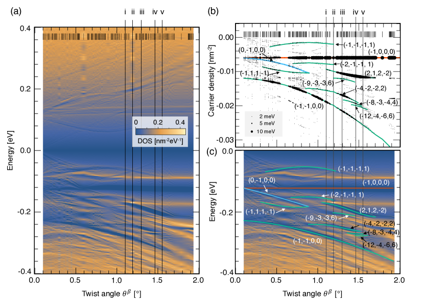
Figure 6: (a) Color map of the density of states (DOS) of the series I [$(\theta^{\alpha},\theta^{\beta})=(0,\theta^{\beta})$], plotted against $\theta^{\beta}$ and energy. The array of bars in the upper part of the figure represents $\theta^{\beta}$’s listed in Tables 1. (c) The lower part of (a), where the first-order gaps of the single moiré pattern $\lambda=\alpha$ and $\beta$ are highlighted by red and blue curves, respectively, and higher-order gaps are marked by green curves. (b) The corresponding map of the energy gaps with vertical axis converted to the electron density, where the size of the black dots represent the gap width.

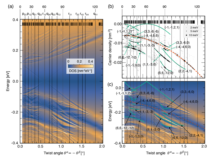
Figure 7: Plots similar to Fig. 6 for series II [$(\theta^{\alpha},\theta^{\beta})=(\theta,-\theta)$]. The vertical lines labeled by $p_{mn},q_{mn},r_{mn}$ represent the commensurate angles defined in Eq. (32), and the numbers on the top (0, 30, $\cdots$, 120) indicate the relative angle between the two moiré patterns, $\phi^{\beta}-\phi^{\alpha}$.

To study the twist-angle dependence of the electronic spectrum, we perform the band calculations for all the systems of the series I and II [Eq. (31)]. In commensurate systems, the band structure depends on the relative translation of the moire potentials, $\Delta\mathbf{r}_{0}=\mathbf{r}_{0}^{\alpha}-\mathbf{r}_{0}^{\beta}$. The dependence on $\Delta\mathbf{r}_{0}$ is generally greater in the systems of smaller $L_{\rm SM}$, and it quickly vanishes in increasing $L_{\rm SM}$. Here we average the DOS over 16 grid points of $\Delta\mathbf{r}_{0}$ for the systems with $L_{\rm SM}<50$ nm, and otherwise we just take $\Delta\mathbf{r}_{0}=0$, since the dependence is minor.

Figure 6(a) shows the color map of the density of states (DOS) calculated for the series I [$(\theta^{\alpha},\theta^{\beta})=(0,\theta^{\beta})$], plotted against $\theta^{\beta}$ and energy. Here the brighter color indicates larger DOS, and the dark blue represents the gap. The array of bars in the upper part of the figure represents $\theta^{\beta}$’s in the series I [listed in Tables 1]. The case $(\theta^{\alpha},\theta^{\beta})=(0,1.1908^{\circ})$ considered in Fig. 5 is marked by the label (ii). Figure 6(c) shows the lower part of (a), where the first-order gaps of the single moiré pattern $\lambda=\alpha$ and $\beta$ are highlighted by red and blue curves, respectively, and typical higher-order gaps are marked by green curves. Figure 6(b) is the corresponding map of the energy gaps with vertical axis converted to the electron density, where the size of the black dots represent the gap width. In these plots, we see that the spectrum continuously change as a function of the twist angle, even though the adjacent approximants in the series have completely different super moiré periods and thus different numbers of minibands.

Figure 7 shows similar plots for the series II plotted against $\theta^{\alpha}=-\theta^{\beta}$. The vertical lines labeled by $p_{mn},q_{mn},r_{mn}$ represent the commensurate angles defined in Eq. (32), and the numbers on the top (0, 30, $\cdots$, 120) indicate $\phi^{\beta}-\phi^{\alpha}$, or the relative angle between the two moiré patterns. The $r_{10}\,(\theta^{\alpha}\approx 0.5972\degree)$ and $q_{01}\,(\theta^{\alpha}\approx 1.8377\degree)$ are special cases where the relative angle of the two moiré patterns is 60^∘ and 120^∘, respectively, and hence the two moiré periods completely overlap. There we have a relatively small number of the subbands because of the coincidence of the double-period, but once moving away from these angles, we see that a number of tiny levels branching out just like Landau levels in a magnetic field. As a whole, we observe a recursive pattern ruled by the commensurate lines such as $p_{n,n\pm 1},q_{n,n\pm 1},r_{n,n\pm 1}$. The red dashed curve in Figs. 7 (b) and (c) indicate the positions of the first-order gaps of the two moiré patterns, which exactly match because of $|\theta^{\alpha}|=|\theta^{\beta}|$. We observe that the first-order gap closes throughout the figure (dashed line) only leaving a small-DOS region around. The reason for the absence of the first-order gap will be explained in the next section.

III.2 Topological invariants for band gaps

The microgap structure observed in Figs. 6 and 7 resembles the Hofstadter butterfly Hofstadter (1976), which is the energy spectrum of the two-dimensional periodic lattice in magnetic field. The Hofstadter system is essentially equivalent to the one-dimensional Hamiltonian with double period Harper (1955); Aubry and André (1980), where the fractal minigap structure emerges when the two periods are changed relatively to each other. There each minigap is characterized by a pair of integers $p$ and $q$, such that the electron density below the gap is given by $n_{e}=(pG^{\alpha}+qG^{\beta})/(2\pi)$ where $G^{\alpha}$ and $G^{\beta}$ are the wavenumbers for the two periods. The present hBN/graphene/hBN system is a two-dimensional version of this, where the double period is specified by $(\mathbf{G}_{1}^{\alpha},\mathbf{G}_{2}^{\alpha})$ and $(\mathbf{G}_{1}^{\beta},\mathbf{G}_{2}^{\beta})$. Actually, as shown in the following, all the gaps observed in Figs. 6 and 7 can be uniquely characterized by four topological integers associated with a specific $k$-space region.

Let us consider a general situation where the two moire patterns are incommensurate. We can define four independent unit-areas by combining the four independent reciprocal lattice vectors $\mathbf{G}_{1}^{\alpha},\mathbf{G}_{2}^{\alpha},\mathbf{G}_{1}^{\beta},\mathbf{G}_{2}^{\beta}$ as,

$$A_{1}=(\mathbf{G}_{1}^{\alpha}\times\mathbf{G}_{2}^{\alpha})_{z},\quad A_{2}=(\mathbf{G}_{1}^{\beta}\times\mathbf{G}_{2}^{\beta})_{z},$$

$$A_{3}=(\mathbf{G}_{1}^{\alpha}\times\mathbf{G}_{1}^{\beta})_{z},\quad A_{4}=(\mathbf{G}_{1}^{\alpha}\times\mathbf{G}_{2}^{\beta})_{z},$$ (41)

which are illustrated in Fig. 2(a). Here $(\cdots)_{z}$ represents the $z$-component perpendicular to the plane, and it can be negative depending on the relative angles between the two vectors. The $A_{1}$ and $A_{2}$ are the Brillouin-zone areas of the individual moiré patterns of $\lambda=\alpha$ and $\beta$, respectively, while $A_{3}$ and $A_{4}$ are cross terms which combine the reciprocal vectors of the different moiré patterns. We can also define two more unit areas

$$A_{5}=(\mathbf{G}_{2}^{\alpha}\times\mathbf{G}_{1}^{\beta})_{z},\quad A_{6}=(\mathbf{G}_{2}^{\alpha}\times\mathbf{G}_{2}^{\beta})_{z},$$ (42)

which are shown as dashed parallelgrams in Fig. 2. In hBN/grahpene/hBN system, however, they are not independent but can be expressed as $A_{5}=-A_{3}-A_{4}$ and $A_{6}=A_{3}$, considering that the angle between $\mathbf{G}_{1}^{\lambda}$ and $\mathbf{G}_{2}^{\lambda}$ is fixed to 120^∘. Therefore, a complete set of independent unit areas is given by $(A_{1},A_{2},A_{3},A_{4})$. The areas $A_{1},\cdots A_{6}$ can be regarded as the projection of faces of four-dimensional hypercube onto the physical 2D plane, which is analogous to the general argument of the quasicrystal. Walter and Deloudi (2009)

In a conventional periodic 2D system with primitive reciprocal lattice vectors $\mathbf{G}_{1}$ and $\mathbf{G}_{2}$, the electronic spectrum is separated into Bloch subbands, each of which accomodates the electron density $|\mathbf{G}_{1}\times\mathbf{G}_{2}|/(2\pi)^{2}$. In a doubly-periodic 2D system, in contrast, the areas $A_{1},\cdots,A_{4}$ all serve as units of the spectrum separation. More specifically, we find that the electron density (per spin and valley) from the Dirac point to any gap in the hBN/graphene/hBN system can be uniquely expressed with four integers $m_{1},m_{2},m_{3},m_{4}$ as

$$n_{e}=(m_{1}A_{1}+m_{2}A_{2}+m_{3}A_{3}+m_{4}A_{4})/(2\pi)^{2}.$$ (43)

These integers are topological invariants i.e., they never changes as long as the gap survives in a continuous change of the moire pattern.

Figure 6(c) shows $m_{1},m_{2},m_{3},m_{4}$ found for some major gaps in the case I. Figure 6(b) is the same plot but with the vertical axis being the electron density $n_{e}$, and the black dots represent spectral gaps with size indicating gap width. Here the integers $m_{1},\cdots,m_{4}$ are identified from the commensurate approximants as follows. In a commensurate case, $A_{1},A_{2},A_{3}$ and $A_{4}$ have the greatest common divisor $A_{\rm SM}=(\mathbf{G}_{1}^{\rm SM}\times\mathbf{G}_{2}^{\rm SM})_{z}$, so they can be written as $A_{i}=s_{i}A_{\rm SM}$ with integers $s_{i}\,(i=1,2,3,4)$. The $n_{e}$ is also quantized in units of $A_{\rm SM}/(2\pi)^{2}$, and each band gap is characterized by an integer $t=n_{e}/[A_{\rm SM}/(2\pi)^{2}]$, which is the number of occupied subbands measured from the Dirac point. Then Eq. (43) becomes the Diophantine equation $t=m_{1}s_{1}+m_{2}s_{2}+m_{3}s_{3}+m_{4}s_{4}$. For each gap in Fig. 6(c), we have the Diophantine equations as many as the number of the data points (i.e., the different systems), and the $(m_{1},m_{2},m_{3},m_{4})$ is obtained as a unique solution of the set of equations. Here note that the area $m_{1}A_{1}+m_{2}A_{2}+m_{3}A_{3}+m_{4}A_{4}$ is a continuous function of the twist angle, while $A_{\rm SM}$ (and thus $t,s_{i}$) can only be defined for commensurate systems and it discontinuously changes in changing the twist angle. This result indicates that the same $(m_{1},m_{2},m_{3},m_{4})$ are shared by infinitely many commensurate approximants (with $A_{\rm SM}$ ranging from 0 to infinity) which exist in a close vicinity of a specific $(\theta^{\alpha},\theta^{\beta})$, and hence it is valid in the limit of $A_{\rm SM}\to\infty$, i.e., incommensurate systems.

Figures 7 (b) and (c) are similar plots for the case II. Here the condition $|\theta^{\alpha}|=|\theta^{\beta}|$ forces $A_{1}=A_{2}$, and then $m_{1}$ and $m_{2}$ becomes indeterminate. We can resolve the two integers by considering an infinitesimal rotation of either top or bottom hBN layer, and it turns out that $m_{1}=m_{2}$ for any gaps of the case II. This is explicitly proved as follows. By starting from a case-II system $(\theta^{\alpha},\theta^{\beta})=(\theta,-\theta)$, we can consider two distinct systems $X:(\theta^{\alpha},\theta^{\beta})=(\theta+\delta\theta,-\theta)$ and $X^{\prime}:(\theta^{\alpha},\theta^{\beta})=(\theta,-\theta-\delta\theta)$. The system $X$ and $X^{\prime}$ are actually identical by turning the whole system by 180^∘ with respect to an in-plane axis, and hence they have the exactly the same energy spectrum. The same energy gap is labeled by a different set of integers as $m_{i}$ and $m^{\prime}_{i}$ for $X$ and $X^{\prime}$, respectively, which satisfy $\sum_{i}m_{i}A_{i}=\sum_{i}m^{\prime}_{i}A^{\prime}_{i}$. By considering the layer $\lambda=\alpha,\beta$ are interchanged in the 180^∘-rotation process, the unit areas of $X$ and $X^{\prime}$ are related by $(A_{1},A_{2},A_{3},A_{4})=(A^{\prime}_{2},A^{\prime}_{1},A^{\prime}_{3},A^{\prime}_{4})$, and this leads to the condition $(m_{1},m_{2},m_{3},m_{4})=(m^{\prime}_{2},m^{\prime}_{1},m^{\prime}_{3},m^{\prime}_{4})$. When the gap survives in the limit of $\delta\theta\to 0$, we have $m_{i}=m^{\prime}_{i}$, and hence we conclude $m_{1}=m_{2}$. The constraint $m_{1}=m_{2}$ explains why the first-order gap of individual moiré potential, $(\pm 1,0,0,0)$ and $(0,\pm 1,0,0)$ cannot open in Fig. 7(b).

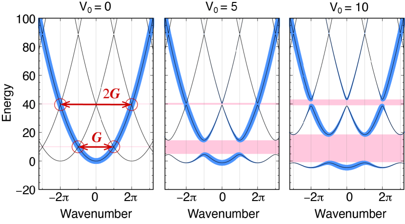
Figure 8: Band structure of a 1D Hamiltonian $H=-\partial^{2}/\partial x^{2}+2V_{0}\cos Gx$ with $V_{0}=0,5,10$. The black solid lines represent the band dispersion $\varepsilon_{nk}$ in the extended zone scheme, and the size of blue points represents the spectral weight projected to the plain wave, $A(q,\varepsilon)$.

The constraint among the six unit areas $A_{1},\cdots,A_{6}$ can be broken by uniformly distorting either top or bottom hBN layer such that 120^∘ symmetry is broken. If we extend the parameter space to such the distorted systems, we should need six topological integers $(m_{1},\cdots m_{6})$ to characterize minigaps, where the electron density is given by $\sum_{i=1}^{6}m_{i}A_{i}$. This is similar to situation in the series II, where $m_{1}$ and $m_{2}$ can be resolved by breaking the condition $A_{1}=A_{2}$.

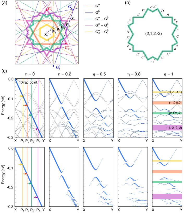
Figure 9: (a) Quasi Brillouin zones of $(\theta^{\alpha},\theta^{\beta})=(0\degree,1.1908\degree)$, where thick lines with different colors correspond to the four gaps indicated in (c). Thin lines are the Bragg planes corresponding to different reciprocal lattice vectors. For instance, the red lines are the perpendicular bisector of $\mathbf{G}_{1}^{\alpha}$ and its $60n^{\circ}$ rotation. (b) Quasi Brillouin zone of the gap $(2,1,2,-2)$, where $x$ and $x^{\prime}$ represents a pair of boundary segments connected by the moiré potential. (c) Band structure on a path from $X$ to $Y$ shown in (a) calculated for $(0\degree,1.1908\degree)$ with the moiré potentials reduced by the factor $\eta\,(0\leq\eta\leq 1)$. The black solid lines represent the band dispersion plotted in the extended zone scheme, and the blue dots represent the spectral weight $A(\mathbf{q},\varepsilon)$. The bottom panels show the same plot without the band lines.

III.3 Quasi Brillouin zones

Actually, the area $m_{1}A_{1}+m_{2}A_{2}+m_{3}A_{3}+m_{4}A_{4}$ can be associated with a specific region in the momentum space, which is referred to as quasi Brillouin zone. In a conventional periodic 2D system defined by $\mathbf{G}_{1}$ and $\mathbf{G}_{2}$, the Brillouin zones $(n=1,2,3\cdots)$ are defined by a series of certain regions bounded by the Bragg planes, i.e., the perpendicular bisectors of the reciprocal vectors $n_{1}\mathbf{G}_{1}+n_{2}\mathbf{G}_{2}$. Ashcroft et al. (1976) There all the Brillouin zones have equal area of $|\mathbf{G}_{1}\times\mathbf{G}_{2}|$, and therefore the carrier density below any gap is quantized to an integer multiple of the area. In a doubly-periodic 2D system, similarly, we can define a quasi Brillouin zone as an area bound by the Bragg planes for composite reciprocal vectors $p\mathbf{G}_{1}^{\alpha}+q\mathbf{G}_{2}^{\alpha}+r\mathbf{G}_{1}^{\beta}+s\mathbf{G}_{2}^{\beta}$. In conventional 3D quasicrystals such as Al-Mn alloys, the idea of the quasi Brillouin zones was used to explain the pseudogaps and the stability of the system. Smith and Ashcroft (1987) In an incommensurate case, generally, the momentum space is filled by infinitely many Bragg planes, and there is no systematic way to define quasi Brillouin zones as in the periodic case. But here, we claim that each single gap in the spectrum can be associated with a specific figure, and the area is equal to $m_{1}A_{1}+m_{2}A_{2}+m_{3}A_{3}+m_{4}A_{4}$. Such figures include a simple hexagon defined by a single reciprocal vector as considered in the previous works Wang et al. (2019b); Andelkovic et al. (2020); Leconte and Jung (2020), but more generally, it can be a non-convex polygon composed of multiple segments of different Bragg planes as shown in Fig. 9(a).

The shape of the quasi Brillouin zone for a given gap can be specified by the plain wave projection with the zero potential limit as follows. Let us explain the scheme using a simple one-dimensional Hamiltonian with a single periodic potential, $H=-\partial^{2}/\partial x^{2}+2V_{0}\cos Gx$, where $G=2\pi$. The eigenenergy and the eigenfunctions are labeled as $\varepsilon_{nk}$ and $|\psi_{nk}\rangle$, respectively, where $n$ is the band index and $k$ is the Bloch wavenumber in the first Brillouin zone $(-\pi\leq k\leq\pi)$. Figure 8 shows the band structures calculated for different potential amplitudes, $V_{0}=0,5,10$. The black solid lines represent the band dispersion $\varepsilon_{nk}$ plotted in the extended zone scheme, and the size of overlapped blue points represents the spectral weight projected to the plain wave, or

$$A(q,\varepsilon)=\sum_{n,k}|\langle q|\psi_{nk}\rangle|^{2}\delta(\varepsilon-\varepsilon_{nk}),$$ (44)

where $|q\rangle=e^{iqx}$ is the plain wave with $-\infty<q<\infty$, and the summation in $k$ is taken over the first Brillouin zone. The pink regions indicate the first and the second energy gaps. In decreasing the potential amplitude $V_{0}$, the gaps are narrowing, and the spectral weight approaches a simple parabola $\varepsilon=q^{2}$. In the limit of $V_{0}\to 0$, we can specify the points on the parabola, at which the energy gap opens in an infinitesimal $V_{0}$ (marked by red circles). These points actually determines the Brillouin zone boundary.

The same strategy works for the double-period system as well. In our hBN/graphene/hBN system, we define the spectral weight as

$$A(\mathbf{q},\varepsilon)=\sum_{\alpha}\sum_{X}|\langle\mathbf{q},X|\psi_{\alpha}\rangle|^{2}\delta(\varepsilon-\varepsilon_{\alpha}),$$ (45)

where $\varepsilon_{\alpha}$ and $|\psi_{\alpha}\rangle$ are the eigenenergy and the eigenstates of the system, and $|\mathbf{q},X\rangle$ is the plain wave basis of the sublattice $X=A,B$ of the monolayer graphene. For example, we take the commensurate approximant for $(\theta^{\alpha},\theta^{\beta})=(0\degree,1.1908\degree)$ considered in Figs. 4 and 5, and calculate the eigenstates of the Hamiltonian Eq. (33) with the moiré potentials $(V_{\rm hBN}^{\alpha},V_{\rm hBN}^{\beta})$ reduced by the factor $\eta\,(0\leq\eta\leq 1)$. Figure 9(c) shows the band structures from $\eta=0$ to 1, calculated on a path from $X$ (graphene’s Dirac point) to a certain point $Y$ shown in Fig. 9(a). The black solid lines represent the band dispersion plotted in the extended zone scheme, and the blue dots represent the spectral weight $A(\mathbf{q},\varepsilon)$. At $\eta=0$, we just have the graphene’s Dirac cone. By tracing the gaps in the spectral weight in decreasing $\eta$ from 1 to 0, we can specify the gap opening points just as in the one-dimensional case.

In Fig. 9(c), we consider four gaps with different indeces of $(m_{1},...,m_{4})$. The $(-1,0,0,0)$ is the first-order gap of the moiré potential $\lambda=\alpha$, and others are double-moire gaps caused by the coexistence of the two moiré patterns. In the limit $\eta\to 0$, we find the gap-opening wave numbers $P_{1},\cdots,P_{4}$ for these gaps. By following the same procedure for paths in different directions, we finally obtain the quasi Brillouin zone on the $(k_{x},k_{y})$ plane as the traces of $P_{1},\cdots,P_{4}$, which are illustrated as thick colored lines in Fig. 9(a). The figures are composed of segments of the Bragg planes, which are shown as thin lines. The first-order gap $(-1,0,0,0)$ gives a regular hexagon, which is the first Brillouin zone of the moiré potential of $\lambda=\alpha$. The double-moire gap $(-1,-1,-1,1)$ also gives a hexagon but with a smaller size, which corresponds to the first Brillioin zone of a small reciprocal lattice vectors $\mathbf{G}_{2}^{\alpha}+\mathbf{G}_{1}^{\beta}$. In contrast, the gaps $(2,1,2,-2)$ and $(-4,-2,-2,-2)$ are associated with flower-like complex figures composed of multiple Bragg line segments. In any cases, the area of the figure is shown to be exactly equal to $m_{1}A_{1}+m_{2}A_{2}+m_{3}A_{3}+m_{4}A_{4}$. Just as the conventional Brillouin zone in a periodic system, the quasi Brillouin zone is also a closed object, in that any sides of the boundary are precisely sticked to the other side and one can never go out of the region by crossing the boundary.

The quasi Brillouin zone continuously changes in changing the twist angle, regardless of the unit cell size of the commensurate approximants. Figure 10 shows the same plot calculated for a slightly different angle $(\theta^{\alpha},\theta^{\beta})=(0,1.2967^{\circ})$ [(iii) in Fig. 6]. The super moiré unit area of the system is about 10 times greater than that of Fig. 9(c), and accordingly we see much more band lines due to the band folding into the smaller Brillouin zone. If we see the spectral weight (blue dots), however, we find that it exhibits a similar structure to Fig. 9(c) (except that the gap $(-1,-1,-1,1)$ is not fully open), and the gaps close at the Bragg planes with the same indeces in the limit of $\eta\to 0$. As a result, we end up with nearly the same shape of the quasi Brilluoin zone as shown in Fig. 11(iii). In Fig. 10, we see a number of extra band lines are just overlapping but hardly contribute to the spectral weight, and therefore they are neglected in the identification of the zone boundary. Because of this, the quasi Brillouin zone obtained here is generally different from one obtained by sorting all the eigenvalues in energy and tracking the same level index in the limit of the zero potential Gambaudo and Vignolo (2014), which is fully affected by all the overlapping band lines.

In Fig. 11, we show the continuous evolution of the quasi Brillouin zones as a function of the twist angle from (i) to (v) [corresponding to the labels in Fig. 6], where the figure continuously changes regardless of the discontinuous change of the rigorous period of the approximants. The areas of the figures are always equal to $m_{1}A_{1}+m_{2}A_{2}+m_{3}A_{3}+m_{4}A_{4}$.

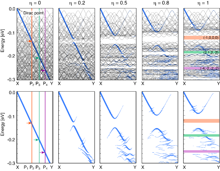
Figure 10: Plot similar to Fig. 9(c) calculated for $(\theta^{\alpha},\theta^{\beta})=(0\degree,1.2967\degree)$.

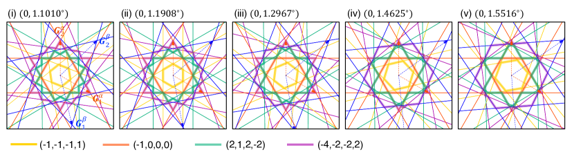
Figure 11: Quasi Brilluoin zones similar to Fig. 9(a) calculated for five different angles. The indeces (i) to (v) correspond to the labels in Fig. 6.

IV Conclusion

We theoretically studied the electronic structure of the hBN/graphene/hBN double-moiré system as a function of the top and bottom twist angles, and demonstrated that the spectrum consists of a number of fractal minigaps characterized by the non-trivial topological numbers. Specifically, each energy gap is characterized by a set of integers $(m_{1},\cdots,m_{4})$, where the electron density below the gap is given by $n_{e}=\sum_{i}m_{i}A_{i}/(2\pi)^{2}$ with characteristic momentum-space areas $A_{1},\cdots,A_{4}$. The area $\sum_{i}m_{i}A_{i}$ corresponds to a quasi Brillouin zone bounded by multiple Bragg planes, which can be uniquely identified by the spectral distribution in the zero potential limit. In changing the twist angles, the quasi Brillouin zone also changes continuously regardless of the commensurability of the double moiré pattern.

We neglect the lattice relaxation effect throughout this work for simplicity, while the general theoretical scheme to characterize the band gap is valid as long as the system has a well-defined double period. The topological band-gap characterization proposed in this work should also be useful in other quasi-periodic 2D systems, such as twisted trilayer graphene Zhu et al. (2020); Lin et al. (2020); Park et al. (2021); Hao et al. (2021), twisted bilayer graphene on hBN Shi et al. (2021); Shin et al. (2021); Huang et al. (2021) , and also 30^∘ twisted bilayer graphene. Ahn et al. (2018); Moon et al. (2019); Crosse and Moon (2021); Ha and Yang (2021)

V Acknowledgments

This work was supported in part by JSPS KAKENHI Grant Number JP20H01840 and JP20H00127 and by JST CREST Grant Number JPMJCR20T3, Japan.

Appendix A List of commensurate approximants

We present the list of approximate commensurate systems of series I in Table 1, and those of series II in Table 2 and 3. The tables show the twist angle, a set of integers $(n_{1}^{\alpha},n_{2}^{\alpha},n_{1}^{\beta},n_{2}^{\beta})$, the super moiré period $L^{\rm SM}$[nm], and the correction $\Delta L$[nm] from the original incommensurate structure.

Table 1: List of approximate commensurate systems of of series (I)$(\theta^{\alpha},\theta^{\beta})=(0,\theta)$. The $L^{\rm SM}$[nm] is the super moiré period, and $\Delta L$[nm] is the correction from the original incommensurate structure (see the text).

$\theta$ [°]	$n_{1}^{\alpha}$	$n_{2}^{\alpha}$	$n_{1}^{\beta}$	$n_{2}^{\beta}$	$L^{\rm SM}$	$\Delta L$	$\theta$ [°]	$n_{1}^{\alpha}$	$n_{2}^{\alpha}$	$n_{1}^{\beta}$	$n_{2}^{\beta}$	$L^{\rm SM}$	$\Delta L$	$\theta$ [°]	$n_{1}^{\alpha}$	$n_{2}^{\alpha}$	$n_{1}^{\beta}$	$n_{2}^{\beta}$	$L^{\rm SM}$	$\Delta L$
0.0992	6	6	5	7	144.64	0.0120	0.6985	11	1	6	10	160.51	0.4494	1.2967	5	1	0	9	77.49	0.0913
0.1083	11	11	9	13	265.18	0.0262	0.7009	11	6	2	17	207.84	0.3282	1.3109	8	7	-8	24	180.94	0.3575
0.1191	5	5	4	6	120.54	0.0144	0.7145	5	0	3	4	69.59	0.2464	1.3152	9	1	1	15	132.77	0.2972
0.1323	9	9	7	11	216.97	0.0319	0.7320	4	9	-5	16	160.51	0.1011	1.3238	3	10	-14	22	164.09	0.0440
0.1489	4	4	3	5	96.43	0.0179	0.7372	12	5	3	17	210.62	0.3335	1.3296	7	10	-13	28	205.97	0.1582
0.1624	11	0	10	2	153.10	0.0337	0.7443	4	4	-1	9	96.43	0.3654	1.3477	6	9	-12	25	182.01	0.2393
0.1701	7	7	5	9	168.75	0.0408	0.7513	7	12	-6	23	231.65	0.1193	1.3480	10	9	-11	31	229.12	0.3407
0.1786	10	0	9	2	139.18	0.0370	0.7550	11	4	3	15	187.25	0.3104	1.3526	10	5	-5	24	184.12	0.1326
0.1985	3	3	2	4	72.32	0.0237	0.7655	7	0	4	6	97.43	0.3867	1.3599	10	1	1	17	146.64	0.1881
0.2137	11	3	9	6	177.70	0.4663	0.7775	3	10	-7	17	164.09	0.1983	1.3666	9	8	-10	28	205.03	0.2428
0.2165	11	11	7	15	265.18	0.1029	0.7822	9	7	-1	18	193.36	0.3986	1.3831	2	10	-15	21	154.99	0.0052
0.2233	8	0	7	2	111.35	0.0459	0.7852	12	10	-2	25	265.54	0.0584	1.3900	8	7	-9	25	180.94	0.1668
0.2382	5	5	3	7	120.54	0.0563	0.7939	3	3	-1	7	72.32	0.3046	1.4086	2	6	-9	14	100.37	0.1440
0.2457	12	5	9	9	210.62	0.3425	0.8042	11	9	-2	23	241.47	0.0927	1.4207	7	6	-8	22	156.85	0.1219
0.2481	12	12	7	17	289.29	0.1464	0.8087	8	6	-1	16	169.32	0.1624	1.4356	4	8	-12	21	147.30	0.0359
0.2552	7	0	6	2	97.43	0.0521	0.8203	5	3	0	9	97.43	0.3427	1.4492	6	10	-15	28	194.86	0.2768
0.2646	9	9	5	13	216.97	0.1245	0.8273	10	8	-2	21	217.41	0.2860	1.4571	10	8	-11	31	217.41	0.3157
0.2707	11	11	6	16	265.18	0.1589	0.8344	12	8	-1	23	242.67	0.1292	1.4625	6	5	-7	19	132.77	0.1229
0.2977	2	2	1	3	48.21	0.0347	0.8440	7	5	-1	14	145.31	0.1614	1.4716	10	3	-3	22	164.09	0.0317
0.3248	11	0	9	4	153.10	0.1302	0.8518	9	5	0	16	171.03	0.0635	1.4904	9	7	-10	28	193.36	0.2114
0.3308	9	9	4	14	216.97	0.1911	0.8577	11	5	1	18	197.33	0.1873	1.5103	3	8	-13	20	137.08	0.1014
0.3402	7	7	3	11	168.75	0.1568	0.8606	11	7	-1	21	218.74	0.3712	1.5228	5	4	-6	16	108.71	0.1957
0.3450	12	7	7	13	231.65	0.1751	0.8931	2	0	1	2	27.84	0.1415	1.5330	8	6	-9	25	169.32	0.0362
0.3573	5	0	4	2	69.59	0.0709	0.9287	5	11	-9	22	197.33	0.0240	1.5516	3	2	-3	9	60.67	0.1985
0.3721	8	8	3	13	192.86	0.2124	0.9346	5	9	-7	19	171.03	0.0970	1.5689	4	10	-17	26	173.84	0.1515
0.3789	11	11	4	18	265.18	0.3021	0.9423	5	7	-5	16	145.31	0.3127	1.5785	1	8	-14	17	118.92	0.0345
0.3970	3	3	1	5	72.32	0.0899	0.9498	3	7	-6	14	123.71	0.4554	1.5898	7	5	-8	22	145.31	0.2386
0.4168	10	10	3	17	241.07	0.3281	0.9519	8	12	-9	27	242.67	0.1934	1.5999	1	9	-16	19	132.77	0.3700
0.4253	7	7	2	12	168.75	0.2385	0.9662	3	5	-4	11	97.43	0.1633	1.6065	8	5	-8	24	158.08	0.1204
0.4303	11	7	5	14	218.74	0.0922	0.9777	6	8	-6	19	169.32	0.1629	1.6173	4	3	-5	13	84.66	0.3899
0.4466	4	0	3	2	55.67	0.0861	0.9829	12	5	0	21	210.62	0.0849	1.6210	9	5	-8	26	171.03	0.3885
0.4631	9	9	2	16	216.97	0.3587	0.9923	3	3	-2	8	72.32	0.4324	1.6281	2	10	-18	23	154.99	0.1456
0.4673	5	9	-1	14	171.03	0.2277	1.0043	7	9	-7	22	193.36	0.1051	1.6406	5	3	-5	15	97.43	0.1220
0.4763	5	5	1	9	120.54	0.2098	1.0108	4	6	-5	14	121.34	0.3894	1.6590	6	3	-5	17	110.47	0.0304
0.4872	11	0	8	6	153.10	0.2776	1.0250	8	10	-8	25	217.41	0.1063	1.6735	7	3	-5	19	123.71	0.1045
0.4962	6	6	1	11	144.64	0.2711	1.0314	8	3	0	14	137.08	0.1263	1.6853	8	3	-5	21	137.08	0.1239
0.5104	7	0	5	4	97.43	0.1921	1.0524	1	8	-9	14	118.92	0.3587	1.6950	9	3	-5	23	150.55	0.1037
0.5210	8	8	1	15	192.86	0.3947	1.0909	8	10	-9	26	217.41	0.3308	1.7030	10	3	-5	25	164.09	0.0541
0.5262	1	8	-4	11	118.92	0.4765	1.1010	1	6	-7	11	91.27	0.0852	1.7861	1	0	0	2	13.92	0.1866
0.5293	9	9	1	17	216.97	0.4567	1.1126	9	6	-4	21	182.01	0.2095	1.8700	3	10	-21	27	164.09	0.3471
0.5359	10	0	7	6	139.18	0.2995	1.1199	2	7	-8	14	113.93	0.3313	1.8732	2	10	-21	25	154.99	0.1910
0.5391	12	9	3	19	253.99	0.4594	1.1381	2	10	-12	19	154.99	0.2998	1.8781	3	9	-19	25	150.55	0.3026
0.5440	1	11	-6	15	160.51	0.1779	1.1485	5	10	-11	23	184.12	0.3826	1.8822	2	9	-19	23	141.26	0.2703
0.5954	1	1	0	2	24.11	0.0625	1.1908	1	1	-1	3	24.11	0.1884	1.8878	3	8	-17	23	137.08	0.2860
0.6429	12	1	7	10	174.40	0.0461	1.2305	10	6	-5	24	194.86	0.3106	1.8932	2	8	-17	21	127.56	0.3269
0.6495	11	0	7	8	153.10	0.4613	1.2364	9	5	-4	21	171.03	0.3948	1.8995	3	7	-15	21	123.71	0.3057
0.6518	9	12	-3	23	253.99	0.1949	1.2402	10	3	-1	19	164.09	0.2320	1.9069	2	7	-15	19	113.93	0.3527
0.6576	9	1	5	8	132.77	0.2049	1.2487	9	2	0	16	141.26	0.3119	1.9140	3	6	-13	19	110.47	0.3742
0.6698	8	0	5	6	111.35	0.3536	1.2713	6	2	-1	12	100.37	0.3496	1.9243	2	6	-13	17	100.37	0.3359
0.6900	12	7	2	19	231.65	0.0804	1.2809	5	8	-10	21	158.08	0.2224	1.9345	10	3	-7	28	164.09	0.0546
0.6946	6	6	-1	13	144.64	0.4885	1.2855	10	9	-10	30	229.12	0.1110

Table 2: List of approximate commensurate systems of series (II) $(\theta^{\alpha},\theta^{\beta})=(\theta,-\theta)$. The $L^{\rm SM}$[nm] is the super moiré period, and $\Delta L$[nm] is the correction from the original incommensurate structure (to be continued to Table III).

$\theta$ [°]	$n_{1}^{\alpha}$	$n_{2}^{\alpha}$	$n_{1}^{\beta}$	$n_{2}^{\beta}$	$L^{\rm SM}$	$\Delta L$	$\theta$ [°]	$n_{1}^{\alpha}$	$n_{2}^{\alpha}$	$n_{1}^{\beta}$	$n_{2}^{\beta}$	$L^{\rm SM}$	$\Delta L$	$\theta$ [°]	$n_{1}^{\alpha}$	$n_{2}^{\alpha}$	$n_{1}^{\beta}$	$n_{2}^{\beta}$	$L^{\rm SM}$	$\Delta L$
0.0496	11	13	13	11	289.28	0	0.3155	7	3	10	-3	118.21	0	0.5668	13	13	26	-12	274.07	0.2702
0.0541	5	6	6	5	132.59	0	0.3209	3	10	10	3	156.56	0	0.5679	14	13	27	-13	284.55	0
0.0576	15	1	16	-1	215.73	0	0.3230	12	14	23	-1	299.13	0.2946	0.5690	15	13	28	-14	295.14	0.2507
0.0595	9	11	11	9	241.07	0	0.3251	9	4	13	-4	152.96	0	0.5699	15	14	29	-14	305.36	0
0.0616	14	1	15	-1	201.81	0	0.3311	2	7	7	2	108.38	0	0.5972	1	0	1	-1	12.02	0
0.0662	4	5	5	4	108.48	0	0.3339	15	13	26	-4	321.09	0.2727	0.6252	14	15	29	-15	298.26	0
0.0715	12	1	13	-1	173.97	0	0.3353	13	6	19	-6	222.48	0	0.6262	14	14	28	-15	287.79	0.2446
0.0744	7	9	9	7	192.85	0	0.3383	15	7	22	-7	257.24	0	0.6273	13	14	27	-14	277.44	0
0.0777	11	1	12	-1	160.05	0	0.3406	3	11	11	3	168.59	0	0.6285	12	14	26	-13	267.23	0.2632
0.0851	3	4	4	3	84.37	0	0.3451	4	15	15	4	228.79	0	0.6297	12	13	25	-13	256.63	0
0.0916	11	15	15	11	313.37	0	0.3577	2	1	3	-1	34.76	0	0.6311	12	12	24	-13	246.15	0.2847
0.0940	9	1	10	-1	132.21	0	0.3726	3	13	13	3	192.63	0	0.6326	11	12	23	-12	235.81	0
0.0992	5	7	7	5	144.63	0	0.3765	15	8	23	-8	264.13	0	0.6360	10	11	21	-11	215.00	0
0.1051	8	1	9	-1	118.29	0	0.3794	2	9	9	2	132.43	0	0.6402	9	10	19	-10	194.18	0
0.1083	9	13	13	9	265.15	0	0.3817	13	15	26	-4	316.44	0.2687	0.6453	8	9	17	-9	173.37	0
0.1117	15	2	17	-2	222.67	0	0.3833	11	6	17	-6	194.61	0	0.6519	7	8	15	-8	152.55	0
0.1191	2	3	3	2	60.26	0	0.3858	3	14	14	3	204.65	0	0.6559	13	15	28	-15	284.29	0
0.1276	13	2	15	-2	194.83	0	0.3888	9	5	14	-5	159.86	0	0.6606	6	7	13	-7	131.74	0
0.1295	9	14	14	9	277.19	0	0.3975	1	5	5	1	72.23	0	0.6660	11	13	24	-13	242.66	0
0.1323	7	11	11	7	216.93	0	0.4024	13	12	24	-6	280.47	0.2992	0.6724	5	6	11	-6	110.92	0
0.1374	6	1	7	-1	90.45	0	0.4039	12	7	19	-7	215.44	0	0.6775	15	1	15	-16	180.10	0
0.1407	14	14	20	7	334.35	0.2842	0.4128	5	3	8	-3	90.34	0	0.6802	9	11	20	-11	201.03	0
0.1418	8	13	13	8	253.08	0	0.4209	13	8	21	-8	236.26	0	0.6832	14	1	14	-15	168.09	0
0.1489	3	5	5	3	96.41	0	0.4222	14	14	27	-7	311.94	0.2651	0.6898	4	5	9	-5	90.11	0
0.1567	7	12	12	7	228.97	0	0.4260	1	6	6	1	84.25	0	0.6976	12	1	12	-13	144.05	0
0.1624	5	1	6	-1	76.53	0	0.4302	12	13	24	-6	277.82	0.2963	0.7019	7	9	16	-9	159.40	0
0.1702	5	9	9	5	168.71	0	0.4319	11	7	18	-7	201.50	0	0.7067	11	1	11	-12	132.03	0
0.1729	14	3	17	-3	215.68	0	0.4352	14	9	23	-9	257.08	0	0.7177	3	4	7	-4	69.29	0
0.1752	6	11	11	6	204.86	0	0.4374	2	13	13	2	180.51	0	0.7274	11	15	26	-15	256.34	0
0.1766	15	13	22	4	332.86	0.2827	0.4473	3	2	5	-2	55.58	0	0.7311	9	1	9	-10	107.99	0
0.1787	9	2	11	-2	139.15	0	0.4561	2	15	15	2	204.55	0	0.7390	5	7	12	-7	117.76	0
0.1813	8	15	15	8	277.16	0	0.4602	13	9	22	-9	243.14	0	0.7478	8	1	8	-9	95.97	0
0.1848	13	3	16	-3	201.76	0	0.4640	1	8	8	1	108.29	0	0.7527	9	13	22	-13	214.70	0
0.1985	1	2	2	1	36.15	0	0.4710	7	5	12	-5	131.98	0	0.7579	15	2	15	-17	179.93	0
0.2102	15	4	19	-4	236.52	0	0.4773	1	9	9	1	120.30	0	0.7694	2	3	5	-3	48.47	0
0.2144	11	3	14	-3	173.91	0	0.4802	15	11	26	-11	284.77	0	0.7827	13	2	13	-15	155.89	0
0.2166	7	15	15	7	265.07	0	0.4882	4	3	7	-3	76.40	0	0.7856	9	14	23	-14	221.54	0
0.2195	6	13	13	6	228.93	0	0.4972	1	11	11	1	144.34	0	0.7902	7	11	18	-11	173.06	0
0.2207	13	15	22	4	330.18	0.2804	0.5012	9	7	16	-7	173.61	0	0.7924	13	12	24	-18	238.22	0.2541
0.2234	7	2	9	-2	111.30	0	0.5049	1	12	12	1	156.36	0	0.7982	6	1	6	-7	71.93	0
0.2291	4	9	9	4	156.63	0	0.5115	5	4	9	-4	97.21	0	0.8034	14	14	27	-20	265.35	0.2255
0.2331	10	3	13	-3	159.99	0	0.5172	1	14	14	1	180.40	0	0.8052	8	13	21	-13	200.71	0
0.2383	3	7	7	3	120.48	0	0.5198	11	9	20	-9	215.24	0	0.8166	3	5	8	-5	76.12	0
0.2453	5	12	12	5	204.81	0	0.5222	1	15	15	1	192.41	0	0.8293	7	12	19	-12	179.89	0
0.2553	3	1	4	-1	48.69	0	0.5266	6	5	11	-5	118.03	0	0.8315	12	13	24	-18	233.83	0.2494
0.2648	5	13	13	5	216.84	0	0.5323	13	11	24	-11	256.87	0	0.8386	5	1	5	-6	59.91	0
0.2708	3	8	8	3	132.51	0	0.5372	7	6	13	-6	138.84	0	0.8514	5	9	14	-9	131.42	0
0.2733	14	12	23	-1	303.06	0.2984	0.5414	15	13	28	-13	298.50	0	0.8559	14	3	14	-17	167.71	0
0.2750	11	4	15	-4	180.82	0	0.5450	8	7	15	-7	159.66	0	0.8597	6	11	17	-11	159.07	0
0.2765	0	26	15	15	349.32	0.2585	0.5511	9	8	17	-8	180.47	0	0.8620	15	13	26	-22	258.22	0.2193
0.2781	4	11	11	4	180.69	0	0.5558	10	9	19	-9	201.29	0	0.8656	9	2	9	-11	107.80	0
0.2822	8	3	11	-3	132.13	0	0.5597	11	10	21	-10	222.10	0	0.8699	8	15	23	-15	214.36	0
0.2883	13	5	18	-5	215.58	0	0.5629	12	11	23	-11	242.92	0	0.8759	13	3	13	-16	155.69	0
0.2979	1	3	3	1	48.18	0	0.5644	12	12	24	-11	253.25	0.2929	0.8993	1	2	3	-2	27.65	0
0.3082	12	5	17	-5	201.65	0	0.5656	13	12	25	-12	263.73	0	0.9196	15	4	15	-19	179.52	0

Table 3: List of approximate commensurate systems of series (II) (continued from Table II).

$\theta$ [°]	$n_{1}^{\alpha}$	$n_{2}^{\alpha}$	$n_{1}^{\beta}$	$n_{2}^{\beta}$	$L^{\rm SM}$	$\Delta L$	$\theta$ [°]	$n_{1}^{\alpha}$	$n_{2}^{\alpha}$	$n_{1}^{\beta}$	$n_{2}^{\beta}$	$L^{\rm SM}$	$\Delta L$	$\theta$ [°]	$n_{1}^{\alpha}$	$n_{2}^{\alpha}$	$n_{1}^{\beta}$	$n_{2}^{\beta}$	$L^{\rm SM}$	$\Delta L$
0.9269	11	3	11	-14	131.63	0	1.2803	15	4	10	-20	150.66	0.2505	1.6904	17	16	18	-33	205.86	0.2518
0.9308	7	15	22	-15	200.35	0	1.2830	16	9	16	-25	190.21	0	1.6944	9	8	9	-17	105.91	0
0.9358	6	13	19	-13	172.70	0	1.2851	17	14	22	-30	232.97	0.1611	1.7020	10	8	9	-18	111.94	0.2296
0.9380	13	15	26	-22	248.88	0.2114	1.2941	1	5	6	-5	48.03	0	1.7087	10	9	10	-19	117.63	0
0.9428	7	2	7	-9	83.75	0	1.3054	13	12	18	-24	185.83	0.1982	1.7149	11	9	10	-20	123.64	0.2056
0.9488	11	11	20	-18	194.36	0.2675	1.3089	12	7	12	-19	142.58	0	1.7203	11	10	11	-21	129.35	0
0.9530	4	9	13	-9	117.40	0	1.3150	17	10	17	-27	201.96	0	1.7255	12	10	11	-22	135.35	0.1860
0.9566	14	12	23	-22	229.04	0.2255	1.3184	3	16	19	-16	150.88	0	1.7301	12	11	12	-23	141.07	0
0.9602	10	3	10	-13	119.60	0	1.3297	5	3	5	-8	59.38	0	1.7344	13	11	12	-24	147.05	0.1699
0.9641	13	10	20	-20	202.25	0.2533	1.3405	3	17	20	-17	157.66	0	1.7344	12	12	13	-24	146.88	0.1699
0.9696	3	7	10	-7	89.76	0	1.3489	13	8	13	-21	154.32	0	1.7383	13	12	13	-25	152.79	0
0.9824	5	12	17	-12	151.86	0	1.3518	14	14	20	-27	203.56	0.1730	1.7420	14	12	13	-26	158.76	0.1563
1.0009	3	1	3	-4	35.86	0	1.3608	1	6	7	-6	54.81	0	1.7454	14	13	14	-27	164.51	0
1.0155	4	17	22	-14	190.69	0.2558	1.3710	12	13	18	-24	180.17	0.1922	1.7486	14	14	15	-28	170.33	0.1448
1.0186	5	13	18	-13	158.67	0	1.3750	11	7	11	-18	130.50	0	1.7515	15	14	15	-29	176.23	0
1.0248	17	6	17	-23	203.11	0	1.3832	14	9	14	-23	166.06	0	1.7516	16	13	14	-29	176.50	0.2791
1.0300	3	8	11	-8	96.56	0	1.3884	2	13	15	-13	116.41	0	1.7543	15	15	16	-30	182.05	0.1348
1.0346	14	12	22	-23	220.48	0.2171	1.3938	5	15	18	-18	148.39	0.2285	1.7569	16	15	16	-31	187.95	0
1.0379	11	4	11	-15	131.39	0	1.4130	3	2	3	-5	35.56	0	1.7570	15	16	17	-31	187.94	0.2605
1.0438	4	11	15	-11	131.02	0	1.4305	5	17	20	-20	161.63	0.2024	1.7593	17	15	16	-32	193.90	0.1261
1.0471	12	14	23	-22	219.13	0.2158	1.4350	2	15	17	-15	129.96	0	1.7616	17	16	17	-33	199.67	0
1.0518	8	3	8	-11	95.53	0	1.4391	16	11	16	-27	189.54	0	1.7617	16	17	18	-33	199.66	0.2442
1.0571	6	17	23	-17	199.93	0	1.4451	13	9	13	-22	153.98	0	1.8377	0	1	1	-1	6.77	0
1.0636	13	5	13	-18	155.21	0	1.4480	14	17	22	-30	215.83	0.1492	1.9190	17	16	15	-33	187.04	0.2288
1.0668	17	4	14	-22	185.97	0.2495	1.4548	1	8	9	-8	68.37	0	1.9191	16	17	16	-33	187.03	0
1.0825	1	3	4	-3	34.45	0	1.4622	17	12	17	-29	201.27	0	1.9217	16	16	15	-32	181.14	0.1179
1.0969	17	7	17	-24	202.85	0	1.4647	16	4	8	-21	146.01	0.2171	1.9244	16	15	14	-31	175.32	0.2430
1.0992	16	4	13	-21	173.73	0.2583	1.4728	7	5	7	-12	82.85	0	1.9245	15	16	15	-31	175.31	0
1.1029	12	5	12	-17	143.17	0	1.4805	17	4	8	-22	152.73	0.2049	1.9275	15	15	14	-30	169.42	0.1255
1.1108	5	16	21	-16	179.07	0	1.4891	1	9	10	-9	75.14	0	1.9306	15	14	13	-29	163.60	0.2591
1.1176	7	3	7	-10	83.49	0	1.4968	15	11	15	-26	177.44	0	1.9308	14	15	14	-29	163.59	0
1.1239	10	13	20	-20	187.06	0.2343	1.5000	14	2	5	-17	118.35	0.2593	1.9342	14	14	13	-28	157.70	0.1340
1.1285	3	10	13	-10	110.16	0	1.5000	5	12	14	-16	118.61	0.2593	1.9378	12	15	14	-27	152.16	0.2774
1.1328	12	14	22	-23	210.16	0.2070	1.5178	4	3	4	-7	47.29	0	1.9380	13	14	13	-27	151.87	0
1.1371	9	4	9	-13	107.31	0	1.5339	16	2	5	-19	131.89	0.2260	1.9419	13	13	12	-26	145.98	0.1439
1.1422	11	11	18	-20	176.84	0.2434	1.5364	17	13	17	-30	200.90	0	1.9461	11	14	13	-25	140.46	0.2985
1.1495	2	7	9	-7	75.70	0	1.5421	1	11	12	-11	88.68	0	1.9464	12	13	12	-25	140.15	0
1.1554	15	13	22	-26	223.82	0.1901	1.5529	9	7	9	-16	106.31	0	1.9510	12	12	11	-24	134.26	0.1553
1.1581	13	6	13	-19	154.94	0	1.5630	1	12	13	-12	95.46	0	1.9563	11	12	11	-23	128.43	0
1.1645	15	7	15	-22	178.75	0	1.5697	6	16	18	-21	149.61	0.1929	1.9619	10	12	11	-22	122.70	0.1687
1.1693	3	11	14	-11	116.95	0	1.5811	5	4	5	-9	59.02	0	1.9682	10	11	10	-21	116.71	0
1.1788	4	15	19	-15	158.20	0	1.5970	1	14	15	-14	108.99	0	1.9750	10	10	9	-20	110.81	0.1845
1.1820	6	16	21	-18	179.34	0.2313	1.6042	11	9	11	-20	129.76	0	1.9828	9	10	9	-19	104.99	0
1.2056	2	1	2	-3	23.81	0	1.6110	1	15	16	-15	115.76	0	1.9913	9	9	8	-18	99.08	0.2037
1.2303	4	17	21	-17	171.78	0	1.6235	6	5	6	-11	70.74	0	2.0011	8	9	8	-17	93.27	0
1.2335	2	16	19	-14	151.75	0.2601	1.6346	1	17	18	-17	129.30	0	2.0064	16	17	15	-33	180.60	0.2209
1.2382	3	13	16	-13	130.53	0	1.6398	13	11	13	-24	153.21	0	2.0119	8	8	7	-16	87.36	0.2272
1.2420	17	9	17	-26	202.27	0	1.6538	7	6	7	-13	82.47	0
1.2469	15	8	15	-23	178.46	0	1.6660	15	13	15	-28	176.66	0
1.2532	2	9	11	-9	89.28	0	1.6663	8	6	7	-14	88.54	0.2996
1.2584	13	15	22	-26	212.97	0.1809	1.6715	16	13	15	-29	182.69	0.2888
1.2619	11	6	11	-17	130.83	0	1.6766	8	7	8	-15	94.19	0
1.2675	3	14	17	-14	137.32	0	1.6815	16	15	17	-31	194.13	0.2691
1.2744	9	5	9	-14	107.01	0	1.6860	17	15	17	-32	200.10	0
1.2803	10	10	15	-19	150.41	0.2505	1.6862	9	7	8	-16	100.24	0.2600

References

- Lopes dos Santos et al. (2007) J. Lopes dos Santos, N. Peres, and A. Castro Neto, Phys. Rev. Lett. 99, 256802 (2007).
- Mele (2010) E. Mele, Phys. Rev. B 81, 161405 (2010).
- Trambly de Laissardière et al. (2010) G. Trambly de Laissardière, D. Mayou, and L. Magaud, Nano Lett. 10, 804 (2010).
- Shallcross et al. (2010) S. Shallcross, S. Sharma, E. Kandelaki, and O. Pankratov, Phys. Rev. B 81, 165105 (2010).
- Morell et al. (2010) E. Morell, J. Correa, P. Vargas, M. Pacheco, and Z. Barticevic, Phys. Rev. B 82, 121407 (2010).
- Bistritzer and MacDonald (2011) R. Bistritzer and A. MacDonald, Proc. Natl. Acad. Sci. 108, 12233 (2011).
- Moon and Koshino (2012) P. Moon and M. Koshino, Phys. Rev. B 85, 195458 (2012).
- de Laissardiere et al. (2012) G. T. de Laissardiere, D. Mayou, and L. Magaud, Phys. Rev. B 86, 125413 (2012).
- Cao et al. (2018a) Y. Cao, V. Fatemi, S. Fang, K. Watanabe, T. Taniguchi, E. Kaxiras, and P. Jarillo-Herrero, Nature 556, 43 (2018a).
- Cao et al. (2018b) Y. Cao, V. Fatemi, A. Demir, S. Fang, S. L. Tomarken, J. Y. Luo, J. D. Sanchez-Yamagishi, K. Watanabe, T. Taniguchi, E. Kaxiras, R. C. Ashoori, and P. Jarillo-Herrero, Nature 556, 80 (2018b).
- Yankowitz et al. (2019) M. Yankowitz, S. Chen, H. Polshyn, Y. Zhang, K. Watanabe, T. Taniguchi, D. Graf, A. F. Young, and C. R. Dean, Science 363, 1059 (2019).
- Lu et al. (2019) X. Lu, P. Stepanov, W. Yang, M. Xie, M. A. Aamir, I. Das, C. Urgell, K. Watanabe, T. Taniguchi, G. Zhang, et al., Nature 574, 653 (2019).
- Dean et al. (2010) C. Dean, A. Young, I. Meric, C. Lee, L. Wang, S. Sorgenfrei, K. Watanabe, T. Taniguchi, P. Kim, K. Shepard, and J. Hone, Nat. Nanotechnol. 5, 722 (2010).
- Kindermann et al. (2012) M. Kindermann, B. Uchoa, and D. Miller, Phys. Rev. B 86, 115415 (2012).
- Wallbank et al. (2013) J. Wallbank, A. Patel, M. Mucha-Kruczyński, A. Geim, and V. I. Fal’ko, Phys. Rev. B 87, 245408 (2013).
- Mucha-Kruczyński et al. (2013) M. Mucha-Kruczyński, J. Wallbank, and V. Fal’ko, Phys. Rev. B 88, 205418 (2013).
- Jung et al. (2014) J. Jung, A. Raoux, Z. Qiao, and A. H. MacDonald, Phys. Rev. B 89, 205414 (2014).
- Moon and Koshino (2014) P. Moon and M. Koshino, Phys. Rev. B 90, 155406 (2014).
- Dean et al. (2013) C. Dean, L. Wang, P. Maher, C. Forsythe, F. Ghahari, Y. Gao, J. Katoch, M. Ishigami, P. Moon, M. Koshino, T. Taniguchi, K. Watanabe, K. Shepard, J. Hone, and P. Kim, Nature 497, 598 (2013).
- Ponomarenko et al. (2013) L. A. Ponomarenko, R. V. Gorbachev, G. L. Yu, D. C. Elias, R. Jalil, A. A. Patel, A. Mishchenko, A. S. Mayorov, C. R. Woods, J. R. Wallbank, M. Mucha-Kruczynski, B. A. Piot, M. Potemski, I. V. Grigorieva, K. S. Novoselov, F. Guinea, V. I. Fal’ko, and A. K. Geim, Nature 497, 594 (2013).
- Hunt et al. (2013) B. Hunt, J. Sanchez-Yamagishi, A. Young, M. Yankowitz, B. LeRoy, K. Watanabe, T. Taniguchi, P. Moon, M. Koshino, P. Jarillo-Herrero, and R. Ashoori, Science 340, 1427 (2013).
- Yu et al. (2014) G. L. Yu, R. V. Gorbachev, J. S. Tu, A. V. Kretinin, Y. Cao, R. Jalil, F. Withers, L. A. Ponomarenko, B. A. Piot, M. Potemski, D. C. Elias, X. Chen, K. Watanabe, T. Taniguchi, I. V. Grigorieva, K. S. Novoselov, V. I. Fal’ko, A. K. Geim, and A. Mishchenko, Nature physics 10, 525 (2014).
- Finney et al. (2019) N. R. Finney, M. Yankowitz, L. Muraleetharan, K. Watanabe, T. Taniguchi, C. R. Dean, and J. Hone, Nature nanotechnology 14, 1029 (2019).
- Wang et al. (2019a) L. Wang, S. Zihlmann, M.-H. Liu, P. Makk, K. Watanabe, T. Taniguchi, A. Baumgartner, and C. Schönenberger, Nano letters 19, 2371 (2019a).
- Wang et al. (2019b) Z. Wang, Y. B. Wang, J. Yin, E. Tóvári, Y. Yang, L. Lin, M. Holwill, J. Birkbeck, D. Perello, S. Xu, et al., Science advances 5, eaay8897 (2019b).
- Yang et al. (2020) Y. Yang, J. Li, J. Yin, S. Xu, C. Mullan, T. Taniguchi, K. Watanabe, A. K. Geim, K. S. Novoselov, and A. Mishchenko, arXiv preprint arXiv:2010.03798 (2020).
- Andelkovic et al. (2020) M. Andelkovic, S. P. Milovanovic, L. Covaci, and F. M. Peeters, Nano letters 20, 979 (2020).
- Leconte and Jung (2020) N. Leconte and J. Jung, 2D Materials 7, 031005 (2020).
- Onodera et al. (2020) M. Onodera, K. Kinoshita, R. Moriya, S. Masubuchi, K. Watanabe, T. Taniguchi, and T. Machida, Nano letters 20, 4566 (2020).
- Kuiri et al. (2021) M. Kuiri, S. K. Srivastav, S. Ray, K. Watanabe, T. Taniguchi, T. Das, and A. Das, Physical Review B 103, 115419 (2021).
- Shi et al. (2021) J. Shi, J. Zhu, and A. MacDonald, Physical Review B 103, 075122 (2021).
- Shin et al. (2021) J. Shin, Y. Park, B. L. Chittari, J.-H. Sun, and J. Jung, Physical Review B 103, 075423 (2021).
- Huang et al. (2021) X. Huang, L. Chen, S. Tang, C. Jiang, C. Chen, H. Wang, Z.-X. Shen, H. Wang, and Y.-T. Cui, arXiv preprint arXiv:2102.08594 (2021).
- Zhu et al. (2020) Z. Zhu, S. Carr, D. Massatt, M. Luskin, and E. Kaxiras, Phys. Rev. Lett. 125, 116404 (2020).
- Lin et al. (2020) F. Lin, J. Qiao, J. Huang, J. Liu, D. Fu, A. S. Mayorov, H. Chen, P. Mukherjee, T. Qu, C.-H. Sow, et al., Nano Letters 20, 7572 (2020).
- Park et al. (2021) J. M. Park, Y. Cao, K. Watanabe, T. Taniguchi, and P. Jarillo-Herrero, Nature 590, 249 (2021).
- Hao et al. (2021) Z. Hao, A. Zimmerman, P. Ledwith, E. Khalaf, D. H. Najafabadi, K. Watanabe, T. Taniguchi, A. Vishwanath, and P. Kim, Science 371, 1133 (2021).
- Thouless (1983) D. Thouless, Phys. Rev. B 27, 6083 (1983).
- Niu (1986) Q. Niu, Phys. Rev. B 34, 5093 (1986).
- Kraus et al. (2012) Y. E. Kraus, Y. Lahini, Z. Ringel, M. Verbin, and O. Zilberberg, Phys. Rev. Lett. 109, 106402 (2012).
- Fujimoto et al. (2020) M. Fujimoto, H. Koschke, and M. Koshino, Phys. Rev. B 101, 041112 (2020).
- Thouless et al. (1982) D. Thouless, M. Kohmoto, M. Nightingale, and M. Den Nijs, Phys. Rev. Lett. 49, 405 (1982).
- (43) Type 1.5 Coupled Quantum Wells for Electroabsorption Modulation with Low Electric Fields.
- Ahn et al. (2018) S. J. Ahn, P. Moon, T.-H. Kim, H.-W. Kim, H.-C. Shin, E. H. Kim, H. W. Cha, S.-J. Kahng, P. Kim, M. Koshino, et al., Science 361, 782 (2018).
- Moon et al. (2019) P. Moon, M. Koshino, and Y.-W. Son, Phys. Rev. B 99, 165430 (2019).
- Crosse and Moon (2021) J. A. Crosse and P. Moon, Phys. Rev. B 103, 045408 (2021).
- Ha and Yang (2021) H. Ha and B.-J. Yang, arXiv preprint arXiv:2103.08851 (2021).
- Liu et al. (2003) L. Liu, Y. Feng, and Z. Shen, Phys. Rev. B 68, 104102 (2003).
- Koshino (2015) M. Koshino, New J. Phys. 17, 015014 (2015).
- Hofstadter (1976) D. Hofstadter, Phys. Rev. B 14, 2239 (1976).
- Harper (1955) P. G. Harper, Proceedings of the Physical Society. Section A 68, 879 (1955).
- Aubry and André (1980) S. Aubry and G. André, Ann. Israel Phys. Soc 3, 18 (1980).
- Walter and Deloudi (2009) S. Walter and S. Deloudi, Crystallography of quasicrystals: concepts, methods and structures, Vol. 126 (Springer Science & Business Media, 2009).
- Ashcroft et al. (1976) N. W. Ashcroft, N. D. Mermin, et al., Solid state physics, Vol. 2005 (Saunders College, Philadelphia,, 1976).
- Smith and Ashcroft (1987) A. Smith and N. Ashcroft, Physical review letters 59, 1365 (1987).
- Gambaudo and Vignolo (2014) J.-M. Gambaudo and P. Vignolo, New J. Phys. 16, 043013 (2014).