BERT is to NLP what AlexNet is to CV:
Can Pre-Trained Language Models Identify Analogies?

Abstract

Analogies play a central role in human commonsense reasoning. The ability to recognize analogies such as “eye is to seeing what ear is to hearing”, sometimes referred to as analogical proportions, shape how we structure knowledge and understand language. Surprisingly, however, the task of identifying such analogies has not yet received much attention in the language model era. In this paper, we analyze the capabilities of transformer-based language models on this unsupervised task, using benchmarks obtained from educational settings, as well as more commonly used datasets. We find that off-the-shelf language models can identify analogies to a certain extent, but struggle with abstract and complex relations, and results are highly sensitive to model architecture and hyperparameters. Overall the best results were obtained with GPT-2 and RoBERTa, while configurations using BERT were not able to outperform word embedding models. Our results raise important questions for future work about how, and to what extent, pre-trained language models capture knowledge about abstract semantic relations.

1 Introduction

Query:		word:language
Candidates:	(1)	paint:portrait
	(2)	poetry:rhythm
	(3)	note:music
	(4)	tale:story
	(5)	week:year

Table 1: An example analogy task from the SAT dataset. The third candidate is the answer to the query.

One of the most widely discussed properties of word embeddings has been their surprising ability to model certain types of relational similarities in terms of word vector differences Mikolov et al. (2013a); Vylomova et al. (2016); Allen and Hospedales (2019); Ethayarajh et al. (2019). The underlying assumption is that when “$a$ is to $b$ what $c$ is to $d$” the word vector differences $\mathbf{b}-\mathbf{a}$ and $\mathbf{d}-\mathbf{c}$ are expected to be similar, where we write $\mathbf{x}$ for the embedding of a word $x$. While this assumption holds for some types of syntactic relations, for semantic relations this holds to a much more limited degree than was suggested in early work Linzen (2016); Schluter (2018). Moreover, the most commonly used benchmarks have focused on specific and well-defined semantic relations such as “capital of”, rather than the more abstract notion of relational similarity that is often needed for solving the kind of psychometric analogy problems that can be found in IQ tests and educational settings. An example of such a problem is shown in Table 1.

Given the central role of analogy in human cognition, it is nonetheless important to understand the extent to which NLP models are able to solve these more abstract analogy problems. Besides its value as an intrinsic benchmark for lexical semantics, the ability to recognize analogies is indeed important in the contexts of human creativity Holyoak et al. (1996), innovation Hope et al. (2017), computational creativity Goel (2019) and education Pardos and Nam (2020). Analogies are also a prerequisite to build AI systems for the legal domain Ashley (1988); Walton (2010) and are used in machine learning Miclet et al. (2008); Hug et al. (2016); Hüllermeier (2020) and for ontology alignment Raad and Evermann (2015), among others.

Within NLP, however, the task of recognizing analogies has received relatively little attention. To solve such problems, Turney (2005) proposed Latent Relational Analysis (LRA), which was essentially designed as a relational counterpart to Latent Semantic Analysis Landauer and Dumais (1997). Somewhat surprisingly, perhaps, despite the substantial progress that word embeddings and language models (LMs) have enabled in NLP, LRA still represents the current state-of-the-art in solving abstract word analogy problems. When going beyond a purely unsupervised setting, however, GPT-3 was recently found to obtain slightly better results Brown et al. (2020).

The aim of this paper is to analyze the ability of pre-trained LMs to recognize analogies. Our focus is on the zero-shot setting, where LMs are used without fine-tuning. To predict whether two word pairs $(a,b)$ and $(c,d)$ are likely to be analogical, we need a prompt, i.e. a template that is used to construct the input to the LM, and a scoring function. We extensively analyze the impact of both of these choices, as well as the differences between different LMs. When the prompt and scoring function are carefully calibrated, we find that GPT-2 can outperform LRA, standard word embeddings as well as the published results for GPT-3 in the zero-shot setting. However, we also find that these results are highly sensitive to the choice of the prompt, as well as two hyperparameters in our scoring function, with the optimal choices not being consistent across different datasets. Moreover, using BERT leads to considerably weaker results, underperforming even standard word embeddings in all of the considered configurations. These findings suggest that while transformer-based LMs learn relational knowledge to a meaningful extent, more work is needed to understand how such knowledge is encoded, and how it can be exploited.

2 Related work

2.1 Understanding Pre-trained LMs

Since their recent dominance in standard NLP benchmarks Peters et al. (2018a); Devlin et al. (2019); Liu et al. (2019), pre-trained language models have been extensively studied. This has mainly been done through probing tasks, which are aimed at understanding the knowledge that is implicitly captured by their parameters. After the initial focus on understanding pre-trained LSTM-based LMs Peters et al. (2018b), attention has now shifted toward transformer-based models. The main aspects that have been studied in recent years are syntax Goldberg (2019); Saphra and Lopez (2019); Hewitt and Manning (2019); van Schijndel et al. (2019); Jawahar et al. (2019); Tenney et al. (2019b) and semantics Ettinger (2019); Tenney et al. (2019a). For a more complete overview on analyses of the different properties of transformer-based LMs, we refer to Rogers et al. (2021).

Despite the rise in probing analyses for LMs and the importance of analogical reasoning in human cognition, understanding the analogical capabilities of LMs remains understudied. The most similar works have focused on capturing relational knowledge from LMs (in particular the type of information available in knowledge graphs). For instance, Petroni et al. (2019) analyzed to what extent LMs could fill manually-defined templates such as “Dante was born in [MASK]”. Follow-up works extended this initial approach by automatically generating templates and fine-tuning LMs on them Bouraoui et al. (2020); Jiang et al. (2020), showing an improved performance. In this paper, we focus on the analogical knowledge that is encoded in pre-trained LMs, without the extra step of fine-tuning on additional data.

2.2 Word Analogy Probing

Word analogies have been used as a standard intrinsic evaluation task for measuring the quality of word embeddings. Mikolov et al. (2013b) showed that word embeddings, in particular Word2vec embeddings, were able to solve analogy problems by simple vector operations (e.g. king - man + woman = queen). The motivation for this task dates back to the connectionism theory Feldman and Ballard (1982) in cognitive science. In particular, neural networks were thought to be able to model emergent concepts Hopfield (1982); Hinton (1986) by learning distributed representations across an embedding space Hinton et al. (1986), similar to the properties that word embeddings displayed in the analogy task. More recent works have proposed new mathematical theories and experiments to understand the analogical capabilities of word embeddings, attempting to understand their linear algebraic structure Arora et al. (2016); Gittens et al. (2017); Allen and Hospedales (2019) or by explicitly studying their compositional nature Levy and Goldberg (2014); Paperno and Baroni (2016); Ethayarajh et al. (2019); Chiang et al. (2020).

However, recent works have questioned the impressive results displayed by word embeddings in this task. In many cases simple baselines excluding the input pair (or query) were competitive Linzen (2016). Simultaneously, some researchers have found that many relationships may not be retrieved in the embedding space by simple linear transformations Drozd et al. (2016); Bouraoui et al. (2018) and others argued that the standard evaluation procedure has limitations Schluter (2018). New datasets and measures have also been introduced to address some of these issues Gladkova et al. (2016); Fournier et al. (2020). Finally, in the context of bias detection, for which analogies have been used as a proxy Bolukbasi et al. (2016), it has also been found that word analogies may misguide or hide the real relationships existing in the vector space Gonen and Goldberg (2019); Nissim et al. (2020).

As far as language models are concerned, word analogies have not been explored to the same extent as for word embeddings. Recently, Brown et al. (2020) evaluated the unsupervised capabilities of GPT-3 by evaluating it on the SAT analogies dataset Turney et al. (2003), which we also include in our evaluation (see Section 3.2). However, the evaluation is limited to a single dataset (i.e., SAT) and model (i.e., GPT-3), and the general capabilities of language models were not investigated.

Despite their limitations, analogy tests remain appealing for evaluating the ability of embeddings and language models to identify abstract relationships. To mitigate the aforementioned methodological issues, in this work we rely on analogy tests from educational resources, where the task is to complete analogical proportions, given only the first word pair. In contrast, word embedding models have mostly been evaluated using a predictive task, in which three of the four words are given. Moreover, the considered datasets are focused on abstract analogies, whereas the most commonly used datasets only include well-defined semantic relations such as “capital of”. For completeness, however, we also show results on these standard datasets. We furthermore experiment with several simple baselines to understand possible artifacts present in the different datasets.

3 Word Analogies

In this section, we describe the word analogy formulation that is used for our experiments (Section 3.1). Subsequently, we provide an overview of the datasets used in our experiments (Section 3.2).

3.1 Task Description

We frame the analogy task in terms of analogical proportions Prade and Richard (2017). Given a query word pair $(h_{q},t_{q})$ and a list of candidate answer pairs $\{(h_{i},t_{i})\}_{i=1}^{n}$, the goal is to find the candidate answer pair that has the most similar relation to the query pair. Table 1 shows a sample query and candidate answers drawn from one of the datasets used in our evaluation (see Section 3.2).

3.2 Analogy Datasets

We split analogy datasets in two types, based on how the analogy problems were constructed.

3.2.1 Psychometric Analogy Tests

Word analogy tests are commonly used in assessments of linguistic and cognitive ability. For instance, in the past, such tests were included in the SAT exams, which are a US college admission test. Turney et al. (2003) collected a benchmark of 374 word analogy problems, consisting primarily of problems from these SAT tests. Aimed at college applicants, these problems are designed to be challenging for humans. A key challenge for NLP systems is that solving these problems often requires identifying fine-grained semantic differences between word pairs that belong to the same coarse-grained relation. For instance, in the case of Table 1, we could say that “a year consists of weeks” like “language consists of words”, but the week-year pair is nonetheless less similar to word-language than note-music.

Another analogy benchmark was constructed by Boteanu and Chernova (2015), who used word analogy problems from an educational resource. They used in particular UNIT 2 of the analogy problems from the educational site. These problems have the same form as those from the SAT benchmark, but rather than college applicants, they are aimed at children in grades 4 to 12 from the US school system (i.e. from age 9 onwards). In this paper, we will also include this UNIT 2 benchmark. Moreover, we have collected another benchmark from the UNIT 4 problems on the same website. These UNIT 4 problems are organised in 5 difficulty levels: high-beginning, low-intermediate, high-intermediate, low-advanced and high-advanced. The low-advanced level is stated to be at the level of the SAT tests, whereas the high-advanced level is stated to be at the level of the GRE test (which is used for admission into graduate schools).

Dataset	Data size	No.	No.
	(val / test)	candidates	groups
SAT	37 / 337	5	2
UNIT 2	24 / 228	5,4,3	9
UNIT 4	48 / 432	5,4,3	5
Google	50 / 500	4	2
BATS	199 / 1799	4	3

Table 2: High-level statistics of the analogy datasets after unification: data size, number of candidates and number of group partitions.

3.2.2 Lexical Semantics Benchmarks

Since the introduction of Word2vec Mikolov et al. (2013a), the problem of modelling analogies has been commonly used as an intrinsic benchmark for word embedding models. However, the datasets that have been used in that context are focused on well-defined and relatively coarse-grained relations. The Google analogy dataset Mikolov et al. (2013b) has been one of the most commonly used benchmarks for intrinsic evaluation of word embeddings. This dataset contains a mix of semantic and morphological relations such as capital-of and singular-plural, respectively. However, its coverage has been shown to be limiting, and BATS Gladkova et al. (2016) was developed in an attempt to address its main shortcomings. BATS includes a larger number of concepts and relations, which are split into four categories: lexicographic, encyclopedic, and derivational and inflectional morphology.

As pointed out above, these datasets were tailored to the evaluation of word embeddings in a predictive setting. To provide an evaluation setting which is comparable to the benchmarks obtained from human analogy tests, we constructed word analogy problems from the Google and BATS datasets, by choosing for each correct analogy pair a number of negative examples. The resulting benchmark thus follows the same format as described in Section 3.1. To obtain sufficiently challenging negative examples, for each query pair (e.g. Paris-France) we extracted three negative instances: (1) two random words from the head of the input relation type (e.g. Rome-Oslo); (2) two random words from the tail of the input relation type (e.g. Germany-Canada); (3) a random word pair from a relation type of the same high-level category as the input relation type (e.g. Argentina-peso).

3.2.3 Unification and Statistics

Table 2 provides an overview of our datasets. The instances from each dataset are organised into groups. In the case of Google and BATS, these groups refer to the relation types (e.g. semantic or morphological in the case of Google). In the case of UNIT 2 and UNIT 4, the groups refer to the difficulty level. For the SAT dataset, we consider two groups, capturing whether the instances come from an actual SAT test or not. Finally, we randomly sample 10$\%$ of each group in each dataset to construct a validation set, and regard the remaining data as the test set.

4 Methodology

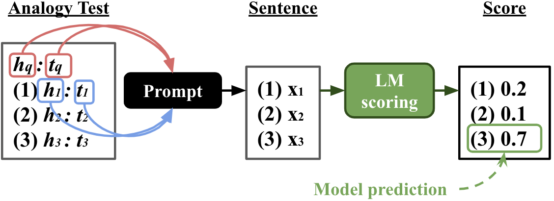
Figure 1: Solving a word analogy problem by selecting one with the highest LM score among the candidates.

In this section, we explain our strategy for using pretrained LMs to solve analogy problems without fine-tuning. First, in Section 4.1 we explain how each relation pair is converted into a natural sentence to be fed into the LM. In Section 4.2, we then discuss a number of scoring functions that can be used to select the most plausible answer candidate. Finally, we take advantage of the fact that analogical proportion is invariant to particular permutations, which allows for a natural extension of the proposed scoring functions (Section 4.3). Figure 1 shows a high-level overview of our methodology.

4.1 Relation Pair Prompting

We define a prompting function $\mathcal{T}_{t}(w_{1},w_{2},w_{3},w_{4})$ that takes four placeholders and a template type $t$, and returns a sentence in which the placeholders were replaced by the words $w_{1}$, $w_{2}$, $w_{3}$, and $w_{4}$. For instance, given a query “word:language” and a candidate “note:music”, the prompting function produces

$$\mathcal{T}_{\text{{\it to-as}}}(\text{``word"},\text{``language"},\text{``note"},\text{``music"})=\\ \text{``word is to language as note is to music"}$$

where we use the template type to-as here.

Using manually specified template types can result in a sub-optimal textual representation. For this reason, recent studies have proposed auto-prompting strategies, which optimize the template type on a training set Shin et al. (2020), paraphrasing Jiang et al. (2020), additional prompt generation model Gao et al. (2020), and corpus-driven template mining Bouraoui et al. (2020). However, none of these approaches can be applied to unsupervised settings. Thus, we do not explore auto-prompting methods in this work. Instead, we will consider a number of different template types in the experiments, and assess the sensitivity of the results to the choice of template type.

4.2 Scoring Function

Perplexity.  We first define perplexity, which is widely used as a sentence re-ranking metric Chan et al. (2016); Gulcehre et al. (2015). Given a sentence ${\boldsymbol{x}}$, for autoregressive LMs such as LSTM based models Zaremba et al. (2014) and GPTs Radford et al. (2018, 2019); Brown et al. (2020), perplexity can be computed as

$$f({\boldsymbol{x}})=\exp\left(-\sum_{j=1}^{m}\log{P_{\text{auto}}(x_{j}|{\boldsymbol{x}}_{j-1})}\right)$$ (1)

where ${\boldsymbol{x}}$ is tokenized as $[x_{1}...x_{m}]$ and $P_{\text{auto}}(x|{\boldsymbol{x}})$ is the likelihood from an autoregressive LM’s next token prediction. For masked LMs such as BERT Devlin et al. (2019) and RoBERTa Liu et al. (2019), we instead use pseudo-perplexity, which is defined as in (1) but with $P_{\text{mask}}(x_{j}|{\boldsymbol{x}}_{\backslash j})$ instead of $P_{\text{auto}}(x_{j}|{\boldsymbol{x}}_{j-1})$, where ${\boldsymbol{x}}_{\backslash j}=[x_{1}\dots x_{j_{1}}\text{\textlangle mask\textrangle}x_{j+1}\dots x_{m}]$ and $P_{\text{mask}}(x_{j}|{\boldsymbol{x}}_{\backslash j})$ is the pseudo-likelihood Wang and Cho (2019) that the masked token is $x_{j}$.

PMI.  Although perplexity is well-suited to capture the fluency of a sentence, it may not be the best choice to test the plausibility of a given analogical proportion candidate. As an alternative, we propose a scoring function that focuses specifically on words from the two given pairs. To this end, we propose to use an approximation of point-wise mutual information (PMI), based on perplexity.

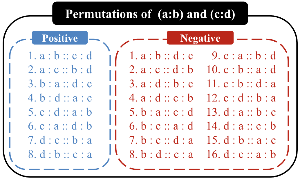
Figure 2: Positive and negative permutations for a relation pair (a:b)-(c:d).

PMI is defined as the difference between a conditional and marginal log-likelihood. In our case, we consider the conditional likelihood of $t_{i}$ given $h_{i}$ and the query pair (recall from Section 3.1 that $h$ and $t$ represent the head and tail of a given word pair, respectively), i.e. $P(t_{i}|h_{q},t_{q},h_{i})$, and the marginal likelihood over $h_{i}$, i.e. $P(t_{i}|h_{q},t_{q})$. Subsequently, the PMI-inspired scoring function is defined as

$$r(t_{i}|h_{i},h_{q},t_{q})= \log P(t_{i}|h_{q},t_{q},h_{i})$$

$$-\alpha\cdot\log P(t_{i}|h_{q},t_{q})$$ (2)

where $\alpha$ is a hyperparameter to control the effect of the marginal likelihood. The PMI score corresponds to the specific case where $\alpha=1$. However, Davison et al. (2019) found that using a hyperparameter to balance the impact of the conditional and marginal probabilities can significantly improve the results. The probabilities in (4.2) are estimated by assuming that the answer candidates are the only possible word pairs that need to be considered. By relying on this closed-world assumption, we can estimate marginal probabilities based on perplexity, which we found to give better results than the masking based strategy from Davison et al. (2019). In particular, we estimate these probabilities as

$$P(t_{i}|h_{q},t_{q},h_{i}) =-\frac{f\left(\mathcal{T}_{t}(h_{q},t_{q},h_{i},t_{i})\right)}{\sum\limits_{k=1}^{n}f\left(\mathcal{T}_{t}(h_{q},t_{q},h_{i},t_{k})\right)}$$

$$P(t_{i}|h_{q},t_{q}) =-\dfrac{\sum\limits_{k=1}^{n}f\left(\mathcal{T}_{t}(h_{q},t_{q},h_{k},t_{i})\right)}{\sum\limits_{k=1}^{n}\sum\limits_{l=1}^{n}f\left(\mathcal{T}_{t}(h_{q},t_{q},h_{k},t_{l})\right)}$$

where $n$ is the number of answer candidates for the given query. Equivalently, since PMI is symmetric, we can consider the difference between the logs of $P(h_{i}|h_{q},t_{q},t_{i})$ and $P(h_{i}|h_{q},t_{q})$. While this leads to the same PMI value in theory, due to the way in which we approximate the probabilities, this symmetric approach will lead to a different score. We thus combine both scores with an aggregation function $\mathcal{A}_{g}$. This aggregation function takes a list of scores and outputs an aggregated value. As an example, given a list $[1,2,3,4]$, we write $\mathcal{A}_{\text{mean}}([1,2,3,4])=2.5$ for the mean and $\mathcal{A}_{\text{val}_{1}}([1,2,3,4])=1$ for the first element. Given such an aggregation function, we define the following PMI-based score

$$s_{\textit{PMI}}(t_{i},h_{i}|h_{q},t_{q})=\mathcal{A}_{g}\left(\boldsymbol{r}\right)$$ (3)

where we consider basic aggregation operations over the list $\boldsymbol{r}=\left[r(t_{i}|h_{i},h_{q},t_{q}),r(h_{i}|t_{i},h_{q},t_{q})\right]$, such as the mean, max, and min value. The choice of using only one of the scores $r(t_{i}|h_{i},h_{q},t_{q})$, $r(h_{i}|t_{i},h_{q},t_{q})$ is viewed as a special case, in which the aggregation function $g$ simply returns the first or the second item.

mPPL.  We also experiment with a third scoring function, which borrows ideas from both perplexity and PMI. In particular, we propose the marginal likelihood biased perplexity (mPPL) defined as

$$s_{\textit{mPPL}}(t_{i},h_{i}|h_{q},t_{q})= \log s_{\textit{PPL}}(t_{i},h_{i}|h_{q},t_{q})$$

$$-\alpha_{t}\cdot\log P(t_{i}|h_{q},t_{q})$$

$$-\alpha_{h}\cdot\log P(h_{i}|h_{q},t_{q})$$

where $\alpha_{t}$ and $\alpha_{h}$ are hyperparameters, and ${s_{\textit{PPL}}}$ is a normalized perplexity defined as

$$s_{\textit{PPL}}(t_{i},h_{i}|h_{q},t_{q}) =-\frac{f\left(\mathcal{T}_{t}(h_{q},t_{q},h_{i},t_{i})\right)}{\sum\limits_{k=1}^{n}f\left(\mathcal{T}_{t}(h_{q},t_{q},h_{k},t_{k})\right)}.$$

The mPPL score extends perplexity with two bias terms. It is motivated from the insight that treating $\alpha$ as a hyperparameter in (4.2) can lead to better results than fixing $\alpha=1$. By tuning $\alpha_{t}$ and $\alpha_{h}$, we can essentially influence to what extent answer candidates involving semantically similar words to the query pair should be favored.

4.3 Permutation Invariance

The formalization of analogical proportions dates back to Aristotle Barbot et al. (2019). According to the standard axiomatic characterization, whenever we have an analogical proportion $a:b::c:d$ (meaning “$a$ is to $b$ what $c$ is to $d$”), it also holds that $c:d::a:b$ and $a:c::b:d$ are analogical proportions. It follows from this that for any given analogical proportion $a:b::c:d$ there are eight permutations of the four elements $a,b,c,d$ that form analogical proportions. These eight permutations, along with the 16 “negative permutations”, are shown in Figure 2.

To take advantage of the different permutations of analogical proportions, we propose the following Analogical Proportion (AP) score:

$$\textit{AP}(h_{q},t_{q},h_{i},t_{i}) =\mathcal{A}_{g_{\text{pos}}}(\boldsymbol{p})-\beta\cdot\mathcal{A}_{g_{\text{neg}}}(\boldsymbol{n})$$ (4)

$$\boldsymbol{p} =\left[s({a},{b}|{c},{d})\right]_{({a}:{b},{c}:{d})\in\boldsymbol{P}}$$

$$\boldsymbol{n} =\left[s({a},{b}|{c},{d})\right]_{({a}:{b},{c}:{d})\in\boldsymbol{N}}$$

where $\boldsymbol{P}$ and $\boldsymbol{N}$ correspond to the list of positive and negative permutations of the candidate analogical proportion $h_{q}:t_{q}::h_{i}:t_{i}$ in the order shown in Figure 2, $\beta$ is a hyperparameter to control the impact of the negative permutations, and $s(a,b|c,d)$ is a scoring function as described in Section 4.2. Here $\mathcal{A}_{g_{\text{pos}}}$ and $\mathcal{A}_{g_{\text{neg}}}$ refer to the aggregation functions that are used to combine the scores for the positive and negative permutations respectively, where these aggregation functions are defined as in Section 4.2. To solve an analogy problem, we simply choose the answer candidate that results in the highest value of $\textit{AP}(t_{i},h_{i},h_{q},t_{q})$.

5 Evaluation

In this section, we evaluate language models on the five analogy datasets presented in Section 3.

Model		Score	Tuned	SAT	U2	U4	Google	BATS	Avg
LM	BERT	$s_{\textit{PPL}}$		32.9	32.9	34.0	80.8	61.5	48.4
			✓	39.8	41.7	41.0	86.8	67.9	55.4
		$s_{\textit{PMI}}$		27.0	32.0	31.2	74.0	59.1	44.7
			✓	40.4	42.5	27.8	87.0	68.1	53.2
		$s_{\textit{mPPL}}$	✓	41.8	44.7	41.2	88.8	67.9	56.9
	GPT-2	$s_{\textit{PPL}}$		35.9	41.2	44.9	80.4	63.5	53.2
			✓	50.4	48.7	51.2	93.2	75.9	63.9
		$s_{\textit{PMI}}$		34.4	44.7	43.3	62.8	62.8	49.6
			✓	51.0	37.7	50.5	91.0	79.8	62.0
		$s_{\textit{mPPL}}$	✓	56.7	50.9	49.5	95.2	81.2	66.7
	RoBERTa	$s_{\textit{PPL}}$		42.4	49.1	49.1	90.8	69.7	60.2
			✓	53.7	57.0	55.8	93.6	80.5	68.1
		$s_{\textit{PMI}}$		35.9	42.5	44.0	60.8	60.8	48.8
			✓	51.3	49.1	38.7	92.4	77.2	61.7
		$s_{\textit{mPPL}}$	✓	53.4	58.3	57.4	93.6	78.4	68.2
WE	FastText	-		47.8	43.0	40.7	96.6	72.0	60.0
	GloVe	-		47.8	46.5	39.8	96.0	68.7	59.8
	Word2vec	-		41.8	40.4	39.6	93.2	63.8	55.8
Base	PMI	-		23.3	32.9	39.1	57.4	42.7	39.1
	Random	-		20.0	23.6	24.2	25.0	25.0	23.6

Table 3: Accuracy results on each analogy dataset, categorized into language models (LM), word embeddings (WE), and baselines (Base). All LMs use the analogical proportion (AP) function described in Section 4.3. The default configuration for AP includes $\alpha=\alpha_{h}=\alpha_{t}=\beta=0$, $g_{\text{pos}}=g=\text{val}_{1}$, and $t=\text{{\it to-as}}$. Note that $s_{\textit{PPL}}=s_{\textit{mPPL}}$ with the default configuration. Average accuracy (Avg) across datasets is included in the last column.

	Model	Score	Tuned	Accuracy
LM	BERT	$s_{\textit{PPL}}$		32.6
			✓	40.4*
		$s_{\textit{PMI}}$		26.8
			✓	41.2*
		$s_{\textit{mPPL}}$	✓	42.8*
	GPT-2	$s_{\textit{PPL}}$		41.4
			✓	56.2*
		$s_{\textit{PMI}}$		34.7
			✓	56.8*
		$s_{\textit{mPPL}}$	✓	57.8*
	RoBERTa	$s_{\textit{PPL}}$		49.6
			✓	55.8*
		$s_{\textit{PMI}}$		42.5
			✓	54.0*
		$s_{\textit{mPPL}}$	✓	55.8*
	GPT-3	Zero-shot		53.7
		Few-shot	✓	65.2*
-	LRA	-		56.4
WE	FastText	-		49.7
	GloVe	-		48.9
	Word2vec	-		42.8
Base	PMI	-		23.3
	Random	-		20.0

Table 4: Accuracy results for the full SAT dataset. Results marked with * are not directly comparable as they were tuned on full data (for our models) or use training data (for GPT-3 few-shot). These results are included to provide an upper bound only. Results in italics were taken from the original papers.

5.1 Experimental Setting

We consider three transformer-based LMs of a different nature: two masked LMs, namely BERT Devlin et al. (2019) and RoBERTa Liu et al. (2019), and GPT-2, as a prominent example of an auto-regressive language model. Each pretrained model was fetched from the Huggingface transformers library (Wolf et al., 2019), from which we use bert-large-cased, roberta-large, and gpt2-xl respectively. For parameter selection, we run grid search on $\beta$, $\alpha$, $\alpha_{h}$, $\alpha_{t}$, $t$, $g$, $g_{\text{{\it pos}}}$, and $g_{\text{{\it neg}}}$ for each model and select the configuration which achieves the best accuracy on each validation set. We experiment with the three scoring functions presented in Section 4.2, i.e., $s_{\textit{PPL}}$ (perplexity), $s_{\textit{PMI}}$ and $s_{\textit{mPPL}}$. Possible values for each hyperparameter (including the selection of six prompts and an ablation test on the scoring function) and the best configurations that were found by grid search are provided in the appendix.

As baseline methods, we also consider three pre-trained word embedding models, which have been shown to provide competitive results in analogy tasks, as explained in Section 2.2: Word2vec Mikolov et al. (2013a), GloVe Pennington et al. (2014), and FastText Bojanowski et al. (2017). For the word embedding models, we simply represent word pairs by taking the difference between their embeddings. We then choose the answer candidate with the highest cosine similarity to the query in terms of this vector difference. To put the results into context, we also include two simple statistical baselines. First, we report the expected random performance. Second, we use a method based on each word pair’s PMI in a given corpus. We then select the answer candidate with the highest PMI as the prediction. Note that the query word pair is completely ignored in this case. This PMI score is the well-known word-pair association metric introduced by Church and Hanks (1990) for lexicographic purposes (specifically, collocation extraction), which compares the probability of observing two words together with the probabilities of observing them independently (chance). The PMI scores in our experiments were computed using the English Wikipedia with a fixed window size 10.

5.2 Results

Table 3 shows our main results. As far as the comparison among LMs is concerned, RoBERTa and GPT-2 consistently outperform BERT. Among the AP variants, $s_{\textit{mPPL}}$ achieves substantially better results than $s_{\textit{PMI}}$ or $s_{\textit{PPL}}$ in most cases. We also observe that word embeddings perform surprisingly well, with FastText and GloVe outperforming BERT on most datasets, as well as GPT-2 and RoBERTa with default hyperparameters. FastText achieves the best overall accuracy on the Google dataset, confirming that this dataset is particularly well-suited to word embeddings (see Section 2.2).

In order to compare with published results from prior work, we carried out an additional experiment on the full SAT dataset (i.e., without splitting it into validation and test). Table 4 shows the results. GPT-3 Brown et al. (2020) and LRA Turney (2005) are added for comparison. Given the variability of the results depending on the tuning procedure, we have also reported results of configurations that were tuned on the entire set, to provide an upper bound on what is possible within the proposed unsupervised setting. This result shows that even with optimal hyperparameter values, LMs barely outperform the performance of the simpler LRA model. GPT-3 similarly fails to outperform LRA in the zero-shot setting.

6 Analysis

We now take a closer look into our results to investigate parameter sensitivity, the correlation between model performance and human difficulty levels, and possible dataset artifacts. The following analysis focuses on $s_{\textit{mPPL}}$ as it achieved the best results among the LM based scoring functions.

Parameter Sensitivity

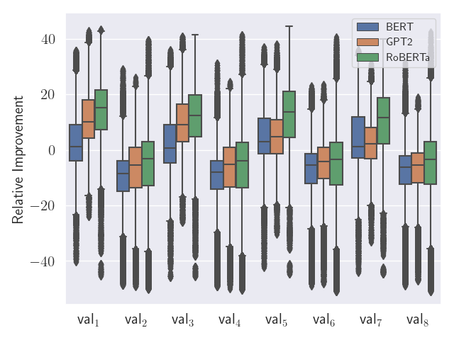
Figure 3: Box plot of the relative improvement on test accuracy in each dataset over all configurations of $s_{\textit{mPPL}}$ grouped by $g_{\text{pos}}$. Here val_k corresponds to $k$th positive permutation shown in Figure 2.

We found that optimal values of the parameters $\alpha$ and $\beta$ are highly dependent on the dataset, while other parameters such as the template type $t$ vary across LMs. On the other hand, as shown in Figure 3, the optimal permutations of the templates are relatively consistent, with the original ordering $a:b::c:d$ typically achieving the best results. The results degrade most for permutations that mix the two word pairs (e.g. $a:c::b:d$). In the appendix we include an ablation study for the sensitivity and relevance of other parameters and design choices.

Difficulty Levels

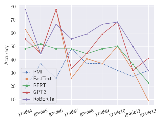
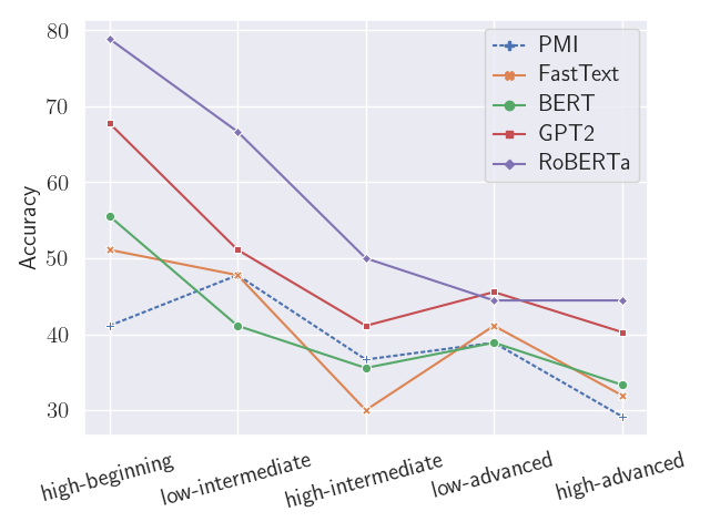
Figure 4: Test accuracy in U2 and U4 per difficulty level. LMs use $s_{\textit{mPPL}}$ with the best configuration tuned in the corresponding validation sets.

To increase our understanding of what makes an analogy problem difficult for LMs, we compare the results for each difficulty level. Recall from Section 3.2 that the U2 and U4 datasets come from educational resources and are split by difficulty level. Figure 4 shows the results of all LMs (tuned setting), FastText and the PMI baseline according to these difficulty levels. Broadly speaking, we can see that instances that are harder for humans are also harder for the considered models. The analogies in the most difficult levels are generally more abstract (e.g. $\textit{witness}:\textit{testimony}::\textit{generator}:\textit{electricity}$), or contain obscure or infrequent words (e.g. $\textit{grouch}:\textit{cantakerous}::\textit{palace}:\textit{ornate}$).

Hypothesis Only

Recently, several researchers have found that standard NLP benchmarks, such as SNLI Bowman et al. (2015) for language inference, contain several annotation artifacts that makes the task simpler for automatic models Poliak et al. (2018); Gururangan et al. (2018). One of their most relevant findings is that models which do not even consider the premise can reach high accuracy. More generally, these issues have been found to be problematic in NLP models Linzen (2020) and neural networks more generally Geirhos et al. (2020). According to the results shown in Table 3, we already found that the PMI baseline achieved a non-trivial performance, even outperforming BERT in a few settings and datasets. This suggests that several implausible negative examples are included in the analogy datasets. As a further exploration of such artifacts, here we analyse the analogue of a hypothesis-only baseline. In particular, for this analysis, we masked the head or tail of the candidate answer in all evaluation instances. Then, we test the masked language models with the same AP configuration and tuning on these artificially-modified datasets.As can be seen in Table 5, a non-trivial performance is achieved for all datasets, which suggests that the words from the answer pair tend to be more similar to the words from the query than the words from negative examples.

	Mask	SAT	U2	U4	Google	BATS
BERT	full	41.8	44.7	41.2	88.8	67.9
	head	31.8	28.1	34.3	72.0	62.4
	tail	33.5	31.6	38.2	64.2	63.1
RoBERTa	full	53.4	58.3	57.4	93.6	78.4
	head	38.6	37.7	41.0	60.6	54.5
	tail	35.6	37.3	40.5	55.8	64.2

Table 5: Accuracy results by masking head or tail of the candidate answers. Results in the top row correspond to the full model without masking.

7 Conclusion

In this paper, we have presented an extensive analysis of the ability of language models to identify analogies. To this end, we first compiled datasets with psychometric analogy problems from educational resources, covering a wide range of difficulty levels and topics. We also recast two standard benchmarks, the Google and BATS analogy datasets, into the same style of problems. Then, we proposed standard techniques to apply language models to the unsupervised task of solving these analogy problems. Our empirical results shed light on the strengths and limitations of various models. To directly answer the question posed in the title, our conclusion is that language models can identify analogies to a certain extent, but not all language models are able to achieve a meaningful improvement over word embeddings (whose limitations in analogy tasks are well documented). On the other hand, when carefully tuned, some language models are able to achieve state-of-the-art results. We emphasize that results are highly sensitive to the chosen hyperparameters (which define the scoring function and the prompt among others). Further research could focus on the selection of these optimal hyperparameters, including automatizing the search or generation of prompts, along the lines of Bouraoui et al. (2020) and Shin et al. (2020), respectively. Finally, clearly LMs might still be able to learn to solve analogy tasks when given appropriate training data, which is an aspect that we leave for future work.

Appendix A Experimental Details

In our grid search to find the optimal configuration for each dataset and language model, each parameter was selected within the values shown in Table 6. As the coefficient of marginal likelihood $\alpha,\alpha_{h},\alpha_{t}$, we considered negative values as well as we hypothesized that the marginal likelihood could be beneficial for LMs as a way to leverage lexical knowledge of the head and tail words.

Additionally, Table 7 shows the set of custom templates (or prompts) used in our experiments. Finally, Tables 8, 9, and 10 include the best configuration based on each validation set in for $s_{\textit{PMI}}$, $s_{\textit{mPPL}}$ and the hypothesis-only baseline, respectively.

Parameter	Value
$\alpha$	-0.4, -0.2, 0, 0.2, 0.4
$\alpha_{h}$	-0.4, -0.2, 0, 0.2, 0.4
$\alpha_{t}$	-0.4, -0.2, 0, 0.2, 0.4
$\beta$	0, 0.2, 0.4, 0.6, 0.8, 1.0
$g$	max,mean,min,val1,val2
$g_{\text{pos}}$	max,mean,min,val1,…,val8
$g_{\text{neg}}$	max,mean,min,val1,…,val16

Table 6: Hyperparameters with each search space.

Type	Template
to-as	[$w_{1}$] is to [$w_{2}$] as [$w_{3}$] is to [$w_{4}$]
to-what	[$w_{1}$] is to [$w_{2}$] What [$w_{3}$] is to [$w_{4}$]
rel-same	The relation between [$w_{1}$] and [$w_{2}$]
	is the same as the relation between
	[$w_{3}$] and [$w_{4}$].
what-to	what [$w_{1}$] is to [$w_{2}$], [$w_{3}$] is to [$w_{4}$]
she-as	She explained to him that [$w_{1}$] is
	to [$w_{2}$] as [$w_{3}$] is to [$w_{4}$]
as-what	As I explained earlier, what [$w_{1}$] is
	to [$w_{2}$] is essentially the same as
	what [$w_{3}$] is to [$w_{4}$].

Table 7: Custom templates used in our experiments. Each has four placeholders $[w_{1},...,w_{4}]$ and they are fulfilled by words from a relation pair.

	Data	$g$	$\alpha$	$g_{\text{pos}}$	$g_{\text{neg}}$	$\beta$	$t$
BERT	SAT	val2	-0.4	val5	val12	0.4	what-to
	U2	val2	-0.4	mean	mean	0.6	what-to
	U4	val1	0.4	max	val7	1.0	rel-same
	Google	val1	-0.4	val1	val11	0.4	she-as
	BATS	val1	-0.4	val11	val1	0.4	she-as
GPT-2	SAT	val2	-0.4	val3	val1	0.6	rel-same
	U2	val2	0.0	val4	val4	0.6	rel-same
	U4	val2	-0.4	mean	mean	0.6	rel-same
	Google	val1	0.0	mean	val11	0.4	as-what
	BATS	val1	-0.4	val1	val6	0.4	rel-same
RoBERTa	SAT	min	-0.4	min	val7	0.2	as-what
	U2	min	0.4	mean	val4	0.6	what-to
	U4	val2	0.0	mean	val4	0.8	to-as
	Google	val1	-0.4	val1	val6	0.4	what-to
	BATS	max	-0.4	mean	val11	0.6	what-to

Table 8: The best configuration of $s_{\textit{PMI}}$ score.

	Data	$\alpha_{h}$	$\alpha_{t}$	$g_{\text{pos}}$	$g_{\text{neg}}$	$\beta$	$t$
BERT	SAT	-0.2	-0.4	val5	val5	0.2	what-to
	U2	0.0	-0.2	mean	mean	0.8	she-as
	U4	-0.2	0.4	val7	min	0.4	to-as
	Google	0.4	-0.2	val5	val12	0.6	she-as
	BATS	0.0	0.0	val8	min	0.4	what-to
GPT-2	SAT	-0.4	0.2	val3	val1	0.8	rel-same
	U2	-0.2	0.2	mean	mean	0.8	as-what
	U4	-0.2	0.2	mean	mean	0.8	rel-same
	Google	-0.2	-0.4	mean	mean	0.8	rel-same
	BATS	0.4	-0.4	val1	val5	0.8	rel-same
RoBERTa	SAT	0.2	0.2	val5	val11	0.2	as-what
	U2	0.4	0.4	val1	val4	0.4	what-to
	U4	0.2	0.2	val1	val1	0.4	as-what
	Google	0.2	0.2	val1	val6	0.2	what-to
	BATS	0.2	-0.2	val5	val11	0.4	what-to

Table 9: The best configuration of $s_{\textit{mPPL}}$ score.

	Mask	Data	$g_{\text{{\it pos}}}$	$t$
BERT	head	SAT	val5	to-what
		U2	val5	to-as
		U4	mean	to-as
		Google	val5	she-as
		BATS	val5	to-as
	tail	SAT	val3	what-to
		U2	val7	to-what
		U4	val4	rel-same
		Google	val7	as-what
		BATS	val7	to-as
RoBERTa	head	SAT	val5	as-what
		U2	val5	rel-same
		U4	val7	she-as
		Google	val5	what-to
		BATS	val5	she-as
	tail	SAT	mean	what-to
		U2	val7	rel-same
		U4	mean	what-to
		Google	val7	as-what
		BATS	val7	what-to

Table 10: The best configurations for hypothesis-only scores.

Appendix B Additional Ablation Results

We show a few more complementary results to our main experiments.

B.1 Alternative Scoring Functions

As alternative scoring functions for LM, we have tried two other scores: PMI score based on masked token prediction Davison et al. (2019) (Mask PMI) and cosine similarity between the embedding difference of a relation pair similar to what used in word-embedding models. For embedding method, we give a prompted sentence to LM to get the last layer’s hidden state for each word in the given pair and we take the difference between them, which we regard as the embedding vector for the pair. Finally we pick up the most similar candidate in terms of the cosine similarity with the query embedding. Table 11 shows the test accuracy on each dataset. As one can see, AP scores outperform other methods with a great margin.

	Score	SAT	U2	U4	Google	BATS
BERT	embedding	24.0	22.4	26.6	28.2	28.3
	Mask PMI	25.2	23.3	31.5	61.2	46.2
	$s_{\textit{PMI}}$	40.4	42.5	27.8	87.0	68.1
	$s_{\textit{mPPL}}$	41.8	44.7	41.2	88.8	67.9
RoBERTa	embedding	40.4	42.5	27.8	87.0	68.1
	Mask PMI	43.0	36.8	39.4	69.2	58.3
	$s_{\textit{PMI}}$	51.3	49.1	38.7	92.4	77.2
	$s_{\textit{mPPL}}$	53.4	58.3	57.4	93.6	78.4

Table 11: Test accuracy tuned on each validation set.

B.2 Parameter Sensitivity: template type $t$

Figure 5 shows the box plot of relative improvement across all datasets grouped by $t$ and the results indicate that there is a mild trend that certain templates tend to perform well, but not significant universal selectivity can be found across datasets.

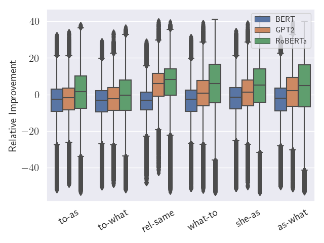
Figure 5: Box plot of the relative improvement on test accuracy in each dataset over all configurations of $s_{\textit{mPPL}}$ grouped by template type.

B.3 Parameter Sensitivity: aggregation method $g_{\text{neg}}$

Figure 6 shows the box plot of relative improvement across all datasets grouped by $g_{\text{neg}}$. Unlike $g_{\text{pos}}$ we show in Figure 3, they do not give a strong signals over datasets.

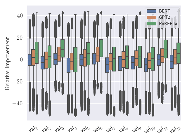
Figure 6: Box plot of the relative improvement on test accuracy in each dataset over all configurations of $s_{\textit{mPPL}}$ grouped by $g_{\text{neg}}$. Here val_k corresponds to $k$th positive permutation shown in Figure 2.

B.4 Relation Types in BATS/Google

Figure 7 shows the results of different language models with the $s_{\textit{mPPL}}$ scoring function on the different categories of the BATS and Google datasets.

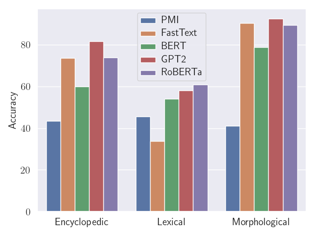
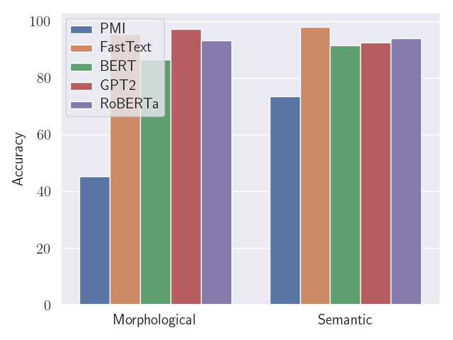
Figure 7: BATS (top) and Google (bottom) results split by high-level categories.

Appendix C Error Analysis

Table 12 shows all examples from the U2 dataset of the easiest difficuly (i.e. grade 4), which were misclassified by RoBERTa, with $s_{\textit{mPPL}}$ tuned on the validation set. We can see a few typical issues with word embeddings and language models. For instance, in the first example, the model confuses the antonym pair right:wrong with synonymy. In the second example, we have that someone who is poor lacks money, while someone who is hungry lacks food. However, the selected candidate pair is hungy:water rather than hungry:food, which is presumably chosen because water is assumed to be a near-synonym of food. In the third example (wrench:tool), the hypnernymy relation is confused with a meronymy relation in the selected candidate tree:forest. In the last three examples, the model has selected answers which seem reasonable. In the fourth example, beautiful:pretty, terrible:bad and brave:valiant can all be considered to be synonym pairs. In the fifth example, vehicle:transport is clearly the correct answer, but the pair song:sing is nonetheless relationally similar to shield:protect. In the last example, we can think of being sad as an emotional state, like being sick is a health state, which provides some justification for the predicted answer. On the other hand, the gold answer is based on the argument that someone who is sick lacks health like someone who is scared lacks courage.

Query	Candidates
hilarious:funny	right:wrong, hard:boring, nice:crazy,
	great:good
poor:money	tired:energy, angry:emotion, hot:ice,
	hungry:water
wrench:tool	cow:milk, radio:sound, tree:forest,
	carrot:vegetable
beautiful:pretty	terrible:bad, brave:valiant, new:old,
	tall:skinny
shield:protect	computer:talk, vehicle:transport,
	pencil:make, song:sing
sick:health	sad:emotion, tall:intelligence,
	scared:courage, smart:energy

Table 12: Model prediction examples from RoBERTa with $s_{\textit{mPPL}}$ tuned on the validation set. Gold answers are shown in bold, while the model predictions are underlined.

References

- Allen and Hospedales (2019) Carl Allen and Timothy Hospedales. 2019. Analogies explained: Towards understanding word embeddings. In International Conference on Machine Learning, pages 223–231.
- Arora et al. (2016) Sanjeev Arora, Yuanzhi Li, Yingyu Liang, Tengyu Ma, and Andrej Risteski. 2016. A latent variable model approach to pmi-based word embeddings. Transactions of the Association for Computational Linguistics, 4:385–399.
- Ashley (1988) Kevin D Ashley. 1988. Arguing by analogy in law: A case-based model. In Analogical reasoning, pages 205–224. Springer.
- Barbot et al. (2019) Nelly Barbot, Laurent Miclet, and Henri Prade. 2019. Analogy between concepts. Artificial Intelligence, 275:487–539.
- Bojanowski et al. (2017) Piotr Bojanowski, Edouard Grave, Armand Joulin, and Tomas Mikolov. 2017. Enriching word vectors with subword information. Transactions of the Association of Computational Linguistics, 5(1):135–146.
- Bolukbasi et al. (2016) Tolga Bolukbasi, Kai-Wei Chang, James Y Zou, Venkatesh Saligrama, and Adam T Kalai. 2016. Man is to computer programmer as woman is to homemaker? debiasing word embeddings. In Advances in Neural Information Processing Systems, pages 4349–4357.
- Boteanu and Chernova (2015) Adrian Boteanu and Sonia Chernova. 2015. Solving and explaining analogy questions using semantic networks. In Proceedings of the AAAI Conference on Artificial Intelligence.
- Bouraoui et al. (2020) Zied Bouraoui, Jose Camacho-Collados, and Steven Schockaert. 2020. Inducing relational knowledge from bert. In Proceedings of the AAAI Conference on Artificial Intelligence, volume 34, pages 7456–7463.
- Bouraoui et al. (2018) Zied Bouraoui, Shoaib Jameel, and Steven Schockaert. 2018. Relation induction in word embeddings revisited. In Proceedings of the 27th International Conference on Computational Linguistics, pages 1627–1637, Santa Fe, New Mexico, USA. Association for Computational Linguistics.
- Bowman et al. (2015) Samuel R. Bowman, Gabor Angeli, Christopher Potts, and Christopher D. Manning. 2015. A large annotated corpus for learning natural language inference. In Proceedings of the 2015 Conference on Empirical Methods in Natural Language Processing, pages 632–642, Lisbon, Portugal. Association for Computational Linguistics.
- Brown et al. (2020) Tom B. Brown, Benjamin Mann, Nick Ryder, Melanie Subbiah, Jared Kaplan, Prafulla Dhariwal, Arvind Neelakantan, Pranav Shyam, Girish Sastry, Amanda Askell, Sandhini Agarwal, Ariel Herbert-Voss, Gretchen Krueger, Tom Henighan, Rewon Child, Aditya Ramesh, Daniel M. Ziegler, Jeffrey Wu, Clemens Winter, Christopher Hesse, Mark Chen, Eric Sigler, Mateusz Litwin, Scott Gray, Benjamin Chess, Jack Clark, Christopher Berner, Sam McCandlish, Alec Radford, Ilya Sutskever, and Dario Amodei. 2020. Language models are few-shot learners. In Annual Conference on Neural Information Processing Systems.
- Chan et al. (2016) William Chan, Navdeep Jaitly, Quoc Le, and Oriol Vinyals. 2016. Listen, attend and spell: A neural network for large vocabulary conversational speech recognition. In 2016 IEEE International Conference on Acoustics, Speech and Signal Processing (ICASSP), pages 4960–4964. IEEE.
- Chiang et al. (2020) Hsiao-Yu Chiang, Jose Camacho-Collados, and Zachary Pardos. 2020. Understanding the source of semantic regularities in word embeddings. In Proceedings of the 24th Conference on Computational Natural Language Learning, pages 119–131, Online. Association for Computational Linguistics.
- Church and Hanks (1990) Kenneth Church and Patrick Hanks. 1990. Word association norms, mutual information, and lexicography. Computational linguistics, 16(1):22–29.
- Davison et al. (2019) Joe Davison, Joshua Feldman, and Alexander M Rush. 2019. Commonsense knowledge mining from pretrained models. In Proceedings of the 2019 Conference on Empirical Methods in Natural Language Processing and the 9th International Joint Conference on Natural Language Processing, pages 1173–1178.
- Devlin et al. (2019) Jacob Devlin, Ming-Wei Chang, Kenton Lee, and Kristina Toutanova. 2019. Bert: Pre-training of deep bidirectional transformers for language understanding. In Proceedings of the 2019 Conference of the North American Chapter of the Association for Computational Linguistics: Human Language Technologies, Volume 1 (Long and Short Papers), pages 4171–4186.
- Drozd et al. (2016) Aleksandr Drozd, Anna Gladkova, and Satoshi Matsuoka. 2016. Word embeddings, analogies, and machine learning: Beyond king-man+ woman= queen. In Proceedings of coling 2016, the 26th international conference on computational linguistics: Technical papers, pages 3519–3530.
- Ethayarajh et al. (2019) Kawin Ethayarajh, David Duvenaud, and Graeme Hirst. 2019. Towards understanding linear word analogies. In Proceedings of the 57th Annual Meeting of the Association for Computational Linguistics, pages 3253–3262.
- Ettinger (2019) Allyson Ettinger. 2019. What bert is not: Lessons from a new suite of psycholinguistic diagnostics for language models. Transactions of the Association for Computational Linguistics, 8:34–48.
- Feldman and Ballard (1982) Jerome A. Feldman and Dana H. Ballard. 1982. Connectionist models and their properties. Cognitive Science, 6(3):205–254.
- Fournier et al. (2020) Louis Fournier, Emmanuel Dupoux, and Ewan Dunbar. 2020. Analogies minus analogy test: measuring regularities in word embeddings. In Proceedings of the 24th Conference on Computational Natural Language Learning, pages 365–375, Online. Association for Computational Linguistics.
- Gao et al. (2020) Tianyu Gao, Adam Fisch, and Danqi Chen. 2020. Making pre-trained language models better few-shot learners. arXiv preprint arXiv:2012.15723.
- Geirhos et al. (2020) Robert Geirhos, Jörn-Henrik Jacobsen, Claudio Michaelis, Richard Zemel, Wieland Brendel, Matthias Bethge, and Felix A Wichmann. 2020. Shortcut learning in deep neural networks. Nature Machine Intelligence, 2(11):665–673.
- Gittens et al. (2017) Alex Gittens, Dimitris Achlioptas, and Michael W Mahoney. 2017. Skip-gram- zipf+ uniform= vector additivity. In Proceedings of the 55th Annual Meeting of the Association for Computational Linguistics (Volume 1: Long Papers), pages 69–76.
- Gladkova et al. (2016) Anna Gladkova, Aleksandr Drozd, and Satoshi Matsuoka. 2016. Analogy-based detection of morphological and semantic relations with word embeddings: what works and what doesn’t. In Proceedings of the Student Research Workshop at NAACL, pages 8–15.
- Goel (2019) Ashok Goel. 2019. Computational design, analogy, and creativity. In Computational Creativity, pages 141–158. Springer.
- Goldberg (2019) Yoav Goldberg. 2019. Assessing bert’s syntactic abilities. arXiv preprint arXiv:1901.05287.
- Gonen and Goldberg (2019) Hila Gonen and Yoav Goldberg. 2019. Lipstick on a pig: Debiasing methods cover up systematic gender biases in word embeddings but do not remove them. In Proceedings of the 2019 Conference of the North American Chapter of the Association for Computational Linguistics: Human Language Technologies, Volume 1 (Long and Short Papers), pages 609–614.
- Gulcehre et al. (2015) Caglar Gulcehre, Orhan Firat, Kelvin Xu, Kyunghyun Cho, Loic Barrault, Huei-Chi Lin, Fethi Bougares, Holger Schwenk, and Yoshua Bengio. 2015. On using monolingual corpora in neural machine translation. arXiv preprint arXiv:1503.03535.
- Gururangan et al. (2018) Suchin Gururangan, Swabha Swayamdipta, Omer Levy, Roy Schwartz, Samuel Bowman, and Noah A. Smith. 2018. Annotation artifacts in natural language inference data. In Proceedings of the 2018 Conference of the North American Chapter of the Association for Computational Linguistics: Human Language Technologies, Volume 2 (Short Papers), pages 107–112, New Orleans, Louisiana. Association for Computational Linguistics.
- Hakami and Bollegala (2017) Huda Hakami and Danushka Bollegala. 2017. Compositional approaches for representing relations between words: A comparative study. Knowledge-Based Systems, 136:172–182.
- Hewitt and Manning (2019) John Hewitt and Christopher D. Manning. 2019. A structural probe for finding syntax in word representations. In Proceedings of the 2019 Conference of the North American Chapter of the Association for Computational Linguistics: Human Language Technologies, Volume 1 (Long and Short Papers), pages 4129–4138, Minneapolis, Minnesota. Association for Computational Linguistics.
- Hinton (1986) Geoffrey E. Hinton. 1986. Learning distributed representations of concepts. In Proceedings of the eighth annual conference of the cognitive science society, volume 1, page 12. Amherst, MA.
- Hinton et al. (1986) Geoffrey E. Hinton, James L. McClelland, and David E. Rumelhart. 1986. Distributed representations. Parallel distributed processing: explorations in the microstructure of cognition, vol. 1, pages 77–109.
- Holyoak et al. (1996) Keith J Holyoak, Keith James Holyoak, and Paul Thagard. 1996. Mental leaps: Analogy in creative thought. MIT press.
- Hope et al. (2017) Tom Hope, Joel Chan, Aniket Kittur, and Dafna Shahaf. 2017. Accelerating innovation through analogy mining. In Proceedings of the 23rd ACM SIGKDD International Conference on Knowledge Discovery and Data Mining, pages 235–243.
- Hopfield (1982) John J. Hopfield. 1982. Neural networks and physical systems with emergent collective computational abilities. Proceedings of the National Academy of Sciences, 79(8):2554–2558.
- Hug et al. (2016) Nicolas Hug, Henri Prade, Gilles Richard, and Mathieu Serrurier. 2016. Analogical classifiers: a theoretical perspective. In Proceedings of the Twenty-second European Conference on Artificial Intelligence, pages 689–697.
- Hüllermeier (2020) Eyke Hüllermeier. 2020. Towards analogy-based explanations in machine learning. In International Conference on Modeling Decisions for Artificial Intelligence, pages 205–217.
- Jawahar et al. (2019) Ganesh Jawahar, Benoît Sagot, and Djamé Seddah. 2019. What does BERT learn about the structure of language? In Proceedings of the 57th Annual Meeting of the Association for Computational Linguistics, pages 3651–3657, Florence, Italy. Association for Computational Linguistics.
- Jiang et al. (2020) Zhengbao Jiang, Frank F. Xu, Jun Araki, and Graham Neubig. 2020. How can we know what language models know? Transactions of the Association for Computational Linguistics, 8:423–438.
- Landauer and Dumais (1997) Thomas K. Landauer and Susan T. Dumais. 1997. A solution to Plato’s problem: The latent semantic analysis theory of acquisition, induction, and representation of knowledge. Psychological Review, 104(2):211.
- Levy and Goldberg (2014) Omer Levy and Yoav Goldberg. 2014. Linguistic regularities in sparse and explicit word representations. In Proceedings of the Eighteenth Conference on Computational Natural Language Learning, pages 171–180, Ann Arbor, Michigan. Association for Computational Linguistics.
- Linzen (2016) Tal Linzen. 2016. Issues in evaluating semantic spaces using word analogies. In Proceedings of the 1st Workshop on Evaluating Vector-Space Representations for NLP, pages 13–18.
- Linzen (2020) Tal Linzen. 2020. How can we accelerate progress towards human-like linguistic generalization? In Proceedings of the 58th Annual Meeting of the Association for Computational Linguistics, pages 5210–5217, Online. Association for Computational Linguistics.
- Liu et al. (2019) Yinhan Liu, Myle Ott, Naman Goyal, Jingfei Du, Mandar Joshi, Danqi Chen, Omer Levy, Mike Lewis, Luke Zettlemoyer, and Veselin Stoyanov. 2019. Roberta: A robustly optimized BERT pretraining approach. CoRR, abs/1907.11692.
- Miclet et al. (2008) Laurent Miclet, Sabri Bayoudh, and Arnaud Delhay. 2008. Analogical dissimilarity: definition, algorithms and two experiments in machine learning. Journal of Artificial Intelligence Research, 32:793–824.
- Mikolov et al. (2013a) Tomas Mikolov, Ilya Sutskever, Kai Chen, Greg S Corrado, and Jeff Dean. 2013a. Distributed representations of words and phrases and their compositionality. In Advances in neural information processing systems, pages 3111–3119.
- Mikolov et al. (2013b) Tomas Mikolov, Wen-tau Yih, and Geoffrey Zweig. 2013b. Linguistic regularities in continuous space word representations. In Proceedings of HLT-NAACL, pages 746–751.
- Nissim et al. (2020) Malvina Nissim, Rik van Noord, and Rob van der Goot. 2020. Fair is better than sensational: Man is to doctor as woman is to doctor. Computational Linguistics, 46(2):487–497.
- Paperno and Baroni (2016) Denis Paperno and Marco Baroni. 2016. When the whole is less than the sum of its parts: How composition affects pmi values in distributional semantic vectors. Computational Linguistics, 42(2):345–350.
- Pardos and Nam (2020) Zachary A. Pardos and Andrew J. H. Nam. 2020. A university map of course knowledge. PLoS ONE, 15(9).
- Pennington et al. (2014) Jeffrey Pennington, Richard Socher, and Christopher D Manning. 2014. GloVe: Global vectors for word representation. In Proceedings of EMNLP, pages 1532–1543.
- Peters et al. (2018a) Matthew Peters, Mark Neumann, Mohit Iyyer, Matt Gardner, Christopher Clark, Kenton Lee, and Luke Zettlemoyer. 2018a. Deep contextualized word representations. In Proceedings of the 2018 Conference of the North American Chapter of the Association for Computational Linguistics: Human Language Technologies, Volume 1 (Long Papers), pages 2227–2237, New Orleans, Louisiana. Association for Computational Linguistics.
- Peters et al. (2018b) Matthew Peters, Mark Neumann, Luke Zettlemoyer, and Wen-tau Yih. 2018b. Dissecting contextual word embeddings: Architecture and representation. In Proceedings of the 2018 Conference on Empirical Methods in Natural Language Processing, pages 1499–1509, Brussels, Belgium. Association for Computational Linguistics.
- Petroni et al. (2019) Fabio Petroni, Tim Rocktäschel, Sebastian Riedel, Patrick Lewis, Anton Bakhtin, Yuxiang Wu, and Alexander Miller. 2019. Language models as knowledge bases? In Proceedings of the 2019 Conference on Empirical Methods in Natural Language Processing and the 9th International Joint Conference on Natural Language Processing (EMNLP-IJCNLP), pages 2463–2473.
- Poliak et al. (2018) Adam Poliak, Jason Naradowsky, Aparajita Haldar, Rachel Rudinger, and Benjamin Van Durme. 2018. Hypothesis only baselines in natural language inference. In Proceedings of the Seventh Joint Conference on Lexical and Computational Semantics, pages 180–191, New Orleans, Louisiana. Association for Computational Linguistics.
- Prade and Richard (2017) Henri Prade and Gilles Richard. 2017. Analogical proportions and analogical reasoning-an introduction. In International Conference on Case-Based Reasoning, pages 16–32. Springer.
- Raad and Evermann (2015) Elie Raad and Joerg Evermann. 2015. The role of analogy in ontology alignment: A study on lisa. Cognitive Systems Research, 33:1–16.
- Radford et al. (2018) Alec Radford, Karthik Narasimhan, Tim Salimans, and Ilya Sutskever. 2018. Improving language understanding by generative pre-training.
- Radford et al. (2019) Alec Radford, Jeff Wu, Rewon Child, David Luan, Dario Amodei, and Ilya Sutskever. 2019. Language models are unsupervised multitask learners.
- Rogers et al. (2021) Anna Rogers, Olga Kovaleva, and Anna Rumshisky. 2021. A primer in bertology: What we know about how bert works. Transactions of the Association for Computational Linguistics, 8:842–866.
- Saphra and Lopez (2019) Naomi Saphra and Adam Lopez. 2019. Understanding learning dynamics of language models with SVCCA. In Proceedings of the 2019 Conference of the North American Chapter of the Association for Computational Linguistics: Human Language Technologies, Volume 1 (Long and Short Papers), pages 3257–3267, Minneapolis, Minnesota. Association for Computational Linguistics.
- van Schijndel et al. (2019) Marten van Schijndel, Aaron Mueller, and Tal Linzen. 2019. Quantity doesn’t buy quality syntax with neural language models. In Proceedings of the 2019 Conference on Empirical Methods in Natural Language Processing and the 9th International Joint Conference on Natural Language Processing (EMNLP-IJCNLP), pages 5831–5837, Hong Kong, China. Association for Computational Linguistics.
- Schluter (2018) Natalie Schluter. 2018. The word analogy testing caveat. In Proceedings of the 2018 Conference of the North American Chapter of the Association for Computational Linguistics: Human Language Technologies, Volume 2 (Short Papers), pages 242–246.
- Shin et al. (2020) Taylor Shin, Yasaman Razeghi, Robert L. Logan IV, Eric Wallace, and Sameer Singh. 2020. AutoPrompt: Eliciting Knowledge from Language Models with Automatically Generated Prompts. In Proceedings of the 2020 Conference on Empirical Methods in Natural Language Processing (EMNLP), pages 4222–4235, Online. Association for Computational Linguistics.
- Tenney et al. (2019a) Ian Tenney, Dipanjan Das, and Ellie Pavlick. 2019a. BERT rediscovers the classical NLP pipeline. In Proceedings of the 57th Annual Meeting of the Association for Computational Linguistics, pages 4593–4601, Florence, Italy. Association for Computational Linguistics.
- Tenney et al. (2019b) Ian Tenney, Patrick Xia, Berlin Chen, Alex Wang, Adam Poliak, R. Thomas McCoy, Najoung Kim, Benjamin Van Durme, Samuel R. Bowman, Dipanjan Das, and Ellie Pavlick. 2019b. What do you learn from context? probing for sentence structure in contextualized word representations. In Proceeding of the 7th International Conference on Learning Representations (ICLR).
- Turney (2005) Peter D. Turney. 2005. Measuring semantic similarity by latent relational analysis. In Proc. of IJCAI, pages 1136–1141.
- Turney et al. (2003) Peter D. Turney, Michael L. Littman, Jeffrey Bigham, and Victor Shnayder. 2003. Combining independent modules in lexical multiple-choice problems. In Recent Advances in Natural Language Processing III, pages 101–110.
- Vylomova et al. (2016) Ekaterina Vylomova, Laura Rimell, Trevor Cohn, and Timothy Baldwin. 2016. Take and took, gaggle and goose, book and read: Evaluating the utility of vector differences for lexical relation learning. In Proceedings of the 54th Annual Meeting of the Association for Computational Linguistics, pages 1671–1682.
- Walton (2010) Douglas Walton. 2010. Similarity, precedent and argument from analogy. Artificial Intelligence and Law, 18(3):217–246.
- Wang and Cho (2019) Alex Wang and Kyunghyun Cho. 2019. BERT has a mouth, and it must speak: BERT as a Markov random field language model. In Proceedings of the Workshop on Methods for Optimizing and Evaluating Neural Language Generation, pages 30–36, Minneapolis, Minnesota. Association for Computational Linguistics.
- Wolf et al. (2019) Thomas Wolf, Lysandre Debut, Victor Sanh, Julien Chaumond, Clement Delangue, Anthony Moi, Pierric Cistac, Tim Rault, Rémi Louf, Morgan Funtowicz, Joe Davison, Sam Shleifer, Patrick von Platen, Clara Ma, Yacine Jernite, Julien Plu, Canwen Xu, Teven Le Scao, Sylvain Gugger, Mariama Drame, Quentin Lhoest, and Alexander M. Rush. 2019. Huggingface’s transformers: State-of-the-art natural language processing. ArXiv, abs/1910.03771.
- Zaremba et al. (2014) Wojciech Zaremba, Ilya Sutskever, and Oriol Vinyals. 2014. Recurrent neural network regularization. arXiv preprint arXiv:1409.2329.