Enhancement of superconductivity due to kinetic-energy effect in the strongly correlated phase of the two-dimensional Hubbard model

Abstract

We investigated kinetic properties of correlated pairing states in strongly correlated phase of the Hubbard model in two space dimensions. We employ an optimization variational Monte Carlo method, where we use the improved wave function $\psi_{\lambda}=e^{-\lambda K}\psi_{G}$ for the Gutzwiller wave function $\psi_{G}$ with $K$ being the kinetic part of the Hamiltonian. The Gutzwiller-BCS state is stabilized as the potential energy driven superconductivity because the Coulomb interaction energy is lowered while the kinetic energy increases in this state. In contrast, we show that in the $\psi_{\lambda}$-BCS wave function $\psi_{\lambda-BCS}=e^{-\lambda K}P_{G}\psi_{BCS}$, the Coulomb energy increases and instead the kinetic energy is lowered in the strongly correlated phase where the Coulomb repulsive interaction $U$ is large. The correlated superconducting state is realized as a kinetic energy driven pairing state and this indicates the enhancement of superconductivity due to kinetic-energy effect.

I Introduction

The mechanism and various mysterious properties of cuprate superconductors have been intensively studiedbed86 . It is significant to clarify the mechanism of superconductivity and understand the ground state phase diagram. The solution of mechanism of high-temperature superconductivity will open a way to design new high-temperature superconductors. The CuO₂ plane plays an essentially important role in cupratesmce03 ; hus03 ; web08 ; hyb89 ; esk89 ; mcm90 ; esk91 . The basic model of the CuO₂ plane is the d-p model (or called the three-band Hubbard model)eme87 ; hir89 ; sca91 ; ogu94 ; koi00 ; yan01 ; yan03 ; yan09 ; web09 ; lau11 ; web14 ; ave13 ; ebr16 ; tam16 . When we neglect oxygen orbitals in the d-p model, we have the one-band Hubbard model. We regard the Hubbard model as an effective model of the d-p model where oxygen degrees of freedom are effectively taken into account in the one-band model. The Hubbard modelhub63 ; hub64 ; gut63 has been studied since it certainly contains essential physics of cuprate high-temperature superconductorszha97 ; zha97b ; yan95b ; nak97 ; yam98 ; koi99 ; yam11 ; har09 ; yan13a ; bul02 ; yok04 ; yok06 ; aim07 ; miy02 ; yan08 ; yan13 ; yan16 ; yan19 ; yan19b . The Hubbard model was introduced by Hubbard to understand the metal-insulator transitionmot74 . The Hubbard model contains fruitful physics although it is very simple. It exhibits interesting physics regarding high-temperature cuprates. For example, we can understand antiferromagnetic insulator, superconductivity, stripestra96 ; suz98 ; yama98 ; ara99 ; moc00 ; wak00 ; bia96 ; mai10 ; mon12 ; bia13 and inhomogeneous stateshof02 ; wis08 ; han04 ; yan01b ; yin14 ; yan21c based on the Hubbard model.

A quantum variational Monte Carlo method is useful in the investigation of the ground state property in a strongly correlated system. We use the optimization variational Monte Carlo method where we use the wave functions with $e^{-\lambda K}$ operator where $K$ stands for the kinetic part of the Hamiltonianyan16 ; yan19 ; yan98 ; yan14 .

There is a possibility that the kinetic energy plays an important role in realizing high-temperature superconductivity. This issue, kinetic energy driven mechanism, has been addressed for the Hubbard modelmai04 ; oga06 ; gul12 ; toc16 and the t-J modelfen03 ; wro03 ; guo07 . Although this mechanism is referred to as the kinetic energy driven mechanism, the origin of superconductivity in the Hubbard model is the on-site Coulomb repulsive interaction. We discuss the kinetic energy enhancement of superconductivity in this paper. In the BCS theory, the superconducting (SC) condensation energy comes from the attractive potential energy. In the Gutzwiller-BCS wave function, the SC condensation energy also mainly comes from the Coulomb potential energy. The Coulomb interaction energy is reduced in the SC state compared to that in the normal state, and thus the SC state becomes stabilized. In contrast, the kinetic energy gain stabilizes the SC state for the improved wave function. This results in the enhancement of superconductivity as a kinetic-energy effect.

The paper is organized as follows. In section II we show the model Hamiltonian. In section III we discuss the improved wave functions that we use in this paper. We show the correlated SC wave function in section IV. In section V we show results for the kinetic energy in SC states and discuss the kinetic energy enhanced superconductivity. A summary is given in the last section.

II Optimization variational Monte Carlo method

II.1 Hamiltonian and optimized wave functions

The Hubbard Hamiltonian is given by

$$H=\sum_{ij\sigma}t_{ij}c^{{\dagger}}_{i\sigma}c_{j\sigma}+U\sum_{i}n_{i\uparrow}n_{i\downarrow}.$$ (1)

The parameters in this model are given as follows. $t_{ij}$ indicates the transfer integral where $t_{ij}=-t$ when $i$ and $j$ are nearest-neighbor pairs $\langle ij\rangle$ and $t_{ij}=-t^{\prime}$ when $i$ and $j$ are next-nearest neighbor pairs. $U$ indicates the on-site Coulomb energy. $N$ denotes the number of lattice sites and $N_{e}$ shows that of electrons. The energy is measured in units of $t$ throughout this paper.

We evaluate the expectation values of physical properties by using a Monte Carlo procedure. We start from the Gutzwiller function which is written as

$$\psi_{G}=P_{G}\psi_{0},$$ (2)

where $P_{G}$ represents the Gutzwiller operatora. $P_{G}$ is given by $P_{G}=\prod_{j}(1-(1-g)n_{j\uparrow}n_{j\downarrow})$ with the parameter $g$ in the range of $0\leq g\leq 1$. $\psi_{0}$ indicates a one-particle state for which we take, for example, the Fermi sea, the BCS state and atiferromagnetically ordered state.

The Gutzwiller function is improved by correlation operators to take into account electron correlations. We employ the wave function given byyan16 ; ots92 ; yan98 ; yan99 ; eic07 ; bae09 ; bae11

$$\psi_{\lambda}=e^{-\lambda K}\psi_{G},$$ (3)

where $K$ is the noninteracting part of the Hamiltonian given by

$$K=\sum_{ij\sigma}t_{ij}c^{{\dagger}}_{i\sigma}c_{j\sigma}.$$ (4)

$\lambda$ is a real parameter. We use the auxiliary field method to calculate expectation values.

II.2 Superconducting state with correlation

The BCS wave function is

$$\psi_{BCS}=\prod_{k}(u_{k}+v_{k}c^{{\dagger}}_{k\uparrow}c^{{\dagger}}_{-k\downarrow})|0\rangle,$$ (5)

with coefficients $u_{k}$ and $v_{k}$ appearing in the ratio $u_{k}/v_{k}=\Delta_{k}/(\xi_{k}+\sqrt{\xi_{k}^{2}+\Delta_{k}^{2}})$, where $\Delta_{k}$ is the gap function and $\xi_{k}=\epsilon_{k}-\mu$ is the dispersion relation. We adopt the $d$-wave symmetry $\Delta_{k}=\Delta_{sc}(\cos k_{x}-\cos k_{y})$. The Gutzwiller-BCS state is

$$\psi_{G-BCS}=P_{N_{e}}P_{G}\psi_{BCS},$$ (6)

where $P_{N_{e}}$ indicates the operator that extracts the state with $N_{e}$ electrons. This wave function is referred to as the resonating-valence bond (RVB) state in the literatureand87 : $\psi_{RVB}=\psi_{G-BCS}$.

The improved correlated superconducting wave function is

$$\psi_{\lambda-BCS}=e^{-\lambda K}P_{G}\psi_{BCS}.$$ (7)

This wave function is called the $\lambda$-BCS state in this paper. In the formulation of $\psi_{\lambda}$, we use the electron-hole transformation for down-spin electrons: $d_{k}=c^{{\dagger}}_{-k\downarrow}$, $d^{{\dagger}}_{k}=c_{-k\downarrow}$, and the operator for up-spin electrons remains the same: $c_{k}=c_{k\uparrow}$. In the real space we have $c_{i}=c_{i\uparrow}$ and $d_{i}=c^{{\dagger}}_{i\downarrow}$. The pair operator $c^{{\dagger}}_{k\uparrow}c^{{\dagger}}_{-k\downarrow}$ is transformed to $c^{{\dagger}}_{k}d_{k}$. We can use the auxiliary field method in a Monte Carlo simulationyan07 .

III $e^{-\lambda K}$ and the renormalization group method

Let us discuss on the role of $K$ in the wave function. We write $\psi_{0}$ in the form

$$\psi_{0}=\sum_{j}a^{0}_{j}\varphi^{0}_{j}.$$ (8)

$\{\varphi^{0}_{j}\}$ denotes a set of basis functions where $j$ represents the label for the electron configuration. $\psi_{\lambda}$ is given as

$$\psi_{\lambda}=\sum_{j}a^{0}_{j}e^{-\lambda K}P_{G}\varphi^{0}_{j}.$$ (9)

$\psi_{\lambda}$ is written as

$$\psi_{\lambda}=\sum_{j}a^{\lambda}_{j}\varphi_{j},$$ (10)

where $\{\varphi_{j}\}$ is a set of basis states. The set $\{\varphi_{j}\}$ may include $\{\varphi^{0}_{j}\}$ because some coefficients $a^{0}_{\ell}$s may vanish accidentally in the non-interacting state.

We now show the ground state energy $E/N$ as well as the kinetic energy $E_{kin}=\langle K\rangle$ and the Coulomb energy $E_{U}$ as functions of $U$ in Fig. 1. The kinetic energy part gives a large contribution to the ground-state energy $E$ when $U$ is large. When $U>10t$, $E_{U}$ for $\psi_{\lambda}$ almost agrees with that for $\psi_{G}$. The difference of $E_{kin}$ for $\psi_{\lambda}$ and $\psi_{G}$ increases when $U>10t$.

Let us investigate the role of $K$ from the viewpoint of excitations in the momentum space. The operator $e^{-\lambda K}$ controls the weights of excitation modes in the Gutzwiller function $P_{G}\psi_{0}$. It is seen that $e^{-\lambda K}$ suppresses high-energy excitations since the eigenvalues of $K$ are large and then $e^{-\lambda K}$ becomes small. This tells us that $e^{-\lambda K}$ plays a role of the projection operator that projects out low lying excitation modes. We point out that the role of $e^{-\lambda K}$ is similar to that of the renormalization group procedure. When the cutoff $\Lambda$ ($\sim$ the bandwidth) reduces to $\Lambda-d\Lambda$, the states near the Fermi surface are magnified and their contribution increaseswil75 . The increase of the parameter $\lambda$ corresponds to reducing contributions from high-energy modes excited by the Gutzwiller operator.

The effect of $e^{-\lambda K}$ is clearly reflected in the momentum distribution function $n_{{\bf k}}=\langle c^{{\dagger}}_{{\bf k}\sigma}c_{{\bf k}\sigma}\rangle$. We show $n_{{\bf k}}$ in Fig. 2 where we put $U=10t$ and $N_{e}=88$ on a $10\times 10$ lattice. $n_{{\bf k}}$ evaluated by using the Gutzwiller function presents an unphysical behavior where $n_{{\bf k}}$ near the Fermi surface is greater than that at other wave numbers. This shortcoming of the Gutzwiller function is remedied by $e^{-\lambda K}$ in the improved wave function.

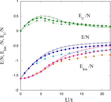
Figure 1: Ground-state energy $E/N$, kinetic energy $E_{kin}/N$ and the Coulomb energy $E_{U}/N$ for $\psi_{\lambda}$ as a function of $U$ on a $10\times 10$ lattice. We use $N_{e}=88$ and $t^{\prime}=0$ with the periodic boundary condition in one direction and antiperiodic one in the other direction. The expectation values for the Gutzwiller function are also shown by open circles. The results $E/N$, $E_{kin}/N$ and $E_{U}/N$ for $N_{e}=80$ evaluated by $\psi_{\lambda}$ are also shown by dashed lines.

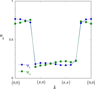
Figure 2: Momentum distribution function $n_{k}$ for $N_{e}=88$ and $U=10t$ on a $10\times 10$ lattice. The results for $\psi_{\lambda}$ (circles) and $\psi_{G}$ (squares) are shown.

IV Kinetic energy enhancement of superconductivity

IV.1 Why does the Gutzwiller-BCS state become stable?

In the original BCS theory, the superconducting condensation energy comes from the attractive potential interaction. Let us examine the reason why the Gutzwiller-BCS state $P_{G}\psi_{BCS}$ becomes stable in the presence of the on-site Coulomb repulsive interaction. We show the kinetic energy $E_{kin}$ and the Coulomb energy $E_{U}$ in Fig. 3 and Fig. 4 for $P_{G}\psi_{BCS}$, respectively. The Coulomb energy decreases as $\Delta_{sc}$ increases and at the same time the kinetic energy increases. The total ground energy $E$ has a minimum as shown in Fig. 5. We can say that the Gutzwiller-BCS state belongs to the same class of superconductivity in the sense that superconductivity is induced by the potential energy. This shows that the Gutzwiller-BCS state $\psi_{G-BCS}=P_{G}\psi_{BCS}$ is stabilized due to the reduction of the Coulomb potential energy in a similar way to the BCS state, indicating that the Gutzwiller-BCS superconductivity is a potential energy driven superconductivity.

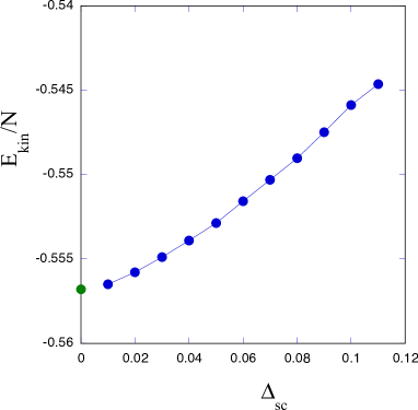
Figure 3: Kinetic energy $E_{kin}/N$ for the Gutzwiller function as a function of the gap function $\Delta_{sc}$ for $U=18$ and $N_{e}=88$ on a $10\times 10$ lattice. The extrapolated value for $\Delta_{sc}\rightarrow 0$ is shown on the y-axis.

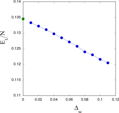
Figure 4: Coulomb energy $E_{U}/N$ for the Gutzwiller function as a function of the gap function $\Delta_{sc}$ for $U=18$ and $N_{e}=88$ on a $10\times 10$ lattice. The extrapolated value for $\Delta_{sc}\rightarrow 0$ is shown on the y-axis.

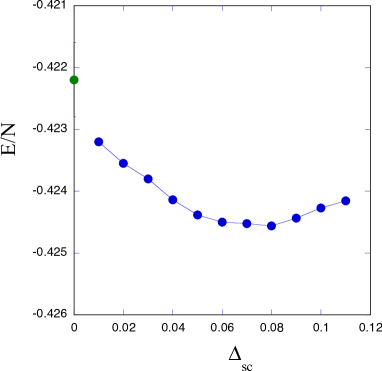
Figure 5: Ground-state energy $E/N$ for the Gutzwiller function as a function of the gap function $\Delta_{sc}$ for $U=18$ and $N_{e}=88$ on a $10\times 10$ lattice. The circle on the y-axis denotes the value extrapolated from $E_{kin}$ and $E_{U}$ for $\Delta_{sc}\rightarrow 0$.

IV.2 Why is the SC condensation energy so small?

The $U$-part of the condensation energy $\Delta E_{U-sc}$ is clearly proportional to $U$. Then $\Delta E_{U-sc}$ ca be large when $U$ is large and we can expect high-temperature superconductivity. The SC condensation energy $\Delta E_{sc}$ is, however, very small compared to the transfer $t$. $\Delta E_{sc}$ becomes very small due to the offset of $\Delta E_{kin-sc}$ and $\Delta E_{U-sc}$. As a result the SC transition temperature $T_{c}$ is very much lower than we expect. We can say that $\Delta E_{sc}$ is determined by the competition between kinetic energy effect and interaction effect. Two competitions occur where one is the competition between superconductivity and antiferromagnetism and then the other occurs between kinetic energy and interaction energy. The superconducting transition occurs as a result of two competitions.

IV.3 How does the $\psi_{\lambda-BCS}$ state become stable?

We turn to the improved off-diagonal function $\psi_{\lambda}$. We estimate the kinetic energy in the superconducting state $\psi_{\lambda-BCS}$yan21 . We define the SC condensation energy $\Delta E_{sc}$ as a sum of two contributions $\Delta E_{kin-sc}$ and $\Delta E_{U-sc}$:

$$\Delta E_{sc} = E(\Delta=0)-E(\Delta=\Delta_{{\rm opt}}),$$ (11)

$$\Delta E_{kin-sc} = E_{kin}(\Delta=0)-E_{kin}(\Delta=\Delta_{{\rm opt}}),$$ (12)

$$\Delta E_{U-sc} = E_{U}(\Delta=0)-E_{U}(\Delta=\Delta_{{\rm opt}}),$$ (13)

where $\Delta=\Delta_{sc}$ is the SC order parameter and $\Delta_{{\rm opt}}$ is the optimized value which gives the energy minimum. We have

$$\Delta E_{sc}=\Delta E_{kin-sc}+\Delta E_{U-sc}.$$ (14)

The kinetic energy in $\psi_{\lambda-BCS}$ is lower than the kinetic energy in the normal state $\psi_{\lambda}$, which is shown in Fig. 6. The Coulomb energy expectation value increases as $\Delta_{sc}$ increases as shown in Fig. 7. The results show

$$\Delta E_{kin-sc}>0,~{}~{}~{}~{}\Delta E_{U-sc}<0,$$ (15)

for $\psi_{\lambda-BCS}$ with $U=18t$ and the hole density $x=0.12$. Then the ground state becomes superconducting as shown in Fig. 8 where the ground state energy $E$ is shown as a function of $\Delta_{sc}$. This is in contrast to the Gutzwiller-BCS state and original BCS state for which $\Delta E_{kin-sc}<0$ and $\Delta E_{U-sc}>0$. We summarize this in Table. 1.

Table 1: Variations of the kinetic and potential energies in the superconducting state compared to the normal state. $T$ and $V$ denote the kinetic energy and potential energy, respectively.

State	T	V
BCS	$\Delta T>0$	$\Delta V<0$	weak coupling SC
Gutzwiller-BCS	$\Delta T>0$	$\Delta V<0$	weakly correlated SC
$\lambda$-BCS	$\Delta T<0$	$\Delta V>0$	strongly correlated SC

IV.4 Kinetic energy enhancement of superconductivity

We define the difference of the kinetic energy as

$$\Delta E_{kin}=E_{kin}(\psi_{G})-E_{kin}(\psi_{\lambda}),$$ (16)

where $E_{kin}(\psi_{G})$ and $E_{kin}(\psi_{\lambda})$ indicate the kinetic energy for $\psi_{G}$ and $\psi_{\lambda}$, We can write $\Delta E_{kin}=E_{kin}(\lambda=0)-E_{kin}(\lambda)$ for the optimized value of $\lambda$. $\Delta E_{kin}$ has the close relation with the SC condensation energy $\Delta E_{sc}$ and its kinetic part $\Delta E_{kin-sc}$.

We show $\Delta E_{kin}/N$ in Fig. 9 for $x=0.12$ where $x$ is the hole doping rate. The Coulomb energy $E_{U}/N$ and the superconducting condensation energy $\Delta E_{sc}/N$ are also shown in Fig. 9. $\Delta E_{kin}$ begins to increase after the Coulomb energy $E_{U}$ reaches the peak when $U\approx 8t$. The y axis on the right shows $\Delta E_{kin-sc}/N$ in Fig. 9. $\Delta E_{kin-sc}$ shows a similar behavior to $\Delta E_{kin}$. $\Delta E_{kin-sc}$ may change sign as a function of $U$, which is consistent with the analysis for Bi₂Sr₂CaCu₂O_8+δdeu06 . This shows the kinetic energy enhancement of superconductivity.

We compare the kinetic energy difference $\Delta E_{kin}/N$ for $x=0.12$ (the electron density $n=0.88$) and $x=0.20$ ($n=0.80$) in Fig. 10. $\Delta E_{kin}/N$ decreases when the hole density increases.

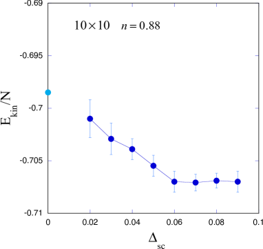
Figure 6: Kinetic energy $E_{kin}/N$ for $\psi_{\lambda-BCS}$ as a function of the gap function $\Delta_{sc}$ for $U=18$ and $N_{e}=88$ on a $10\times 10$ lattice. The circle for $\Delta_{sc}=0$ denotes the extrapolated value.

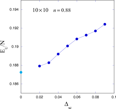
Figure 7: Coulomb energy $E_{U}/N$ for $\psi_{\lambda-BCS}$ as a function of the gap function $\Delta_{sc}$ for $U=18$ and $N_{e}=88$ on a $10\times 10$ lattice. The circle for $\Delta_{sc}=0$ denotes the extrapolated value.

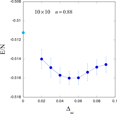
Figure 8: Ground-state energy $E/N$ for $\psi_{\lambda-BCS}$ as a function of the gap function $\Delta_{sc}$ for $U=18$ and $N_{e}=88$ on a $10\times 10$ lattice. The circle for $\Delta_{sc}=0$ denotes the extrapolated value which agrees with the value obtained by evaluations for the normal state wave function within statistical error.

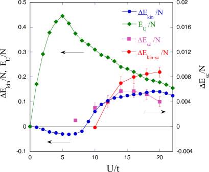
Figure 9: Kinetic-energy difference $\Delta E_{kin}/N$ and the kinetic-energy gain $\Delta E_{kin-sc}/N$ in the superconducting state $\psi_{\lambda-BCS}$ as a function of $U$ on a $10\times 10$ lattice where $N_{e}=88$ and $t^{\prime}=0$. The Coulomb energy $E_{U}/N$ for $\psi_{\lambda}$ and the condensation energy $\Delta E_{SC}$ are also shown. We use the same periodic and antiperiodic boundary conditions as in Fig. 1. The y axis on the right shows the superconducting condensation energy $\Delta E_{sc}$ and the kinetic condensation energy $\Delta E_{kin-sc}/N$ for $\psi_{\lambda}$.

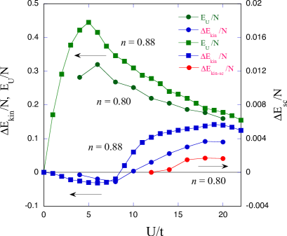
Figure 10: The Coulomb energy $E_{U}/N$, Kinetic-energy difference $\Delta E_{kin}/N$ and the kinetic-energy gain $\Delta E_{kin-sc}/N$ as a function of $U$ on a $10\times 10$ lattice where $N_{e}=80$ ($n=0.80$). $\Delta E_{kin}/N$ and $E_{U}/N$ for $n=0.88$ are also shown for comparison. We use the same boundary conditions as in Fig. 1.

V Summary

We have investigated the electronic properties of the two-dimensional Hubbard model by using the wave function with $e^{-\lambda K}$ correlation operator. The operator $e^{-\lambda K}$ plays a role that is similar to the renormalization group method. $e^{-\lambda K}$ suppresses high-energy modes and would project out low lying modes near the Fermi surface. This is typically shown in the behavior of momentum distribution function $n_{{\bf k}}$.

We examined the kinetic energy effect in SC states. The Gutzwiller-BCS state is the potential energy driven SC state, because the SC condensation energy comes from the Coulomb interaction energy. This is the same as the original BCS state where the superconductivity appears due to the attractive interaction. We evaluated the kinetic energy in the improved SC state ($\psi_{\lambda-BCS}$) to find that the kinetic energy gain stabilizes SC state while the expectation value of Coulomb interaction energy increases. This indicates that superconductivity is enhanced due to the kinetic energy effect.

The kinetic energy difference $\Delta E_{kin}=E_{kin}(\psi_{G})-E_{kin}(\psi_{\lambda})$ changes sign at $U/t\sim 9$ and increases for $U>10t$. $\Delta E_{kin-sc}$ in the SC state behaves like $\Delta E_{kin}$ for $U>10t$, showing a correlation between $\Delta E_{kin-sc}$ and $\Delta E_{kin}$. This indicates the kinetic energy enhancement of superconductivity in the strongly correlated phase. The kinetic energy enhanced mechanism of superconductivity may be different from the conventional mechanism of weak coupling superconductivity.

We here give a discussion on recent results by quantum Monte Carlo methodqin20 , where the ground state of the 2D Hubbard model is investigated for $U=8$ and the hole density $x=1/8$. An antiferromagnetic correlation is large and the uniform SC state is not stable for this set of parameters. We should examine the large-$U$ case where $U$ is greater than the bandwidth so that an antiferromagnetic correlation is suppressed. The striped state may be realized just at $x=1/8$. In the striped state the paired holes mainly exist along stripes. An inhomogeneous SC state will be realized and a pair correlation function may be anisotropic.

We lastly discuss on the improvement of the wave function. The importance of the exponential factor $e^{-\lambda K}$ is clear it is of course necessary to improve the wave function further by multiplying $P_{G}$ and $e^{-\lambda K}$ again. The improved wave function is written as $\psi_{m}=e^{-\lambda_{m}K}P_{G}\cdots e^{-\lambda_{1}K}P_{G}\psi_{0}$. $\psi_{m}$ approaches the exact ground-state wave function as $m$ increases. We believe that we obtain qualitatively the same result for further improved functions because we obtained the finite SC condensation energy in the limit $m\rightarrow\infty$yan99 .

A part of computations was supported by the Supercomputer Center of the Institute for Solid State Physics, the University of Tokyo and the Supercomputer system Yukawa-21 of the Yukawa Institute for Theoretical Physics, Kyoto University. This work was supported by a Grant-in-Aid for Scientific Research from the Ministry of Education, Culture, Sports, Science and Technology of Japan (Grant No. 17K05559).

References

- (1) J. B. Bednorz, K. A. Müller: Z. Phys. B 64, 189 (1986).
- (2) K. McElroy et al.: Nature 422, 592 (2003).
- (3) N. E. Hussey et al.: Nature 425, 814 (2003).
- (4) C. Weber, K. Haule, G. Kotliar: Phys. Rev. B 78, 134519 (2008).
- (5) M. S. Hybertsen, M. Schlüter, N. E. Christensen: Phys. Rev. B 39, 9028 (1989).
- (6) H. Eskes, G. A. Sawatzky, L. F. Feiner: Physica C 160, 424 (1989).
- (7) A. K. McMahan, J. F. Annett, R. M. Martin: Phys. Rev. B 42, 6268 (1990).
- (8) H. Eskes, G. Sawatzky: Phys. Rev. B 43, 119 (1991).
- (9) V. J. Emery: Phys. Rev. Lett. 58, 2794 (1987).
- (10) J. E. Hirsch, E. Y. Loh, D. J. Scalapino, S. Tang: Phys. Rev. B 39, 243 (1989).
- (11) R. T. Scalettar, D. J. Scalapino, R. L. Sugar, S. R. White: Phys. Rev. B 44, 770 (1991).
- (12) A. Oguri, T. Asahata, S. Maekawa: Phys. Rev. B 49, 6880 (1994).
- (13) S. Koikegami, K. Yamada: J. Phys. Soc. Jpn. 69, 768 (2000).
- (14) T. Yanagisawa, S. Koike, K. Yamaji: Phys. Rev. B 64, 184509 (2001),
- (15) T. Yanagisawa, S. Koike, K. Yamaji: Phys. Rev. B 67, 132408 (2003).
- (16) T. Yanagisawa, M. Miyazaki, K. Yamaji: J. Phys. Soc. 78, 031706 (2009).
- (17) C. Weber, A. Lauchi, F. Mila, T. Giamarchi: Phys. Rev. Lett. 102, 017005 (2009).
- (18) B. Lau, M. Berciu, G. A. Sawatzky: Phys. Rev. Lett. 106, 036401 (2011).
- (19) C. Weber, T. Giamarchi, C. M. Varma: Phys. Rev. Lett. 112, 117001 (2014).
- (20) A. Avella, F. Mancini, F. Paolo, E. Plekhano: Euro. Phys. J. B 86, 265 (2013).
- (21) H. Ebrahimnejad, G. A. Sawatzky, M. Berciu: J. Phys. Cond. Matter 28, 105603 (2016).
- (22) S. Tamura, H. Yokoyama: Phys. Procedia 81, 5 (2016).
- (23) J. Hubbard: Proc. Roy. Soc. London 276, 238 (1963).
- (24) J. Hubbard: Proc. Roy. Soc. London 281, 401 (1964).
- (25) M. C. Gutzwiller: Phys. Rev. Lett. 10, 159 (1963).
- (26) S. Zhang, J. Carlson, J. E. Gubernatis: Phys. Rev. B 55, 7464 (1997).
- (27) S. Zhang, J. Carlson, J. E. Gubernatis:. Phys. Rev. Lett. 78, 4486 (1997).
- (28) T. Yanagisawa, Y. Shimoi, K. Yamaji: Phys. Rev. B 52, R3860 (1995).
- (29) T. Nakanishi, K. Yamaji, T. Yanagisawa: J. Phys. Soc. Jpn. 66, 294 (1997).
- (30) K. Yamaji, T. Yanagisawa, T. Nakanishi, S. Koike: Physica C 304, 225 (1998).
- (31) S. Koike, K. Yamaji, T. Yanagisawa: J. Phys. Soc. Jpn. 68, 1657 (1999).
- (32) K. Yamaji, T. Yanagisawa, M. Miyazaki, R. Kadono: J. Phys. Soc. Jpn. 80, 083702 (2011).
- (33) T. M. Hardy, P. Hague, J. H. Samson, A. S. Alexandrov: Phys. Rev. B 79, 212501 (2009).
- (34) T. Yanagisawa, M. Miyazaki, K. Yamaji: J. Mod. Phys. 4, 33 (2013).
- (35) N. Bulut: Advances in Phys. 51, 1587 (2002).
- (36) H. Yokoyama, Y. Tanaka, M. Ogata, H. Tsuchiura: J. Phys. Soc. Jpn. 73, 1119 (2004).
- (37) H. Yokoyama, M. Ogata, Y. Tanaka: J. Phys. Soc. Jpn. 75, 114706 (2006).
- (38) T. Aimi, M. Imada: J. Phys. Soc. Jpn. 76, 113708 (2007).
- (39) M. Miyazaki, T. Yanagisawa, K. Yamaji: J. Phys. Cehm. Solids 63, 1403 (2002).
- (40) T. Yanagisawa: New J. Phys. 10, 023014 (2008).
- (41) T. Yanagisawa: New J. Phys. 15, 033012 (2013).
- (42) T. Yanagisawa: J. Phys. Soc. Jpn. 85, 114707 (2016).
- (43) T. Yanagisawa: J. Phys. Soc. Jpn. 88, 054702 (2019).
- (44) T. Yanagisawa: Condens. Matter 4, 57 (2019).
- (45) N. F. Mott: Metal-Insulator Transitions 1974, Taylor and Francis Ltd, London.
- (46) J. M. Tranquada, J. D. Axe, N. Ichikawa, Y. Nakamura, S. Uchida, B. Nachumi: Phys. Rev. B 54, 7489 (1996).
- (47) T. Suzuki, T. Goto, K. Chiba, T. Shinoda, T. Fukase, H. Kimura, K. Yamada, M. Ohashi, Y. Yamaguchi: Phys. Rev. B 57, R3229 (1998).
- (48) K. Yamada, C. H. Lee, K. Kurahashi, J. Wada, S. Wakimoto, S. Ueki, H. Kimura, Y. Endoh, S. Hosoya, G. Shirage, J. Birgeneau, M. Greven, M. A. Kastner, Y. J. Kim: Phys. Rev. B 57, 6165 (1998).
- (49) M. Arai, T. Nishijima, Y. Endoh, T. Egami, S. Tajima, K. Tomimoto, Y. Shiohara, M. Takahashi, A. Garrett, S. M. Benningtonn: Phys. Rev. Lett. 83, 608 (1999).
- (50) H. A. Mook, P. Dai, F. Doga, R. D. Hunt: Nature 404, 729 (2000).
- (51) S. Wakimoto, R. J. Birgeneau, M. A. Kastner, Y. S. Lee, R. Erwin, P. M. Gehring, S. H. Lee, M. Fujita, K. Yamada, Y. Edoh, K. Hirota, G. Shirane: Phys. Rev. B 61, 3699 (2000).
- (52) A. Bianconi, N. L. Saini, A. Lanzara, M. Missori, T. Rossetti, H. Oyaagi, H. Yamaguchi, K. Oka, T. Ito: Phys. Rev. Lett. 76, 3412 (1996).
- (53) T. A. Maier, G. Alvarez, M. Summers and T. C. Schulthess: Phys. Rev. Lett. 104, 247001 (2010).
- (54) R. Mondaini, T. Ying, T. Paiva and R. T. Scalettar, Phys. Rev. B86, 184506 (2012).
- (55) A. Bianconi: Nature Phys. 9, 536 (2013).
- (56) J. E. Hoffman, K. McElroy, D.-H. Lee, K. M. Lang, H. Eisaki, S. Uchida, J. C. Davis: Science 295, 466 (2002).
- (57) W. D. Wise, M. C. Boyer, K. Chatterjee, T. Kondo, T. Takeuchi, H. Ikuta, Y. Wang, E. W. Hudson: Nature Phys. 4, 696 (2008).
- (58) T. Hanaguri, C. Lupien, Y. Kohsaka, D.-H. Lee, M. Azuma, M. Takano, H. Takagi, J. C. Davis: Nature 430, 1001 (2004).
- (59) T. Yanagisawa, S. Koike, M. Miyazaki, K. Yamaji: J. Phys. Condens. Matter 14, 21 (2001).
- (60) T. Ying, R. Mondaini, X. D. Sun, T. Paiva, R. M. Fye and R. T. Scalettar, Phys. Rev. B 90, 075121 (2014).
- (61) S. Yang, T. Ying, W. Li, J. Yang, X. Sun and X. Li, J. Phys. Condens. Matter 33, 115601 (2021).
- (62) T. Yanagisawa, S. Koike, K. Yamaji: J. Phys. Soc. Jpn. 67, 3867 (1998).
- (63) T. Yanagisawa, M. Miyazaki: EPL 107, 27004 (2014).
- (64) Th. A. Maier, M. Jarrell, A. Macridin, C. Slezak: Phys. Rev. Lett. 92, 027005 (2004).
- (65) M. Ogata, H. Yokoyama, Y. Yanase, Y. Tanaka, H. Tsuchiura: J. Phys. Chem. Solids 67, 37 (2006).
- (66) E. Gull, A. J. Millis: Phys. Rev. B 86, 241106 (2012).
- (67) L. F. Tocchio, F. Becca, S. Sorella: Phys. Rev. B 94, 195126 (2016).
- (68) S. Feng: Phys. Rev. B 68, 184501 (2003).
- (69) P. Wrobel, R. Eder, R. Micnas: J. Phys.: Condens. Matter 15, 2755 (2003).
- (70) H. Guo, S. Feng: Phys. Lett. A 361, 382 (2007).
- (71) H. Otsuka: J. Phys. Soc. Jpn. 61, 1645 (1992).
- (72) T. Yanagisawa, S. Koike, K. Yamaji: J. Phys. Soc. Jpn. 68, 3608 (1999).
- (73) D. Eichenberger, D. Baeriswyl: Phys. Rev. B 76, 180504 (2007).
- (74) D. Baeriswyl, D. Eichenberger, M. Menteshashvii: New J. Phys. 11, 075010 (2009).
- (75) D. Baeriswyl: J. Supercond. Novel Magn. 24, 1157i (2011).
- (76) T. Yanagisawa: Phys. Rev. B 75, 224503 (2007).
- (77) P. W. Anderson, Science 235, 1196 (1987).
- (78) K. G. Wilson: Rev. Mod. Phys. 47, 773 (1975).
- (79) T. Yanagisawa, M. Miyazaki, K. Yamaji: Proceeding of International Conference on Quantum Complex Matter 2020; Condensed Matter 6, 12 (2021).
- (80) G. Deutscher, A. F. Santander-Syro, N. Bontemps: Phys. Rev. B 72, 092504 (2005).
- (81) M. Qin, C.-M. Chung, H. Shi, E. Vitali, C. Hubig, U. Schollwöck, S. R. White and S. Zhang, Phys. Rev. X 10, 031016 (2020).