Universality and Optimality of Structured Deep Kernel Networks

Abstract

Kernel based methods yield approximation models that are flexible, efficient and powerful. In particular, they utilize fixed feature maps of the data, being often associated to strong analytical results that prove their accuracy. On the other hand, the recent success of machine learning methods has been driven by deep neural networks (NNs). They achieve a significant accuracy on very high-dimensional data, in that they are able to learn also efficient data representations or data-based feature maps.

In this paper, we leverage a recent deep kernel representer theorem to connect the two approaches and understand their interplay. In particular, we show that the use of special types of kernels yield models reminiscent of neural networks that are founded in the same theoretical framework of classical kernel methods, while enjoying many computational properties of deep neural networks. Especially the introduced Structured Deep Kernel Networks (SDKNs) can be viewed as neural networks with optimizable activation functions obeying a representer theorem.
Analytic properties show their universal approximation properties in different asymptotic regimes of unbounded number of centers, width and depth. Especially in the case of unbounded depth, the constructions is asymptotically better than corresponding constructions for ReLU neural networks, which is made possible by the flexibility of kernel approximation.

Keywords Kernel methods $\cdot$ Neural networks $\cdot$ Deep learning $\cdot$ Representer theorem $\cdot$ Universal approximation

1 Introduction

In the framework of data based simulation and engineering, high-dimensional scattered data approximation and machine learning techniques are of utmost importance [30]. They construct purely data-based models which can capture the input-output behavior of complex systems through the knowledge of a finite number of measurements. For a successful application in this context, machine learning methods are required to work with high dimensional scattered data to produce models that are efficient and reliable.
One machine learning technique that satisfies these specifications are given by kernel based methods [36]. They are centered around the concept of positive definite kernels and their associated Reproducing Kernel Hilbert Space (RKHS), which provides a rich and unified theoretical framework for their analysis due to a representer theorem [16, 32]. Kernel-based algorithms can be understood as the application of a simple, linear algorithm on the input data transformed by means of a fixed non-linear and possibly infinite-dimensional feature map, which associates the input value to an element of a high (or infinite) dimensional Hilbert space. These feature maps can be either implicitly represented by the chosen kernel, or be manually designed to embed relevant structures of the data, including non Euclidean ones.
Another approach which gained more popularity in the recent years due to increased computational power and unprecendented availability of large data sets is given by deep neural networks [11]. These methods manage to reach an unprecedented accuracy on very high dimensional problems, but are based on completly different premises: Based on a multilayer setup, composed of linear mappings and nonlinear activation functions, they also learn a feature representation of the data themself instead of using a fixed feature map.

It is thus particularly natural and promising to investigate multilayer kernel approximants obtained by composition of several kernel-based functions. Although this approach has been already pursued in some direction, a recent result has laid the foundations of a new analysis through the establishment of a representer theorem for multilayer kernels [2]. Still, the actual solution of the learning problem presents several challenges both on a computational and on a theoretical level. First, despite one can move from infinite to finite dimensional optimization via the representer theorem, the problem is non-convex and still very hard to solve numerically. Second, the rich theoretical foundation of the shallow (single-layer) case can not be directly transferred to this situation.

In this view, in this paper we start by analyzing possible ways of using the deep representer theorem and highlight some limitations of a straightforward approach (Section 3.1). We then use our insights to introduce a suitable architecture (i.e., a specification of the choice of the kernels and of their composition into multiple layers) that makes the solution of the optimization problem possible with efficient methods. More precisely, we construct two basic layers, one that is using the linear kernel, and one that is built by means of a nonlinear kernel applied componentwise (Section 3.2). We use these layers as building blocks that can be stacked into a Structured Deep Kernel Network (SDKN), whose architecture is reminiscent of feedforward neural networks. We comment on the optimality and the relation to a deep neural network representer theorem (Section 3.3). In Section 4 we show the full flexibility of the new family of SDKNs by proving universal approximation properties and elucidating improved constructions which are made possible by using kernel mappings.

To keep the presentation easy to follow, we do not include experimental results with those SDKN in the present article. But we refer to [37] for an example of a successful application and comparison of the SDKN to NN in the context of closure term prediction for computational fluid dynamics. We also have positive experience with the SDKN architecture in various other application settings such as spine modelling and frameworks such as kernel autoencoders which are subject of ongoing work.

2 Kernel methods and neural networks

We start by recollecting some background material that is required for the following discussion.
We consider an input domain $\Omega\subset\mathbb{R}^{d_{0}}$ and a target domain $Y\subset\mathbb{R}^{{d_{out}}}$ as well as a scatttered data set $D=((x_{1},y_{1}),..,(x_{N},y_{N}))$. In the context of statistical learning theory, this data set is assumed to be distributed according to a typically unknown probability distribution $\mathcal{P}$, i.e. $(X_{N},Y_{N})\sim\mathcal{P}^{N}$. The values $y_{i}$ can be distributed according to some target function $g$, possibly affected by noise.Formally, approximating this data means minimizing a loss over a suitable space $\mathcal{H}$ of functions, for example by

$$f^{*}:=\operatorname*{arg\min}_{f\in\mathcal{H}}\mathcal{L}_{D}(f),\quad\mathcal{L}_{D}(f):=\frac{1}{N}\sum_{i=1}^{N}L(x_{i},y_{i},f(x_{i})).$$ (1)

Depending on the structure of $\mathcal{H}$, it might be required to extend the loss by a regularization term, in order to improve the generalization of the function $f^{*}$ also to unseen data. This corresponds to minimizing a cost function $\mathcal{J}$ that consist of both loss and regularization, i.e. $\mathcal{J}(f):=\mathcal{L}_{D}(f)+\mathcal{R}(f)$. However there are also other approaches to archieve good generalization, without using an explicit regularization term $\mathcal{R}$ [11].

In the case of absence of noise, the goal is simply to approximate the function $g$, which will be done in the following using the supremum norm $\|g\|_{\infty}:=\sup_{x\in\Omega}\left\|g(x)\right\|_{2}$. For this it is important that the machine learning approach describes a sufficiently large set of functions. This will be discussed in Section 2.3. Before, kernel methods and neural networks are introduced in Section 2.1 and Section 2.2. Section 2.4 recalls the deep kernel representer theorem and finally Section 2.5 provides an overview on related work.

2.1 Approximation with kernel methods

Kernel methods are a popular and successful family of algorithms in machine learning and approximation theory, and they may be used to address this approximation task. We point the reader to [36, 9] for more background information. They are based on the use of a positive definite kernel, i.e., a symmetric function $k:\Omega\times\Omega\to\mathbb{R}$ such that the kernel matrix $(k(x_{i},x_{j}))_{i,j=1}^{N}\in\mathbb{R}^{N\times N}$ is positive semi-definite for any set of $N$ points $X_{N}\subset\Omega$, $N\in\mathbb{N}$. If the matrix is even positive definite whenever the points are pairwise distinct, the kernel is denoted strictly positive definite. Given a strictly positive definite kernel $k$ on a domain $\Omega$, there exists a unique reproducing kernel Hilbert space (RKHS).

Radial Basis Functions (RBFs) are a notable class of kernels that are defined as $k(x,y):=\varphi(\varepsilon\|x-y\|_{2})$ with a width (or shape parameter) $\varepsilon>0$ and a univariate function $\varphi:[0,\infty)\to\mathbb{R}$. Some examples of RBFs that will be used in this work are given in Table 1.

	$\varphi(r)$
Gaussian	$\exp(-r^{2})$
Matérn of order $0$	$\exp(-r)$
Wendland of order $0$	$(1-r)_{+}:=\max(1-r,0)$

Table 1: Examples of radial basis functions $\varphi$ which yield strictly positive definite kernels $k$ on $\Omega=\mathbb{R}$.

A milestone result in kernel theory is the representer theorem (see [16, 32]). It ensures that if the loss optimization (1) over the RKHS $\mathcal{H}=\mathcal{H}_{k}(\Omega)$ has a solution, then there exists a minimizer $s$ that is actually an element of $V(X_{N}):=\operatorname*{span}\{k(\cdot,x),~{}x\in X_{N}\}\subset\mathcal{H}_{k}(\Omega)$, i.e.,

$$f(x):=\sum_{i=1}^{N}\alpha_{i}k(x,x_{i}).$$ (2)

This representer theorem also allows for the use of a regularization term that depends monotonically on the RKHS norm of the function, i.e. $\mathcal{R}(f)=\Lambda(\|f\|_{\mathcal{H}_{k}(\Omega)}^{2})$. If the function $\Lambda:\mathbb{R}_{\geq 0}\rightarrow\mathbb{R}_{\geq 0}$ is even strictly monotonically increasing, every minimizer admits to such a representation. If also convexity of both the loss function $L$ and the regularization function $\Lambda$ is assumed, there is a unique solution of this form. The infinite-dimensional optimization problem is thus reduced to a finite dimensional one.

It can be shown that for each positive definite kernel $k$ there exists at least a feature map $\phi:\Omega\rightarrow\mathcal{H}$ into a feature space $\mathcal{H}$ such that $k(x,y)=\langle\phi(x),\phi(y)\rangle_{\mathcal{H}}$. Also the opposite holds, i.e., any function $\tilde{k}(x,y):=\langle\phi(x),\phi(y)\rangle_{\mathcal{H}}$ is in fact a positive definite kernel on $\Omega$. Especially, it can be shown that kernel (ridge) regression is in fact linear regression applied to the data set $\left\{\left(\varphi(x_{i}),y_{i}\right)\right\}_{i=1}^{N}$ [11], i.e., a simple algorithm is applied to the inputs that are transformed by means of the fixed feature map. This is partly a drawback of kernel methods, as they are limited by the fact that no data representation is learned from the data themselves, as instead is the case for neural networks, as we will discuss in the next section. Using our new method this limitation is removed.

Another drawback since the rise of deep learning is that kernel methods have been considered to be less apt to process very large datasets, and indeed several limitations exists when using traditional techniques. Nevertheless, recent research has developed methods that allow a very efficient computational scalability of kernel methods. We refer for example to the Nystrom method [38], to Random Fourier Features [29], to EigenPro [21, 22] and to Falkon [23]. The last paper in particular includes also a very recent survey of state-of-the-art methods that allow to train kernel models with up to billions of points.

2.2 Approximation with neural networks

Neural network approaches are another popular and well known machine learning technique, especially due to their successful application in real world tasks such as image recognition or machine translation. In their simplest form, standard feedforward neural networks are given by a concatenation of simple functions as

$$f(x,\Theta)=W_{L}\sigma(..(\sigma(W_{2}\sigma(W_{1}x+b_{1})+b_{2})))+b_{L}$$ (3)

with weight matrices $W_{i}\in\mathbb{R}^{d_{i}\times d_{i-1}},i=1,..,L$ and bias terms $b_{i},i=1,..,L$ of suitable sizes and nonlinear activation functions $\sigma:\mathbb{R}\rightarrow\mathbb{R}$, that are applied dimensionwise. A common activation function is the ReLU function, which is given as $\sigma(x)=\max(x,0)$. Due to this multilayer structure, neural networks can easily cope with high dimensional data sets, simply by increasing the network size: Both the number of layers $L$ as well as the width determined by the inner dimensions $d_{1},..,d_{L-1}$ can be increased.
Learning such a neural networks means optimizing its parameters $\Theta:=\{W_{i},b_{i},i=1,..,L\}$ such that the loss in Eq. (1) is minimized. As the loss landscape in the parameters $\Theta$ is usually highly nontrivial, no direct optimization is feasible. Instead one usually relies on variants of stochastic gradient descent for its minimization with randomly initialized weights.
A lot of research has proved their practical success as well as the theoretical foundations: Universal approximation properties (see also Section 2.3) have been proven, the initialization of parameters was investigated, sophisticated optimization methods have been devised [11] and recent works have focussed on the overparametrized case, where the number of parameters $\Theta$ considerably exceeds the number of data points $N$ [1]. Efficient frameworks like PyTorch [27] enable the use and investigation of neural networks for a broad community. Nevertheless the theory of neural networks is not that well understood in comparison to kernel methods.

In view of Eq. (3), the neural network can be viewed as a linear model after an optimizeable feature map

$$x\mapsto\sigma(..(\sigma(W_{2}\sigma(W_{1}x+b_{1})+b_{2})).$$ (4)

This is a crucial advantage for high-dimensional data sets like images, where a combined representation and model learning is required.

2.3 Universal approximation properties

A universal approximation property states that the class of functions generated from some model is dense in a considered function space, provided the setup is chosen large enough. Such a property is required in machine learning in order to deal with complex data sets: A model that does not possess a universal approximation property cannot approximate arbitrary functions in theory and can thus not be expected to learn sufficient relations within complex datasets practically.

1. For kernel methods, the question is whether functions described via Eq. (2) for $N\rightarrow\infty$ are a sufficiently rich class of functions. This question is adressed via the notion of universal kernels: A kernel is called universal, if its RKHS $\mathcal{H}_{k}(\Omega)$ is dense in the Banach space of continuous function $C(\Omega)$. As the space of so called kernel translates, i.e. $\operatorname*{span}\{k(\cdot,x),x\in\Omega\}$ is dense in the RKHS $\mathcal{H}_{k}(\Omega)$, this property directly answers the question of universal approximation. We refer to [24] for further details and remark, that common kernels like the radial basis function kernels given in Table 1 are universal kernels.

2. For standard neural networks, the question is whether the parametrization of functions via Eq. (3) is sufficiently rich. This is answered for different limit cases: For the case of wide networks (that is $d_{1},..,d_{L-1}\rightarrow\infty$) see e.g. [14, 19, 28] and for the case of deep networks (that is $L\rightarrow\infty$) see e.g. [8, 34, 13]. We remark that a lot of recent approximation results for very deep neural networks have focussed on the popular ReLU activation function.

2.4 Deep kernel representer theorem

The following deep kernel representer theorem with slightly modified notation was stated and proved in [2]. It generalizes the standard representer theorem to multilayer kernel methods with matrix-valued kernels and thus constitutes a solid theoretical foundation:

Theorem 1 (Concatenated representer theorem).

Let $\mathcal{H}_{1},..,\mathcal{H}_{L}$ be reproducing kernel Hilbert spaces of functions with finite-dimensional domains $D_{l}$ and ranges $R_{l}\subseteq\mathbb{R}^{d_{l}}$ with $d_{l}\in\mathbb{N}$ for $l=1,..,N$ such that $R_{l}\subseteq D_{l+1}$ for $l=1,..,L-1,D_{1}=\Omega$ and $R_{L}\subset\mathbb{R}$. Let furthermore $\mathcal{L}:\mathbb{R}^{2}\rightarrow[0,\infty]$ be an abitrary loss function and let $\Theta_{1},..,\Theta_{L}:[0,\infty)\rightarrow[0,\infty)$ be strictly monotonically increasing functions. Then, a minimizing tuple $(f_{l}^{*})_{l=1}^{L}$ with $f_{l}^{*}\in\mathcal{H}_{l}$ of

$$J(f_{1},..,f_{L}):=\sum_{i=1}^{N}\mathcal{L}(y_{i},f_{L}\circ..\circ f_{1}(x_{i}))+\sum_{l=1}^{L}\Theta_{l}(\|f_{l}\|_{\mathcal{H}_{l}^{2}}) \star$$ ()

fulfills $f_{l}^{*}\in\tilde{V}\subset\mathcal{H}_{l}$ for all $l=1,..,L$ with

$$\tilde{V}_{l}:=\operatorname*{span}\{K_{l}(~{}\cdot~{},f_{l-1}^{*}\circ..\circ f_{1}^{*}(x_{i}))e_{k_{l}}|i=1,..,N,k_{l}=1,..,d_{l}\},$$

where $K_{l}$ denotes the reproducing kernel of $\mathcal{H}_{l}$ and $e_{k_{l}}\in\mathbb{R}^{d_{l}}$ is the $k_{l}$-th unit vector.

Figure 1: Visualization of the mappings within Theorem 1.

Note that the theorem can easily be generalized to vector-valued outputs. Using this theorem, the infinite dimensional optimization problem with $f_{l}\in\mathcal{H}_{l},l=1,..,L$ boils down to a finite dimensional problem of optimizing the expansion coefficients $\alpha_{i}\in\mathbb{R}^{d_{i}}$ of

$$\tilde{V}_{l}\ni f_{l}^{*} =\sum_{i=1}^{N}K_{l}(\cdot,f_{l-1}^{*}\circ..\circ f_{1}^{*}(x_{i}))\alpha_{i}$$

$$\Rightarrow f_{l}^{*}\circ..f_{1}^{*}(\cdot) =\sum_{i=1}^{N}K_{l}(f_{l-1}^{*}\circ..\circ f_{1}^{*}(\cdot),f_{l-1}^{*}\circ..\circ f_{1}^{*}(x_{i}))\alpha_{i}.$$

Like this the overall approximant is given by

$$h(x)=f_{L}^{*}(..(f_{1}^{*}(x)))$$

which can be stated as a standard kernel approximant $f^{*}(x)=\sum_{i=1}^{N}\mathcal{K}_{L}(\cdot,\tilde{x}_{i})\alpha_{i}$ using a deep kernel $\mathcal{K}^{L}$

$$\mathcal{K}^{L}(x,y) =K_{L}(f_{L-1}\circ..\circ f_{1}(x),f_{L-1}\circ..\circ f_{1}(y)).$$ (5)

with the propagated centers $\tilde{x}_{i}=f_{L-1}\circ..\circ f_{1}(x_{i})$. Note that this kernel $\mathcal{K}^{L}$ is parametrized and learned by minimizing $(\star)$.

2.4.1 Notation

In the following, we will drop the star-notation of the functions and simply use $f_{1},..,f_{L}$. Furthermore we set $F_{1}:=f_{1}$, $F_{j}:=f_{j}\circ..\circ f_{1}$ for $j\geq 2$ such that $f^{*}(x)=F_{L}(x)$. We use a superscript notation $x^{(i)}$ to refer to the $i$-th component within the standard Euclidean vector representation, and use the same notation also for the components of functions, i.e. $f_{j}^{(i)}(x)$ denotes the $i$-th component of $f_{j}(x)$. The setting of the representer theorem with the corresponding spaces is depicted in Figure 1. As we will not focus on the inner domains $D_{l}$ and ranges $R_{l}$, they are not stated explicitly, but the dimensions $d_{0},d_{1},..,d_{L}$.

2.5 Related work

In order to obtain the flexibility of feature representation learning instead of using a fixed feature map, several multilayer kernel methods have been proposed. This is done frequently based on neural networks: In [18], a neural network is used in order to directly learn a kernel function from the data. The paper [39] suggests to use a neural network to transform the data, and subsequently use a fixed kernel on top. Like this the deep neural network is used as a front-end, and both parts are optimized jointly. Another approach with similarities to neural networks is proposed in [40], which introduces a setup called Deep Spectral Kernel Learning. Here a multilayered kernel mapping is built by using random fourier feature mappings in every layer. This is essentially a neural network with fixed parameters in every second layer.
Hierarchical Gaussian kernels are introduced in [33], which are an iterated composition of Gaussian kernels. The setup has as well a structure comparable with neural networks. However the methodology does not easily extend to a broader class of kernels. From a Gaussian process point of view, [4] introduces Deep Gaussian processes, which is a hierarchical composition of Gaussian processes. In order to scale them, approximation techniques are used. Under the notion of Kernel Flows, [26] introduces a way to build a kernel step-by-step, by iteratively modyfing the transformation of the data, which is described with help of standard kernel mappings.

Arc-cosine kernels are introduced in [3], which the authors also call multilayer kernel machines, that emerge in the unbounded width limit of neural networks. Further research in this direction is conducted under the notion of the neural tangent kernel [15].
Starting from the neural network point of view, there are approaches that do not use fixed activation functions but strive for optimized activation functions. The paper [35] extends the loss functional with a specific regularization term. This allows the authors to derive a representer theorem, yielding activation functions given by nonuniform linear splines. Another approach coined Kafnets is introduced in [31]. Their structure of the network is quite similar to the setup which we will derive based on the deep kernel representer theorem. However in contrast to ours, their setup is build on prechosen center points within each layer, given e.g. by a grid that is independent of the data.
We remark, that [40, 35] draw some links to the deep kernel representer theorem, but do not make use of it. By using the deep kernel representer theorem for our SDKN, we obtain optimality of our proposed setup in contrast to other approaches like standard neural networks, that enjoy the same structure. In Section 3.3 we further comment on this and especially elaborate on the connections and differences to the neural network representer theorem of [35].

3 Structured Deep Kernel Networks

In the first Section 3.1, we comment on a straightforward application of the deep kernel representer theorem (Theorem 1) using common classes of kernels and elaborate why this approach is not powerful. Subsequently, we introduce our Structured Deep Kernel Network (SDKN) approach in Section 3.2 and comment on its optimality and relation to neural networks in Section 3.3.

3.1 Radial basis function approach

A straight-forward approach would be the use of common matrix-valued radial basis function kernels like the Gaussian, Wendland or Matérn kernels, e.g.

$$k(x,y)=k_{\text{Gauss}}\cdot I_{d}\in\mathbb{R}^{d\times d}$$

or even more general matrix-valued kernels. In preliminary numerical experiments we have seen that such an approach is not successful, as there are way too much parameters to optimize that do not obey any special structure. To reduce the number of optimizable parameters and simplify the optimization, one can pick a subset $\{z_{i}\}_{i=1}^{M}\subset\{x_{i}\}_{i=1}^{N}$ for $M\ll N$ and use them as center points, such that every mapping $f_{l}:\mathbb{R}^{d_{l}}\rightarrow R^{d_{l+1}}$ is given by

$$f_{l}(\cdot)=\sum_{i=1}^{M}k_{l}(\cdot,F_{l-1}(z_{i}))\alpha_{i}$$

with optimizable parameters $\alpha_{i}\in\mathbb{R}^{d_{l+1}}$. But even this approach is experimentally inferior to the setup of SDKNs introduced below. The theoretic reason for this is likely the choice of ansatz (trial) space:
Assume the output of the function $f_{l}$ should be slightly adjusted, s.t. for $F_{l-1}(z_{i})$ it holds

$$f_{l}(F_{l-1}(z_{i})) =y_{i}+\epsilon$$

$$\text{instead of }\hskip 28.45274ptf_{l}(F_{l-1}(z_{i})) =y_{i},$$

with $\epsilon\in\mathbb{R}^{d_{l+1}}$. But due to the potentially very bad conditioning of the kernel matrix $A\in\mathbb{R}^{Md_{l}\times Md_{l}},A_{ij}=k_{l}(F_{l-1}(z_{i}),F_{l-1}(z_{j}))$ (see e.g. [5]), this results in large changes for the parameters $\alpha_{j}$ even for small $\epsilon$. This slows down the optimization when using common stochastic gradient descent optimization strategies [21].
A remedy for this might be a change of basis, e.g. using a Lagrange or Newton basis instead of the basis of kernel translates $\{k(\cdot,z_{i}),i=1,..,M\}$ [25]. However, this is not possible in deep setups with more than two layers, as the Lagrange and Newton basis both depend on the used centers $\{z_{i}\}_{i=1}^{M}$, and these change as soon as the previous functions $f_{1},..,f_{l-1}$ change.

In order to alleviate these problems, we propose a better setup with a more subtle selection of kernels, which will be called Structured Deep Kernel Network (SDKN).

3.2 Setup of structured deep kernel network

In the following, we introduce two types of kernels, namely simple linear kernels (Section 3.2.1) as well as kernels that are acting on single dimensions (Section 3.2.2) and comment on their positive definiteness in Section 3.2.3. Subsequently in Section 3.2.4, we combine these types of kernels in an alternating way.

3.2.1 Linear kernel

The linear kernel $k_{\text{lin}}:\mathbb{R}^{d}\times\mathbb{R}^{d}\rightarrow\mathbb{R}$ is defined via $(x,y)\rightarrow\langle x,y\rangle_{\mathbb{R}^{d}}$, i.e. the standard Euclidean inner product is computed. We have the following theorem:

Proposition 2.

A linear layer without bias, i.e. a mapping $\mathbb{R}^{d}\rightarrow\mathbb{R}^{b},x\mapsto Ax$ with $A\in\mathbb{R}^{b\times d}$ can be realized as a kernel mapping

$$s:\mathbb{R}^{d}\rightarrow\mathbb{R}^{b},x\mapsto\sum_{i=1}^{M}k(x,z_{i})\alpha_{i},~{}~{}\alpha_{i}\in\mathbb{R}^{b}$$

with given centers $\{z_{i}\}_{i=1}^{M}\subset\mathbb{R}^{d}$ by using a matrix valued linear kernel

$$k(x,z)=k_{\text{lin}}(x,z)\cdot I_{d}=\langle x,z\rangle_{\mathbb{R}^{d}}\cdot I_{d}, \star_{1}$$ ()

iff the span of the center points is a superset of the row space of the matrix A.

A proof is given in the appendix, see proof of 2. We remark that 2 can also be generalized to the mapping $x\mapsto Ax+c$, $c\in\mathbb{R}^{b}$, i.e. to a linear mapping with bias. However, as we will focus on translational invariant kernels in the following, such an additional bias term has no effect.
We proceed with the following proposition, which essentially shows that any linear mapping is possible, i.e. it is not required to check that the span of the center points is a specific superset as required in 2:

Proposition 3.

Consider a mapping $g:\mathbb{R}^{d_{0}}\supset\Omega\rightarrow\{(g^{(1)}(x),..,g^{(d)}(x))^{\top}~{}|~{}x\in\Omega\}=:g(\Omega)\subset\mathbb{R}^{d},x\mapsto(g^{(1)}(x),..,g^{(d)}(x))^{\top}$ with $g^{(1)},..,g^{(d)}:\Omega\rightarrow\mathbb{R}$.
Then any linear combination

$$(g^{(1)}(x),..,g^{(d)}(x))^{\top}\mapsto\sum_{j=1}^{d}g^{(j)}(x)\cdot\beta_{j}$$

with $\beta_{j}\in\mathbb{R}^{b},j=1,..,d$ can be realized with help of a linear kernel $k$ using propagated centers $g(z_{i})\in g(\Omega)$, i.e.

$$\exists z_{1},..,z_{d}\in\Omega,\alpha_{1},..,\alpha_{d}\in\mathbb{R}^{b}~{}\forall x\in\Omega$$

$$\qquad\qquad\sum_{j=1}^{d}g^{(j)}(x)\cdot\beta_{j}=\sum_{i=1}^{d}k(g(x),g(z_{i}))\cdot\alpha_{i}$$

The proof is given in the appendix, see proof of 3. The following example illustrates the statement of the proposition:

Example 4.

Choose $d_{0}=1,d=3$ and $\Omega=[0,1]$ as well as $g^{(1)}(x)=x,g^{(2)}(x)=2x,g^{(3)}(x)=x^{2}$. Consider a training set $X_{N}\subset\Omega$ with at least three pairwise distinct points, i.e. $N\geq 3$. Then the space $\operatorname*{span}\{g(z_{i}),z_{i}\in X_{N}\}\subseteq\mathbb{R}^{d}$ spanned by the propagated data points $g(z_{i})$ is only two dimensional as $(g^{(1)}(z_{i}))_{i=1}^{N}$ and $(g^{(2)}(z_{i}))_{i=1}^{N}$ are linearly dependent. In particular, it holds $\operatorname*{span}\{g(z_{i}),z_{i}\in X_{N}\}=\operatorname*{span}\{(1,2,0)^{\top},(0,0,1)^{\top}\}$.
Thus, according to 2 it is not possible to realize arbitrary linear combinations, especially since $(2,-1,0)^{\top}\perp\operatorname*{span}\{g(z_{i}),z_{i}\in X_{N}\}$ it is not possible to realize the linear combination $(g^{(1)}(x),g^{(2)}(x),g^{(3)}(x))^{\top}\mapsto 2\cdot g^{(1)}(x)-g^{(2)}(x)$. However as $g^{(1)}(x)-g^{(2)}(x)=2x-2x=0$, this contribution does not matter at all.

3.2.2 Single-dimensional kernels

The following type of kernel $k_{s}:\mathbb{R}^{d}\times\mathbb{R}^{d}\rightarrow\mathbb{R}^{d\times d}$, that is composed of $d$ strictly positive definite kernels $k^{(1)},..,k^{(d)}$ acting on one-dimensional inputs, will be called single-dimensional kernels (the index $s$ refers to single):

$$k_{s}:\mathbb{R}^{d}\times\mathbb{R}^{d}\rightarrow\mathbb{R}^{d\times d},k_{s}(x,z)=\text{diag}(k^{(1)}(x^{(1)},z^{(1)}),..,k^{(d)}(x^{(d)},z^{(d)})) \star_{2}$$ ()

Recall that the notation $x^{(i)},z^{(i)}$ means that only the $i$-th component of the vectors $x$ respective $z$ is used. In the following, we will focus on the use of radial basis function kernels for the kernels $k^{(1)},..,k^{(d)}$.

3.2.3 Positive definiteness of the employed kernels

Both classes of kernels introduced in Section 3.2 are positive-definite kernels, but in general not strictly positive definite:

1. The linear kernel introduced in Section 3.2.1 is positive definite, as its feature map is the identity mapping, i.e. the RKHS is especially finite-dimensional.

2. The single-dimensional matrix-valued kernel $k_{s}$ is also in general only positive definite, even if the used kernels $k^{(1)},..,k^{(d)}$ are strictly positive definite. This can be observed if we use $k^{(1)}=..=k^{(d)}$: The overall kernel matrix related to single-dimensional matrix-valued kernels is the diagonal concatenation of the kernel matrices concerning the single dimensions. Zero eigenvalues can occur, if some coordinate of different points coincide: Consider two data points $x_{1}\neq x_{2}\subset\mathbb{R}^{2}$ with $x_{1}^{(1)}=x_{2}^{(1)}$, i.e. the first coordinate coincides. When the Wendland kernel of order $0$ is used as the single dimensional kernel, the resulting kernel matrix is rank deficient, e.g.

   $$X_{2}=\left\{\begin{pmatrix}1\\ -0.2\end{pmatrix},\begin{pmatrix}1\\ -0.9\end{pmatrix}\right\}\Rightarrow k_{s}(X_{2},X_{2})=\begin{pmatrix}1&1&0&0\\ 1&1&0&0\\ 0&0&1&0.3\\ 0&0&0.3&1\\ \end{pmatrix}$$

   with eigenvalues $0$, $0.7$, $1.3$, $2$.

3.2.4 Overall setup

Following the notation within the deep kernel representer theorem (Theorem 1), we seek an approximant of the form $f_{L}\circ..\circ f_{1}(\cdot)$. We will use $L$ odd and use alternately the linear kernel from Section 3.2.1 and the single-dimensional kernels from Section 3.2.2, where we always start (and therefore end) with the linear kernel. The dimensionality of the output of these matrix-valued kernels directly corresponds to the dimensionality of the inner spaces and can be chosen arbitrarily.

The overall setup is therefore depicted in Figure 2 and is reminiscent of the architecture of standard feedforward neural networks:

1. The mappings $f_{l}$ for $l$ odd use the linear kernel ($\star_{1}$) and thus can realize linear mappings $x\mapsto Ax$ via 2, especially any linear mapping that is compatible with the data in the sense of Theorem 3 can be realized.

2. The mappings $f_{l}$ for $l$ even use the single-dimensional kernels ($\star_{2}$). Thus these mappings have the following form:

   $$f_{l}^{(j)}(x)=\sum_{i=1}^{N}\alpha_{l,i}^{(j)}k_{j}(x^{(j)},F_{j-1}(z_{i})^{(j)})$$

   with $\alpha_{l,i}^{(j)}\in\mathbb{R}$. These functions $f_{l}^{(j)}$ for $l=2,4,..,\ j=1,..,d_{l}$ can be viewed as activation functions, which are also present in neural networks. However, as the parameters $\alpha_{l,i}^{(j)}$ are subject to optimization, these functions are optimizable activation functions. This is a conceptual advantage over NNs that mostly use fixed or parametrized activation functions.
   In order to enforce sparsity and allow for a quick evaluation, we only use $M\ll N$ training points (called centers) of the whole data set $X_{N}$, i.e. the remaining coefficients are set to zero at initialization and remain fixed. Thus we have

   $$f_{l}^{(j)}(x)=\sum_{i=1}^{M}\alpha_{l,i}^{(j)}k_{j}(x^{(j)},F_{j-1}(z_{i})^{(j)}).$$ (6)

   This sparsity speeds up the optimization procedure in a practical implementation and does not impede the approximation capabilites as analysed in Section 4.

Figure 2: Visualization of the overall Structured Deep Kernel Network (SDKN). Throughout the figures, gray arrows refer to layers using the linear kernel, while black arrows refer to layers using the single dimensional kernel. The braces below the layers indicate the similarities to neural networks.
The illustrated SDKN has a depth of $L=2$, a maximal dimension (width) of $w=4$ and the dimensions $d_{0}=2,d_{1}=d_{2}=d_{3}=d_{4}=4,d_{5}=2$ (see notation introduced in Section 4).

3.3 Generality, optimality and sparsity

We want to highlight some positive properties of our SDKN approach, especially that it is more general than existing results in this direction. This will in particular involve relating our approach to [35], where a representer theorem for deep neural networks is derived. In order to do so, the authors make use of a second-order total variation regularization term, which is motivated by favorable properties of activation functions: They should be simple for practical relevance and piecewise linear, because this works in practice. Thus the authors conclude that the “most favorable choice” of a search space for activation functions is given by

$$\begin{aligned} \text{BV}^{(2)}(\mathbb{R})=&\{f:\mathbb{R}\rightarrow\mathbb{R}~{}\text{s.t.}~{}\|D^{2}f\|_{\mathcal{M}}<\infty\}\\ \|D^{2}f\|_{\mathcal{M}}:=&\sup_{\varphi\in\mathcal{S}(\mathbb{R}):\|\varphi\|_{\infty}\leq 1}\langle D^{2}f,\varphi\rangle\\ \|f\|_{\text{BV}^{(2)}(\mathbb{R})}:=&\sqrt{|f(0)|^{2}+|f(1)-f(0)|^{2}}+\|D^{2}f\|_{\mathcal{M}}\\ \end{aligned}$$ (7)

whereby $D^{2}$ refers to the second derivative. Finally a representer theorem is derived [35, Theorem 4], which states roughly speaking that an optimal activation function (for node $n$ in layer $l$) is given by a piecewise linear spline of the form

$$\sigma_{n,l}(x)=b_{1,n,l}+b_{2,n,l}x+\sum_{k=1}^{K_{n,l}}a_{k,n,l}(x-\tau_{k,n,l})_{+}$$ (8)

with $K_{n,l}\leq N-2$ nodes and $b_{1,n,l},b_{2,n,l},a_{k,n,l},\tau_{k,n,l}\in\mathbb{R}$. Their representer theorem is comparable to the deep kernel representer theorem in conjunction with the setup of the SDKN:

• Guided by the assumption of simplicity and piecewise linearity, a choice of one-dimensional kernel like $k(x,y)=\max(1-|x-y|,0)+x\cdot y$ (Wendland kernel plus linear kernel) to build the single-dimensional kernels is reasonable and justified. Thus we obtain optimizable activation functions similar to Eq. (8) as a special case of our formulation.

• Generality of activation functions: Our approach does not make use of assumptions on simplicity and piecewise linearity as mentioned above. This means that our SDKN approach is optimal for a broader class of setups, which means that we retain the full choice of one-dimensional kernels to build our single-dimensional kernels.

• Optimality of propagated centers: The deep kernel representer theorem directly states the optimality of the propagated centers. This is a particular advantage compared to [31], where fixed centers are used within each layer.

• Optimality of linear layers: The neural network representer theorem of [35] only considers the optimality of the activation functions, but does not adress the optimality of the linear layers. This is done in our structured deep kernel setup, as the linear layers are inherently optimal by the choice of the linear kernel which gives rise to linear layers as elaborated in Section 3.2.1.

• Sparsity of the SDKN: It is shown in [35], that the piecewise linear spline from Eq. (8) satisfies $\|D^{2}\sigma_{n,l}\|_{\mathcal{M}}=\sum_{k=1}^{K_{n_{l}}}|a_{k,n,l}|$, which is the $\ell^{1}$-norm of the coefficient vector and thus promotes sparsity. As the norms of RKHS are usually not equivalent to an $\ell^{1}$ norm of the coefficients, we simply chose $M\ll N$ coefficients for optimization and set the remaining ones to zero (as explained in Subsection 3.2.4). This approach guarantes to have only few optimizable parameters in contrasts to $K_{n,l}\leq N-2$ parameters, which can be a tremendous amount of parameters for $K_{n,l}=N-2$ and a large dataset $N\gg 1$. Thus our optimization seems to be more tractable than the one within [35].

4 Analysis of approximation properties

The mapping which is realized by a SDKN is inherently based on the provided (training) data $X_{N}$ due to its constructions based on the representer theorem 1, from which its optimality is given. Thus, without any data, i.e. $X_{N}=\emptyset$, only the zero mapping can be realized. This is in contrast to neural networks, where the mapping is decoupled from the training data, only the training process is based on data.
Provided there is sufficient training data $X_{N}$, it will be shown in the following that the SDKN satisfies standard universal approximation results in different asymptotic regimes: We assume $X_{N}=\Omega$, but require only $3$ centers $z_{1},z_{2},z_{3}\in\Omega$ for the optimization of the single dimensional kernel function layers.

We remark that proving the universal approximation properties is not possible by reusing standard NN approximation statements, for two reasons: The mapping of NNs are decoupled from the (training) data and they use fixed pre-chosen activation functions instead of optimizable activation functions (see Section 3.2.4). Thus we need new tools and arguments.

In order to derive such statements, the focus will be on the approximation of scalar valued outputs. The extension to vector valued outputs can be accomplished in a straightforward way by treating the output dimensions separately. We further restrict to $\Omega=[0,1]^{d}\subset\mathbb{R}^{d}$, but we remark that generalizations to more general compact sets $\Omega$ are possible, using transformation arguments.

We will make use of the following notation:

1. $\mathcal{F}_{L,w,M}$ denotes the class of functions from $\Omega\subset\mathbb{R}^{d_{0}}$ to $\mathbb{R}$ that can be realized by any SDKN with $L\in\mathbb{N}$ optimizable nonlinear activation function layers, a maximal dimension (width) of $w:=\max(d_{0},..,d_{2L+1})\in\mathbb{N}$ and $M$ centers.
   Due to the comparability with neural networks, the maximal dimension $w$ will also be called the width of the SDKN, while $L$ will be called its depth. Note that the numer of layers is therefore $2L+1$.
   An example for this notation is also given in Figure 2.

2. $\operatorname{dist}(\varphi,\mathcal{F}):=\inf_{f\in\mathcal{F}}\|\varphi-f\|_{L^{\infty}(\Omega)}$ for $\varphi\in C(\Omega)$ for some $\mathcal{F}\subset C(\Omega)$. Note that $\mathcal{F}$ is not necessarily closed.

3. Starting with Figure 3, instead of depicting the SDKN architecture itself, we depict function decompositions that can be approximated by a SDKN.

We will prove three universal approximation properties for the SDKN setup:

1. Universal approximation in the number of centers: Is it possible to achieve a universal approximation for the SDKN by increasing the number of centers, but keeping the remaining architecture, i.e. width and depth fixed? See Section 4.1.

2. Universal approximation in the width of the network: Is it possible to achieve a universal approximation by increasing the width of the SDKN, i.e. increasing the dimension of the intermediate Euclidean spaces, but keeping the remaining architecture, i.e. depth and the number of centers fixed? See Section 4.2.

3. Universal approximation in the depth of the network: Is it possible to achieve a universal approximation by increasing the number of layers but keeping the remaining architecture, i.e. number of centers and widths fixed? See Section 4.3.

Table 2 gives an overview of the approximation results.

	Exemplary kernels	Theorem reference
Unbounded center case	any universal kernels	Theorem 6
Unbounded width case	e.g. Gaussian, basic Matérn	Theorem 8
Unbounded depth case	e.g. Gaussian, quadratic Matérn	Theorem 17

Table 2: Overview of the approximation results in different asymptotic regimes.

4.1 Universal approximation in centers

In order to show that the proposed structured deep kernel setup satisfies a universal approximation property in the number of centers, we recall a version of the Kolmogorov-Arnolds Theorem [20]:

Theorem 5 (Kolmogorov-Arnolds Theorem).

There exist $d$ constants $\lambda_{j}>0,j=1,..,d,\sum_{j=1}^{d}\lambda_{j}\leq 1$, and $2d+1$ continuous strictly increasing functions $\phi_{q},q=0,..,2d$, which map $[0,1]$ to itself, such that every continuous function $f$ of $d$ variables on $[0,1]^{d}$ can be represented in the form

$$f(x)=f(x^{(1)},..,x^{(d)})=\sum_{q=0}^{2d}\Phi\left(\sum_{j=1}^{d}\lambda_{j}\phi_{q}(x^{(j)})\right)$$

for some $\Phi\in C[0,1]$, depending on $f$.

Using this theorem, it is possible to show that any continuous function $f:[0,1]^{d}\rightarrow\mathbb{R}$ can be approximated to arbitrary accuracy by a SDKN setup of fixed inner dimension and depth. An exemplary setup for input dimension $d=2$ is visualized in Figure 3. The details are given in Theorem 6, and its assumptions are collected in the following. In particular, we only need to consider $L=2$:

Assumption 1 (Unbounded number of centers case).

1. The kernels $k_{2},k_{4}$ used in the single-dimensional mappings are universal kernels, i.e. their RKHS are dense in the space of continuous functions.

2. The centers can be chosen arbitrarily within $[0,1]^{d}$ and their number is unlimited (unbounded amount of centers).

Figure 3: Visualization of the unbounded number of centers case for $d=d_{0}=2,d_{2L+1}=1$: Unbounded number of centers, but otherwise fixed setup. The first, third and fifth mapping use a linear kernel, the second and fourth one use a single dimensional kernel. Within the linear kernel layers, not all connections are required. The first layer just duplicates the inputs, the second layer approximates the mappings $\phi_{q}(\cdot)$, the third layer builds the sum $\sum_{j=1}^{d}\lambda_{j}\phi_{q}(x^{(j)})$ and the fourth layer approximates the mappings $\Phi$ while the last layer builds the sum $\sum_{q=0}^{2d}\Phi(..)$.

Theorem 6 (Universal approx. for unbounded number of centers).

$\Omega=[0,1]^{d}$. Consider an arbitrary continuous function $f:\Omega\rightarrow\mathbb{R}$. Then it is possible under the Assumptions 1 to approximate this function $f$ to arbitrary accuracy using a SDKN of finite width $(2d+1)d$ and finite depth $L=2$, i.e.

$$\forall d\in\mathbb{N}~{}\forall f\in C(\Omega)~{}\lim_{M\rightarrow\infty}\operatorname{dist}(f,\mathcal{F}_{2,(2d+1)d,M}(\Omega))=0.$$

As the proof is rather technical it can be found in the appendix, see proof of Lemma 19. This approach via the unbounded number of centers case is rather of theoretical nature than of practical use, see also e.g. [10] for the same case in neural networks. First of all, the challenge in the SDKN case is to approximate the mappings $\phi_{q}$ and $\Phi$ to sufficient precision. However this is difficult due to stability issues for kernel methods, see also the explanations for the failure of the approach in Section 3.1.

4.2 Universal approximation in width

In the case of unbounded width, we consider an SDKN setup of depth $L=1$, i.e. $f_{3}\circ f_{2}\circ f_{1}:\mathbb{R}^{d_{0}}\rightarrow\mathbb{R}^{d_{3}}$ with $f_{l}:\mathbb{R}^{d_{l-1}}\rightarrow\mathbb{R}^{d_{l}},l=1,2,3$. The mappings $f_{1}$ and $f_{3}$ describe linear mappings, $f_{2}$ is a single-dimensional kernel mapping. While $d_{0}$ and $d_{3}$ are fixed and given by the input and output dimension of the learning problem, $d_{1}=d_{2}$ is unrestricted and we consider the case $d_{1}=d_{2}\rightarrow\infty$. The situation is visualized in Figure 4. Thus the overall model considered here is given by

$$f(x)=A_{3}f_{2}(A_{1}x),\qquad A_{1}\in\mathbb{R}^{d_{1}\times d_{0}},A_{3}\in\mathbb{R}^{d_{3}\times d_{2}},$$

$$f_{2}^{(j)}(x)=\sum_{i=1}^{M}\alpha_{2,i}^{(j)}k_{j}(x^{(j)},(A_{1}z_{i})^{(j)}),~{}1\leq j\leq d_{1}=d_{2}.$$

Figure 4: Visualization of the unbounded width case for $d_{0}=d=3,d_{1}=d_{2},d_{3}=1$: Unbounded width, i.e. $d_{1}=d_{2}\rightarrow\infty$, but otherwise fixed setup.

We focus again on a univariate output, i.e. $d_{3}=1$. We collect the needed requirements in the following assumptions:

Assumption 2 (Unbounded width case).

Common assumptions on SDKN:

1. The radial basis function $\varphi$ of the single-dimensional kernel $k_{2}$ of the mapping $f_{2}$ needs to satisfy $\overline{\mathrm{span}\{\varphi(ax)|a>0\}}=C([0,1])$ for a given $\varphi:\mathbb{R}_{+}\rightarrow\mathbb{R}$.

2. At least 2 different centers $z_{1}\neq z_{2}$ are given.

Remark 7.

An exact characterization of the first requirement within Assumption 2 seems to be possible with help of advanced tools from harmonic analysis, however this is beyond the scope of this paper. We remark, that e.g. the Gaussian or the basic Matérn kernel satisfy this assumption due to the Stone Weierstraß Theorem.

Like this, we have:

Theorem 8 (Universal approximation for unbounded width).

$\Omega=[0,1]^{d}$. Consider an arbitrary continuous function $f:\Omega\rightarrow\mathbb{R}$. Then it is possible under the Assumptions 2 to approximate this function $f$ to arbitrary accuracy using a SDKN of depth $L=1$, i.e.

$$\forall d\in\mathbb{N}~{}\forall f\in C(\Omega)~{}\lim_{d_{1}=d_{2}\rightarrow\infty}\operatorname{dist}(f,\mathcal{F}_{1,d_{1},2}(\Omega))=0.$$

The proof of Theorem 8 can be found in the appendix, see proof of Lemma 19.

4.3 Universal approximation in depth

For standard feedforward neural networks, it was pointed out that deep networks asymptotically perform better than shallow networks: Most of those work focussed on the ReLU activation function, see e.g. [12, Chapter 7] or [7, Chapter 5 and 10] for a discussion and an overview.
In this section we prove the universal approximation property also for the deep case of the SDKN, by mimicing common NN approximation constructions. By using the flexibility of kernel methods, we establish these results for a wide range of kernels.
For this, we discuss in Section 4.3.1 the so called flat limit of kernels. Subsequently, we provide in Section 4.3.2 the approximation results for SDKNs with unbounded depth.

Figure 5: Visualization of the unbounded depth case for $d_{0}=3,d_{1}=..=d_{L-1}=4,d_{L}=1$: Unbounded depth, i.e. $L\in\mathbb{N}$ arbitrary, but otherwise bounded width and number of centers.

4.3.1 Flat limit of kernels

As elaborated in Section 2.1, the radial basis function kernels depend on a shape parameter $\epsilon>0$. The case of $\epsilon\rightarrow 0$ is refered to as the flat limit of kernels, as the shape of the RBF functions becomes very flat - in contrast to their peaky shape for large values of $\epsilon$. This case was studied in the kernel literature [6, 17], and close connections to polynomial interpolation were derived. Especially in the $1D$ case - which is present in the activation function layers due to the single dimensional kernels - precise statements can be derived, that hold under mild requirements. The following theorem gives a precise statement for the use of two and three interpolation points (see [6, Theorem 3.1]).

Theorem 9.

Let $N\in\{2,3\}$ distinct data nodes $X_{N}=\{x_{1},..,x_{N}\}\subset\mathbb{R}$ and corresponding target values $\{f_{1},..,f_{N}\}\subset\mathbb{R}$ be given. Suppose the basis function

$$\varphi(r)=\sum_{j=0}^{\infty}a_{j}r^{2j}$$

is strictly positive definite (i.e. the kernel $k(x,y):=\varphi(\epsilon\|x-y\|)$ is strictly positive definite). If

$$\begin{aligned} a_{0}&\neq 0,a_{1}\neq 0\hskip 48.36958pt\text{in the case $N=2$}\\ a_{1}&\neq 0,6a_{0}a_{2}-a_{1}^{2}\neq 0\hskip 11.38092pt\text{in the case $N=3$},\end{aligned}$$ (9)

then the kernel interpolant $s(x,\epsilon)=s(x)$ based on the nodes $X_{N}$ satisfies

$$\lim_{\epsilon\rightarrow 0}s(x,\epsilon)=p_{N-1}(x),$$ (10)

where $p_{N-1}(x)\in\mathbb{P}_{N-1}$ is the interpolating polynomial for $f$ on the nodes $X_{N}$.

We remark, that the convergence in Eq. (10) is not only pointwise but even a compact convergence, i.e. uniform convergence on any compact subset $K\subset\mathbb{R}$. Like this, based on two distinct centers, it is possible to approximate any affine mapping $x\mapsto ax+b$ by driving the kernel parameter $\epsilon$ to zero. Based on three pairwise distinct centers, it is even possible to approximate arbitrary polynomials $x\mapsto ax^{2}+bx+c$ of degree two.
A modification of the kernel width parameter in the SDKN setup is not required to achieve this flat limit: Any single dimensional kernel function layer within the SDKN is preceded by a linear layer, thus the case of a small kernel parameter $\epsilon$ can be realized by decreasing the magnitude of the preceding linear layer, i.e. $A\rightarrow\epsilon A$.

4.3.2 Deep construction of approximant

In this section we provide a construction that shows that a deep SDKN can approximate any continuous function on a compact domain. The corresponding statement is made precise in Theorem 17. The construction is inspired from related constructions in e.g. [7, 41], but a substantially smaller layout (in terms of the depth) is possible by using kernel properties. This and further comments are given in Remark 18.

It will be focussed on $\Omega\subset\mathbb{R}^{d}_{+}$ for simplicity. We will refer to the following common assumptions on the SDKN we consider:

Assumption 3 (Unbounded depth case).

Common assumptions on SDKN:

1. The kernels of the single activation function layers satisfy the requirements within Equation (9) of Theorem 9.

2. There are given $3$ centers $z_{1},z_{2},z_{3}\in\mathbb{R}_{\geq 0}^{d}$ such that $z_{1}^{(j)},z_{2}^{(j)},z_{3}^{(j)}$ are pairwise distinct for $j=1,..,d$.

Now we are in a position to state some preliminary constructions, that will be used in the following. These constructions are similar to common constructions for ReLU-networks.

Lemma 10 (Identity and squaring operation).

Let $\Omega\subset\mathbb{R}_{\geq 0}$ be a compact interval. The functions $\psi_{1}:\Omega\rightarrow\mathbb{R},x\mapsto x$ and $\psi_{2}:\Omega\rightarrow\mathbb{R},x\mapsto x^{2}$ can be approximated by a SDKN satisfying the Assumptions 3 to arbitrary accuracy:

$$\operatorname{dist}(\psi_{1}(x)= ~{}x,~{}\mathcal{F}_{1,1,3}(\Omega))=0$$

$$\operatorname{dist}(\psi_{2}(x)= ~{}x^{2},~{}\mathcal{F}_{1,1,3}(\Omega))=0$$

Proof.

Since both the mappings $\psi_{1},\psi_{2}$ are $\mathbb{R}\rightarrow\mathbb{R}$, we choose $d_{0}=d_{1}=d_{2}=1$. The linear mapping in the beginning acts only as a scaling $x\rightarrow\sigma\cdot x$, the linear mapping in the end is not required, i.e. its weight can be set to $1$. Thus the output of the SDKN is given by

$$f_{\sigma}(x)=\sum_{i=1}^{3}\alpha_{i}k(\sigma x,\sigma z_{i})$$

with $\alpha_{i}\in\mathbb{R},\sigma>0$ for a kernel $k$ satisfying the requirements within Theorem 9. We choose $\alpha_{i}$ such that we have $f_{\sigma}(z_{i})=\psi_{j}(z_{i})$ for $i=1,2$ ($j=1$) respective $i=1,2,3$ ($j=2$). These are standard interpolation conditions that give the linear equation system (in case of $j=3$)

$$\begin{pmatrix}k(\sigma z_{1},\sigma z_{1})&k(\sigma z_{1},\sigma z_{2})&k(\sigma z_{1},\sigma z_{3})\\ k(\sigma z_{2},\sigma z_{1})&k(\sigma z_{2},\sigma z_{2})&k(\sigma z_{2},\sigma z_{3})\\ k(\sigma z_{3},\sigma z_{1})&k(\sigma z_{3},\sigma z_{2})&k(\sigma z_{3},\sigma z_{3})\\ \end{pmatrix}\begin{pmatrix}\alpha_{1}\\ \alpha_{2}\\ \alpha_{3}\\ \end{pmatrix}=\begin{pmatrix}\psi_{2}(z_{1})\\ \psi_{2}(z_{2})\\ \psi_{2}(z_{3})\\ \end{pmatrix}.$$

For $\sigma\rightarrow 0$ the flat limit is encountered: Leveraging Theorem 9 yields

$$\lim_{\sigma\rightarrow 0}f_{\sigma}(x)=p_{2}(x),$$

whereby $p_{2}(x)$ is the interpolating polynomial for the data $(z_{1},\psi_{j}(z_{1}))$, $(z_{2},\psi_{j}(z_{2}))$, $(z_{3},\psi_{j}(z_{3}))$, which is given by $p_{2}(x)=x$ for $j=1$ or $p_{2}(x)=x^{2}$ for $j=2$. ∎

We remark that the mapped centers after the identity or squaring operation are still pairwise different due to the injectivity of $\psi_{1},\psi_{2}$ on $\Omega\subset\mathbb{R}_{\geq 0}$, i.e. we have that $\psi_{j}(z_{1})$, $\psi_{j}(z_{2})$, $\psi_{j}(z_{3})$ are pairwise distinct for both $j=1,2$.

Lemma 11 (Depth adjustment).

Under the Assumptions 3, given an SDKN of depth $L_{1}$, it is possible to approximate this SDKN to arbitrary accuracy using another SDKN of depth $L_{2}>L_{1}$:

$$\forall w\in\mathbb{N}~{}\forall f\in\mathcal{F}_{L_{1},w,3}(\Omega)~{}\operatorname{dist}(f,\mathcal{F}_{L_{2},w,3}(\Omega))=0.$$

Proof.

It suffices to prove the existence of a depth $L_{2}-L_{1}$ SDKN that realizes an arbitrary accurate approximation $\tilde{\text{Id}}$ of the identity mapping $\text{Id}:\mathbb{R}^{d_{0}}\rightarrow\mathbb{R}^{d_{0}}$: If this is the case, we have $\mathcal{F}_{L_{1},w,3}\ni f=f\circ\text{Id}\approx f\circ\tilde{\text{Id}}\in\mathcal{F}_{L_{2},w,3}$.
The realization of such an approximation $\tilde{\text{Id}}$ is possible due to Lemma 10 which states that $\psi_{1}(x)=x$ can be approximated to arbitrary accuracy. This can be employed in every input dimension $L_{2}-L_{1}$ times. ∎

Lemma 12 (Product module).

Let $\Omega\subset\mathbb{R}_{\geq 0}^{2}$ be a compact domain. The function $\psi:\Omega\rightarrow\mathbb{R},(x,y)\mapsto xy$ can be approximated by a SDKN satisfying the Assumptions 3 to arbitrary accuracy:

$$\operatorname{dist}(\psi(x,y)=xy,~{}\mathcal{F}_{1,3,3}(\Omega))=0$$

Proof.

In case the inputs $x$ and $y$ are linearly dependent (that means: the vectors $(x_{i})_{i=1}^{N}\in\mathbb{R}^{N},(y_{i})_{i=1}^{N}\in\mathbb{R}^{N}$ (first and second dimension of the trainings data $X_{N}$) are linearly dependent), the output $xy=c\cdot x^{2}$ for some $c\in\mathbb{R}$ can be approximated by applying the squaring operation to one of its inputs with a proper scaling.
Thus assume linear independence in the input. The product module for this case is depicted in Figure 6. We make use of

$$xy=\frac{1}{2\beta}\left[(x+\beta y)^{2}-x^{2}-y^{2}\right],\beta>0$$ (11)

The linear combination $(x,y)\rightarrow x+\beta y$ can be computed by the linear layer in the beginning, which is possible based on 2 due to the linear independence of the inputs. The linear combination of the squares is possible for the same reason. The parameter $\beta\neq 0$ is chosen such that the assumptions for the application of Lemma 10 are satisfied: It is required that $z_{i}^{(1)}+\beta z_{i}^{(2)}$, $i=1,..,3$ are pairwise distinct, which can be enforced based on $\beta\neq 0$ and the pairwise distinctness of $z_{1}^{(j)},z_{2}^{(j)},z_{3}^{(j)}$ for $j=1,2$. ∎

In the following we will waive to explicitly elaborate on the realization of the linear layers via 2. Even in case of linear dependency, all required linear layers can be realized as proven in 3.

Figure 6: Visualization of the product module (left) with corresponding abbreviation (right), which approximates the function $\psi(x,y)=xy$ based on Eq. (11) to arbitrary accuracy. The weights of the final linear layer of the left figure are each $\frac{1}{2\beta}$.

Lemma 13 (Univariate monomial module).

Let $\Omega\subset\mathbb{R}_{\geq 0}$ be a compact interval. The function $\psi:\Omega\rightarrow\mathbb{R},x\mapsto x^{n}$ with $n\in\mathbb{N}$ can be approximated by a SDKN from $\mathcal{F}_{L,4,3}$ satisfying the Assumptions 3 to arbitrary accuracy:

$$\operatorname{dist}(\psi(x)=x^{n},~{}\mathcal{F}_{L,4,3}(\Omega))=0$$

with depth $L=\max(\lceil\log_{2}(n)\rceil,1)$.

Proof.

The univariate monomial module is depicted in Figure 7. The case $n=1$ is simply the identity, whereas $n=2$ corresponds to the squaring operation, which were treated in Lemma 10. Thus focus on $n\geq 3$: The approximation of $x^{2^{\lfloor\log_{2}(n)\rfloor}}$ can be realized easily by using the squaring operation from Lemma 10 $\lfloor\log_{2}(n)\rfloor$ times. The remaining factor $x^{n-2^{\lfloor\log_{2}(n)\rfloor}}$ can be multiplied (in case $n-2^{\lfloor\log_{2}(n)\rfloor}\neq 0$) in the end by the multiplication operation: The factor $x^{n-2^{\lfloor\log_{2}(n)\rfloor}}$ was built in parallel and collected in the first dimension (i.e. in the top of Figure 7) ∎

The assumption on the pairwise distinctness of the centers transfers through the whole monomial module, as the approximation of the squaring and the product module is exact in the respective centers, and the pairwise distinctness of $z_{1},z_{2},z_{3}$ implies the pairwise distinctness of $z_{1}^{n},z_{2}^{n},z_{3}^{n}$ due to $\Omega\subset\mathbb{R}_{\geq 0}$.

Figure 7: Visualization of the monomial module (left) with corresponding abbreviation (right), which approximates the function $\psi(x)=x^{n}$ to arbitrary accuracy. Here, we have $n=11$. The grey circles “P” refer to the product module. The dashed lines indicate the position of another potential product module, which is however not required as there is no $x^{4}$ contribution to build $x^{11}$.

The following Lemma 14 shows that the approximation of polynomials in two inputs is possible, by combining the monomial and the product module.

Lemma 14 (Bivariate monomial module).

Let $\Omega\subset\mathbb{R}_{\geq 0}^{2}$ be a compact domain. The function $\psi:\Omega\rightarrow\mathbb{R},(x,y)\mapsto x^{a}y^{b}$ with $a,b\in\mathbb{N}$ can be approximated by a SDKN from $\mathcal{F}_{L,8,3}(\Omega)$ satisfying the Assumptions 3 to arbitrary accuracy:

$$\operatorname{dist}(\psi(x,y)=x^{a}y^{b},\mathcal{F}_{L,8,3}(\Omega))=0$$

with depth $L=\lceil\log_{2}(\max(a,b))\rceil+1$. Furthermore the following extension holds:

$$\operatorname{dist}(\tilde{\psi}(x,y,z)=x^{a}y^{b}+\beta z,\mathcal{F}_{L,9,3}(\Omega))=0,~{}\beta\in\mathbb{R}.$$

Proof.

The standard bivariate monomial module for the approximation of $\psi(x,y)$ is depicted in Figure 8, top: Based on the two inputs $x$ and $y$, the univariate monomial module is applied to each of them. In case of $a\neq b$, the depth of the univariate monomial modules is adjusted to $\max(a,b)$ using Lemma 11. This requires a depth of $L_{1}=\max(\lceil\log_{2}(\max(a,b))\rceil,1)$. Subsequently, the product module from Lemma 12 is used to compute the final approximation of $x^{a}y^{b}$. Thus the total depth is given by $L=L_{1}+1$.
For the proof of the extension, i.e. the approximation of $\psi(x,y,z)$, the same construction can be extended with a final linear layer that adds the $+\beta z$ term. This is depicted in Figure 8, bottom. ∎

It might happen that the centers collapse after the standard bivariate monomial module, i.e. that $\psi(z_{1}^{(1)},z_{1}^{(2)})$, $\psi(z_{2}^{(1)},z_{2}^{(2)})$, $\psi(z_{3}^{(1)},z_{3}^{(2)})$ are no longer pairwise distinct. Therefore the extension to $\tilde{\psi}$ was introduced. As $\beta\in\mathbb{R}$ can be chosen arbitrarily, this alleviates the beforementioned center collapse.

 

Figure 8: Top: Visualization of the bivariate monomial module (left) with corresponding abbreviation (right), which approximates the function $\psi(x,y)=x^{a}y^{b}$ to arbitrary accuracy. The grey circles “M” refer to the univariate monomial module, whereas the grey circle “P” refers to the product module.
Bottom: Visualization for the extension, i.e. the approximation of $\tilde{\psi}$.

Using these preliminary construction results, we can finally show how to add successively arbitrary polynomials to build a sum:

Lemma 15 (Addition module).

Let $\Omega\subset\mathbb{R}_{\geq 0}^{d}\times\mathbb{R}$ be a compact domain. Under the Assumptions 3, a SDKN can approximate the mapping

$$\psi:\Omega \rightarrow\mathbb{R}^{d+1},\begin{pmatrix}x^{(1)}\\ \vdots\\ x^{(d)}\\ S\end{pmatrix}\mapsto\begin{pmatrix}x^{(1)}\\ \vdots\\ x^{(d)}\\ S^{\prime}\end{pmatrix},$$

$$\text{with}~{}S^{\prime}:=S+\alpha\cdot\prod_{j=1}^{d}(x^{(j)})^{n_{j}}+\beta x^{(d)}$$

to arbitrary accuracy with $\alpha,\beta\in\mathbb{R},n_{i}\in\mathbb{N}$ arbitrary, i.e.

$$\operatorname{dist}(\psi(x),\mathcal{F}_{L,d+8,3}(\Omega))=0,\qquad L\leq d\cdot\lceil\log_{2}(\max_{i=1,..,d}n_{i}+1)\rceil.$$

Remark 16.

The additional summand $\beta x^{(d)}$ is included for the same reason why we included the parameter $\beta$ in the proof of Lemma 12: It might happen, that the used centers $z_{1},z_{2},z_{3}$ coincide after the mapping $\psi$, that is that $\psi^{(d+1)}(z_{1}),\psi^{(d+1)}(z_{2}),\psi^{(d+1)}(z_{3})$ are no longer pairwise distinct. By including the $\beta$-summand, we can always find a $\beta\in\mathbb{R}$ such that the mapped centers $\psi(z_{1})$, $\psi(z_{2})$, $\psi(z_{3})$ are pairwise distinct also in the dimension $d+1$.

Proof of Lemma 15.

The idea is to build the product $\prod_{i=1}^{d}(x^{(j)})^{n_{j}}$ in an iterative way: The first step starts with $(x^{(1)})^{n_{1}}$, then in the next steps the factors $(x^{(j)})^{n_{j}},j=2,..,d$ will be combined multiplicatively. Finally, the product is added to the sum. We assume $n_{j}>0$ for $j=1,..,d$, otherwise the inputs with $n_{j}=0$ will simply be ignored.

1. The first step is realized with help of the univariate monomial module (and a linear layer contribution in case of $d>1$) to build

   $$r_{1}:=\begin{cases}(x^{(1)})^{n_{1}}&d=1\\ (x^{(1)})^{n_{1}}+\beta x^{(2)}&d>1\end{cases}$$

   This is depicted in Figure 9 left. If $d=1$, the next step is skipped. This step requires a depth of $L_{1}=\max(\lceil\log_{2}(n_{1})\rceil,1)$, see Lemma 13.

2. In the $k$-th step, $k\in\{2,..,d-1\}$: A bivariate monomial module multiplies the intermediate result from the last step, i.e. $r_{k-1}=\prod_{j=1}^{k-1}(x^{(j)})^{n_{j}}+\beta x^{(k)}$ with $(x^{(k)})^{n_{k}}$. Furthermore, a univariate monomial module builds $(x^{(k)})^{n_{k}+1}$. A subsequent linear layer combines these parts and the possible summand $\beta x^{(k+1)}$ to yield the intermediate result $r_{k}$:

   $$r_{k} =r_{k-1}\cdot(x^{(k)})^{n_{k}}-\beta(x^{(k)})^{n_{k}+1}+\beta x^{(k+1)}=\prod_{j=1}^{k}(x^{(j)})^{n_{i}}+\beta x^{(k+1)}$$

   The corresponding setup is depicted in Figure 9, middle. The required depth $L_{k}$ for this step is given by the depth of approximating $(x^{(k)})^{n_{k}+1}$, which is given by $L_{k}=\lceil\log_{2}(n_{k}+1)\rceil$ due to Lemma 13 and $n_{k}>0$.

3. The $d$-th step simply multiplicatively combines the last contribution $(x^{(d)})^{n_{d}}$. Instead of an additional part like $\beta x^{(d+1)}$, we will add $\beta x^{(d)}$: A subsequent linear layer adds the product $r_{d}=\prod_{j=1}^{d}(x^{(j)})^{n_{j}}$ and the additional ”$+\beta x^{(d)}$” to the sum $S$:

   $$r_{d} =r_{d-1}\cdot(x^{(d)})^{n_{d}}-\beta(x^{(d)})^{n_{d}+1}+\beta x^{(d)}=\prod_{j=1}^{d}(x^{(j)})^{n_{j}}+\beta x^{(d)}$$

   As explained in Remark 16, the ”$+\beta x^{(d)}$ part is required to ensure that the three centers within the last dimension $d+1$ are pairwise distinct, i.e. $z_{i}^{(d+1)}+\prod_{i=1}^{d}(z_{i}^{(j)})^{n_{j}}+\beta z_{i}^{(d)}$ for $i=1,2,3$ are pairwise distinct. This will be required in order to stack such sum-modules on top of each other later.
   The required depths for this step can be infered from the bivariate monomial module (Lemma 14) and is thus given by $L_{d}=\max(\lceil\log_{2}(n_{d})\rceil,1)$.

Overall, the depth is limited by

$$L=\sum_{j=1}^{d}L_{j}\leq\sum_{j=1}^{d}\lceil\log_{2}(n_{j}+1)\rceil\leq d\cdot\lceil\log_{2}(\max_{j=1,..,d}n_{j}+1)\rceil.$$

∎

   

Figure 9: Visualization of the construction in Lemma 15. Left: Adding a monomial in $x^{(1)}$. Middle: For $k\in\{2,..,d-1\}$, extend $r_{k-1}=\prod_{j=1}^{k-1}(x^{(j)})^{n_{j}}+\beta x^{(k)}$ to $r_{k}=\prod_{j=1}^{k}(x^{(j)})^{n_{i}}+\beta x^{(k+1)}$. Right: Extend $r_{d-1}=\prod_{=1}^{d-1}(x^{(j)})^{n_{j}}+\beta x^{(d)}$ to $r_{d}=\prod_{j=1}^{d}(x^{(j)})^{n_{j}}$ and add it to $S$. The grey circles “M”, “B” and “B^′” refer to the modules introduced earlier.

Now it is time to state and prove the main result of this section, which is based on an iterative application of Lemma 15:

Theorem 17 (Universal approximation for unbounded depth).

Let $\Omega\subset\mathbb{R}_{\geq 0}^{d},d\in\mathbb{N}$ be a compact domain. Consider an arbitrary continuous function $f:\Omega\rightarrow\mathbb{R}$. Then it is possible under the Assumptions 3 to approximate this function $f$ to arbitrary accuracy using a SDKN of width $w=d+8$ and $3$ centers, i.e.

$$\forall d\in\mathbb{N}~{}\forall f\in C(\Omega)~{}\lim_{L\rightarrow\infty}\operatorname{dist}(f,\mathcal{F}_{L,d+8,3}(\Omega)))=0.$$

Proof.

By stacking the addition modules from Lemma 15 after each other, it is possible to approximate any polynomial $\sum_{l\in\mathbb{N}^{d}}\alpha_{l}x^{l}$ to arbitrary accuracy, whereby $l$ is a multiindex. This means that $\bigcup_{L\in\mathbb{N}}\mathcal{F}_{L,d+8,3}$ is dense in the space of polynomials. As the space of polynomials is dense in the continuous functions (Stone-Weierstrass) and denseness is a transitive property, this implies that $\bigcup_{L\in\mathbb{N}}\mathcal{F}_{L,d+8,3}(\Omega)$ is dense in $C(\Omega)$. ∎

Remark 18.

1. In the theory of neural networks, most of the results on deep approximation focus on ReLU activation function, as it allows to realize explicit constructions. In order to approximate the squaring operation $x\mapsto x^{2}$, a multilayer saw-tooth construction is used [41]. This is not required here: Due to the increased flexibility and extensive theory of kernels, the squaring operation can be realized without multiple layers. This is a decisive theoretical advantage compared to ReLU neural networks, as it allows for simpler networks also analytically.
   Furthermore, the above constructions hold for a whole class of kernels instead of only for a single activation function.

2. The Wendland kernel of order $0$ is given by $k(x,y)=\max(1-|x-y|,0)$. Due to its piecewise affine shape, it is quite comparable to the ReLU function. But the Wendland kernel of order $0$ does not satisfy the Assumption 3. However it turns out that most of the constructions proven in Section 4.3 also work for the Wendland kernel of order $0$ by using its similarity to the ReLU-function and the sawtooth construction for ReLU neural networks [41].

3. No statements on convergence speed have been derived, as this was not the intention here. This is subject to future investigations.

5 Conclusion and Outlook

In this work we examined how and how not to use the framework given by a deep kernel representer theorem to build powerful deep kernel models, and in particular we introduced a number of apt architectural choices that resulted in the definition of the Structured Deep Kernel Network (SDKN) setup. The kernel mappings realized by the SDKN approach can be interpreted as optimizable activation functions that lead to increased approximation power compared to standard neural network activation function. Especially the SDKN can be seen as a neural network with optimizable activation functions obeying a (deep kernel) representer theorem. This connection allowed to analyze the SDKN setup both with tools from kernel theory as well as with results from the analysis of neural networks. By means of a thorough theoretical analysis, we proved statements on the new class of kernel models and especially we derived multiple universal approximation properties.

Further directions of research include the derivation of quantitative instead of only qualitative approximation statements, namely, addressing the problem of the speed of approximation for certain function classes. Also the closer investigation of regularization in terms of RKHS norms is part of future work.
Another key target is to make use of the resulting deep kernel from Equation (5) in order to enhance standard kernel methods, e.g. greedy kernel methods.

Acknowledgements: The authors acknowledge the funding of the project by the Deutsche Forschungsgemeinschaft (DFG, German Research Foundation) under Germany’s Excellence Strategy - EXC 2075 - 390740016 and funding by the BMBF under contract 05M20VSA.

Appendix A Further proofs

Proof of 2.

We consider $b=1$. The extension to $b>1$ is obvious. Thus $A\in\mathbb{R}^{b\times d}$ is simply a row vector and the linear mapping $x\mapsto Ax$ simplifies to a dot product, i.e. $Ax=\langle A^{\top},x\rangle_{\mathbb{R}^{d}}$.
Using the linear kernel, the kernel map $s$ reads

$$s(x) =\sum_{i=1}^{M}\alpha_{i}k(x,z_{i})=\sum_{i=1}^{M}\alpha_{i}\langle x,z_{i}\rangle_{\mathbb{R}^{d}}=\langle x,\sum_{i=1}^{M}\alpha_{i}z_{i}\rangle_{\mathbb{R}^{d}}$$

Thus we have $Ax=s(x)$ iff there are $\alpha_{i}\in\mathbb{R}$ such that $\sum_{i=1}^{M}\alpha_{i}z_{i}=A^{\top}$. ∎

Proof of 3.

We consider $b=1$. The extension to $b>1$ is obvious. Thus $\beta_{j}\in\mathbb{R}$ for $j=1,..,d$. Set $\beta=(\beta_{1},..,\beta_{d})\in\mathbb{R}^{d}$ and decompose $\beta=\beta^{\parallel}+\beta^{\perp}$ with $\beta^{\parallel}\in\operatorname*{span}g(\Omega)\subset\mathbb{R}^{d},\beta^{\perp}\perp\operatorname*{span}g(\Omega)$.

1. The mapping

   $$(g^{(1)}(x),..,g^{(d)}(x))^{\top}\mapsto\sum_{j=1}^{d}\beta_{j}^{\parallel}g^{(j)}(x)=\langle\beta^{\parallel},g(x)\rangle_{\mathbb{R}^{d}}$$

   can be realized as a kernel mapping, if the centers $z_{1},..,z_{d}\in\Omega$ are chosen such that $\operatorname*{span}\{g(z_{i}),i=1,..,d\}\supset\operatorname*{span}g(\Omega)$: Like this, we have $\beta^{\parallel}\in\operatorname*{span}g(\Omega)=\operatorname*{span}\{g(z_{1}),..,g(z_{d})\}$ and 2 yields the representation via the linear kernel.

2. For $\beta^{\perp}$ we have

   $$\sum_{j=1}^{d}\beta_{j}^{\perp}g^{(j)}(x)=\langle\beta^{\perp},g(x)\rangle_{\mathbb{R}^{d}}=0$$

   as $g(x)\in\operatorname*{span}g(\Omega),\beta^{\perp}\perp\operatorname*{span}g(\Omega)$.

∎

Proof of Theorem 6.

Using the Kolmogorov-Arnold Theorem 5, we can represent the given function $f$ as

$$f(x^{(1)},..,x^{(d)})=\sum_{q=0}^{2d}\Phi\left(\sum_{j=1}^{d}\lambda_{j}\phi_{q}(x^{(j)})\right)$$

with continuous $\Phi$, $\phi_{q}$ for $q=0,..,2d$, $j=1,..,d$. For our construction, we make use of the function decomposition depicted in Figure 3.

1. Approximation of $\phi_{q}:[0,1]\rightarrow[0,1]$: As the kernel $k_{2}$ is universal, it holds that the RKHS $\mathcal{H}_{k_{2}}([0,1])\subset C([0,1])$ is a dense subspace in the continuous functions. By construction of the RKHS, it holds $\overline{\text{span}\{k_{2}(\cdot,u),u\in[0,1]\}}=\mathcal{H}_{k_{2}}([0,1])$. Therefore, since all $\phi_{q},q=0,..,2d$ are continuous, it holds

   $$\forall\epsilon>0~{} \exists N^{(q)}\in\mathbb{N},\{u_{i}^{(q)}\}_{i=1}^{N^{(q)}}\subset[0,1],\{\alpha_{i}^{(q)}\}_{i=1}^{N^{(q)}}\subset\mathbb{R}~{}$$

   $$\text{such that}~{}\left\lVert\phi_{q}(\cdot)-\sum_{i=1}^{N^{(q)}}\alpha_{i}^{(q)}k_{2}(\cdot,u_{i}^{(q)})\right\rVert_{L^{\infty}([0,1])}<\epsilon.$$

   We define the abbreviation $\sum_{i=1}^{N^{(q)}}\alpha_{i}^{(q)}k(\cdot,u_{i}^{(q)})=:\tilde{\phi}_{q}(\cdot)$. As the argument before holds for any $p=1,..,d$, $q=0,..,2d$, we have

   $$\begin{aligned} \forall q=0,..,2d\qquad&\left\lVert\sum_{j=1}^{d}\lambda_{j}\phi_{q}(x^{(j)})-\sum_{j=1}^{d}\lambda_{j}\tilde{\phi}_{q}(x^{(j)})\right\rVert_{\infty}\\ &\leq\sum_{j=1}^{d}|\lambda_{j}|\left\lVert\phi_{q}(x^{(j)})-\tilde{\phi}_{q}(x^{(j)})\right\rVert_{\infty}\leq\epsilon\cdot\sum_{j=1}^{d}\lambda_{j}\leq\epsilon\end{aligned}$$ (12)

   For any $q=0,..,2d$, $i=1,..,N^{(q)}$ we define $u_{i}^{(q,0)}:=u_{i}^{(q)}\cdot(1,..,1)^{\top}\in\mathbb{R}^{d}$. Using this definition, we have $\mathbb{P}_{j}u_{i}^{(q,0)}=u_{i}^{(q)}$ for all $j=1,..,d$, whereby $\mathbb{P}_{j}:[0,1]^{d}\rightarrow[0,1],x\mapsto x_{j}$ denotes the projection operator.
   The points $\bigcup_{q=0}^{2d}\{u_{i}^{(q,0)}\}_{i=1}^{N^{(q)}}\subset[0,1]^{d}$ are used as centers.
   

2. Approximation of $\Phi$ on $I_{q}:=(\sum_{j=1}^{d}\lambda_{j}\tilde{\phi}_{q})([0,1]^{d})\subset\mathbb{R}$ for $q=0,..,2d$: We employ the same reasoning as in the first step: The RKHS of $k_{4}$ is dense in the continuous functions, and as $\Phi$ is continuous on $I_{q}$ it holds

   $$\forall\epsilon>0~{} \exists M^{(q)}\in\mathbb{N},\{v_{i}^{(q)}\}_{i=1}^{M^{(q)}}\subset I_{q},\{\beta_{i}^{(q)}\}_{i=1}^{M^{(q)}}\subset\mathbb{R}$$

   $$\text{such that}~{}\left\lVert\sum_{i=1}^{M^{(q)}}\beta_{i}^{(q)}k_{4}(\cdot,v_{i}^{(q)})-\Phi(\cdot)\right\rVert_{L^{\infty}(I_{q})}<\epsilon.$$ (13)

   We define the abbreviation $\sum_{i=1}^{M^{(q)}}\beta_{i}^{(q)}k(\cdot,v_{i}^{(q)})=:\tilde{\Phi}_{q}(\cdot)$.
   As $I_{q}$ is the range of $\sum_{j=1}^{d}\lambda_{j}\tilde{\phi}_{q}(\cdot^{(j)})$ on $[0,1]^{d}$, there exists some $v_{i}^{(q,0)}\in[0,1]^{d}$ for every $v_{i}^{(q)}\in I_{q}$ such that $\sum_{j=1}^{d}\lambda_{j}\tilde{\phi}_{q}\left(\left(v_{i}^{(q,0)}\right)^{(j)}\right)=v_{i}^{(q)}$.

3. We use the abbreviation $\phi_{q,j}(\cdot):=\lambda_{j}\phi_{q}(\cdot)$ and $\tilde{\phi}_{q,j}(\cdot):=\lambda_{j}\tilde{\phi}_{q}(\cdot)$, $j=1,..,d$. Combining the two previous steps:

   $$\Phi\left(\sum_{j=1}^{d}\phi_{q,j}(x^{(j)})\right)-\tilde{\Phi}_{q}\left(\sum_{j=1}^{d}\tilde{\phi}_{q,j}(x^{(j)})\right)$$

   $$= \underbrace{\Phi\left(\sum_{j=1}^{d}\phi_{q,j}(x^{(j)})\right)-\Phi\left(\sum_{j=1}^{d}\tilde{\phi}_{q,j}(x^{(j)})\right)}_{(*_{1})}+\underbrace{\Phi\left(\sum_{j=1}^{d}\tilde{\phi}_{q,j}(x^{(j)})\right)-\tilde{\Phi}_{q}\left(\sum_{j=1}^{d}\tilde{\phi}_{q,j}(x^{(j)})\right)}_{(*_{2})}$$

   1. The interval $(\sum_{j=1}^{d}\phi_{q,j}(x^{(j)}))([0,1]^{d})\cup(\sum_{j=1}^{d}\tilde{\phi}_{q,j}(x^{(j)}))([0,1]^{d})$ $\subset\mathbb{R}$ is a compact set. Therefore, $\Phi$ is uniformly continuous on this set. Thus the estimate from Eq. (12) of the first step allows to bound $(*_{1})$.

   2. This difference is bounded by Eq. (2) from the second step of the proof. There, $\|\tilde{\Phi}_{q}(\cdot)-\Phi(\cdot)\|_{L^{\infty}(I_{q})}<\epsilon$ was proven.

4. Finally steps 1-3 can be applied for all $q=0,..,2d$. For this, define $\tilde{f}(x)=\sum_{q=0}^{2d}\tilde{\Phi}_{q}(\sum_{j=1}^{d}\tilde{\phi}_{q,j}(x^{(j)}))$. Then it holds

   $$\|f-\tilde{f}\|_{L^{\infty}([0,1]^{d})} =\left\lVert\sum_{j=0}^{2d}\left(\Phi\left(\sum_{j=1}^{d}\phi_{q,j}(x^{(j)})\right)-\tilde{\Phi}_{q}\left(\sum_{j=1}^{d}\tilde{\phi}_{q,j}(x^{(j)})\right)\right)\right\rVert_{L^{\infty}([0,1]^{d})}$$

   $$\leq\sum_{q=0}^{2d}\left\lVert\Phi\left(\sum_{j=1}^{d}\phi_{q,j}(x^{(j)})\right)-\tilde{\Phi}_{q,j}\left(\sum_{j=1}^{d}\tilde{\phi}_{q,j}(x^{(j)})\right)\right\rVert_{L^{\infty}([0,1]^{d})}.$$

   The estimate from the third step finishes the estimation.

The set of centers required for the approximation is finally given by the union of the centers within the steps above, that is

$$\bigcup_{q=0}^{2d}\left(\{u_{i}^{(q,0)}\}_{i=1}^{N^{(q)}}\cup\{v_{i}^{(q,0)}\}_{i=1}^{M^{(q)}}\right).$$

The realization of the linear combinations is possible based on 3. ∎

Lemma 19.

Consider a continuous function $h\in C([a,b]),a<b$ and two points $z_{1}<z_{2}\in[a,b]$. Then it is possible to construct a decomposition $h=h_{1}+h_{2}$ such that $h_{!}$ and $h_{2}$ have the following symmetry property:

$$h_{1}(z_{1}+x)=h_{1}(z_{1}-x),~{}h_{2}(z_{2}+x)=h_{2}(z_{2}-x),\quad\forall x\geq 0.$$

Sketch of proof of Lemma 19.

We give a constructive proof and refer to Figure 10: Define $d:=2|z_{2}-z_{1}|>0$. Subdivide the interval $I:=[a,b]$ into pieces of length up to $2d$, starting at $z_{1}$: $I_{l}=[z_{1}+2ld,z_{1}+2(l+1)d],J_{l}=[z_{1}-2(l+1)d,z_{1}-2ld],l=0,1,..$ . Observe that $I_{l},J_{l}$ are reflected wrt. $z_{1}$. Then it holds $I=\left(\bigcup_{l\geq 0}I_{l}\cup\bigcup_{l\geq 0}J_{l}\right)\cap I$.
We define the functions $h_{1}$ and $h_{2}$ in an iterative fashion on the intervals $I_{1},J_{1},I_{2},J_{2},..$ :

1. Start: For $x\in I_{1}$ set $h_{1}(x):=h(x)$ and $h_{2}(x):=0$.

2. Iteratively:
   For $x\in J_{l},l\geq 1$, $h_{1}$ is determined via the symmetry condition $h_{1}(z_{1}-x)=h_{1}(z_{1}+x)$. Thus define $h_{2}(x):=h(x)-h_{1}(x)$.
   For $x\in I_{l},l\geq 2$, $h_{2}$ is determined via the symmetry condition $h_{2}(z_{2}+x)=h_{2}(z_{2}-x)$. Thus define $h_{1}(x):=h(x)-h_{2}(x)$.

By construction it holds $h(x)=h_{1}(x)+h_{2}(x)$ for $x\in I$. The continuity of $h_{1},h_{2}$ follows from the continuity of $h$ via induction.

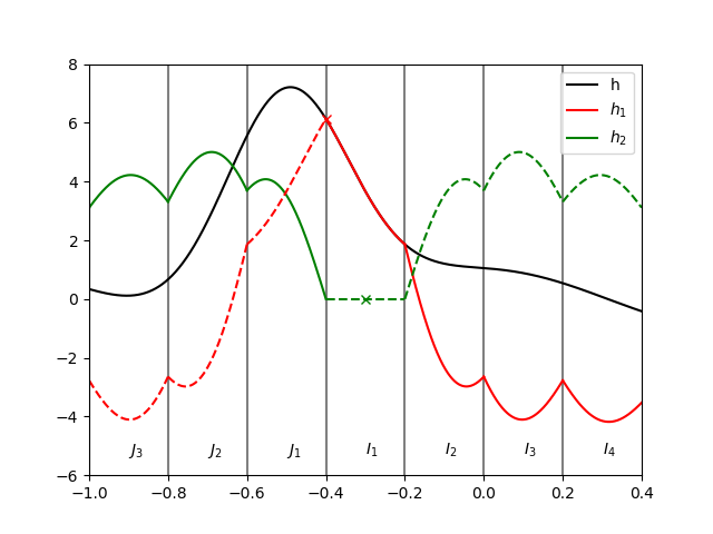
Figure 10: Visualization of the decomposition of a function $h:\mathbb{R}\rightarrow\mathbb{R}$ (black) into two symmetric functions $h_{1}$ (red) and $h_{2}$ (green), such that it holds $h=h_{1}+h_{2}$.

∎

Proof of Theorem 8.

The proof is split into several steps:

1. Based on a single center, we can approximate any given function that is symmetric with respect to that center on a finite interval:
   Let $\varphi$ be a radial basis function as specified in Assumption 2. As we only consider a single center for now, say $z_{1}$, we have

   $$F_{2}^{(j)}(x)=(f_{2}\circ f_{1})(x)^{(j)}=\sum_{i=1}^{1}\alpha_{2,i}^{(i)}\varphi(|(A(x-z_{i}))^{(j)}|),~{}1\leq j\leq d_{1}=d_{2}$$

   Now we choose the rows of the matrix $A$ as positive multiples of each other, i.e. $\sigma_{j}\cdot a$, with $0\neq a\in\mathbb{R}^{d_{0}},\sigma_{j}\geq 0,i=1,..,d_{1}=d_{2}$. Then we have

   $$F_{2}^{(j)}(x) =\alpha_{2,1}^{(j)}\varphi(|\sigma_{j}a^{\top}(x-z_{1})|),~{}1\leq j\leq d_{1}=d_{2}$$

   $$=\alpha_{2,1}^{(j)}\varphi(|\sigma_{j}x_{a}|),~{}~{}x_{a}:=a^{\top}(x-z_{1})\in\mathbb{R},$$

   which is a scalar valued function in $x_{a}$. Now choose the last mapping $f_{3}$ such that a summation is realized, i.e. $A_{3}=(1,1,..,1)^{\top}$, such that

   $$s_{1}(x_{a}):=\sum_{j=1}^{d_{2}}\alpha_{2,1}^{(j)}\varphi(|\sigma_{j}x_{a}|).$$ (14)

   This expression satisfies $s_{1}(-x_{a})=s_{1}(x_{a})$, thus only consider $x_{a}\geq 0$:

   Due to Assumption 2 it holds that $\operatorname*{span}\{\varphi(\sigma x_{a}),\sigma\geq 0\}$ is dense in $C([0,2\sqrt{d}\|a\|])$. Hence for sufficiently large $d_{2}$ and suitable coefficients $\alpha_{2,1}^{(j)}$ and $\sigma_{j}\geq 0$, the sum $s_{1}(x_{a})=\sum_{j=1}^{d_{2}}\alpha_{2,1}^{(j)}\varphi(|\sigma_{j}x_{a}|),x_{a}\geq 0$ from Equation (14) approximates any function on $C([0,2\sqrt{d}\|a\|])$ to arbitrary accuracy:

   $$\forall_{\epsilon>0,f\in C([0,2\sqrt{d}\|a\|])}~{}~{}\exists_{d_{2}\in\mathbb{N},\alpha_{2,1}^{(j)},\sigma_{j}\in\mathbb{R},j=1,..,d_{2}}$$

   $$\quad\quad\forall_{x_{a}\in[0,2\sqrt{d}\|a\|]}~{}~{}\bigg{|}f(x_{a})-\underbrace{\sum_{j=1}^{d_{2}}\alpha_{2,1}^{(j)}\varphi(|\sigma_{j}x_{a}|)}_{s_{1}(x_{a})}\bigg{|}<\epsilon.$$

   For $x_{a}\in[-2\sqrt{d}\|a\|,2\sqrt{d}\|a\|]$ the function $s_{1}(x_{a})$ corresponds to a symmetric function in $C([-2\sqrt{d}\|a\|,2\sqrt{d}\|a\|])$.

2. Leveraging Lemma 19, it is possible to approximate any given function that is univariate in direction $a\in\mathbb{R}^{d_{0}}$ on a finite interval:
   First of all, according to Lemma 19, decompose $h\in C([-2\sqrt{d}\|a\|,2\sqrt{d}\|a\|])$ into $h=h_{1}+h_{2}$, whereby $h_{i}$ satisfies $h_{i}(a^{\top}z_{i}+y)=h_{i}(a^{\top}z_{i}-y)$ for $y\geq 0,i=1,2$. Here we assume for now that both symmetry centers are different, i.e. $a^{\top}z_{1}\neq a^{\top}z_{2}\Leftrightarrow a^{\top}(z_{1}-z_{2})\neq 0\Leftrightarrow a\not\perp z_{1}-z_{2}$ is required. This requirement will be addressed in the next step. We have:

   $$h(a^{\top}x) =h_{1}(a^{\top}x)+h_{2}(a^{\top}x)$$

   $$=h_{1}(a^{\top}z_{1}+a^{\top}(x-z_{1}))+h_{2}(a^{\top}z_{2}+a^{\top}(x-z_{2}))$$

   $$=:\tilde{h}_{1}(a^{\top}(x-z_{1}))+\tilde{h}_{2}(a^{\top}(x-z_{2}))$$

   Both $\tilde{h}^{(1)}$ and $\tilde{h}^{(2)}$ are symmetric in their input with respect to zero. Therefore according to the first step, there exist $s_{1},s_{2}$ such that

   $$\forall y\in[-2\sqrt{d}\|a\|,2\sqrt{d}\|a\|]\qquad|\tilde{h}_{1}(y)-s_{1}(y)|< \frac{\epsilon}{2}$$

   $$\text{and}~{}|\tilde{h}_{2}(y)-s_{2}(y)|< \frac{\epsilon}{2}.$$

   Thus it is possible to estimate:

   $$~{}|h(a^{\top}x)-s_{1}(a^{\top}(x-z_{1}))-s_{2}(a^{\top}(x-z_{2}))|$$

   $$\leq ~{}|\tilde{h}_{1}(a^{\top}(x-z_{1}))-s_{1}(a^{\top}(x-z_{1}))|+|\tilde{h}_{2}(a^{\top}(x-z_{2}))-s_{2}(a^{\top}(x-z_{2}))|$$

   $$\leq ~{}\frac{\epsilon}{2}+\frac{\epsilon}{2}=\epsilon$$

   which holds for $x\in[0,1]^{d}$, as $|a^{\top}(x-z_{i})|\leq 2\sqrt{d}\|a\|,~{}i=1,2$.

3. Finally the approximation of arbitrary univariate functions from the second step is extended to the multivariate input case. For this, a Theorem from Vostrecov and Kreines is used [28, Theorem 3.2]:

   Theorem 20 (Special case of Vostrecov and Kreines, 1961).

   The space $\operatorname*{span}\{g(a^{\top}x)~{}|~{}g\in C(\mathbb{R}),a\in\mathcal{A}\}$ for a given $\mathcal{A}\subset\mathbb{R}^{d}$ is dense in $C(\mathbb{R}^{d})$, if $\mathcal{A}$ contains a (relatively) open subset of the unit sphere $\mathbb{S}^{d-1}\equiv\{y~{}|~{}\|y\|=1\}$.

   We pick $\mathcal{A}:=\{y\in\mathbb{S}^{d-1}~{}|~{}\|y-\frac{z_{1}-z_{2}}{\|z_{1}-z_{2}\|}\|<\frac{1}{2}\}\subset\mathbb{S}^{d-1}$ which is a relatively open subset. This choice of $\mathcal{A}$ yields

   $$\frac{1}{4}>\left\lVert y-\frac{z_{1}-z_{2}}{\|z_{1}-z_{2}\|}\right\rVert^{2} =\|y\|^{2}+\left\lVert\frac{z_{1}-z_{2}}{\|z_{1}-z_{2}\|}\right\rVert^{2}-2\left\langle y,\frac{z_{1}-z_{2}}{\|z_{1}-z_{2}\|}\right\rangle$$

   $$\Leftrightarrow~{}~{}\left\langle y,\frac{z_{1}-z_{2}}{\|z_{1}-z_{2}\|}\right\rangle >1-\frac{1}{8}=\frac{7}{8}>0,$$

   i.e. $a^{\top}z_{1}\neq a^{\top}z_{2}$ for any $a\in\mathcal{A}$. Thus, the requirement $a^{\top}z_{1}\neq a^{\top}z_{2}$ of the last step is satisfied.
   Consider $f\in C([0,1]^{d})$ arbitrary. For any $\epsilon>0$, Theorem 20 gives the existence of $N\in\mathbb{N},a_{i}\in\mathcal{A},g_{i}\in C(\mathbb{R}),i=1,..,N$ such that

   $$\left|f(x)-\sum_{i=1}^{N}\alpha_{i}g_{i}(a_{i}^{\top}x)\right|<\frac{\epsilon}{2}.$$

   Step $2$ of the proof guarantees arbitrarily accurate approximation of those $\alpha_{i}g_{i}(a_{i}^{\top}x)$ for $x\in[0,1]^{d}$, i.e. $|a_{i}^{\top}x|\leq 2\sqrt{d}\|a_{i}\|$. This is possible, as $a_{i}^{\top}z_{1}\neq a_{i}^{\top}z_{2}$, which is ensured by the choice of $\mathcal{A}$. This concludes the proof.

The realization of the linear combinations is possible based on 3. ∎

References

- [1] Z. Allen-Zhu, Y. Li, and Y. Liang. Learning and generalization in overparameterized neural networks, going beyond two layers. In H. Wallach, H. Larochelle, A. Beygelzimer, F. d’Alché Buc, E. Fox, and R. Garnett, editors, Advances in Neural Information Processing Systems, volume 32. Curran Associates, Inc., 2019.
- [2] B. Bohn, C. Rieger, and M. Griebel. A representer theorem for deep kernel learning. Journal of Machine Learning Research, 20:1–32, 2019.
- [3] Y. Cho and L. K. Saul. Kernel methods for deep learning. In Y. Bengio, D. Schuurmans, J. D. Lafferty, C. K. I. Williams, and A. Culotta, editors, Advances in Neural Information Processing Systems 22, pages 342–350. Curran Associates, Inc., 2009.
- [4] A. Damianou and N. D. Lawrence. Deep Gaussian processes. In C. M. Carvalho and P. Ravikumar, editors, Proceedings of the Sixteenth International Conference on Artificial Intelligence and Statistics, volume 31 of Proceedings of Machine Learning Research, pages 207–215, Scottsdale, Arizona, USA, 2013. PMLR.
- [5] B. Diederichs and A. Iske. Improved estimates for condition numbers of radial basis function interpolation matrices. Journal of Approximation Theory, 238:38–51, 2019.
- [6] T. Driscoll and B. Fornberg. Interpolation in the limit of increasingly flat radial basis functions. Computers & Mathematics with Applications, 43(3):413–422, 2002.
- [7] D. Elbrächter, D. Perekrestenko, P. Grohs, and H. Bölcskei. Deep neural network approximation theory. arXiv preprint arXiv:1901.02220, 2020.
- [8] R. Eldan and O. Shamir. The power of depth for feedforward neural networks. In V. Feldman, A. Rakhlin, and O. Shamir, editors, 29th Annual Conference on Learning Theory, volume 49 of Proceedings of Machine Learning Research, pages 907–940, Columbia University, New York, New York, USA, 2016. PMLR.
- [9] G. E. Fasshauer and M. McCourt. Kernel-Based Approximation Methods Using MATLAB. World Scientific Publishing Co. Pte. Ltd., Hackensack, NJ, 2015.
- [10] F. Girosi and T. Poggio. Representation properties of networks: Kolmogorov’s theorem is irrelevant. Neural Computation, 1(4):465–469, 1989.
- [11] I. Goodfellow, Y. Bengio, and A. Courville. Deep Learning. MIT Press, 2016. http://www.deeplearningbook.org.
- [12] I. Gühring, M. Raslan, and G. Kutyniok. Expressivity of deep neural networks. arXiv preprint arXiv:2007.04759, 2020.
- [13] B. Hanin. Universal function approximation by deep neural nets with bounded width and ReLU activations. Mathematics, 7(10), 2019.
- [14] K. Hornik, M. Stinchcombe, and H. White. Multilayer feedforward networks are universal approximators. Neural Networks, 2(5):359–366, 1989.
- [15] A. Jacot, F. Gabriel, and C. Hongler. Neural tangent kernel: Convergence and generalization in neural networks. arXiv preprint arXiv:1806.07572, 2018.
- [16] G. S. Kimeldorf and G. Wahba. A correspondence between Bayesian estimation on stochastic processes and smoothing by splines. The Annals of Mathematical Statistics, 41(2):495–502, 04 1970.
- [17] E. Larsson and B. Fornberg. Theoretical and computational aspects of multivariate interpolation with increasingly flat radial basis functions. Computers & Mathematics with Applications, 49(1):103–130, 2005.
- [18] L. Le, J. Hao, Y. Xie, and J. Priestley. Deep kernel: Learning kernel function from data using deep neural network. In 2016 IEEE/ACM 3rd International Conference on Big Data Computing Applications and Technologies (BDCAT), pages 1–7, 2016.
- [19] M. Leshno, V. Y. Lin, A. Pinkus, and S. Schocken. Multilayer feedforward networks with a nonpolynomial activation function can approximate any function. Neural Networks, 6(6):861–867, 1993.
- [20] G. Lorentz, M. von Golitschek, and Y. Makovoz. Constructive approximation: advanced problems. Grundlehren der mathematischen Wissenschaften. Springer, 1996.
- [21] S. Ma and M. Belkin. Diving into the shallows: A computational perspective on large-scale shallow learning. In Proceedings of the 31st International Conference on Neural Information Processing Systems, NIPS’17, page 3781–3790, Red Hook, NY, USA, 2017. Curran Associates Inc.
- [22] S. Ma and M. Belkin. Kernel machines that adapt to GPUs for effective large batch training. In Conference on Systems and Machine Learning (SysML), 2019.
- [23] G. Meanti, L. Carratino, L. Rosasco, and A. Rudi. Kernel methods through the roof: Handling billions of points efficiently. In H. Larochelle, M. Ranzato, R. Hadsell, M. F. Balcan, and H. Lin, editors, Advances in Neural Information Processing Systems, volume 33, pages 14410–14422. Curran Associates, Inc., 2020.
- [24] C. A. Micchelli, Y. Xu, and H. Zhang. Universal kernels. Journal of Machine Learning Research, 7:2651–2667, June 2006.
- [25] S. Müller and R. Schaback. A Newton basis for kernel spaces. Journal of Approximation Theory, 161(2):645–655, 2009.
- [26] H. Owhadi and G. R. Yoo. Kernel flows: From learning kernels from data into the abyss. Journal of Computational Physics, 389:22–47, 2019.
- [27] A. Paszke, S. Gross, F. Massa, A. Lerer, J. Bradbury, G. Chanan, T. Killeen, Z. Lin, N. Gimelshein, L. Antiga, A. Desmaison, A. Kopf, E. Yang, Z. DeVito, M. Raison, A. Tejani, S. Chilamkurthy, B. Steiner, L. Fang, J. Bai, and S. Chintala. Pytorch: An imperative style, high-performance deep learning library. In Advances in Neural Information Processing Systems 32, pages 8024–8035. Curran Associates, Inc., 2019.
- [28] A. Pinkus. Approximation theory of the MLP model in neural networks. Acta numerica, 8(1):143–195, 1999.
- [29] A. Rahimi and B. Recht. Random features for large-scale kernel machines. In Advances in Neural Information Processing Systems 20. MIT Press, 2008.
- [30] G. Santin and B. Haasdonk. Kernel methods for surrogate modeling. ArXiv 1907.10556, 2019.
- [31] S. Scardapane, S. Van Vaerenbergh, S. Totaro, and A. Uncini. Kafnets: Kernel-based non-parametric activation functions for neural networks. Neural Networks, 110:19–32, 2019.
- [32] B. Schölkopf, R. Herbrich, and A. J. Smola. A generalized representer theorem. In D. Helmbold and B. Williamson, editors, Computational Learning Theory, pages 416–426, Berlin, Heidelberg, 2001. Springer Berlin Heidelberg.
- [33] I. Steinwart, P. Thomann, and N. Schmid. Learning with hierarchical Gaussian kernels. arXiv preprint arXiv:1612.00824, 2016.
- [34] M. Telgarsky. benefits of depth in neural networks. In V. Feldman, A. Rakhlin, and O. Shamir, editors, 29th Annual Conference on Learning Theory, volume 49 of Proceedings of Machine Learning Research, pages 1517–1539, Columbia University, New York, New York, USA, 23–26 Jun 2016.
- [35] M. Unser. A representer theorem for deep neural networks. Journal of Machine Learning Research, 20(110):1–30, 2019.
- [36] H. Wendland. Scattered Data Approximation, volume 17. Cambridge University Press, 2005.
- [37] T. Wenzel, M. Kurz, A. Beck, G. Santin, and B. Haasdonk. Structured deep kernel networks for data-driven closure terms of turbulent flows. arXiv preprint arXiv:2103.13655, 2021. Submitted to 13th International Conference on Large-Scale Scientific Computations (LSSC 2021).
- [38] C. Williams and M. Seeger. Using the Nyström method to speed up kernel machines. In T. Leen, T. Dietterich, and V. Tresp, editors, Advances in Neural Information Processing Systems, volume 13, pages 682–688. MIT Press, 2001.
- [39] A. G. Wilson, Z. Hu, R. Salakhutdinov, and E. P. Xing. Deep kernel learning. In A. Gretton and C. C. Robert, editors, Proceedings of the 19th International Conference on Artificial Intelligence and Statistics, volume 51, pages 370–378, 2016.
- [40] H. Xue, Z.-F. Wu, and W.-X. Sun. Deep spectral kernel learning. In Proceedings of the Twenty-Eighth International Joint Conference on Artificial Intelligence, IJCAI-19, pages 4019–4025. International Joint Conferences on Artificial Intelligence Organization, 7 2019.
- [41] D. Yarotsky. Error bounds for approximations with deep ReLU networks. Neural Networks, 94:103–114, 2017.